1

Solving the MHD Equations by the Space-Time

Conservation Element and Solution Element Method

Moujin Zhang1, S.-T. John Yu1*, S.-C. Henry Lin2, Sin-Chung Chang3, and Isaiah Blankson

1Mechanical Engineering Department, the Ohio State University, Columbus, OH 43202 2General Motor Corporation, Warren, MI 48090 3NASA Glenn Research Center, Cleveland, OH 44135

Keywords: MHD, the CESE method, constraint transport

*Corresponding Author: Professor S.-T. John Yu Mechanical Engineering Department The Ohio State University 650 Ackerman Road, Suite #255 Columbus, OH 43202 Tel: 614-292-2902 Fax: 614-292-3163

2

Abstract

We apply the Space-Time Conservation Element and Solution Element (CESE) method

to solve the ideal MHD equations with special emphasis on satisfying the divergence free

constraint of magnetic field, i.e., ∇⋅B = 0. In the setting of the CESE method, four

approaches are employed: (i) the original CESE method without any additional treatment,

(ii) a simple corrector procedure to update the spatial derivatives of magnetic field B after

each time marching step to enforce ∇⋅B = 0 at all mesh nodes, (iii) an constraint-transport

method by using a special staggered mesh to calculate magnetic field B, and (iv) the

projection method by solving a Poisson solver after each time marching step. To

demonstrate the capabilities of these methods, two benchmark MHD flows are calculated

(i) a rotated one-dimensional MHD shock tube problem, and (ii) a MHD vortex problem.

The results show no differences between different approaches and all results compare

favorably with previously reported data.

3

1 Introduction

While many Computational Fluid Dynamics (CFD) methods have been successfully

developed for gas dynamics, extension of these methods for solving the Magneto-Hydro-

Dynamic (MHD) equations involves unique requirements and poses greater challenges

[1-14]. In particular, for multi-dimensional MHD problems, it is critical to maintain the

divergence-free constraint of magnetic field, i.e., ∇⋅B = 0, at all locations in the space-

time domain. Analytically, the constraint is ensured if it is satisfied in the initial condition.

However, it has been difficult to maintain this constraint in calculating evolving MHD

problems. Violating the constraint allows numerical errors to be accumulated over the

computational time, leading to erroneous solutions and/or numerical instability.

To satisfy ∇⋅B = 0, a special treatment directly incorporated into the CFD method

employed is often required. Special treatments have been categorized into three groups: (i)

The projection method, e.g., Brackbill and Barnes [5]: At each time step, the method

solves a Poisson equation to update the magnetic field to enforce ∇⋅B = 0. (ii) The eight-

wave formulation by Powell [6]: ∇⋅B is not treated as zero in deriving the MHD

equations, leading to additional source/sink terms in equations for B. The CFD solver

employed would activate the sink/source terms to counter the unbalanced ∇⋅B in

numerical solutions. (iii) The constrained-transport procedure, e.g., Evans and Hawley

[7], Dai and Woodward [8], Balsara and Spice [9], and Toth [12], based on the use of

staggered mesh to enforce the constraint at certain spots of the control volume. Various

versions of these three approaches have been developed to solve the MHD equations in

multiple spatial dimensions [4-13]. Recently, these methods have been assessed and

summarized by Toth [12].

4

In the present paper, we report the application of the Space-Time Conservation

Element and Solution Element (CESE) method [17-20] to solve the two-dimensional

MHD equations. Four approaches are employed: (i) the original CESE method without

any additional treatment for ∇⋅B = 0, (ii) a simple modification procedure to update the

spatial derivatives of B after each time marching step such that ∇⋅B = 0 is enforced at all

mesh nodes, (iii) an extended CESE method based on the constraint-transport procedure,

and (iv) the projection method coupled with the CESE method. The approach (i) is trivial.

Nevertheless, its results are comparable with other results by the three other approaches.

Approaches (ii) and (iii) are new schemes for ∇⋅B = 0. Approach (iv), the projection

method, is a conventional and reliable approach to impose ∇⋅B = 0. All results in the

present paper compare well with previously published data.

The rest of the paper is arranged as follows. Section 2 illustrates the governing

equations. Section 3 provides a brief review of the CESE method for two-spatial-

dimensional problems. Section 4 shows the new CESE schemes, i.e., approaches (ii) and

(iii), for ∇⋅B = 0. Section 5 provides the results and discussions. We then offer

conclusions and provide cited references.

2 Governing Equations

The ideal MHD equations include the continuity, the momentum, the energy, and the

magnetic induction equations. In two spatial dimensions, the dimensionless equations can

be cast into the following conservative form:

0=∂∂

+∂∂

+∂∂

yxtGFU

, (2.1)

5

where

( ) ( )TTzyx uuuuuuuuBBBewvu 87654321 ,,,,,,,,,,,,,, == ρρρρU , (2.2)

( ) ( ) ( )

=

−−

++−+−−

−+

=

8

7

6

5

4

3

2

1

0

20

2

0

ffffffff

wBuBvBuB

wBvBuBBupeBBuwBBuvBpu

u

xz

xy

zyxx

zx

yx

x

ρρ

ρρ

UF , (2.3)

and

( ) ( ) ( )

=

−

−++−+

−−+

−

=

8

7

6

5

4

3

2

1

0

20

2

0

gggggggg

wBvB

uBvBwBvBuBBvpe

BBvwBpv

BBvuv

yz

yx

zyxy

zy

y

xy

ρρρ

ρ

UG . (2.4)

In the above equations, ρ, p and e are density, pressure and specific total energy,

respectively; u, v, and w are velocity components and Bx, By and Bz are magnetic field

components in the x, y, and z directions, respectively. The total pressure and the specific

total energy are

( ) 22220 zyx BBBpp +++= , (2.5)

( ) ( ) 22 222222zyx BBBwvue ++++++= ρρε . (2.6)

6

For calorically ideal gases, the specific internal energy ε can be expressed as

( ) ( )11 −=

−=

γργε

RTp, (2.7)

where γ is the specific heat ratio, T is temperature, and R is the gas constant. To proceed,

we apply the chain rule to Eq. (2.1) and obtain

0=∂∂

+∂∂

+∂∂

yxty U

JU

JU x , (2.8)

where Jx and Jy are Jacobian matrices of the spatial fluxes in the x and y directions,

respectively. The components of the matrices are listed in Appendix. The eigenvalues of

matrix Jx are xfcu ± , x

acu ± , xscu ± , u and u, where x

ac , xsc and x

fc are the speeds of the

Alfvan wave, the slow shock wave, and the fast shock wave, respectively, and they are

defined as

ρxxa Bc = , (2.9)

21222

22 421

−

⋅++

⋅+=

ρρρxx

f

Bcccc

BBBB , (2.10)

21222

22 421

−

⋅+−

⋅+=

ρρρxx

s

Bcccc

BBBB . (2.11)

In Eqs. (2.10-11), ργpc = is the speed of sound. Similarly, the eigenvalues of matrix

yJ are yfcv ± , y

acv ± , yscv ± , v and v, where y

ac , ysc and y

fc are defined as

ρyy

a Bc = , (2.12)

7

21222

22 421

−

⋅++

⋅+=

ρρρyy

f

Bcccc

BBBB , (2.13)

21222

22 421

−

⋅+−

⋅+=

ρρρyy

s

Bcccc

BBBB . (2.14)

3 The CESE Method

The above MHD equations can be expressed as

0=∂

∂+

∂∂

+∂

∂y

gxf

tu mmm , m = 1, 2, … , 8, (3.1)

where mu , mf and mg are the entries of the flow variable vector and the flux vectors in

the x and y directions, respectively, and m is the index for the equation. Let

xx =1 , yx =2 and tx =3 be the coordinates of a three-dimensional Euclidean space

3E , Eq. (3.1) becomes a divergence free condition:

0=⋅∇ mh , m = 1, 2, … , 8, (3.2)

where ( )mmmm ugf ,,=h are the current density vector. By using Gauss’ divergence

theorem in 3E , we have

( )0=⋅=⋅∇ ∫∫ VS m

Vm ddV shh , m = 1, 2, … , 8, (3.3)

where (i) S(V) is the boundary of an arbitrary space-time region V in 3E , and (ii)

σdd ns = with σd and n, respectively, are the area and the unit outward normal of a

8

surface element on S(V). The CESE method integrates Eq. (3.3) for the evolving flow

variables.

For completeness, we will briefly illustrate the CESE method based on the

following three parts: (i) The definition of SE and CE in the space-time domain. (ii) The

integration of Eq. (3.3) over a CE to form the algebraic equations for the flow variables at

a new time step. (iii) The re-weighting procedure with added artificial damping in

calculating the gradients of the flow variables. The discussion of the CESE method here

will be based on the modified CESE method for a quadrilateral mesh [19]. To be concise,

our discussion of the CESE method will be focused on a uniform quadrilateral mesh.

3.1 Definition of Solution Element and Conservation Element

In Fig. 1, the spatial domain is divided into non-overlapping quadrilaterals and any two

neighboring quadrilaterals share a common side. The centroid of each quadrilateral is

marked by either a hollow circle or a solid circle. Point G, the centroid of quadrilateral

ABCD, is marked by a solid circle, while the points N, E, W and S are the centroids of the

four neighboring quadrilaterals, and are marked by hollow circles. Because of the

uniform mesh, G is also the centroid of polygon NAWBSCED, which coincides with

quadrilateral NWSE. Let j, k and n be the indices for x, y, and t, respectively. Shown in

Fig. 2, points A, B, C, D, N, E, W, S and G are at the time level n-1/2; points A’, B’, C’,

D’, N’, E’, W’, S’ and G’ are at the time level n; and points A”, B”, C”, D”, N”, E”, W”,

S” and G” are at the time level n+1/2.

As shown in Fig. 2, the solution element SE(j, k, n) associated with point G’ is

defined as the union of three quadrilateral planes, N’W’S’E’, A”ACC”, B”BDD”, and

9

their immediate neighborhoods. Its spatial projection is shown in Fig. 1 as the dashed

lines. Similarly, associated with points N, E, W, and S, there are four solution elements:

SE(j, k+1/2, n-1/2), SE (j+1/2, k, n-1/2), SE (j-1/2, k, n-1/2), and SE (j, k-1/2, n-1/2). To

calculate the unknowns at G’, the algebraic equations are derived based on space-time

flux conservation involved flow solutions at points G’, N, E, W, and S, referred to as the

solution points. Point G’, located at t = tn is staggered with respect to points N, E, W, and

S at t = tn-1/2.

As shown in Fig. 2, a space-time cylinder can be formed with surfaces associated

with SE(j, k, n) and surfaces associated with one of the four SEs at the time level n-1/2.

For instance, cylinder N’A’G’D’NAGD is formed by surfaces associated with SE(j, k, n)

and SE(j, k+1/2, n-1/2) . This cylinder is one of the Basic Conservation Elements (BCE)

of point G’. There are three other BCEs associated with point G’, i.e., A’W’B’G’AWBG,

B’S’C’G’BSCG and C’E’D’G’CEDG. The union of these four BCEs forms a

Compounded Conservation Element (CCE) N’W’S’E’NWSE with its top center at point

G’.

3.2 The Space-Time Integration

Inside SE(j, k, n), the discretized variables and fluxes, denoted with a superscript *, are

assumed to be linear. For m = 1, 2, … , 8, let

( ) ( ) ( ) ( ) ( ) ( ) ( ) ( )nnkjmtkj

n

kjmykjn

kjmxn

kjmm ttuyyuxxuunkjtyxu −+−+−+= ,,,,,,* ,,;,, ,

(3.4)

( ) ( ) ( ) ( ) ( ) ( ) ( ) ( )nnkjmtkj

n

kjmykjn

kjmxn

kjmm ttfyyfxxffnkjtyxf −+−+−+= ,,,,,,* ,,;,, ,

(3.5)

10

( ) ( ) ( ) ( ) ( ) ( ) ( ) ( )nnkjmtkj

n

kjmykjn

kjmxn

kjmm ttgyygxxggnkjtyxg −+−+−+= ,,,,,,* ,,;,, ,

(3.6)

where ( )nkjmu , , ( )n

kjmf , , ( )nkjmg , , ( )n

kjmxu , , ( )n

kjmyu,

, ( )nkjmtu , , ( )n

kjmxf , , ( )n

kjmyf,

, ( )nkjmtf , ,

( )nkjmxg , , ( )n

kjmyg,

,and ( )nkjmtg , are flow variables, fluxes, and their first-order derivatives at

point G’. Aided by the chain rule we have

( ) ( ) ( )∑=

=8

1,,,,

l

nkjlx

n

kjlmn

kjmx uff , m = 1, 2, … , 8, (3.7)

( ) ( ) ( )∑=

=8

1,,,,

l

nkjlx

n

kjlmn

kjmx ugg , m = 1, 2, … , 8 (3.8)

( ) ( ) ( )∑=

=8

1,,,,

l

n

kjlyn

kjlmn

kjmy uff , m = 1, 2, … , 8 (3.9)

( ) ( ) ( )∑=

=8

1,,,,

l

n

kjlyn

kjlmn

kjmy ugg , m = 1, 2, … , 8 (3.10)

where ( )n

kjlmf,, , ( )n

kjlmg,, are the (m, l)th entries of the Jacobian matrixes Jx and Jy in the x

and y directions, respectively. To proceed, we assume that ( )nkjtyxum ,,;,,* ,

( )nkjtyxfm ,,;,,* and ( )nkjtyxgm ,,;,,* satisfy the original MHD equations, Eq. (3.1), at

point, (j, k, n):

( ) ( ) ( )n

kjmyn

kjmxn

kjmt gfu,,, −−= , m = 1, 2, … , 8. (3.11)

Aided by Eqs. (3.7) and (3.10), , Eq. (3.11) becomes

( ) ( ) ( ) ( ) ( )∑∑==

−−=8

1,,,

8

1,,,,

l

n

kjlyn

kjlml

nkjlx

n

kjlmn

kjmt ugufu , m = 1, 2, … , 8, (3.12)

11

Similarly, for m = 1, 2, … , 8, we have

( ) ( ) ( )∑=

=8

1,,,,

l

nkjlt

n

kjlmn

kjmt uff ( ) ( ) ( ) ( ) ( )[ ]∑ ∑= =

+−=8

1

8

1,,,,,,,,

l r

n

kjryn

kjrln

kjrxn

kjrln

kjlm uguff ,

(3.13)

( ) ( ) ( )∑=

=8

1,,,,

l

nkjlt

n

kjlmn

kjmt ugg ( ) ( ) ( ) ( ) ( )[ ]∑ ∑= =

+−=8

1

8

1,,,,,,,,

l r

n

kjryn

kjrln

kjrxn

kjrln

kjlm ugufg .

(3.14)

Therefore, a set of given values of ( )nkjmu , , ( )n

kjmxu , and ( )n

kjmyu,

completely determine the

distribution of the flow variables and fluxes, i.e., Eqs., (3.4-6), inside SE(j, k, n). Thus the

flow variables ( )nkjmu , and their spatial gradients ( )n

kjmxu , and ( )n

kjmyu,

are the unknowns to

be solved in the CESE method.

The time marching scheme to calculate ( )nkjmu , is based on integrating Eq. (3.3)

over the CCE associated with point G’. Recall that the CCE is a quadrilateral cylinder

with surfaces associated with five different SEs. The top surface, quadrilateral N’W’S’E’

belongs to SE(j, k, n); quadrilaterals NAGD, N’A’AN and N’D’DN belong to SE(j, k+1/2,

n-1/2); quadrilaterals WAGB, W’A’AW and W’B’BW belong to SE(j-1/2, k, n-1/2);

quadrilaterals SBGC, S’B’BS and S’C’CS belong to SE(j, k-1/2, n-1/2); and quadrilaterals

EDGC, E’C’CE and E’D’DE belong to SE(j+1/2, k, n-1/2).

The flux leaving each planar surface of the CCE is equal to the inner product of the

current density vector ( )**** ,, mmmm ugf=h , evaluated at the centroid of the surface, and the

surface vector s = nS. For example, the top surface of the CCE is quadrilateral N’W’S’E’

with an area Stop and the centroid is G’ (xj,k, yj,k, tn). At the centroid of the top surface of

12

the CCE, the current density vector ( ) ( ) ( )( )n

kjm

n

kjm

n

kjmm ugf ,,,* ,,=h , and the surface vector

is (0, 0, Stop). Thus the flux leaving the top surface of the CCE is

(FLUXm)top = ( )nkjmu , Stop, m = 1, 2, … , 8. (3.15)

Similarly calculation for fluxes through other surfaces of the CCE can be performed. For

surfaces associated with SE(j, k+1/2, n-1/2), the centriods of surfaces NAGD, NDD’N’

and NAA’N’ are denoted as ( )2/100 ,, −nNN tyx , ( )4/111 ,, −n

NN tyx and ( )4/122 ,, −nNN tyx ,

respectively. Their surface vectors are (0, 0, -S1), ( )0,, 11 yN

xN λλ , and ( )0,, 22 y

Nx

N λλ , where S1 is

the area of quadrilateral NAGD, and

( ) 21 tyy DNx

N ∆−=λ , (3.16)

( ) 21 txx NDy

N ∆−=λ , (3.17)

( ) 22 tyy NAx

N ∆−=λ , (3.18)

( ) 22 txx ANy

N ∆−=λ . (3.19)

The flux leaving each of the three surfaces can be calculated as the inner product of the

corresponding flux vector and the surface vector at the surface centroid. By summing up

the fluxes, for m = 1, 2, … , 8, we have,

( ) ( )( ) ( )( ) ( )2/14/122*1

12/14/122*2

2/14/111*12/14/111*1

2/12/100*1

,21,;,,,21,;,,

,21,;,,,21,;,,

,21,;,,

−−−−

−−−−

−−

++++

++++

+−=

nnNNm

ynnNNm

xN

nnNNm

yN

nnNNm

xN

nnNNmNm

tkjtyxgtkjtyxf

tkjtyxgtkjtyxf

tkjtyxuSFLUX

λλ

λλ

(3.20)

Because the solution at the time step n-1/2 is known, the value of this flux can be readily

calculated. Similarly, the fluxes leaving surfaces associated with SE(j-1/2, k, n-1/2), SE(j,

13

k-1/2, n-1/2), and SE(j+1/2, k, n-1/2) can be readily calculated. For conciseness, we

simply name these fluxes as ( )WmFLUX , ( )SmFLUX and ( )EmFLUX . As a result, the

space-time flux conservation over the CCE is

( ) ( )∑ =+NEWS

llmtopm FLUXFLUX 0 , m = 1, 2, … , 8. (3.21)

Note that only the first term in the above equation contains the unknowns to be solved at

point G’. Aided by Eq. (3.15), the flow variables at the current time step n can be

calculated by

( )( )

top

NEWS

llm

nkjm S

FLUXu

∑−=, , m = 1, 2, … , 8. (3.22)

3.3 Solutions of Flow Variable Gradients

To proceed, we calculate the spatial gradients of the flow variables ( ) ,

nmx j k

u and ( ),

n

my j ku .

The calculation is divided into two steps: (i) Finite-differencing the flow variables um at

point G’, N’, E’, W’, and S’, at t = tn to obtain four sets of mxu and myu . (ii) Apply a

reweighing procedure to the above four sets of mxu and myu to determine ( ) ,

nmx j k

u and

( ),

n

my j ku at G’. In what follows, these two calculation steps are illustrated.

Flow variables mu at point G’ are obtained from Eq. (3.22). The flow variables mu

at four neighbor points N’, W’, S’ and E’ are obtained by using the Taylor series

expansion along the time axis from the time level n-1/2, i.e., for m = 1, 2, … , 8,

14

( ) ( ) ( )1/2 1 /2'

2n n

m m mtl ll

tu u u− −∆

= + , (3.23)

where l =1, 2, 3, and 4 denoting point N’, E’, W’ and S’, respectively.

The square plane N’E’S’W’ is divided into four triangles; N’W’G’, W’S’G’, S’E’G’,

and E’N’G’. In each triangle, we finite-difference mu at the three vertices to obtain the

flow variable gradient ( ) ,

nmx j k

u and ( ),

n

my j ku . Consider triangle ∆N’W’G’, the flow variable

gradient at its centroid can be expressed as,

( )( ) ∆∆= xGmxu '1 , (3.24)

( )( ) ∆∆= yGmyu'

1 , (3.25)

where

( ) ( )( ) ( ) GWGmWm

GNGmNmx

yyuu

yyuu

−−

−−=∆

'''

'''

, (3.26)

( ) ( )( ) ( ) WGGmWm

NGGmNmy

xxuu

xxuu

−−

−−=∆

'''

'''

, (3.27)

GWGW

GNGN

yyxxyyxx

−−−−

=∆ , (3.28)

and

( ) ( )nkjmGm uu ,' = . (3.29)

15

For triangles ∆W’S’G’, ∆S’E’G’ and ∆E’N’G’, the flow variable gradients at their

centroids, denoted by ( )( ) '2

Gmxu , ( )( )'

2Gmyu , ( )( ) '

3Gmxu , ( )( )

'3

Gmyu , ( )( ) '4

Gmxu and ( )( )'

4Gmyu , can be

obtained in a similar way.

To proceed, a re-weighting procedure is applied to the four sets of flow variable

gradients to obtain the final flow variable gradient at G’, i.e., for m = 1, 2, … , 8,

( ) ( ) ( )( )[ ] ( )∑∑ ===

4

1

4

1 ', ll

ml Gl

mxl

m

n

kjmx WuWuαα , (3.30)

( ) ( ) ( )( )[ ] ( )∑∑ ===

4

1

4

1 ', ll

ml Gl

myl

m

n

kjmy WuWuαα

, (3.31)

where

∏ ≠==

4

,1 lqq

qm

lm WW , for l =1, 2, 3, 4, (3.32)

and

( )( )[ ] ( )( )[ ]2

'

2

' Gq

myGq

mxq

m uuW += . (3.33)

For shock capturing, α = 1, or 2, is a prescribed constant. For flows without shock, we let

α = 0. As such, Eqs. (3.30-31) reduce to the standard central-differencing method.

4 Extended CESE Schemes for ∇⋅B = 0

In this section, we illustrate two new CESE schemes for ∇⋅B = 0: Schemes I and

Schemes II. Both schemes are built based on special features of the original CESE

method. Scheme I takes advantage of the fact that the flow variable gradients ( ) ,

nmx j k

u and

16

( ),

n

my j ku are directly used as the unknowns and they march in time hand-in-hand with the

flow variables ( ) ,

nm j k

u . Scheme I is a simple adjustment to the calculation of ( ) ,

nmx j k

u and

( ),

n

my j ku such that ∇⋅B = 0 is satisfied at all mesh points after each time marching step.

Scheme II takes advantage of staggered mesh arrangement in the original CESE method.

By a simple adjustment of the mesh nodes employed in calculating the magnetic flux, we

ensure the satisfaction of ∇⋅B = 0 at all solution points. In what follows, we report these

two schemes.

4.1 Scheme I

As illustrated in the above section, the flow variables ( ) ,

nm j k

u are calculated by space-

time flux conservation i.e., Eq. (3.22), over a CCE with its top center at point (j, k, n),

while the flow variable gradients ( ) ,

nmx j k

u and ( ),

n

my j ku are calculated by a combination of

a central differencing and a reweighing procedure. In Scheme I, we first follow the above

CESE algorithm to calculate the flow variables and their spatial gradients. After each

time marching step, a corrector step is applied to adjust the values of n

kj

x

xB

,

∂∂ and

n

kj

y

yB

,

∂

∂. The calculated results of all other unknowns remain intact. Note that

n

kj

x

xB

,

∂∂ and

n

kj

y

yB

,

∂

∂are denoted as ( )n

kjxu ,5 and ( )n

kjxu ,6 in Eq. (2.2). The adjustments to

these two terms are

17

( ) ( ) ( ) ( )[ ]n

kjy

n

kjx

n

kjx

new

kjx uuuu,6,5,5,5 2

1+−= , (4.1)

( ) ( ) ( ) ( )[ ]n

kjy

n

kjx

n

kjy

new

kjy uuuu,6,5,6,6 2

1+−= , (4.2)

where the updated gradient is denoted by the superscript new. By adding the two

equations above, we yield

( ) ( ) 0,6,5 =+

new

kjynew

kjx uu . (4.3)

That is, with the additional treatment for kj

x

xB

,

∂∂ and

kj

y

yB

,

∂

∂by Eqs. (4.1-2), the

constraint ( ) 0, =⋅∇ kjB is satisfied at each mesh node in each time marching step.

4.2 Scheme II

Scheme II is based on a specially defined SE for solving the magnetic induction

equations. As illustrated in Fig. 3, the Special Conservation Element (SCE) associated

with point G’ is defined as quadrilateral P’Q’R’T’PQRT, which composes of six planes:

P’Q’R’T’, P’Q’QP, Q’R’RQ, R’T’TR, T’P’PT and PQRT. The six planes are referred to

as Special Solution Elements (SSE). The SSE and SCE are defined for solving magnetic

field components Bx and By only. Shown in Fig. 3, the solution points N’, E’, W’, and S’

surrounding G’ are at the middle of line segments P’Q’, P’T’, Q’R’ and R’T’,

respectively. Thus the SCE here includes a space-time region larger than the original

CCE.

To proceed, the SSEs, P’Q’R’T’ and PQRT, are defined to be associated with the

solution points G’ and G, respectively. Similarly, the SSEs, P’Q’QP, Q’R’RQ, R’T’TR

18

and T’P’PT are associated with the solution points N, W, S and E, respectively. Inside

SSEs, the profiles of Bx and By follow the first-order Taylor series expansion. For

example, we consider SSE P’Q’QP associated with the solution point N:

( ) ( ) ( ) ( )( ) ( ) ( ) ( )2121

21,21,21

21,

21,21

21,21

21,* 21,21,;,,

−−++

−

+

+−

+−

+

−+−+

−+=−+nn

kjmtkjn

kjmy

kjn

kjmxn

kjmm

ttuyyu

xxuunkjtyxu, (4.4)

( ) ( ) ( ) ( )( ) ( ) ( ) ( )2121

21,21,21

21,

21,21

21,21

21,* 21,21,;,,

−−++

−

+

+−

+−

+

−+−+

−+=−+nn

kjmtkjn

kjmy

kjn

kjmxn

kjmm

ttfyyf

xxffnkjtyxf, (4.5)

( ) ( ) ( ) ( )( ) ( ) ( ) ( )2121

21,21,21

21,

21,21

21,21

21,* 21,21,;,,

−−++

−

+

+−

+−

+

−+−+

−+=−+nn

kjmtkjn

kjmy

kjn

kjmxn

kjmm

ttgyyg

xxggnkjtyxg, (4.6)

where m = 6 and 7. Similar discretization procedure is employed in the other SSEs.

To proceed, we perform numerical integration of the magnetic induction

equations in x and y directions over the SCE based on the above discretization scheme for

the SSEs. The magnetic induction equations can be reformulated as

0=∂Ω∂

+∂

∂yt

Bx , (4.7)

0=∂Ω∂

−∂

∂

xt

B y , (4.8)

where Ω = vBx –uBy . Integrating Eqs. (4.7-8) over the SCE, we have

( )( )

0,,0 =⋅Ω∫ VS x dB s , (4.9)

( )( )

0,0, =⋅Ω−∫ VS y dB s . (4.10)

19

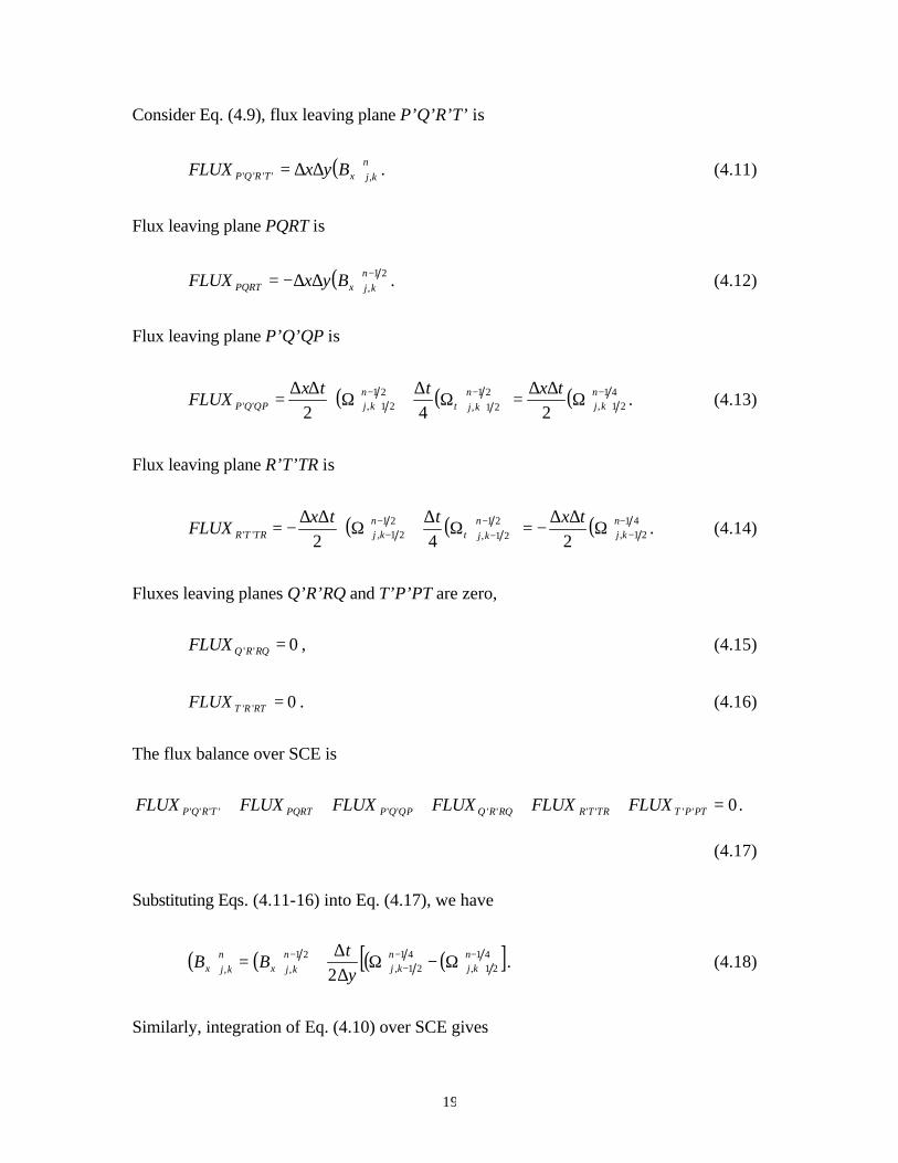
Consider Eq. (4.9), flux leaving plane P’Q’R’T’ is

( )nkjxTRQP ByxFLUX ,'''' ∆∆= . (4.11)

Flux leaving plane PQRT is

( ) 21,−∆∆−= nkjxPQRT ByxFLUX . (4.12)

Flux leaving plane P’Q’QP is

( ) ( ) ( ) 4121,

2121,

2121,'' 242

−+

−+

−+ Ω

∆∆=

Ω

∆+Ω

∆∆= n

kjn

kjtn

kjQPQP

txttxFLUX . (4.13)

Flux leaving plane R’T’TR is

( ) ( ) ( ) 4121,

2121,

2121,'' 242

−−

−−

−− Ω

∆∆−=

Ω

∆+Ω

∆∆−= n

kjn

kjtn

kjTRTR

txttxFLUX . (4.14)

Fluxes leaving planes Q’R’RQ and T’P’PT are zero,

0'' =RQRQFLUX , (4.15)

0'' =RTRTFLUX . (4.16)

The flux balance over SCE is

0'''''''''''' =+++++ PTPTTRTRRQRQQPQPPQRTTRQP FLUXFLUXFLUXFLUXFLUXFLUX .

(4.17)

Substituting Eqs. (4.11-16) into Eq. (4.17), we have

( ) ( ) ( ) ( )[ ]4121,

4121,

21,, 2

−+

−−

− Ω−Ω∆∆

+= nkj

nkj

nkjx

nkjx y

tBB . (4.18)

Similarly, integration of Eq. (4.10) over SCE gives

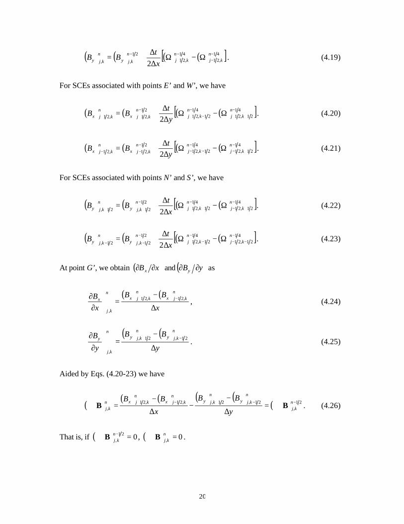
20

( ) ( ) ( ) ( )[ ]41,21

41,21

21

,, 2−−

−+

− Ω−Ω∆∆

+= nkj

nkj

n

kjyn

kjy xt

BB . (4.19)

For SCEs associated with points E’ and W’, we have

( ) ( ) ( ) ( )[ ]4121,21

4121,21

21,21,21 2

−++

−−+

−++ Ω−Ω

∆∆

+= nkj

nkj

nkjx

nkjx y

tBB . (4.20)

( ) ( ) ( ) ( )[ ]4121,21

4121,21

21,21,21 2

−+−

−−−

−−− Ω−Ω

∆∆

+= nkj

nkj

nkjx

nkjx y

tBB . (4.21)

For SCEs associated with points N’ and S’, we have

( ) ( ) ( ) ( )[ ]4121,21

4121,21

21

21,21, 2−

+−−

++−

++Ω−Ω

∆∆

+= nkj

nkj

n

kjyn

kjy xt

BB . (4.22)

( ) ( ) ( ) ( )[ ]4121,21

4121,21

21

21,21, 2−

−−−

−+−

−−Ω−Ω

∆∆

+= nkj

nkj

n

kjyn

kjy xt

BB . (4.23)

At point G’, we obtain ( )xB x ∂∂ and ( )yBy ∂∂ as

( ) ( )x

BB

xB

nkjx

nkjx

n

kj

x

∆

−=

∂∂ −+ ,21,21

,

, (4.24)

( ) ( )y

BB

y

Bn

kjyn

kjyn

kj

y

∆

−=

∂

∂ −+ 21,21,

,

. (4.25)

Aided by Eqs. (4.20-23) we have

( )( ) ( ) ( ) ( )

( ) 21,

21,21,,21,21,

−−+−+ ⋅∇=∆

−−

∆

−=⋅∇ n

kj

n

kjyn

kjyn

kjxn

kjxnkj y

BB

x

BBBB . (4.26)

That is, if ( ) 021, =⋅∇ −nkjB , ( ) 0, =⋅∇ n

kjB .

21

Based on the use of the above SSE and SCE, this extended CESE scheme is

proposed to solve Bx, By, xBx ∂∂ and yB y ∂∂ at point G’. All other variables are

calculated by using the original CESE scheme as illustrated in Section 3.

5 Results and Discussions

In this section, we report results obtained from the CESE schemes. Section 5.1 presents

the two-dimensional results of a MHD shock tube problem. Section 5.2 shows the

solution of a MHD vortex problem, which is a real two-dimensional problem. For the two

problems, we employ the new CESE schemes for maintaining ∇⋅B = 0. Moreover, for the

MHD vortex problem, we also employ the projection procedure, i.e., the Poisson solver,

for maintaining ∇⋅B = 0.

5.1 A Rotated Shock Tube Problem

In a one-dimensional problem, ∇⋅B = 0 is automatically satisfied. A common practice to

assess multi-dimensional solvers for ∇⋅B = 0 is to perform two-dimensional calculation

of an inherently one-dimensional problems formulated in the rotated coordinates such

that the one dimensionality of the flow is not aligned with the numerical mesh and ∇⋅B =

0 may not be easily satisfied. As such, the degree of deficiency in satisfying ∇⋅B = 0 can

be straightforwardly judged by direct comparison between the two-dimensional results

with the corresponding one-dimensional result. As shown in Fig. 4, the computation is

conducted in the rectangular domain OABC. The one-dimensional problem is defined

along the ξ-direction. Through coordinate rotation, flow variables in the x-y coordinates

can be transformed to be in the ξ-η coordinates, and vice versa.

22

The initial condition, defined along ξ-direction, consists of two distinct states:

( ) ( )( )

−=

rightfor 45,45,1,0,10,1leftfor 45,45,20,0,10,1

, , , , ,ππππ

ρ η zBBpvu ,

with 35=γ , w = 0, and Bz =0. The flow condition and computational parameters are

taken from Toth [12]. The computational domain is ( ) [ ] [ ]Nyx 2,01,0, ×∈ , where N is the

grid point in x direction and set to N = 256. The rotated angle is set to tan-1 2 ≈ 63.430. A

periodic condition is imposed in the η direction. The computation is up to t = 508.0 ,

and the computational domain is covered by a mesh of 256×2 grid points.

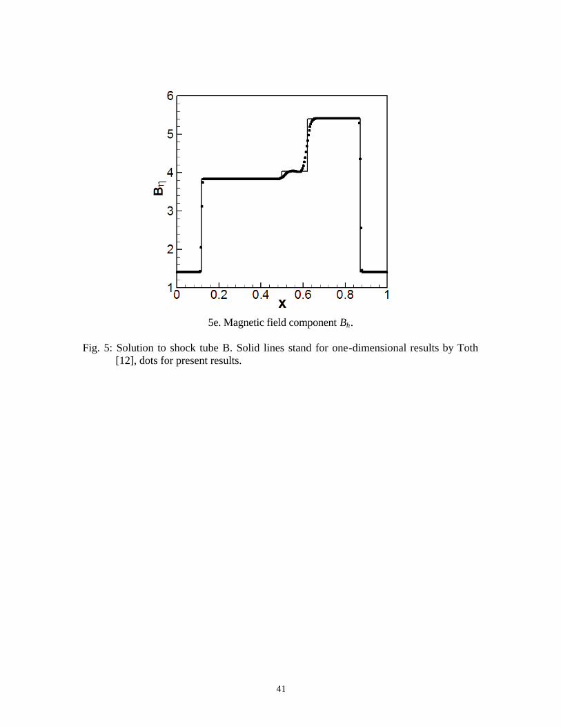
Figure 5 shows results by the original CESE scheme, in which dots denote the

present solution and solid lines represent one-dimensional solution in Toth [12]. The

right-moving waves include a fast shock, a slow shock and a contact discontinuity. The

left-moving waves include a fast shock and a slow rarefaction wave. Favorable

comparison is found between our present two-dimensional results and the one-

dimensional results. We also employed the new schemes proposed in Section 4 for this

problem. Figure 6 shows the comparison of the pressure and magnetic field component

Bη profiles obtained by using (i) the original CESE scheme, (ii) the scheme I with a

simple adjustment and (iii) the scheme II based on the constraint-transport procedure. For

shock capturing, there is no obvious difference between the original CESE scheme and

the new schemes.

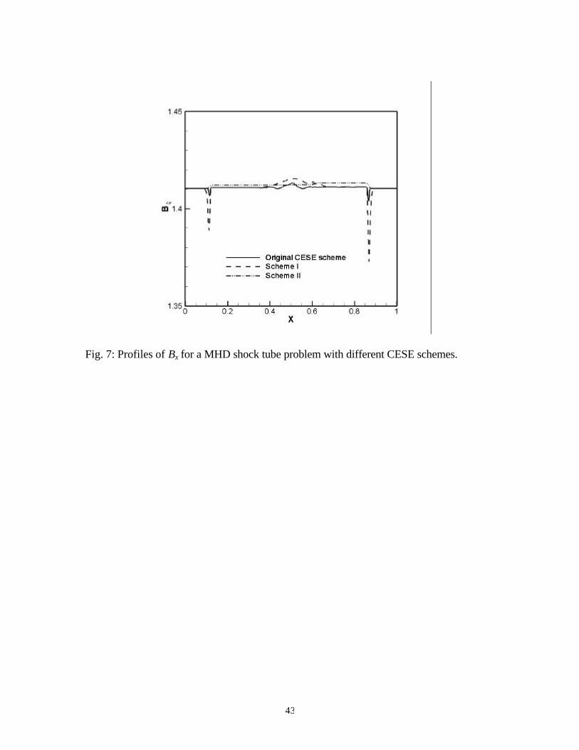
Analytically, Bξ is constant along the ξ direction. Figure 7 shows the Bξ profiles

calculated by the three different CESE schemes. We observe oscillations around the

moving shocks. The oscillations with the original scheme are smaller than that with

23

scheme I, and are comparable with that with scheme II. Away from shocks, the solutions

are smooth.

The same assessment was conducted by Toth [12] by using several special

treatments for ∇⋅B = 0, including the 8-wave method, various versions of the constraint

transport methods, and projection method. Refer to Fig. 11 in [12], oscillations of Bξ

occur around shocks for all approaches employed. Comparing with the results shown by

Toth [12], the magnitudes of Bξ oscillations near the moving shocks calculated by the

present three CESE methods are much smaller. Moreover, as shown in Fig. 14 of Toth

[12], spurious oscillations of other variable were also observed. In our case, as shown in

Fig. 6, no oscillation is observed in present results. Without using a special treatment for

∇⋅B = 0, the calculated results compare favorably with one-dimensional data. With the

use of special treatments for ∇⋅B = 0, i.e., Scheme I and II, illustrated in Section 4, no

obvious improvement is observed.

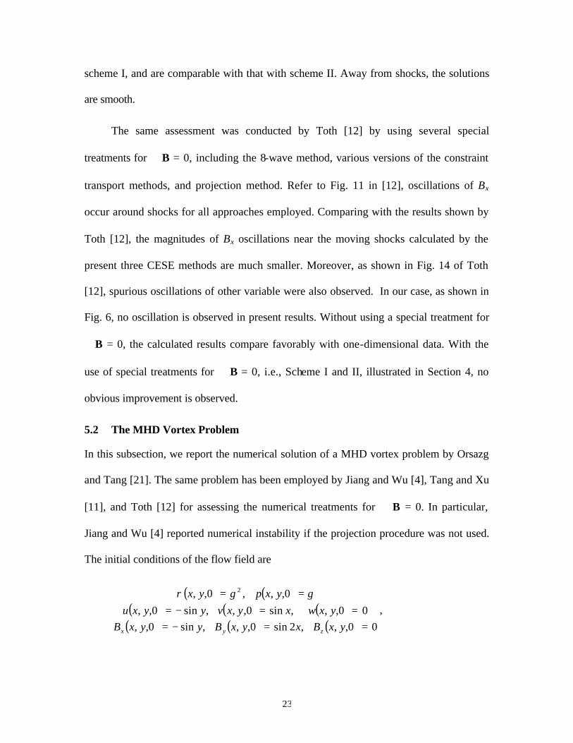
5.2 The MHD Vortex Problem

In this subsection, we report the numerical solution of a MHD vortex problem by Orsazg

and Tang [21]. The same problem has been employed by Jiang and Wu [4], Tang and Xu

[11], and Toth [12] for assessing the numerical treatments for ∇⋅B = 0. In particular,

Jiang and Wu [4] reported numerical instability if the projection procedure was not used.

The initial conditions of the flow field are

( ) ( )( ) ( ) ( )

( ) ( ) ( ) 00,,,2sin0,,,sin0,,00,,,sin0,,,sin0,,

0,,,0,, 2

==−===−=

==

yxBxyxByyxByxwxyxvyyxu

yxpyx

zyx

γγρ,

24

where the specific heat ratio 35=γ . The computational domain is [ ] [ ]ππ 2,02,0 × .

Periodic boundary condition is imposed on boundaries in both x- and y-directions. We

use a uniform mesh of 193×193 grid nodes. The same mesh was used by Jiang and Wu [4]

and Tang and Xu [11].

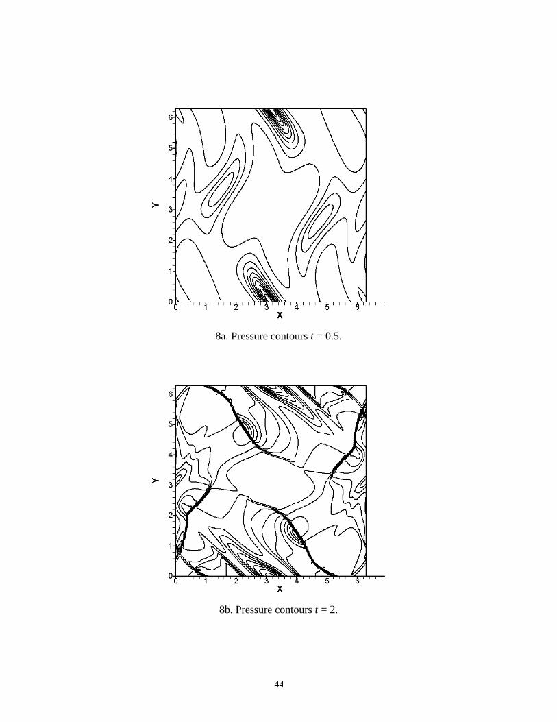
Figs. 8 shows the pressure contours of the present CESE results at t = 0.5, 2, and 3,

respectively. The results here are calculated by using the original CESE method.

Although not shown, the results calculated by using Schemes I and II are virtually the

same in these contour plots. To assess the accuracy of the present results, the employed

contour levels are exactly the same as that used by Jiang and Wu [4], i.e., 12 equally

spaced contour levels ranging from 1.0 to 5.8 for t = 0.5, from 0.14 to 6.9 for t = 2, and

from 0.36 to 6.3 for t = 3. Although not shown in the present paper, side-by-side

comparisons between the present results and Jiang and Wu’s results showed no obvious

difference.

For quantitative details of the calculated results, Fig. 9 shows the pressure profiles

along the line of y = 0.625π at time t = 0.5, 2 and 3, calculated by using the three CESE

schemes: the original scheme and the extended schemes I and II. For t = 0.5, there is no

difference between the results by the three schemes. At t = 2, result by Scheme II showed

a more pronounced gradient near x = 5.5. For t = 3, small differences could be discerned

on the left end of the plot. In Fig. 9c, result reported by Tang and Xu [11] is also plotted.

No obvious difference can be observed between their results and the present results by

the original CESE scheme and Scheme I.

25

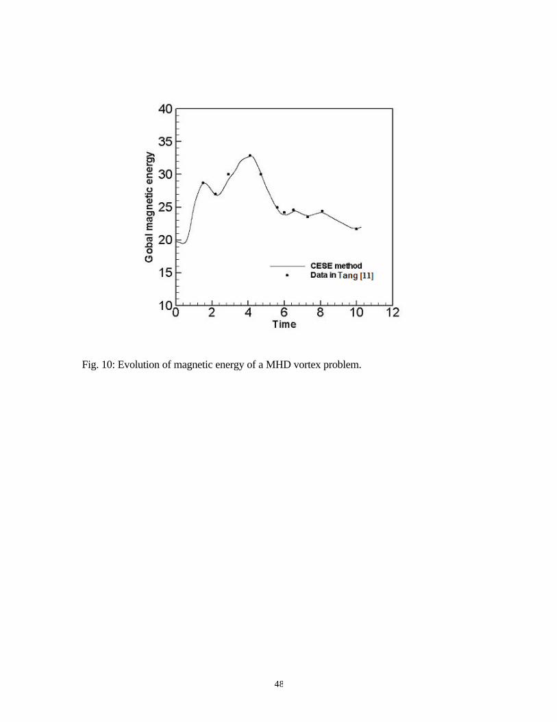
We remark that in scheme II, there is no damping treatment for discontinuity in

calculating the first-order derivatives xBx ∂∂ and yB y ∂∂ . Moreover, the mesh stencil

for calculating xB , yB , xBx ∂∂ , and yB y ∂∂ are larger than that the one (the original

CESE method) used for the rest of unknowns due to the use of SSE and SCE. Figure 10

shows time history of the magnetic energy of the whole flow field. Solid line is the result

from the original CESE method, and dots are Tang and Xu’s results in [11].

To further investigate the capability of the CESE method for ∇⋅B = 0, we adopt the

projection method and solve the Possion equation at every time step,

∇2φ + ∇⋅B = 0, (5.1)

where B is obtained from the CESE method described in Section 3. According to the

mesh arrangement shown in Fig. 1, Eqn. (5.1) is discritized as,

( ) ( )( ) kj

kjkjkjkjkjkj

yx ,221,,21,

2,21,,21

2

2

2

2B⋅∇−=

∆

+−+

∆

+− −+−+ φφφφφφ. (5.2)

An implicit solver is employed to solve the above equation, and the magnetic field B is

updated by,

φ∇+= BB c . (5.3)

The updated Bc is then used to march the flow solution to the next time step. Fig. 11

shows pressure profiles along y = 0.625π at t = 3 with and without the projection

procedure. We observe no obvious improvement by employing the projection procedure.

26

6. Conclusions

In this paper, we report the extension of the CESE method for solving the ideal MHD

equations in two-spatial dimensions with emphasis on satisfying the ∇⋅B = 0 constraint.

Three numerical treatments are developed (i) a simple algebraic adjustment of n

kj

x

xB

,

∂∂

and n

kj

y

yB

,

∂

∂after each time marching step to satisfy ∇⋅B = 0, (ii) an extended CESE

method based on the constraint-transport method to calculate the magnetic field, and (iii)

a projection method by coupling a Poisson solver with the original CESE method. To

demonstrate the capabilities of the CESE methods, two benchmark problems are

calculated and compared with the previously published results, including a rotated MHD

shock tube problem and a MHD vortex problem. All present results produced by the new

CESE schemes compare favorably with the previous results. Moreover, we demonstrate

that the original CESE method could be directly used to calculate the MHD equations

without any difficulty. For the benchmark problems, the results are as accurate as that

produced by using sophisticated special treatments.

References

1. M. Brio and C. C. Wu, An upwind difference scheme for the equations of ideal

magnetohydrodynamics, Journal of Computational Physics, 75, 400-422 (1988).

2. L. Zachary, A. Malagoli and P. A. Colella, A high-order Godunov method for

multidimensional ideal magnetohydrodynamics, SIAM Journal of Scientific

Computation, 15, 263-285, (1994).

27

3. R. S. Myong and P. L. Roe, On Godunov type schemes for magnetohydrodynamics,

Journal of Computational Physics, 147, 545-564 (1998).

4. G. -S. Jiang, C. C. Wu, A high-order WENO finite difference scheme for the

equations of ideal magneto-hydrodynamics, Journal of Computational Physics, 150,

561-594 (1999).

5. J .P. Brackbill and D.C. Barnes, The effect of nonzero B⋅∇ on the numerical

solution of the magnetohydrodynamic equations, Journal of Computational Physics,

35, 426-430 (1980).

6. K. G. Powell, An approximate Riemann solver for magneto-hydro-dynamics, ICASE

Report 94-24 (1994).

7. C .R. Evans, and J. F. Hawley, Simulation of magnetohydrodynamic flows: a

constrained transport Method, Astrophys. J., 332, 659-677 (1988).

8. W. Dai, and P. R. Woodward, A simple finite difference scheme for multidimensional

magnetohydrodanamical equations, Journal of Computational Physics, 142, 331-369

(1998).

9. D. S. Balsara and D. S, Spice, A staggered mesh algorithm using high order Godunov

fluxes to ensure solenoidal magnetic fields in magnetohydrodynamic simulations,

Journal of Computational Physics, 149, 270-292 (1999).

10. D. Ryu, F. T. Miniati, W. Jones and A. Frank, A Divergence-free upwind code for

multidimensional magnetohydrodynamic flows, Astrophys. J., 509, 244-255 (1998).

11. H. -Z. Tang and K. Xu, A high-order gas-kinetic method for multidimensional ideal

magnetohydrodynamics, Journal of Computational Physics, 165, 69-88(2000).

28

12. G. Tóth, The constraint 0=⋅∇ B in shock capturing magneto-hydrodynamics codes,

Journal of Computational Physics, 161, 605-652 (2000).

13. P. Londrillo and L. Del Zanna, On the divergence-free condition in Godunov-type

schemes for ideal magnetohydrodynamics: the upwind constrained transport method,

Journal of Computational Physics, 195, 17-48 (2004).

14. P. R. Peyrard and P. Villedieu, A Roe scheme for ideal MHD equations on 2D

adaptively refined triangular grids, Journal of Computational Physics, 150, 373-393

(1999).

15. S.C. Chang and W. M. To, A new numerical framework for solving conservation

laws – the method of space-time conservation element and solution element, NASA

TM 104498 (1991).

16. S. C. Chang, The method of space-time conservation element and solution element–a

new approach for solving the Navier-Stokes and the Euler Equations, Journal of

Computational Physics, 119, 295-324 (1995).

17. S. C. Chang, X. Y. Wang and C.Y. Chow, The space-time conservation eleme nt and

solution element method: a new high-resolution and genuinely multidimensional

paradigm for solving conservation laws, Journal of Computational Physics, 156, 89-

136 (1999).

18. X. Y. Wang and S. C. Chang, A 2D non-splitting unstructured triangular mesh Euler

solver based on the space-time conservation element and solution element method,

Computational Fluid Dynamics Journal, 8, 309-325 (1999).

29

19. Z.C. Zhang, S. T. Yu, and S. C. Chang, A space-time conservation element and

solution element method for solving the two- and three-dimensional unsteady Euler

equations using quadrilateral and hexahedral meshes, Journal of Computational

Physics, 175, 168-199 (2002).

20. M.J. Zhang, S. C. Lin, S. T. Yu, S. C. Chang and I. Blankson, Application of the

space-time conservation element and solution element method to the ideal

magnetohydrodynamics equations, AIAA paper 2002-3888, (2002).

21. A. Orszag, and C. M. Tang, Small-scale structure of two-dimensional

magnetohydrodynamic turbulence, Journal of Fluid Mechanics, 90, 129-145 (1979).

30

Appendix: Jacobian Matrixes

( ) ( ) ( ) ( ) ( ) ( )

−−−−

−−−

−

−−−−−−

−−−−−−−+−

+−

=∂∂=

uwBBwBuB

uvBBvBuB

AAAAAAAABBuwuw

BBuvuv

BBBwvuwvu

xzxz

xyxy

xz

xy

zyx

000

000

00000000

000000

2211132

12

300000010

87654321

222

ρρρ

ρρρ

γγγγγγγγγ

UFJx

(A.1)

where

ρ

ργ

ργ

γρ

γ

zyx

xzy

wBvBB

Bu

BBuwvuu

ueA

++

++−

+++−+−=222

2221 22

2)()1(

, (A.2a)

ργ

ργγ

γρ

γ222

2222 22

2)(

21

)1(23 xzy BBB

wvue

A −+−

−+−

+−+= , (A.2b)

ργ yx BB

uvA −−= )1(3 , (A.2c)

ργ zx BB

uwA −−= )1(4 , (A.2d)

uA γ=5 , (A.2e)

( )zyx wBvBuBA +−−= γ6 , (A.2f)

( ) yx uBvBA γ−+−= 27 , (A.2g)

31

and

( ) zx uBwBA γ−+−= 28 . (A.2h)

Matrix

( ) ( ) ( ) ( ) ( )

−−−

−

−−

−−−

−−−−−+−

+−

−−

=∂∂

=

vwBBwBvB

uvBBvBuB

BBBBBBBBBBvwvw

BBBwvuwuv

BBuvuv

yzyz

xyxy

yz

zyx

xy

y

000

00000000

000

000

211312

12

300000000100

87654321

222

ρρρ

ρρρ

γγγγγγγγγ

γγ

UG

J

(A.3)

where

ρ

ργ

ργ

γρ

γ

zxy

yzx

wBuBB

Bu

BBvwvuv

veB

++

++−

+++−+−=222

2221 22

2)()1(

, (A.4a)

ργ yxBB

uvB −−= )1(2 , (A.4b)

ργ

ργγ

γρ

γ222

2223 22

2)(

21

)1(23 yzx BBB

wuve

B −+−

−+−

+−+= , (A.4c)

ργ zyBB

vwB −−= )1(4 , (A.4d)

vB γ=5 , (A.4e)

32

( ) yx uBvBB −−= γ26 , (A.4f)

( )zxy wBuBvBB +−−= γ7 , (A.4g)

and

( ) zy vBwBB γ−+−= 28 . (A.4h)

33

List of Figure Captions

Fig. 1: Definition of space-time mesh for a two-dimensional problem.

Fig. 2: Grid arrangement in space-time domain.

Fig. 3: Definition of Special SE and CE for a inherent constrained-transport scheme.

Fig. 4: Relation between x-y coordinates and ξ-η coordinates. Rectangle OABC is the

computational domain.

Fig. 5: Solution to a shock tube, Solid lines stand for one-dimensional results by Toth

[12], dots for present results.

5a. Density.

5b. Pressure.

5c. Velocity component Uξ.

5d. Velocity component Uη.

5e. Magnetic field component Bη.

Fig. 6: Comparison between different CESE schemes for a MHD shock tube problem. 6a. Profiles of P

6b. Profiles of Bη.

Fig. 7: Profiles of Bξ for a MHD shock tube problem from different CESE schemes.

Fig. 8: Pressure contours of a MHD vortex problem by the original CESE scheme.

8a. Pressure contours t = 0.5.

8b. Pressure contours t = 2.

8c. Pressure contours t = 3.

Fig. 9: Pressure profile of a MHD vortex problem along line y = 0.625π.

34

9a. Pressure profile at t = 0.5.

9b. Pressure profile t = 2.

9c. Pressure profile t = 3.

Fig. 10: Evolution of magnetic energy of a MHD vortex problem.

Fig. 11: Comparison between CESE method with and without a projection procedure for

maintaining ∇⋅B = 0.

35

Fig. 1: Definition of space-time mesh for a two-dimensional problem.

36

Fig. 2: Grid arrangement in space-time domain.

37

Fig. 3: Definition of Special SE and CE for a inherent constrained-transport scheme.

38

Fig. 4: Relation between x-y coordinates and ξ-η coordinates. Rectangle OABC is the

computational domain.

39

5a. Pressure.

5b. Density.

40

5c. Velocity component Uξ.

5d. Velocity component Uη.

41

5e. Magnetic field component Bη.

Fig. 5: Solution to shock tube B. Solid lines stand for one-dimensional results by Toth

[12], dots for present results.

42

6b. Profiles of P

6b. Profiles of Bη

Fig. 6: Comparison between different CESE schemes for a MHD shock tube problem.

43

Fig. 7: Profiles of Bξ for a MHD shock tube problem with different CESE schemes.

44

8a. Pressure contours t = 0.5.

8b. Pressure contours t = 2.

45

8c. Pressure contours t = 3.

.

Fig.8: Pressure contours of a MHD vortex problem by the original CESE scheme.

46

9a. Pressure profile at t = 0.5.

9b. Pressure profile t = 2.

47

9c. Pressure profile t = 3.

Fig. 9: Pressure profile of a MHD vortex problem along line y = 0.625π.

48

Fig. 10: Evolution of magnetic energy of a MHD vortex problem.

49

Fig. 11: Comparison between CESE method with and without a projection procedure for

maintaining ∇⋅B = 0.