Solving ordinary differential equationson the Infinity Computer

by working with infinitesimals numerically∗

Yaroslav D. Sergeyev†

Dipartimento di Elettronica, Informatica e Sistemistica,Universita della Calabria,87030 Rende (CS) – Italy

tel./fax: +39 0984 494855http://wwwinfo.deis.unical.it/∼yaroyaro@si.deis.unical.it

Abstract

There exists a huge number of numerical methods that iteratively con-struct approximations to the solution y(x) of an ordinary differential equation(ODE) y′(x) = f(x, y) starting from an initial value y0 = y(x0) and usinga finite approximation step h that influences the accuracy of the obtained ap-proximation. In this paper, a new framework for solving ODEs is presentedfor a new kind of a computer – the Infinity Computer (it has been patentedand its working prototype exists). The new computer is able to work numer-ically with finite, infinite, and infinitesimal numbers giving so the possibilityto use different infinitesimals numerically and, in particular, to take advan-tage of infinitesimal values of h. To show the potential of the new frameworka number of results is established. It is proved that the Infinity Computer isable to calculate derivatives of the solution y(x) and to reconstruct its Tay-lor expansion of a desired order numerically without finding the respectivederivatives analytically (or symbolically) by the successive derivation of theODE as it is usually done when the Taylor method is applied. Methods usingapproximations of derivatives obtained thanks to infinitesimals are discussedand a technique for an automatic control of rounding errors is introduced.Numerical examples are given.

Key Words: Ordinary differential equations, numerical infinitesimals, combiningfinite and infinitesimal approximation steps, Infinity Computer.

∗This study was supported by the Ministry of Education and Science of Russian Federation,project 14.B37.21.0878. The author thanks anonymous reviewers for their useful suggestions.

†Yaroslav D. Sergeyev, Ph.D., D.Sc., is Distinguished Professor at the University of Calabria,Rende, Italy. He is also Full Professor (part-time contract) at the N.I. Lobatchevsky State University,Nizhni Novgorod, Russia and Affiliated Researcher at the Institute of High Performance Computingand Networking of the National Research Council of Italy.

1

1 Introduction

The number of applications in physics, mechanics, and engineering where it isnecessary to solve numerically ordinary differential equations (ODEs) with a giveninitial value is really enormous. Since many ordinary differential equations cannotbe solved analytically, people use numerical algorithms1 for finding approximatesolutions (see [3, 4, 14, 27]). In this paper, we want to approximate the solutiony(x), x ∈ [a, b], of the initial value problem (also called the Cauchy problem) fora differential equation

y′(x) = f(x, y), y(x0) = y0, x0 = a, (1)

where a and b are finite numbers and y(x0) = y0 is called the initial condition.We suppose that f(x, y) is given by a computer procedure. Since very often inscientific and technical applications it can happen that the person who wants tosolve (1) is not the person who has written the code for f(x, y), we suppose thatthe person solving (1) does not know the structure of f(x, y), i.e., it is a black boxfor him/her.

In the literature, there exist numerous numerical algorithms constructing a se-quence y1, y2, y3, . . . approximating the exact values y(x1), y(x2), y(x3), . . . thatthe solution y(x) assumes at points x1, x2, x3, . . . (see [4,13,17]). The explicit Eu-ler algorithm is the simplest among explicit methods for the numerical integrationof ODEs. It uses the first two terms of the Taylor expansion of y(x) constructingso the linear approximation around the point (x0, y(x0)). The (n+1)th step of theEuler algorithm describes how to move from the point xn to xn+1 = xn+h, n > 0,and is executed as follows

yn+1 = yn + hf(xn, yn). (2)

Traditional computers work with finite values of h introducing so errors ateach step of the algorithm. In order to obtain more accurate approximations it isnecessary to decrease the step h increasing so the number of steps of the method(the computations become more expensive). In any case, h always remains finiteand its minimal acceptable value is determined by technical characteristics of eachconcrete computer the method is implemented on. Obviously, the same effects holdfor more sophisticated methods, as well (see [4, 13, 14, 17]). Another approachto solve (1) on a traditional computer is the use of an automatic differentiationsoftware executing pre-processing of (1) (see [12] and references given therein).

In this paper, we introduce a new numerical framework for solving ODEs re-lated to the usage of a new kind of computer – the Infinity Computer (see [31, 33,37]). It is able to work numerically with finite, infinite, and infinitesimal quanti-ties. The Infinity Computer is based on an applied point of view (see [30, 33, 39])

1There exist also symbolic techniques but they are not considered in this paper dedicated tonumerical computations.

2

on infinite and infinitesimal numbers. In order to see the place of the new ap-proach in the historical panorama of ideas dealing with infinite and infinitesimal,see [21, 22, 36, 38, 43]. The new methodology has been successfully applied forstudying numerical differentiation and optimization (see [8, 35, 40, 48]), fractals(see [32, 34, 42, 45]), percolation (see [16, 45]), Euclidean and hyperbolic geome-try (see [23, 29]), the first Hilbert problem and Turing machines (see [38, 43, 44]),cellular automata (see [9]), infinite series (see [36, 41, 47]), functions and theirderivatives that can assume infinite and infinitesimal values (see [36]), etc.

With respect to the initial value problem (1), the possibility to work numericallywith infinitesimals allows us to use numerical infinitesimal values of h. It is provedthat under reasonable conditions the Infinity Computer is able to calculate exactvalues of the derivatives of y(x) and to reconstruct its Taylor expansion with adesired accuracy by using infinitesimal values of h without finding the respectivederivatives analytically (or symbolically) by the successive derivation of (1) as it isusually done when the Taylor method is applied.

The rest of the paper is organized as follows. Section 2 briefly presents thenew computational methodology. Section 3 introduces the main theoretical resultsand describes how derivatives of y(x) can be calculated numerically on the InfinityComputer. Section 4 introduces a variety of examples of the usage of infinitesimalsfor ODEs numerical solving. First, it presents two simple iterative methods. Then,it describes a technique that can be used to obtain approximations of derivativesof the solution y(x) at the point xn+1 using infinitesimals and the informationobtained at the point xn. Finally, a technique for an automatic control of roundingerrors that can occur during evaluation of f(x, y) is introduced. Through the paper,theoretical results are illustrated by numerical examples.

2 A fast tour to the new computational methodology

Numerous trials have been done during the centuries in order to evolve existingnumeral systems2 in such a way that infinite and infinitesimal numbers could beincluded in them (see [2,5,7,19,20,25,28,46]). Particularly, in the early history ofthe calculus, arguments involving infinitesimals played a pivotal role in the deriva-tion developed by Leibniz and Newton (see [19, 25]). The notion of an infinites-imal, however, lacked a precise mathematical definition and in order to provide amore rigorous foundation for the calculus, infinitesimals were gradually replacedby the d’Alembert-Cauchy concept of a limit.

Since new numeral systems appear very rarely, in each concrete historical pe-riod their importance for Mathematics is very often underestimated (especially by

2We are reminded that a numeral is a symbol or group of symbols that represents a number. Thedifference between numerals and numbers is the same as the difference between words and the thingsthey refer to. A number is a concept that a numeral expresses. The same number can be representedby different numerals. For example, the symbols ‘7’, ‘seven’, and ‘VII’ are different numerals, butthey all represent the same number.

3

pure mathematicians). In order to illustrate their importance, let us remind theRoman numeral system that does not allow one to express zero and negative num-bers. In this system, the expression III-X is an indeterminate form. As a result,before appearing the positional numeral system and inventing zero (by the way, thesecond event was several hundred years later with respect to the first one) math-ematicians were not able to create theorems involving zero and negative numbersand to execute computations with them.

There exist numeral systems that are even weaker than the Roman one. Theyseriously limit their users in executing computations. Let us recall a study pub-lished recently in Science (see [11]) that describes a primitive tribe – Piraha –living in Amazonia. These people use a very simple numeral system for counting:one, two, many. For Piraha, all quantities larger than two are just ‘many’ and suchoperations as 2+2 and 2+1 give the same result, i.e., ‘many’. Using their weaknumeral system Piraha are not able to see, for instance, numbers 3, 4, 5, and 6, toexecute arithmetical operations with them, and, in general, to say anything aboutthese numbers because in their language there are neither words nor concepts forthat.

In the context of the present paper, it is very important that the weakness ofPiraha’s numeral system leads them to such results as

‘many’ + 1 = ‘many’, ‘many’ + 2 = ‘many’, (3)

which are very familiar to us in the context of views on infinity used in the tradi-tional calculus

∞+ 1 = ∞, ∞+ 2 = ∞. (4)

The arithmetic of Piraha involving the numeral ‘many’ has also a clear similaritywith the arithmetic proposed by Cantor for his Alephs3:

ℵ0 + 1 = ℵ0, ℵ0 + 2 = ℵ0, ℵ1 + 1 = ℵ1, ℵ1 + 2 = ℵ1. (5)

Thus, the modern mathematical numeral systems allow us to distinguish alarger quantity of finite numbers with respect to Piraha but give results that aresimilar to those of Piraha when we speak about infinite numbers. This observationleads us to the following idea: Probably our difficulties in working with infinity isnot connected to the nature of infinity itself but is a result of inadequate numeralsystems that we use to work with infinity, more precisely, to express infinite num-bers.

Let us compare the usage of numeral systems in Mathematics emphasizing dif-ferences that hold when one works, on the one hand, with finite quantities and, on

3This similarity becomes even more pronounced if one considers another Amazonian tribe –Munduruku (see [26]) – who fail in exact arithmetic with numbers larger than 5 but are able tocompare and add large approximate numbers that are far beyond their naming range. Particularly,they use the words ‘some, not many’ and ‘many, really many’ to distinguish two types of largenumbers using the rules that are very similar to ones used by Cantor to operate with ℵ0 and ℵ1,respectively.

4

the other hand, with infinities and infinitesimals. In our every day activities withfinite numbers the same finite numerals are used for different purposes (e.g., thesame numeral 4 can be used to express the number of elements of a set and to in-dicate the position of an element in a finite sequence). When we face the necessityto work with infinities or infinitesimals, the situation changes drastically. In fact,in this case different symbols are used to work with infinities and infinitesimals indifferent situations:

• ∞ in standard Analysis;

• ω for working with ordinals;

• ℵ0,ℵ1, ... for dealing with cardinalities;

• non-standard numbers using a generic infinitesimal h in non-standard Anal-ysis, etc.

In particular, since the mainstream of the traditional Mathematics very oftendoes not pay any attention to the distinction between numbers and numerals (inthis occasion it is necessary to recall constructivists who studied this issue), manytheories dealing with infinite and infinitesimal quantities have a symbolic (not nu-merical) character. For instance, many versions of the non-standard Analysis aresymbolic, since they have no numeral systems to express their numbers by a finitenumber of symbols (the finiteness of the number of symbols is necessary for orga-nizing numerical computations). Namely, if we consider a finite n than it can betaken n = 5, or n = 103 or any other numeral used to express finite quantities andconsisting of a finite number of symbols. In contrast, if we consider a non-standardinfinite m then it is not clear which numerals can be used to assign a concrete valueto m.

Analogously, in non-standard Analysis, if we consider an infinitesimal h then itis not clear which numerals consisting of a finite number of symbols can be used toassign a value to h and to write h = ... In fact, very often in non-standard Analysistexts, a generic infinitesimal h is used and it is considered as a symbol, i.e., onlysymbolic computations can be done with it. Approaches of this kind leave unclearsuch issues, e.g., whether the infinite 1/h is integer or not or whether 1/h is thenumber of elements of an infinite set. Another problem is related to comparisonof values. When we work with finite quantities then we can compare x and y ifthey assume numerical values, e.g., x = 4 and y = 6 then, by using rules of thenumeral system the symbols 4 and 6 belong to, we can compute that y > x. If onewishes to consider two infinitesimals h1 and h2 then it is not clear how to comparethem because numeral systems that can express infinitesimals are not provided bynon-standard Analysis techniques.

The approach developed in [30, 33, 39] proposes a numeral system that usesthe same numerals for several different purposes for dealing with infinities andinfinitesimals: in Analysis for working with functions that can assume different in-finite, finite, and infinitesimal values (functions can also have derivatives assuming

5

different infinite or infinitesimal values); for measuring infinite sets; for indicatingpositions of elements in ordered infinite sequences; in probability theory, etc. It isimportant to emphasize that the new numeral system avoids situations of the type(3)–(5) providing results ensuring that if a is a numeral written in this system thenfor any a (i.e., a can be finite, infinite, or infinitesimal) it follows a+ 1 > a.

The new numeral system works as follows. A new infinite unit of measure ex-pressed by the numeral ¬ called grossone is introduced as the number of elementsof the set, N, of natural numbers. Concurrently with the introduction of grossonein the mathematical language all other symbols (like ∞, Cantor’s ω, ℵ0,ℵ1, ...,etc.) traditionally used to deal with infinities and infinitesimals are excluded fromthe language because grossone and other numbers constructed with its help notonly can be used instead of all of them but can be used with a higher accuracy.Grossone is introduced by describing its properties postulated by the Infinite UnitAxiom (see [33, 39]) added to axioms for real numbers (similarly, in order to passfrom the set, N, of natural numbers to the set, Z, of integers a new element – zeroexpressed by the numeral 0 – is introduced by describing its properties).

The new numeral ¬ allows us to construct different numerals expressing differ-ent infinite and infinitesimal numbers and to execute computations with them. Asa result, in Analysis, instead of the usual symbol ∞ used in series and integrationdifferent infinite and/or infinitesimal numerals can be used (see [36,41,47]). Inde-terminate forms are not present and, for example, the following relations hold for¬ and ¬−1 (that is infinitesimal), as for any other (finite, infinite, or infinitesimal)number expressible in the new numeral system

0 · ¬ = ¬ · 0 = 0, ¬ − ¬ = 0,¬

¬= 1, ¬0 = 1, 1¬ = 1, 0¬ = 0, (6)

0 · ¬−1 = ¬−1 · 0 = 0, ¬−1 > 0, ¬−2 > 0, ¬−1 − ¬−1 = 0,

¬−1

¬−1 = 1,¬−2

¬−2 = 1, (¬−1)0 = 1, ¬ · ¬−1 = 1, ¬ · ¬−2 = ¬−1.

The new approach gives the possibility to develop a new Analysis (see [36])where functions assuming not only finite values but also infinite and infinitesimalones can be studied. For all of them it becomes possible to introduce a new notionof continuity that is closer to our modern physical knowledge. Functions assumingfinite and infinite values can be differentiated and integrated.

Example 1. The function f(x) = x2 has the first derivative f ′(x) = 2x andboth f(x) and f ′(x) can be evaluated at infinite and infinitesimal x. Thus, forinfinite x = ¬ we obtain infinite values

f(¬) = ¬2, f ′(¬) = 2¬

and for infinitesimal x = ¬−1 we have infinitesimal values

f(¬−1) = ¬−2, f ′(¬−1) = 2¬−1.

6

If x = 5¬ − 10¬−1 then we have

f(¬−1) = (5¬ − 10¬−1)2 = 25¬2 − 100 + 100¬−2,

f ′(¬−1) = 10¬ − 20¬−1.

We can also work with functions defined by formulae including infinite and in-finitesimal numbers. For example, the function f(x) = 1

¬x2+¬x has a quadratic

term infinitesimal and the linear one infinite. It has the first derivative f ′(x) =2¬x+ ¬. For infinite x = 3¬ we obtain infinite values

f(¬) = 3¬2 + 9¬, f ′(¬) = ¬ + 6

and for infinitesimal x = ¬−1 we have

f(¬−1) = 1 + ¬−3, f ′(¬−1) = ¬ + 2¬−2. 2

By using the new numeral system it becomes possible to measure certain infi-nite sets and to see, e.g., that the sets of even and odd numbers have ¬/2 elementseach. The set, Z, of integers has 2¬+1 elements (¬ positive elements, ¬ negativeelements, and zero). Within the countable sets and sets having cardinality of thecontinuum (see [21, 38, 39]) it becomes possible to distinguish infinite sets havingdifferent number of elements expressible in the numeral system using grossone andto see that, for instance,

¬

2< ¬ − 1 < ¬ < ¬ + 1 < 2¬ + 1 < 2¬2 − 1 < 2¬2 < 2¬2 + 1 <

2¬2 + 2 < 2¬ − 1 < 2¬ < 2¬ + 1 < 10¬ < ¬¬ − 1 < ¬¬ < ¬¬ + 1.

The Infinity Computer used in this paper for solving the problem (1) workswith numbers having finite, infinite, and infinitesimal parts. To represent themin the computer memory records similar to traditional positional numeral systemscan be used (see [33, 37]). To construct a number C in the new numeral positionalsystem4 with base ¬, we subdivide C into groups corresponding to powers of ¬:

C = cpm¬pm + . . .+ cp1¬p1 + cp0¬p0 + cp−1¬p−1 + . . .+ cp−k¬p−k . (7)

4At the first glance the numerals (7) can remind numbers from the Levi-Civita field (see [20]) thatis a very interesting and important precedent of algebraic manipulations with infinities and infinites-imals. However, the two mathematical objects have several crucial differences. They have beenintroduced for different purposes by using two mathematical languages having different accuraciesand on the basis of different methodological foundations. In fact, Levi-Civita does not discuss thedistinction between numbers and numerals. His numbers have neither cardinal nor ordinal proper-ties; they are build using a generic infinitesimal and only its rational powers are allowed; he usessymbol ∞ in his construction; there is no any numeral system that would allow one to assign numer-ical values to these numbers; it is not explained how it would be possible to pass from d a genericinfinitesimal h to a concrete one (see also the discussion above on the distinction between numbersand numerals). In no way the said above should be considered as a criticism with respect to resultsof Levi-Civita. The above discussion has been introduced in this text just to underline that we are infront of two different mathematical tools that should be used in different mathematical contexts.

7

Then, the record

C = cpm¬pm . . . cp1¬p1cp0¬p0cp−1¬p−1 . . . cp−k¬p−k (8)

represents the number C, where all numerals ci = 0, they belong to a traditionalnumeral system and are called grossdigits. They express finite positive or negativenumbers and show how many corresponding units ¬pi should be added or sub-tracted in order to form the number C. Note that in order to have a possibility tostore C in the computer memory, values k and m should be finite.

Numbers pi in (8) are sorted in the decreasing order with p0 = 0

pm > pm−1 > . . . > p1 > p0 > p−1 > . . . p−(k−1) > p−k.

They are called grosspowers and they themselves can be written in the form (8).In the record (8), we write ¬pi explicitly because in the new numeral positionalsystem the number i in general is not equal to the grosspower pi. This gives thepossibility to write down numerals without indicating grossdigits equal to zero.

The term having p0 = 0 represents the finite part of C because, due to (6),we have c0¬

0 = c0. The terms having finite positive grosspowers represent thesimplest infinite parts of C. Analogously, terms having negative finite grosspowersrepresent the simplest infinitesimal parts of C. For instance, the number ¬−1 = 1

¬mentioned above is infinitesimal. Note that all infinitesimals are not equal to zero.Particularly, 1

¬> 0 because it is a result of division of two positive numbers.

A number represented by a numeral in the form (8) is called purely finite ifit has neither infinite not infinitesimals parts. For instance, 2 is purely finite and2 + 3¬−1 is not. All grossdigits ci are supposed to be purely finite. Purely finitenumbers are used on traditional computers and for obvious reasons have a specialimportance for applications.

All of the numbers introduced above can be grosspowers, as well, giving thus apossibility to have various combinations of quantities and to construct terms havinga more complex structure. However, in this paper we consider only purely finitegrosspowers. Let us give an example of multiplication of two infinite numbers Aand B of this kind (for a comprehensive description see [33, 37]).

Example 2. Let us consider numbers A and B, where

A = 14.3¬56.25.4¬0, B = 6.23¬31.5¬−4.1.

The number A has an infinite part and a finite one. The number B has an infinitepart and an infinitesimal one. Their product C is equal to

C = B ·A = 89.089¬59.221.45¬52.133.642¬38.1¬−4.1. 2

We conclude this section by emphasizing that there exist different mathemati-cal languages and numeral systems and, if they have different accuracies, it is notpossible to use them together. For instance, the usage of ‘many’ from the languageof Piraha in the record 4 + ‘many’ has no any sense because for Piraha it is not

8

clear what is 4 and for people knowing what is 4 the accuracy of the answer ‘many’is too low. Analogously, the records of the type ¬ + ω, ¬ − ℵ0, ¬/∞, etc. haveno sense because they belong to languages developed for different purposes andhaving different accuracies.

3 Numerical reconstruction of the Taylor expansion of thesolution on the Infinity Computer

Let us return to the problem (1). We suppose that a set of elementary functions(ax, sin(x), cos(x), etc.) is represented at the Infinity Computer by one of theusual ways used in traditional computers (see, e.g. [24]) involving the argumentx, finite constants, and four arithmetical operations. Then the following theoremholds (the world exact in it means: with the accuracy of the computer programmeimplementing f(x, y) from (1)).

Theorem 1 Let us suppose that for the solution y(x), x ∈ [a, b], of (1) there existsthe Taylor expansion (unknown for us) and at purely finite points s ∈ [a, b], thefunction y(s) and all its derivatives assume purely finite values or are equal to zero.Then the Infinity Computer allows one to reconstruct the Taylor expansion for y(x)up to the k-th derivative with exact values of y′(x), y′′(x), y(3)(x), . . . y(k)(x) afterk steps of the Euler method with the step h = ¬−1.

Proof. Let us start to execute on the Infinite Computer steps of the Eulermethod following the rule (2) and using the infinitesimal step h = ¬−1. Since theproblem (1) has been stated using the traditional finite mathematics, x0 is purelyfinite. Without loss of generality let us consider the first k = 4 steps of the Eulermethod (the value k = 4 is sufficient to show the way of reasoning; we shall usethe formulae involved in this case later in a numerical illustration). We obtain

y1 = y0 + ¬−1f(x0, y0), y2 = y1 + ¬−1f(x1, y1), (9)

y3 = y2 + ¬−1f(x2, y2), y4 = y3 + ¬−1f(x3, y3). (10)

The derivatives of the solution y(x) can be approximated in different ways andwith different orders of accuracy. Let us consider approximations (see, e.g., [10])executed by forward differences △j

h, 1 ≤ j ≤ k, with the first order of accuracyand take h = ¬−1 as follows

△k¬−1 =

k∑i=0

(−1)i(ki

)yx0+(k−i)¬−1 . (11)

Then we have

y′(x0) ≈△1

¬−1

¬−1 +O(¬−1

)=

y1 − y0

¬−1 +O(¬−1

), (12)

9

y′′(x0) ≈△2

¬−1

¬−2 +O(¬−1

)=

y0 − 2y1 + y2

¬−2 +O(¬−1

), (13)

y(3)(x0) ≈△3

¬−1

¬−3 +O(¬−1

)=

−y0 + 3y1 − 3y2 + y3

¬−3 +O(¬−1

), (14)

y(4)(x0) ≈△4

¬−1

¬−4 +O(¬−1

)=

y0 − 4y1 + 6y2 − 4y3 + y4

¬−4 +O(¬−1

). (15)

Since due to (1) we can evaluate directly y′(x0) = f(x0, y0), let us start byconsidering the formula (13) (the cases with values of k > 2 are studied by a com-plete analogy). Since x0 is purely finite, then due to our assumptions y′′(x0) is alsopurely finite. This means that y′′(x0) does not contain infinitesimal parts. Formula(13) states that the error we have when instead of y′′(x0) use its approximation

y′′(x0) =△2

¬−1

¬−2 (16)

is of the order ¬−1. The Infinity Computer works in such a way that it collectsdifferent orders of ¬ in separate groups. Thus, △2

¬−1 will be represented in theformat (8)

△2¬−1 = c0¬

0 + c−1¬−1 + c−2¬

−2 + . . .+ c−m2¬−m2 , (17)

where m2 is a finite integer, its value depends on each concrete f(x, y) from (1).Note that (17) cannot contain fractional grosspowers because the step h = ¬−1

having the integer grosspower −1 has been chosen in (9), (10).It follows from (13) and the fact that y′′(x0) is purely finite that y′′(x0) contains

a purely finite part and can contain infinitesimal parts of the order ¬−1 or higher.This means that grossdigits c0 = c−1 = 0, otherwise after division on ¬−2 theestimate y′′(x0) would have infinite parts and this is impossible. Thus y′′(x0) hasthe following structure

y′′(x0) = c−2¬0 + c−3¬

−1 + c−4¬−2 + . . .+ c−m¬−m+2. (18)

It follows from (13) that y′′(x0) can contain an error of the order ¬−1 or higher.Since all the derivatives of y(x) are purely finite at x0 and, in particular, y′′(x0) ispurely finite, the fact that the finite part and infinitesimal parts in (18) are separatedgives us that c−2 = y′′(x0). Thus, in order to have the exact value of y′′(x0) itis sufficient to calculate △2

¬−1 from (18) and to take its grossdigit c−2 that will beequal to y′′(x0).

By a complete analogy the exact values of higher derivatives can be obtainedfrom (12) – (15) and analogous formulae using forward differences (11) to approx-imate the k-th derivative y(k)(x0). It suffices just to calculate △k

¬−1 and to take thegrossdigit c−k that will be equal to the exact value of the derivative y(k)(x0). 2

10

Let us consider an illustrative numerical example. We emphasize that the In-finity Computer solves it numerically, not symbolically, i.e., it is not necessary totranslate the procedure implementing f(x, y) in a symbolic form.

Example 3. Let us consider the problem

y′(x) = x− y, y(0) = 1, (19)

taken from [1]. Its exact solution is

y(x) = x− 1 + 2e−x. (20)

We start by applying formulae (9) to calculate y1 and y2:

y1 = 1 + ¬−1 · (0− 1) = 1− ¬−1,

y2 = 1− ¬−1 + ¬−1(¬−1 − 1 + ¬−1) = 1− 2¬−1 + 2¬−2.

We have now the values y0, y1, and y2. Thus, we can apply formula (13) andcalculate △2

¬−1 as follows

△2¬−1 = y0 − 2y1 + y2 = 1− 2 + 2¬−1 + 1− 2¬−1 + 2¬−2 = 2¬−2.

Thus, c−2 = 2. Let us now verify the obtained result and calculate the exactderivative y′′(0) using (20). Then we have y′′(x) = 2e−x, and y′′(0) = 2, i.e.,c−2 = y′′(0). Note that in this simple illustrative example c−m = 0, m > 2,where m is from (13). In general, this is not the case and c−m = 0 can occur.

Let us proceed and calculate y3 following (10). We have

y3 = 1−2¬−1+2¬−2+¬−1(2¬−1−1+2¬−1−2¬−2) = 1−3¬−1+6¬−2−2¬−3.

It then follows from (14) that

△3¬−1 = −y0 + 3y1 − 3y2 + y3 =

−1+3(1−¬−1)−3(1−2¬−1+2¬−2)+1−3¬−1+6¬−2−2¬−3 = −2¬−3.

We can see that c−3 = −2. The exact derivative obtained from (20) is y(3)(x) =−2e−x. As a consequence, we have y(3)(0) = −2, i.e., c−3 = y(3)(0).

To calculate y(4)(0) we use (10) and have

y4 = 1− 3¬−1 + 6¬−2 − 2¬−3 + ¬−1(3¬−1 − 1 + 3¬−1 − 6¬−2 + 2¬−3) =

1− 4¬−1 + 12¬−2 − 8¬−3 + 2¬−4.

From (15) we obtain

△4¬−1 = y0 − 4y1 + 6y2 − 4y3 + y4 = 1− 4(1− ¬−1) + 6(1− 2¬−1 + 2¬−2)−

−4(1− 3¬−1 + 6¬−2 − 2¬−3) + 1− 4¬−1 + 12¬−2 − 8¬−3 + 2¬−4 =

11

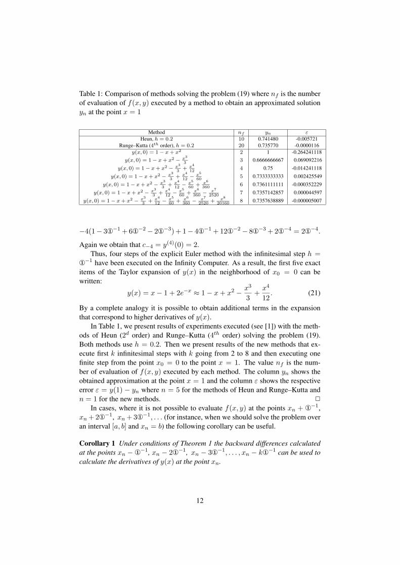
Table 1: Comparison of methods solving the problem (19) where nf is the numberof evaluation of f(x, y) executed by a method to obtain an approximated solutionyn at the point x = 1

Method nf yn εHeun, h = 0.2 10 0.741480 -0.005721

Runge–Kutta (4th order), h = 0.2 20 0.735770 -0.0000116y(x, 0) = 1− x+ x2 2 1 -0.264241118

y(x, 0) = 1− x+ x2 − x3

33 0.6666666667 0.069092216

y(x, 0) = 1− x+ x2 − x3

3+ x4

124 0.75 -0.014241118

y(x, 0) = 1− x+ x2 − x3

3+ x4

12− x5

605 0.7333333333 0.002425549

y(x, 0) = 1− x+ x2 − x3

3+ x4

12− x5

60+ x6

3606 0.7361111111 -0.000352229

y(x, 0) = 1− x+ x2 − x3

3+ x4

12− x5

60+ x6

360− x7

25207 0.7357142857 0.000044597

y(x, 0) = 1− x+ x2 − x3

3+ x4

12− x5

60+ x6

360− x7

2520+ x8

201608 0.7357638889 -0.000005007

−4(1− 3¬−1 +6¬−2 − 2¬−3) + 1− 4¬−1 +12¬−2 − 8¬−3 +2¬−4 = 2¬−4.

Again we obtain that c−4 = y(4)(0) = 2.Thus, four steps of the explicit Euler method with the infinitesimal step h =

¬−1 have been executed on the Infinity Computer. As a result, the first five exactitems of the Taylor expansion of y(x) in the neighborhood of x0 = 0 can bewritten:

y(x) = x− 1 + 2e−x ≈ 1− x+ x2 − x3

3+

x4

12. (21)

By a complete analogy it is possible to obtain additional terms in the expansionthat correspond to higher derivatives of y(x).

In Table 1, we present results of experiments executed (see [1]) with the meth-ods of Heun (2d order) and Runge–Kutta (4th order) solving the problem (19).Both methods use h = 0.2. Then we present results of the new methods that ex-ecute first k infinitesimal steps with k going from 2 to 8 and then executing onefinite step from the point x0 = 0 to the point x = 1. The value nf is the num-ber of evaluation of f(x, y) executed by each method. The column yn shows theobtained approximation at the point x = 1 and the column ε shows the respectiveerror ε = y(1) − yn where n = 5 for the methods of Heun and Runge–Kutta andn = 1 for the new methods. 2

In cases, where it is not possible to evaluate f(x, y) at the points xn + ¬−1,xn+2¬−1, xn+3¬−1, . . . (for instance, when we should solve the problem overan interval [a, b] and xn = b) the following corollary can be useful.

Corollary 1 Under conditions of Theorem 1 the backward differences calculatedat the points xn − ¬−1, xn − 2¬−1, xn − 3¬−1, . . . , xn − k¬−1 can be used tocalculate the derivatives of y(x) at the point xn.

12

Proof. The backward difference (see e.g., [10]) of the order k with h = ¬−1

is calculated as follows

∇k¬−1 =

k∑i=0

(−1)i(ki

)yx0−i¬−1 .

The rest of the proof is completely analogous to the proof of the theorem and is soomitted. 2

Thus, if the region of interest [a, b] from (1) belongs to the region of conver-gence of the Taylor expansion for the solution y(x) around the point x0 then itis not necessary to construct iterative procedures involving several steps with fi-nite values of h and it becomes possible to calculate approximations of the desiredorder by executing only one finite step.

4 Examples of the usage of infinitesimals in the newcomputational framework

The approach introduced in the previous section gives the possibility to constructa variety of new numerical methods for the Infinity Computer by using both in-finitesimal and finite values of h. The general step n of a method of this kind forsolving (1) can be described as follows:

(i) take the point (xn, yn), choose a value kn, and execute kn steps of the Eulermethod starting from xn by using h = ¬−1;

(ii) calculate exact values of y′(x), y′′(x), y(3)(x), . . . , y(kn)(x) at the point(xn, yn) following the rules described in Theorem 1;

(iii) construct the truncated Taylor expansion of the order kn;

(iv) execute a single step from the point xn to xn+1 = xn + hi using the con-structed Taylor expansion and a finite value of hn (steps of the kind hn−¬−1

or hn + ¬−1 can be also used).

The general step described above allows one to construct numerical algorithmsfor solving (1) by executing several iterations of this kind. Many numerical meth-ods (see [4, 14, 27]) can be used as a basis for such developments. Due to the easyway allowing us to calculate exact higher derivatives at the points (xn, yn), meth-ods that use higher derivatives are of the main interest. The fact that to increasethe accuracy it is necessary just to execute one additional infinitesimal step withoutperforming additional finite steps (i.e., the whole work executed at a lower level ofaccuracy is used entirely at a higher level of accuracy) is an additional advantageand suggests to construct adaptive methods (for instance, if one wishes to changethe finite step from h1 to h2 > h1 or h3 < h1 then the same Taylor expansion canbe used in all the cases). A study of such methods will be done in a separate paper.

13

Hereinafter, since the usage of numerical infinitesimals is a new topic, we give anumber of examples showing how the new computational framework can be usedin the context of numerical solving ODEs.

The rest of this section is organized as follows. In the first subsection, wepresent two simple iterative methods using low derivatives (a lower order of deriva-tives is used for expository reasons). In the second subsection, we present a tech-nique that can be used to obtain an additional information with respect to approx-imations of derivatives of the solution. In the last subsection, we discuss howan automatic control of rounding errors can be executed during the evaluation off(x, y) at the points (xn, yn).

4.1 A simple method and possibilities of its improvements

We start by introducing the Method 1 that uses only the first and the second deriva-tives at each iteration to construct the Taylor expansion by applying formulae (9),(12), and (13). Thus, this method at the current point xn executes twice the Eulerstep with h = ¬−1 and then makes the step with a finite value of h by using theobtained Taylor expansion. Therefore, during these three steps (two infinitesimalsteps and one finite step) the function f(x, y) is evaluated twice and only during theinfinitesimals steps. Let us use the number step n to count the executed finite stepsand denote by y(x, z) the Taylor expansion of the solution y(x) calculated by themethod during the infinitesimal steps at the neighborhood of the point z = xn−1.Then, we can calculate yn as yn = y(h, xn−1) with a finite value of h.

Example 4. We test this method on the problem (19) with the finite step h =0.2 (see Table 2). By applying the procedure described above with six digits afterthe dot we have that

y(x, 0) = 1− x+ x2, y1 = y(0.2, 0) = 0.84, (22)

y(x, 0.2) = 0.84− 0.64x+ 0.82x2, y2 = y(0.2, 0.2) = 0.7448,

y(x, 0.4) = 0.7448− 0.3448x+ 0.6724x2, y3 = y(0.2, 0.4) = 0.702736,

y(x, 0.6) = 0.702736−0.102736x+0.551368x2, y4 = y(0.2, 0.6) = 0.704244,

y(x, 0.8) = 0.704244+0.095756x+0.452122x2, y5 = y(0.2, 0.8) = 0.741480.

It can be seen from Table 2 that the results obtained by the new method (seecolumn Method 1.0) for the values yn coincide (see [1]) with the results obtained byapplying the modified Euler’s method (called also Heun’s method) that evaluatesf(x, y) twice at each iteration as the new method does.

As it can be seen from the formulae above, the Method 1 at each point xn pro-vides us not only with the value yn but also with the first and the second derivativesof y(x) at the point (xn, yn). We shall denote them as y′n(xn) and y′′n(xn) where

y′n(xn) = y′(0, xn), y′′n(xn) = y′′(0, xn).

14

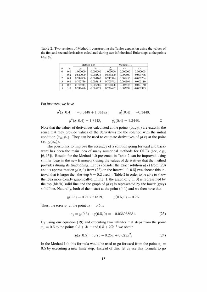
Table 2: Two versions of Method 1 constructing the Taylor expansion using the values ofthe first and second derivatives calculated during two infinitesimal Euler steps at the points(xn, yn)

Method 1.0 Method 1.1n xn yn εn ycn cn εn0 0.0 1.000000 0.000000 1.000000 0.000000 0.0000001 0.2 0.840000 -0.002538 0.839200 0.000800 -0.0017382 0.4 0.744800 -0.004160 0.743344 0.001456 -0.0027043 0.6 0.702736 -0.005113 0.700742 0.001994 -0.0031194 0.8 0.704244 -0.005586 0.701808 0.002436 -0.0031505 1.0 0.741480 -0.005721 0.738682 0.002798 -0.002923

For instance, we have

y′(x, 0.4) = −0.3448 + 1.3448x, y′2(0.4) = −0.3448,

y′′(x, 0.4) = 1.3448, y′′2(0.4) = 1.3448. 2

Note that the values of derivatives calculated at the points (xn, yn) are exact in thesense that they provide values of the derivatives for the solution with the initialcondition (xn, yn). They can be used to estimate derivatives of y(x) at the point(xn, y(xn)).

The possibility to improve the accuracy of a solution going forward and back-ward has been the main idea of many numerical methods for ODEs (see, e.g.,[6, 15]). Results for the Method 1.0 presented in Table 2 can be improved usingsimilar ideas in the new framework using the values of derivatives that the methodprovides during its functioning. Let us consider the exact solution y(x) from (20)and its approximation y(x, 0) from (22) on the interval [0, 0.5] (we choose this in-terval that is larger then the step h = 0.2 used in Table 2 in order to be able to showthe idea more clearly graphically). In Fig. 1, the graph of y(x, 0) is represented bythe top (black) solid line and the graph of y(x) is represented by the lower (grey)solid line. Naturally, both of them start at the point (0, 1) and we then have that

y(0.5) = 0.713061319, y(0.5, 0) = 0.75.

Thus, the error ε1 at the point x1 = 0.5 is

ε1 = y(0.5)− y(0.5, 0) = −0.036938681. (23)

By using our equation (19) and executing two infinitesimal steps from the pointx1 = 0.5 to the points 0.5 + ¬−1 and 0.5 + 2¬−1 we obtain

y(x, 0.5) = 0.75− 0.25x+ 0.625x2. (24)

In the Method 1.0, this formula would be used to go forward from the point x1 =0.5 by executing a new finite step. Instead of this, let us use this formula to go

15

Figure 1: The graph of y(x, 0) is represented by the top (black) solid line and thegraph of y(x) is represented by the lower (grey) solid line (both y(x, 0) and y(x)start at the point (0, 1)); the graph of the function y(x) is shown by the top dashedline; the graph of the function r1(x) is shown by the lower dashed line.

backward from the point x1 = 0.5 to the starting point x0 = 0. Since in (24) xis intended to be a removal from the point x1 = 0.5, we need to take into accountthis fact. The graph of the obtained function

y(x) = 0.75 + 0.25(0.5− x) + 0.625(0.5− x)2 = 1.03125− 0.875x+ 0.625x2

is shown in Fig. 1 by the top dashed line.It can be seen that y(x, 0) from (22) does not coincide with the obtained func-

tion y(x). Let us construct a new quadratic approximation r1(x) oriented on abetter result to be obtained at the point x1 = 0.5. The function r1(x) is built usingcoefficients from both y(x, 0) and y(x) by taking their average with the weights12 and 1

2 (the general way to mix them is, obviously, τ and 1 − τ, 0 < τ < 1) asfollows:

r1(x) = y(0, 0)+1

2(y(0, 0)−y(0))+

1

2(y′(0, 0)+y′(0))x+

1

4(y′′(0, 0)+y′′(0))x2 =

1 +1

2(1− 1.03125) +

1

2(−1− 0.875)x+

1

2(1 + 0.625)x2 =

0.984375− 0.9375x+ 0.8125x2. (25)

In Fig. 1, the graph of the function r1(x) is shown by the lower dashed line. Thefunction r1(x) provides us the value r1(0.5) = 0.718750 and the respective error

ε1 = y(0.5)− r1(0.5) = −0.005688681. (26)

16

that is better than the error ε1 = −0.036938681 from (23) that is obtained bycalculating y(0.5, 0).

The possibility to calculate corrections to approximations opens the doors tovarious modifications. For instance, it is possible to execute two additional in-finitesimal steps at the point x1 = 0.5 using the value r1(0.5) instead of y(0.5, 0).In general, this means that instead of setting yn = y(xn, xn−1) as it is done bythe Method 1.0 we put yn = rn(xn). Obviously, this means that it is necessary toevaluate f(x, y) two times more with respect to the Method 1.0. Otherwise it isalso possible to use the corrected value rn(xn) with the derivatives that have beencalculated for y(xn, xn−1).

Another possibility would be the use of the functions y(x, xn) at each point xn,i.e., to put yn = y(xn, xn−1), and to calculate the global correction following therule

cn = c(xn) = c(xn−1) + rn(xn)− y(xn, xn−1), (27)

starting from the first correction (in our example c(x1) = c(0.5) = 0.031250)

c(x1) = r1(x1)− y(x1, x0).

In this way we can approximate the exact solution y(xn) by the corrected value

ycn = y(xn, xn−1) + c(xn).

In Table 2, results for this algorithm are presented in the column Method 1.1 wherethe error εn is calculated as

εn = y(xn)− ycn.

Notice that the correction obtained at the final point has been calculated usingCorollary 1.

We conclude this subsection by a reminder that Theorem 1 gives us the possi-bility to easily construct higher-order methods. Two methods described above justshow examples of the usage of infinitesimals for building algorithms for solvingODEs.

4.2 Approximating derivatives of the solution

In this subsection, we show how approximations of derivatives at the point xn canbe obtained using the information calculated at the point xn−1. For this purpose,instead of the usage of a finite step h, the steps h− ¬−1 or h+ ¬−1 can be used.To introduce this technique we need to recall the following theorem from [40].

Theorem 2 Suppose that: (i) for a function s(x) calculated by a procedure imple-mented at the Infinity Computer there exists an unknown Taylor expansion in a fi-nite neighborhood δ(z) of a purely finite point z; (ii) s(x), s′(x), s′′(x), . . . s(k)(x)assume purely finite values or are equal to zero at purely finite x ∈ δ(z); (iii) s(x)

17

has been evaluated at a point z + ¬−1 ∈ δ(z). Then the Infinity Computer re-turns the result of this evaluation in the positional numeral system with the infiniteradix ¬ in the following form

s(z + ¬−1) = c0¬0c−1¬

−1c−2¬−2 . . . c−(k−1)¬

−(k−1)c−k¬−k, (28)

where

s(z) = c0, s′(z) = c−1, s′′(z) = 2!c−2, . . . s(k)(z) = k!c−k. (29)

The theorem tells us that if we take a purely finite point z and evaluate on theInfinity Computer s(x) at the point z+¬−1 then from the computed s(z+¬−1) wecan easily extract s(z), s′(z), s′′(z), etc. To apply this theorem to our situation wecan take as s(x) the Taylor expansion for y(x) constructed up to the kth derivativeusing infinitesimal steps ¬−1, 2¬−1, . . . , k¬−1. Then, if we take as z a purelyfinite step h and evaluate on the Infinity Computer s(x) at the point h+ ¬−1 thenwe obtain s(h), s′(h), s′′(h), etc.

For instance, let us take s(x) = s2(x) = y(x, 0), where y(x, 0) is from (22)and s2(x) indicates that we use two derivatives in the Taylor expansion. Then, wehave

s2(0.2 + ¬−1) = 1− (0.2 + ¬−1) + (0.2 + ¬−1)2 = 0.84− 0.6¬−1 + ¬−2.

We have the exact (where the word “exact” again means: with the accuracy of theimplementation of s(x)) values s(0.2) = 0.84, s′(0.2) = −0.6, s′′(0.2) = 1 forthe function s(x). These values can be used to approximate the respective valuesy(0.2), y′(0.2), y′′(0.2) we are interested in. Moreover, we can adaptively obtainan information on the accuracy of our approximations by consecutive improve-ments. If we calculate now y(3)(0) from (14) then we can improve our approxima-tion by setting s(x) = s3(x) where

s3(0.2 + ¬−1) = s2(0.2 + ¬−1)− 1

3(0.2 + ¬−1)3 =

s2(0.2 + ¬−1)− 0.002667− 0.04¬−1 − 0.2¬−2 − 1

3¬−3 =

0.837333− 0.64¬−1 + 0.8¬−2 − 1

3¬−3. (30)

Note, that to obtain this information we have calculated only the additional part ofs3(0.2) taking the rest from the already calculated value s2(0.2).

Analogously, if we calculate now y(4)(0) from (15) then we can improve ourapproximation again by setting s(x) = s4(x) where

s4(0.2 + ¬−1) = s3(0.2 + ¬−1) +1

12(0.2 + ¬−1)4 =

s3(0.2+¬−1)+0.000133+0.002667¬−1+0.02¬−2+0.066667¬−3+1

12¬−4 =

18

0.837466− 0.637333¬−1 + 0.82¬−2 − 0.266667¬−3 +1

12¬−4.

Since we have used the convergent Taylor expansion of the fourth order, the errorsin calculating y(0.2), y′(0.2), and y′′(0.2) are of the orders 5, 4, and 3, respectively.

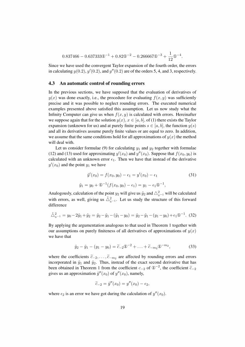
4.3 An automatic control of rounding errors

In the previous sections, we have supposed that the evaluation of derivatives ofy(x) was done exactly, i.e., the procedure for evaluating f(x, y) was sufficientlyprecise and it was possible to neglect rounding errors. The executed numericalexamples presented above satisfied this assumption. Let us now study what theInfinity Computer can give us when f(x, y) is calculated with errors. Hereinafterwe suppose again that for the solution y(x), x ∈ [a, b], of (1) there exists the Taylorexpansion (unknown for us) and at purely finite points s ∈ [a, b], the function y(s)and all its derivatives assume purely finite values or are equal to zero. In addition,we assume that the same conditions hold for all approximations of y(x) the methodwill deal with.

Let us consider formulae (9) for calculating y1 and y2 together with formulae(12) and (13) used for approximating y′(x0) and y′′(x0). Suppose that f(x0, y0) iscalculated with an unknown error ϵ1. Then we have that instead of the derivativey′(x0) and the point y1 we have

y′(x0) = f(x0, y0)− ϵ1 = y′(x0)− ϵ1 (31)

y1 = y0 + ¬−1(f(x0, y0)− ϵ1) = y1 − ϵ1¬−1,

Analogously, calculation of the point y2 will give us y2 and △2¬−1 will be calculated

with errors, as well, giving us △2¬−1 . Let us study the structure of this forward

difference

△2¬−1 = y0−2y1+ y2 = y2− y1−(y1−y0) = y2− y1−(y1−y0)+ϵ1¬

−1. (32)

By applying the argumentation analogous to that used in Theorem 1 together withour assumptions on purely finiteness of all derivatives of approximations of y(x)we have that

y2 − y1 − (y1 − y0) = c−2¬−2 + . . .+ c−m2¬−m2 , (33)

where the coefficients c−2, . . . , c−m2 are affected by rounding errors and errorsincorporated in y1 and y2. Thus, instead of the exact second derivative that hasbeen obtained in Theorem 1 from the coefficient c−2 of ¬−2, the coefficient c−2

gives us an approximation y′′(x0) of y′′(x0), namely,

c−2 = y′′(x0) = y′′(x0)− ϵ2,

where ϵ2 is an error we have got during the calculation of y′′(x0).

19

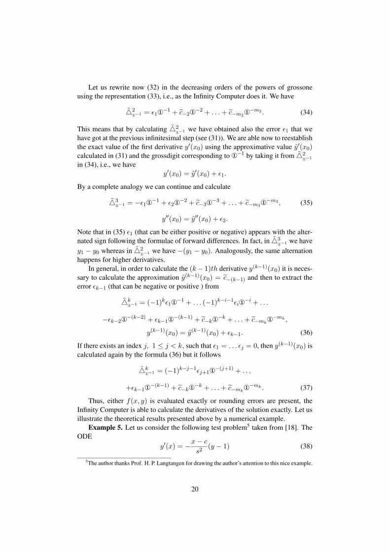
Let us rewrite now (32) in the decreasing orders of the powers of grossoneusing the representation (33), i.e., as the Infinity Computer does it. We have

△2¬−1 = ϵ1¬

−1 + c−2¬−2 + . . .+ c−m2¬−m2 . (34)

This means that by calculating △2¬−1 we have obtained also the error ϵ1 that we

have got at the previous infinitesimal step (see (31)). We are able now to reestablishthe exact value of the first derivative y′(x0) using the approximative value y′(x0)calculated in (31) and the grossdigit corresponding to ¬−1 by taking it from △2

¬−1

in (34), i.e., we havey′(x0) = y′(x0) + ϵ1.

By a complete analogy we can continue and calculate

△3¬−1 = −ϵ1¬

−1 + ϵ2¬−2 + c−3¬

−3 + . . .+ c−m3¬−m3 , (35)

y′′(x0) = y′′(x0) + ϵ2.

Note that in (35) ϵ1 (that can be either positive or negative) appears with the alter-nated sign following the formulae of forward differences. In fact, in △3

¬−1 we havey1 − y0 whereas in △2

¬−1 we have −(y1 − y0). Analogously, the same alternationhappens for higher derivatives.

In general, in order to calculate the (k− 1)th derivative y(k−1)(x0) it is neces-sary to calculate the approximation y(k−1)(x0) = c−(k−1) and then to extract theerror ϵk−1 (that can be negative or positive ) from

△k¬−1 = (−1)kϵ1¬

−1 + . . . (−1)k−i−1ϵi¬−i + . . .

−ϵk−2¬−(k−2) + ϵk−1¬

−(k−1) + c−k¬−k + . . .+ c−mk¬−mk ,

y(k−1)(x0) = y(k−1)(x0) + ϵk−1. (36)

If there exists an index j, 1 ≤ j < k, such that ϵ1 = . . . ϵj = 0, then y(k−1)(x0) iscalculated again by the formula (36) but it follows

△k¬−1 = (−1)k−j−1ϵj+1¬

−(j+1) + . . .

+ϵk−1¬−(k−1) + c−k¬−k + . . .+ c−mk

¬−mk . (37)

Thus, either f(x, y) is evaluated exactly or rounding errors are present, theInfinity Computer is able to calculate the derivatives of the solution exactly. Let usillustrate the theoretical results presented above by a numerical example.

Example 5. Let us consider the following test problem5 taken from [18]. TheODE

y′(x) = −x− c

s2(y − 1) (38)

5The author thanks Prof. H. P. Langtangen for drawing the author’s attention to this nice example.

20

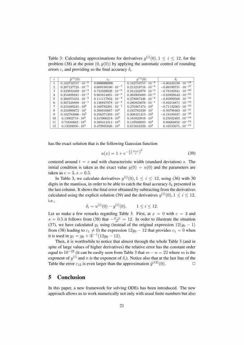
Table 3: Calculating approximations for derivatives y(i)(0), 1 ≤ i ≤ 12, for theproblem (38) at the point (0, y(0)) by applying the automatic control of roundingerrors εi and providing so the final accuracy δi

i y(i)(0) εi y(i)(0) δi1 0.182759757 · 10−6 0.0000000000 0.182759757 · 10−6 −0.60449198 · 10−28

2 0.207127725 · 10−5 0.609199190 · 10−7 0.213219716 · 10−5 −0.69190731 · 10−27

3 0.233932489 · 10−4 0.731039028 · 10−6 0.241242879 · 10−4 −0.78192941 · 10−26

4 0.254888941 · 10−3 0.901614801 · 10−5 0.263905089 · 10−3 −0.83928642 · 10−25

5 0.266975453 · 10−2 0.111117932 · 10−3 0.278087246 · 10−2 −0.85899500 · 10−24

6 0.267228880 · 10−1 0.136947978 · 10−2 0.280923676 · 10−1 −0.82216871 · 10−23

7 0.253489245 · 100 0.168782291 · 10−1 0.270367474 · 100 −0.71132365 · 10−22

8 0.224980672 · 101 0.208016667 · 100 0.245782339 · 101 −0.50790463 · 10−21

9 0.182784086 · 102 0.256371293 · 101 0.208421215 · 102 −0.19195037 · 10−20

10 0.13002719 · 103 0.315966218 · 102 0.161623816 · 103 0.25832403 · 10−19

11 0.71638662 · 103 0.389414314 · 103 0.110580093 · 104 0.86669850 · 10−18

12 0.13588050 · 104 0.479935826 · 104 0.615816329 · 104 0.16535675 · 10−16

has the exact solution that is the following Gaussian function

u(x) = 1 + e−12(

x−cs )

2

(39)

centered around t = c and with characteristic width (standard deviation) s. Theinitial condition is taken as the exact value y(0) = u(0) and the parameters aretaken as c = 3, s = 0.5.

In Table 3, we calculate derivatives y(i)(0), 1 ≤ i ≤ 12, using (36) with 30digits in the mantissa, in order to be able to catch the final accuracy δk presented inthe last column. It shows the final error obtained by subtracting from the derivativescalculated using the explicit solution (39) and the derivatives y(i)(0), 1 ≤ i ≤ 12,i.e.,

δi = u(i)(0)− y(i)(0), 1 ≤ i ≤ 12.

Let us make a few remarks regarding Table 3. First, at x = 0 with c = 3 ands = 0.5 it follows from (38) that −x−c

s2= 12. In order to illustrate the situation

(37), we have calculated y1 using (instead of the original expression 12(y0 − 1)from (38) leading to ε1 = 0) the expression 12y0 − 12 that provides ε1 = 0 whenit is used in y1 = y0 + ¬−1(12y0 − 12).

Then, it is worthwhile to notice that almost through the whole Table 3 (and inspite of large values of higher derivatives) the relative error has the constant orderequal to 10−22 (it can be easily seen from Table 3 that m− n = 22 where m is theexponent of y(i) and n is the exponent of δi). Notice also that at the last line of theTable the error ε12 is even larger than the approximation y(12)(0). 2

5 Conclusion

In this paper, a new framework for solving ODEs has been introduced. The newapproach allows us to work numerically not only with usual finite numbers but also

21

with different infinitesimal and infinite values on a new kind of a computationaldevice called the Infinity Computer (it has been patented and its working prototypeexists). The structure of numbers we work on the new computer is more complexand, as a result, we face new computational possibilities. In particular, the presenceof different numerical infinitesimals makes it possible to use infinitesimal steps forsolving ODEs. The following results have been established in the new framework.

i. It has been shown that (under the assumption that the person solving theODE does not know the structure of f(x, y), i.e., it is a “black box” for him/her)the Infinity Computer is able to calculate numerical values of the derivatives ofy(x) of the desired order without the necessity of an analytical (or symbolical)computation of the respective derivatives by the successive derivation of the ODEas it is usually done when the Taylor method is applied.

ii. If the region of our interest [a, b] belongs to the region of convergence of theTaylor expansion for the solution y(x) in the neighborhood of the point x0, then itis not necessary to construct iterative procedures involving several steps with finitevalues of h. It becomes possible to calculate approximations of the desired order kby executing k infinitesimal steps and only one finite step.

iii. Approximations of derivatives of y(x) at the point xn can be obtained usingthe information calculated at the point xn−1. For this purpose, instead of the usageof a finite step h, the steps h−¬−1 or h+¬−1 can be used. Methods going forwardand backward and working with approximations of derivatives can be proposed inthe new framework.

iv. The last subsection of the manuscript shows that either f(x, y) is evaluatedexactly or rounding errors are present, the Infinity Computer is able to perform, bymeans of a smart usage of infinitesimals, an automatic control of the accuracy ofcomputation of the derivatives of the solution.

v. Theoretical results have been illustrated by a number of numerical examples.

References

[1] R.A. Adams. Single variable calculus. Pearson Education Canada, Ontario,5 edition, 2003.

[2] V. Benci and M. Di Nasso. Numerosities of labeled sets: a new way ofcounting. Advances in Mathematics, 173:50–67, 2003.

[3] L. Brugnano and D. Trigiante. Solving Differential Problems by MultistepInitial and Boundary Value Methods. Gordon and Breach Science Publ., Am-sterdam, 1998.

[4] J. C. Butcher. Numerical methods for ordinary differential equations. JohnWiley & Sons, Chichester, 2 edition, 2003.

[5] G. Cantor. Contributions to the founding of the theory of transfinite numbers.Dover Publications, New York, 1955.

22

[6] J. R. Cash and S. Considine. An mebdf code for stiff initial value problems.ACM Trans. Math. Software, 18(2):142–155, 1992.

[7] J.H. Conway and R.K. Guy. The Book of Numbers. Springer-Verlag, NewYork, 1996.

[8] S. De Cosmis and R. De Leone. The use of grossone in mathematical pro-gramming and operations research. Applied Mathematics and Computation,218(16):8029–8038, 2012.

[9] L. D’Alotto. Cellular automata using infinite computations. Applied Mathe-matics and Computation, 218(16):8077–8082, 2012.

[10] B. Fornberg. Generation of finite difference formulas of arbitrarily spacedgrids. Mathematics of Computation, 51(184):699–706, 1988.

[11] P. Gordon. Numerical cognition without words: Evidence from Amazonia.Science, 306(15 October):496–499, 2004.

[12] A. Griewank and G.F. Corliss, editors. Automatic Differentiation of Al-gorithms: Theory, Implementation, and Application. SIAM, Philadelphia,Penn., 1991.

[13] E. Hairer, S. P. Nørsett, and G. Wanner. Solving ordinary differential equa-tions I: Nonstiff problems. Springer-Verlag, New York, 2 edition, 1993.

[14] P. Henrici. Applied and computational complex analysis, volume 1. JohnWiley & Sons, Chichester, 1997.

[15] F. Iavernaro and F. Mazzia. Solving ordinary differential equations by gen-eralized adams methods: properties and implementation techniques. Appl.Numer. Math., 28(2–4):107–126, 1998.

[16] D.I. Iudin, Ya.D. Sergeyev, and M. Hayakawa. Interpretation of percolationin terms of infinity computations. Applied Mathematics and Computation,218(16):8099–8111, 2012.

[17] J.D. Lambert. Numerical Methods for Ordinary Differential Systems: TheInitial Value Problem. John Wiley & Sons, Chichester, 1991.

[18] H.P. Langtangen and L. Wang. A Tutorial for the Odespy Interface toODE Solvers. http://hplgit.github.com/odespy/doc/tutorial/

html/wrap_odespy.html#using-adaptive-methods, 2012.

[19] G.W. Leibniz and J.M. Child. The Early Mathematical Manuscripts of Leib-niz. Dover Publications, New York, 2005.

[20] T. Levi-Civita. Sui numeri transfiniti. Rend. Acc. Lincei, Series 5a, 113:7–91,1898.

23

[21] G. Lolli. Infinitesimals and infinites in the history of mathematics: A briefsurvey. Applied Mathematics and Computation, 218(16):7979–7988, 2012.

[22] M. Margenstern. Using grossone to count the number of elements of infi-nite sets and the connection with bijections. p-Adic Numbers, UltrametricAnalysis and Applications, 3(3):196–204, 2011.

[23] M. Margenstern. An application of grossone to the study of a family oftilings of the hyperbolic plane. Applied Mathematics and Computation,218(16):8005–8018, 2012.

[24] J.M. Muller. Elementary functions: algorithms and implementation.Birkhauser, Boston, 2006.

[25] I. Newton. Method of Fluxions. 1671.

[26] P. Pica, C. Lemer, V. Izard, and S. Dehaene. Exact and approximate arithmeticin an amazonian indigene group. Science, 306(15 October):499–503, 2004.

[27] A.M. Quarteroni, R. Sacco, and F. Saleri. Numerical Mathematics. Springer-Verlag, New York, 2006.

[28] A. Robinson. Non-standard Analysis. Princeton Univ. Press, Princeton, 1996.

[29] E.E. Rosinger. Microscopes and telescopes for theoretical physics: How richlocally and large globally is the geometric straight line? Prespacetime Jour-nal, 2(4):601–624, 2011.

[30] Ya.D. Sergeyev. Arithmetic of Infinity. Edizioni Orizzonti Meridionali, CS,2003.

[31] Ya.D. Sergeyev. http://www.theinfinitycomputer.com. 2004.

[32] Ya.D. Sergeyev. Blinking fractals and their quantitative analysis using infiniteand infinitesimal numbers. Chaos, Solitons & Fractals, 33(1):50–75, 2007.

[33] Ya.D. Sergeyev. A new applied approach for executing computations withinfinite and infinitesimal quantities. Informatica, 19(4):567–596, 2008.

[34] Ya.D. Sergeyev. Evaluating the exact infinitesimal values of area of Sierpin-ski’s carpet and volume of Menger’s sponge. Chaos, Solitons & Fractals,42(5):3042–3046, 2009.

[35] Ya.D. Sergeyev. Numerical computations and mathematical modelling withinfinite and infinitesimal numbers. Journal of Applied Mathematics and Com-puting, 29:177–195, 2009.

24

[36] Ya.D. Sergeyev. Numerical point of view on Calculus for functions assum-ing finite, infinite, and infinitesimal values over finite, infinite, and infinitesi-mal domains. Nonlinear Analysis Series A: Theory, Methods & Applications,71(12):e1688–e1707, 2009.

[37] Ya.D. Sergeyev. Computer system for storing infinite, infinitesimal, and fini-te quantities and executing arithmetical operations with them. USA patent7,860,914, 2010.

[38] Ya.D. Sergeyev. Counting systems and the First Hilbert problem. Nonlin-ear Analysis Series A: Theory, Methods & Applications, 72(3-4):1701–1708,2010.

[39] Ya.D. Sergeyev. Lagrange Lecture: Methodology of numerical computa-tions with infinities and infinitesimals. Rendiconti del Seminario Matematicodell’Universita e del Politecnico di Torino, 68(2):95–113, 2010.

[40] Ya.D. Sergeyev. Higher order numerical differentiation on the infinity com-puter. Optimization Letters, 5(4):575–585, 2011.

[41] Ya.D. Sergeyev. On accuracy of mathematical languages used to deal withthe Riemann zeta function and the Dirichlet eta function. p-Adic Numbers,Ultrametric Analysis and Applications, 3(2):129–148, 2011.

[42] Ya.D. Sergeyev. Using blinking fractals for mathematical modelling of pro-cesses of growth in biological systems. Informatica, 22(4):559–576, 2011.

[43] Ya.D. Sergeyev and A. Garro. Observability of Turing machines: A refine-ment of the theory of computation. Informatica, 21(3):425–454, 2010.

[44] Ya.D. Sergeyev and A. Garro. Single-tape and multi-tape Turing machinesthrough the lens of the Grossone methodology. Journal of Supercomputing,2013, (to appear).

[45] M.C. Vita, S. De Bartolo, C. Fallico, and M. Veltri. Usage of infinitesimalsin the Menger’s Sponge model of porosity. Applied Mathematics and Com-putation, 218(16):8187–8196, 2012.

[46] J. Wallis. Arithmetica infinitorum. 1656.

[47] A.A. Zhigljavsky. Computing sums of conditionally convergent and divergentseries using the concept of grossone. Applied Mathematics and Computation,218(16):8064–8076, 2012.

[48] A. Zilinskas. On strong homogeneity of two global optimization algorithmsbased on statistical models of multimodal objective functions. Applied Math-ematics and Computation, 218(16):8131–8136, 2012.

25