Fuzzy Sets and Systems 161 (2010) 3064–3080www.elsevier.com/locate/fss

Solving multi-class problems with linguistic fuzzy rule basedclassification systems based on pairwise learning and

preference relations

Alberto Fernándeza,∗, María Calderónb, Edurne Barrenecheab,Humberto Bustinceb, Francisco Herrerac

a Department of Computer Science, University of Jaén, Spainb Department of Automatic and Computation, Public University of Navarra, Spain

c Department of Computer Science and Artificial Intelligence, CITIC-UGR (Research Center on Information and Communications Technology),University of Granada, Spain

Received 16 September 2009; received in revised form 10 May 2010; accepted 26 May 2010Available online 8 June 2010

Abstract

This paper deals with multi-class classification for linguistic fuzzy rule based classification systems. The idea is to decompose theoriginal data-set into binary classification problems using the pairwise learning approach (confronting all pair of classes), and toobtain an independent fuzzy system for each one of them. Along the inference process, each fuzzy rule based classification systemgenerates an association degree for both of its corresponding classes and these values are encoded into a fuzzy preference relation.

Our analysis is focused on the final step that returns the predicted class-label. Specifically, we propose to manage the fuzzypreference relation using a non-dominance criterion on the different alternatives, contrasting the behaviour of this model with boththe classical weighted voting scheme and a decision rule that combines the fuzzy relations of preference, conflict and ignorance bymeans of a voting strategy.

Our experimental study is carried out using two different linguistic fuzzy rule learning methods for which we show that the non-dominance criterion is a good alternative in comparison with the previously mentioned aggregation mechanisms. This empiricalanalysis is supported through the corresponding statistical analysis using non-parametrical tests.© 2010 Elsevier B.V. All rights reserved.

Keywords: Fuzzy rule-based classification systems; Multi-class problems; Fuzzy preference relations; Multi-classifiers; Pairwise learning

1. Introduction

Fuzzy rule based classification systems (FRBCSs) [27] are a popular tool among the computational intelligencetechniques employed to solve classification problems, because of their interpretable models based on linguisticvariables, which are easier to understand for the experts or end-users. They have been used in many real world

∗ Corresponding author. Tel.: +34953212444; fax: +34953212472.E-mail addresses: alberto.fernandez@ujaen.es (A. Fernández), Maria.CalderonTurullols@cajanavarra.es (M. Calderón),

edurne.barrenechea@unavarra.es (E. Barrenechea), bustince@unavarra.es (H. Bustince), herrera@decsai.ugr.es (F. Herrera).

0165-0114/$ - see front matter © 2010 Elsevier B.V. All rights reserved.doi:10.1016/j.fss.2010.05.016

A. Fernández et al. / Fuzzy Sets and Systems 161 (2010) 3064–3080 3065

classification problems such as medical applications [1], classification of battlefield ground vehicles [36] or intrusiondetection [30,34]. Some of these problems present a high number of classes, which must be considered in the FRBCSanalysis.

Multiclasses imply an additional difficulty for FRBCSs, since the boundaries among the classes can be overlapped,which causes a decrease of the performance. In this situation, we can proceed by transforming the original multi-class problem into binary subsets, which are easier to discriminate, via a class binarization technique [3,8]. In thispaper we study the extension of linguistic FRBCSs to a multi-classifier model considering the use of the pairwiselearning approach [20] (also called pairwise classification, round robin learning, all-pairs or one-vs-one), whichconsists in training a classifier for each possible pair of classes ignoring the examples that do not belong to the relatedclasses.

In order to aggregate the output for all binary classifiers, the simplest and most widely used method in pairwiselearning is applying a weighted voting [25] so that the final class is assigned by taking the maximum vote among thesummation of the scores for the binary classifiers associated to the same class. However, in this work we aim to benefitfrom the features of fuzzy classifiers and to make use of the framework of fuzzy preference relations for classification[23]. In this scheme, the classification problem is translated into a decision making problem for determining theoutput among all predictions for the binary classifiers. Specifically, in this paper we propose the use of a maximalnon-dominance criterion [31] for the final decision process.

In our study, we will first determine the goodness of the pairwise learning approach for linguistic fuzzy systemsanalysing the differences in performance achieved by a basic FRCBS model and the multi-classification approach.Furthermore, we will analyse the mentioned non-dominance criterion that we propose in contrast with both the standardweighted voting and a voting strategy introduced by Hühn and Hüllermeier in [22].

Our aim is to develop a complete empirical study in order to show that the non-dominance approach achieves avery good synergy with the linguistic fuzzy classifiers selected in this paper, namely the fuzzy hybrid genetics-basedmachine learning (FH-GBML) [29] and the structural learning algorithm in vague environment (SLAVE) [18,19]methods. We have taken 14 multi-class data-sets from UCI repository [4] within the experimental framework. Themeasure of performance is based on accuracy rate and the significance of results is supported by the proper statisticalanalysis as suggested in the literature [7,15].

To do so, this paper is organised as follows. In Section 2 we present the concept of multi-classification, a briefintroduction to linguistic FRBCS and the description of the fuzzy algorithm selected for our study. In Section 3 wepresent with detail the pairwise learning approach using fuzzy preference relations and the proposed methodologybased on a non-dominance criterion to carry out the classification step. Section 4 includes the experimental framework,that is, the description of the two aggregation schemes used for comparison in the experimental study, the benchmarkdata-sets, configuration parameters and the statistical tests for the performance comparison. In Section 5 we presentour empirical analysis. Finally, Section 6 concludes the paper. Additionally, we have included an Appendix with thecomplete tables of results for the experimental study.

2. Basic concepts on multi-classification and linguistic fuzzy rule based systems

This section first introduces the concept of multi-class problems and the class binarization technique selected forthis work. Then, we describe the main features of the linguistic FRBCSs. Finally, we describe the fuzzy rule learningapproaches used in this paper for the experimental study, the FH-GBML [29] and SLAVE [18] algorithms.

2.1. Multi-class problems via pairwise learning

There are a high amount of applications which require multi-class categorization. To simplify the classificationprocess, we can divide the initial problem into multiple two-class sets that can be solved separately. In this way, wetransform the problem boundaries by distinguishing only between two classes.

Specifically, we have considered the pairwise learning approach [20], which consists in training a classifier foreach possible pair of classes ignoring the examples that do not belong to the related classes. At classification time,a query instance is submitted to all binary models, and the predictions of these models are combined into an overallclassification.

3066 A. Fernández et al. / Fuzzy Sets and Systems 161 (2010) 3064–3080

The advantages of this approach with respect to other techniques, such as confronting one class with the rest (“one-vs-rest” [3]), are detailed below:

• It was shown to be more accurate for rule learning algorithms [11].• The computational time required for the learning phase is compensated by the reduction in size for each of the

individual problems.• The decision boundaries of each binary problem may be considerably simpler than the “one-vs-rest” transformation.• The selected binarization technique is less biased to obtain imbalanced training-sets [10,33], which may suppose an

added difficulty for the identification and discovery of rules covering the positive, and under-represented, samples.

2.2. Linguistic fuzzy rule based classification systems

Consider m labeled patterns x p = (x p1, . . . , x pn), p = 1, 2, . . . , m where x pi is the ith attribute value (i =1, 2, . . . , n). We have a set of linguistic values describing each attribute, considering the use of triangular membershipfunctions, in order to obtain fuzzy rules of the following form:

Rule j : If x1 is A j1 and . . . and xn is A jn then Class = C j with RW j (1)

where Rule j is the label of the jth rule, x = (x1, . . . , xn) is an n-dimensional pattern vector, A ji is an antecedent fuzzyset representing a linguistic term, C j is a class label, and RW j is the rule weight [26]. Specifically, we compute therule weight using the penalized certainty factor (PCF) defined in [28] as

PC Fj =∑

x p∈ClassC j�A j

(x p) − ∑x p /∈ClassC j

�A j(x p)∑m

p=1 �A j(x p)

(2)

Considering a new pattern x and being L the number of rules in the rule base (RB) and M the number of classes ofthe problem, the steps of the fuzzy reasoning method [5] are the following:

1. Matching degree. To calculate the strength of activation of the if-part for all rules in the RB with the pattern x p,using a product or minimum T-norm.

�A j(x p) = T (�A j1

(x p1), . . . , �A jn(x pn)), j = 1, . . . , L (3)

2. Association degree. To compute the association degree of the pattern x p with the M classes according to each rulein the RB. When using rules like (1) this association degree only refers to the consequent class of the rule:

bkj =

{h(�A j

(x p), RW j ), j = 1, . . . , L if k = Class(Rule j )0 otherwise

(4)

Function h is usually modeled as a product T-norm.3. Pattern classification soundness degree for all classes. We use an aggregation function f (for example the max

operator) that combines the positive degrees of association calculated in the previous step:

Yk = f (bkj , j = 1, . . . , L and bk

j > 0), k = 1, . . . , M (5)

4. Classification. We apply a decision function F over the soundness degree of the system for the pattern classificationfor all classes. This function will determine the class label l corresponding to the maximum value:

F(Y1, . . . , YM ) = arg maxk=1,. . .,M

{Yk} (6)

2.3. Linguistic fuzzy rule learning algorithms

Genetic fuzzy systems have been proposed in the specialized literature for designing fuzzy rule-based systemsby means of genetic algorithms (GAs) [6,21]. This type of search mechanisms have the ability to find near optimalsolutions in complex search spaces, which also have the advantage to provide a generic code structure and independentperformance features, making them suitable candidates to incorporate a priori knowledge. In the case of FRBCSs, this

A. Fernández et al. / Fuzzy Sets and Systems 161 (2010) 3064–3080 3067

a priori knowledge may be in the form of linguistic variables, fuzzy membership function parameters, fuzzy rules,number of rules, etc.

Taken into account the previous fact, we have selected two linguistic fuzzy rule learning based on genetic fuzzysystems, namely the FH-GBML [29] and the SLAVE [18] algorithms, which are described in the remainder of thissection. Both methods are available within the KEEL software tool [2] (http://www.keel.es).

2.3.1. Fuzzy hybrid genetics-based machine learning rule generation algorithmThe basis of the method described here, the FH-GBML algorithm [29], consists of a Pittsburgh approach where

each rule set is handled as an individual. It also contains a genetic cooperative competitive learning (GCCL) approach(an individual represents an unique rule), which is used as a kind of heuristic mutation for partially modifying eachrule set, because of its high search ability to efficiently find good fuzzy rules.

The system defines 14 possible linguistic terms for each attribute, as shown in Fig. 1, which correspond to Ruspini’sstrong fuzzy partitions with two, three, four, and five uniformly distributed triangular-shaped membership functions.Furthermore, the system also uses “don’t care” as an additional linguistic term, which indicates that the variable matchesany input value with maximum matching degree. We must point out that these fuzzy partitions are not modified duringthe evolutionary process.

The main steps of this algorithm are described below:Step 1: Generate Npop rule sets with Nrule fuzzy rules.Step 2: Calculate the fitness value of each rule set in the current population.Step 3: Generate (Npop −1) rule sets by selection, crossover and mutation in the same manner as the Pittsburgh-style

algorithm. Apply a single iteration of the GCCL-style algorithm (i.e., the rule generation and the replacement) to eachof the generated rule sets with a pre-specified probability.

Step 4: Add the best rule set in the current population to the newly generated (Npop − 1) rule sets to form the nextpopulation.

Step 5: Return to Step 2 if the pre-specified stopping condition is not satisfied.Next, we will describe every step of the algorithm:

• Initialization: Nrule training patterns are randomly selected. Then, a fuzzy rule from each of the selected trainingpatterns is generated by choosing probabilistically (as shown in (7)) an antecedent fuzzy set from the 14 candidatesBk (k = 1, 2, . . . , 14) (see Fig. 1) for each attribute. Then each antecedent fuzzy set of the generated fuzzy rule isreplaced with don’t care using a pre-specified probability Pdon′t care:

P(Bk) = �Bk(x pi )∑14

j=1 �B j(x pi )

(7)

0.0

0.0

0.0

0.0

0.0

0.0

0.0

0.0

1.0

1.0

1.0

1.0

1.0

1.0

1.0

1.0

Fig. 1. Four fuzzy partitions for each attribute membership function.

3068 A. Fernández et al. / Fuzzy Sets and Systems 161 (2010) 3064–3080

• Fitness computation: The fitness value of each rule set Si in the current population is calculated as the numberof correctly classified training patterns by Si . For the GCCL approach the computation follows the same scheme,counting the number of correct hits for each single rule.

• Selection: It is based on binary tournament in order to guarantee a good convergence of the population.• Crossover: The substring-wise and bit-wise uniform crossover are applied in the Pittsburgh part. In the case of the

GCCL part only the bit-wise uniform crossover is considered.• Mutation: Each fuzzy partition of the individuals is randomly replaced with a different fuzzy partition using a

pre-specified mutation probability for both approaches.

2.3.2. Structural learning algorithm in vague environmentSLAVE [18] is an iterative rule learning GA [35] which makes use of the disjunctive normal form for defining the

antecedent of the rules, using the formulation described in [17].The rule selection process consists in obtaining the best rule in each execution of the GA depending on the examples

of the training set. The concept of the best rule is based on the notions of consistency and completeness. The basicidea is to use the fuzzy cardinal of fuzzy sets “positive examples” and “negative examples” for a rule, which stands forthe combination of the match degrees of the rule for the examples of its consequent class and for the examples of theremaining classes.

The iterative approach of SLAVE fixes a class and the GA selects a rule that simultaneously verifies the completenessand the soft consistency condition to a high degree. The rule selection in SLAVE can therefore be solved by the followingoptimization problem:

maxA∈D

{�(RB(A)) × �k1,k2 (RB(A))} (8)

where D = P(D1) × P(D2) × · · · × P(Dn) with Di being the fuzzy domain of Xi variable, and RB(A) representsa rule with antecedent value A = (A1, . . . , An) ∈ D and consequent value B, with B being fixed in the optimizationproblem. �(RB(A)) and �k1,k2 (RB(A) represent the degree of completeness and the soft consistency degree of ruleRB(A), respectively (details can be found at [18]). The iterative approach will change this consequent value to obtainthe different values. Details of the GA used in this optimization process can be found in [16].

The implementation of the SLAVE considered in this paper considers the integration of a feature selection mech-anism, which was proposed in [19]. The most important change with respect to the original version of SLAVE is therepresentation of the population, which simply includes a new binary value associated to each antecedent variable inorder to discover if the variable will be considered as part of the antecedent of the rule or not.

3. Decision process for linguistic fuzzy rule based classification systems using preference relations formulti-class problems

In this section we will first describe in detail the learning scheme for a linguistic fuzzy system based on pairwiselearning. Then, we will introduce our proposal to carry out the final classification using a non-dominance criterion.

3.1. Pairwise learning approach for a linguistic fuzzy rule based classification system

Following the pairwise learning approach, we start dividing the original training set into m(m − 1)/2 subsets, wherem stands for the number of classes of the problem, in order to obtain m(m − 1)/2 different fuzzy classifiers. Everysubset contains the examples for a different pair of classes and thus, the trained classifiers are devoted to discriminatebetween two specific classes of the initial data-set.

The knowledge base (KB) of each one of these fuzzy classifiers will be composed of a shared data base (DB) and aspecific RB. We decided to obtain such an interpretable model rather than just contextualizing the fuzzy partitions foreach sub-problem separately, with the aim of being able to analyse the different rule sets learnt by means of the binaryclassifiers in a uniform manner.

The RB for each classifier is learnt using a fuzzy learning method, which can be selected among the differentapproaches of the specialized literature. Once all KBs have been learnt, we proceed to the final inference step. When

A. Fernández et al. / Fuzzy Sets and Systems 161 (2010) 3064–3080 3069

a new input pattern is presented to the system, each FRBCS is fired in order to define the output degree for its pair ofassociated classes.

3.2. On the use of fuzzy preference relations for classification

In this subsection we describe how we compute the fuzzy preference relation with the use of the output degrees ofthe different FRBCSs that compose the system. Then, we detail the classification step using a maximal non-dominancecriterion.

3.2.1. Computation of the fuzzy preference relationWe will consider the classification problem as a decision making problem, and we will define a fuzzy preference

relation Rb [31] with the corresponding outputs of the FRBCSs. In this manner, the computation of each degree ofpreference is based on the aggregation function that combines the positive degrees of association between the fuzzyrules and the input pattern. This is known as fuzzy reasoning method:

Rb =

⎡⎢⎢⎢⎣

− r1,2 . . . r1,m

r2,1 − . . . r2,m...

. . .. . .

...

rm,1 rm,1 . . . −

⎤⎥⎥⎥⎦ (9)

We consider the maximum matching, where every new pattern x p is classified as the consequent class of a singlewinner rule (Class(x p) = Cw) which is determined as

�Aw(x p) · RWw = max{�Aq

(x p) · RWq , Ruleq ∈ RB} (10)

where �Aq(x p) is the membership degree of the pattern example x p = (x p1, . . . , x pn) with the antecedent of the rule

Rq and RWq is the rule weight [26].Therefore, Rb(i, j) (the fuzzy degree of preference between classes i and j) is the maximum association degree for

all rules in RB that concludes class i. Rb(i, j) will be normalized to [0, 1] by expression (11), having the relationR(i, j) = 1 − R( j, i):

R(i, j) = Rb(i, j)

Rb(i, j) + Rb( j, i)(11)

In the possible case that Rb(i, j) and Rb( j, i) are equal to 0, because no rule for the binary classifier matches theexample, we set R(i, j) and R( j, i) a 0.5 value so that the fuzzy preference relation remains reciprocal.

3.2.2. Classification process via a decision rule based on a non-dominance criterionFrom the fuzzy preference relation we must extract a set of non-dominated alternatives (classes) as the solution

of the fuzzy decision making problem and thus, our classification output. Specifically, the maximal non-dominatedelements of R are calculated by means of the following operations, according to the non-dominance criterion proposedby Orlovsky [31]:

• First, we compute the fuzzy strict preference relation R′ which is equal to

R′(i, j) ={

R(i, j) − R( j, i) when R(i, j) > R( j, i)0 otherwise

(12)

• Then, we compute the non-dominance degree of each class N Di , which is simply obtained as

N Di = 1 − supj∈C

[R′( j, i)] (13)

3070 A. Fernández et al. / Fuzzy Sets and Systems 161 (2010) 3064–3080

This value represents the degree to which the class i is dominated by no one of the remaining classes. C stands for theset of total classes in the data-set. The output class is computed as the index of the maximal non-dominance value:

Class(x p) = arg maxi=1,. . .,m

{N Di } (14)

The complete process is summarized in Algorithm 1

Algorithm 1. Procedure for the multi-classifier learning proposal with the non-dominance criterion

1. Divide the training set into m(m − 1)/2 subsets for all pair of classes.2. For each training subset i:

2.1. Build a fuzzy classifier composed by a local DB and an RB generated with any rule learning procedure3. For each input test pattern:

3.1. Build a fuzzy preference relation R as:• For each class i, i = 1, . . . , m• For each class j, j = 1, . . . , m, j � i• The preference degree for R(i, j) is the normalized association degree for the classifier associated to classes i and j. R( j, i) = 1 − R(i, j)

3.2 Transform R to the fuzzy strict preference relation R′.3.3 Compute the degree of non-dominance for all classes.3.4 The input pattern is assigned to the class with maximum non-dominance value.

In order to clarify this procedure, we use a pattern from the iris data-set (Table 1) to show an example which isdepicted in Table 2. We also show, for the sake of determining the global interpretability of the output model, the wholeRB obtained by the FH-GBML algorithm for this current example in Table 3.

Table 1Iris data-set pattern.

Sepal length=7.0,Sepal width=3.2,Petal length=4.7,Petal width=1.4,

Class=Versicolor{Setosa, Versicolor, Virginica}

Table 2Example of the classification process by means of the use of the fuzzy preference relation with the non-dominance criterion.

Step 1. Obtain Rb:

Rb =

⎡⎢⎣ − 0.134 0.221

0.881 − 0.1170.625 0.021 −

⎤⎥⎦

Step 2. Normalize Rb → R:

R =

⎡⎢⎣ − 0.132 0.261

0.868 − 0.8480.738 0.152 −

⎤⎥⎦

Step 3. Transform R to R′:

R′ =

⎡⎢⎣

− 0.0 0.00.736 − 0.6960.477 0.0 −

⎤⎥⎦

Step 4. Compute ND:ND = {0.264, 1.0, 0.304}

Step 5. Get class index:Class = arg max

i=1,. . .,3{N Di } = 2 (V ersicolor )

A. Fernández et al. / Fuzzy Sets and Systems 161 (2010) 3064–3080 3071

Table 3Example: rule base obtained by FH-GBML for the Iris data-set.

Rule base for Setosa vs. Versicolor (20 rules):

1: IF SL IS L0(2) AND SW IS L0(3) AND PL IS L1(2) AND PW IS L1(2): Versicolor with RW: 0.993742: IF SW IS L1(3): Setosa with RW: 0.048483: IF SW IS L0(2) AND PW IS L0(2): Setosa with RW: 0.080154: IF PL IS L2(4): Versicolor with RW: 1.05: IF SW IS L1(2) AND PL IS L0(2) AND PW IS L0(2): Setosa with RW: 0.769676: IF PL IS L0(2): Setosa with RW: 0.359337: IF PL IS L2(4) AND PW IS L2(4): Versicolor with RW: 1.08: IF SL IS L1(3) AND PW IS L2(4): Versicolor with RW: 1.09: IF SL IS L2(4) AND PL IS L2(4): Versicolor with RW: 1.010: IF SW IS L0(2): Versicolor with RW: 0.2379111: IF SL IS L0(2) AND SW IS L1(3) AND PW IS L0(4): Setosa with RW: 1.012: IF SL IS L2(5) AND PW IS L2(4): Versicolor with RW: 1.013: IF SL IS L1(3): Versicolor with RW: 0.3277914: IF SL IS L1(3) AND SW IS L0(2) AND PL IS L0(2): Versicolor with RW: 0.2794915: IF SL IS L0(2) AND PL IS L1(4) AND PW IS L1(3): Versicolor with RW: 0.7380716: IF SL IS L1(5) AND PL IS L1(3): Versicolor with RW: 0.3260817: IF SL IS L1(3) AND PW IS L0(2): Versicolor with RW: 0.0080618: IF SL IS L1(4) AND SW IS L1(2): Setosa with RW: 0.3922419: IF SL IS L0(4) AND SW IS L2(4) AND PL IS L0(3): Setosa with RW: 1.020: IF SW IS L1(3) AND PW IS L0(3): Setosa with RW: 0.93428

Rule base for Setosa vs. Virginica (19 rules):

1: IF SL IS L1(5) AND PL IS L0(3) AND PW IS L1(3): Setosa with RW: 1.02: IF SL IS L1(5): Setosa with RW: 0.833333: IF SL IS L1(4): Setosa with RW: 0.396424: IF PW IS L2(4): Virginica with RW: 1.05: IF SL IS L0(3) AND SW IS L1(3) AND PW IS L0(4): Setosa with RW: 1.06: IF SL IS L1(5) AND PW IS L0(5): Setosa with RW: 1.07: IF SL IS L1(4) AND SW IS L2(4): Setosa with RW: 0.792888: IF PW IS L0(3): Setosa with RW: 1.09: IF SL IS L2(4) AND SW IS L2(5) AND PW IS L1(2): Virginica with RW: 1.010: IF SL IS L0(4) AND SW IS L2(4) AND PW IS L0(5): Setosa with RW: 1.011: IF SL IS L0(2) AND PL IS L4(5): Virginica with RW: 1.012: IF SL IS L0(2) AND SW IS L1(4) AND PL IS L2(4): Virginica with RW: 1.013: IF PL IS L1(5) AND PW IS L0(2): Setosa with RW: 1.014: IF SW IS L1(3): Virginica with RW: 0.0294515: IF PL IS L0(2): Setosa with RW: 0.5934216: IF SW IS L1(3): Virginica with RW: 0.0294517: IF SL IS L1(5) AND SW IS L2(5) AND PL IS L0(2) AND PW IS L0(2): Setosa with RW: 0.9929018: IF PL IS L0(3): Setosa with RW: 1.019: IF SW IS L1(4) AND PL IS L1(3): Virginica with RW: 0.75813

Rule base for Versicolor vs. Virginica (14 rules):

1: IF SW IS L2(5) AND PL IS L0(2) AND PW IS L3(5): Virginica with RW: 0.285472: IF SL IS L2(5) AND PL IS L3(4) AND PW IS L2(4): Virginica with RW: 0.906163: IF SL IS L2(5) AND SW IS L1(3) AND PL IS L2(3): Virginica with RW: 0.438964: IF SW IS L2(4) AND PL IS L2(4) AND PW IS L3(5): Virginica with RW: 0.284345: IF SL IS L0(2) AND PL IS L1(3) AND PW IS L2(3): Virginica with RW: 0.590156: IF SL IS L3(5) AND SW IS L0(3) AND PL IS L3(4) AND PW IS L3(5): Virginica with RW: 0.990837: IF SL IS L2(4) AND SW IS L0(3) AND PL IS L0(2): Versicolor with RW: 0.269598: IF SL IS L3(5) AND PL IS L2(4) AND PW IS L0(2): Versicolor with RW: 0.288699: IF SL IS L0(3) AND SW IS L2(4) AND PL IS L3(5) AND PW IS L0(3): Versicolor with RW: 1.010: IF SL IS L3(5) AND SW IS L2(3) AND PL IS L3(5) AND PW IS L1(4): Versicolor with RW: 1.011: IF SL IS L1(2) AND SW IS L1(3) AND PL IS L1(4) AND PW IS L2(4): Versicolor with RW: 0.9092912: IF SL IS L0(2) AND SW IS L1(3) AND PL IS L2(4) AND PW IS L1(3): Versicolor with RW: 0.3866213: IF SL IS L3(4) AND SW IS L0(4) AND PL IS L1(3) AND PW IS L1(3): Versicolor with RW: 0.3957714: IF SL IS L2(3) AND SW IS L2(3) AND PL IS L1(3) AND PW IS L1(2): Virginica with RW: 0.86992

3072 A. Fernández et al. / Fuzzy Sets and Systems 161 (2010) 3064–3080

4. Experimental framework

In this section, we will first introduce the two aggregation schemes used for comparison with our non-dominancecriterion (Section 4.1). Then, we will provide details of the real-world multi-class problems chosen for the experimen-tation and the configuration parameters of the FRBCSs (Sections 4.2 and 4.3, respectively). Finally, we will introducethe statistical tests applied to compare the results obtained along the experimental study (Section 4.4).

4.1. Mechanisms for combining predictions in pairwise classification used for comparison

In this part of the section we introduce two classification process for combining the predictions in the pairwiselearning scheme that we have selected for contrasting the behaviour of the non-dominance criterion, namely a weightedvoting scheme and a decision rule based on a voting strategy.

4.1.1. Classification process via a weighted voting schemeThe first technique is one of the simplest and most widely used aggregation method in pairwise learning [25]. The

final class is assigned by computing the maximum vote by rows from the values of the fuzzy preference relation R:

Class(x p) = arg maxi=1,. . .,m

{∑mj=1; j�i R(i, j)

m − 1

}(15)

We must point out that in this case R is a normalised reciprocal matrix which means that whenever a binary classifieris not able to determine the association degree for a given instance, it outputs a 0.5 value for both classes. In spite ofits simplicity, it has been determined to obtain a very good precision for pairwise classification [24,25].

4.1.2. Classification process via a decision rule based on a voting strategyThis voting strategy was proposed in [22] and starts from the obtention of Rb(i, j) and Rb( j, i) as the maximum

association output degrees for the rule set for classes i and j and compute R as the normalised version of Rb. Wemust point out that in spite of in the original proposal of this voting strategy the values of R(i, j) and R( j, i) arenon-normalised, in this paper we have taken a normalised reciprocal matrix (as in the weighted voting scheme) sinceit provides better results in practice with the fuzzy algorithms selected in our experimental framework. From here, thefollowing values are derived:

P(i, j) = R(i, j) − min{R(i, j), R( j, i)}P( j, i) = R( j, i) − min{R(i, j), R( j, i)}C(i, j) = min{R(i, j), R( j, i)}I (i, j) = 1 − max{R(i, j), R( j, i)} (16)

C(i, j) is defined as the degree of conflict, namely the degree to which both classes are supported. Likewise, I (i, j)is the degree of ignorance, namely the degree to which none of the classes is supported. Finally, P(i, j) and P( j, i)denote the strict preference for i and j, respectively. Note that at least one of these two degrees is zero, and thatP(i, j) + P( j, i) + C(i, j) + I (i, j) = 1.

From these three relations, the following classification rule could be used:

Class(x p) = arg maxi=1,. . .,m

∑1≤ j � i≤m

P(i, j) + 1

2· C(i, j) + Ni

Ni + N j· I (i, j) (17)

where Ni is the number of examples from class i in the training data (and hence, an unbiased estimate of the classprobability).

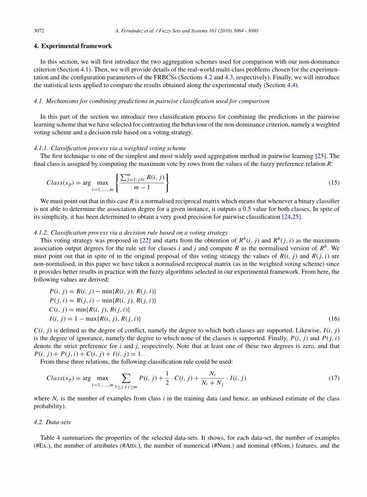
4.2. Data-sets

Table 4 summarizes the properties of the selected data-sets. It shows, for each data-set, the number of examples(#Ex.), the number of attributes (#Atts.), the number of numerical (#Num.) and nominal (#Nom.) features, and the

A. Fernández et al. / Fuzzy Sets and Systems 161 (2010) 3064–3080 3073

Table 4Summary description of the data-sets.

id Data-set #Ex. #Atts. #Num. #Nom. #Cl.

bal balance scale 625 4 4 0 3cle cleveland 297 13 6 7 5eco ecoli 336 7 7 0 8gla glass identification 214 9 9 0 6iri iris 150 4 4 0 3let letter 2000 16 16 0 26new new-thyroid 215 5 5 0 3pag page-blocks 548 10 10 0 5pen pen-based 1099 16 16 0 10

recognitionseg segment 2310 19 19 0 7shu shuttle 2175 9 9 0 5veh vehicle 846 18 18 0 4win wine 178 13 13 0 3yea yeast 1484 8 8 0 10

number of classes (#Cl.). The letter, penbased and page-blocks data-sets have been stratified sampled at 10% in orderto reduce their size for training. In the case of missing values (cleveland) we have removed those instances from thedata-set.

Estimates of accuracy rate were obtained by means of a fivefold cross-validation. That is, we split the data set intofive folds, each one containing the 20% of the patterns of the data-set. For each fold, the algorithm was trained withthe examples contained in the remaining folds and then, tested with the current fold. Furthermore, we have run thealgorithms three times in order to obtain a sample of 15 results, which have been averaged, for each data-set.

4.3. Parameters

The selected configuration for the FH-GBML and SLAVE approaches has been set up according to the recommen-dations of the authors in the corresponding papers. Regarding the specific parameters for the genetic process, we havechosen the following values:

• FH-GBML:◦ Number of fuzzy rules: 5 · d rules.◦ Number of rule sets: 200 rule sets.◦ Crossover probability: 0.9.◦ Mutation probability: 1/d .◦ Number of replaced rules: All rules except the best-one (Pittsburgh-part, elitist approach), number of rules/5

(GCCL-part).◦ Total number of generations: 1000 generations.◦ Don’t care probability: 0.5.◦ Probability of the application of the GCCL iteration: 0.5.

• SLAVE:◦ Population size: 100 individuals.◦ Number of iterations allowed without change=500 iterations.◦ Mutation probability=0.01.◦ Crossover probability=1.0 (it is always applied)

where d stands for the dimensionality of the problem (number of variables). Whereas the mutation probability isoriginally taken from the recommendations given in Ishibuchi and Yamamoto’s paper [29], the number of rules hasbeen chosen heuristically after some preliminary experiments in order to obtain a good behaviour for all data-sets, alsofollowing the same scheme than in some of our previous works using this algorithm [9].

3074 A. Fernández et al. / Fuzzy Sets and Systems 161 (2010) 3064–3080

4.4. Statistical tests for performance comparison

In this paper, we use the hypothesis testing techniques to provide statistical support to the analysis of the results[13,32]. Specifically, we will use non-parametric tests, due to the fact that the initial conditions that guarantee thereliability of the parametric tests may not be satisfied, making the statistical analysis to lose credibility with these typeof tests [7].

We apply the Wilcoxon signed-rank test [32] as non-parametric statistical procedure for performing pairwise com-parisons between two algorithms. We will also compute the p-value associated to each comparison, which representsthe lowest level of significance of a hypothesis that results in a rejection. In this manner, we can know whether twoalgorithms are significantly different and how different they are.

Furthermore, we consider the average ranking of the algorithms in order to show graphically how good a methodis with respect to its partners. This ranking is obtained by assigning a position to each algorithm depending on itsperformance for each data-set. The algorithm which achieves the best accuracy on a specific data-set will have the firstranking (value 1); then, the algorithm with the second best accuracy is assigned rank 2, and so forth. This task is carriedout for all data-sets and finally an average ranking is computed as the mean value of all rankings.

These tests are suggested in the studies presented in [7,13–15], where its use in the field of machine learning ishighly recommended. Any interested reader can find additional information on the Website http://sci2s.ugr.es/sicidm/,together with the software for applying the statistical tests.

5. Experimental analysis

The results of the experiments in the test partitions for the FH-GBML and SLAVE algorithms are shown in Tables 5and 6 where, by columns, we can observe the accuracy performance for the basic algorithm and the pairwise-learningapproaches, namely the non-dominance classification criterion (noted with suffix ND), the weighted voting scheme(noted with suffix WV) and the decision rule based on a voting strategy (noted with suffix VS). The complete tables ofresults with the training and test partitions are shown in the appendix of this paper.

We divide our experimental analysis into two parts:

• First, we want to determine whether the multi-classifier proposal enhances the performance of the linguistic FRBCSthat manages all classes independently.

• Next, our aim is to analyse the behaviour of our proposal for the output decision process based on a non-dominancecriterion versus the weighted voting and the voting strategy.

Table 5Average accuracy results for the FH-GBML algorithm with the basic approach and the multi-classifier schemes.

Data-set #Cl. FH-GBML FH-GBML-ND FH-GBML-WV FH-GBML-VS

Bal 3 82.24 ± 2.85 84.80 ± 2.83 84.32 ± 2.86 84.96 ± 2.55Iri 3 93.33 ± 4.08 94.67 ± 2.98 94.00 ± 2.79 94.00 ± 2.79New 3 91.16 ± 3.03 95.35 ± 2.33 94.42 ± 2.65 94.42 ± 1.27Win 3 92.70 ± 4.21 96.08 ± 3.75 94.38 ± 3.96 93.83 ± 4.58Veh 4 58.15 ± 3.47 66.67 ± 4.37 66.20 ± 3.81 66.08 ± 4.57Cle 5 50.84 ± 6.14 57.24 ± 2.45 57.58 ± 2.33 57.92 ± 1.96Pag 5 94.53 ± 0.91 95.62 ± 1.20 95.62 ± 1.77 95.62 ± 1.77Shu 5 95.22 ± 1.43 97.70 ± 0.83 97.79 ± 1.33 95.40 ± 2.16Gla 6 60.29 ± 6.30 62.19 ± 7.58 64.04 ± 8.84 63.59 ± 6.90Seg 7 78.70 ± 2.27 93.29 ± 1.73 89.26 ± 2.41 89.26 ± 2.41Eco 8 76.19 ± 5.04 81.55 ± 4.63 79.77 ± 3.04 76.80 ± 6.48Pen 10 69.82 ± 1.84 91.09 ± 1.14 92.18 ± 1.97 92.18 ± 1.97Yea 10 51.22 ± 4.54 58.96 ± 1.53 58.42 ± 2.41 57.21 ± 2.00Let 26 16.35 ± 1.58 71.20 ± 2.35 72.75 ± 1.88 72.55 ± 2.02

Mean X 72.20 ± 3.41 81.89 ± 2.84 81.48 ± 3.00 80.99 ± 3.10

A. Fernández et al. / Fuzzy Sets and Systems 161 (2010) 3064–3080 3075

Table 6Average accuracy results for the SLAVE algorithm with the basic approach and the multi-classifier schemes.

Data-set #Cl. SLAVE SLAVE-ND SLAVE-WV SLAVE-VS

Bal 3 77.76 ± 2.07 75.20 ± 4.12 75.36 ± 3.85 75.36 ± 3.85Iri 3 96.00 ± 3.65 96.67 ± 2.36 97.33 ± 2.79 97.33 ± 2.79New 3 90.70 ± 2.85 91.16 ± 6.02 90.23 ± 6.02 80.93 ± 3.03Win 3 93.78 ± 3.77 96.05 ± 3.24 88.71 ± 9.52 87.05 ± 7.33Veh 64.07 ± 2.17 60.87 ± 5.59 58.03 ± 3.89 58.03 ± 3.34Cle 5 52.84 ± 6.25 54.92 ± 5.40 55.24 ± 3.67 56.59 ± 4.30Pag 5 93.61 ± 1.74 93.61 ± 1.96 93.42 ± 1.53 93.24 ± 1.42Shu 5 85.70 ± 0.50 94.76 ± 2.91 91.77 ± 1.24 90.76 ± 1.02Gla 6 61.20 ± 3.78 56.07 ± 3.88 54.65 ± 5.07 52.79 ± 6.76Seg 7 89.26 ± 1.27 90.04 ± 1.32 75.24 ± 3.53 75.24 ± 3.53Eco 8 85.41 ± 6.29 79.46 ± 6.04 77.09 ± 4.89 77.38 ± 2.88Pen 10 88.73 ± 2.44 89.18 ± 2.17 59.36 ± 4.33 59.73 ± 3.86Yea 10 50.74 ± 4.28 56.13 ± 1.56 50.41 ± 2.29 49.40 ± 1.96Let 26 41.85 ± 2.11 68.80 ± 2.39 51.00 ± 1.96 51.05 ± 2.15

Mean X 76.55 ± 3.08 78.78 ± 3.50 72.70 ± 3.90 71.78 ± 3.44

2.29

4.00

1.931.79

0.00

0.50

1.00

1.50

2.00

2.50

3.00

3.50

4.00

4.50

Basic ND WV VS

Fig. 2. Ranking in accuracy for the different FH-GBML approaches: basic scheme, multi-classifier with non-dominance criterion and multi-classifierwith voting strategy.

5.1. Analysis on the usefulness of the pairwise learning approach for linguistic fuzzy rule based classification systems

In order to carry out the first study, we show the ranking of the FH-GBML and SLAVE approaches by means of theprocedure described in Section 4.4. Figs. 2 and 3 show the average ranking computed for the four different alternatives:basic approach and the three multi-classification techniques. We can observe that for the FH-GBML algorithm all themulti-classification schemes obtain a higher average result and ranking than the basic methodology, whereas in thecase of the SLAVE algorithm only the non-dominance criterion is competitive with the basic approach.

In order to determine with a statistical support that the non-dominance criterion outperforms the basic linguisticFRBCS approach, we will carry out a Wilcoxon test for both algorithms (FH-GBML and SLAVE), which is shown inTable 7. The result of this test is in concordance with our previous hypothesis for which the multiclassifier version ofthe FRBCSs derives in a benefit in performance.

5.2. Analysis of the decision process methodology

The next objective of this empirical analysis is to study the three alternatives selected for the decision process amongall predictions for the fuzzy classifiers. With this aim, we have carried out a Wilcoxon test, shown in Table 8, in whichwe compare the non-dominance criterion versus the weighted voting and the voting strategy.

3076 A. Fernández et al. / Fuzzy Sets and Systems 161 (2010) 3064–3080

3.04

1.75

2.96

2.25

0.00

0.50

1.00

1.50

2.00

2.50

3.00

3.50

Basic ND WV VS

Fig. 3. Ranking in accuracy for the different SLAVE approaches: basic scheme, multi-classifier with non-dominance criterion and multi-classifierwith voting strategy.

Table 7Wilcoxon test to compare the multiclassifier FBRCS (non-dominance approach) versus the basic approach for the FH-GBML and SLAVE algorithms.

Comparison R+ R− p-value Hypothesis (� = 0.05)

FH-GBML-ND vs. FH-GBML 105.0 0.0 0.001 Rejected for FH-GBML-NDSLAVE-ND vs. SLAVE 65.5 39.5 0.463 Not rejected

R+ corresponds to the sum of the ranks for the multiclassifier approach and R− to the basic approach.

Table 8Wilcoxon test to compare the non-dominance approach versus the weighted voting and the decision rule with a voting strategy for the FH-GBMLand SLAVE algorithms.

Comparison R+ R− p-Value Hypothesis (� = 0.05)

FH-GBML-ND vs. FH-GBML-WV 67.5 37.5 0.345 Not rejectedFH-GBML-ND vs. FH-GBML-VS 73.5 31.5 0.173 Not rejected

SLAVE-ND vs. SLAVE-WV 97.0 8.0 0.005 Rejected for SLAVE-NDSLAVE-ND vs. SLAVE-VS 97.0 8.0 0.005 Rejected for SLAVE-ND

R+ corresponds to the sum of the ranks for the non-dominance criterion and R− to the weighted voting (first and third row) and the voting strategy(second and fourth row).

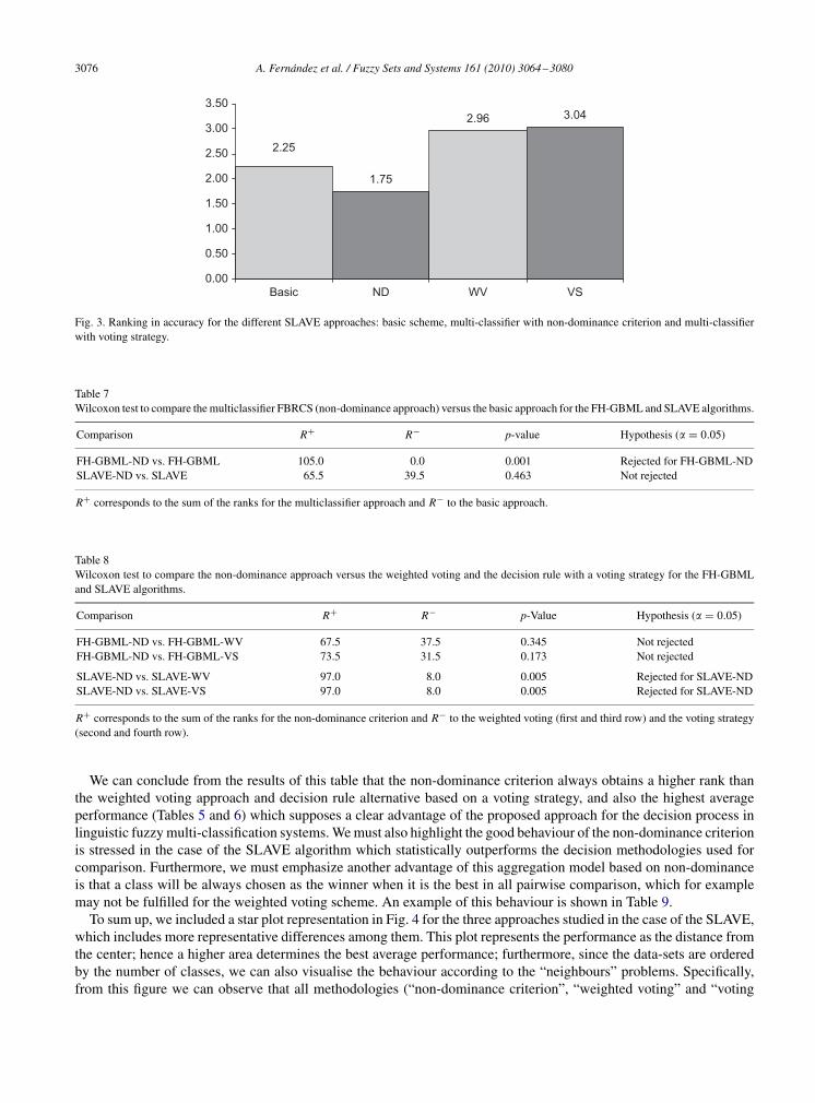
We can conclude from the results of this table that the non-dominance criterion always obtains a higher rank thanthe weighted voting approach and decision rule alternative based on a voting strategy, and also the highest averageperformance (Tables 5 and 6) which supposes a clear advantage of the proposed approach for the decision process inlinguistic fuzzy multi-classification systems. We must also highlight the good behaviour of the non-dominance criterionis stressed in the case of the SLAVE algorithm which statistically outperforms the decision methodologies used forcomparison. Furthermore, we must emphasize another advantage of this aggregation model based on non-dominanceis that a class will be always chosen as the winner when it is the best in all pairwise comparison, which for examplemay not be fulfilled for the weighted voting scheme. An example of this behaviour is shown in Table 9.

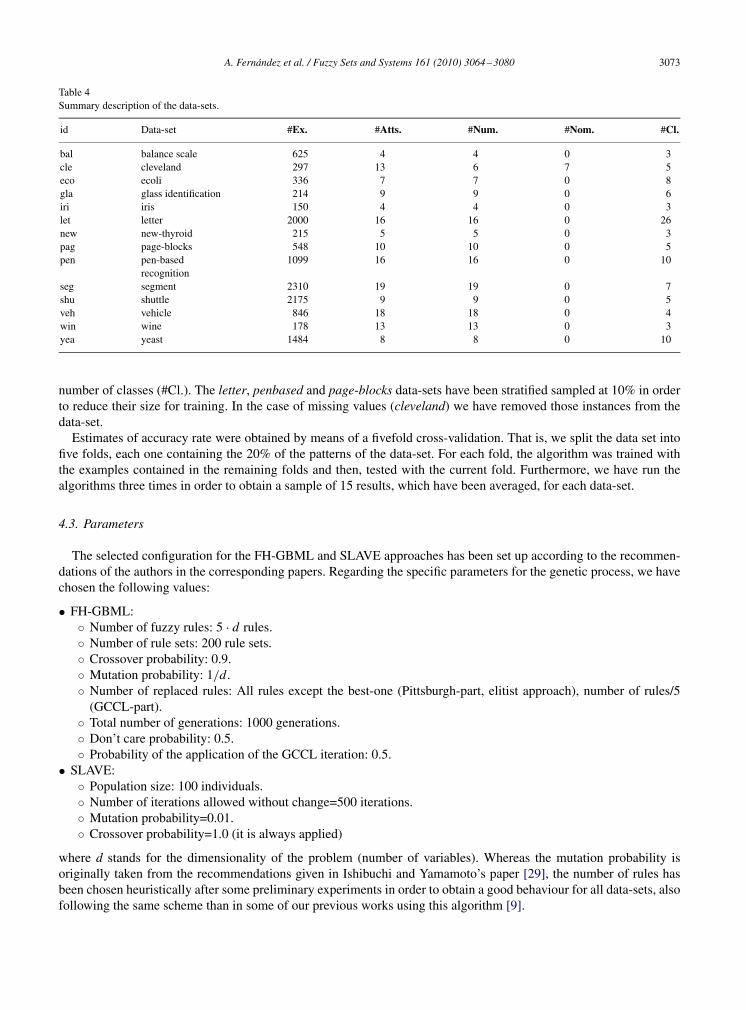
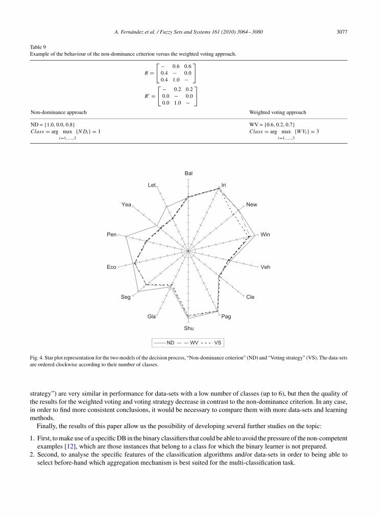
To sum up, we included a star plot representation in Fig. 4 for the three approaches studied in the case of the SLAVE,which includes more representative differences among them. This plot represents the performance as the distance fromthe center; hence a higher area determines the best average performance; furthermore, since the data-sets are orderedby the number of classes, we can also visualise the behaviour according to the “neighbours” problems. Specifically,from this figure we can observe that all methodologies (“non-dominance criterion”, “weighted voting” and “voting

A. Fernández et al. / Fuzzy Sets and Systems 161 (2010) 3064–3080 3077

Table 9Example of the behaviour of the non-dominance criterion versus the weighted voting approach.

R =⎡⎣ − 0.6 0.6

0.4 − 0.00.4 1.0 −

⎤⎦

R′ =⎡⎣ − 0.2 0.2

0.0 − 0.00.0 1.0 −

⎤⎦

Non-dominance approach Weighted voting approach

ND = {1.0, 0.0, 0.8} WV = {0.6, 0.2, 0.7}Class = arg max

i=1,. . .,3{N Di } = 1 Class = arg max

i=1,. . .,3{W Vi } = 3

Bal

Iri

New

Win

Veh

Cle

Pag

Shu

Gla

Seg

Eco

Pen

Yea

Let

ND WV VS

Fig. 4. Star plot representation for the two models of the decision process, “Non-dominance criterion” (ND) and “Voting strategy” (VS). The data-setsare ordered clockwise according to their number of classes.

strategy”) are very similar in performance for data-sets with a low number of classes (up to 6), but then the quality ofthe results for the weighted voting and voting strategy decrease in contrast to the non-dominance criterion. In any case,in order to find more consistent conclusions, it would be necessary to compare them with more data-sets and learningmethods.

Finally, the results of this paper allow us the possibility of developing several further studies on the topic:

1. First, to make use of a specific DB in the binary classifiers that could be able to avoid the pressure of the non-competentexamples [12], which are those instances that belong to a class for which the binary learner is not prepared.

2. Second, to analyse the specific features of the classification algorithms and/or data-sets in order to being able toselect before-hand which aggregation mechanism is best suited for the multi-classification task.

3078 A. Fernández et al. / Fuzzy Sets and Systems 161 (2010) 3064–3080

3. Related to the previous issue, we are interested in proposing a kind of theoretical argument or explanation for whythe “non-dominance criterion” is better than “weighted voting” and in which cases.

4. Finally, to study a way to unify the potential of the aggregation schemes compared in this paper so that, regardingthe previous items, we could obtain an approach that shows a good synergy for different frameworks.

6. Concluding remarks

In this paper, we have applied a pairwise learning methodology for building a linguistic fuzzy multi-classifier systemoriented to discriminate between pairs of classes and to obtain a better decision boundary in multiclass problems.

In order to aggregate the output for every single classifier, we have made use of a fuzzy preference relation translatingthe classification problem into a decision making problem. For obtaining the final output class, we have proposed theuse of a decision rule based on a maximal non-dominance criterion, and we have contrasted the behaviour of thismodel with the classical weighted voting method and a new voting strategy based on the fuzzy relations of preference,ignorance and conflict.

The experimental study showed two main conclusions: First, the application of a pairwise learning approach usingthe non-dominance criterion improves the performance of the linguistic FRBCS methods. Second, we have foundempirical evidences in favour of the non-dominance criterion for the final classification, being the best alternative inthis context, especially when the number of classes of the problem is high.

Finally, we have pointed out some interesting issues as future work so that this paper can be taken as a starting pointfor carrying out several new studies on the topic.

Acknowledgment

This work had been supported by the Spanish Ministry of Science and Technology under Projects TIN2008-06681-C06-01 and TIN2007-65981.

Appendix: Complete tables of results

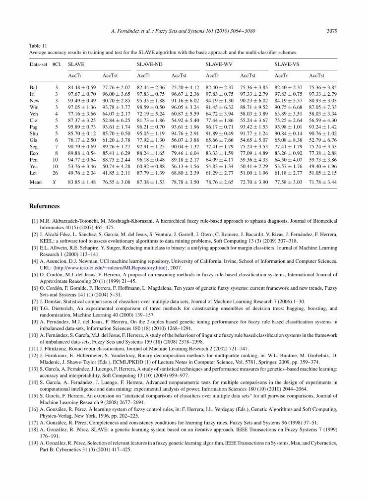
The complete tables of results for the experimental study are shown in Tables 10 and 11.

Table 10Average accuracy results in training and test for the FH-GBML algorithm with the basic approach and the multi-classifier schemes.

Data-set #Cl. FH-GBML FH-GBML-ND FH-GBML-WV FH-GBML-VS

AccTr AccTst AccTr AccTst AccTr AccTst AccTr AccTst

Bal 3 85.64 ± 2.49 82.24 ± 2.85 87.04 ± 1.97 84.80 ± 2.83 87.16 ± 1.91 84.32 ± 2.86 86.96 ± 1.95 84.96 ± 2.55Iri 3 99.33 ± 0.70 93.33 ± 4.08 99.50 ± 0.46 94.67 ± 2.98 98.17 ± 1.09 94.00 ± 2.79 98.17 ± 1.09 94.00 ± 2.79New 3 96.74 ± 0.66 91.16 ± 3.03 99.53 ± 0.49 95.35 ± 2.33 96.05 ± 1.26 94.42 ± 2.65 93.72 ± 1.26 94.42 ± 1.27Win 3 97.61 ± 0.63 92.70 ± 4.21 100.00 ± 0.00 96.08 ± 3.75 98.74 ± 0.92 94.38 ± 3.96 98.31 ± 1.46 93.83 ± 4.58Veh 4 62.44 ± 1.07 58.15 ± 3.47 74.50 ± 1.11 66.67 ± 4.37 73.82 ± 0.91 66.20 ± 3.81 73.79 ± 0.78 66.08 ± 4.57Cle 5 63.05 ± 0.73 50.84 ± 6.14 75.59 ± 0.82 57.24 ± 2.45 75.93 ± 1.06 57.58 ± 2.33 74.07 ± 0.62 57.92 ± 1.96Pag 5 95.67 ± 0.51 94.53 ± 0.91 98.17 ± 0.49 95.62 ± 1.20 97.08 ± 0.93 95.62 ± 1.77 96.49 ± 0.94 95.62 ± 1.77Shu 5 95.52 ± 0.67 95.22 ± 1.43 98.45 ± 0.60 97.70 ± 0.83 98.34 ± 0.43 97.79 ± 1.33 95.54 ± 1.44 95.40 ± 2.16Gla 6 70.44 ± 0.37 60.29 ± 6.30 82.48 ± 0.72 62.19 ± 7.58 74.88 ± 1.13 64.04 ± 8.84 73.83 ± 1.48 63.59 ± 6.90Seg 7 79.82 ± 1.19 78.70 ± 2.27 94.96 ± 0.35 93.29 ± 1.73 90.78 ± 2.17 89.26 ± 2.41 90.78 ± 2.17 89.26 ± 2.41Eco 8 79.76 ± 1.44 76.19 ± 5.04 92.34 ± 1.27 81.55 ± 4.63 88.39 ± 1.62 79.77 ± 3.04 84.75 ± 1.02 76.80 ± 6.48Pen 10 71.93 ± 1.19 69.82 ± 1.84 96.41 ± 0.63 91.09 ± 1.14 96.84 ± 0.33 92.18 ± 1.97 96.82 ± 0.35 92.18 ± 1.97Yea 10 53.84 ± 1.26 51.22 ± 4.54 65.47 ± 0.70 58.96 ± 1.53 62.35 ± 0.38 58.42 ± 2.41 61.19 ± 0.51 57.21 ± 2.00Let 26 18.19 ± 1.64 16.35 ± 1.58 86.30 ± 0.31 71.20 ± 2.35 84.65 ± 0.93 72.75 ± 1.88 84.58 ± 1.02 72.55 ± 2.02

Mean X 76.43 ± 1.04 72.20 ± 3.41 89.34 ± 0.71 81.89 ± 2.84 87.37 ± 1.08 81.48 ± 3.00 86.36 ± 1.15 80.99 ± 3.10

A. Fernández et al. / Fuzzy Sets and Systems 161 (2010) 3064–3080 3079

Table 11Average accuracy results in training and test for the SLAVE algorithm with the basic approach and the multi-classifier schemes.

Data-set #Cl. SLAVE SLAVE-ND SLAVE-WV SLAVE-VS

AccTr AccTst AccTr AccTst AccTr AccTst AccTr AccTst

Bal 3 84.48 ± 0.59 77.76 ± 2.07 82.44 ± 2.36 75.20 ± 4.12 82.40 ± 2.37 75.36 ± 3.85 82.40 ± 2.37 75.36 ± 3.85Iri 3 97.67 ± 0.70 96.00 ± 3.65 97.83 ± 0.75 96.67 ± 2.36 97.83 ± 0.75 97.33 ± 2.79 97.83 ± 0.75 97.33 ± 2.79New 3 93.49 ± 0.49 90.70 ± 2.85 95.35 ± 1.88 91.16 ± 6.02 94.19 ± 1.30 90.23 ± 6.02 84.19 ± 5.57 80.93 ± 3.03Win 3 97.05 ± 1.36 93.78 ± 3.77 98.59 ± 0.50 96.05 ± 3.24 91.45 ± 6.32 88.71 ± 9.52 90.75 ± 6.68 87.05 ± 7.33Veh 4 77.16 ± 3.66 64.07 ± 2.17 72.19 ± 5.24 60.87 ± 5.59 64.72 ± 3.94 58.03 ± 3.89 63.89 ± 3.51 58.03 ± 3.34Cle 5 87.37 ± 3.25 52.84 ± 6.25 81.73 ± 1.86 54.92 ± 5.40 77.44 ± 1.86 55.24 ± 3.67 75.25 ± 2.64 56.59 ± 4.30Pag 5 95.89 ± 0.73 93.61 ± 1.74 96.21 ± 0.70 93.61 ± 1.96 96.17 ± 0.71 93.42 ± 1.53 95.98 ± 1.01 93.24 ± 1.42Shu 5 85.70 ± 0.12 85.70 ± 0.50 95.05 ± 1.19 94.76 ± 2.91 91.89 ± 0.49 91.77 ± 1.24 90.84 ± 0.14 90.76 ± 1.02Gla 6 76.17 ± 2.50 61.20 ± 3.78 77.92 ± 1.30 56.07 ± 3.88 65.66 ± 7.66 54.65 ± 5.07 65.08 ± 8.38 52.79 ± 6.76Seg 7 90.79 ± 0.69 89.26 ± 1.27 92.91 ± 1.25 90.04 ± 1.32 77.41 ± 1.79 75.24 ± 3.53 77.41 ± 1.79 75.24 ± 3.53Eco 8 89.88 ± 0.54 85.41 ± 6.29 88.24 ± 1.65 79.46 ± 6.04 83.33 ± 1.59 77.09 ± 4.89 83.26 ± 0.92 77.38 ± 2.88Pen 10 94.77 ± 0.64 88.73 ± 2.44 96.18 ± 0.48 89.18 ± 2.17 64.09 ± 4.17 59.36 ± 4.33 64.50 ± 4.07 59.73 ± 3.86Yea 10 53.76 ± 3.46 50.74 ± 4.28 60.92 ± 0.88 56.13 ± 1.56 54.83 ± 1.34 50.41 ± 2.29 53.57 ± 1.76 49.40 ± 1.96Let 26 49.76 ± 2.04 41.85 ± 2.11 87.79 ± 1.39 68.80 ± 2.39 61.29 ± 2.77 51.00 ± 1.96 61.18 ± 2.77 51.05 ± 2.15

Mean X 83.85 ± 1.48 76.55 ± 3.08 87.38 ± 1.53 78.78 ± 3.50 78.76 ± 2.65 72.70 ± 3.90 77.58 ± 3.03 71.78 ± 3.44

References

[1] M.R. Akbarzadeh-Totonchi, M. Moshtagh-Khorasani, A hierarchical fuzzy rule-based approach to aphasia diagnosis, Journal of BiomedicalInformatics 40 (5) (2007) 465–475.

[2] J. Alcalá-Fdez, L. Sánchez, S. García, M. del Jesus, S. Ventura, J. Garrell, J. Otero, C. Romero, J. Bacardit, V. Rivas, J. Fernández, F. Herrera,KEEL: a software tool to assess evolutionary algorithms to data mining problems, Soft Computing 13 (3) (2009) 307–318.

[3] E.L. Allwein, R.E. Schapire, Y. Singer, Reducing multiclass to binary: a unifying approach for margin classifiers, Journal of Machine LearningResearch 1 (2000) 113–141.

[4] A. Asuncion, D.J. Newman, UCI machine learning repository, University of California, Irvine, School of Information and Computer Sciences.URL: 〈http://www.ics.uci.edu/∼mlearn/MLRepository.html〉, 2007.

[5] O. Cordón, M.J. del Jesus, F. Herrera, A proposal on reasoning methods in fuzzy rule-based classification systems, International Journal ofApproximate Reasoning 20 (1) (1999) 21–45.

[6] O. Cordón, F. Gomide, F. Herrera, F. Hoffmann, L. Magdalena, Ten years of genetic fuzzy systems: current framework and new trends, FuzzySets and Systems 141 (1) (2004) 5–31.

[7] J. Demšar, Statistical comparisons of classifiers over multiple data sets, Journal of Machine Learning Research 7 (2006) 1–30.[8] T.G. Dietterich, An experimental comparison of three methods for constructing ensembles of decision trees: bagging, boosting, and

randomization, Machine Learning 40 (2000) 139–157.[9] A. Fernández, M.J. del Jesus, F. Herrera, On the 2-tuples based genetic tuning performance for fuzzy rule based classification systems in

imbalanced data-sets, Information Sciences 180 (18) (2010) 1268–1291.[10] A. Fernández, S. García, M.J. del Jesus, F. Herrera, A study of the behaviour of linguistic fuzzy rule based classification systems in the framework

of imbalanced data-sets, Fuzzy Sets and Systems 159 (18) (2008) 2378–2398.[11] J. Fürnkranz, Round robin classification, Journal of Machine Learning Research 2 (2002) 721–747.[12] J. Fürnkranz, E. Hüllermeier, S. Vanderlooy, Binary decomposition methods for multipartite ranking, in: W.L. Buntine, M. Grobelnik, D.

Mladenic, J. Shawe-Taylor (Eds.), ECML/PKDD (1) of Lecture Notes in Computer Science, Vol. 5781, Springer, 2009, pp. 359–374.[13] S. García, A. Fernández, J. Luengo, F. Herrera, A study of statistical techniques and performance measures for genetics–based machine learning:

accuracy and interpretability, Soft Computing 13 (10) (2009) 959–977.[14] S. García, A. Fernández, J. Luengo, F. Herrera, Advanced nonparametric tests for multiple comparisons in the design of experiments in

computational intelligence and data mining: experimental analysis of power, Information Sciences 180 (10) (2010) 2044–2064.[15] S. García, F. Herrera, An extension on “statistical comparisons of classifiers over multiple data sets” for all pairwise comparisons, Journal of

Machine Learning Research 9 (2008) 2677–2694.[16] A. González, R. Pérez, A learning system of fuzzy control rules, in: F. Herrera, J.L. Verdegay (Eds.), Genetic Algorithms and Soft Computing,

Physica-Verlag, New York, 1996, pp. 202–225.[17] A. González, R. Pérez, Completeness and consistency conditions for learning fuzzy rules, Fuzzy Sets and Systems 96 (1998) 37–51.[18] A. González, R. Pérez, SLAVE: a genetic learning system based on an iterative approach, IEEE Transactions on Fuzzy Systems 7 (1999)

176–191.[19] A. González, R. Pérez, Selection of relevant features in a fuzzy genetic learning algorithm, IEEE Transactions on Systems, Man, and Cybernetics,

Part B: Cybernetics 31 (3) (2001) 417–425.

3080 A. Fernández et al. / Fuzzy Sets and Systems 161 (2010) 3064–3080

[20] T. Hastie, R. Tibshirani, Classification by pairwise coupling, The Annals of Statistics 26 (2) (1998) 451–471.[21] F. Herrera, Genetic fuzzy systems: taxonomy, current research trends and prospects, Evolutionary Intelligence 1 (2008) 27–46.[22] J.C. Hühn, E. Hüllermeier, FR3: a fuzzy rule learner for inducing reliable classifiers, IEEE Transactions on Fuzzy Systems 17 (1) (2009)

138–149.[23] E. Hüllermeier, K. Brinker, Learning valued preference structures for solving classification problems, Fuzzy Sets and Systems 159 (18) (2008)

2337–2352.[24] E. Hüllermeier, J. Fürnkranz, Comparison of ranking procedures in pairwise preference learning. In: Proceedings of the 10th International

Conference on Information Processing and Management of Uncertainty in Knowledge-Based Systems IPMU04, Vol. 11, 2004.[25] E. Hüllermeier, S. Vanderlooy, Combining predictions in pairwise classification: an optimal adaptive voting strategy and its relation to weighted

voting, Pattern Recognition 43 (1) (2010) 128–142.[26] H. Ishibuchi, T. Nakashima, Effect of rule weights in fuzzy rule-based classification systems, IEEE Transactions on Fuzzy Systems 9 (4) (2001)

506–515.[27] H. Ishibuchi, T. Nakashima, M. Nii, Classification and Modeling with Linguistic Information Granules: Advanced Approaches to Linguistic

Data Mining, Springer-Verlag, 2004.[28] H. Ishibuchi, T. Yamamoto, Rule weight specification in fuzzy rule-based classification systems, IEEE Transactions on Fuzzy Systems 13

(2005) 428–435.[29] H. Ishibuchi, T. Yamamoto, T. Nakashima, Hybridization of fuzzy GBML approaches for pattern classification problems, IEEE Transactions

on System, Man and Cybernetics B 35 (2) (2005) 359–365.[30] J. Marín-Blázquez, G.M. Pérez, Intrusion detection using a linguistic hedged fuzzy-XCS classifier system, Soft Computing 13 (3) (2009)

273–290.[31] S. Orlovsky, Decision-making with a fuzzy preference relation, Fuzzy Sets and Systems 1 (1978) 155–167.[32] D. Sheskin, Handbook of Parametric and Nonparametric Statistical Procedures, second ed., Chapman & Hall/CRC, 2006.[33] Y. Sun, A.C. Wong, M.S. Kamel, Classification of imbalanced data: a review, International Journal of Pattern Recognition and Artificial

Intelligence 23 (4) (2009) 687–719.[34] C. Tsang, S. Kwong, H. Wang, Genetic-fuzzy rule mining approach and evaluation of feature selection techniques for anomaly intrusion

detection, Pattern Recognition 40 (9) (2007) 2373–2391.[35] G. Venturini, SIA: a supervised inductive algorithm with genetic search for learning attributes based concepts, in: P. Brazdil (Ed.), Machine

Learning ECML—93 of Lecture Notes in Artificial Intelligence, Vol. 667, Springer, 1993, pp. 280–296.[36] H. Wu, J. Mendel, Classification of battlefield ground vehicles using acoustic features and fuzzy logic rule-based classifiers, IEEE Transactions

on Fuzzy Systems 15 (1) (2007) 56–72.