Solving Linear Recurrence Equations With

Polynomial Coefficients

Marko PetkovsekFaculty of Mathematics and Physics

University of LjubljanaJadranska 19, SI-1000 Ljubljana, Slovenia

marko.petkovsek@fmf.uni-lj.si

Helena ZakrajsekFaculty of Mechanical Engineering

University of LjubljanaAskerceva 6, SI-1000 Ljubljana, Slovenia

helena.zakrajsek@fs.uni-lj.si

Abstract

Summation is closely related to solving linear recurrence equations,since an indefinite sum satisfies a first-order linear recurrence with con-stant coefficients, and a definite proper-hypergeometric sum satisfies alinear recurrence with polynomial coefficients. Conversely, d’Alembertiansolutions of linear recurrences can be expressed as nested indefinite sumswith hypergeometric summands. We sketch the simplest algorithms forfinding polynomial, rational, hypergeometric, d’Alembertian, and Liou-villian solutions of linear recurrences with polynomial coefficients, andrefer to the relevant literature for state-of-the-art algorithms for thesetasks. We outline an algorithm for finding the minimal annihilatorof a given P-recursive sequence, prove the salient closure properties ofd’Alembertian sequences, and present an alternative proof of a recentresult of Reutenauer’s that Liouvillian sequences are precisely the inter-lacings of d’Alembertian ones.

1 Introduction

Summation is related to solving linear recurrence equations in several ways. Anindefinite sum

s(n) =

n−1∑k=0

t(k)

1

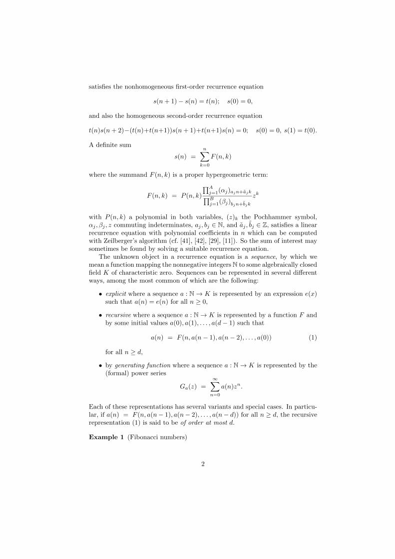
satisfies the nonhomogeneous first-order recurrence equation

s(n+ 1)− s(n) = t(n); s(0) = 0,

and also the homogeneous second-order recurrence equation

t(n)s(n+ 2)−(t(n)+t(n+1))s(n+ 1)+t(n+1)s(n) = 0; s(0) = 0, s(1) = t(0).

A definite sum

s(n) =

n∑k=0

F (n, k)

where the summand F (n, k) is a proper hypergeometric term:

F (n, k) = P (n, k)

∏Aj=1(αj)ajn+ajk∏Bj=1(βj)bjn+bjk

zk

with P (n, k) a polynomial in both variables, (z)k the Pochhammer symbol,αj , βj , z commuting indeterminates, aj , bj ∈ N, and aj , bj ∈ Z, satisfies a linearrecurrence equation with polynomial coefficients in n which can be computedwith Zeilberger’s algorithm (cf. [41], [42], [29], [11]). So the sum of interest maysometimes be found by solving a suitable recurrence equation.

The unknown object in a recurrence equation is a sequence, by which wemean a function mapping the nonnegative integers N to some algebraically closedfield K of characteristic zero. Sequences can be represented in several differentways, among the most common of which are the following:

• explicit where a sequence a : N→ K is represented by an expression e(x)such that a(n) = e(n) for all n ≥ 0,

• recursive where a sequence a : N→ K is represented by a function F andby some initial values a(0), a(1), . . . , a(d− 1) such that

a(n) = F (n, a(n− 1), a(n− 2), . . . , a(0)) (1)

for all n ≥ d,

• by generating function where a sequence a : N→ K is represented by the(formal) power series

Ga(z) =

∞∑n=0

a(n)zn.

Each of these representations has several variants and special cases. In particu-lar, if a(n) = F (n, a(n− 1), a(n− 2), . . . , a(n− d)) for all n ≥ d, the recursiverepresentation (1) is said to be of order at most d.

Example 1 (Fibonacci numbers)

2

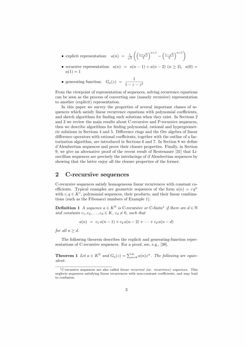
• explicit representation: a(n) = 1√5

((1+√5

2

)n+1

−(

1−√5

2

)n+1)

• recursive representation: a(n) = a(n − 1) + a(n − 2) (n ≥ 2), a(0) =a(1) = 1

• generating function: Ga(z) =1

1− z − z2

From the viewpoint of representation of sequences, solving recurrence equationscan be seen as the process of converting one (namely recursive) representationto another (explicit) representation.

In this paper we survey the properties of several important classes of se-quences which satisfy linear recurrence equations with polynomial coefficients,and sketch algorithms for finding such solutions when they exist. In Sections 2and 3 we review the main results about C-recursive and P-recursive sequences,then we describe algorithms for finding polynomial, rational and hypergeomet-ric solutions in Sections 4 and 5. Difference rings and the Ore algebra of lineardifference operators with rational coefficients, together with the outline of a fac-torization algorithm, are introduced in Sections 6 and 7. In Section 8 we defined’Alembertian sequences and prove their closure properties. Finally, in Section9, we give an alternative proof of the recent result of Reutenauer [31] that Li-ouvillian sequences are precisely the interlacings of d’Alembertian sequences byshowing that the latter enjoy all the closure properties of the former.

2 C-recursive sequences

C-recursive sequences satisfy homogeneous linear recurrences with constant co-efficients. Typical examples are geometric sequences of the form a(n) = c qn

with c, q ∈ K∗, polynomial sequences, their products, and their linear combina-tions (such as the Fibonacci numbers of Example 1).

Definition 1 A sequence a ∈ KN is C-recursive or C-finite1 if there are d ∈ Nand constants c1, c2, . . . , cd ∈ K, cd 6= 0, such that

a(n) = c1 a(n− 1) + c2 a(n− 2) + · · ·+ cd a(n− d)

for all n ≥ d.

The following theorem describes the explicit and generating-function repre-sentations of C-recursive sequences. For a proof, see, e.g., [38].

Theorem 1 Let a ∈ KN and Ga(z) =∑∞n=0 a(n)zn. The following are equiv-

alent:

1C-recursive sequences are also called linear recurrent (or: recurrence) sequences. Thisneglects sequences satisfying linear recurrences with non-constant coefficients, and may leadto confusion.

3

1. a is C-recursive,

2. a(n) =

r∑i=1

Pi(n)αni for all n ∈ N where Pi ∈ K[x] and αi ∈ K,

3. Ga(z) =P (z)

Q(z)where P,Q ∈ K[x], degP < degQ and Q(0) 6= 0.

The next two theorems are easy corollaries of Theorem 1.

Theorem 2 The set of C-recursive sequences is closed under the following bi-nary operations (a, b) 7→ c:

1. addition: c(n) = a(n) + b(n)

2. (Hadamard or termwise) multiplication: c(n) = a(n)b(n)

3. convolution (Cauchy multiplication): c(n) =∑ni=0 a(i)b(n− i)

4. interlacing: 〈c(0), c(1), c(2), c(3), . . .〉 = 〈a(0), b(0), a(1), b(1), . . .〉

Remark 1 These operations extend naturally to any nonzero number ofoperands.

Theorem 3 The set of C-recursive sequences is closed under the followingunary operations a 7→ c:

1. scalar multiplication: c(n) = λa(n) (λ ∈ K)

2. (left) shift: c(n) = a(n+ 1)

3. indefinite summation: c(n) =∑nk=0 a(k)

4. multisection: c(n) = a(mn+ r) (m, r ∈ N, 0 ≤ r < m)

That (nonzero) C-recursive sequences are not closed under taking reciprocalsis demonstrated, e.g., by a(n) = n+ 1 which is C-recursive while its reciprocalb(n) = 1/(n + 1) is not, since its generating function Gb(x) = − ln(1 − x)/xis not a rational function. Of course, there are C-recursive sequences whosereciprocals are C-recursive as well, such as all the geometric sequences.

Question 1. When are a and 1/a both C-recursive?

Theorem 4 The sequences a and 1/a are both C-recursive iff a is the interlac-ing of one or more geometric sequences.

For a proof, see [26].

4

3 P-recursive sequences

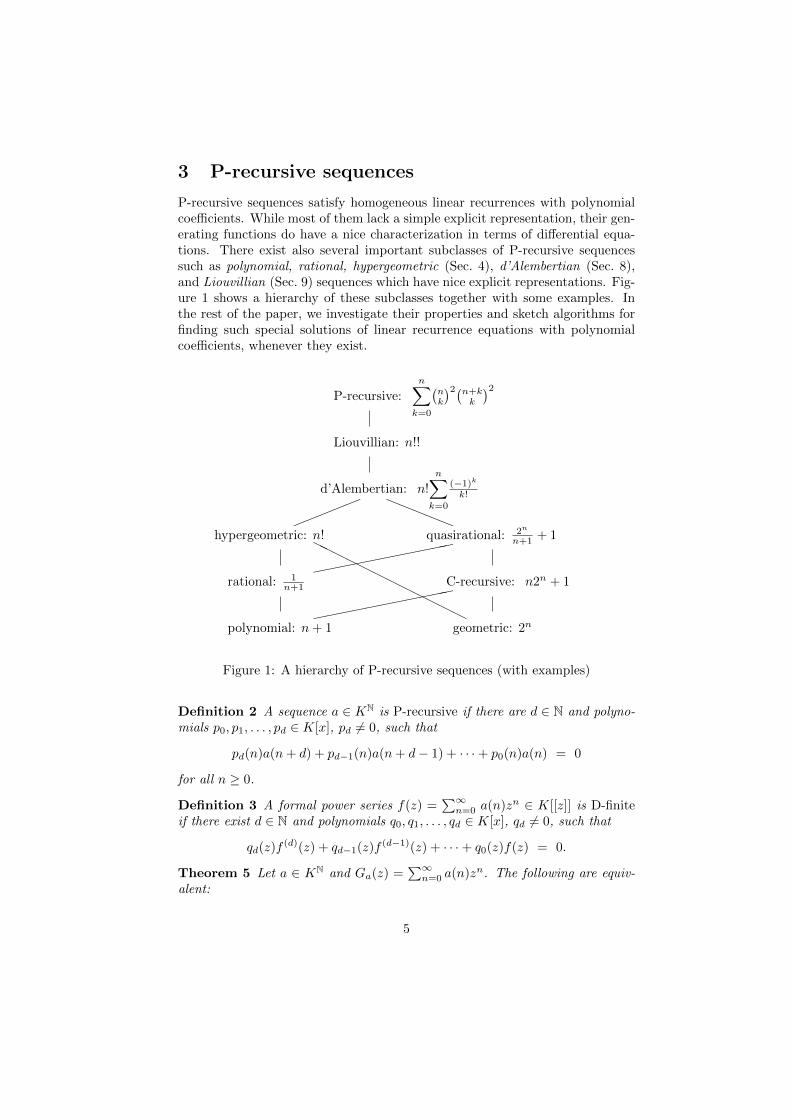
P-recursive sequences satisfy homogeneous linear recurrences with polynomialcoefficients. While most of them lack a simple explicit representation, their gen-erating functions do have a nice characterization in terms of differential equa-tions. There exist also several important subclasses of P-recursive sequencessuch as polynomial, rational, hypergeometric (Sec. 4), d’Alembertian (Sec. 8),and Liouvillian (Sec. 9) sequences which have nice explicit representations. Fig-ure 1 shows a hierarchy of these subclasses together with some examples. Inthe rest of the paper, we investigate their properties and sketch algorithms forfinding such special solutions of linear recurrence equations with polynomialcoefficients, whenever they exist.

polynomial: n+ 1 geometric: 2n

rational: 1n+1 C-recursive: n2n + 1

hypergeometric: n! quasirational: 2n

n+1 + 1

d’Alembertian: n!

n∑k=0

(−1)kk!

Liouvillian: n!!

P-recursive:

n∑k=0

(nk

)2(n+kk

)2

HHH

HHH

HHH

HHH

!!!!

!

aaaa

a

Figure 1: A hierarchy of P-recursive sequences (with examples)

Definition 2 A sequence a ∈ KN is P-recursive if there are d ∈ N and polyno-mials p0, p1, . . . , pd ∈ K[x], pd 6= 0, such that

pd(n)a(n+ d) + pd−1(n)a(n+ d− 1) + · · ·+ p0(n)a(n) = 0

for all n ≥ 0.

Definition 3 A formal power series f(z) =∑∞n=0 a(n)zn ∈ K[[z]] is D-finite

if there exist d ∈ N and polynomials q0, q1, . . . , qd ∈ K[x], qd 6= 0, such that

qd(z)f(d)(z) + qd−1(z)f (d−1)(z) + · · ·+ q0(z)f(z) = 0.

Theorem 5 Let a ∈ KN and Ga(z) =∑∞n=0 a(n)zn. The following are equiv-

alent:

5

1. a is P-recursive,

2. Ga(z) is D-finite.

For a proof, see [39] or [40].

Theorem 6 P-recursive sequences are closed under the following operations:

1. addition,

2. multiplication,

3. convolution,

4. interlacing,

5. scalar multiplication,

6. shift,

7. indefinite summation,

8. multisection.

For a proof, see [40].

Question 2. When are a and 1/a are both P-recursive?

The answer is given in Theorem 7.

Example 2 The sequences a(n) = n! and b(n) = 1/n! are both P-recursivesince a(n+ 1)− (n+ 1)a(n) = 0 and (n+ 1)b(n+ 1)− b(n) = 0.

Example 3 The sequence a(n) = 2n+1 is P-recursive (even C-recursive) whileits reciprocal b(n) = 1/(2n + 1) is not P-recursive.

Proof: We use the fact that a D-finite function can have at most finitely manysingularities in the complex plane (see, e.g., [40]). The generating function

Gb(z) =

∞∑n=0

b(n)zn =

∞∑n=0

zn

2n + 1

obviously has radius of convergence equal to two. We can rewrite

Gb(2z) =

∞∑n=0

2n

2n + 1zn =

∞∑n=0

(1− 1

2n + 1

)zn

=1

1− z−Gb(z). (2)

At z = 1 the function 1/(1 − z) is singular, Gb is regular, so Gb is singular atz = 2. At z = 2 the function 1/(1−z) is regular, Gb is singular, so Gb is singularat z = 4. At z = 4 the function 1/(1 − z) is regular, Gb is singular, so Gb issingular at z = 8, and so on. By induction on k it follows that Gb(z) is singularat z = 2k for all k ∈ N, k ≥ 1, hence Gb is not D-finite, and b is not P-recursive.�

6

4 Hypergeometric sequences

Hypergeometric sequences are P-recursive sequences which satisfy homogeneouslinear recurrence equations with polynomial coefficients of order one. Theycan be represented explicitly as products of rational functions, Pochhammersymbols, and geometric sequences. The algorithm for finding hypergeomet-ric solutions of linear recurrence equations with polynomial coefficients playsan important role in other, more involved computational tasks such as findingd’Alembertian or Liouvillian solutions, and factoring linear recurrence opera-tors.

Definition 4 A sequence a ∈ KN is hypergeometric2 if there is an N ∈ N suchthat a(n) 6= 0 for all n ≥ N , and there are polynomials p, q ∈ K[n] \ {0} suchthat

p(n) a(n+ 1) = q(n) a(n) (3)

for all n ≥ 0. We denote by H(K) the set of all hypergeometric sequences inKN.

Clearly, each hypergeometric sequence is P-recursive.

Proposition 1 The set H(K) is closed under the following operations:

1. multiplication,

2. reciprocation,

3. nonzero scalar multiplication,

4. shift,

5. multisection.

Proof: For 1 – 4, see [29]. For multisection, let a ∈ H(K) satisfy (3) and letb(n) = a(mn+ r) where m ∈ N, m ≥ 2, and 0 ≤ r < m. For i = 0, 1, . . . ,m− 1,substituting mn+ r + i for n in (3) yields

p(mn+ r + i) a(mn+ r + i+ 1) = q(mn+ r + i) a(mn+ r + i). (4)

Multiply (4) by∏i−1j=0 p(mn+r+j)

∏m−1j=i+1 q(mn+r+j) on both sides to obtain

lhsi = rhsi for i = 0, 1, . . . ,m− 1, where

lhsi =

i∏j=0

p(mn+ r + j)

m−1∏j=i+1

q(mn+ r + j) a(mn+ r + i+ 1),

rhsi =

i−1∏j=0

p(mn+ r + j)

m−1∏j=i

q(mn+ r + j) a(mn+ r + i).

2A hypergeometric sequence is also called a hypergeometric term, because the nth term ofa hypergeometric series, considered as a function of n, is a hypergeometric sequence in oursense.

7

Note that lhsi = rhsi+1 for i = 0, 1, . . . ,m− 2, hence, by induction on i,

rhs0 = lhsi for i = 0, 1, . . . ,m− 1.

In particular, lhsm−1 = rhs0, so

m−1∏j=0

p(mn+ r + j)b(n+ 1) =

m−1∏j=0

q(mn+ r + j)b(n),

hence b ∈ H(K). �

Theorem 7 The sequences a and 1/a are both P-recursive iff a is the interlac-ing of one or more hypergeometric sequences.

For a proof, see [30].

5 Closed-form solutions

In this section, we sketch algorithms for finding polynomial, rational, and hyper-geometric solutions of linear recurrence equations with polynomial coefficients.

5.1 Recurrence operators

Let E : KN → KN be the (left) shift operator acting on sequences by (Ea)(n) =a(n + 1), so that (Eka)(n) = a(n + k) for k ∈ N. For a given d ∈ N andpolynomials p0, p1, . . . , pd ∈ K[n] such that pd 6= 0, the operator L : KN → KN

defined by

L =

d∑k=0

pk(n)Ek

is a linear recurrence operator of order d with polynomial coefficients, acting ona sequence a by (La)(n) =

∑dk=0 pk(n) a(n + k). We denote by K[n]〈E〉 the

algebra of linear recurrence operators with polynomial coefficients. The commu-tation rule E · p(n) = p(n+ 1)E induces the rule for composition of operators:

d∑k=0

pk(n)Ek ·e∑j=0

qj(n)Ej =

d∑k=0

e∑j=0

pk(n)qj(n+ k)Ej+k.

5.2 Polynomial solutions

Given: L ∈ K[n]〈E〉, L 6= 0Find: a basis of the space {y ∈ K[n]; Ly = 0}

Outline of algorithm

1. Find an upper bound for deg y.

2. Use the method of undetermined coefficients.

For more details, see [3], [9], [29].

8

5.3 Rational solutions

Given: L ∈ K[n]〈E〉, L 6= 0Find: a basis of the space {y ∈ K(n); Ly = 0}

Outline of algorithm

1. Find a universal denominator for y.

2. Find polynomial solutions of the equation satisfied by the numerator of y.

For more details, see [4], [6], [22], and [7].

5.4 Hypergeometric solutions

Given: L =∑dk=0 pk E

k ∈ K[n]〈E〉, L 6= 0Find: a generating set for the linear hull of {y ∈ H(K); Ly = 0}

Outline of algorithm

1. Construct the “Riccati equation” for r = Eyy ∈ K(n):

d∑k=0

pk

k−1∏j=0

Ejr = 0 (5)

2. Use the ansatz

r = za

b

Ec

c

with z ∈ K∗, a, b, c ∈ K[n] monic, a, c coprime, b, Ec coprime, a,Ekbcoprime for all k ∈ N to obtain

d∑k=0

zkpk

k−1∏j=0

Eja

d−1∏j=k

Ejb

Ekc = 0. (6)

3. Construct a finite set of candidates for (a, b, z) using the following conse-quences of (6):

• a | p0,

• b |E1−dpd,

•∑

0≤k≤ddeg Pk=m

lc(Pk)zk = 0

where Pk = pk

(∏k−1j=0 E

ja)(∏d−1

j=k Ejb)

, m = max0≤k≤d degPk.

9

4. For each candidate triple (a, b, z), find polynomial solutions c of the equa-tion

d∑k=0

zkPk Ekc = 0.

For more details, see [28] or [29]. A much more efficient algorithm (althoughstill exponential in deg p0 + deg pd in the worst case) is given in [23] and [16].

Example 4 (Amer. Math. Monthly problem no. 10375) Solve

y(n+ 2)− 2(2n+ 3)2y(n+ 1) + 4(n+ 1)2(2n+ 1)(2n+ 3)y(n) = 0. (7)

Denote p2(n) = 1, p1(n) = −2(2n+ 3)2, and p0(n) = 4(n+ 1)2(2n+ 1)(2n+ 3).In search of hypergeometric solutions we follow the four steps described above:

1. Riccati equation:

p2(n) r(n+ 1)r(n) + p1(n) r(n) + p0(n) = 0

2. plug in the ansatz:

z2 p2(n) a(n+ 1) a(n) c(n+ 2)+ z p1(n) a(n) b(n+ 1) c(n+ 1)+ p0(n) b(n+ 1) b(n) c(n) = 0

3. candidates for (a, b, z):

• a(n) | 4(n+ 1)2(2n+ 1)(2n+ 3)

• b(n) | 1

• z2 − 8z + 16 = (z − 4)2 = 0

Take, e.g., a(n) = (n+ 1)(n+ 12 ), b(n) = 1, z = 4.

4. equation for c:

(n+ 2)c(n+ 2)− (2n+ 3)c(n+ 1) + (n+ 1)c(n) = 0

Polynomial solution: c(n) = 1

We have found

y(n+ 1)

y(n)= r(n) = z

a(n)

b(n)

c(n+ 1)

c(n)= (2n+ 1)(2n+ 2),

therefore y(n) = (2n)! is a hypergeometric solution of equation (7).

10

6 Difference rings

Definition 5 A difference ring is a pair (K,σ) where K is a commutative ringwith multiplicative identity and σ : K → K is a ring automorphism. If, inaddition, K is a field, then (K,σ) is a difference field.

Example 5

• (K[x], σ) with σx = x+ 1, σ|K = idK is a difference ring.

• (K(x), σ) with σx = x+ 1, σ|K = idK is a difference field.

• (KN, E) is not a difference ring since the shift operator E is not injectiveon KN.

For a, b ∈ KN define a ∼ b if there is an N ∈ N such that a(n) = b(n)for all n ≥ N . The ring S(K) = KN/ ∼ of equivalence classes is the ringof germs of sequences . Let ϕ : KN → S(K) be the canonical projection, andσ : S(K) → S(K) the unique automorphism of S(K) s.t. σ ◦ ϕ = ϕ ◦ E. Then(S(K), σ) is a difference ring.

To avoid problems with sequences with some undefined terms (such as thosegiven by rational functions with nonnegative integer poles), and to have theadvantage of working in a difference ring, we will henceforth work in (S(K), σ)rather than in KN (but will still call its elements just “sequences” for short).Consequently we identify sequences which agree from some point on, and ourstatements may have a finite set of exceptions. The sets K[n], K(n), H(K)all naturally embed into S(K) (e.g., by mapping f ∈ K(n) to the germ of〈0, 0, . . . , 0, f(N), f(N + 1), . . .〉 where N is an integer larger than any integerpole of f).

7 An Ore algebra of operators

Instead of linear recurrence operators with polynomial coefficients fromK[n]〈E〉, we will henceforth use linear difference operators with rational coeffi-cients from the algebra K(n)〈σ〉. The rule for composition of these operatorsfollows from the commutation rule σ · r(n) = r(n+ 1)σ for all r ∈ K(n).

The identity

r(n)σk =

(r(n)

s(n+ k − j)σk−j

)· s(n)σj

describes how to perform right division of r(n)σk by s(n)σj . Hence there is analgorithm for right division in K(n)〈σ〉:

Theorem 8 For L1, L2 ∈ K(n)〈σ〉, L2 6= 0, there are Q,R ∈ K(n)〈σ〉 suchthat

• L1 = QL2 +R,

11

• ordR < ordL2.

As a consequence, the right extended Euclidean algorithm (REEA) can be usedto compute a greatest common right divisor (gcrd) and a least common leftmultiple (lclm) of operators in K(n)〈σ〉, which is therefore a left Ore algebra.In particular, given L1, L2 ∈ K(n)〈σ〉, REEA yields S, T, U, V ∈ K(n)〈σ〉 suchthat

• SL1 + TL2 = gcrd(L1, L2),

• UL1 = V L2 = lclm(L1, L2).

Definition 6 Let a be P-recursive. The unique monic operator Ma ∈ K(n)〈σ〉\{0} of least order such that Maa = 0 is the minimal operator of a.

Example 6 Let h ∈ H(K) where σh/h = r ∈ K(n)∗. Then Mh = σ − r.

Question 3. How to compute Ma for a given P-recursive a?

The outline of an algorithm for solving this problem is given on page 13.

Proposition 2 Let a be P-recursive, and L ∈ K(n)〈σ〉 such that La = 0. ThenL is right-divisible by Ma.

Proof: Divide L by Ma. Then:

L = QMa +R =⇒ La = QMaa+Ra =⇒ 0 = Ra =⇒ R = 0

�

Corollary 1 Let L ∈ K(n)〈σ〉 and h ∈ H(K) be such that Lh = 0. Then thereis Q ∈ K(n)〈σ〉 such that L = Q(σ − r) where r = σh/h ∈ K(n)∗.

Hence there is a one-to-one correspondence between hypergeometric solutionsof Ly = 0 and first-order right factors of L having the form σ − r with r 6= 0.

Example 7 (Amer. Math. Monthly problem no. 10375 – continued from Ex-ample 4)

L = σ2 − 2(2n+ 3)2σ + 4(n+ 1)2(2n+ 1)(2n+ 3)

We saw in Example 4 that Ly = 0 is satisfied by y(n) = (2n)!. Hence L = QL1

where

L1 = σ − (2n+ 1)(2n+ 2),

Q = σ − (2n+ 2)(2n+ 3).

Operator factorization problem

Given: L ∈ K(n)〈σ〉 and r ∈ NFind: all L1 ∈ K(n)〈σ〉 s.t.

12

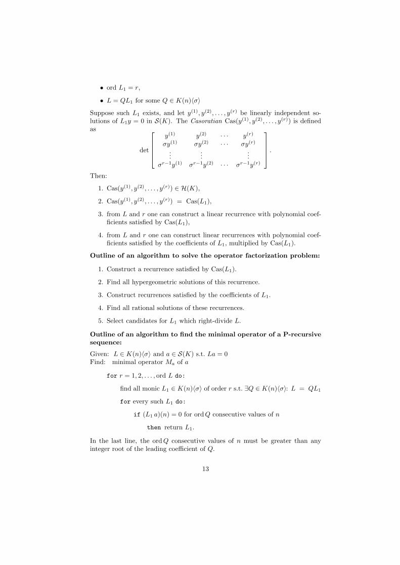
• ord L1 = r,

• L = QL1 for some Q ∈ K(n)〈σ〉

Suppose such L1 exists, and let y(1), y(2), . . . , y(r) be linearly independent so-lutions of L1y = 0 in S(K). The Casoratian Cas(y(1), y(2), . . . , y(r)) is definedas

det

y(1) y(2) · · · y(r)

σy(1) σy(2) · · · σy(r)

......

...σr−1y(1) σr−1y(2) · · · σr−1y(r)

.Then:

1. Cas(y(1), y(2), . . . , y(r)) ∈ H(K),

2. Cas(y(1), y(2), . . . , y(r)) = Cas(L1),

3. from L and r one can construct a linear recurrence with polynomial coef-ficients satisfied by Cas(L1),

4. from L and r one can construct linear recurrences with polynomial coef-ficients satisfied by the coefficients of L1, multiplied by Cas(L1).

Outline of an algorithm to solve the operator factorization problem:

1. Construct a recurrence satisfied by Cas(L1).

2. Find all hypergeometric solutions of this recurrence.

3. Construct recurrences satisfied by the coefficients of L1.

4. Find all rational solutions of these recurrences.

5. Select candidates for L1 which right-divide L.

Outline of an algorithm to find the minimal operator of a P-recursivesequence:

Given: L ∈ K(n)〈σ〉 and a ∈ S(K) s.t. La = 0Find: minimal operator Ma of a

for r = 1, 2, . . . , ord L do:

find all monic L1 ∈ K(n)〈σ〉 of order r s.t. ∃Q ∈ K(n)〈σ〉: L = QL1

for every such L1 do:

if (L1 a)(n) = 0 for ordQ consecutive values of n

then return L1.

In the last line, the ordQ consecutive values of n must be greater than anyinteger root of the leading coefficient of Q.

13

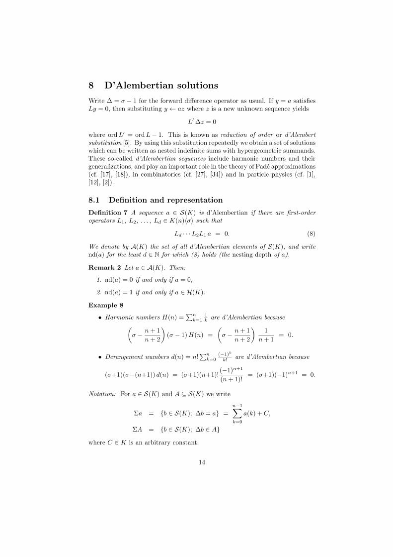
8 D’Alembertian solutions

Write ∆ = σ − 1 for the forward difference operator as usual. If y = a satisfiesLy = 0, then substituting y ← az where z is a new unknown sequence yields

L′∆z = 0

where ordL′ = ordL− 1. This is known as reduction of order or d’Alembertsubstitution [5]. By using this substitution repeatedly we obtain a set of solutionswhich can be written as nested indefinite sums with hypergeometric summands.These so-called d’Alembertian sequences include harmonic numbers and theirgeneralizations, and play an important role in the theory of Pade approximations(cf. [17], [18]), in combinatorics (cf. [27], [34]) and in particle physics (cf. [1],[12], [2]).

8.1 Definition and representation

Definition 7 A sequence a ∈ S(K) is d’Alembertian if there are first-orderoperators L1, L2, . . . , Ld ∈ K(n)〈σ〉 such that

Ld · · ·L2L1 a = 0. (8)

We denote by A(K) the set of all d’Alembertian elements of S(K), and writend(a) for the least d ∈ N for which (8) holds (the nesting depth of a).

Remark 2 Let a ∈ A(K). Then:

1. nd(a) = 0 if and only if a = 0,

2. nd(a) = 1 if and only if a ∈ H(K).

Example 8

• Harmonic numbers H(n) =∑nk=1

1k are d’Alembertian because(

σ − n+ 1

n+ 2

)(σ − 1)H(n) =

(σ − n+ 1

n+ 2

)1

n+ 1= 0.

• Derangement numbers d(n) = n!∑nk=0

(−1)kk! are d’Alembertian because

(σ+1)(σ−(n+1)) d(n) = (σ+1)(n+1)!(−1)n+1

(n+ 1)!= (σ+1)(−1)n+1 = 0.

Notation: For a ∈ S(K) and A ⊆ S(K) we write

Σa = {b ∈ S(K); ∆b = a} =

n−1∑k=0

a(k) + C,

ΣA = {b ∈ S(K); ∆b ∈ A}

where C ∈ K is an arbitrary constant.

14

Remark 3

1. ∆ + 1 = σ,

2. ∆Σ = 1,

3. σΣ = Σ + 1,

4. Σ0 = K.

Proposition 3 Let r ∈ K(n), σh = rh, and f ∈ S(K). Then

{y ∈ S(K); (σ − r)y = f} = hΣf

σh.

Proof: Assume that (σ − r)y = f and write y = h z. Then

f = (σ − r)y = (σ − r)h z = σhσz − r h z = σh∆z,

hence ∆z = fσh , so z ∈ Σ f

σh and y = h z ∈ hΣ fσh . – Conversely,

(σ − r)hΣf

σh= σhσΣ

f

σh− rhΣ

f

σh= σh∆Σ

f

σh= f.

�

Corollary 2

Ker (σ − rd) · · · (σ − r2)(σ − r1) = h1 Σh2σh1

Σh3σh2· · ·Σ hd

σhd−1Σ0 (9)

where σhi = rihi for i = 1, 2, . . . , d.

It turns out that for any L ∈ K(n)〈σ〉, the space of all d’Alembertian solu-tions of Ly = 0 is of the form

h1 Σh2 Σh3 · · ·Σhd Σ0 (10)

for some d ≤ ordL and h1, h2, . . . , hd ∈ H(K).

Example 9 (Amer. Math. Monthly problem no. 10375 – continued from Ex-ample 7)

L = σ2 − 2(2n+ 3)2σ + 4(n+ 1)2(2n+ 1)(2n+ 3),L = L2L1,L1 = σ − (2n+ 1)(2n+ 2),L2 = σ − (2n+ 2)(2n+ 3).

Since L1(2n)! = 0 and L2(2n+ 1)! = 0, it follows from (9) that

KerL = (2n)! Σ(2n+ 1)!

(2n+ 2)!Σ 0 = (2n)! Σ

C

n+ 1

= (2n)!

(n−1∑k=0

C

k + 1+D

)= C (2n)!H(n) +D (2n)!

where C,D ∈ K are arbitrary constants.

15

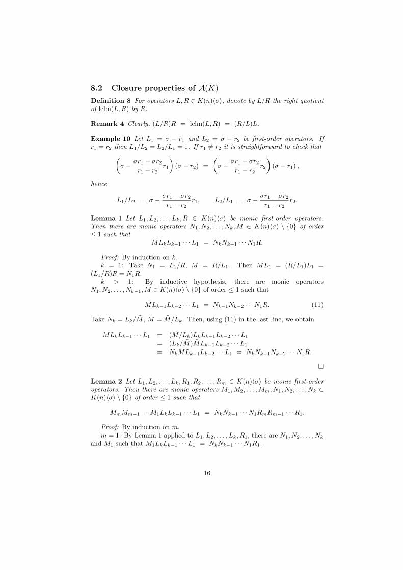
8.2 Closure properties of A(K)

Definition 8 For operators L,R ∈ K(n)〈σ〉, denote by L/R the right quotientof lclm(L,R) by R.

Remark 4 Clearly, (L/R)R = lclm(L,R) = (R/L)L.

Example 10 Let L1 = σ − r1 and L2 = σ − r2 be first-order operators. Ifr1 = r2 then L1/L2 = L2/L1 = 1. If r1 6= r2 it is straightforward to check that(

σ − σr1 − σr2r1 − r2

r1

)(σ − r2) =

(σ − σr1 − σr2

r1 − r2r2

)(σ − r1) ,

hence

L1/L2 = σ − σr1 − σr2r1 − r2

r1, L2/L1 = σ − σr1 − σr2r1 − r2

r2.

Lemma 1 Let L1, L2, . . . , Lk, R ∈ K(n)〈σ〉 be monic first-order operators.Then there are monic operators N1, N2, . . . , Nk,M ∈ K(n)〈σ〉 \ {0} of order≤ 1 such that

MLkLk−1 · · ·L1 = NkNk−1 · · ·N1R.

Proof: By induction on k.k = 1: Take N1 = L1/R, M = R/L1. Then ML1 = (R/L1)L1 =

(L1/R)R = N1R.k > 1: By inductive hypothesis, there are monic operators

N1, N2, . . . , Nk−1, M ∈ K(n)〈σ〉 \ {0} of order ≤ 1 such that

MLk−1Lk−2 · · ·L1 = Nk−1Nk−2 · · ·N1R. (11)

Take Nk = Lk/M , M = M/Lk. Then, using (11) in the last line, we obtain

MLkLk−1 · · ·L1 = (M/Lk)LkLk−1Lk−2 · · ·L1

= (Lk/M)MLk−1Lk−2 · · ·L1

= NkMLk−1Lk−2 · · ·L1 = NkNk−1Nk−2 · · ·N1R.

�

Lemma 2 Let L1, L2, . . . , Lk, R1, R2, . . . , Rm ∈ K(n)〈σ〉 be monic first-orderoperators. Then there are monic operators M1,M2, . . . ,Mm, N1, N2, . . . , Nk ∈K(n)〈σ〉 \ {0} of order ≤ 1 such that

MmMm−1 · · ·M1LkLk−1 · · ·L1 = NkNk−1 · · ·N1RmRm−1 · · ·R1.

Proof: By induction on m.m = 1: By Lemma 1 applied to L1, L2, . . . , Lk, R1, there are N1, N2, . . . , Nk

and M1 such that M1LkLk−1 · · ·L1 = NkNk−1 · · ·N1R1.

16

m > 1: By inductive hypothesis applied to R1, R2, . . . , Rm−1, there aremonic operators M1,M2, . . . ,Mm−1, N1, N2, . . . , Nk ∈ K(n)〈σ〉 \ {0} of order≤ 1 such that

Mm−1Mm−2 · · ·M1LkLk−1 · · ·L1 = NkNk−1 · · · N1Rm−1Rm−2 · · ·R1. (12)

By Lemma 1 applied to N1, N2, . . . , Nk, Rm, there are N1, N2, . . . , Nk and Mm

such thatMmNkNk−1 · · · N1 = NkNk−1 · · ·N1Rm,

hence, by multiplying (12) with Mm from the left, we obtain

MmMm−1 · · ·M1LkLk−1 · · ·L1 = MmNkNk−1 · · · N1Rm−1Rm−2 · · ·R1

= NkNk−1 · · ·N1RmRm−1 · · ·R1.

�

Proposition 4 A(K) is closed under addition.

Proof: Let a, b ∈ A(K). Then there are monic first-order operatorsL1, L2, . . . , Lk, R1, R2, . . . , Rm ∈ K(n)〈σ〉 such that

LkLk−1 · · ·L1a = RmRm−1 · · ·R1b = 0.

By Lemma 2, there are monic operators M1, . . . ,Mm, N1, . . . , Nk ∈ K(n)〈σ〉 \{0} of order ≤ 1 such that

L := MmMm−1 · · ·M1LkLk−1 · · ·L1 = NkNk−1 · · ·N1RmRm−1 · · ·R1.

Then La = Lb = 0, so L(a+ b) = 0 and a+ b ∈ A(K). �

Proposition 5 A(K) is closed under multiplication.

Proof: Let a, b ∈ A(K). We show that ab ∈ A(K) by induction on the sumof their nesting depths nd(a) + nd(b).

a) nd(a) = 0 or nd(b) = 0: In this case one of a, b is 0, hence ab = 0 ∈ A(K).b) nd(a),nd(b) ≥ 1: By (10) we can write a ∈ h1 Σh2 Σh3 · · ·Σhd Σ0 and

b ∈ g1 Σg2 Σg3 · · ·Σge Σ0 where hi, gj ∈ H(K), d = nd(a), and e = nd(b). Leta1 = h2 Σh3 · · ·Σhd Σ0 and b1 = g2 Σg3 · · ·Σge Σ0, so that a ∈ h1 Σa1 andb ∈ g1 Σb1 with a1, b1 ⊆ A(K), nd(a1) < nd(a) and nd(b1) < nd(b). Clearlyha ∈ A(K) whenever h ∈ H(K) and a ∈ A(K), hence it suffices to show that(∑a1)g1

∑b1 ⊆ A(K). Using the product rule of difference calculus

∆uv = u∆v + ∆uσv

and Remark 3 repeatedly, we obtain

∆(

(∑

a1)g1∑

b1

)= (

∑a1)g1∆

∑b1 + ∆((

∑a1)g1)σ

∑b1

= (∑a1)g1b1 + ((

∑a1)∆g1 + a1σg1)(

∑b1 + b1)

= ∆g1(∑a1)∑b1 + (g1 + ∆g1)b1

∑a1 + a1σg1(

∑b1 + b1)

= ∆g1(∑a1)∑b1 + σg1(a1

∑b1 + b1

∑a1 + a1b1).

17

Assume first that g1 = 1. Then ∆ ((∑a1)∑b1) = a1

∑b1 +b1

∑a1 +a1b1. By

inductive hypothesis and from Proposition 4 it follows that a1∑b1 + b1

∑a1 +

a1b1 ⊆ A(K). Therefore there are first-order operators L1, L2, . . . , Lk ∈K(n)〈σ〉 such that

LkLk−1 · · ·L1∆ ((∑a1)∑b1) = 0,

hence (∑a1)∑b1 ⊆ A(K). In the general case, ∆g1, σg1 ∈ H(K) now implies

∆ ((∑a1)g1

∑b1) ⊆ A(K). Again we conclude that (

∑a1)g1

∑b1 ⊆ A(K). �

Proposition 6 A(K) is closed under σ and σ−1.

Proof: Let a ∈ A(K). Then there are monic first-order operatorsL1, L2, . . . , Lk ∈ K(n)〈σ〉 such that LkLk−1 · · ·L1a = 0.

By Lemma 1 with R = σ, there are monic operators N1, N2, . . . , Nk,M ∈K(n)〈σ〉 \ {0} of order ≤ 1 such that MLkLk−1 · · ·L1 = NkNk−1 · · ·N1σ.Hence

NkNk−1 · · ·N1σa = MLkLk−1 · · ·L1a = 0,

so σa ∈ A(K).From LkLk−1 · · ·L1a = 0 it follows that LkLk−1 · · ·L1σ(σ−1a) = 0, hence

σ−1a ∈ A(K) as well. �

Theorem 9 A(K) is a difference ring.

Proof: This follows from Propositions 4, 5 and 6. �

Corollary 3 A(K) is the least subring of S(K) which contains H(K) and isclosed under σ, σ−1, and Σ.

Proof: Denote by HS(K) the least subring of S(K) which contains H(K)and is closed under σ, σ−1, and Σ.

By Corollary 2, every a ∈ A(K) is obtained from 0 by using Σ and multipli-cation with elements from H(K). Hence A(K) ⊆ HS(K).

Conversely, A(K) is closed under σ and σ−1 by Proposition 6, and under Σby Corollary 2. Since A(K) is a subring of S(K) containing H(K), it followsthat HS(K) ⊆ A(K). �

Proposition 7 A(K) is closed under multisection.

Proof: Let a ∈ A(K). We show that any multisection of a belongs to A(K)by induction on the nesting depth nd(a) of a.

a) nd(a) = 0: In this case a = 0, so the assertion holds.b) nd(a) ≥ 1: By (10) we can write a ∈ h1 Σh2 Σh3 · · ·Σhd Σ0 where d =

nd(a) and h1, h2, . . . , hd ∈ H(K). Let h = h1 and b = h2 Σh3 · · ·Σhd Σ0, sothat a ∈ hΣb where b ⊆ A(K) and nd(b) < nd(a).

18

Let c ∈ S(K), defined by c(n) = a(mn + r) for all n ∈ N, where m, r ∈ N,m ≥ 2, 0 ≤ r < m, be a multisection of a. Then for all n ∈ N

c(n) = a(mn+ r) = h(mn+ r)

mn+r−1∑k=0

b(k)

= h(mn+ r)

m−1∑i=0

n−1∑j=0

b(mj + i) +

r−1∑i=0

b(mn+ i)

= hm,r(n)

m−1∑i=0

n−1∑j=0

bm,i(j) +

r−1∑i=0

bm,i(n)

where hm,r(n) = h(mn+ r) and bm,i(n) = b(mn+ i) for 0 ≤ i < m. Hence

c = hm,r

(m−1∑i=0

Σbm,i +

r−1∑i=0

bm,i

)

where hm,r ∈ H(K) ⊆ A(K) by Proposition 1, and bm,i ∈ A(K) by inductivehypothesis as a multisection of b. Since A(K) is closed under Σ, addition andmultiplication, it follows that c ∈ A(K). �

8.3 Finding d’Alembertian solutions

The following theorem provides a way to find d’Alembertian solutions of Ly = 0.

Theorem 10 Ly = 0 has a nonzero d’Alembertian solution if and only if Ly =0 has a hypergeometric solution.

For a proof, see [10].

Outline of an algorithm for finding the space of all d’Alembertiansolutions:

1. Find a hypergeometric solution h1 of Ly = 0.If none exists then return 0 and stop.

2. Let L1 = σ − σh1

h1. Right-divide L by L1 to obtain L = QL1.

3. Recursively use the algorithm on Qy = 0. Let the output be a.

4. Return h1 Σ aσh1

and stop.

A much more general algorithm which finds solutions in ΠΣ∗-difference ex-tension fields of (K(n), σ) is presented in [32]. For the relevant theory, see [33],[35], [36], [37].

19

9 Liouvillian solutions

Definition 9 L(K) is the least subring of S(K) containing H(K), closed under

• σ, σ−1,

• Σ,

• interlacing of an arbitrary number of sequences.

The elements of L(K) are Liouvillian sequences.

Example 11 The sequence

n!! =

{2kk!, n = 2k,(2k+1)!2kk!

, n = 2k + 1

is Liouvillian (as an interlacing of two hypergeometric sequences ).

The following theorem provides a way to find Liouvillian solutions of Ly = 0.

Theorem 11 Ly = 0 has a nonzero Liouvillian solution if and only if Ly = 0has a solution which is an interlacing of at most ordL hypergeometric sequences.

For a proof, see [21]. For algorithms to find Liouvillian solutions, see [13],[25], [8], [14], [15], [24], [19], [20].

Theorem 12 A sequence in S(K) is Liouvillian if and only if it is an inter-lacing of d’Alembertian sequences.

This is proved in [31] as a corollary of the results of [21] obtained by meansof Galois theory of difference equations. Here we give a self-contained proofbased on closure properties of interlacings of d’Alembertian sequences.

Let Λ(a0, a1, . . . , ak−1), or Λk−1j=0aj , denote the interlacing of a0, a1, . . . , ak−1.By definition of interlacing we have(

Λk−1j=0aj)

(n) = Λ(a0, a1, . . . , ak−1)(n) = an mod k(n div k)

for all n ∈ N, where

n div k =⌊nk

⌋, n mod k = n−

⌊nk

⌋k.

Denote temporarily the set of all interlacings of (one or more) d’Alembertiansequences by AL(K). The goal is to prove that AL(K) = L(K).

Proposition 8 AL(K) ⊆ L(K).

Proof: Since H(K) ⊆ L(K) and L(K) is a ring closed under Σ, we haveA(K) ⊆ L(K). Since L(K) is closed under interlacing, AL(K) ⊆ L(K). �

20

Lemma 3 AL(K) is closed under addition and multiplication.

Proof: Let � denote either addition or multiplication in K and S(K). Weclaim that, for k,m ∈ N and a0, a1, . . . , ak−1, b0, b1, . . . , bm−1 ∈ A(K), we have(

Λk−1j=0aj)�(Λm−1j=0 bj

)= Λkm−1`=0 (a`,k,m � b`,k,m) (13)

where for all n ∈ N,

a`,k,m(n) = a` mod k(mn+ ` div k),

b`,k,m(n) = b` mod m(kn+ ` div m).

Indeed,(Λkm−1`=0 (a`,k,m � b`,k,m)

)(n)

= an mod km,k,m(n div km)� bn mod km,k,m(n div km) = u� v

where

u = a(n mod km) mod k(m(n div km) + (n mod km) div k),

v = b(n mod km) mod m(k(n div km) + (n mod km) div m).

From

(n mod km) mod k =(n−

⌊ n

km

⌋km)

mod k = n mod k,

(n mod km) mod m =(n−

⌊ n

km

⌋km)

mod m = n mod m,

m(n div km) + (n mod km) div k = m⌊ n

km

⌋+

⌊n−

⌊nkm

⌋km

k

⌋=⌊nk

⌋= n div k,

k(n div km) + (n mod km) div m = k⌊ n

km

⌋+

⌊n−

⌊nkm

⌋km

m

⌋=⌊ nm

⌋= n div m

it follows that

u� v = an mod k(n div k)� bn mod m(n div m)

=(Λk−1j=0aj

)(n)�

(Λm−1j=0 bj

)(n) =

((Λk−1j=0aj

)�(Λm−1j=0 bj

))(n),

proving (13). By Proposition 7, the sequences a`,k,m and b`,k,m belong toA(K). Since A(K) is a ring, the right-hand side of (13) is an interlacing ofd’Alembertian sequences, and hence so is the left-hand side. �

Lemma 4 AL(K) is closed under σ and σ−1.

21

Proof: Let a0, a1, . . . , ak−1 be d’Alembertian sequences. Then:(σ(Λk−1j=0aj

))(n) =

(Λk−1j=0aj

)(n+ 1)

= a(n+1) mod k((n+ 1) div k)

=

{an mod k+1(n div k), n mod k 6= k − 1,a0(n div k + 1), n mod k = k − 1

=

{an mod k+1(n div k), n mod k 6= k − 1,(σa0)(n div k), n mod k = k − 1

=(Λk−1j=0 bj

)(n)

where

bj =

{aj+1, j 6= k − 1,σa0, j = k − 1.

By Proposition 6, b0, b1, . . . , bk−1 are d’Alembertian. So σ(Λk−1j=0aj

)= Λk−1j=0 bj

is an interlacing of d’Alembertian sequences.Similarly,(

σ−1(Λk−1j=0aj

))(n) =

(Λk−1j=0aj

)(n− 1)

= a(n−1) mod k((n− 1) div k)

=

{an mod k−1(n div k), n mod k 6= 0,ak−1(n div k − 1), n mod k = 0

=

{an mod k−1(n div k), n mod k 6= 0,(σ−1ak−1)(n div k), n mod k = 0

=(Λk−1j=0 cj

)(n)

where

cj =

{aj−1, j 6= 0,σ−1ak−1, j = 0.

By Proposition 6, c0, c1, . . . , ck−1 are d’Alembertian. So σ−1(Λk−1j=0aj

)= Λk−1j=0 cj

is an interlacing of d’Alembertian sequences. �

Lemma 5 AL(K) is closed under Σ.

Proof: Let a0, a1, . . . , ak−1 be d’Alembertian sequences. We claim that

Σ(Λk−1j=0aj

)= Λk−1j=0

j−1∑i=0

σΣai +

k−1∑i=j

Σai

. (14)

22

Indeed, for all n ∈ N,(Σ(Λk−1j=0aj

))(n)

=

n−1∑`=0

(Λk−1j=0aj

)(`) =

n−1∑`=0

a` mod k(` div k)

=

(n−1) mod k∑i=0

bn−1k c∑j=0

ai(j) +

k−1∑i=(n−1) mod k+1

bn−1k c−1∑j=0

ai(j) (15)

=

n mod k−1∑i=0

bnk c∑j=0

ai(j) +

k−1∑i=n mod k

bnk c−1∑j=0

ai(j) (16)

=

n mod k−1∑i=0

(σΣai) (n div k) +

k−1∑i=n mod k

(Σai) (n div k)

=

Λk−1j=0

j−1∑i=0

σΣai +

k−1∑i=j

Σai

(n),

proving (14). Here equality in (15) follows by mapping each ` ∈ {0, 1, . . . , n−1}to the pair (i, j) = (` mod k, ` div k) and summing over all the resulting pairs,and equality in (16) follows by noting that when n mod k 6= 0, we have

(n− 1) mod k = n mod k − 1,

(n− 1) div k = n div k,

while for n mod k = 0, both (15) and (16) are equal to∑k−1i=0

∑nk−1j=0 ai(j).

Since A(K) is closed under Σ, σ and addition, the right-hand side of (14) isan interlacing of d’Alembertian sequences, and hence so is the left-hand side. �

Lemma 6 AL(K) is closed under interlacing.

Proof: An arbitrary interlacing can be obtained by using addition, shifts,and interlacing of zero sequences with a single non-zero sequence by the formula

Λ(a0, a1, . . . , ak−1) =

k−1∑i=0

σiΛ(0, 0, . . . , 0, ak−1−i).

Hence, by Propositions 3 and 4, it suffices to show that AL(K) is closed underinterlacing of zero sequences with a single non-zero sequence from AL(K). Butthis is immediate: Let a0, a1, . . . , ak−1 be d’Alembertian sequences. Then theinterlacing of m zero sequences with Λ(a0, a1, . . . , ak−1)

Λ(0, 0, . . . , 0,Λ(a0, a1, . . . , ak−1))

= Λ(0, 0, . . . , 0, a0, 0, 0, . . . , 0, a1, . . . , 0, 0, . . . , 0, ak−1)

23

is an interlacing of mk + k d’Alembertian sequences. �

Proof of Theorem 12. By Proposition 8, it suffices to show that L(K) ⊆ AL(K).This is true since by Lemmas 3 – 6, AL(K) is a subring of S(K) containingH(K) and closed under σ, σ−1, Σ and interlacing, while L(K) is the least suchring. �

References

[1] Ablinger, J., Blumlein, J., Schneider, C.: Harmonic sums and polylog-arithms generated by cyclotomic polynomials, J. Math. Phys. 52, 1–52(2011)

[2] Ablinger, J., Blumlein, J., Schneider, C.: Analytic and algorithmic aspectsof generalized harmonic sums and polylogarithms, submitted, 75 pages(2013)

[3] Abramov, S.A.: Problems in computer algebra that are connected with asearch for polynomial solutions of linear differential and difference equa-tions, Moscow Univ. Comput. Math. Cybernet. 3, 63–68 (1989). Transl.from Vestn. Moskov. univ. Ser. XV. Vychisl. mat. kibernet. 3, 56–60 (1989)

[4] Abramov, S.A.: Rational solutions of linear differential and differenceequations with polynomial coefficients, U.S.S.R. Comput. Maths. Math.Phys. 29, 7–12 (1989). Transl. from Zh. vychisl. mat. mat. fyz. 29, 1611–1620 (1989)

[5] Abramov, S.A.: On d’Alembert substitution, Proc. ISSAC’93, Kiev, 20–26(1993)

[6] Abramov, S.A.: Rational solutions of linear difference and q-differenceequations with polynomial coefficients, Programming and Comput. Soft-ware, 21, 273–278 (1995). Transl. from Programmirovanie 21, 3–11 (1995)

[7] Abramov, S.A., Barkatou, M.A.: Rational solutions of first order lineardifference systems, Proc. ISSAC’98, Rostock, 124–131 (1998)

[8] Abramov, S.A., Barkatou, M.A., Khmelnov, D.E.: On m-interlacing so-lutions of linear difference equations, Proc. CASC’09, Kobe, LNCS 5743,Springer, 1–17 (2009)

[9] Abramov, S.A., Bronstein, M., Petkovsek, M.: On polynomial solutions oflinear operator equations, Proc. ISSAC’95, Montreal, 290–296 (1995)

[10] Abramov, S.A., Petkovsek, M.: D’Alembertian solutions of linear operatorequations, Proc. ISSAC’94, Oxford, 169–174 (2004)

[11] Apagodu, M., Zeilberger, D.: Multi-variable Zeilberger and Almkvist-Zeilberger algorithms and the sharpening of Wilf-Zeilberger theory, Adv.in Appl. Math. 37, 139–152 (2006)

24

[12] Blumlein, J., Klein, S., Schneider, C., Stan, F.: A symbolic summationapproach to Feynman integral calculus, J. Symbolic Comput. 47, 1267–1289 (2012)

[13] Bomboy, R.: Liouvillian solutions of ordinary linear difference equations,Proc. CASC’02, Simeiz (Yalta), 17–28 (2002)

[14] Cha, Y., van Hoeij, M.: Liouvillian solutions of irreducible linear differenceequations, Proc. ISSAC’09, Seoul, 87–94 (2009)

[15] Cha, Y., van Hoeij, M., Levy, G.: Solving recurrence relations using localinvariants, Proc. ISSAC’10, Munchen, 303–309 (2010)

[16] Cluzeau, T., van Hoeij, M.: Computing hypergeometric solutions of linearrecurrence equations, Appl. Algebra Engrg. Comm. Comput. 17, 83–115(2006)

[17] Driver, K., Prodinger, H., Schneider, C., Weideman, J.A.C.: Pade ap-proximations to the logarithm. II. Identities, recurrences, and symboliccomputation, Ramanujan J. 11, 139–158 (2006)

[18] Driver, K., Prodinger, H., Schneider, C., Weideman, J.A.C.: Pade approx-imations to the logarithm. III. Alternative methods and additional results,Ramanujan J. 12, 299–314 (2006)

[19] Feng, R., Singer, M.F., Wu, M.: Liouvillian solutions of linear difference-differential equations, J. Symbolic Comput. 45, 287–305 (2010)

[20] Feng, R., Singer, M.F., Wu, M.: An algorithm to compute Liouvilliansolutions of prime order linear difference-differential equations, J. SymbolicComput. 45, 306–323 (2010)

[21] Hendriks, P.A., Singer, M.F.: Solving difference equations in finite terms,J. Symbolic Comput. 27, 239–259 (1999)

[22] van Hoeij, M.: Rational solutions of linear difference equations, Proc.ISSAC’98, Rostock, 120–123 (1998)

[23] van Hoeij, M.: Finite singularities and hypergeometric solutions of linearrecurrence equations, J. Pure Appl. Algebra 139, 109–131 (1999)

[24] van Hoeij, M., Levy, G.: Liouvillian solutions of irreducible second orderlinear differential equations, Proc. ISSAC’10, Munchen, 297–301 (2010)

[25] Khmelnov, D.E.: Search for Liouvillian solutions of linear recurrence equa-tions in MAPLE computer algebra system, Program. Comput. Softw. 34,204–209 (2008)

[26] Larson, R.G., Taft, E.J.: The algebraic structure of linearly recursive se-quences under Hadamard product, Israel J. Math. 72, 118–132 (1990)

25

[27] Paule, P., Schneider, C.: Computer proofs of a new family of harmonicnumber identities, Adv. in Appl. Math. 31, 359–378 (2003)

[28] Petkovsek, M.: Hypergeometric solutions of linear recurrences with poly-nomial coefficients, J. Symbolic Comput. 14, 243–264 (1992)

[29] Petkovsek, M., Wilf, H.S., Zeilberger, D.: A = B, A K Peters, Wellesley,MA (1996)

[30] van der Put, M., Singer, M.F.: Galois Theory of Difference Equations,Springer-Verlag, Berlin (1997)

[31] Reutenauer, C.: On a matrix representation for polynomially recursivesequences, Electron. J. Combin. 19(3), P36 (2012)

[32] Schneider, C.: The summation package Sigma: underlying principles anda rhombus tiling application, Discrete Math. Theor. Comput. Sci. 6 (elec-tronic), 365–386 (2004)

[33] Schneider, C.: Solving parameterized linear difference equations in termsof indefinite nested sums and products, J. Difference Equ. Appl. 11, 799–821 (2005)

[34] Schneider, C.: Symbolic summation assists combinatorics, Sem. Lothar.Combin. 56, Art. B56b (electronic), 36 pp. (2006/07)

[35] Schneider, C.: Simplifying sums in ΠΣ∗-extensions, J. Algebra Appl. 6,415–441 (2007)

[36] Schneider, C.: A refined difference field theory for symbolic summation,J. Symbolic Comput. 43, 611–644 (2008)

[37] Schneider, C.: Structural theorems for symbolic summation, Appl. AlgebraEngrg. Comm. Comput. 21, 1–32 (2010)

[38] Stanley, R.P.: Enumerative Combinatorics, Vol. 1, Cambridge UniversityPress, Cambridge (1997)

[39] Stanley, R.P.: Differentiably finite power series, European J. Combin. 1,175 –188 (1980)

[40] Stanley, R.P.: Enumerative Combinatorics, Vol. 2, Cambridge UniversityPress, Cambridge (1999)

[41] Zeilberger, D.: A fast algorithm for proving terminating hypergeometricidentities, Discrete Math. 80, 207–211 (1990)

[42] Zeilberger, D.: The method of creative telescoping, J. Symbolic Comput.11, 195–204 (1991)

26