Solving Large Scale Optimization Problems using CPLEX Optimization Studio
22
Alkis Vazacopoulos Robert Ashford Optimization Direct Optimization Direct, CPLEX and Very Large Optimization Models
-
Upload
optimizatiodirectdirect -
Category
Data & Analytics
-
view
659 -
download
2
Transcript of Solving Large Scale Optimization Problems using CPLEX Optimization Studio
Alkis Vazacopoulos
Robert Ashford
Optimization Direct
Optimization Direct, CPLEX and
Very Large Optimization Models

Summary
• Introduce Optimization Direct Inc.
• Explain what we do
• Look at getting the most from optimization
• some modeling issues
• optimizer issues
• Example of large scale optimization:
scheduling heuristic

Optimization Direct
• IBM Business Partner
• Sell CPLEX optimization Studio
• More than 30 years of experience in developing and selling
Optimization software
• Experience in implementing optimization technology in all the
verticals
• Sold to end users – Fortune 500 companies
• Train our customers to get the maximum out of the IBM
software
• Help the customers get a flying start and get the most from
optimization and the software right away

Background
• Robert Ashford
• Robert co-founded Dash Optimization in 1984. Helped pioneer the development of new modeling and solution technologies – the first integrated development environment for optimization – in the forefront of technology development driving the size, complexity and scope of applications. Dash was sold in 2008 and Robert continued leading development within Fair Isaac until the Fall of 2010, Dr. Ashford subsequently, co-founded Optimization Direct in 2014.
• Alkis Vazacopoulos
• Alkis is a Business Analytics and Optimization expert. From January 2008 to January 2011 he was Vice President at FICO Research. Prior to that he was the President at Dash Optimization, Inc. where he worked closely with end users, consulting companies, OEMs/ISVs in developing optimization solutions.

Get more from Optimization
• Modeling
• Use modeling language and ‘Developer Studio’
environment
• Such as OPL and CPLEX Optimization Studio
• Easier to build, debug, manage models
• Exploit (data) sparsity
• Keep formulations tight
• Optimization
• Many models solve out-of-the-box
• Others (usually large) models do not
• Tune optimizer
• Distributed MIP
• Use Heuristics

Modeling: Use Sparsity
Avoid unnecessary looping: example of network model
Xsdij = traffic on link (i,j) from route (s,d)
Σj Xsdlj - Σi Xsdil = 0, for all s,d,l ϵ {Nodes}
Coded as:
int NbNodes = ...;
range Nodes = 1..NbNodes;
dvar float+ X[Nodes][Nodes][Nodes][Nodes] = ...;
forall(s in Nodes, d in Nodes, l in Nodes : s != d && s != l && d != l)
XFlow:
sum(j in Nodes) X[s][d][l][j] – sum(i in Nodes) X[s][d][i][l] == 0;
is inefficient: loops over all combinations

Modeling: Use Sparsity
More efficient: only loop over existent links and routes
Xkl = traffic on link l from route k
Σj: (n,j) ϵ {links} Xk(n,j) - Σi: (i,n) ϵ {links} Xk(I,n) = 0, all k ϵ {Links}, n ϵ {Nodes}
coded asint NbNodes = ...;
range Nodes = 1..NbNodes;
tuple link { int s; int d;}
{link} Links = ...;
dvar float+ X[Links][Links];
forall( k in Links, n in Nodes : n != k.s && n != k.d )
XFlow:
sum(<n,j> in Links) X[k][<n,j>]
– sum(<i,n> in Links) X[k][<i,n>] == 0;

Tight Formulations
• Make LP feasible region as small as possible whilst
containing integer feasible points
• ‘big-M’/indicator constraints well known:
• y - M x ≤ 0, y ≥ 0, s binary. Identify directly to solver.
• Take care with others. Customer example: xi binary
2 x1 + 2 x2 + x3 + x4 ≤ 3 is worse than
x1 + x2 ≤ 1 and x1 + x2 + x3 + x4 ≤ 2
2 x1 + 2 x2 + x3 + x4 ≤ 2 is worse than
x1 + x2 ≤ 1 and x1 + x2 + x3 + x4 ≤ 1

Driving the Optimizer
• Performance of modern commercial software and hardware in a different league from ten years ago
• Hardware
• Around 10 X faster than 10 years ago
• Depends on characteristic of interest
• Software
• CPLEX leads
• 100X ~ 1000X faster than best open source
• Tunable to specific model classes
• Exploits multiple processor cores
• Exploits multiple machine clusters

Hardware characteristics
1990 2005 2014 Improvement
IBM PS/2 80-111 Intel Pentium 4 540 Intel i7-4790K
Processor speed 20 MHz 3.2 GHz 4.4GHz 220
Cores 1 1 4 4
Time for a FP multiply 1.4 – 2.8 ms. 0.08†
– 0.3 ns. 0.008†
– 0.2 ns. 7,000 – 350,000†
Typical memory size 4 Mbyte 2 GByte 16 GByte 4000
Memory speed 85 ns. 45 ns. 12 ns 7
L2 cache size None 1 Mbyte 8 Mbyte
Typical disk capacity 115 Mbyte 120 GByte 1 TByte 9,000
† using the vector facility.

CPLEX Performance Improvements

Where’s the Problem?
• Many models now solved routinely which would have
been impossible (‘unsolvable’) a few years ago
• BUT: have super-linear growth of solving effort as model
size/complexity increases
• AND: customer models keep getting larger
• Globalized business has larger and more complex supply
chain
• Optimization expanding into new areas, especially
scheduling
• Detailed models easier to sell to management and end-
users

Getting more difficult
• Solver has to
• (Presolve and) solve LP relaxation
• Find and apply cuts
• Branch on remaining infeasibilities (and find and apply cuts too)
• Look for feasible solutions with heuristics all the while
• Simplex relaxation solves theoretically NP, but in practice effort increases between linearly and quadratic
• Barrier solver effort grows more slowly, but:• cross-over still grows quickly
• usually get more integer infeasibilities
• can’t use last solution/basis to accelerate
• Cutting grows faster than quadratic: each cuts requires more effort, more cuts/round, more rounds of cuts, each round harder to apply.
• Branching is exponential: 2n in number of (say) binaries n
What can we do? Tuning the Optimizer
• Models usually solved many times
• Repeat planning or scheduling process
• Solve multiple scenarios
• Good algorithms for dynamic parameter/strategy choice
• Expert analysis may do even better trading off solution time and optimality level:
• LP algorithm choice
• Kind of cuts and their intensity
• Heuristic choice, effort and frequency
• Branching strategies and priorities
• Use more parallelism: more cores, distributed computers
• Sophisticated auto tuner for small/medium sized models

Model/Application Specific Solution
Techniques
• Proof of optimality (say to 1%) may be impractical
• Want good solutions to (say) 20%
• Solve smaller model(s)
• Heuristic approach used e.g. by RINS and local branching
• Use knowledge of model structure to break it down into
sub-models and combine solutions
• Prove solution quality by a very aggressive root solve
of whole model
Example: Large Scale Scheduling model
• Schedule 800 entities over 70 periods
• Have target number of active periods for each entity
• Entities have mutual interactions within each period
• 94K variables, 213K constraints, 93K binaries
• No usable (say within 30% gap) solution after 2 days
run time on fastest hardware (Intel i7 4790K ‘Devil’s
Canyon’)

Heuristic Solution Approach
• Solves sequence of sub-models
• Delivers usable solutions (12%-16% gap)
• Takes 4-12 hours run time
• Multiple instances can be run concurrently with
different seeds
• Can run on only 2 cores
• Can interrupt at any point and take best solution so far

Scheduling Model Heuristic Behavior
1480
743
411
239185170163159151146145143142140139138136134133129128126125124123122121120 117 116
1480
706
371
231186176166156148146143135134132131130129128127126125124123122 119
0
200
400
600
800
1000
1200
1400
1600
0 50 100 150 200 250 300 350 400
So
luti
on
Va
lue
s
Time in Minutes
5678
1234
Parallel Heuristic Approach
• Run several instances with different seeds simultaneously
• CPLEX callable library very flexible, so
• Exchange solution information between runs
• Kill sub-model solves when done better elsewhere
• Improves sub-model selection
• 4 instances run on 4 core i7-4790K
• Each instance slower than serial case which mostly used 2 cores each
• Outweighed by information exchange
• Could easily implement on clusters of computers

Parallel Heuristic Behavior
1480141414031400
817801800757
519476
320275225211210198183167166159149147140138137136135131130129127 126124123122121
118 117 115
1480
706
371
231186176166156148146143135134132131130129128127126125124123 122 119
0
200
400
600
800
1000
1200
1400
1600
0 50 100 150 200 250 300 350 400
So
luti
on
s
Time in Minutes
Parallel Serial
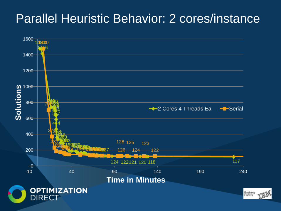
Parallel Heuristic Behavior: 2 cores/instance
14801416
743739737724692690689643641587
464
358337319293288245244243
192191190187173170167164163161159152146142141140136132130129127
124 122121 120 118 117
1480
706
371
231186176166156148146 143 135134132131130129
128
126
125
124
123
122
0
200
400
600
800
1000
1200
1400
1600
-10 40 90 140 190 240
So
luti
on
s
Time in Minutes
2 Cores 4 Threads Ea Serial

Thanks for listening
Robert Ashford
www.optimizationdirect.com