Solving Laplace Equation Problems Using DCALCdcalc.us/Tutorials/Chapter11.pdfStructural engineers...

Solving Laplace Equation Problems Using DCALC

p.11-1

Chapter 11: Solving Laplace Equation Problems Using DCALC By Karl Hanson, S.E., P.E.*

August 2013 11.1 Introduction: One of most interesting, reoccurring physical phenomena in nature is described by the Laplace equation. Mathematically, this equation is,

∂2ϕ/∂x2 + ∂2ϕ/∂y2 = 0 The Laplace equation is particularly important for solving the following types of problems:

Hydraulics Aerodynamics Torsional stresses

Pierre-Simon Laplace (1749-1827)

Why should structural engineers be interested in solving problems of this type?: Structural engineers design buildings for wind loads as mandated by building codes, typically requiring ASCE 7. Unfortunately, applying prescriptive design codes does not provide us with knowledge about how the wind flows around a structure. To really appreciate how wind forces develop against a structure, wind flow needs to be seen, in an actual wind tunnel test - or a simulation program. Recently I was involved in the proposal for a pipe suspension bridge. We were particularly interested in how vortex shedding would develop around the structure and the period of vortex shedding, so that we could check for structural resonance. Searching the Web, there are several commercially available aerodynamic modeling programs. Some of these programs are costly. Amazingly, some are free and open source, such as “OPENFOAM”, which runs under the Linux operating system, and has a strong following of users. Out of curiosity, I began to fill in my knowledge cap, learning the field of Computational Fluid Dynamics. As I got into it, the idea of writing a wind tunnel simulation program for DCALC seemed “doable”. As usual, the objective was to have something that can be easily used by structural engineers. This paper will explain the following topics:

Theory behind the Laplace equation How the Laplace equation can be solved using finite difference equations How the Laplace (and Poisson) equations can be solved for aerodynamic

problems How the Laplace equation can be solved for hydraulic seepage problems How the Laplace equation can be solved to compute torsion properties

(* http://www.designcalcs.com)


p.11-2

11.1 Theory: “What Goes In Must Come Out” We will derive the Laplace equation using an example from fluid mechanics. The continuity equation will be derived for a 2D incompressible flow field, as shown below.

By “incompressible”, we mean that the mass entering the control surface does not accumulate within the control surface. If mass were to accumulate, the density would increase with time. “u” and “v” represent the velocity components in the x and y direction. Balancing flow going into the differential control surface with flow going out of the control surface, Flow going into control surface, Qin =u*dy + v*dx Flow leaving control surface, Qout = (u + ∂u/∂x*dx)*dy

+ (v + ∂v/∂y*dy )*dx u*dy + v*dx = (u + ∂u/∂x*dx)*dy + (v + ∂v/∂y*dy )*dx ∂u/∂x + ∂v/∂y = 0 (Equation 1)

Equation 1 is the continuity equation for incompressible flow. Next, we introduce a new variable, “f”, called “velocity potential”, with the following properties,

u=∂f/∂x

and v=∂f/∂y Substituting the above into Equation 1,

∂(∂f/∂x )/∂x + ∂(∂f/∂y) /∂y = 0

∂2ϕ/∂x2 + ∂2ϕ/∂y2 = 0 (Laplace Equation)


p.11-3

11.2 Solving Partial Differential Equations Using Computational Fluid Dynamics The Laplace equation is a partial differential equation (PDE). In general, partial differential equations are difficult to solve for real-world boundary conditions. Typically, only a few closed formed solutions are available for partial differential equations, many of which have no practical use. The field of Computation Fluid Dynamics (CFD) has developed methods that can, at least in principle, be applied to any set of differential equations. These methods use the concept of discretization: “Discretization can be understood as replacement of an exact solution of PDE or a system of PDEs in a continuum domain by an approximate numerical solution in a discrete domain. Instead of continuous distributions of solution variables we find a finite set of numerical values that represents an approximation of the solution.” (Ref. 1, p. 47) These methodologies are similar to those used in the Finite Element Method. The main difference is, FEM solves simultaneous equations by matrix inversion, whereas CFD solves the equations iteratively. FEM requires a huge amount of storage space for matrix operations. CFD requires little storage space, using a minimal amount of code. The only sacrifice is the time required to iterate a stable solution. However, with today’s extremely fast computers, time really is no longer much of an issue. 11.3 Applying the Finite Difference Method to the Laplace Equation We begin by discretizing a space into equally spaced nodes:

The above shows a relatively small grid using 10 columns x 8 rows, for illustration purposes only. Note the indices are (I%,J%), using Visual Basic’s “%” sign for integer.


p.11-4

DCALC divides the screen area into 150 columns x 100 rows = 15,000 nodes:

We need to solve something involving the Laplace Equation. For this illustration, we will solve for air velocities and pressures around a house. Let’s assume that the above grid represents 80 feet.

We “draw” the house (actually the program draws). Only the nodes in the air will be used for this analysis. The program will need to identify which nodes are air and which are solid.


p.11-5

You will notice that the roof of the house is drawn in stepped nodes, rather than inclined spacing. This is done to simplify the calculation. Although it is possible to analyze the roof using the true inclined alignment, we will skip that refinement. We may expect the wind velocities solution to show some unevenness along the roofline, because of the stepped approximation. We will be solving for velocity of inviscid (frictionless) air flow around the house. For partial differential equations of this type, we can define known conditions in either of two ways:

1. Known boundary values. This is called a “Dirichlet” condition. 2. Known gradients/slopes. This is called a “Neumann” condition.

For this problem, let’s assume that the wind is blowing from left to right at 45 mph. Therefore, the Dirichlet boundary conditions in terms of velocity are,

1. At Boundary A, u = 45 mph = 66 feet per sec. 2. At Boundary B, u = 45 mph = 66 feet per sec. 3. At Boundary C, u = 45 mph = 66 feet per sec.

Along the ground, at Boundaries D and H, the wind velocity is unknown. However, we know the wind slope. The wind must blow parallel to the ground. Similarly, at the walls, Boundaries E and G, the wind must blow vertically. Along the roof, Boundary F, we have made the simplification that the roof jogs up-and-down in little steps. Therefore, along the roof, we will assume that the vertical velocity is zero at each horizontal step. This yields the following Neumann boundary conditions:

1. Boundaries D and H, dv/dy=0 v=0 2. Boundaries E and G, du/dx=0 u=0 3. Boundary F, dv/dy=0 at the top of each horizontal step v=0

We will be solving for velocity potential, “f”, therefore we need to determine “f” along the Dirichlet boundaries. By definition, u=∂f/∂x , therefore it follows that

f=u x + constant. We will set constant=0 In terms of velocity potential, the known Dirichlet boundary conditions are,

1. At Boundary A, f=66 * 0 = 0

2. At Boundary B, f=66 * 80’ = 5280

3. Along Boundary C, f=66 * x (using the “x” value of each node along the top)

Next, the Laplace Equation will need to be reformulated using a finite difference approximation.


p.11-6

In the x-direction,

∂2ϕ/∂x2 = (fi+1,j -2fi,j + fi-1,j)/(Dx2) + other small terms

In the y-direction, ∂2ϕ/∂y2 = (fi,j+1 -2fi,j + fi,j-1)/(Dy2) + other small terms

For equally spaced nodes, let h = Dx = Dy Ignoring the small terms as neglegible, ∂2ϕ/∂x2 + ∂2ϕ/∂y2 = (fi+1,j -2fi,j + fi-1,j)/(h

2) + (fi,j+1 -2fi,j + fi,j-1)/(h2) = 0

Leading to,

fi,j = ¼ (fi+1,j + fi-1,j + fi,j+1 + fi,j-1) The above simple expression is the basis for the iteration. We repeatedly solve this equation for “fi,j” at each interior (non-boundary) node, until the values of “fi,j” become stable, within a specified tolerance. The Neumann condition will be addressed also using the finite difference method. At horizontal surfaces (Boundaries D, F and H), the vertical velocity of flow must be zero. v=∂ϕ/∂y = 0 The finite difference formulation of the slope is,

∂ϕ/∂y = (fi,j+1 - fi,j-1)/(2h) =0 fi,j-1 = fi,j+1 Similarly, at vertical surfaces (Boundaries E and G), the horizontal velocity of flow must be zero.


p.11-7

u=∂ϕ/∂x = 0 The finite difference formulation of the slope is,

∂ϕ/∂x = (fi+1,j - fi-1,j)/(2h) =0 fi+1,j = fi-1,j Therefore, we have the following set of rules to apply along Neumann boundaries: Boundary Rule #1: Along horizontal boundaries with “air above”, the velocity potential must equal the velocity potential at two nodes above. Boundary Rule #2: Along horizontal boundaries with “air below”, the velocity potential must equal the velocity potential at two nodes below. Boundary Rule #3: Along vertical boundaries with “air to the left”, the velocity potential must equal the velocity potential at two nodes to the left. Boundary Rule #4: Along vertical boundaries with “air to the right”, the velocity potential must equal the

velocity potential at two nodes to the right. For the problem illustrated, we apply the following rules accordingly:

1. At Boundaries D, F and H, apply Rule #1 2. At Boundary E, apply Rule #3 3. At Boundary G, apply Rule #4 4. Under the eaves of the roof, apply Rule #2

The solution is iterated for all nodes. It is a good idea to set a maximum number of iterations. The number of interations is something the user will need to experiment with. The maximum error for all nodes should be calculated, by storing the previous nodal velocity potential and the new velocity potential.

Error = | (Previous fi,j – Current fi,j )/Previous fi,j | If the computed error is less than a tolerable limit (for example a tolerance of 0.01), then the program should stop iterating. After computing ∅, we compute final velocities using the below finite difference equations:

u =∂ϕ/∂x = (fi+1,j - fi-1,j)/(2h)

v =∂ϕ/∂y = (fi,j+1 - fi,j-1)/(2h)


p.11-8

The entire iterative process is extremely simple. The below algorithm in VisualBasic shows the logic: Iterate: For N%=1 to NoBoundaryNodes% I%=BoundaryNode(N%).I J%=BoundaryNode(N%).J If BoundaryNode(N%).Case = “Horizontal” Then If Node(I%,J%+1).Solid=0 Then ‘If air above fi,j = fi,j+2

Else ‘If air below fi,j = fi,j-2

End if Elseif BoundaryNode(N%).Case=”Vertical” Then If Node(I%-1,J%).Solid=0 Then ‘If air to left fi,j = fi-1,j

Else ‘If air to right fi,j = fi+2,j

End if End If Next N% MaxError=0 For I%=2 to Imax%-1 For J%=2 to Jmax%-1 If Node(I%,J%).Solid = 0 Then ‘If air (interior node) Temp= fi,j ‘Store previous value

fi,j = ¼ (fi+1,j + fi-1,j + fi,j+1 + fi,j-1)

Error = | (Temp – fi,j )/Temp| If Error > MaxError Then MaxError=Error

End If End If

Next J% Next I% If MaxError>0.01 Then Goto Iterate End If Print Output End


p.11-9

11.3 Solving Inviscid Wind Flow Problems Using The WINDTUN1 Application DCALC has four applications that solve Laplace type problems. The first of these, “WINDTUN1” , solves for wind velocities and pressures around a 2D object, for inviscid steady state flow. All four applications are similar in approach. In fact, much of the same program coding is used in all four applications! Step 1 - Determine the geometry of the object: For this example, let’s assume we want to visualize wind flow over a simple one story building.

Step 2 - Determine XY points of the objects: Before running WINDTUN1, setup an arbitrary XY axis and determine all points surrounding the object.


p.11-10

Step 3 – Run WINDTUN1: You will see a screen, labeled “Shape Definition”. Click on the button “Add A Shape”. Pick “Solid Polygon” for this particular shape. Enter points, as shown below. Note that the first and last points are the same.

After entering the points, click “View Shapes”. You will see the shape that you defined. Step 4 – Define the computational field: You will next see a screen similar to the one shown below, asking you “Enter length of computational field (ft)”

Keep in mind that the WINDTUN1 will iterate a solution using 150 nodes wide x 100 nodes high, regardless of the problem. Of course you will need to use a computational field that is wider than the object which is being analyzed. For this example, since the structure is 46 feet wide, the computational field has been set arbitrarily to 80 feet wide.


p.11-11

Step 5 – Enter maximum number of iterations and minimum tolerance: The program iterates the finite difference equations, comparing the current results with the previous results. The user sets a “tolerance” for comparing results. The iteration process will stop if either the steps have reached a maximum set by the user or if the results fall within a tolerance set by the user. By default, the program suggests 100 maximum iterations and a tolerance of 0.01 Step 6 – Solve the problem: After clicking “Proceed to solve the problem?”, the program begins the iteration process.

The user will see the wind blowing from left to right, showing stream lines. It must be kept in mind that vortex shedding and eddying will not be observed for the inviscid steady state solution.


p.11-12

11.4 Solving Viscous Wind Flow Using The WINDTUN2 Application Viscous flow problems are more complex than the previously described problems in inviscid flow. Whereas the Laplace equation is sufficient to solve the steady state problem, viscous flow problems will require additional CFD finite difference equations. There are several CFD methods available for solving non-steady-viscous flow. One such method for solving 2D problems of this type is the “vorticity-streamline formulation” (Ref. 1, p. 218) 11.4.1 Theoretical Background: Newton was the first to suggest that fluid shear stresses must be proportional to the fluid’s velocity gradient, For one dimensional laminar flow, the shear stress in a fluid is,

t=m∂ϕ/∂y

where m = kinematic viscosity. (For air at 80 degrees F., m = 1.69 x 10-4 ft2/sec)

Sir Isaac Newton (1643-1727)

This concept was further developed by Stokes into a linear model of the stress tensor. For incompressible fluids, with laminar flow, the partial differential equation for shear stress is,

txy = m(∂u/∂y + ∂v/∂x) Force equilibrium equations in three directions are,

∑ Fx = m* Du/Dt ∑ Fy = m* Dv/Dt ∑ Fz = m* Dw/Dt

Sir George Stokes (1819-1903)

where in the above “Du/Dt” , Dv/Dt and Dw/Dt are total derivatives. Expansion of the above expressions leads to the Navier-Stokes equations for incompressible flow with constant viscosity:


p.11-13

11.4.2 Vorticity-Streamfunction Formulation for 2D Flows: A simplification of the Navier-Stokes equations can be achieved by introducing two new functions: Stream function (χ) and Vorticity (ω) A stream function, χ, is defined such that,

u=∂χ/∂y, v=- ∂χ/∂x Vorticity is defined by,

ω=∂v/∂x - ∂u/∂y Substituting the stream function definition into the vorticity equation,

ω=∂(- ∂χ/∂x )/∂x - ∂(∂χ/∂y )/∂y

ω=- ∂2χ/∂x2 - ∂2χ/∂y2 or ∂2χ/∂x2 + ∂2χ/∂y2 = -ω

The above is a “Poisson equation”, which is very similar to a Laplace equation. Whereas a Laplace equation equates to zero, a Poisson equation equates to a non-zero value. To solve the Poisson equation, we need to know the current value of the vorticity, ω. Then we apply a simple finite difference formulation,

χi,j = ¼ (χi+1,j + χi-1,j + χi,j+1 + χi,j-1) + h2/4*ω

By applying the curl operator ( x) to the Navier-Stokes equations, we obtain the transport equation for vorticity,

Dω/Dt = m*(∂2ω/∂x2 + ∂2ω/∂y2 ) This is also a type of Poisson equation which can be solved by another finite difference equation:

ωi,j (next) = ωi,j (last) + Δt *{-ui,j (ωi+1,j – ωi-1,j)/(2h) -vi,j (ωi,j+1 – ωi,j-1)/(2h) + m/h2*(ωi+1,j -2*ωi,j + ωi-1,j) } (see Ref. 1,Eq. 10.67) “WINDTUN2” uses the results from “WINDTUN1” as a starting point for initial velocities. The user will be able to observe the evolution of wind flow, typically forming eddies and vortexes. This type of calculation must use extremely small time increments, otherwise the solution becomes unstable.


p.11-14

11.5 Solving Ground Water Flow Problem Using The SEEPAGE Application Another type of Laplace equation is found in seepage theory (*). Frequently soil has permeability coefficients that vary in the horizontal and vertical directions. For the case of anisotropic flow, the modified Laplace equation is,

kx ∂2 h/∂x2 + ky ∂

2 h/∂x2 = 0 (Ref. 2, Eq. 4.47) where, h= hydraulic head measured from an arbitrary datum kx = permeability coefficient in the x-direction ky = permeability coefficient in the y-direction Again, the solution involves an iterative process, similar to the previous topics.

1. The soil mass is discretized into uniformly spaced nodes 2. Known head values are assigned at boundaries (Dirchlet condition) 3. At other boundaries, the gradient head is known (Neumann condition) 4. A computational molecule is applied to all nodes inside the boundaries:

Computational Molecule

(See Ref. 2, Fig. 6.13)

hi,j = 1/B*[A1*hi-1,j + A2*hi+1,j + A3*hi,j-1 + A4*hi,j+1]

For nodes spaced equidistantly, B=2 + 2*C A1=C, A2=C, A3=1, A4 = 1 where C=kx/ky (Ref. 3, p. 520) (*) For an excellent text describing seepage flow theory and computational modeling, see “Physical Behavior in Geotechnics”, by Fethi Azizi, Chapters 4 and 6. Also see Professor Aziz’s excellent reference, “Engineering Design in Geotechnics”. (Ref. 2 and 4)


p.11-15

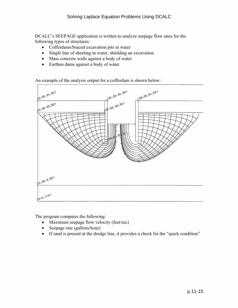
DCALC’s SEEPAGE application is written to analyze seepage flow rates for the following types of structures:

Cofferdams/braced excavation pits in water Single line of sheeting in water, shielding an excavation Mass concrete walls against a body of water Earthen dams against a body of water

An example of the analysis output for a cofferdam is shown below:

The program computes the following:

Maximum seepage flow velocity (feet/sec) Seepage rate (gallons/hour) If sand is present at the dredge line, it provides a check for the “quick condition”


p.11-16

11.6 Solving Torsional Properties Using the TORSION Application This program determines the torsional properties for any solid using the finite difference method. The resulting torsional stiffness property, “J”, is used in the following equation:

ϴ= T/(J*G) where

ϴ= angle of twist per unit length T = Torsion G= Modulus of elasticity in shear

Torsional properties were first determined by Saint- Venant in 1855. In 1903, Prandtl proposed a reformulation of the torsional problem which is based on a function, “ϕ”, called the stress function, with the following characteristics, τxz = ∂ϕ/∂y and τyz = -∂ϕ/∂x (Ref. 3, Eq. 149)

Saint-Venant (1797-1886)

Ludwig Prandtl (187501953)

Using the stress function, the torsional problem becomes a Poisson differential equation of the form,

∂2ϕ/∂x2 + ∂2ϕ/∂y2 = -2*G* ϴ (Ref. 3, Eq. 150) Boundary Conditions:

Along all exterior boundaries, set ϕ=0 Along all interior void boundaries, set the slope, ∂ϕ/∂n, so that the integral around

the void, ∑(∂ϕ/∂n)ds = -2*G* ϴ (Ref. 3, Appendix Eq. 30)

For equally spaced nodes, spaced a distance “h” apart, the following finite difference equation is applied to all interior nodes:

ϕi,j = ¼ (ϕi+1,j + ϕi-1,j + ϕi,j+1 + ϕi,j-1) + h2/4*(2*G) The torsional constant is computed as,

J = 2*∑ (ϕi,j) * h2 The solution for “J” is repeated many times, until the value stabilizes.


p.11-17

DCALC’s TORSION program was written to compute the torsion constant for any solid shape. An example of the output for a prestressed concrete bulb tee beam is shown below.

11.7 Summary: This paper has described several types of problems which involve the use of the Laplace equation and, similarly, the Poisson equation. Frequently Laplace/Poisson equations result from introducing a function (such as Airy stress function, velocity potential, stream function and vorticity) to solve a complex set of differential equations. A few of the methods of Computation Fluid Dynamics have been discussed as an iterative process for solving partial differential equations of this type. CFD programs using iterative techniques can be quite simple and short. However, the number of nodes used in CFD programs can be immense, requiring little storage space compared to the finite element method.


p.11-18

List of References: Reference 1: “Essential Computational Fluid Dynamics”, by Oleg Zikanov, published 2010 by John Wiley and Sons Reference 2: “Physical Behavior in Geotechnics”, by Fethi Azizi, first published 2007 by F. Azizi, School of Engineering, University of Plymouth ([email protected]) Reference 3:”Theory of Elasticity” by Timoshenko and Goodier Other References Used Reference 4: “Water Wave Mechanics For Engineers and Scientists”, by Robert Dean and Robert Dalrymple, copywrite 1991 by World Scientific Reference 5: “Engineering Design in Geotechnics”, by Fethi Aziz, first published 2007 by F. Azizi, School of Engineering, University of Plymouth ([email protected]) Reference 6: “Introduction to Fluid Mechanics”, by James John and William Haberman, copyright 1971, Prentice-Hall, Inc. Website Credits: For an excellent paper on how to compute solve Laplace equations, see “Finite Difference Method for the Solution of Laplace Equation”, by Ambar K. Mitra, Department of Aerospace Engineering, Iowa State University http://www.public.iastate.edu/~akmitra/aero361/design_web/Laplace.pdf For an excellent paper on computational fluid dynamics, see “Solution to two-dimensional Incompressible Navier-Stokes Equations with SIMPLE, SIMPLER and Vorticity-Stream Function Approaches”, by Maciej Matyka, Computational Physics Section of Theoretical Physics, University of Wroclaw in Poland ([email protected] http://panoramix.ift.uni.wroc.pl/~maq) Image Credits: Portraits of Laplace and Newton are from Wikipedia. Photos of Stokes and Prandtl are from Wikipedia Portrait of Saint-Venant is from “The MacTutor History of Mathematics Archive”, http://www-groups.dcs.st-and.ac.uk/~history/index.html

Solving Laplace Equation Problems Using DCALCdcalc.us/Tutorials/Chapter11.pdfStructural engineers...

Documents

Transcript of Solving Laplace Equation Problems Using DCALCdcalc.us/Tutorials/Chapter11.pdfStructural engineers...