Electrical Engineering department

Solving first order differential equations.And Finding a general solution to linear,constant coefficient differential equations.

1

WHAT IS MATLAB?

Matlab = Matrix Laboratory

A software environment for interactive numerical computations.

Examples:

Matrix computations and linear algebra

Solving nonlinear equations

Numerical solution of differential equations

Mathematical optimization

Statistics and data analysis

Signal processing

Simulation of engineering systems

2

MATLAB TOOLBOXES

MATLAB has a number of add-on software modules, called toolboxes, that perform more specialized computations.

Signal & Image ProcessingSignal Processing- Image Processing Communications - System Identification - Wavelet Filter Design

Control DesignControl System - Fuzzy Logic - Robust Control -µ-Analysis and Synthesis - LMI Control Model Predictive Control

More than 60 toolboxes!

3

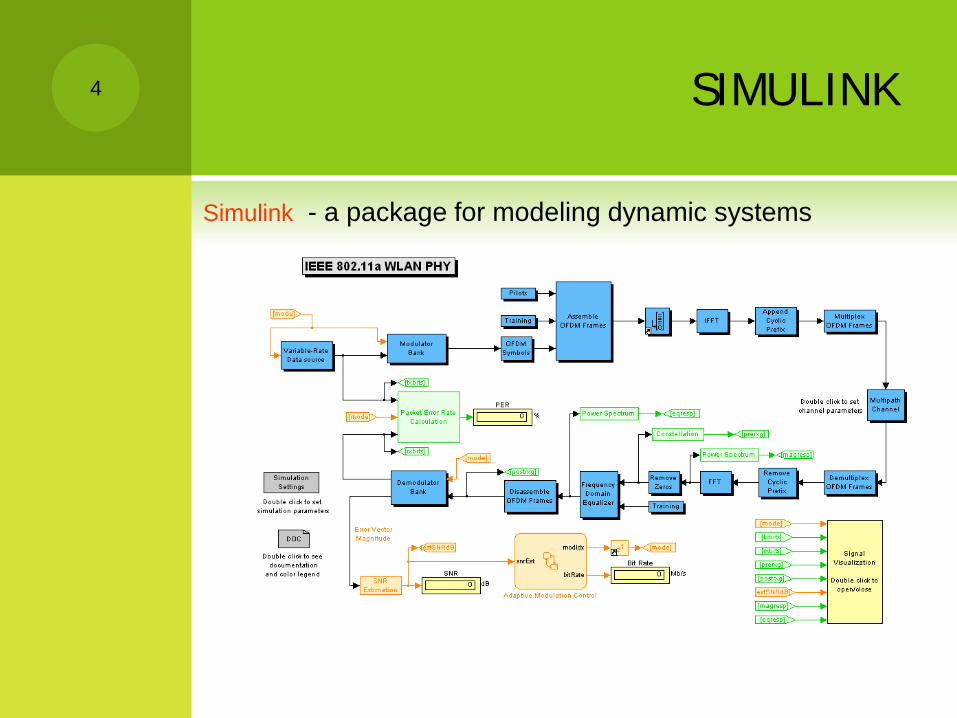
SIMULINK

Simulink - a package for modeling dynamic systems

4

MATLAB COMMAND

General

Help : help facility

Demo : run demonstrations

who : list variables in memory

what : list M-files on disk

Size : row and column dimensions

Length : vector length clear

Clear : workspace

exit : exit MATLAB quit same as exit

5

INTRODUCTION TODIFFERENTIAL EQUATIONS

Given independent variable t and dependent variabley(t), a linear ordinary differential equation withconstant coefficients is an equation of the form.

)()(... 01 tftyAdtdyA

dtydA n

n

n =+++

where A0, A1, …, An, are constants

6

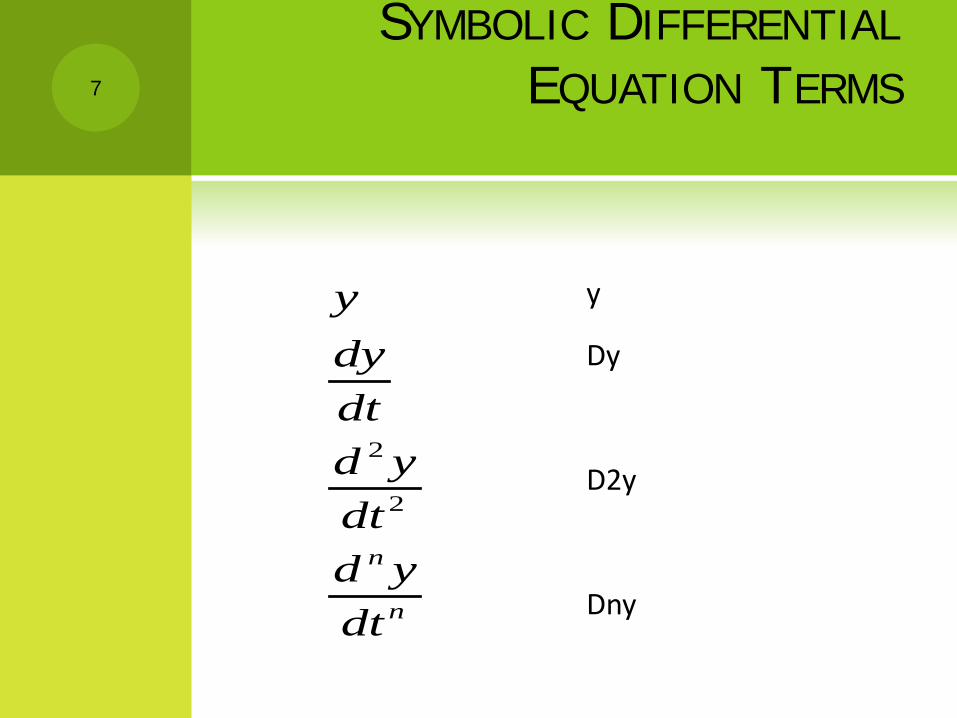
SYMBOLIC DIFFERENTIALEQUATION TERMS

2

2

n

n

ydydtd ydtd ydt

y

Dy

D2y

Dny

7

EXAMPLES

Examples of linear ordinary differential equation with constant coefficients:

2 12dy ydt

+ =

>> y = dsolve('Dy + 2*y = 12', 'y(0)=10')

y =

4*exp(-2*t) + 6

(0) 10y =

8

EXAMPLES

>> ezplot(y, [0 3])

Plot symbolic expression, equation, or function.

ezplot(f,[min,max]) plots f over the specified range. If f is a univariate expression or function, then [min,max]specifies the range for that variable.

By default, ezplot plots a univariate expression or function over the range [–2π 2π].

>> axis([0 3 0 10])

9

RESULT

0 0.5 1 1.5 2 2.5 30

1

2

3

4

5

6

7

8

9

10

t

4 exp(-2 t) + 6

10

EXAMPLE

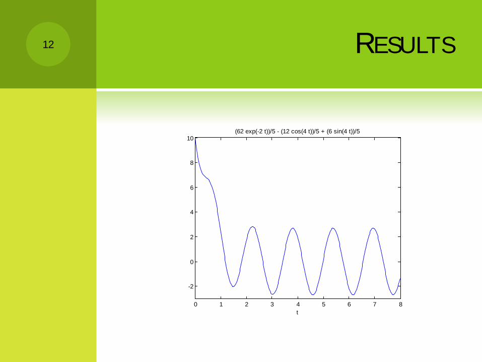
2 12sin 4dy y tdt

+ = (0) 10y =

>> y = dsolve('Dy + 2*y = 12*sin(4*t)', 'y(0)=10')

y =(62*exp(-2*t))/5 - (12*cos(4*t))/5 + (6*sin(4*t))/5

>> ezplot(y, [0 8])

>> axis([0 8 -3 10])

11

RESULTS

0 1 2 3 4 5 6 7 8

-2

0

2

4

6

8

10

t

(62 exp(-2 t))/5 - (12 cos(4 t))/5 + (6 sin(4 t))/5

12

EXAMPLE

2

2 3 2 24d y dy ydt dt

+ + =

(0) 10y = '(0) 0y =

>> y = dsolve('D2y + 3*Dy + 2*y = 24', 'y(0)=10', 'Dy(0)=0')

y =

2*exp(-2*t) - 4*exp(-t) + 12

>> ezplot(y, [0 5])

13

RESULT

0 0.5 1 1.5 2 2.5 3 3.5 4 4.5 5

10

10.2

10.4

10.6

10.8

11

11.2

11.4

11.6

11.8

12

t

2 exp(-2 t) - 4 exp(-t) + 12

14

EXAMPLE WITHOUT INITIALCONDITION

>> y = dsolve('Dy + 2*y = 12')

y = C14*exp(-2*t) + 6

The resulting solutions contain arbitrary constants C1, C2,....

2 12dy ydt

+ =

15

1ST-ORDER EQUATIONS (ODE45)

MATLAB has several numerical procedures for computing the solutions of first-order equations and systems of the form y’ = f(t, y);

Numerically approximate the solution of the first order differential equation.

The first step is to enter the equation by creating an “M-file” which contains the definition of your equation and is given a name for reference, such as “diffeqn”

The second step is to apply ode45 by using the syntax: [t, y] = ode45(‘diffeqn’, [t0,tf], y0)

16

1ST-ORDER EQUATIONS (ODE45)

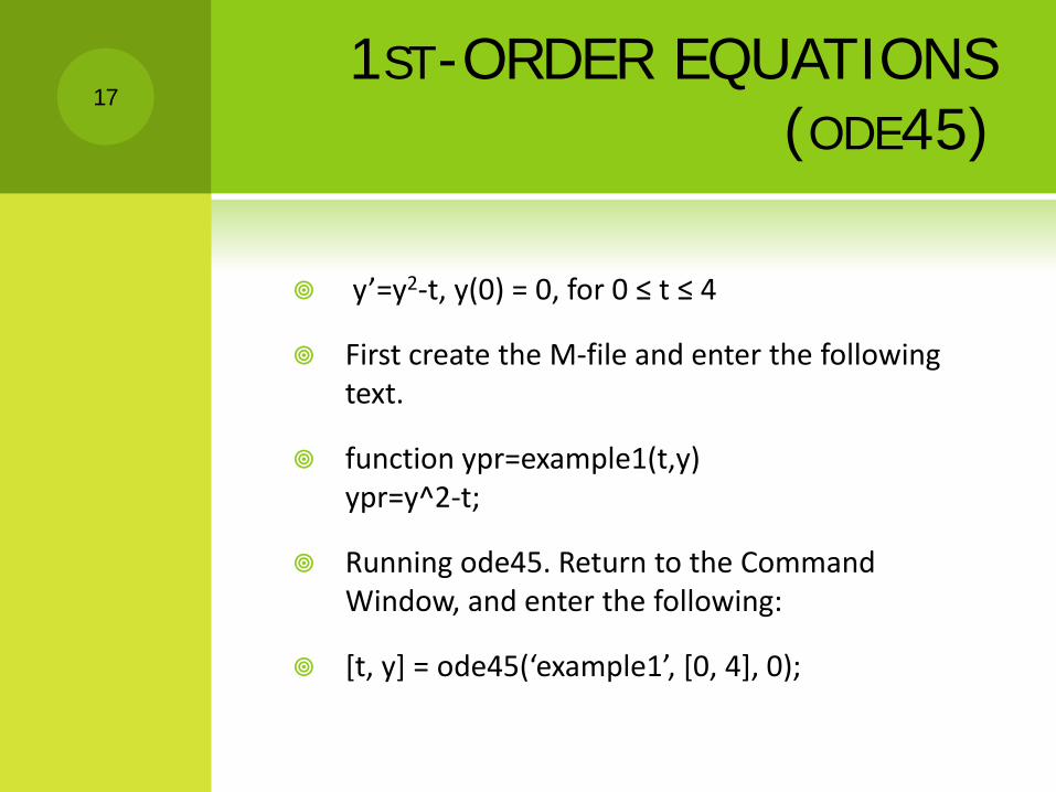
y’=y2-t, y(0) = 0, for 0 ≤ t ≤ 4

First create the M-file and enter the following text.

function ypr=example1(t,y) ypr=y^2-t;

Running ode45. Return to the Command Window, and enter the following:

[t, y] = ode45(‘example1’, [0, 4], 0);

17

RESULT

You can plot the solution y(t) by typing plot(t,y)

18