UNLV Theses, Dissertations, Professional Papers, and Capstones

December 2015

Solving differential equations with least square and collocation Solving differential equations with least square and collocation

methods methods

Katayoun Bodouhi Kazemi University of Nevada, Las Vegas

Follow this and additional works at: https://digitalscholarship.unlv.edu/thesesdissertations

Part of the Mathematics Commons

Repository Citation Repository Citation Kazemi, Katayoun Bodouhi, "Solving differential equations with least square and collocation methods" (2015). UNLV Theses, Dissertations, Professional Papers, and Capstones. 2548. http://dx.doi.org/10.34917/8220120

This Thesis is protected by copyright and/or related rights. It has been brought to you by Digital Scholarship@UNLV with permission from the rights-holder(s). You are free to use this Thesis in any way that is permitted by the copyright and related rights legislation that applies to your use. For other uses you need to obtain permission from the rights-holder(s) directly, unless additional rights are indicated by a Creative Commons license in the record and/or on the work itself. This Thesis has been accepted for inclusion in UNLV Theses, Dissertations, Professional Papers, and Capstones by an authorized administrator of Digital Scholarship@UNLV. For more information, please contact digitalscholarship@unlv.edu.

SOLVING DIFFERENTIAL EQUATIONS WITH LEAST SQUARE

AND COLLOCATION METHODS

by

Katayoun Bodouhi Kazemi

Master of Science in Engineering Management

George Washington University

2004

A thesis submitted in partial fulfillment

of the requirements for the

Master of Science-Mathematical Science

Department of Mathematical Sciences

College of Sciences

The Graduate College

University of Nevada, Las Vegas

December 2015

ii

Thesis Approval

The Graduate College

The University of Nevada, Las Vegas

July 9, 2015

This thesis prepared by

Katayoun Bodouhi Kazemi

entitled

Solving Differential Equations with Least Square and Collocation Methods

is approved in partial fulfillment of the requirements for the degree of

Master of Science –Mathematical Sciences

Department of Mathematical Sciences

Xin Li, Ph.D. Kathryn Hausbeck Korgan, Ph.D. Examination Committee Chair Graduate College Interim Dean

Zhonghai Ding, Ph.D. Examination Committee Member

Rohan Dalpatadu, Ph.D. Examination Committee Member

David Hatchett, Ph.D. Graduate College Faculty Representative

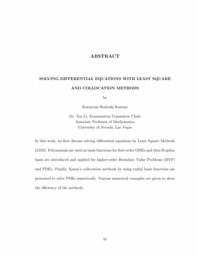
ABSTRACT

SOLVING DIFFERENTIAL EQUATIONS WITH LEAST SQUARE

AND COLLOCATION METHODS

by

Katayoun Bodouhi Kazemi

Dr. Xin Li, Examination Committee Chair

Associate Professor of Mathematics

University of Nevada, Las Vegas

In this work, we first discuss solving differential equations by Least Square Methods

(LSM). Polynomials are used as basis functions for first-order ODEs and then B-spline

basis are introduced and applied for higher-order Boundary Value Problems (BVP)

and PDEs. Finally, Kansa’s collocation methods by using radial basis functions are

presented to solve PDEs numerically. Various numerical examples are given to show

the efficiency of the methods.

iii

TABLE OF CONTENTS

ABSTRACT . . . . . . . . . . . . . . . . . . . . . . . . . . . . . . . . . . . . . . . . . . . . . . . . . . . . . . . . . . . . . . . . . . . . . iii

LIST OF FIGURES . . . . . . . . . . . . . . . . . . . . . . . . . . . . . . . . . . . . . . . . . . . . . . . . . . . . . . . . . . . . . . vi

LIST OF TABLES . . . . . . . . . . . . . . . . . . . . . . . . . . . . . . . . . . . . . . . . . . . . . . . . . . . . . . . . . . . . . . . vii

ACKNOWLEDGEMENTS . . . . . . . . . . . . . . . . . . . . . . . . . . . . . . . . . . . . . . . . . . . . . . . . . . . . . . . viii

1 - INTRODUCTION TO LEAST SQUARE METHODS 11.1. Example of using LSM to solve a first-order ODE . . . . . . . . . . . 4

1.1.1. Continuous Least Square Method . . . . . . . . . . . . . . . . 41.1.2. Discrete Least Square Methods . . . . . . . . . . . . . . . . . 8

1.2. Example of using LSM to solve a second-order ODE . . . . . . . . . . 10

2 - LEAST SQUARE METHODS BY B-SPLINES 122.1. B-spline Basis Functions . . . . . . . . . . . . . . . . . . . . . . . . . 122.2. Computing B-spline basis functions . . . . . . . . . . . . . . . . . . . 132.3. Solving a 2nd-order ODE by B-splines . . . . . . . . . . . . . . . . . 182.4. More examples of solving higher order ODEs . . . . . . . . . . . . . . 222.5. Solving a PDE by B-spline basis . . . . . . . . . . . . . . . . . . . . 29

3 - DIFFERENTIAL MODELING IN APPLICATIONS 323.1. Mass spring system . . . . . . . . . . . . . . . . . . . . . . . . . . . . 323.2. Wave modeling . . . . . . . . . . . . . . . . . . . . . . . . . . . . . . 343.3. Diffusion equation . . . . . . . . . . . . . . . . . . . . . . . . . . . . . 37

4 - COLLOCATION METHODS BY RADIAL BASIS FUNCTIONS 394.1. Radial Basis Functions . . . . . . . . . . . . . . . . . . . . . . . . . . 394.2. Kansa collocation methods . . . . . . . . . . . . . . . . . . . . . . . . 414.3. Solving PDEs by RBFs . . . . . . . . . . . . . . . . . . . . . . . . . . 464.4. Conclusion . . . . . . . . . . . . . . . . . . . . . . . . . . . . . . . . . 52

REFERENCES . . . . . . . . . . . . . . . . . . . . . . . . . . . . . . . . . . . . . . . . . . . . . . . . . . . . . . . . . . . . . . . . . . 54

iv

v

LIST OF FIGURES

1.1 Exact solution, approximate solution, and the error for first order ODEexample when N=3 . . . . . . . . . . . . . . . . . . . . . . . . . . . 6

1.2 Exact solution, approximate solution, and the error for first order ODEexample when N=5 . . . . . . . . . . . . . . . . . . . . . . . . . . . . 8

1.3 Solution of an example of first order ODE by discrete Least SquareMathod with N=3 and 3 points in the domain and on the boundary . 9

1.4 Solution of an example of first order ODE by discrete Least SquareMathod with N=3 and 5 points in the domain and boundary . . . . . 10

1.5 Solution and error for example of second order ODE by LSM . . . . . 11

2.1 Graph of Ni,0(u) for knots 0, 1, 2, 3 . . . . . . . . . . . . . . . . . . . 132.2 Triangular computation scheme for Ni,k(u) . . . . . . . . . . . . . . . 142.3 Graph of Ni,1(u) for knots 0, 1, 2, 3 . . . . . . . . . . . . . . . . . . . 152.4 Graph of Ni,2(u) for knots 0, 1, 2, 3 . . . . . . . . . . . . . . . . . . . 162.5 Graph of Ni,3(u) for knots 0, 1, 2, 3 . . . . . . . . . . . . . . . . . . . 172.6 Graph of Ni,4(u) for knots 0, 1, 2, 3 . . . . . . . . . . . . . . . . . . . 172.7 Solving a second order ODE by LSM using B-spline basis when k=1 . 212.8 Solving a third order ODE by discerete LSM using B-spline basis when

k=0 . . . . . . . . . . . . . . . . . . . . . . . . . . . . . . . . . . . . 242.9 Solving third order ODE by discerete LSM using B-spline basis when

k=1 . . . . . . . . . . . . . . . . . . . . . . . . . . . . . . . . . . . . 252.10 Solving a six-order ODE by LSM using B-spline basis when k=1 . . . 28

3.1 Figure for the system . . . . . . . . . . . . . . . . . . . . . . . . . . . 333.2 x approximate vs t and error for mass spring sysytem . . . . . . . . . 343.3 Initial position of the bird on the wire . . . . . . . . . . . . . . . . . 363.4 Approximate and exact concentration distribution of medicine and er-

ror at 80 sec . . . . . . . . . . . . . . . . . . . . . . . . . . . . . . . 38

4.1 Gaussian radial basis: left is centered at (10,10) with c=5, middle iscentered at (20,20) with c=3, right is centered at (30,30) with c=1 . 40

4.2 100 uniform points . . . . . . . . . . . . . . . . . . . . . . . . . . . . 424.3 100 Halton points . . . . . . . . . . . . . . . . . . . . . . . . . . . . . 424.4 100 Fence points . . . . . . . . . . . . . . . . . . . . . . . . . . . . . 434.5 100 Random points . . . . . . . . . . . . . . . . . . . . . . . . . . . . 434.6 Error for example of Poisson’s equation with 100 uniform collocation

points by Gaussian RBF . . . . . . . . . . . . . . . . . . . . . . . . . 474.7 Error for example of Poisson’s equation with 100 Halton collocation

points by Gaussian RBF . . . . . . . . . . . . . . . . . . . . . . . . . 47

vi

4.8 Error of an example of Poisson’s equation with Neumann boundarycondition with IMQ RBF (c = 3) (using 100 Halton collocation points) 49

4.9 Error of an example of Poisson’s equation with Neumann boundarycondition with IMQ RBF (c = 10) (using 100 Halton collocation points) 49

4.10 Error of an example of Elliptic equation with variable coefficient withIMQ RBF (c = 3) (using 100 uniform collocation points) . . . . . . . 51

4.11 Error of an example of PDE with mixed boundary conditions by IMQRBF (c = 3) (using 100 uniform collocation points) . . . . . . . . . . 52

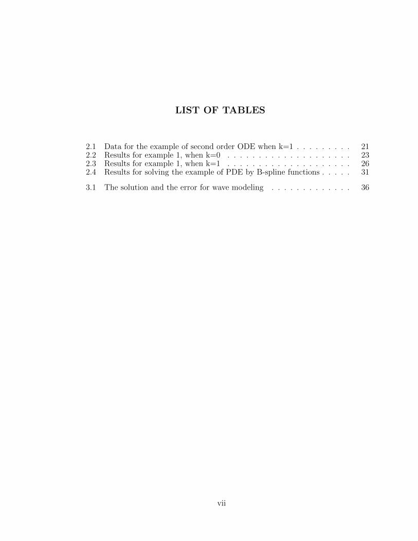
LIST OF TABLES

2.1 Data for the example of second order ODE when k=1 . . . . . . . . . 212.2 Results for example 1, when k=0 . . . . . . . . . . . . . . . . . . . . 232.3 Results for example 1, when k=1 . . . . . . . . . . . . . . . . . . . . 262.4 Results for solving the example of PDE by B-spline functions . . . . . 31

3.1 The solution and the error for wave modeling . . . . . . . . . . . . . 36

vii

ACKNOWLEDGEMENTS

I would like to thank Dr. Xin Li, for all his advice and help through out working on

this project. I extend my gratitude to Dr. Dalpatadu, Dr. Ding and Dr. Hattchet

for accepting to be in my committee and reviewing my work. My special thank

to my mom, my husband and my brother for their continuous support and help.

Finishing up my course work and working on this thesis were impossible without

their encouragements and supports. I dedicate this work to my late father, my mom,

my husband and my two little angels, Lilia and Alyssa.

viii

CHAPTER 1 - INTRODUCTION TO LEAST SQUARE

METHODS

Least Square Methods (LSM) have been used to solve differential equations in Finite

Element Methods (FEM). For description, we consider the following linear boundary

value problem [1]

L(y) = f(x) for x ∈ domain Ω,

W (y) = g(x) for x ∈ boundary ∂Ω,

where Ω is a domain in R1 or R2 or R3, L is differential operator, and W is the

boundary operator. When solving a differential equation by Finite Element Methods

(FEM), the solution is given by a sum of weighted basis functions. Using φi(x),

1 ≤ i ≤ N , for basis functions, an approximate solution is expressed as

y =N∑i=1

qiφi(x), (1.1)

where qi’s are coefficients (weights) and they can be determined by least square meth-

ods, explained below. To be precise, define the residual RL(x), RW (x) as follows

1

RL(x, y) = L(y)− f(x) for x ∈ domain Ω,

RW (x, y) = W (y)− g(x) for x ∈ boundary ∂Ω.

Use yexact for exact solution of the boundary value problem. Then, it is obvious that

RL(x, yexact) = 0 and RW (x, yexact) = 0.

In using LSM, the goal is to find the coefficients qi’s by minimizing the error function

in L2 norm, defined by

E =

∫Ω

R2L(x, y)dx +

∫∂Ω

R2W (x, y)dx.

The best approximate solution is determined by finding the minimal value of E, or

∂E

∂qi= 0, for i = 1, .., N,

which yields

∫Ω

RL(x, y)∂RL

∂qidx +

∫∂Ω

RW (x, y)∂RW

∂qidx = 0, i = 1, .., N.

The above formulation is in continuous format and the squared residuals are inte-

grated over the domain. This will give N linear equations and by some algebraic

manipulation can be written as:

Da = b,

2

where D is an N ×N matrix, a = [q1, q2, ..., qN ]T , and some column vector b.

The following format is the discrete formulation and the squared residuals are summed

at finite points xi, 1 ≤ i ≤ k, in domain, and xi, k + 1 ≤ i ≤ m, on the boundary

points. Define

E =k∑i=1

R2L(xi, y) +

m∑i=k+1

R2W (xi, y).

Write

r =

RL(a,x1)

.

.

RL(a,xk)

RW (a,xk+1)

.

.

RW (a,xm)

=

Ly(a,x1)− f(x1)

.

.

Ly(a,xk)− f(xk)

Ly(a,xk+1)− f(xk+1)

.

.

Ly(a,xm)− f(xm)

.

The discrete least square solution, which minimizes E = rT r, is then determined by

∂E

∂qi= 0, for i = 1, .., N.

Choosing the right basis function φi is very important in LSM. In linear ODE we

usually use polynomials. In the next section, polynomials with different degrees are

used and compared to solve some first order ODE and second order ODEs in both

3

continuous and discrete formats.

1.1. Example of using LSM to solve a first-order ODE

1.1.1. Continuous Least Square Method

First, we want to solve an example of a first order ordinary differential equation

as an illustration to present least squares methods. Assume that we have the following

initial value problem of the first order ODE:

dy

dx− y = 0, y(0) = 1,

where 0 ≤ x ≤ 1.

Let

L(x, y) =dy

dx− y

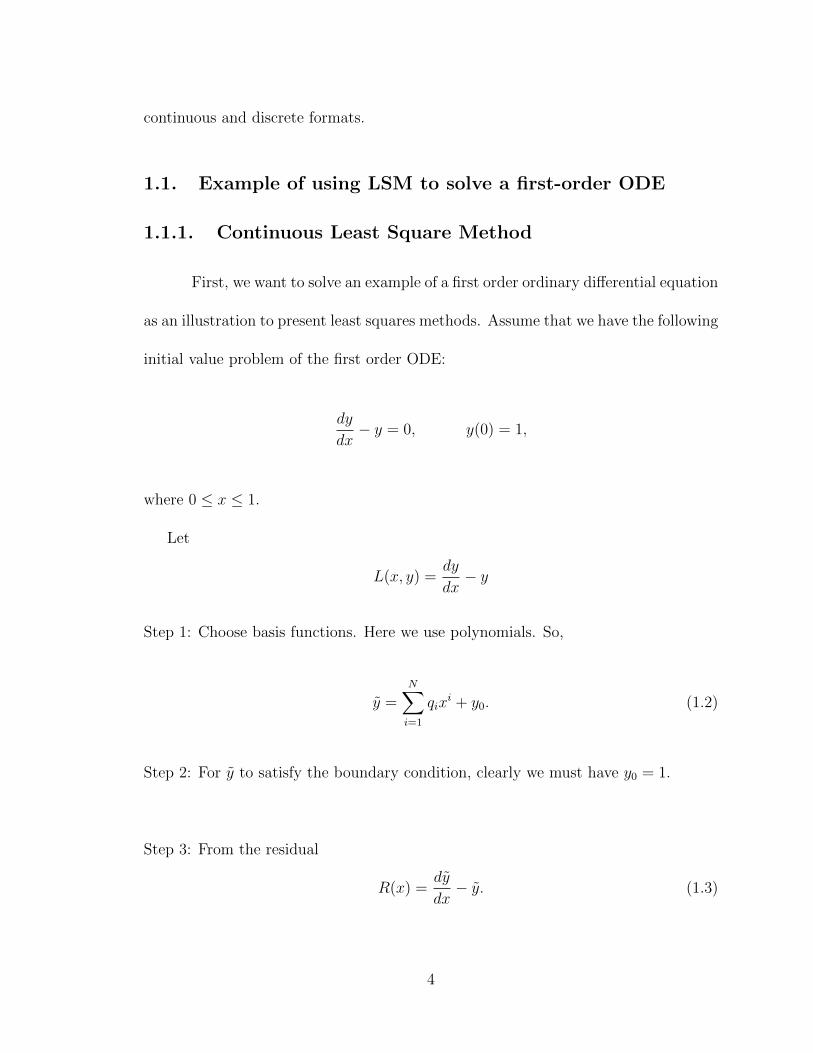
Step 1: Choose basis functions. Here we use polynomials. So,

y =N∑i=1

qixi + y0. (1.2)

Step 2: For y to satisfy the boundary condition, clearly we must have y0 = 1.

Step 3: From the residual

R(x) =dy

dx− y. (1.3)

4

By replacing y(x) from (1.2) into (1.3), we will get:

R(x) =d(∑N

i=1 qixi + 1)

dx− (

N∑i=1

qixi + 1).

Step 4: To minimize the square error, we need to set up

E =

∫ 1

0

R2(x)dx.

The best approximate solution is determined by finding the minimal value of E, or

∂E

∂qi= 0, for i = 1, .., N

∫ 1

0

R(x)∂R

∂qidx = 0, i = 1, .., N

or

(R(x),

∂R(x)

∂qi

)= 0 for i = 1, 2, 3, ........, N

These lead to a linear system which can be solved for qi’s.

The above equations were solved by a Matlab program. The following results were

obtained by running the code for different N ’s.

5

When N=3, we get the following matrices

D =

0.33 0.25 0.2

0.25 0.533 0.66

0.2 0.66 0.94

, b =

−0.5

−0.66

−0.75

, a =

q1

q2

q3

,

and the approximate solution is

y = 0.2797x3 + 0.4255x2 + 1.0131x+ 1.

Results are shown in the figure 1.1.

0 0.1 0.2 0.3 0.4 0.5 0.6 0.7 0.8 0.9 11

1.5

2

2.5

3

x

y

x vs y approximate and y exact when N=3

y approximate

y exact

0 0.1 0.2 0.3 0.4 0.5 0.6 0.7 0.8 0.9 1−1

−0.5

0

0.5

1x 10

−3

x

Err

or

x vs error

Figure 1.1: Exact solution, approximate solution, and the error for first order ODEexample when N=3

6

When N=5, We get the following matrices

D =

0.33 0.25 0.2 0.16 0.14

0.25 0.533 0.66 0.74 0.79

0.2 0.66 0.94 1.125 1.25

0.16 0.74 0.125 1.125 1.6

0.14 0.79 1.125 1.6 1.86

, b =

−0.5

−0.66

−0.75

−0.8

−0.83

, a =

q1

q2

q3

q4

q5

.

The approximate solution is

y = 0.0139x5 + 0.0349x4 + 0.1702x3 + 0.4992x2 + 1.0001x+ 1.

We know that the exact solution is

yexact = ex.

The following figures show the graph of approximate and exact solutions and the

errors. The error is defined as

error = yexact − y.

7

0 0.1 0.2 0.3 0.4 0.5 0.6 0.7 0.8 0.9 11

1.5

2

2.5

3

x

y

x vs y approximate and y exact when N=5

y approximate

y exact

0 0.1 0.2 0.3 0.4 0.5 0.6 0.7 0.8 0.9 1−2

−1

0

1

2x 10

−6

x

Err

or

x vs error

Figure 1.2: Exact solution, approximate solution, and the error for first order ODEexample when N=5

1.1.2. Discrete Least Square Methods

For the above example we can solve the first order ODE by least square method

in a discrete form. To approach the problem in a discrete method, we approximate

the solution in discrete points within the domain and on the boundary points.

When N = 3, three discrete points x1 = 0, x2 = 0.5 and x3 = 1 were chosen. Matrices

r and E were similarly made. Then set

∂E

∂qi= 0 for i = 1, 2, 3.

qi’s are calculated. The approximate solution is

y =2

3x3 +

3

7x2 + x+ 1.

8

Figure 1.3 shows the graph of the approximate solution and exact solution as well as

the error.

0 0.1 0.2 0.3 0.4 0.5 0.6 0.7 0.8 0.9 11

1.5

2

2.5

3

x

y d

iscre

te

x vs y ,3 discrete points in the domain

0 0.1 0.2 0.3 0.4 0.5 0.6 0.7 0.8 0.9 10

1

2

3

4

5

6x 10

−3

x

Err

or

x vs error

Figure 1.3: Solution of an example of first order ODE by discrete Least SquareMathod with N=3 and 3 points in the domain and on the boundary

When N = 5, 5 discrete points x1 = 0.2, x2 = 0.4, x3 = 0.6, x4 = 0.8 and x5 = 1

were chosen. By following the exact steps as above, we have

y = 0.2817x3 + 0.4288x2 + 1.006x+ 1.

Figure 1.4 shows the graph of the approximate solution and exact solution as well as

the error.

9

0 0.1 0.2 0.3 0.4 0.5 0.6 0.7 0.8 0.9 1−2

−1

0

1

2x 10

−6

x

err

or

x vs error continuous

0 0.1 0.2 0.3 0.4 0.5 0.6 0.7 0.8 0.9 10

2

4x 10

−3

xE

rror

x vs error discrete

0 0.1 0.2 0.3 0.4 0.5 0.6 0.7 0.8 0.9 11

2

3

x

y

x vs y discrete

y discrete

y exact

Figure 1.4: Solution of an example of first order ODE by discrete Least SquareMathod with N=3 and 5 points in the domain and boundary

1.2. Example of using LSM to solve a second-order ODE

Now consider the following second order ODE:

dy2

dx2+dy

dx+ 4y = 4x2 + 10x+ 2, (1.4)

with Boundary conditions

y(0) = 1 and y′(0) = 2.

The exact solution is

y(x) = 2 exp(−x)− exp(−4x) + x2.

10

Now,we use polynomials as basis functions, so the approximate solution will be in the

form of

y =N∑i=1

qiφi + y0. (1.5)

To satisfy the boundary conditions, we need to have y0 = 1 and q1 = 2. By following

LSM and solving the systems of equations in Matlab, we will get the solution and

error below (Figure 1.5). As we saw, polynomials give us acceptable errors as basis

Figure 1.5: Solution and error for example of second order ODE by LSM

functions when we use them in least square method for first order ODEs in both

discrete and continuous cases. However, they do not give errors in acceptable range

when solving second order ODEs and PDEs. In the next chapter, we introduce B-

spline basis functions which satisfy our need.

11

CHAPTER 2 - LEAST SQUARE METHODS BY

B-SPLINES

In this chapter, we will introduce and use B-spline basis functions for solving ODE’s

and PDE’s by LSM.

2.1. B-spline Basis Functions

To introduce B-splines, let U be a set of n+ 1 non-decreasing numbers, u0 ≤ u1 ≤

... ≤ un, which are called knots, and the half-open interval [ui, ui+1) is the ith knot

span for 0 ≤ i ≤ n − 1. The knots can be spaced uniformly or non-uniformly. They

also can appear multiple times and in that case they are called multiple knots.

For ui < ui+1, the ith B-spline of degree 0 is defined by

Ni,0(u) =

1, ui ≤ u < ui+1,

0, otherwise,

and for k ≥ 1,

Ni,k(u) =u− uiui+k − ui

Ni,k−1(u) +ui+k+1 − uui+k+1 − ui+1

Ni+1,k−1(u).

12

The above formula is usually referred to as Cox-de Boor recursion formula.

It is obvious that for k = 0 the basis functions are all step functions. This is because

the basis function Ni,0(u) is 1 if u is in the ith knot span [ui, ui+1). For example, for

knots u0 = 0, u1 = 1, u2 = 2 and u3 = 3 the knot spans are [0, 1), [1, 2), [2, 3). The

basis function of degree 0 are N0,0(u) = 1 on [0, 1) and 0 elsewhere, N1,0(u) = 1 on

[1, 2) and 0 elsewhere, N2,0 = 1 on [2, 3) and 0 elsewhere (Figure 2.1).

Figure 2.1: Graph of Ni,0(u) for knots 0, 1, 2, 3

Figure 2.2 shows how we can compute Ni,k(u) using the triangular computation

scheme .

2.2. Computing B-spline basis functions

As an example let’s compute the basis functions for k=1. Choose the following

knots [2]

u0 = 0, u1 = 1, u2 = 2, u3 = 3.

13

Figure 2.2: Triangular computation scheme for Ni,k(u)

Then, by definition above,

N0,1(u) =u− u0

u1 − u0

N0,0(u) +u2 − xu2 − u1

N1,0(u),

by replacing the values of the knots we will get

N0,1(u) = uN0,0(x) + (2− u)N1,0(u).

If u is in [0, 1), then N0,0 = 1 and N1,0 = 0. Therefore, N0,1(U) = u. If u is in [1, 2),

then N0,0 = 0 and N1,0 = 1. Therefore, N0,1(U) = 2− u.

14

Similarly, N1,1(u) = u− 1, if u is in [1, 2) and N1,1(u) = 3− u, if u is in [2, 3). Figure

2.3 shows the graph of Ni,1(x).

Figure 2.3: Graph of Ni,1(u) for knots 0, 1, 2, 3

Now,

N0,2(u) =u− u0

u2 − u0

N0,1(u) +u3 − uu3 − u1

N1,1(u)

If 0 ≤ u < 1, then, only N0,1(u) = u contributes to N0,2(u), and

N0,2(u) = 0.5u2.

For 1 ≤ u < 2 both N0,1(u) = 2 − u and N1,1(u) = u − 1 contribute to N0,2(u). In

this case,

N0,2(u) = (0.5u)(2− u) + 0.5(3− u)(3− u) = 0.5(−3 + 6u− 2u2).

15

Finally, if 2 ≤ x < 3, only N1,1(u) = 3− u contributes to N0,2(u),

N0,2(u) = (0.5)(3− u)(3− u) = 0.5(3− u)2

Figure 2.4 shows the graph of Ni,2(u). It is clear that the curve segments join at the

knots and here the graph is smooth. In general, if there are multiple knots, the graph

is not smooth.

Figure 2.4: Graph of Ni,2(u) for knots 0, 1, 2, 3

Following triangular scheme in Figure 2.2, we are able to compute all Ni,k(u)s in

different knot span. Figures 2.5 and 2.6 show the graphs of Ni,3(u) and Ni,4(u) in

different knot spans.

16

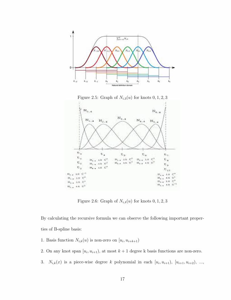
Figure 2.5: Graph of Ni,3(u) for knots 0, 1, 2, 3

Figure 2.6: Graph of Ni,4(u) for knots 0, 1, 2, 3

By calculating the recursive formula we can observe the following important proper-

ties of B-spline basis:

1. Basis function Ni,k(u) is non-zero on [ui, ui+k+1)

2. On any knot span [ui, ui+1), at most k + 1 degree k basis functions are non-zero.

3. Ni,k(x) is a piece-wise degree k polynomial in each [ui, ui+1), [ui+1, ui+2), ...,

17

[ui+k, ui+k+1) .

4. For all i, k and u, Ni,k(u) is non-negative.

5. Ni,k(u) is locally supported. Namely, Ni,k(u) is a non-zero piece-wise polynomial

on [ui, ui+k+1).

6. The sum of all non-zero degree k basis functions on span [ui, ui+1) is 1.

7. If ui is a knot of multiplicity m, then Ni,k(u) is Ck−m continuous at ui.

2.3. Solving a 2nd-order ODE by B-splines

In the previous chapter, we saw that polynomials are not suitable to be used as

basis functions in LSM for solving 2nd order ODEs. Here, we want to show that

B-splines give us an acceptable approximate solution by LSM. As we saw, if the

knots ui are distinct or of multiplicity 1, B-spline basis functions of degree k are Ck−1

continuous. This property is helpful when we use B-spline functions as the basis in

Least Square method.

To get a set of basis functions in LSM, as in the paper by Loghmani [3], we use

translations and dialations of the standard B-spline functions. To be precise, for an

interval [a, b], we consider equal partitions

a < a+ h < a+ 2h < ... < a+ 3 · 2kh = b,

18

where h = b−a3·2k .

Define

Bki(t) = B

(3 · 2k

b− a(t− a)− i

), (i = −3,−2,−1, ..., 3 · 2k − 1)

where B is a B-spline and Bki with k ∈ N, (i = −3,−2, ..., 3 · 2k − 1) is translation

and dilation of B.

Example: We now consider the following 2nd-order ODE

dy2

dx2+dy

dx+ 4y = 4x2 + 10x+ 2 (2.1)

with the boundary condition

y(0) = 1 and y′(0) = 2.

The exact solution is

y(x) = 2 exp(−x)− exp(−4x) + x2.

Since we have a second order ODE, we use the quadratic B-spline basis function.

B(t) =

t2, 0 ≤ t ≤ 1,

−2t2 + 6t− 3, 1 ≤ t ≤ 2,

(3− t)2, 2 ≤ t ≤ 3,

0, otherwise.

19

Choose k = 1, so h = 16

and the partitions will be

0 ≤ 1

6≤ 1

3≤ 1

2≤ 2

3≤ 5

6≤ 1.

Define the approximate solution as

y =5∑

i=−2

ciB1i(x).

Set the residual as

r =d2y

dx2+dy

dx+ 4y − 4x2 − 10x− 2,

or

r =d2(∑5

i=−2 ciB1i(x))

dx2+d(∑5

i=−2 ciB1i(x))

dx+ 4(

5∑i=−2

ciB1i(x))− 4x2 − 10x− 2.

To satisfy the boundary conditions we need to have c−1 = 712

and c−2 = 512.

We use LSM at discrete points x0 = 0, x1 = 112

, x2 = 14, x3 = 5

12, x4 = 7

12, x5 = 3

4,

x6 = 1112

, x7 = 1. Then we solve the system of equations in Matlab to find ci’s. The

results are given in Figure 2.7 and Table 2.1.

As it can be seen, the error is within acceptable range and B-spline basis is a much

better choice than polynomials.

20

Figure 2.7: Solving a second order ODE by LSM using B-spline basis when k=1

x y exact y approximate0 1 1

0.08 1.1305 1.12970.25 1.2522 1.24660.42 1.3032 1.30910.58 1.3594 1.36050.75 1.4574 1.45550.92 1.6144 1.6108

1 1.7174 1.7134

Table 2.1: Data for the example of second order ODE when k=1

21

2.4. More examples of solving higher order ODEs

Example 1: Now consider the following BVP

y′′′(x) = y(x)− 3ex, 0 < x < 1,

y′(0) = 0, y(1) = 0, y(0) = 1.

The exact solution is y(x) = (1 − x)ex [5]. For this problem we want to use the

following cubic B-spline as the basis function

B(t) =

t3, 0 ≤ t ≤ 1,

−3t3 + 12t2 − 12t+ 4, 1 ≤ t ≤ 2,

3t3 − 24t2 + 60t− 44, 2 ≤ t ≤ 3,

(4− t)3, 3 ≤ t ≤ 4,

0, otherwise.

Choose k = 0, then h = 13

and consider the following partitions

0 ≤ 1

3≤ 2

3≤ 1.

Define the approximate solution as

y =2∑

i=−3

ciB0i(x).

22

Define the residual as

r =d3y

dx3− y + 3ex,

or

r =d3(∑2

i=−3 ciB0i(x))

dx3−

2∑i=−3

ciB0i(x)) + 3ex.

To satisfy the boundary condition we need to have

c−3 = c−1, c−2 = −0.5c−1 +1

4, c0 = −4c1 − c2.

We follow least square method calculated at the following discrete points,

x1 = 0, x2 =1

9, x3 =

2

9, x4 =

1

3, x5 =

4

9, x6 =

5

9, x7 =

2

3, x8 =

7

9, x9 =

8

9, x10 = 1.

By solving the systems of equations in Matlab we will get the following results (Table

2.2 and Figure 2.8).

x y approximate y exact0 1 10.1111 0.993 0.99330.2222 0.9701 0.97130.3333 0.9281 0.93040.4444 0.8631 0.86650.5555 0.7705 0.77450.6666 0.6449 0.64920.7777 0.4803 0.48370.8888 0.2682 0.27021 0 0

Table 2.2: Results for example 1, when k=0

23

Figure 2.8: Solving a third order ODE by discerete LSM using B-spline basis whenk=0

Now, if k = 1, then h = 16

and consider the following partitions:

0 ≤ 1

6≤ 1

3≤ 1

2≤ 2

3≤ 5

6≤ 1

We follow discrete LSM at the following discrete points:

x1 = 0, x2 =1

12, x3 =

1

4, x4 =

5

12, x5 =

4

9, x6 =

5

9, x7 =

7

12, x8 =

3

4, x9 =

11

12, x10 = 1.

24

. After solving the system of equations in Matlab for ci’s, we will get the following

results (Figure 2.9 and Table 2.3).

Figure 2.9: Solving third order ODE by discerete LSM using B-spline basis when k=1

The results show that even for k = 0, the error is within acceptable range. As

we increase k the error becomes smaller.

25

x y approximate y exact error0 1 1 5.551E-178.33E-2 0.9962 0.9962 -3.762E-50.25 0.9628 0.9629 -1.7359E-40.4166 0.8846 0.8849 -1.8709E-40.5833 0.746 0.7467 -9.377E-50.75 0.529 0.5292 7.1409E-50.9166 0.2086 0.2084 2.2269E-41 6.9388E-18 0 6.9389E-18

Table 2.3: Results for example 1, when k=1

Example 2: Consider a sixth degree linear boundary value problem [6]

y(6) + xy = −(24 + 11x+ x3)e3, 0 ≤ x ≤ 1

subject to

y(0) = 0, y(1) = 0,

y′(0) = 1, y′(1) = −e,

y′′(0) = 0, y′′(1) = −4e.

The exact solution of the above problem is

y(x) = x(1− x)ex.

Now, we want to solve this problem with LSM using B-spline basis function. Logh-

26

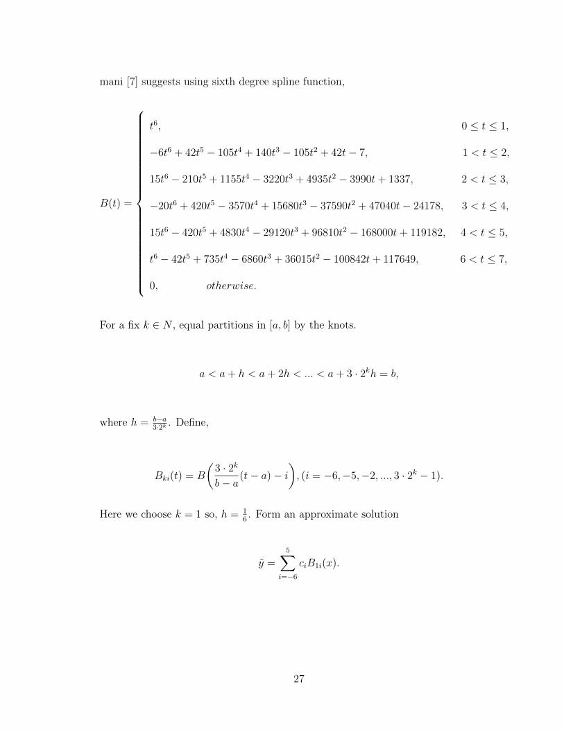
mani [7] suggests using sixth degree spline function,

B(t) =

t6, 0 ≤ t ≤ 1,

−6t6 + 42t5 − 105t4 + 140t3 − 105t2 + 42t− 7, 1 < t ≤ 2,

15t6 − 210t5 + 1155t4 − 3220t3 + 4935t2 − 3990t+ 1337, 2 < t ≤ 3,

−20t6 + 420t5 − 3570t4 + 15680t3 − 37590t2 + 47040t− 24178, 3 < t ≤ 4,

15t6 − 420t5 + 4830t4 − 29120t3 + 96810t2 − 168000t+ 119182, 4 < t ≤ 5,

t6 − 42t5 + 735t4 − 6860t3 + 36015t2 − 100842t+ 117649, 6 < t ≤ 7,

0, otherwise.

For a fix k ∈ N , equal partitions in [a, b] by the knots.

a < a+ h < a+ 2h < ... < a+ 3 · 2kh = b,

where h = b−a3·2k . Define,

Bki(t) = B

(3 · 2k

b− a(t− a)− i

), (i = −6,−5,−2, ..., 3 · 2k − 1).

Here we choose k = 1 so, h = 16. Form an approximate solution

y =5∑

i=−6

ciB1i(x).

27

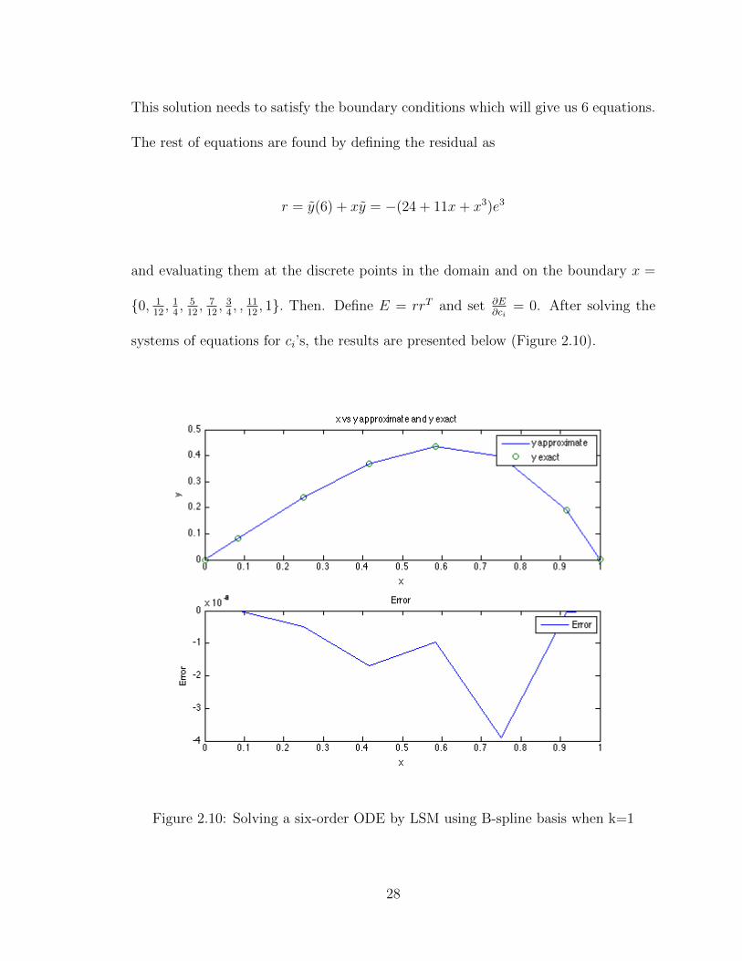
This solution needs to satisfy the boundary conditions which will give us 6 equations.

The rest of equations are found by defining the residual as

r = y(6) + xy = −(24 + 11x+ x3)e3

and evaluating them at the discrete points in the domain and on the boundary x =

0, 112, 1

4, 5

12, 7

12, 3

4, , 11

12, 1. Then. Define E = rrT and set ∂E

∂ci= 0. After solving the

systems of equations for ci’s, the results are presented below (Figure 2.10).

Figure 2.10: Solving a six-order ODE by LSM using B-spline basis when k=1

28

2.5. Solving a PDE by B-spline basis

Consider the following Poisson’s equation

∂2u

∂x2+∂2u

∂y2= 6xy(1− y)− 2x3

for 0 ≤ x ≤ 1 and 0 ≤ y ≤ 1. Suppose that u(x, y) satisfies mixed boundary

conditions

u(0, y) = 0,

u(1, y) = y(1− y),

u(x, 0) = u(x, 1) = 0,

Choose k = 0, then h = 13

and consider the following partitions 0 ≤ 13≤ 2

3≤ 1 on

both x and y axes. Now define the following approximate solution by LSM

u(x, y) =2∑

i=−3

(2∑

j=−3

cijB0i(x)B0j(y)),

where B0i and B0j are dilations and translations of the cubic B-spline.

cij, i = −3,−2, ....1, 2 and j = −3,−2, ....1, 2 are the coefficients to be found in

LSM. u(x, y) needs to satisfy the boundary points, which gives us 12 equations for 12

discrete points on the boundary.

29

Now, define the residual as

r(x, y) =∂2u

∂x2+∂2u

∂y2− 6xy(1− y)− 2x3.

Follow the discrete LSM explained in the earlier chapter to construct E =∑r2. The

sum is over 49 uniform discrete points in the domain.

By LSM we need to have

∂E

∂ci,j= 0, for i = −3,−2, ....1, 2 and j = −3,−2, ....1, 2

The 36 unknown cij will be found by the above equations and equations from bound-

ary conditions.

The table below shows the exact and approximate solution for discrete points (Table

2.4).

30

x y u exact u approximate error0 0 0 -2.05E-8 2.05E-80.2 0 0 -3.2E-3 3.2E-30.5 0 0 -3.8E-3 3.8E-30.8 0 0 -8.099E-3 8.099E-31 0 0 2.7E-3 -2.7E-30 0.2 0 1.199E-3 -1.199E-30.2 0.2 1.28E-3 -4.7E-3 5.98-30.5 0.2 2E-2 1.59E-2 4.1E-30.8 0.2 8.192E-2 7.739E-2 4.52E-31 0.2 0.160 0.16239 -2.399E-30 0.5 0 1.1E-3 -1.11E-30.2 0.5 2E-3 -6.999E-4 2.7E-30.5 0.5 3.125E-2 2.41E-2 7.15E-30.8 0.5 0.128 0.1198 8.2E-31 0.5 0.25 0.2465 3.5E-30 1 0 0 00.2 1 0 1.9E-3 -1.9E-30.5 1 0 -9.1E-3 9.14E-30.8 1 0 1.2999E-3 -1.299E-31 1 0 2.2999E-9 -2.299E-9

Table 2.4: Results for solving the example of PDE by B-spline functions

31

CHAPTER 3 - DIFFERENTIAL MODELING IN

APPLICATIONS

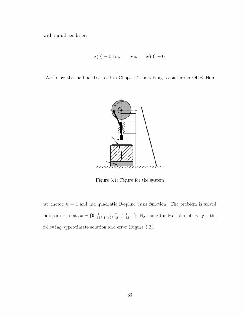
3.1. Mass spring system

A stamping machine applies hammering forces on metal sheets by a die attached

to the plunger[8]. The plunger moves vertically up-n-down by a flywheel spinning at

constant set speed (Figure 3.1). The constant rotational speed of the flywheel makes

the impact force on the sheet metal, and therefore the supporting base, intermittent

and cyclic. The heavy base on which the metal sheet is situated has a mass M = 2000

kg. The force acting on the base follows a function: F(t) = 2000 sin(10t), in which t

is time in seconds. The base is supported by an elastic pad with an equivalent spring

constant k = 2× 105 N/m. If the base is initially depressed down by an amount 0.1

m, what is the resonant vibration situation with the applied load ?

The above problem can be modeled by an ODE as follows

2000d2x(t)

dt+ 2× 105x(t) = 2000sin(10t),

32

with initial conditions

x(0) = 0.1m, and x′(0) = 0,

We follow the method discussed in Chapter 2 for solving second order ODE. Here,

Figure 3.1: Figure for the system

we choose k = 1 and use quadratic B-spline basis function. The problem is solved

in discrete points x = 0, 112, 1

4, 5

12, 7

12, 3

4, 11

12, 1. By using the Matlab code we get the

following approximate solution and error (Figure 3.2).

33

Figure 3.2: x approximate vs t and error for mass spring sysytem

3.2. Wave modeling

Consider one meter power line that is attached to poles at the end. Suddenly a

bird lands on the line, 1/3 away from one of the poles and flies away immediately.

The initial triangular shape modeled by the function (See Figure 3.3)

f(x) =

− 3

10x 0 ≤ x ≤ 1

3,

3(x−1)20

13≤ x ≤ 1.

34

How does the power line vibrate after the bird releasing the cord until it sets to rest?

The problem can be modeled as initial boundary value problem of a wave equation

[9].

∂2u

∂t2= c2∂

2u

∂x2, 0 < x < 1, t > 0,

where c = 1πms

, with the boundary conditions

u(0, t) = 0 and u(1, t) = 0 for all t > 0,

and the initial conditions

u(x, 0) = f(x).

The exact solution to the above PDE is

u(x, t) =9

10π2

∞∑n=1

sin nπ3

n2sinnπ cosnt.

We use quadratic B-spline basis function. Choose k = 1, so h = 16

and the partitions

on x axis will be 0 ≤ 16≤ 1

3≤ 1

2≤ 2

3≤ 5

6≤ 1. Furthermore, on t axis h = 10

6and the

partitions are 0 ≤ 106≤ 20

6≤ 5 ≤ 40

6≤ 50

6≤ 10 . After setting up the residuals at the

following discrete points and minimizing the sum of square errors at these points, we

will get the following errors (Table 3.1).

35

Figure 3.3: Initial position of the bird on the wire

x(m) t(sec) u exact U approximate error

0 2 0 0 00.2 2 0.329 0.3285 -5E-40.33329 2 0.478 0.4778 -1E-30.5 2 0.33729 0.33739 1E-40.8 2 9.21E-2 9.32E-2 1.1E-31 2 0 0 00 4 0 0 00.2 4 0.32869 0.32872 22E-50.33329 4 0.54759 0.54759 00.5 4 0.5602 0.5603 9.99E-50.8 4 0.31419 0.31409 -9.9E-51 4 0 0 00 8 0 0 00.2 8 0.3284 0.32827 -1.3E-40.33329 8 0.2536 0.25363 -6.99E-50.5 8 0.1147 0.114678 -2.199E-50.8 8 0.1295 0.12967 -1.7E-41 8 0 0 0

Table 3.1: The solution and the error for wave modeling

36

3.3. Diffusion equation

A doctor administers an intravenous injection of an allergy fighting medicine to a

patient suffering from an allergic reaction. The injection takes a total time T=5sec.

The blood in the vein flows with mean velocity u, such that blood over a region of

length L = uT contains the injected chemical. The concentration of the chemical in

the blood is C0. What is the distribution of the chemical in the vein when it reaches

the heart 80 s later?

The problem can be solved as a diffusion equation [11].

∂C

∂t= D

∂2C

∂x2

with initial distribution:

C(x, t0) =

C0 −L

2< x < L

2,

0 otherwise.

The analytical solution is

C(x, t) =c0

2

(erf(

x+ L2√

4Dt)− erf(

x− L2√

4Dt)

),

where erf is the error function and is defined as

erf(x) =2√π

∫ x

0

e−t2

dt.

37

The following data was found by talking to a physician

T = 3sec, u = 2 cm/s, C0 = 100 microgram/cc, D = 3.24× 10−3cm2/s.

Therefore, L = uT = 6cm. Now we will have:

C(x, t) = 50(erf(x+ 3√

12.96× 10−3t)− erf(

x− 3√12.96× 10−3t

))

we use quadratic B-spline basis and choose k=1. Now, on the x axis we have h = 1

and the partitions are −3 ≤ −2 ≤ −1 ≤ 0 ≤ 1 ≤ 2 ≤ 3. Furtheremore, on the t

axis h = 340

and we chose the partitions accordingly. We follow the discrete method

at x = −3,−2,−1, 0, 1, 2, 3 and t = 0, 10, 20, 30, 40, 50, 60, 70, 80. The result for

t = 80sec is presented below (Figure 3.4).

Figure 3.4: Approximate and exact concentration distribution of medicine and errorat 80 sec

38

CHAPTER 4 - COLLOCATION METHODS BY RADIAL

BASIS FUNCTIONS

4.1. Radial Basis Functions

Let φ : [0,+∞) → R be a univariate continuous function with φ(r) = φ(‖x‖),

where r = ‖x‖ =√x2

1 + x22 + ...+ x2

s for x = (x1, x2, ..., xs) in Rs. Below are a few

popular Radial Basis Functions (RBF).

1. Gaussian radial basis:

φ(r) = e−c2r2 ,

where c is the constant shape parameter given by

c2 =1

2σ2,

where σ2 is the variance of the normal distribution (Figure 4.1).

2. Multiquadric RBF:

φ(r) =√r2 + c2 for some c > 0.

39

Figure 4.1: Gaussian radial basis: left is centered at (10,10) with c=5, middle iscentered at (20,20) with c=3, right is centered at (30,30) with c=1

3. Inverse Multiquadric Function (IMQ)

φ(r) =1√

r2 + c2for some c > 0.

4. Generalized Inverse Multiquadric Functions:

φ(r) = (r2 + c2)−α, where c > 0 and α > 0.

The Gaussian and Inverse Multiuadric functions have the property

φ(r)→ 0 as ‖r‖ → ∞,

but this is not strictly necessary in solving differential equations below.

40

4.2. Kansa collocation methods

When we are given scattered data xi, fi, i = 1, ..., N,xi ∈ Rs, fi ∈ R, our goal

is to find an interpolant of the form [13]

P (x) =N∑j=1

cjφ(‖x− xj‖),x ∈ RS,

for some RBF φ, such that

P (xi) = fi, i = 1, ..., N.

Setting up the above equation will lead to

φ(‖x1 − x1‖) φ(‖x1 − x2‖) ... φ(‖x1 − xN‖)

φ(‖x2 − x1‖) φ(‖x2 − x2‖) ... φ(‖x2 − xN‖)

.

.

.

φ(‖xN − x1‖) φ(‖xN − x2‖) ... φ(‖xN − xN‖)

c1

c2.

.

.

.

cN

=

f(x1)

f(x2)

.

.

.

f(xN)

.

This linear system can be written as Ac = f , where the entries of A are

Aij = φ(‖x− xj‖).

41

It is known that A is non-singular for some radial functions like Multiquadratics,

Gaussians and Inverse Multiquadratic basis functions.

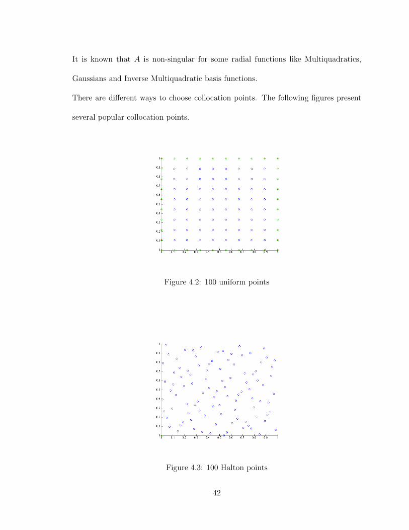
There are different ways to choose collocation points. The following figures present

several popular collocation points.

Figure 4.2: 100 uniform points

Figure 4.3: 100 Halton points

42

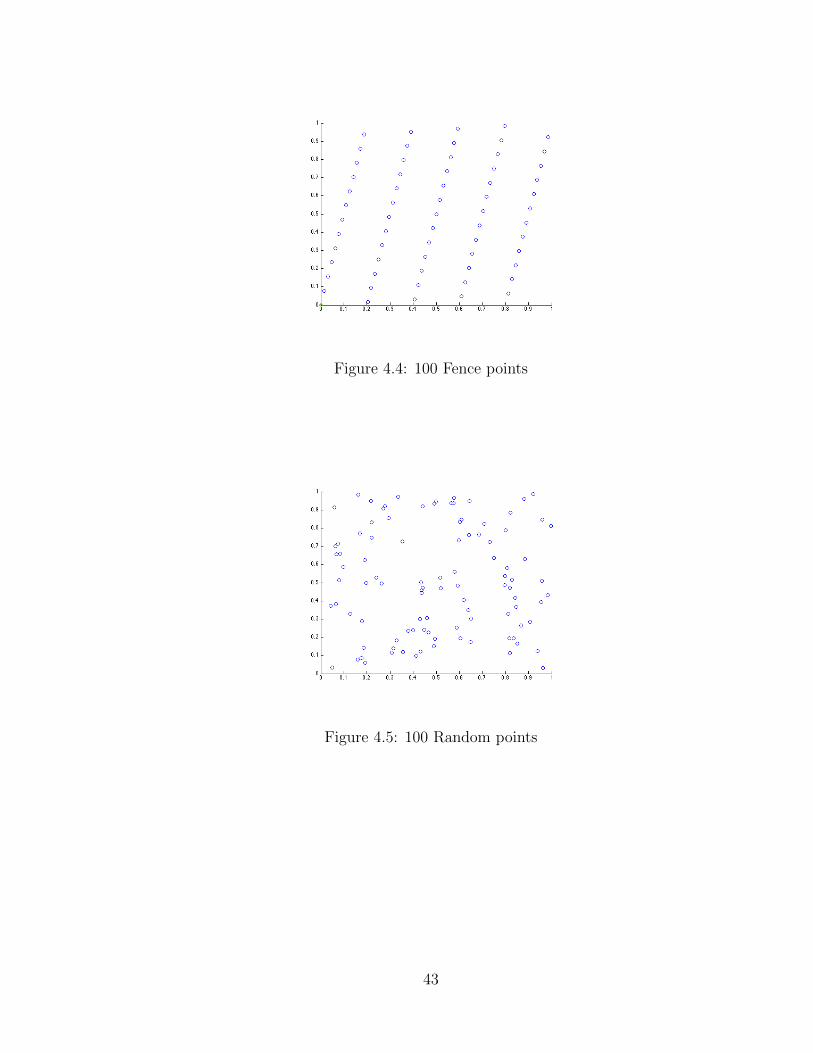
Figure 4.4: 100 Fence points

Figure 4.5: 100 Random points

43

Now consider solving a partial differential equation in the form of

Lu(x) = f(x), x ∈ Ω,

with Dirichlet boundary conditions

u(x) = g(x), x ∈ ∂Ω.

In Kansa’s collocation method, we choose the approximate solution in the form [10]

u(xi) =N∑j=1

cjφ(‖xi − xcj‖),

where xcj, j = 1, .., N, are the the centers and xi ∈ Ω , i = 1, .., k, or xi ∈ ∂Ω,

i = k + 1, ..,M, are the collocation points. Most of the times the centers and the

collocation points are the same set of points, or xi = xci . In this work we set the

collocation points and the centers equal, so M = N .

Now, we want to match the approximate and exact solution for the differential equa-

tions and boundary conditions at the collocation points. So matrix A becomes

A =

AL

A

,

44

where

Ac = f =

f(x1)

f(x2)

.

.

f(xk)

g(xk+1)

.

.

g(xN)

,

(AL)ij = Lφ(‖xi − xj‖), for xi ∈ Ω,

(A)ij = φ(‖xi − xj‖), for xi ∈ ∂Ω,

where xj, j = 1, .., N , are the centers. In this method RBFs that we can use are the

popular RBFs listed in section 4.1, but Kansa specifically used Multiquadratic form.

The above method is called Kansa Mesh-free method. The method collocates the

RBFs at each node without the need for mesh. The popular numerical solution of

PDEs by finite element methods needs creating mesh on the domain. This can be

difficult for irregular domain or higher dimensional domains. That is why the above

methods attract attention.

45

4.3. Solving PDEs by RBFs

Example 1: Solving Poisson’s equation with Dirichlet boundary condition:

Consider the following Poisson’s equation [12]

∂2u

∂x2+∂2u

∂y2= 6xy(1− y)− 2x3

for 0 ≤ x ≤ 1 and 0 ≤ y ≤ 1, where the Dirichlet boundary conditions are

u(0, y) = 0, u(1, y) = y(1− y),

u(x, 0) = u(x, 1) = 0.

This problem can be solved analytically, and the exact solution is

u(x, y) = y(1− y)x3.

We follow Kansa collocation method with Inverse Multiquadric and Gaussian RBF.

100 uniform and Halton collocation points have been used with in the domain and on

the boundary. For Gaussian and IMQ RFB, c = 3 was used. The results have been

compared (See Figures 4.6-4.7). As it can be seen uniform collocation form gives us

a better error in comparison with the Halton collocation points. Also, Gaussian RBF

was a better choice in comparison with IMQ.

46

Figure 4.6: Error for example of Poisson’s equation with 100 uniform collocationpoints by Gaussian RBF

Figure 4.7: Error for example of Poisson’s equation with 100 Halton collocation pointsby Gaussian RBF

47

Example 2: Poisson’s equation with Neumann boundary conditions:

Consider the following Poisson’s equation

∂2u

∂x2+∂2u

∂y2= −2(2y3 − 3y2 + 1) + 6(1− x2)(2y − 1),

for 0 ≤ x ≤ 1 and 0 ≤ y ≤ 1 with the boundary conditions

u(0, y) = 2y3 − 3y2 + 1,

u(1, y) = 0,

∂u(x, 0)

∂y=∂u(x, 1)

∂y= 0.

The analytical solution of this equation is

u(x, y) = (1− x2)(2y3 − 3y2 + 1).

We use Kansa collocation method with 100 Halton collocation points. Here IMQ

gives us the best error. We choose c = 3 and c = 10 in this example. As it shows,

c = 3 gives slightly better errors (Figures 4.8 and 4.9).

48

Figure 4.8: Error of an example of Poisson’s equation with Neumann boundary con-dition with IMQ RBF (c = 3) (using 100 Halton collocation points)

Figure 4.9: Error of an example of Poisson’s equation with Neumann boundary con-dition with IMQ RBF (c = 10) (using 100 Halton collocation points)

49

Example 3: Elliptic equation with variable coefficients:

Consider the following elliptic equation with variable coefficients and homogeneous

Dirichlet boundary conditions

−∇(α(x, y)∇u(x, y)) = F (x, y)

on the region Ω = [0, 1]× [0, 1], where

α(x, y) = 1 + x+ 2y2,

F (x, y) = x(1− x)(2 + 2x− 4y + 12y2) + y(1− y)(1 + 4x+ 4y2),

and boundary condition of

u(x, y) = 0, on ∂Ω.

The analytical solution is [50]

u(x, y) = xy(1− x)(1− y).

The above example was solved by Kansa collocation method. We choose IMQ RBF

and c = 3. 100 uniform collocation points were used (Figure 4.10).

50

Figure 4.10: Error of an example of Elliptic equation with variable coefficient withIMQ RBF (c = 3) (using 100 uniform collocation points)

Example 4: Solving a PDE with mixed boundary condition:

Consider

∇2u+ u = (2 + 3x)ex−y, (x, y) ∈ [0, 1]× [0, 1]

with the following mixed boundary conditions

u(0, y) = 0, u(x, 0) = xex,

∂u

∂x

∣∣∣∣x=1

= 2e1−y,∂u

∂y

∣∣∣∣y=1

= −xex−1.

The exact solution of this problem is [14]

u(x, y) = xex−y.

51

The problem was solved by using 100 Uniform collocation points by IMQ RBF (c = 3).

The result is followed (Figure 4.11).

Figure 4.11: Error of an example of PDE with mixed boundary conditions by IMQRBF (c = 3) (using 100 uniform collocation points)

4.4. Conclusion

Least square Method for Boundary Value Problems using B-splines discussed in

chapter 2, is an improved form of using B-spline basis functions [3]. Numerical Anal-

ysis contains little literature on higher order BVPs. In the papers by Loghmani all

the examples are higher order ODEs, but he suggested that the method works for

any linear and non-linear PDEs and system of elliptic PDEs. We used the method

for Poisson’s equation and the error was acceptable. As it can be seen in the ex-

amples, the accuracy of the method is efficient even with large partitioning of the

52

domain (k = 0 and k = 1). The Matlab program can take longer time to run for

solving PDEs. As we discussed earlier, meshfree methods introduced by Kansa at-

tract attention. In most popular finite element method, creating mesh was one of the

disadvantages. Creating mesh can be time consuming and costly especially for higher

dimensional and irregular shaped domains. Kansa Method is rather simple to use. He

suggests changing the shape parameter c to improve accuracy. The problem for this

method is that for a constant shape parameter c, the matrix A may become singular

for certain sets of centers xi. However, there is an approach that gives us strategies

to select a set of centers from possible points that ensure the non-singularity of the

collocation matrix [Ling et al. (2006)]. Kansa’s method has been extended by several

researchers to solve non-linear PDEs, systems of elliptic PDEs and time-dependent

parabolic and hyperbolic PDEs. Different methods have been suggested to improve

stability and it is an active research area.

53

REFERENCES

[1] Eason, Ernest D. A review of least square methods for solving partial differentialequations. International Journal for Numerical Methods In Engineering, Vol. 10,1021-1046 (1976)

[2] www.cs.mtu.edu/ shene/COURSES/cs3621/NOTES/spline/B-spline/bspline-ex-1.html

[3] Loghmani, M. AHMADINIA, Numerical solution of third-order boundary valueproblems. Iranian Journal of Science & Technology, Transaction A, Vol. 30, No.A3 (2006) 291−295

[4] Loghmani G.B, Application of least square method to arbitrary-order problemswith separated boundary conditions. Journal of Computational and AppliedMathematics 222 (2008) 500−510

[5] Yahya Qaid, Hasan.The numerical solution of third-order boundary value prob-lems by the modified decomposition method. Advances in Intelligent Transporta-tion Systems (AITS), Vol. 1, No. 3, 2012.

[6] Viswanadham, Kasi and Showri Raju. B-spline Collocation Method For SixthOrder Boundary Value Problems. Global Journal of researches in engineeringNumerical, Volume 12 Issue 1 Version 1.0 March 2012 Type: Double Blind PeerReviewed International Research Journal Publisher: Global Journals Inc. (USA)ISSN: 0975-5861

[7] G.B. Loghmani a,*, M. Ahmadinia. Numerical solution of sixth order boundaryvalue problems. Applied Mathematics and Computation 186 (2007) 992999

[8] Tai-Ran Hsu. Application of Second Order Differential Equations in MechanicalEngineering Analysis.http://www.engr.sjsu.edu/trhsu/Chapter%204%20Second%20order%20DEs.pdf

[9] Diffusion of point source and biological dispersal.www.resnet.wm.edu/ jxshix/math490/lecture-chap3.pdf

[10] Fasshauer, Gregory (2007). Meshfree Approximation Methods With Matlab.World science publishing company.

54

[11] Advective Diffusion Equation. https://ceprofs.civil.tamu.edu/ssocolofsky/cven489/downloads/book/ch2.pdf

[12] An example solution of Poisson’s equation in 2-dhttp : //farside.ph.utexas.edu/teaching/329/lectures/node71.html

[13] Meshfree methods. www.math.iit.edu/ fass/590/notes/Notes590Ch1Part3Print.pdf

[14] Liu and Y.T. Gu.(2005). An introduction to meshfree methods and their pro-gramming. Netherland. Springer.

55

CURRICULUM VITAE

Katayoun (Kathy) Kazemi

1901 Soaring ct, Las Vegas, NV 89134

Tel:(702) 218-4078 E-mail:kazemik3@unlv.nevada.edu

Education

• M.S. in Engineering Management, George Washington University, Washington

DC, 2014

• B.S. in Mechanical Engineering, Tehran Polytechnic University, Tehran, 2000.

Thesis: Comparing efficiency of cyclones in series versus parallel connection.

Employment

• Graduate Assistant and Mathematics Instructor

University of Nevada, Las Vegas, NV (1/2012-present)

• Mathematics Instructor Nevada State College, Las Vegas, NV (8/2004-1/2012)

• Mathematics Instructor University of phoenix, Las Vegas, NV (2004-2011)

• Mechanical Engineer Power Plant Projects Management Co. (MAPNA), Tehran,

Iran (4/2000-1/2002)

57