SOLUTIONS TO THREE-DIMENSIONAL THIN-LAYER … · solutions to three-dimensional thin-layer...

SOLUTIONS TO THREE-DIMENSIONAL THIN-LAYER NAVIER-STOKES

EQUATIONS IN ROTATING COORDINATES FOR FLOW

THROUGH TURBOMACHINERY

By

Amrit Raj Ghosh

A Thesis

Submitted to the Faculty of

Mississippi State University

in Partial Fulfillment of the Requirements

for the Degree of Master of Science

in Aerospace Engineering

in the Department of Aerospace Engineering

Mississippi State, Mississippi

December 1996

https://ntrs.nasa.gov/search.jsp?R=19980000490 2018-05-31T12:37:47+00:00Z

SOLUTIONS TO THREE-DIMENSIONAL THIN-LAYER NAVIER-STOKES

EQUATIONS IN ROTATING COORDINATES FOR FLOW

THROUGH TURBOMACHINERY

By

Amrit Raj Ghosh

Approved:

David_'_S_L._Jhitfiel-d/'

Professor of Aerospace Engineering(Director of Thesis)

Jo__ C. McWhorterGraduate Coordinator of theDepartment of AerospaceEngineering

,/9 ./ / ,.

_. Mark Janus

Assistant Professor of Aerospace

Engineering(Committee Member)

Jen-Ping Chen

Research Engineer, ERC

(Committee Member)

Richard D. Koshel t---

Dean of the Graduate School

A. Wdyne Bennett /

Dean of the College of Engineering

Name: Amrit Raj Ghosh

Date of Degree: December 13, 1996

Institution: Mississippi State University

Major Field: Aerospace Engineering

Major Professor: David L. Whitfield

Title of Study: SOLUTIONS TO THREE-DIMENSIONAL THIN-LAYERNAVIER-STOKES EQUATIONS IN ROTATING COORDI-NATES FOR FLOW THROUGH TURBOMACHINERY

Pages in Study: 73

Candidate for Degree of Master of Science

The viscous, Navier-Stokes solver for turbomachinery applications,

MSUTC has beenmodified to include the rotating frame formulation. The three-

dimensional thin-layer Navier-Stokes equations have been cast in a rotating

Cartesian frame enabling the freezing of grid motion. This also allows the flow-

field associated with an isolated rotor to be viewed as a steady-state problem.

Consequently, local time stepping can be used to accelerate convergence. The

formulation is validated by running NASA's Rotor 67 as the test case. Results

are compared between the rotating frame codeand the absolute frame code.The

useof the rotating frame approach greatly enhances the performance of the code

with respect to savings in computing time, without degradation of the solution.

DEDICATION

This thesis is dedicated to my parents, Nirmalendu and Krishna Ghosh,

and to the everlasting memory of my grandmother, Shanti Lata Bose.

ii

ACKNOWLEDGEMENTS

I would like to take this opportunity to express my sincere appreciation

and deepsenseof gratitude to Dr. David Whitfield for introducing me to the field

of CFD, his teaching, and his patience, understanding, and guidance through-

out the course of this work. Thanks to Dr. Mark Janus for being on my commit-

tee.

A special thank you to Dr. Jen Ping Chen for the guidance he provided

throughout this work, for painstakingly answering all my questions and queries

and for being on my committee. I am also grateful to Dr. Lafe Taylor and Dr. Abi

Arabshahi for getting me over the initial hang-up of understanding and running

a 3-D CFD code.I also thank Dr. Murali Beddhu for reading my thesis and mak-

ing valuable suggestions and clearing a lot of my doubts about the confusion of

reference frames. I am grateful to Dr. Z.U.A. Warsi for introducing me to the field

of tensors and removing my fear of superscripts and subscripts.

I would like to extend my warmest thanks to all my friends for making

my stay here, one of the most memorable phases in my life. Sreenivas, 'the an-

swer guy', for helping everytime I went and cried to him about anything. Shyam,

Rajeev,and Rambabu for their support, encouragement and advise. Laxman, for

being a good friend and helping me out in my time of crisis. Pradeep 'Bhaisaab'

and Bhabhiji for providing me with foodand shelter and for always boosting my

spirits when I was going through trying times. Ramesh, for his jibes about my

graduation. Gayatri, Vikram and Minnie for all those nice parties. And to Rao,

oo°

111

Goyalia, Krishnaraj, Sanjay, Gill, Aditya, Edward, ND, Rahul, Lokesh, Rizwan,

Dilnaz, Sudeep and Nivu for all the good times we shared together.

This research was supported by NASA Lewis Research Center under

Grant NAG-3-1712, Dr. Eric McFarland, Contract Monitor. Computing time was

provided by NSF Engineering Research Center at MSU.

iv

TABLE OF CONTENTS

Page

DEDICATION ...................................................... ii

ACKNOWLEDGEMENTS ........................................... iv

LIST OF TABLES .................................................. vii

LIST OF FIGURES ................................................. viii

CHAPTER

I. INTRODUCTION .......................................... 1

II.

III.

GOVERNING EQUATIONS ................................. 4

2.1 Continuity Equation .................................. 8

2.2 Momentum Equation .................................. 8

2.3 Energy Equation ...................................... 9

2.4 Conservation Law Vector form of the Equations .......... 9

2.5 Non-Dimensionalization of the Equations ............... 13

2.6 Curvilinear Coordinate Transformation ................. 14

2.6.1 Thin-Layer Approximation ...................... 19

NUMERICAL SOLUTION METHOD ....................... 22

3.1 Finite Volume Discretization ........................... 22

3.2 Implicit Formulation .................................. 23

3.3 Newton's Formulation ................................. 24

3.3.1 Flux Vector Splitting ........................... 26

3.3.2 Viscous Flux Jacobian .......................... 27

3.4 Flux Formulation ..................................... 28

3.4.1 Convective Flux Computation ................... 28

V

CHAPTER Page

3.4.2 Diffusive Flux Computation ..................... 29

3.4.3 Turbulence Modeling ........................... 30

3.5 The N-Pass Scheme ................................... 31

3.6 Boundary Conditions .................................. 32

3.6.1 Subsonic Outflow .............................. 32

IVo RESULTS ................................................ 37

4.1 Rotor 67 .............................................. 37

V. SUMMARY AND CONCLUSIONS .......................... 55

REFERENCES .................................................... 57

APPENDIX

Ao DERIVATION OF THE VELOCITY OF THE MOVING

COORDINATES ....................................... 59

So CURVILINEAR COORDINATE TRANSFORMATION OF THE

NAVIER-STOKES EQUATIONS ........................ 62

C. CYLINDRICAL COORDINATE FORMULATION ............ 68

vi

LIST OF TABLES

TABLE

4.1

Page

Performance Enhancement ................................. 40

vii

FIGURE

2.1

3.1

3.2

4.1

4.2

4.3

4.4

4.5

4.6

4.7

4.8

4.9

4.10

4.11

4.12

4.13

4.14

LIST OF FIGURES

Page

Rotating Cartesian Coordinate Frame ....................... 6

Unit Volume Computational Cell ........................... 22

Codirectional Outflow ..................................... 33

Mass Flow History (back pr. = 0.75) ......................... 43

Mass Flow History (log-linear, back pr. = 0.75) ............... 43





Mass Flow Ratio History (back pr. = 0.75) ................... 46

Mass Flow Ratio History (log-linear, back pr. = 0.75) .......... 46





Relative Mach No. Contours at 10% Span for Near Peak

Efficiency .............................................. 49


Efficiency .............................................. 50

ooo

Vlll

FIGURE

4.15

4.16

4.17

4.18

A.1

Page


Efficiency .............................................. 51

Relative Mach No. Contours at 10% Span for Near Stall ...... 52



Plane of Rotation .......................................... 60

ix

CHAPTER I

INTRODUCTION

The flow field associated with turbomachinery applications is very com-

plex. This flow field is highly unsteady, involving a wide range of time and

length scales [1]. The goal of a CFD code for simulating such flows is to be able

to model all aspects of the flow phenomena reasonably well. The computing time

that is required should also be practically feasible for the CFD code to be useful

as a design tool for turbomachinery applications.

The MSUTC code, which is a turbomachinery flow analysis research tool,

is an attempt to achieve this goal. This code has been under development at the

NSF ERC for Computational Field Simulation at Mississippi State University.

It is a viscous flow solver which is capable of simulating even or uneven-blade-

count, single-rotating, counter-rotating or rotor-stator, axisymmetric or non-

symmetric, multistage, at angle-of attack geometries. Chen [2] noted that

though converged unsteady solutions can be obtained using the above code, they

are very expensive, because the use of Newton sub-iterations requires tremen-

dous computing time. Thus, the performance of the code can be enhanced if one

can avoid the Newton sub-iterations.

Navier-Stokes equations which are the governing equations of fluid me-

chanics can be expressed in the vector invariant form so that they are indepen-

dent of the coordinate system. For flows in rotating machinery, it is convenient

to cast the equations in the rotating coordinate system. Adamcyzk et al. [3] cast

2

the equations in a rotating cylindrical coordinate system to simulate viscous

flow through turbines. Although unsteady computations are very important in

turbomachinery simulation, many of the problems canbeviewed assteady-state

problems in the rotating frame, e.g. an isolated rotor. Consequently, local time

stepping and multigrid methods can be utilized to accelerate convergence.

Due to this motivation, at the start of this study an effort was made to de-

velop a cylindrical coordinate system Navier-Stokes code for simulating the

steady flow through a single blade row machine. During the course of the inves-

tigation it was realized that only a few modifications were necessary to incorpo-

rate the rotating frame formulation into the existing unsteady code if one re-

tained the Cartesian coordinate system but solved the problem in a rotating

frame similar to the approach in [4] and [5]. This is the approach that was

adopted for the work presented in this study. The existing viscous solver is modi-

fied to include the rotating frame formulation using the absolute velocity vector.

This thesis is divided into five chapters. Chapter II develops the govern-

ing equations cast in the rotating Cartesian coordinate frame. The velocity used

in the equations, however is the absolute velocity represented in the rotating

frame. The equations are then non-dimensionalized and transformed from Car-

tesian coordinates to steady curvilinear coordinates to enable the use of a body

conforming grid. The thin layer approximation is also explained in this chapter.

Chapter III describes the aspectsof the flow solver with all the changes that are

made due to the change in the formulation. The implicit formulation, Newton's

method, flux formulation, flux Jacobians, the N-Pass solution scheme and the

boundary conditions are all explained and discussed in this chapter. Chapter IV

3

presents the results obtained from the modified code. The test case used is

NASA's Rotor 67. The results obtained from the rotating frame approach are

compared with those obtained form the absolute frame approach. Chapter V is

devoted to summary and conclusions.

CHAPTER II

GOVERNING EQUATIONS

The development of the Navier-Stokes equations in the rotating coordi-

nates are presented in this chapter. The primary objective in this study is to

make use of the quantities in the fixed frame formulation so that a minimum

amount of changesneedto bemade to the existing code.Toachieve this goal, the

formulation presented in this chapter develops the Navier-Stokes equations in

rotating coordinates using the absolute velocity, i.e. velocity with respect to the

fixed inertial frame.

The differential forms of the equations of conservation of mass, momen-

tum and energy can be collectively stated in a general form. The differential

form of the general conservation principle can be stated as [6]:

0.4 + div f = C (2.1)ot

where f = Au + B and A, B, C, are tensor quantities such that A and C

have the same tensorial order, and if B # 0 then it is an order higher than

A and C. Equation (2.1) is written with respect to an inertial frame so that the

vector u is the absolute velocity. Consider a transformation from the inertial

frame to a moving non-inertial frame which is of the form [6]:

X i = xi(Xl,X2,X3, t), i = 1,2,3 and v = t

4

5

where (Xl, x 2, X 3) are the rectangular Cartesian coordinates defining the some-

how, inertial frame. (x 1, x 2, x 3) are the general coordinates defining the mov-

ing frame and a are the covariant base vectors of the moving frame. If the rela---i

tive velocity of a fluid particle, which is the velocity with respect to the

nonsteady coordinates, is denoted by v and the velocity of the moving coordi-

nates is denoted by w; the absolute velocity of a fluid particle can be expressed

by the following equation [6]:

u = v - w (2.2)

where

Oxi (2.3)w = -- a_ Ot -i

The contravariant components of w are the partial time derivatives of each of

the coordinates in the moving frame and it can be proven to be negative of the

velocity of the moving frame with respect to the inertial frame. Thus, the vector

w can be thought of as the velocity of the absolute frame, which an observer in

the rotating frame would notice. Details of the derivation are presented in Ap-

pendix A.

Due to the above transformation, the following relation exists between the par-

tial time derivatives in the two frames of reference [6]:

0( ) 0( )- + w grad( ) (2.4)

Ot Or _

Thus, the unified conservation law, equation (2.1), transforms to [6]"

6

0.4 + (gradA) • w + div f = C (2.5)

The rotating Cartesian coordinate frame utilized in this study is illustrated be-

lOW.

t_

Y

/\

/Z

> X

Figure 2.1 Rotating Cartesian Coordinate Frame

It is evident from Figure 2.1 that the rotating frame is rectangular Carte-

sian in nature, due to which there is no distinction between covariant and con-

travariant components. Also the base vectors do not vary in space, so that:

Oa-j

- 0dx i

(2.6)

The temporal derivatives of the base vectors are given by [6]:

Oa Ow-i + - - 0 (2.7)

Ov c)xi

Choosing a rotating frame illustrated in Figure 2.1 results in: w = - _2 x r

where Y2 = - YJa . Therefore, w = - Qx3a + Qx2a . Consequently,- -1 - -2 -3

c_wdiv w = _ • a i - OwJ a • a i - Owi - 0 (2.8)

_ c)Xi _ c_Xi -j _ Ox i

Using the following tensor identity •

div (Aw) = (grad A) • w + (div w)A = (grad A) w (2.9)

and equation (2.8), one can rewrite equation (2.5) as:

0,4 + div (Aw) + div f = C (2.10)0r

As explained at the beginning of this chapter, the primary objective is to

cast the Navier-Stokes equation in the rotating frame using the absolute veloc-

ity vector. The continuity, momentum and energy equations that are derived be-

low in this chapter, have used the absolute velocity vector u. However, all the

vectors appearing in equation (2.10) are represented using the base vectors of

the rotating frame. This concept can appear confusing. This confusion is re-

moved by addressing two important aspects related to any velocity vector in the

above equations. The first being definition of the vector, and the second is repre-

sentation of the vector.

The keywords to defining a velocity vector are: with respect to. This clari-

fies which reference frame one is referring to when defining the velocity vector.

Thus, the absolute velocity u, is defined as the velocity of a fluid particle in the

concerned flowfield, with respect to the fixed inertial frame. Therefore, a station-

ary observer who selects a right handed rectangular coordinate system like the

one in Figure 2.1, but one which is not moving, observes the velocity of a fluid

particle in the flow field as u. On the other hand, an observer moving with the

8

axesdescribed in Figure 2.1, observesthe velocity ofthe fluid particle in the flow

field as v. Thus, the relative velocity v, is defined as the velocity of a fluid par-

ticle with respect to the rotating non-inertial reference frame.

Once the definition of the vector is taken care of, the issue of representing

the vector arises. These two issues are independent of each other and once a vec-

tor is defined with respect to a frame, there is no need to express the components

of the same vector using a coordinate system in the same frame. Thus, the abso-

lute velocity vector can be expressed in component form with respect to the basis

of the rotating Cartesian coordinate system shown in Figure 2.1. Since the exer-

cise in this chapter is to cast the Navier-Stokes equations in the rotating frame,

all the mathematical operations arising in the equations below, viz., time deriv-

atives, curl, grad, div, are carried out in the rotating frame and involve its base

vectors. To be consistent and to simplify mathematical operations, the rotating

frame has been chosen to represent all vectors and tensors.

_.1 Continuity Equation

The continuity equation is obtained from the generalized conservation

law, equation (2.10), by substitutingA = _, f = Qu, B = 0, C = 0. Thus,

the continuity equation in the rotating frame can be written as:

0Q0-_ + div (Qw)_ + div (Qu)_ = 0 (2.11)

2.2 Momentum Equation

The momentum equation in the non-inertial frame is obtained by substi-

tutingA = Qu, B = - T = p I - a, C = O in equation (2.10).

9

The resulting equation is:

O(Qu )

or + div (_uw) + div (Quu) = div (T) (2.12)

where T is the stress tensor, p is the thermodynamic static pressure, I is the

identity tensor and a is the deviatoric part of the stress tensor containing the

viscous shear stress. It can be represented by:

= 2(div u)I + tt[(grad u) + (grad u) T] (2.13)

wherett and 2 are the first and second coefficients of viscosity, respectively. Writ-

ing u = u_a and utilizing the result in equation (2.7), the momentum equation

can be rewritten as:

v,e ,z:'ui_ _ . Owo_a + div (Ouw) + div (Ouu) = div (T) + OU_ox i (2.14)

_g ....

2.3 Energy Equation

The generalized conservation law, equation (2.10), yields the energy

equation by substituting A = et, B = - T" u + q, C = 0, where

Pm

et _-1_ __ + lp Iu I 2 is the total energy and q is the conductive heat flux vector.

The energy equation in the rotating frame, therefore, is:

lge t

0--r" + div (etw)_ + div (etu)_ = div (T-u)_ - div(q) (2.15)

2.4 Conservation Law Vector form of the Equations

Equations (2.11), (2.14) and (2.15) can be expanded and written in the

10

conservation law form by carrying out the mathematical operations of diver-

gence and dot products on the various vectors and tensors involved. While doing

the operations involving the base vectors one utilizes the results that the base

vectors do not vary in space and that since the coordinate axes are rectangular

Cartesian in nature; a i " aj = _ij" For simplicity, let

x 1 = x, x 2 =y, x 3 =z, v = t and u 1 = u, u 2 = v, u 3 = w. The five equa-

tions that result can then be combined into one single vector equation of the

forIn:

Oq Of Og Oh OF + Ogv + Oh _ + s (2.16)O---i +-g-_ +g-y + Oz - Ox 03, 07

where the dependent variable vector q, the flux vectors f, g, h, the viscous flux

vectors fv, h v, gV, and the source term vector s are defined as follows:

q

Ow

et

(2.17)

f

Qu

Ou 2 +p

Quv

_uw

u(e t + p)

g

Ov - _Qz

Ovu - Ou_z

QV 2 + p -- QvQz

Qvw - OwQz

v(e t + p) - et.Qz

h

Ow + QQy

Owu + QuQy

, Owv + Qv_yII _ w2 4- p 4- Ow_y

w(et + p) + et.Qy

(2.18)

0 ]Z'xx

Vxy

Txz

-I- VTxy q- W_'xz q-qx

gU

UTyx+

0

ryx

Tyy

ryz

Vryy + WVyz + qy

11

(2.19)

hV 0 ]"gzx

T'zy

Tzz

+ VZ'zy + WTzz + qz

S

0

0

- Ow_

OvQ

0

(2.20)

The viscous stress terms appearing in the equation (2.19) are defined below un-

2der the assumption that bulk viscosity is negligible, so that 2 = - _p.

Vxx = 2it(20u Ov Ow)-_ 03, Oz'

"gyy = _p(2 Ov Ou Ow03, Ox _ )'

Vzz = _/_(20w Ou Ovoz ox -_) '

OU OV

"gxy = "gyx = _('-_ q- -ff'_)

Ov OwT.yz = Tzy = _U("_ "1- "-_')

Ow Our_x = r:,z = _(--ff + -_)

(2.21)

The conductive heat flux terms which appear in the viscous flux vectors are de-

fined below. The conductive heat flux vector is defined as: q = - k(grad T)

where k is the thermal conductivity, and T is the temperature. The components

of the heat flux vectors along each of the coordinate directions, therefore, are:

12

q. = k OTOx

qy = k o7' (2.22)Oy

qz = kOTOz

All the components of the tensors and vectors that appeared in the equa-

tion (2.16) are in terms of the base vectors of the rotating frame. The existing

code uses a fixed frame formulation so that the components involved are in

terms of the base vectors of the fixed frame. For the purpose of validation of the

rotating frame formulation one needs to be able to compare the flow fields gener-

ated as the solutions from the two formulations. Thus, a relation between com-

ponents in the rotating frame and components in the fixed frame needs to be ob-

tained. Letting Ua, Va, and Wa be the components of the absolute velocity with

respect to a Cartesian coordinate system in the fixed frame, and, assuming for

convenience, that the initial configuration of the rotating frame matches with

the stationary frame (say at instant t = 0); the following relations are obtained:

U a = U

Va = v cos(tgt) - w sin(_2t) (2.23)

Wa = v sin(t2t) + w cos(t2t)

where, it is emphasized that u, v, and w are the components of the absolute

velocity with respect to a rotating Cartesian basis. It is apparent from the above

equation that at instant t = 0 and after every subsequent full rotation, the com-

ponents of the absolute velocity in the rotating frame are identical to the compo-

nents in the stationary frame.

Now, the Navier-Stokes equations have already been cast in the moving

frame, so that there is no need to move the grid anymore. The flow field that is

13

generated in terms of the components, by solving the Navier-Stokes equations

in the form presented in equation (2.16), for purposes of comparison, can be

changed according to equation (2.23) to match the flow field which results from

solving Navier-Stokes equations derived in the inertial frame. However, the dis-

tinct advantage of the former over the latter is that local time stepping can be

used for steady flows in the rotating frame. Another advantage is the freezing

of grid motion becausein the fixed frame formulation the grid motion is impera-

tive.

2.5 Non-Dimensionalization of the Equations

All the variables used in the formulation till now are dimensional vari-

ables. In order to obtain a form of the equation (2.16) with non-dimensional

quantities, a scaling of all the dimensional variables (denoted by ^ ) is carried

out using the following relations:

x=--z, y =-z , z=--z, u =-;--, v =-z-, w =-;--, t2 =-7--D D D ao ao ao ao

P_ a°t e h - = --

=-^ ^---_, Q = 7--, t =--;-, e =-^ ^---5' ---_, It ^Qoao Qo D _oao ao t_o

^ ^ ?Ix, T T ^2 ^^TiJ Twall qxi ^ ^ 3 ' '- - , = = -7- ao = yRT 0

V iJ ^ ^2' V wall , _ ,_o \

Q°a° ( D )'--r-- Ooao To

The scaling has been accomplished using the reference quantities (de-

noted by subscript 0) which are the total conditions and the reference length/)

which is the maximum diameter of the blade tip. The detailed development of

the scaling of the equations can be found in [2]. The scaling results in a form of

14

the vector equation which is exactly similar to equation (2.16) but with non-di-

mensional variables. The form of the dependent variable, flux, viscous flux and

the source term vectors is also exactly sameasshown in equations (2.17) - (2.20),

but with all variables non-dimensional. The only difference arising out of the

scaling of equations is the introduction of two new non-dimensional quantities,

viz., Reynolds and Prandtl numbers (Re, Pr), which appear in the non-dimen-

sional form of the viscous shear stress and the conductive heat flux terms. The

non-dimensional viscous shear stress and the conductive heat flux terms are:

1 2 au av Ow 1 ,au avVxx - l_e_tt(2 _-_ 03, _-)' Vxy = ryx = _-_w,.._ + -_)

1 2 av au aw 1 ,av aw_yY- _-_-_t'(2 Oy Ox _)' _yz = _zy = _-_t-_ +-y-y-)

_ 1 2 aw Ou av 1 .,aw auVzz Re p(2 az ax _)' rzx = rxz = _eett_--_ + -_)

(2.24)

qx

qy

qz

Re (_ - 1) Pr

1[Re (_,- 1)Pr

aT_x

aT

oy

aT

(2.25)

^ ^

where Re - 0°a°D and Pr _ Cp I_^

2.6 Curvilinear Coordinate Transformation

In order to carry out numerical computation of the governing equations

on a configuration comprising of a complex geometry, it is simpler to use a body-

conforming grid in which the solid surfaces in the geometry correspond to

15

constant coordinate surfaces. To this end, a curvilinear coordinate transforma-

tion needsto be introduced in the rectangular Cartesian spacebeing used in the

formulation thus far. The following general, nonorthogonal, steady, curvilinear

coordinate system is introduced in the (x, y, z) space:

= _(x,y, z)

r� = r/(x,y,z)

= ¢(x,y,z)

T=t

(2.26)

Only the final results due to the transformation are stated in this section. A de-

tailed presentation of all the steps involved and the how the relations for the

metric terms are obtained, is made in Appendix B. Using chain rule yields:

0 _ 0at Or

Ox

c9 -- ,y-_ -F O Cy__oy r/yT +

o +r/zT +¢zOz

(2.27)

The Jacobian J of the inverse transformation is:

_ IO(x,y,z)l

J = detlo- , ,

= x_(y_z_- z_y_) - y_(x_z_- z_x_) + z_(xrty_- y_x¢)

(2.28)

The metric terms in equation (2.27) are:

_x = _(yrtz¢-z_) r/x = _(z_y_-y_z¢) Cx = _(y_z_- z_y_)

_y = _(Zr/X_- Xr/Z_) r/y = _(X_-Z_- Z_X_) _y = X(z_r/- X_-Zr/)(2.29)

1 - x_y_) _z = --_(x_y_ - y_x_)l(x_y¢-yrtx¢) r/z = _(y_x¢3

16

Substituting relations obtained in equation (2.27) into equation (2.16) re-

sults in the form of the governing equations in stationary curvilinear coordi-

nates. Only the final equation is stated here. The resulting form is:

_ OH voQ OF OG OH OF v OGv + + S (2.30)

where

Q=J

ol)U

ee]

(2.31)

K=J

oK'

QuK' + kxp

QvK' + kyp

QwK' + kzp

etK' + pK

where K' = kxu + kyv + kzw + k t

k t = - kyQz + kz_Jy

K= kxu + kyv + kzw

(2.32)

i;_ = J

.

T,zQk

(2.33)

S=J

0

0

- Ow_2

OvQ

0

(2.34)

In the above equations (2.32) and (2.33), K = F, G, H; K' = U', V', W';

K = U, V, W; i_ = F v, G v, HV; for k = _, t], _ respectively. The appear-

ance of the term k t is to account for the divergence terms in equations (2.11),

17

(2.14), and (2.15) in which the vector w explicitly appears. This can be further

explained by considering the continuity equation, the treatment being same for

the other equations. The continuity equation can be rewritten as:

000-7 + div [_(u_ +w)_ ] = 0 (2.35)

which in curvilinear coordinates becomes

o(Jo)Ot + 0.._0.[Jo(u + w) • a k ] = 0 (2.36)

Ox k - _ _

It can be verified that:

and

k t = w" a k (2.37)

K' = (u + w) • a k (2.38)

In the formulation of the continuity equation in the absolute frame the term k t

appears in a strikingly similar manner and denotes the contravariant compo-

nent of the grid velocity vector. In the present formulation, however, there is no

grid motion involved and k t should not be associated with any grid velocity. It

is just the contravariant component of the vector, w = - Q x r. The expres-

sions for transformed shear stress and heat flux terms are as follows:

Tkx = kxvxx + kyvyx + kzzzx

Tky = kxvxy + kyvyy + kzvzy

Tkz = kxvxz + kyvyz + kzvzz

Qk = uTkx + VTky + wT_ + kxqx + kyqy + kzqz

(2.39)

where

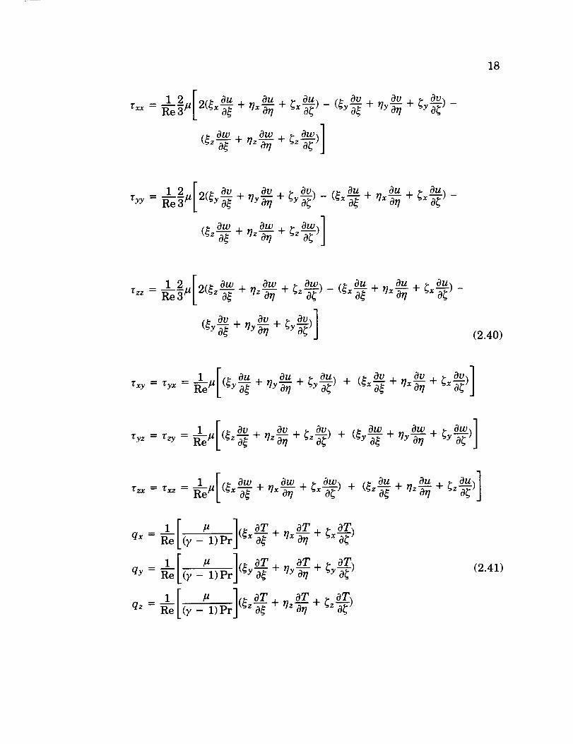
18

=12[ Ou Ou OU (_y_ q- _y_ + _y_) -

(_(+ _z_-_+ ;z_-;)1

"_yy

8u Ou Ou

1 2 Ow Ow -_) (_xVzz _-#[ += 2(_-ff ,7_-_+ _ _, - -_ + ,7_ + _x-_) -

Re3 [

ov o_)](_Y_o¢+ _Y-_ + _y(2.40)

°v1) + (_x + -_

= 1 Ou Ou Ou Ov Ov

1 .[(_ ow ow l;,,_) + (,_°u ou ]

_e[ # Prl]_e oT + ___aT + aT

1 [ # ],e OT aT + aT- -- " _-- _sY aqY - Re[(y - 1)Prl _ + r/y--_ _,y-_)

(2.41)

oQ oF

0-7where

19

2.6.1 Thin-Layer Approximation

Since the numerical simulation of the full Navier-Stokes equations are

very computationally intensive, the thin-layer approximation is used in this

study. This approach is useful because it can handle flows which have both invis-

cid and viscous regions and interactions between the two [2]. The thin-layer

approximation makes use of the fact that most grids for Navier-Stokes equa-

tions are packed in the direction normal to the walls, whereas along the stream-

wise direction they are usually very coarse and good enough for inviscid calcula-

tions only [2]. In this study, _ is the streamwise, 77 the spanwise, and _ the

pitchwise directions. Thus, all the viscous and heat flux derivatives in the

streamwise direction are dropped. In the other two directions, only the normal

second derivatives are considered while the mixed derivatives are neglected.

This is done because they are insignificant in corners and lead to expensive cal-

culations [2]. Applying the above approximation to equation (2.30) gives the fol-

lowing final form of the governing equations:

oG OH OGv OHv+ -_- + 0_ - 0rl + 0_ + S (2.42)

Q = j (2.43)

F=J

JQU'

mU' + _p

_vU' + _yp

owU' + _zP

etU' + pU

G=J

oV'

ouV' + r/xp

ovV' + r/yp

owV' + r/zP

etU' + pV

,H=J

oW'

ou W' + _xP

ovW' + _yp

owW' + _zP

etW' + pW

2.44)

GV=J

01T_x

Q_

HV =j

"0"

Q_

2O

(2.45)

S=J

0

0

- Owt'2

OvQ

0

(2.46)

The terms U', V', W', and U, V, W are defined in equation (2.32). The ex-

pressions for the transformed shear stress and the transformed heat flux terms

appearing in the viscous flux vectors are:

Tkx = kxrxx + kyvyx + kzvzx

Tky = kxvxy + kyvyy + kzrzy

Tkz = kxvxz + kyvyz + kzvzz

Qk = uT_ + VTky + wTkz + kxqx + kyqy + kzqz

(2.47)

In the equation (2.47) above, k = _], _ for flux vectors G v, H v respectively.

Applying the thin-layer approximation in the k direction the viscous stress and

the conductive heat flux terms will become:

_ 1 2 .[,,_ _,_, Ov Owlrxx - _ee-_/u[_x"_-_- ky'_- ]_z"_J

_ 1 2.[,,,_ vv oU_kz_g __yy- g_gF,[_.,_y_- kxg

_ 12 [, Ow Ou Ov]rzz Re-3P "_kz Ok kx-_ - ky

(2.48)

21

[k ou k_'xy _- "gyx = ,uLy Ok -.I- x Ok J

1. [k Ov k owlVyz = Vzy = -_eettL z-_ + y ok J (2.49)

rzx = _xz = tt kx--_ + kz

qx = (7- 1)Pr -_-)

qY ---- (_'- 1)Pr _) (2.5o)

qz = (7 - 1) Pr

The approach described in this chapter for the development of the govern-

ing equations was not initially employed for this study. The initial route taken

was via the cylindrical coordinates. However, it was later realized that the ap-

proach described above is much more elegant and less time consuming. It also

entails the minimum amount of changes to the existing code for it to work for

this particular formulation.

For completeness, the development of the governing equations using cy-

lindrical coordinates in a rotating frame is presented in Appendix C. The final

form of the equations derived in Appendix C are then transformed from cylindri-

cal to Cartesian coordinates to see if they match the governing equations derived

here in this chapter.

CHAPTER III

NUMERICAL SOLUTION METHOD

The finite volume approach is utilized to obtain the numerical solution

of the thin-layer Navier-Stokes equations which were derived in the previous

chapter and are presented in their final form in equation (2.42).

3,1 Finite Volume Discretization

The curvilinear coordinate transformation maps the entire physical do-

main to a computational domain which is discretized into collection of cells of

unit volume. Thus, A_ = A_/ = A_ = 1. The finite volume formulation is ob-

tained by integrating equation (2.42) over a unit volume computational cell,

which is shown in the figure below.

fiII •

I (i, j, k)IF

/J

//

l

/_____>

Figure 3.1 Unit Volume Computational Cell

22

23

In the cell-centered finite volume approach the dependent variable vector Q, is

assumed to be the flow quantities at the cell center, and is uniform throughout

the cell. The fluxes F, G, H, G v, H v are assumed to be uniform over each cor-

responding cell face. The integral form of equation (2.42) after spatial discreti-

zation, can then be written as:

-_r A_AyA_ + (F i 1- Fi_½)ArIA_+-_V

+ [(Vj+__ - Vj___) - (Vj+½ V vs__I)]A_A_

+ [(H k +_1 - Hk_ ½) - (H_k +_1- HVk_½)]A_Ari

Defining the central difference operator _ as _l ( ) = ( )l+½ - ( )/ _½ and not-

ing that the finite volume cell has sides of unit length, equation (3.1) can be re-

written as:

oQO-r- + hi(F) + 6j(G- G v) + 6h(H- Hv) = S (3.2)

In the above definition of 6, l + 1 represents the face adjacent to the cell center

in the positive direction of l and l - 1 represents the face adjacent to the cell

center in the negative direction of/, where l = i, j, k fort, r/, _ directions re-

spectively.

3.2 Implicit Formulation

An implicit scheme is utilized to numerically integrate equation (3.2) be-

cause these schemes can handle large CFL numbers. In problems involving vis-

cous computations, very fine grid spacing is chosen to resolve the viscous effects,

due to which the tolerable minimum time step cannot be too small for the code

24

to have any practical value [2]. A first-order time-accurate implicit scheme to

numerically solve equation (3.2) can be implemented by the following algebraic

equation:

/iQn = _ /iv (R n+l)

where

/iQn =

Rn+l =

(3.3)

Qn + l _ Qn

6 i (F) n+l + 6j (G) n+l + 6 k (H) n+l

6j (GV) n +1 _ 6k (Hv)n+l _ sn+l

(3.4)

As can be observed from the above equation, the convective and diffusive fluxes

and the source term are all treated implicitly.

3.3 Newton's Formulation

The Newton's iteration method is used in this work to solve equation

(3.4). A detailed explanation of the method is presented in [2] and [7]. For a sys-

tem of nonlinear equations the Newton's method can be stated as [7]:

F,(x k) (x k+ l _ x k) = _ F(x k) (3.5)

Dividing equation (3.3) by J, will result in

= - A--_ (R n + 1) (3.6),4q n

where

/iv = d__[v (3.7)J

The Newton's method can now be applied to the following vector equation:

L(qn+l) = 0 (3.8)

where

25

L(qn+l) = qn+l _ qn + ,_ (Rn+l) (3.9)

The resulting matrix equation is:

[ I - _-_ (__qS)*,k-1 + _-_ (M)*,k-1 "l Aq k-1

_ [qk-1 _ qn + Av (R *'k-l) ]

(3.10)

The operator • indicates that the difference operator M acts on the delta form

of the unknown vector Aq k- 1, where Aq k- 1 = qk _ qk-1 [2]. It can be ob-

served from equation (3.10), that the time derivative term is present in the resid-

ual which arises by applying the Newton's method to the nonlinear system of

equations. The sub-iterations help in obtaining a better approximation of the

solution at each time step. This method, is therefore, better for unsteady prob-

lems. The various operators and terms appearing in equation (3.10) are defined

as follows:

M*,k-1. = 5i (A)*,k-1. + Sj (B) *'k-l" + Sk (C)*,k-1. _

(_j (BV)*,k- 1 . _ 5k (CV)*,k- 1

OF OG C- oH B v OG v C v_ OH vwhere A =-b-q' S = 0--q-' - 0-_' = 0--q- ' Oq

R*,k-1 = 6i (F)*,k-1 + Oj (G)*,k-1 + (_k (H)*'k-1

(_j (GV)*,k-1 _ (_k (HV)*'k-1 _ s*,k-1

(3.11)

The superscript * is used in the above equation to specify the time level

for computing the metric terms. Janus [13] found that in order to maintain the

mass flow without discontinuities when crossing the interface between a rotor

and a stator, the metric terms at old time level n and q0 should be used for the

first iteration. For the subsequent iterations, the metric terms at the present

26

level n + 1 and qk - 1 are used. A, B, and C are the flux Jacobians, which are 5

x 5 matrices with real eigenvalues. The form of the flux vectors derived in chap-

ter 2 is identical to the flux vectors obtained in the absolute frame formulation.

The derivation of the transformed flux Jacobians and their eigensystem is given

in detail in Janus's thesis [8].

3.3.1 Flux Vector Splitting

The flux Jacobians have real eigenvalues which correspond to wave prop-

agating speeds in each curvilinear direction. The sign of the eigenvalues dic-

tates what information should be used for the evaluation of the fluxes. To incor-

porate this approach the flux vectors are split using the Steger-Warming flux

vector splitting method described in [9]. The flux vectors are split as follows:

F=F++F -

G = G + + G- (3.12)

H=H++H -

where the superscript of plus denotes the flux sub-vector corresponding to the

positive eigenvalue so that this flux sub-vector is computed using information

from the negative direction. Similarly, the flux sub-vector with the superscript

of minus is evaluated using information from the positive direction. Utilizing

this concept a new set of flux Jacobians can be formulated as follows:

A + = OF + B + = 0__QG+ C + = OH +Oq ' Oq ' Oq

A- - OF- B- = O---G--G- C- - OH-Oq ' Oq ' @q

(3.13)

The detailed derivation of these new flux Jacobians is available in Belk's dis-

sertation [10].

3.3.2 Viscous Flux Jacobian

27

The viscous flux Jacobians B v and C v, defined in equation (3.11) are

computed numerically in this study. The numerical derivative used to obtain the

elements of the Jacobian matrix is [11]:

F l (x + hem) - F l (3.14)alto ---- h

where em is the m th unit vector and h _ v/machine t. As will be explained lat-

er in this chapter, the viscous fluxes at a face are functions of the right and left

dependent variable vector. Thus, the viscous numerical derivative will consist

of two parts which can be written separately as:

V +

(Blm) =

(B[m) - =

(cL)+ =

CV --( lm) =

G_ (qj + hem, qj+l) - G_ (qj, qj+l)

h

G_ (qj, qj+l + hem) - G_ (qj, qj+l)

h

H[ (qk + hem, qk+l ) -- H_ (qk, qk+l)

h

H_ (qk, qk + 1 + hem) - H_ (qk, qk + 1)

h

(3.15)

Equation (3.10) can be reformulated by using the new flux Jacobians as:

[ I - A-_ (_qS)*,k- 1 + "_/(M+)*,k-i . + (M-)*,k-1 . }] Aqk-1 =

_ [ qh- 1 _ qn +/I-'-z (R *,k -1) ]

(3.16)

where

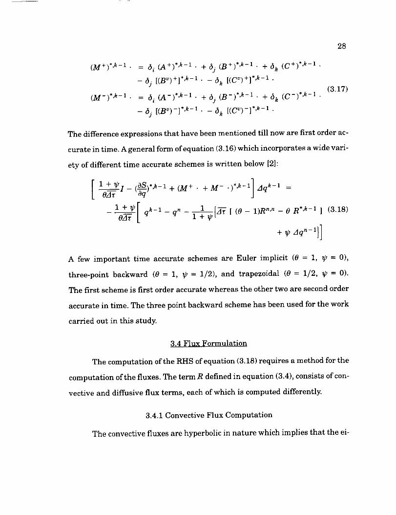
28

(M +)*'k - 1

(M-)*,k- 1 .

= 6 i (A+) *'h-1 • + (_j (B+) *'k-l" + 5 k (C+) *,h-1

- dj [(BY)+] *'k-1 • - 5 k [(CV)+] *'k-1 "

= d i (A-) *'k-l- + dj (B-) *'k-1 • + d k (C-) *'k-l"

-- (_j [(BV)-l*'k-1 " -- (_k [(CV)-]*'k-1 "

(3.17)

The difference expressions that have been mentioned till now are first order ac-

curate in time. A general form of equation (3.16) which incorporates a wide vari-

ety of different time accurate schemes is written below [2]:

1 + _ I - (c)S,) *,k-1OAr "-_" + (M+ "

I"

1 + _0[ qk-1 _ qno-J; I_

1

M- • )*,k- lJ Aqk- 1 =+

1 {A_ [ (0 - 1)R n'n - 0 R *,k-1 ]1+_

+ _ Aqn-1}]

(3.18)

A few important time accurate schemes are Euler implicit (0 = 1, _0 = 0),

three-point backward (0 = 1, _ = 1/2), and trapezoidal (0 = 1/2, _ = 0).

The first scheme is first order accurate whereas the other two are second order

accurate in time. The three point backward scheme has been used for the work

carried out in this study.

3.4 Flux Formulation

The computation of the RHS of equation (3.18) requires a method for the

computation of the fluxes. The term R defined in equation (3.4), consists of con-

vective and diffusive flux terms, each of which is computed differently.

3.4.1 Convective Flux Computation

The convective fluxes are hyperbolic in nature which implies that the ei-

29

genvalues associatedwith the flux Jacobians are real. Thus, there is a preferred

direction of information propagation in such systems. Thus, to be consistent

with the physics of the problem one needs to use the method of upwinding to

evaluate the convective fluxes. Onesuch method is Roe'sflux formulation which

is aflux difference split scheme [12]. The method entails solving an approximate

Riemann problem exactly at each cell face. However, Roe'smethod is first order

accurate in space which is too dissipative for simulation of realistic problems.

Higher order accuracy is obtained by adding corrective flux terms with limiters

[2]. The limiters act as a switching mechanism to control the addition of the cor-

rective flux terms such that the formulation is higher order in smooth regions.

In regions containing shocks or contact discontinuities the formulation is first

order accurate becausein such regions higher order schemesare dispersive. The

limiters used in the corrective flux terms are Roe's Superebee, van Leer's and

minmod limiters. The detailed development of the above formulation is pres-

ented in [13], [14], and [15].

3.4.2 Diffusive Flux Computation

The evaluation of the diffusive fluxes defined in (2.45) requires the nu-

merical representation of derivatives needed for the stress calculations which

can be noted in equations (2.47) and (2.48). The metric terms such as _x, _y,....,

are also needed instead of J_x, J_y, .... , which are the projections of the face

areas in the Cartesian directions and are computed in the code. The diffusive

fluxes are parabolic in nature so that there is no preferred direction of informa-

tion propagation for systems. Thus, the central differencing scheme is the most

popular and easiest way to compute the derivatives appearing in the diffusive

30

fluxes [2]. The implementation of the aboveapproach is illustrated by consider-

ing an example stress term, rxx:

_ 1 2 Ou_ Ov-kz_rxx - _ee'_/x 2kx-_ ky

The following numerical formulae are used to calculate the various terms that

appear in the above equation:

( Jk, ( Jky )k 1( kx )k 1 = )k+½ ( ky = +_ .... (3.19)

+_ ½( Jk + Jk+a )' )k+_ ½( Jk + Jk+l )'

OU OV

('_ )k i = uk+l - uk , ('_ )k+½ = vk+l -- Vk , .... (3.20)+_

The central difference scheme in equation (3.20) is of second order accuracy.

3.4.3 Turbulence Modeling

Equation (2.42), which is the thin-layer Navier-Stokes equation, becomes

Reynolds-averaged thin-layer Navier-Stokes equation which is the time aver-

aged Navier-Stokes equation for turbulent flows, when _ is written as:

/_ = /xz + _t (3.21)

Similarly the thermal conductivity is written as:

k = k l + k t (3.22)

k - /_ _ /Q + /_t (3.23)Pr (y - 1) Pr/ (_ - 1) Pr t (y - 1)

or

where Pr/ = 0.72 and Pr t = 0.90 for air [2].

The Baldwin and Lomax turbulence model [16] is used in this study for

the calculation of/x t. A detailed description of the model is given in [2]. This mod-

31

el is a two-layer algebraic eddy viscosity model in which _tt is evaluated differ-

ently for the inner and outer layers. Since there is no clear demarcation between

the inner and outer layers, _t t at each cell face is calculated by both methods and

then the smaller value is chosen [2].

3.5 The N-Pass Scheme

Equation (3.18) can be written in the general form as:

(L + D + U)X = b (3.24)

where L is strictly lower block triangular, D is block diagonal and U is strictly

upper block triangular. The system of equations defined above can be solved us-

ing the "N-Pass" algorithm. The "N-Pass" algorithm can be viewed as a relax-

ation scheme based on the symmetric Gauss-Siedel algorithm [17]:

L x2N-X

(L + D)X1 + UX° = b }LX 1 + (D + U)X 2 = b

(L + D )+X_-I(D + +U)X_UX _-2__ =b b } N_ pass

i st pass

(3.25)

The nature of L, D, and U can be exploited to reduce the number of matrix vector

multiplications needed to be carried out [7]. The modified two-pass scheme can

be shown to be equivalent to one pass of the "N-Pass" scheme described above.

This has been illustrated by considering a representative one-dimensional sten-

cil in [2]. Since, more than two iterations are needed for the Gauss-Siedel itera-

tive method to yield a converged solution, the "N-Pass" scheme allows the scope

for a more accurate and stable solver. This is so, because with each additional

32

pass one can add two additional Gauss-Siedel iterations, which gives a better

solution. In this study, only one passhas been used to obtain the solution. This

schemehas also beenvectorized using the diagonal plane processing developed

in [13] and [10].

3.6 Boundary_ Conditions

The characteristic variable boundary conditions as applied to the non-

conservative vector form of the transformed Euler equations with source terms

developed in [18] is used in this study. For the viscous computations, at the

walls, the adiabatic wall, no-slip boundary condition developed in [14] is ap-

plied. The inflow boundary condition that is developed in [2] which specifies the

reservoir conditions for internal flows, called the total-condition-preserved

boundary condition does not change between the two formulations. This is so be-

cause inflow is assumed to be uniform at the grid entrance and only in the x-

direction which is normal to the plane of rotation. The only difference in the

boundary conditions that is made when one changes from the fixed frame ap-

proach to the rotating frame approach arises in the subsonic outflow boundary

conditions. The subsonic outflow boundary conditions with source terms are

coupled with the simple radial equilibrium equation described in [19]. The sim-

ple radial equilibrium accounts for the swirl produced downstream of the blades

[21.

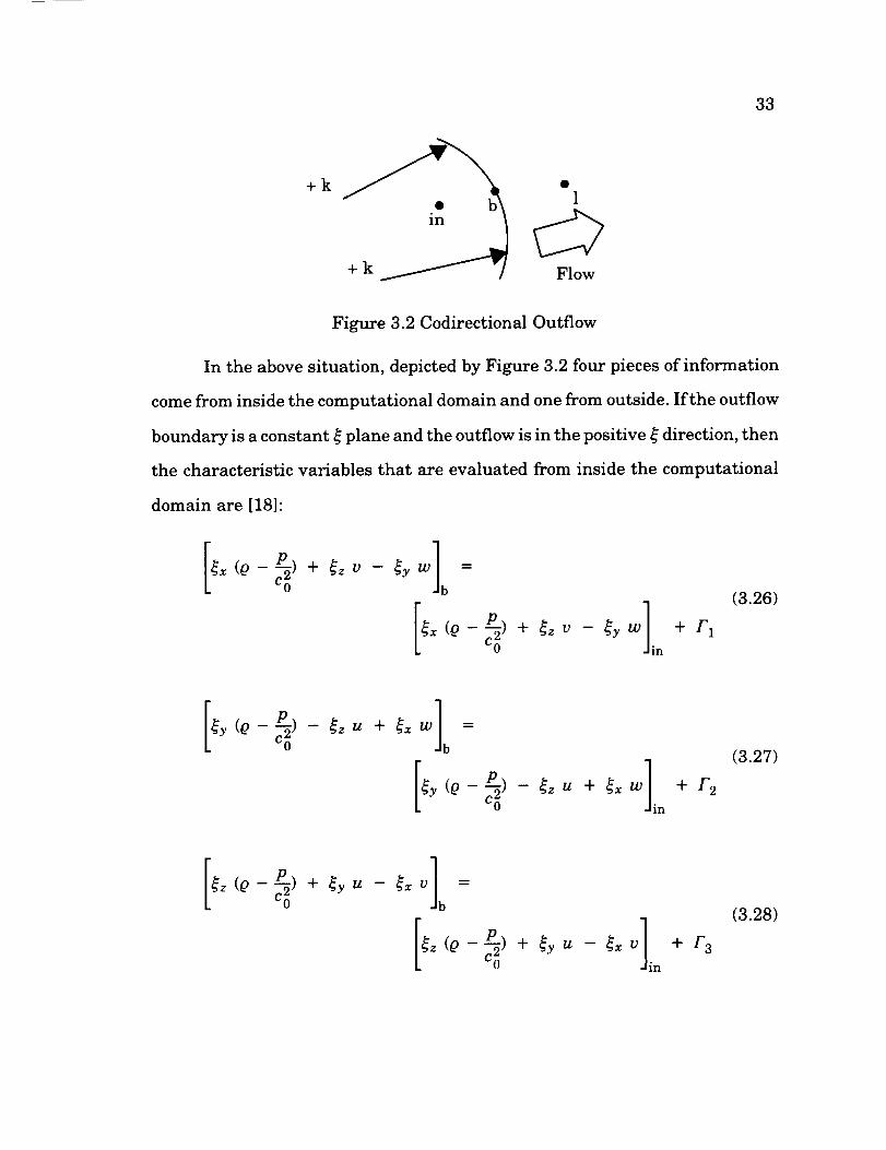
3.6.1 Subsonic Outflow

Subsonic outflow condition is illustrated by the figure below.

33

+k • 1

Figure 3.2 Codirectional Outflow

In the above situation, depicted by Figure 3.2 four pieces of information

come from inside the computational domain and one from outside. If the outflow

boundary is a constant _ plane and the outflow is in the positive _ direction, then

the characteristic variables that are evaluated from inside the computational

domain are [18]:

V-_y w]b=

[_x- P--) + _z(Q]

- _yw / +V

J in

(3.26)

F1

[_y --P---') -- _z + _x W] =

"1

(Q U

c_ .,b

P--) - _zCy (O - C2

]+ _xW I +U

I in

(3.27)

r2

[_z (Q _y UL) +

-_xv] =b

_z (q - P-P-)+_ U m

_x Vii n+r3

(3.28)

+ _yV

plV l

+ zw] =b

+ _x u + _y v

34

(3.29)

where F i = AT IV_ I F_ F = P- 1 M- 1 S. The subscript "0" denotes thatj , _,o

the matrix P_-1 is considered to be locally constant. The P_-1 and M-1 are

derived in [8] and S is defined in (2.46) so that one can write the elements off

as:

F 1 = AT [-- _z W Q -- _y V Q]

1" 2 = A'_ [_x v $"_]

['3 = A Z" [_x w Q]

/'4 = A Z" [-_y w _ q- _z v .(2]

(3.30)

By constructing the grid such that the outflow boundary is normal to the x axis,

the metrics _y and _z will be zero [19]. Utilizing this result in equations

(3.26)-(3.30), the characteristic variables simplify to:

(3.31)

V b ---- Vin -- AT Wav .(-2 (3.32)

W b ---- Win + AT Vav _) (3.33)

+u) +u)b in

where Oo and c o are reference quantities, ray and Way are calculated using

phantom points which are explained later in this section. The calculation of

35

pressure at the outflow boundary is carried out by using the result from the first

three equations above in the radial equilibrium equation [19]:

Orb

(3.35)

A first order finite difference scheme is used to evaluate the derivative and the

right hand side is calculated as the average of the quantity at the two points be-

ing considered. This procedure will yield the following algebraic equation:

rc , ) 1P2-Pl _ 1 \ 7°_ + al v21 _ + a2

r2 - rl 2 ] rl + r2 ] (3.36)[

0- P] and the subscripts 1 and 2 denote the points along thewhere a = _00 in

spanwise direction. Letting f -a v 2

v2 and g - r

c 2 rone gets the following ex-

pression:

P2

Pl + (r2-rl)(= 2 Plfl + gl + g2 ) (3.37)

1 ( r2-rl2 )-f2

The calculation proceeds from the casing (maximum value of r), where the pres-

sure is taken to be the specified back pressure, to the hub. Once the pressure at

the boundary is determined, the density and u can be calculated from the equa-

tions (3.31) and (3.34) respectively.

To implement the boundary conditions a layer of phantom points just out-

side the computational domain is used. The conditions at these points are deter-

36

mined by the following relations:

_p = 2_b - Win (3.38)

where _ is any of the primitive variables and subscript p denotes a phantom

point. Once the primitive variables are determined, the conservative variables

can be calculated at the phantom points. Using the above definition,

Vav and Wav appearing in equations (3.32) and (3.33) can be written as:

Vin 4- VpVa v -- 2

Win 4- WpWav -- 2

(3.39)

It should be noted that Vp and Wp in equation (3.39) are calculated using the

solution at the previous time step.

CHAPTER IV

RESULTS

The aim of the work carried out in this study is to show that, for turboma-

chinery applications, solving the Navier-Stokes equation cast in the rotating

frame has a significant advantage over solving the same in fixed coordinates.

However, one has besure that the change in formulation doesnot introduce any

additional inaccuracy which will degrade the solution. The test casechosen in

this study to validate the formulation is NASA's Rotor 67, which has one row of

rotating blades.

All the computations were performed on the SGI Challenge 10000 XL

computer. The calculations have been carried out with third order spatial and

second order temporal accuracy. The higher order computations and viscous

computations are delayed for a few cycles.

4,1 Rotor 67

The first stage rotor of a NASA Lewis designed two-stage fan, Rotor 67,

has been used to validate the code for a single-rotating geometry in internal flow.

The test case is a low-aspect-ratio, damperless, transonic axial-flow fan rotor.

It has 22 blades of multiple-circular-arc design and no inlet guide vanes. The

inlet relative Mach number at the rotor tip was 1.38 at the designed tip speed

of 428.9 m]sec (16,043 rpm). The designed pressure ratio for the rotor is 1.63 at

a mass flow rate of 33.25 Kg/sec [2].

37

38

The grid used for the computations is very coarse.An H-type grid for the

whole computational domain was generated by TIGER, an interactive turboma-

chinery grid generation code developed by Shih [20]. The grid has dimensions

of 55x31x25 with twenty one points on the blade axially and twenty six points

in the spanwise direction. There is a gap clearance between the blade tip and

the casing. Since this case is at zero angle of attack, only one blade passage

needs to be simulated by taking advantage of the symmetry.

Total-condition-preserved B.C. is used to apply constant uniform condi-

tions at the upstream boundary. Axisymmetric B.C.s are used for re-entry

boundaries. No-slip B.C.s are used on the blades, hub and casing. At the exit

plane, the radial equilibrium boundary conditions with the sourceterms are ap-

plied with the back pressure specified at the radial location corresponding to the

casing. The Reynolds number based on the tip diameter at the designed speed

and standard day conditions was about 8,000,000.

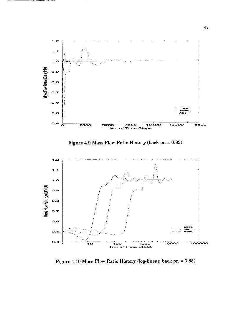
The solution is considered converged when the following are true:

1. The inlet massflow rate changedless than 0.2%of the average of the max-imum and minimum values in 1000 cycles.

2. Mass flow ratio (outlet ! inlet) varied between 1 + 0.005 in 1000 cycles.

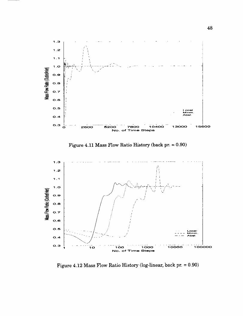
For the above test case three conditions were run with the non-dimen-

sional back pressures of 0.75, 0.85, and 0.90 which correspond to choke, near

peak efficiency and near stall conditions respectively. Since the problem can be

viewed as a steady state flow in the rotating frame, the relative frame code is run

with both, local time stepping and minimum time stepping. The absolute frame

code can only be run with minimum time stepping. Figures 4.1, 4.3, and 4.5 show

39

a comparison of mass flow histories between the relative frame and the absolute

frame codes,for the three conditions, respectively. The comparison of the behav-

ior of the mass flow ratio is presented in Figures 4.7, 4.9, and 4.11.

As can beobserved from the mass flow histories, the absolute frame code

requires a much longer time to yield a satisfactorily converged solution. The ab-

solute code was run with a CFL=70 which corresponds to 2600 time steps per

revolution, and with 2 Newton sub-iterations per time step. When using local

time stepping the rotating frame codewas run with a CFL=50; no Newton sub-

iterations. While using minimum time stepping the relative code was run with

a CFL=10000, corresponding to 18 time steps per revolution. However, the ini-

tial 400 cycleswere run with a CFL=500. Thereafter, the CFL was increased to

10000.

The absolute coderequires 10400 cycles (4 revolutions) to produce a con-

verged solution, whereas the rotating frame code requires a minimum of 1500

cycles to give a converged solution when run using minimum time stepping.

When local time stepping was used, a minimum of 1500 cycles were needed.

Thus, there is no significant advantage of using the local time stepping method

with the rotating frame code. This can be attributed to the very high CFL that

can be used when running with the minimum time stepping method. It can be

observed from the plots that as the back pressure is increased progressively,

more number of cycles are required to obtain a converged solution. The final in-

let mass flow rates between the two formulations varies by less than + 1%. The

advantage can be better appreciated on a semi-log plot which has been shown

in Figures 4.2, 4.4, and 4.6 for inlet mass flow and Figures 4.8, 4.10, and 4.12

40

for mass flow ratio. Another observation that canbe made from the plots is that

the mass flow ratio settles down much faster than the inlet mass flow for all the

three cases.

The speedup that one observes due to the above description is huge. The

absolute frame coderequires 38 hours of running time to complete one revolu-

tion, whereas the relative frame code requires 10 hours running time for 2000

cycleson an SGI Challenge 10000XL. The CPU times required by the two for-

mulations for the three different conditions are illustrated in the table below.

Since there was no difference in the number of cycles required with the relative

frame formulation when using local time stepping or minimum time stepping,

the CPU times corresponding to the relative method using both approaches is

the same.

Table 4.1

Performance Enhancement

METHOD

RELATIVE

ABSOLUTE

TIME(hrs.)

back pr. = 0.75

7.5

TIME

(hrs.)

back pr. = 0.85

12.5

152 171

TIME

(hrs.)

back pr. = 0.90

15

190

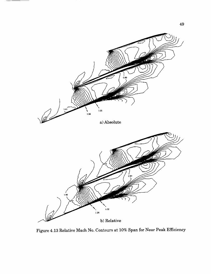
In order to ensure the accuracy of the solution, a comparison is made be-

tween the relative Mach number contours obtained from by solving the two for-

41

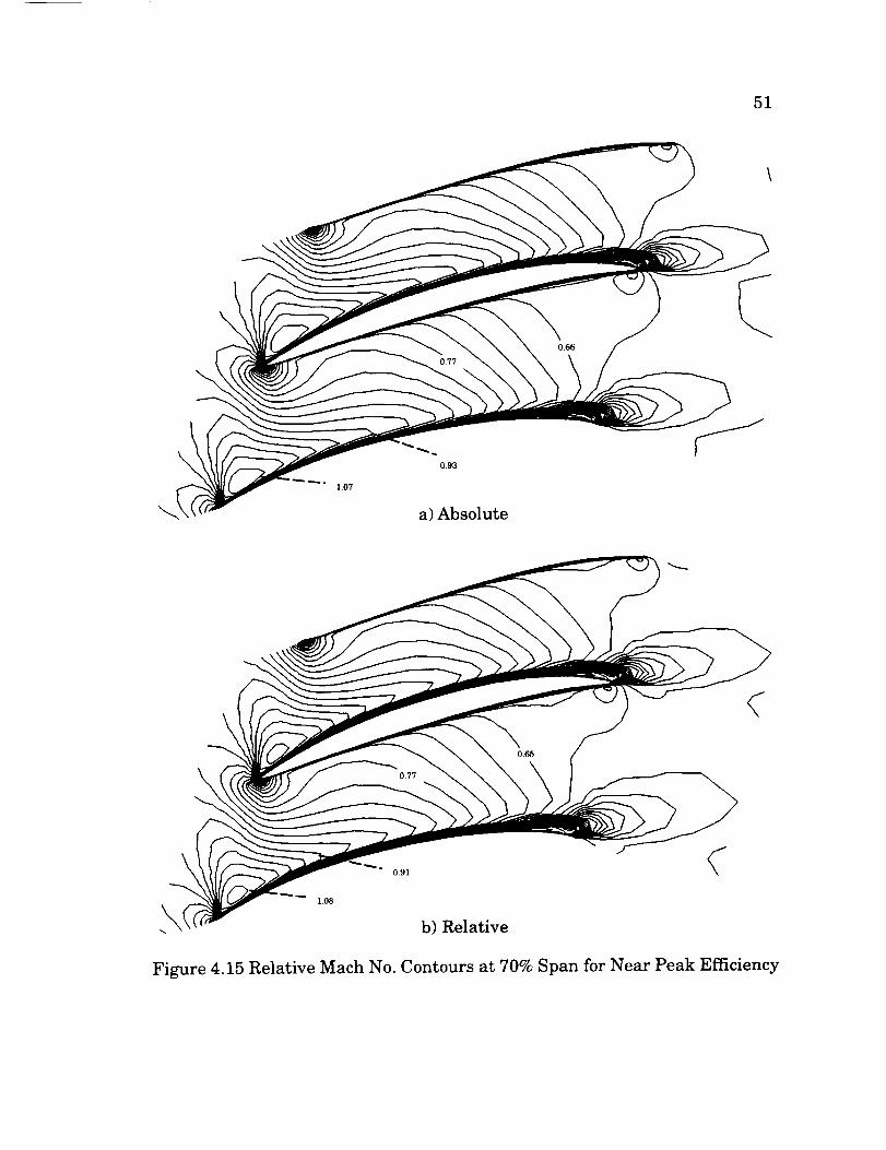
mulations. The comparisons are made at two operating points, one near peak

efficiency and the other near stall condition, and at 10%, 30%, and 70% span

locations from the blade tip. The operating point near peak efficiency occurs at

a non-dimensional back pressure of 0.85 which results in an inlet mass flow of

33.89 kg/sec, which is 97.86% of the computed choked flow, which occurs at a

non-dimensional back pressure of 0.75.For the sameback pressure the absolute

frame codehas amass flow rate which is 98.39% of the choked flow rate. Figures

4.13-4.15 illustrate the comparisons for this operating point and for 10%,30%,

and 70% spanwise locations respectively.

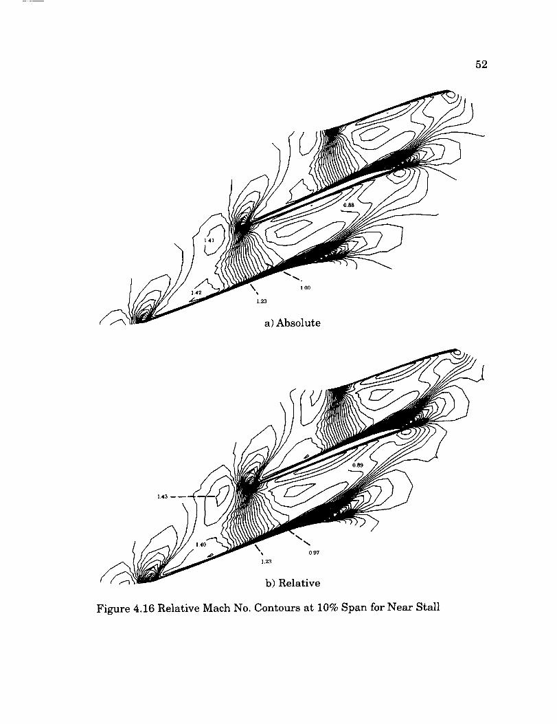
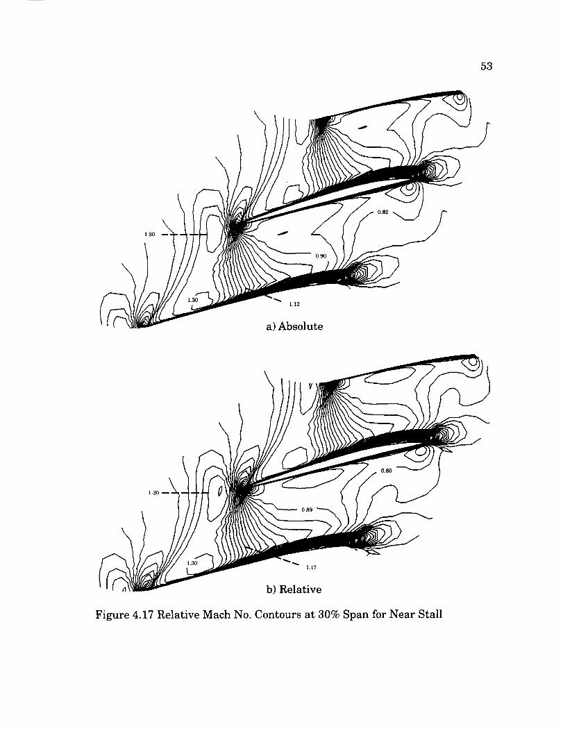
The near stall condition occurs at a non-dimensionless pressure of 0.90.

The relative frame codeyields an inlet mass flow rate of 32.49 kg/sec which is

93.82% of the computed choked flow rate, for this condition. The absolute frame

yields an inlet mass flow rate which is 94.91%of the choked flow rate. The rela-

tive Mach number contours for this condition at the various spanwise locations

are shown in Figures 4.16-4.18.

It can be observed from the figures that there is a good agreement be-

tween the relative Mach number contours. Thus, it can be concluded that the

formulation presented in this study does not introduce any additional errors.

The discrepancies between the computed relative Mach number contour plots

and the experimental plots are the same for the two formulations and are not

discussed in this work.

A detailed description of the flow field and the agreement and discrepan-

cies between computed and experimental results is given in [2]. Another ob-

servation that was made during the course of this study is that the relative

42

frame codedoesproduce a converged solution for a non-dimensional back pres-

sure of 0.95 whereas the absolute frame code exhibits a stall condition beyond

a non-dimensional back pressure 0.90.

43

35.5

35.0

34.5

34.0

33.5

33.0

/

, 1 I /

!p _ i _

: i i /1

p _ !

J _ j'

i

p

i

_ ft _

lj' '_,/r"

\, /. I

Loclll

.... Mlnm.

-- - -- Ablll.

0 2600 5200 7800 10400

No. of Time Steps

33000 15600

Figure 4.1 Mass Flow History (back pr. = 0.75)

35.5 ....... _ ........ • ........ _ ........ , ........

35.0

34.5

34.0

33.5

33.0

i /

i t

i'

,j

• /f "_,

• / ,

....... -i'o

Locl_l

Mlnm.

Abel.

..... loo ..... -__5'oo .... -__,',hoo- " :I"0_,oooNo. of Time Steps

Figure 4.2 Mass Flow History (log-linear, back pr. = 0.75)

44

_E

35.5

35.0

34.5

34.0

33.5

33.0

32.5

32.0

31 .5

31 .0

30.5

30.0

29.5

i

:i ,' r

i

i'

i

i

I

I'

I

i

I

I

I

i

LOGS!

.... MInm.

-- - -- Ab81.

0 2600 5200 7800 10400

No. of Time Steps

33000 35800


35.5

35.0

34.5

34.0

33.5

33.0

32.5

32.0

31 .5

31 .0

30.5

30.0

29.5

Local

Mlnm.

Abel.

10 1 O0 1000 10000 100000

NO. of Time Steps


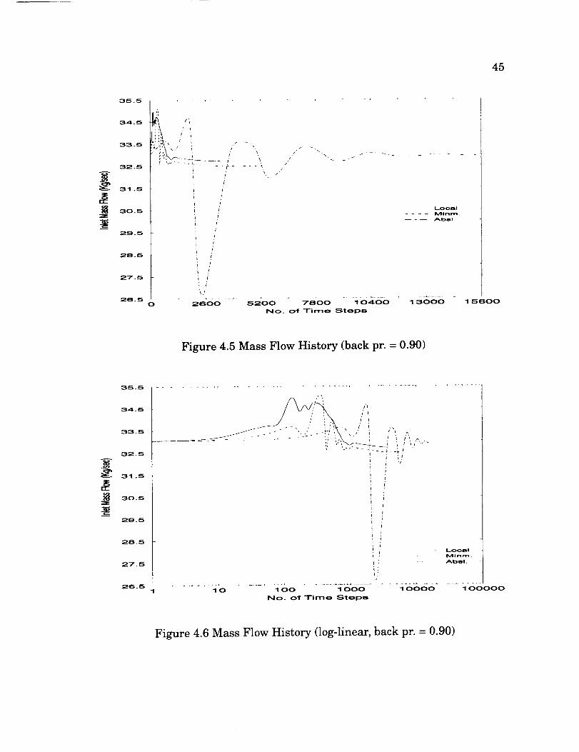
45

35.5

34.5

33.5

32.5

31 .5

30.5

29.5

28.5

27.5

26.5

' [.

' i

x, /,J .\

/

I

!I

f

i

!

/

I

J

o

/

Local

.... Mlnm.

-- - -- Abel.

2600 5200 78'00 " 10400 " 13()00

NO. of Time Steps

15600


35.5

34.5

33.5

32.5

31 .5

30.5

29.5

28.5

27.5

26.5

," ',

¢' L

.j

I

t

i

i

t J

Local

Mlnm.

Abel.

1 o 1oo 1 ooo 10000" 1"ooooo\ S_

No. of Time Steps


46

1.1

1.O

O.9

O.8

O.7

O.8

O.5

Local

.... Mlnm.

-- - -- Absl.

o 2800 5200 7800 10400 13000

No. of Time Steps

15600

Figure 4.7 Mass Flow Ratio History (back pr. = 0.75)

1.1

1.O

O.9

0.8

0.7

0.6

0.5

Local

Mlnm.

Abel.

10 1 O0 1000 10000 100000

No. of Time Steps

Figure 4.8 Mass Flow Ratio History (log-linear, back pr. = 0.75)

47

1.2

1.1

1.0

0.6

0.7

0.6

0.5

0.4

! '1

!! \ ,!

LocalMlnm.Abel.

0 2600 5200 7800 10400 13000

NO. of Time Steps

15600


1.2

1.1

1.0

0.9

0.8

0.7

0.6

0.5

0.4

,," ',. . ! i

/-/ U i,' /" _ /

" r'

, ir

/ j

_ ' t' -- -- Local

............... 4oo 1 ooo 1 oooo 1 ooooo1 10

No. of Time Steps


48

o

:=E

1.3

1.2

1.1

1.0

o.g'

0.6

0.7

0.6

0.5

0.4

0.3

i ._.

sr ,

- j

i

I

. /.\

0 2600 5200 7800 10400

NO. of Time Steps

Local

MInm.

Absl.

± =

13000 15600


1.3

1.2

1.1

1.0

0.9

0.6

0.7

0.6

0.5

0.4

0.3

Local

MInm.

Abel _

................. -ioo ............... 4o_oo" " " :_00ooo10 1000

No. of Time Steps


49

1.26

\

1.05

a) Absolute

1 40

b) Relative

Figure 4.13 Relative Mach No. Contours at 10% Span for Near Peak Efficiency

5O

I.i0

I 1.25a) Absolute

1.02

C1.10

\

1.22 b) Relative


51

\

0.77

0.66

\

1.07

0.93

a) Absolute

\0.77

0.65

0.91

1.08

k,__" b) Relative


52

a)Absolute

1,43

?

\

1.23

0.97

b) Relative

Figure 4.16 Relative Mach No. Contours at 10% Span for Near Stall

53

1.30

0.90

0.82

1,12

a) Absolute

1.30

0.89

0.80

1.17

b) Relative


54

\

0.72

0.62

\

\

1.07

0,87

a) Absolute

\

\0_70

0.61

1.05

0.87

b) Relative


CHAPTER V

SUMMARY AND CONCLUSIONS

The results presented in Chapter IV amply demonstrated that solving the

Navier-Stokes equations in rotating coordinates is a worthwhile exercise and

provides a huge advantage in terms of savings in computer time. The savings

are due to two main advantages of the rotating frame approach over the inertial

frame approach. Since the flow can be considered to be steady in the rotating

frame, noNewton sub-iterations are required sothat less computing time is re-

quired for each time step. This is augmented by the improved stability of the ro-

tating frame codewhich allows it to handle a far larger CFL than the absolute

frame code.This reduces the total number of cycles that are needed to obtain a

converged solution. Also the need to move the grid is obviated due to which the

metric terms do not needrecomputing after eachtime step. All the abovefactors

contribute to the huge savings in computing time. The speedup in CPU time ob-

tained for the test casein this study was a factor of 16. Moreover, the approach

used in this study did not utilize multigrid method or Jacobian freezing. These

two factors can contribute to further savings in computing time.

The enhancement in the performance of the codeis achieved by making

a few minor modifications to the codeto incorporate the rotating frame formula-

tion. To summarize, they are the following:

1. Freezing of the grid motion.

2. Calculating the term kt, analytically as described in Chapter II.

55

56

3. Addition of the source term implicitly in the flux balance.

4. Addition of the source term in the subsonic outflow CVBC which iscoupled with the radial equilibrium equation.

The results presented for the test caseshow that the solution obtained by

the relative frame formulation is in very good agreement with the results ob-

tained with the relative frame formulation. The significant improvement in sta-

bility is useful for problems with different time scales in turbomachinery com-

putation. Since the rotating frame formulation freezes the frequency associated

with the grid rotation, the time scalesassociatedwith other frequency (e.g.blade

fluttering ) canbeused to investigate the unsteady behavior related to that par-

ticular time scale.Thus, it canbeconcluded that this approach is the right direc-

tion to take for simulation of flows through turbomachinery, which can be

treated as steady state problems in the rotating frame.

Future work will entail implementing the relative frame formulation for

a multi-blade row configuration to simulate the flow through a stage. However,

this would involve transformation of the dependant variable vector between the

fixed and rotating frames before exchanging information between blade rows.

Addition of the multigrid method and parallelization of the code are two other

areas of future work.

REFERENCES

[1]

[21

[3]

[4]

[51

[61

[71

[81

[91

[10]

Adamcyzk, J.J., "Model Equation for Simulating Flows in Multistage

Turbomachinery," ASME Paper No. 85-GT-226, November 1984.

Chen, J.P., "Unsteady Three-Dimensional Thin-Layer Navier-Stokes

Solutions for Turbomachinery in Transonic Flow," Ph.D. Dissertation,

Mississippi State University, Mississippi, December 1991.

Adamczyk, J.J., Celestina, M.L., Beach, T.A., and Barnett, M., "Simula-

tion of Three-Dimensional Viscous Flow Within a Multistage Turbine,"

ASME Journal of Turbomachinery, Vol. 112, No. 3, July 1990. pp.

370-376.

Agarwal, R.K., and Deese, J.E., "Euler Calculations for Flowfield of a He-

licopter Rotor in Hover," McDonnell Douglas Research Laboratories,

MDRL Report 86-10, June 1986.

Chima, R.V., and Yokota, J.W., "Numerical Analysis of Three-Dimension-

al Viscous Internal Flows," AIAA Journal, Vol. 28, No. 5, May 1990. pp.

798-806.

Warsi, Z.U.A., "Fluid Dynamics: Theoretical and Computational Ap-

proaches," CRC Press, Inc., Boca Raton, 1993.

Whitfield, D.L., "Newton-Relaxation Schemes for Nonlinear Hyperbolic

Systems," Engineering and Industrial Research Station Report, MSSU-

EIRS-ASE-90-3, Mississippi State University, Mississippi, October 1990.

Janus, J.M., "The Development of a Three-Dimensional Split Flux Vector

Euler Solver with Dynamic Grid Applications," M. S. Thesis, Mississippi

State University, Mississippi, August 1984. pp. 14-27.

Whitfield, D.L., "Implicit Upwind Finite Volume Scheme for the Three-

Dimensional Euler Equations," Engineering and Industrial Research

Station Report, MSSU-EIRS-ASE-85-1, Mississippi State University,

Mississippi, September 1985.

Belk, D.M., "Three-Dimensional Euler Equations Solutions on Dynamic

Blocked Grids," Ph.D. Dissertation, Mississippi State University, Missis-

sippi, August 1986.

57

[11]

[12]

[13]

[14]

[15]

[16]

[17]

[18]

[19]

[20]

58

Whitfield, D.L., and Taylor, L.K., "Discretized Newton-Relaxation Solu-tion of High Resolution Flux-Difference Split Schemes,"AIAA Paper No.91-1539, June 1991.

Roe,P.L., "Approximate Riemann Solvers, Parameter Vectors, and Differ-ence Schemes,"Journal of Physics, Vol. 43, 1981. pp. 357-372.

Janus, J.M., "Advanced 3-D CFD Algorithm for Turbomachinery," Ph. D.Dissertation, Mississippi State University, Mississippi, May 1989.

Simpson, L.B., "Unsteady Three-Dimensional Thin-Layer Navier-StokesSolutions on Dynamic Blocked Grids," Ph.D. Dissertation, MississippiState University, Mississippi, December 1988.

Whitfield, D.L., Janus, J.M., and Simpson, L.B., "Implicit Finite VolumeHigh Resolution Wave-Split Schemefor Solving the Unsteady Three-Di-mensional Euler and Navier-Stokes Equations on Stationary or DynamicGrids," Engineering and Industrial Research Station Report, MSSU-EIRS-ASE-88-2, Mississippi State University, Mississippi, February,1988.

Baldwin B.S., and Lomax, H., "Thin Layer Approximation and AlgebraicModel for Separated Turbulent Flows," AIAA-78-257, January 1978.

Sreenivas, K., "High Resolution Numerical Simulation of the LinearizedEuler Equations in Conservation Law Form," M. S. Thesis, MississippiState University, Mississippi, July 1993. pp. 30-31.

Kisielewski, K.M., "A Numerical Investigation of Rain Effects on Lift Us-ing aThree-Dimensional Split Flux Vector Form of the Euler Equations,"M. S. Thesis, Mississippi State University, Mississippi, May 1985. pp.29-36.

Whitfield, D.L., Swafford, T. W., Janus, J.M., Mulac, R.A., and Belk, D.M., "Three-Dimensional Unsteady Euler Solutions for Propfans andCounter-Rotating Propfans in Transonic Flow," AIAA-87-1197, June1987.

Shih, M.H., "TIGER: Turbomachinery Interactive Grid genERation,"M.S. Thesis, Mississippi State University, Mississippi, December 1989.

APPENDIX A

DERIVATION OF THE VELOCITY OF THE MOVING COORDINATES

59

6O

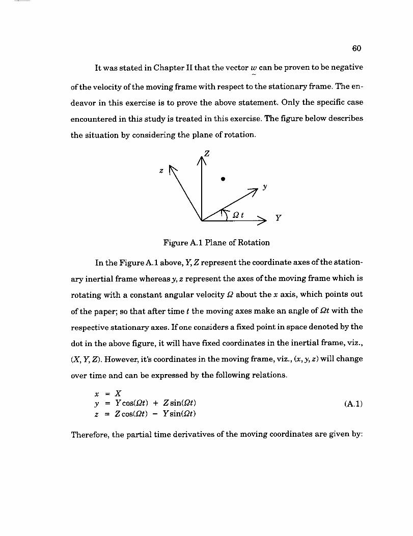
It was stated in Chapter II that the vector w can be proven to be negative

of the velocity of the moving frame with respect to the stationary frame. The en-

deavor in this exercise is to prove the above statement. Only the specific case

encountered in this study is treated in this exercise. The figure below describes

the situation by considering the plane of rotation.

Z

Z

• y

Yf

Figure A. 1 Plane of Rotation

In the Figure A. 1 above, Y, Z represent the coordinate axes of the station-

ary inertial frame whereas y, z represent the axes of the moving frame which is

rotating with a constant angular velocity t2 about the x axis, which points out

of the paper; so that after time t the moving axes make an angle of t2t with the

respective stationary axes. If one considers a fixed point in space denoted by the

dot in the above figure, it will have fixed coordinates in the inertial frame, viz.,

(X, Y, Z). However, it's coordinates in the moving frame, viz., (x, y, z) will change

over time and can be expressed by the following relations.

x =X

y = Ycos(t2t) + Zsin(sgt)

z = Z cos(t2t) - Ysin(_2t)

(A.1)

Therefore, the partial time derivatives of the moving coordinates are given by:

61

OX - 0 (A.2)Ot

_J = f2 [Zcos(Qt) - Ysin(f2t)] = Qz (A.3)Ot

OZ- t2 [Ycos(_t) + Zsin(f2t)] = - f2y (A.4)

dt

The vector w is defined in equation (2.3) as:

w - Oxi a (A.5)_ Ot -i

According to the coordinate system described in Figure A.1,

X 1 = X, X 2 = y, x 3 = z and for simplicity let i, j, and k represent the Car-

tesian base vectors of the moving frame. Thus,

_ Ox Oy. Ozw - -_-fi + _-fj + _-fk = f2zj - Qyk (A.6)

The velocity of the moving frame with respect to the inertial frame is given by:

ijk

f200

xyz

= - t2zj + f2yk (A.7)

It can be observed from equations (A.6) and (A.7) that:

w= -f2X r (A.8)

APPENDIX B

CURVILINEAR COORDINATE TRANSFORMATION OF THE NAVIER-

STOKES EQUATIONS

62

63

The governing equations in conservation law vector form using nondi-

mensional variables in rotating Cartesian coordinates is given by:

Oq Ot Og Oh Ofv + OgV Ohv + s (B.1)o-7 + o-_ + _ + oz - ox -_ + oz

where the vectors q, f, g, h, fv, gV, h v, and s are all defined in equations

(2.17)-(2.20). A general nonorthogonal, steady, curvilinear coordinate system is

introduced in the (x, y, z) space as follows:

= _(x,y,z)

rl = rl(x,y,z)

= _(x,y,z)

z=t

(B.2)

It should be noted that through equations (B.2) the rotating Cartesian coordi-

nates are transformed to rotating curvilinear coordinates. In other words, the

transformation takes place between two coordinate systems within the rotating

frame. Using chain rule and writing the result in matrix form yields:

"0"Ot

0Ox

0

Oy0Oz

'1

0

0

0

000

Cy T]y _y

_z _z _z

"0"Ov0

0

07

0

(B.3)

The inverse transformation in matrix form is:

64

a-_ "1

0-- 0a_0 =

o_ o0

_ 0

This implies that:

"10 0 0"

0 _x _x _x

0 _y _y _y

000"

x¢ y¢ z¢

xv 27 z_

x_ y_ z_

"1

0

0

0

"0"at

0Ox0

oy0Oz

0 0 0"

x¢ y¢ z¢

x_ yn z_

x_ y_ z_

-1

(B.4)

(B.5)

Thus, J, which is the Jacobian of the inverse transformation, can be written as:

J

1 0 0 0

0 x_ y_ z$

0 x, y_ z_

0 x_ y_ z_

x$ y$ z_

= x_ 27 z_

x¢ y¢ z¢(B.6)

= x_(y_z¢- z_y¢) - y_(x_z¢- z_x_) + z_(x_y¢- y_x¢)

The metric terms in equation (B.3) can now be expressed by the following rela-

tions:

_x = l(y_z¢- z_y¢) _/x = l(z_y¢-yCz¢) _x = l(ycz¢- z_y¢)

_y = _(ZtIX_- Xr/Z_) r]y --- _(X_-Z_- Z_X_) Cy --- _(Z_,Xt_- X_Z_/) (B.7)

1 = !/(x_y_

The governing equations in curvilinear coordinates, therefore are:

0-7 + _x (f-if) + rlxo_(f-f _) + _x (f-if)

O(g

Multiplying throughout by J yields the following:

= Js

Using the identity:

J_x_

the equation (B.9) becomes:

-_v(Jq) - q-_ + [J(_xf + _yg + _zh)] + [J(t/xf + tlyg + rlzh)]

+ _[J(_xf + _yg+_zh)]- (f- ff)[_(J_x) + O-_(Jrlx)+ _(J_x)]

0 (jtly) + _(j_y)]_ (g _ gV)[__(j_y) + "_

- (h - hV)[-_-_ (J,z) + O_-_(J_lz) + _(J_z)]

0= 0__[j(_j_ + _yg_ + _zh_)] + -_ [j(_j_ + _yg_ + _zh_)]

+ _ [j(_j_ + _ygV+ _zhV)l+ Js

Since the curvilinear transformation is steady:

65

(B.8)

(B.9)

(B.10)

(B.11)

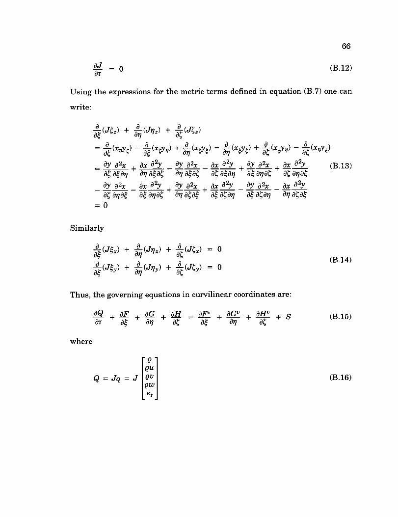
66

OJ - 0 (B.12)0v

Using the expressions for the metric terms defined in equation (B.7) one can

write:

= -_(xny¢)- -_-_(xCy,7)+ _(xCy$) - _(x_y¢) + _(x_y_) - _(x_y$)

_ Oy 02X c_X O2Y Oy 02X c_X 02Y Oy 02X OX O2Y (B.13)

0¢0_07 + o70_0_ o70_0¢ o_0_07 + ot 070¢ + 0¢ 070t

Oy O2x Ox 02Y Oy 02x Ox O2Y Oy 02x OX 02Y+ +

aCaTa_ ata7a_ 07a¢0_ a_aCa7 ataCa7 07aCa_=0

Similarly

O"_-(J_x) + O-_(JTx) + -_(J_x) =0at

0 0 (JTy) + -_(J_y) = 0-_(Jty) + -_

(B.14)

Thus,

where

the governing equations in curvilinear coordinates are:

_ OH voQ OF OG OH OF v OGv + + S (B.15)

Q =Jq =J J (B.16)

m

K= J( kx.f + kyg + kzh )

QK'

_uK' + kxp

= j 9vK' +kyp

_wK' + kzp

etK' + pK

where K' = kxu ÷ kyv ÷ kzw + k t

k t = - kyQz + kz_y

K = kxu + kyv + kzw

67

(B.17)

_v = j(

=J

kxf v + kyg v + kzh v )

"0]

TkyTkzl.QkJ

(B.18)

S =Js =J

0

0

- Ow_2

QvQ

0

(B.19)

In the above equations (B.17) and (B.18), K = F, G, H; K' = U', V', W';

K= U, V, W; _ = F v, G v, HV; for k = _, r/, _ respectively. The trans-

formed viscous stress and heat flux terms in equation (B.18) can be expressed

in terms of the derivatives with respect to curvilinear coordinates by applying

the chain rule to the derivatives appearing in the viscous stress and heat flux

terms of the viscous flux vectors in equation (2.19). The transformed viscous

stress and heat flux terms are defined in detail in equations (2.39)-(2.41).

APPENDIX C

CYLINDRICAL COORDINATE FORMULATION

68

69

The Navier-Stokes equations in cylindrical coordinates, in an absolute

frame with absolute velocity components using non-dimensional variables can

be written as:

oq of 08 oK of + o_ o_o-7 + _ +-_7 + oO - Oz -_- + oO + k (C.1)

where

q=

rQ

rQUz

rQUr

"20U _

re t

(C.2)

f

r_Uz

r(Qu 2 + p)

rOU rU z

r2OUoUz

roHuz

, g----

rQUr '

rQUzUr

.(eU2r+ p)

r2oUoUr

rQHu r

M

h=

QU 0

OUzU 0

OUrU o

r(ou 2 + p)

QHu e

(C.3)

[rTOz] [rTOr] [TzO1

F ---- /rr_r'Zoz/ ' g-V ---- /rr_;r I' h-V -- ['/'rOlrvO0[ rqz j [ rqr J qo

(C.4)

k=

q

0 i0

2u_ + 0p - _°° I

02

(C.5)

7O

In the above equations Uz, Ur, and u 0 are the axial, radial, and tangential ab-

solute velocity components respectively, e tP

1 2 u 2 + Uo2) and+ -_O(Uz +

H - et + p Also,"

TOO--2/_

3 Re

20Uz OUr IOUo UrOz Or r O0 r

2 OUr 10Uo OUz UrOr r O0 Oz r

"20Uo OUz OUr Urr O0 Oz Or + 2--y-

[OUz OUr]_zr -_ Tr-z = Re [ Or + Oz J

_ _ [I_OUr OUo

VrO = "gOr Re [ r O0 + Or

. [ouo lOU 1VOz = VzO = R'e[ Oz + r OOJ

(C.6)

qz = VzzUz + 7JzrUr -4- _'zOUO + _ee

qr = VrzUz + VrrUr + VrOU 0 + _ee

qo = %zUz + VorUr + vOOUo + R_e

/u aT

(y- 1)Pr az

ju aT

(_, - 1)Pr Or

/_ ]lOT(?, - 1)Pr ?" O0

(C.7)

For flows in a rotating frame, equation (C.1) can be cast in the relative

(rotating) frame by the transformation [3]:

Oab s ---- Ore1 - _t (C.8)

where Q is the rotational speed (negative with 0). Introducing equation (C.8)

into equation (C.1) yields:

71

Oq Of Og O(h+ ..Qq) O/W 0_' + oh-¢' + _ (C.9)o-7 + az +-_7 + o0 - az + 0--7- aO

The above equation is in cylindrical coordinates but in the rotating frame. How-

ever, the velocity components in equation (C.9) are the components of the abso-

lute velocity, the only difference being that the components are now expressed

in the relative frame. If one introduces a transformation in the relative frame,

from the cylindrical (z, r,

nates which is of the form:

X -_ z

Y = rcos0

Z = rsin0

0) coordinates to the Cartesian (X, Y, Z) coordi-

(C.10)

equation (2.16) can be derived by repeating the procedure discussed in Appen-

dix A. Using chain rule and writing the result in matrix form yields:

"0"Ot

0Oz

0Or0

oO. •

"1000

0100

0 0 YrZr

0 0 YoZo

0'

Ot0

oX0

OY

0OZ

(C.11)

The inverse transformation in matrix form is:

"0

Ot0

0

aY

0O2

'1

0

0

0

0 0 0

100

0 ry r Z

00yO z

"0"

Ot0

Oz

0Or

0O0

. •

From equation (C. 10) the following results can be derived:

(C.12)

72

Yr = cos 0, Y0 = - r sin 0, Zr = sin 0, Z 0 = r cos 0

ry = cos0, r Z = sin0, Oy _ Sinr0, Oz _ COSr0(C.13)

Thus, the Jacobian of the inverse transformation is given by:

1 (C.14)J = ryO z - rzO Y -- -_

Also, the following relations hold between the components of the absolute veloc-

ity vector in the two coordinate systems

U X -'-- U -_ Uz

Uy = v = UrCOSO - u6sin0 (C.15)

u z = w = UrsinO + uecos0

Although, in the present context, the above relations give the relation between

the components of the absolute velocity, it must be mentioned that they are valid

for the components of any vector in the two coordinate systems. Applying the

chain rule to equation (C.9) and using the relations derived above, yields the fol-

lowing form of the equations:

Oq Of Og Oh Ofv Og v Oh v0-_ + -_ + -_ + OZ - OX + --OY + OZ + s (C.16)

where

q(C.17)

73

f

Qu

Qu 2 -I- p

Ouv

Ouw

u(e t + p)

g

Qv - QI2z

Ovu - Out2z

Qv 2 + p - OvI2z

Ovw - Owt2z

v(e t + p) -- et.Qz

I ° lTxx

Vxy

Txz

rxx + Vrxy + Wrxz + qx

Ow + O_2y

Owu + Out2y

Owv + ovi2y

?W 2 + p + Owi2y

w(e t + p) + efl2y

(C.18)

gU __

0

ry_

ryy

Tyz

+ Vryy + WVyz + qy

(C.19)

h v 0 1Tzx

Tzy

Tzz

4- I)'t'zy 4- WVzz 4-qz

S

0

0

- pw_

Ova2

0

(C.20)

It can be observed from the above equations (C.17)-(C.20) that the equations in

Cartesian coordinates derived via the cylindrical coordinates are identical to

equation (2.16).

SOLUTIONS TO THREE-DIMENSIONAL THIN-LAYER … · solutions to three-dimensional thin-layer...

Documents

Transcript of SOLUTIONS TO THREE-DIMENSIONAL THIN-LAYER … · solutions to three-dimensional thin-layer...