Solutions of differential equations using transformskglasner/math456/FOURIER2.pdf · Solutions of...
52
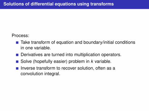
Solutions of differential equations using transforms Process: Take transform of equation and boundary/initial conditions in one variable. Derivatives are turned into multiplication operators. Solve (hopefully easier) problem in k variable. Inverse transform to recover solution, often as a convolution integral.
Transcript of Solutions of differential equations using transformskglasner/math456/FOURIER2.pdf · Solutions of...
Solutions of differential equations using transforms
Process:Take transform of equation and boundary/initial conditionsin one variable.Derivatives are turned into multiplication operators.Solve (hopefully easier) problem in k variable.Inverse transform to recover solution, often as aconvolution integral.
Ordinary differential equations: example 1
− u′′ + u = f (x), lim|x |→∞
u(x) = 0.
Transform using the derivative rule, giving
k2u(k) + u(k) = f (k).
Just an algebraic equation, whose solution is
u(k) =f (k)
1 + k2 .
Inverse transform of product of f (k) and 1/(1 + k2) isconvolution:
u(x) = f (x) ∗(
11 + k2
)∨=
12
∫ ∞−∞
e−|x−y |f (y)dy .
But where was far field condition used?

Ordinary differential equations: example 2
Example 2. The Airy equation is
u′′ − xu = 0, lim|x |→∞
u(x) = 0.
Transform leads to
−k2u(k)− i u′(k) = 0.
Solve by separation of variables: du/u = ik2dk integrates to
u(k) = Ceik3/3.
Inverse transform is
u(x) =C2π
∫ ∞−∞
exp(i[kx + k3/3])dk .
With the choice C = 1 get the Airy function.
Partial differential equations, example 1
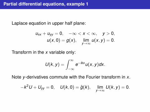
Laplace equation in upper half plane:
uxx + uyy = 0, −∞ < x <∞, y > 0,u(x ,0) = g(x), lim
y→∞u(x , y) = 0.
Transform in the x variable only:
U(k , y) =∫ ∞−∞
e−ikxu(x , y)dx .
Note y -derivatives commute with the Fourier transform in x .
−k2U + Uyy = 0, U(k ,0) = g(k), limy→∞
U(k , y) = 0.
Partial differential equations, example 1
Laplace equation in upper half plane:
uxx + uyy = 0, −∞ < x <∞, y > 0,u(x ,0) = g(x), lim
y→∞u(x , y) = 0.
Transform in the x variable only:
U(k , y) =∫ ∞−∞
e−ikxu(x , y)dx .
Note y -derivatives commute with the Fourier transform in x .
−k2U + Uyy = 0, U(k ,0) = g(k), limy→∞
U(k , y) = 0.

Partial differential equations, example 1, cont.
Now solve ODEs
−k2U + Uyy = 0, U(k ,0) = g(k), limy→∞
U(k , y) = 0.
General solution is U = c1(k)e+|k |y + c2(k)e−|k |y . Usingboundary conditions,
U(k , y) = g(k)e−|k |y .
Inverse transform using convolution and exponential formulas
u(x , y) =g(x) ∗(
e−|k |y)∨
= g(x) ∗(
yπ(x2 + y2)
)=
1π
∫ ∞−∞
yg(x0)
(x − x0)2 + y2 dx0.
Same formula as obtained by Green’s function methods!
Partial differential equations, example 2
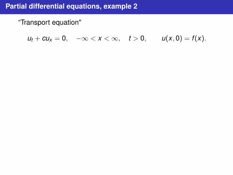
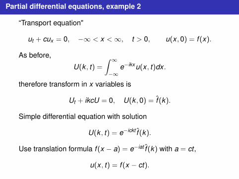
“Transport equation"
ut + cux = 0, −∞ < x <∞, t > 0, u(x ,0) = f (x).
As before,
U(k , t) =∫ ∞−∞
e−ikxu(x , t)dx .
therefore transform in x variables is
Ut + ikcU = 0, U(k ,0) = f (k).
Simple differential equation with solution
U(k , t) = e−ickt f (k).
Use translation formula f (x − a) = e−iat f (k) with a = ct ,
u(x , t) = f (x − ct).

Partial differential equations, example 2
“Transport equation"
ut + cux = 0, −∞ < x <∞, t > 0, u(x ,0) = f (x).
As before,
U(k , t) =∫ ∞−∞
e−ikxu(x , t)dx .
therefore transform in x variables is
Ut + ikcU = 0, U(k ,0) = f (k).
Simple differential equation with solution
U(k , t) = e−ickt f (k).
Use translation formula f (x − a) = e−iat f (k) with a = ct ,
u(x , t) = f (x − ct).
Partial differential equations, example 3
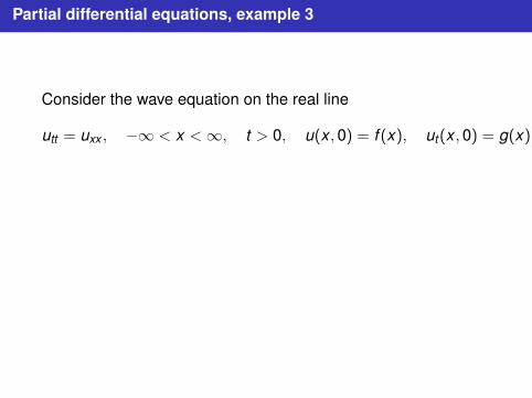
Consider the wave equation on the real line
utt = uxx , −∞ < x <∞, t > 0, u(x ,0) = f (x), ut(x ,0) = g(x).
Transforming as before,
Utt + k2U = 0, U(k ,0) = f (k), Ut(k ,0) = g(k).
Solution of initial value problem
U(k , t) = f (k) cos(kt) +g(k)
ksin(kt).

Partial differential equations, example 3
Consider the wave equation on the real line
utt = uxx , −∞ < x <∞, t > 0, u(x ,0) = f (x), ut(x ,0) = g(x).
Transforming as before,
Utt + k2U = 0, U(k ,0) = f (k), Ut(k ,0) = g(k).
Solution of initial value problem
U(k , t) = f (k) cos(kt) +g(k)
ksin(kt).

Partial differential equations, example 3
Consider the wave equation on the real line
utt = uxx , −∞ < x <∞, t > 0, u(x ,0) = f (x), ut(x ,0) = g(x).
Transforming as before,
Utt + k2U = 0, U(k ,0) = f (k), Ut(k ,0) = g(k).
Solution of initial value problem
U(k , t) = f (k) cos(kt) +g(k)
ksin(kt).
Partial differential equations, example 3, cont.
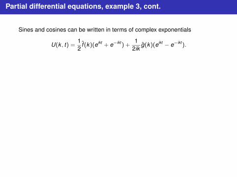
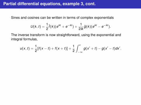
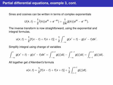
Sines and cosines can be written in terms of complex exponentials
U(k , t) =12
f (k)(eikt + e−ikt) +1
2ikg(k)(eikt − e−ikt).
The inverse transform is now straightforward, using the exponential andintegral formulas,
u(x , t) =12[f (x − t) + f (x + t)] +
12
∫ x
−∞g(x ′ + t)− g(x ′ − t)dx ′.
Simplify integral using change of variables∫ x
−∞g(x ′ + t)− g(x ′ − t)dx ′ =
∫ x+t
−∞g(ξ)dξ −
∫ x−t
−∞g(ξ)dξ =
∫ x+t
x−tg(ξ)dξ.
All together get d’Alembert’s formula
u(x , t) =12[f (x − t) + f (x + t)] +
12
∫ x+t
x−tg(ξ)dξ.
Partial differential equations, example 3, cont.
Sines and cosines can be written in terms of complex exponentials
U(k , t) =12
f (k)(eikt + e−ikt) +1
2ikg(k)(eikt − e−ikt).
The inverse transform is now straightforward, using the exponential andintegral formulas,
u(x , t) =12[f (x − t) + f (x + t)] +
12
∫ x
−∞g(x ′ + t)− g(x ′ − t)dx ′.
Simplify integral using change of variables∫ x
−∞g(x ′ + t)− g(x ′ − t)dx ′ =
∫ x+t
−∞g(ξ)dξ −
∫ x−t
−∞g(ξ)dξ =
∫ x+t
x−tg(ξ)dξ.
All together get d’Alembert’s formula
u(x , t) =12[f (x − t) + f (x + t)] +
12
∫ x+t
x−tg(ξ)dξ.

Fundamental solutions
Consider generic, linear, time-dependent equation
ut(x , t) = Lu(x , t), −∞ < x <∞, u(x ,0) = f (x), lim|x |→∞
u(x , t) = 0,
where L is some operator(e.g. L = ∂2/∂x2).
The fundamental solution S(x , x0, t) is a type of Green’sfunction, solving
St = LxS, −∞ < x <∞, S(x , x0,0) = δ(x−x0), lim|x |→∞
S(x , x0, t) = 0.
Initial condition means S limits to a δ-function as t → 0:
limt→0
∫ ∞−∞
S(x , x0, t)φ(x)dx =
∫ ∞−∞
δ(x − x0)φ(x)dx = φ(x0),

Fundamental solutions, cont.
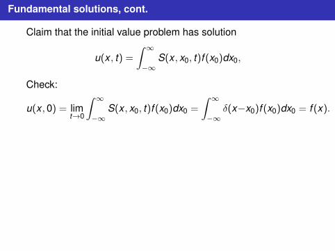
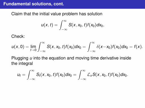
Claim that the initial value problem has solution
u(x , t) =∫ ∞−∞
S(x , x0, t)f (x0)dx0,
Check:
u(x ,0) = limt→0
∫ ∞−∞
S(x , x0, t)f (x0)dx0 =
∫ ∞−∞
δ(x−x0)f (x0)dx0 = f (x).
Plugging u into the equation and moving time derivative insidethe integral
ut =
∫ ∞−∞
St(x , x0, t)f (x0)dx0 =
∫ ∞−∞LxS(x , x0, t)f (x0)dx0.
Now move operator outside integral
ut = Lx
∫ ∞−∞
S(x , x0, t)f (x0)dx0 = Lxu.
Fundamental solutions, cont.
Claim that the initial value problem has solution
u(x , t) =∫ ∞−∞
S(x , x0, t)f (x0)dx0,
Check:
u(x ,0) = limt→0
∫ ∞−∞
S(x , x0, t)f (x0)dx0 =
∫ ∞−∞
δ(x−x0)f (x0)dx0 = f (x).
Plugging u into the equation and moving time derivative insidethe integral
ut =
∫ ∞−∞
St(x , x0, t)f (x0)dx0 =
∫ ∞−∞LxS(x , x0, t)f (x0)dx0.
Now move operator outside integral
ut = Lx
∫ ∞−∞
S(x , x0, t)f (x0)dx0 = Lxu.

Fundamental solutions using the Fourier transform, example 1
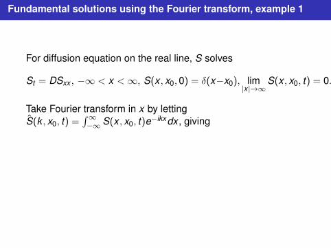
For diffusion equation on the real line, S solves
St = DSxx , −∞ < x <∞, S(x , x0,0) = δ(x−x0), lim|x |→∞
S(x , x0, t) = 0.
Take Fourier transform in x by lettingS(k , x0, t) =
∫∞−∞ S(x , x0, t)e−ikxdx , giving
St = −Dk2S, S(k ,0) = e−ix0k .
Solution to this ODE
S = e−ix0k−Dk2t .
Fundamental solutions using the Fourier transform, example 1
For diffusion equation on the real line, S solves
St = DSxx , −∞ < x <∞, S(x , x0,0) = δ(x−x0), lim|x |→∞
S(x , x0, t) = 0.
Take Fourier transform in x by lettingS(k , x0, t) =
∫∞−∞ S(x , x0, t)e−ikxdx , giving
St = −Dk2S, S(k ,0) = e−ix0k .
Solution to this ODE
S = e−ix0k−Dk2t .
Fundamental solutions using the Fourier transform, example 1
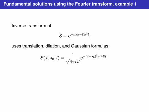
Inverse transform of
S = e−ix0k−Dk2t .
uses translation, dilation, and Gaussian formulas:
S(x , x0, t) =1√
4πDte−(x−x0)
2/(4Dt).
It follows that the solution to ut = Duxx and u(x ,0) = f (x) is
u(x , t) =∫ ∞−∞
f (x0)√4πDt
e−(x−x0)2/(4Dt)dx0.

Fundamental solutions using the Fourier transform, example 1
Inverse transform of
S = e−ix0k−Dk2t .
uses translation, dilation, and Gaussian formulas:
S(x , x0, t) =1√
4πDte−(x−x0)
2/(4Dt).
It follows that the solution to ut = Duxx and u(x ,0) = f (x) is
u(x , t) =∫ ∞−∞
f (x0)√4πDt
e−(x−x0)2/(4Dt)dx0.

Fundamental solutions using the Fourier transform, example 2
Linearized Korteweg - de Vries (KdV) equation:
ut = −uxxx , u(x ,0) = f (x), lim|x|→∞
u(x , t) = 0.
Fundamental solution solves
St = −Sxxx , S(x , x0,0) = δ(x − x0), lim|x|→∞
S(x , x0, t) = 0.
TransformingSt = ik3S, S(k ,0) = e−ix0k ,
whose solution is S(k , x0, t) = e−ix0k eik3t .Recall transform of Airy function Ai(x) is eik3/3, therefore
S(x , x0, t) =[e−ix0k eik3t
]∨=[ei(k/a)3/3
]∨(x − x0)
= aAi(
a(x − x0)), a ≡ (3t)−1/3.
Solution to original equation:
u(x , t) =1
(3t)1/3
∫ ∞−∞
Ai(
x − x0
(3t)1/3
)f (x0)dx0.

Fundamental solutions using the Fourier transform, example 2
Linearized Korteweg - de Vries (KdV) equation:
ut = −uxxx , u(x ,0) = f (x), lim|x|→∞
u(x , t) = 0.
Fundamental solution solves
St = −Sxxx , S(x , x0,0) = δ(x − x0), lim|x|→∞
S(x , x0, t) = 0.
TransformingSt = ik3S, S(k ,0) = e−ix0k ,
whose solution is S(k , x0, t) = e−ix0k eik3t .
Recall transform of Airy function Ai(x) is eik3/3, therefore
S(x , x0, t) =[e−ix0k eik3t
]∨=[ei(k/a)3/3
]∨(x − x0)
= aAi(
a(x − x0)), a ≡ (3t)−1/3.
Solution to original equation:
u(x , t) =1
(3t)1/3
∫ ∞−∞
Ai(
x − x0
(3t)1/3
)f (x0)dx0.

Fundamental solutions using the Fourier transform, example 2
Linearized Korteweg - de Vries (KdV) equation:
ut = −uxxx , u(x ,0) = f (x), lim|x|→∞
u(x , t) = 0.
Fundamental solution solves
St = −Sxxx , S(x , x0,0) = δ(x − x0), lim|x|→∞
S(x , x0, t) = 0.
TransformingSt = ik3S, S(k ,0) = e−ix0k ,
whose solution is S(k , x0, t) = e−ix0k eik3t .Recall transform of Airy function Ai(x) is eik3/3, therefore
S(x , x0, t) =[e−ix0k eik3t
]∨=[ei(k/a)3/3
]∨(x − x0)
= aAi(
a(x − x0)), a ≡ (3t)−1/3.
Solution to original equation:
u(x , t) =1
(3t)1/3
∫ ∞−∞
Ai(
x − x0
(3t)1/3
)f (x0)dx0.

Fundamental solutions using the Fourier transform, example 2
Linearized Korteweg - de Vries (KdV) equation:
ut = −uxxx , u(x ,0) = f (x), lim|x|→∞
u(x , t) = 0.
Fundamental solution solves
St = −Sxxx , S(x , x0,0) = δ(x − x0), lim|x|→∞
S(x , x0, t) = 0.
TransformingSt = ik3S, S(k ,0) = e−ix0k ,
whose solution is S(k , x0, t) = e−ix0k eik3t .Recall transform of Airy function Ai(x) is eik3/3, therefore
S(x , x0, t) =[e−ix0k eik3t
]∨=[ei(k/a)3/3
]∨(x − x0)
= aAi(
a(x − x0)), a ≡ (3t)−1/3.
Solution to original equation:
u(x , t) =1
(3t)1/3
∫ ∞−∞
Ai(
x − x0
(3t)1/3
)f (x0)dx0.

The method of images for fundamental solutions
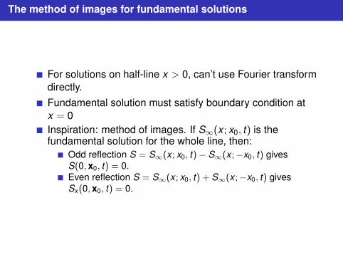
For solutions on half-line x > 0, can’t use Fourier transformdirectly.
Fundamental solution must satisfy boundary condition atx = 0Inspiration: method of images. If S∞(x ; x0, t) is thefundamental solution for the whole line, then:
Odd reflection S = S∞(x ; x0, t)− S∞(x ;−x0, t) givesS(0,x0, t) = 0.Even reflection S = S∞(x ; x0, t) + S∞(x ;−x0, t) givesSx(0,x0, t) = 0.

The method of images for fundamental solutions
For solutions on half-line x > 0, can’t use Fourier transformdirectly.Fundamental solution must satisfy boundary condition atx = 0
Inspiration: method of images. If S∞(x ; x0, t) is thefundamental solution for the whole line, then:
Odd reflection S = S∞(x ; x0, t)− S∞(x ;−x0, t) givesS(0,x0, t) = 0.Even reflection S = S∞(x ; x0, t) + S∞(x ;−x0, t) givesSx(0,x0, t) = 0.
The method of images for fundamental solutions
For solutions on half-line x > 0, can’t use Fourier transformdirectly.Fundamental solution must satisfy boundary condition atx = 0Inspiration: method of images. If S∞(x ; x0, t) is thefundamental solution for the whole line, then:
Odd reflection S = S∞(x ; x0, t)− S∞(x ;−x0, t) givesS(0,x0, t) = 0.Even reflection S = S∞(x ; x0, t) + S∞(x ;−x0, t) givesSx(0,x0, t) = 0.

The method of images for fundamental solutions, example
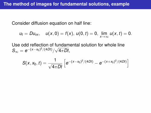
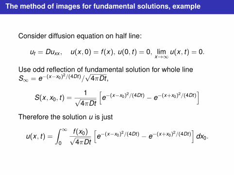
Consider diffusion equation on half line:
ut = Duxx , u(x ,0) = f (x), u(0, t) = 0, limx→∞
u(x , t) = 0.
Use odd reflection of fundamental solution for whole lineS∞ = e−(x−x0)
2/(4Dt)/√
4πDt ,
S(x , x0, t) =1√
4πDt
[e−(x−x0)
2/(4Dt) − e−(x+x0)2/(4Dt)
]Therefore the solution u is just
u(x , t) =∫ ∞
0
f (x0)√4πDt
[e−(x−x0)
2/(4Dt) − e−(x+x0)2/(4Dt)
]dx0.
The method of images for fundamental solutions, example
Consider diffusion equation on half line:
ut = Duxx , u(x ,0) = f (x), u(0, t) = 0, limx→∞
u(x , t) = 0.
Use odd reflection of fundamental solution for whole lineS∞ = e−(x−x0)
2/(4Dt)/√
4πDt ,
S(x , x0, t) =1√
4πDt
[e−(x−x0)
2/(4Dt) − e−(x+x0)2/(4Dt)
]
Therefore the solution u is just
u(x , t) =∫ ∞
0
f (x0)√4πDt
[e−(x−x0)
2/(4Dt) − e−(x+x0)2/(4Dt)
]dx0.
The method of images for fundamental solutions, example
Consider diffusion equation on half line:
ut = Duxx , u(x ,0) = f (x), u(0, t) = 0, limx→∞
u(x , t) = 0.
Use odd reflection of fundamental solution for whole lineS∞ = e−(x−x0)
2/(4Dt)/√
4πDt ,
S(x , x0, t) =1√
4πDt
[e−(x−x0)
2/(4Dt) − e−(x+x0)2/(4Dt)
]Therefore the solution u is just
u(x , t) =∫ ∞
0
f (x0)√4πDt
[e−(x−x0)
2/(4Dt) − e−(x+x0)2/(4Dt)
]dx0.
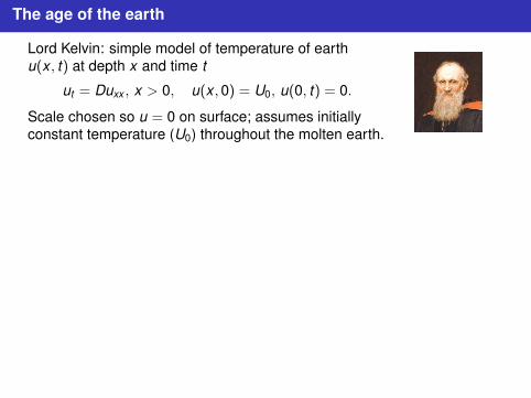
The age of the earth
Lord Kelvin: simple model of temperature of earthu(x , t) at depth x and time t
ut = Duxx , x > 0, u(x ,0) = U0, u(0, t) = 0.
Scale chosen so u = 0 on surface; assumes initiallyconstant temperature (U0) throughout the molten earth.
We found solution
u(x , t) =∫ ∞
0
U0√4πDt
[e−(x−x0)
2/(4Dt) − e−(x+x0)2/(4Dt)
]dx0.
Temperature gradient µ at surface is therefore
µ = ux(0, t) =U0√4πDt
1Dt
∫ ∞0
x0e−x20/(4Dt)dx0 =
U0√πDt
.
This relates the age of earth t to quantities we can estimate
U0 ≈ melting temp. of iron ≈ 104C, D ≈ 10−3m2/s, µ ≈ 10−2C/m,
which gives t ≈ 3× 10⁷ years !!??
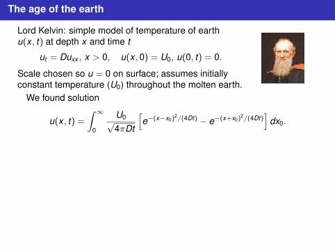