SOLUTIONS MANUAL -...

Soil Mechanics: concepts and applications 2nd edition SOLUTIONS MANUAL William Powrie

This solutions manual is made available free of charge. Details of the accompanying textbook Soil Mechanics: concepts and applications 2nd edition are on the website of the publisher www.sponpress.com and can be ordered from [email protected] or phone: +44 (0) 1264 343071 First published 2004 by Spon Press, an imprint of Taylor & Francis, 2 Park Square, Milton Park, Abingdon, Oxon OX14 4RN Simultaneously published in the USA and Canada by Spon Press 270 Madison Avenue, New York, NY 10016, USA @ 2004 William Powrie All rights reserved. No part of this book may be reprinted or reproduced or utilized in any form or by any electronic, mechanical, or other means, now known or hereafter invented, including photocopying and recording, or in any information storage or retrieval system, except for the downloading and printing of a single copy from the website of the publisher, without permission in writing from the publishers. Publisher's note This book has been produced from camera ready copy provided by the author with the assistance of Dr Joel Smethurst, University of Southampton, UK Contents Chapter 1 ..................................... 2 See separate file Chapter 2 ................................... 15 See separate file Chapter 3 ................................... 29 See separate file Chapter 4 ................................... 46 See separate file Chapter 5 ................................... 61 See separate file Chapter 6 ................................... 84 Chapter 7 ................................. 102 Chapter 8 ................................. 125 Chapter 9 ................................. 137 Chapter 10 ............................... 152 Chapter 11 ............................... 171

QUESTIONS AND SOLUTIONS: CHAPTER 6 Note: Questions 6.2 to 6.4 may be answered using either the Newmark chart (main text Figure 6.8), or Fadum's chart (main text Figure 6.14), or both. Question 6.5 is based on case study C6.1, and should therefore be answered with the aid of a Newmark chart. In these solutions, the Newmark chart method is used in all cases. Determining elastic parameters from laboratory test data Q6.1 (a) Write down Hooke's Law in incremental form in three dimensions and show that for undrained deformations Poisson's ratio νu = 0.5. Assuming that the behaviour of soil can be described in terms of conventional elastic parameters, show that in undrained plane compression (i.e. Δε2 = 0), the undrained Young's modulus E u is given by 0.75 × the slope of a graph of deviator stress q (defined as σ1-σ3) against axial strain ε1. Show also that the maximum shear strain is equal to twice the axial strain, and that the shear modulus G = 0.25 × (q/ε1). (b) Figure 6.20 shows graphs of deviator stress q and pore water pressure u against axial strain ε1 for an undrained plane compression test carried out at a constant cell pressure of 122 kPa. Comment on these curves and explain the relationship between them. Calculate and contrast the shear and Young's moduli at 1% shear strain and at 10% shear strain. Which would be the more suitable for use in design, and why? [University of London 2nd year BEng (Civil Engineering) examination, King's College (part question)] Q6.1 Solution (a) Writing Hooke's law for an isotropic, elastic material in terms of undrained parameters Eu and νu, and changes in principal total stress Δσ and changes in principal strain Δε, Δε1 = (1/Eu).(Δσ1-νuΔσ2-νuΔσ3) Δε2 = (1/Eu).(Δσ2-νuΔσ1-νuΔσ3) Δε3 = (1/Eu).(Δσ3-νuΔσ1-νuΔσ2) (main text Equation 6.1) __________________________ Δεvol = Δε1 + Δε2 + Δε3 = (1/Eu).(Δσ1 + Δσ2 + Δσ3).(1 - 2.νu) But in an undrained test Δεvol = 0, therefore (1 - 2.νu) = 0 ⇒ νu = 0.5 In a plane compression test, σ1 is increased while σ3 is kept constant, i.e. Δσ3 = 0. Also, the condition of plane strain ⇒ Δε2 = 0. Hence Δε2= (1/Eu).(Δσ 2 - Δσ1/2) = 0

⇒ Δσ 2 = Δσ1/2 (a) and Δε1 = (1/Eu).(Δσ1 - Δσ2/2) (b)

84

Substituting (a) into (b), Δε1 = (1/Eu).(Δσ1 - Δσ1/4) = 3Δσ1/4Eu or Δσ1/Δε1 = 4Eu/3 With Δσ3 = 0 (σ3 = constant), Δσ1 = Δ(σ1 – σ3) and Δε1 = ε1 so that Eu = 0.75 × Δ(σ1 – σ3)/Δε1 which is 0.75 times the slope of a graph of devator stress (σ1 – σ3) against axial strain ε1. εvol = ε1 + ε2 + ε3 = 0 and since ε2 = 0, ε1 + ε3 = 0 or ε3 = -ε1 From the Mohr circle of strain, γmax/2 = ε1 ⇒ γmax = 2ε1 From the Mohr circle of stress, τmax = (σ1 – σ3)/2 Hence the shear modulus G = τ/γ = (σ1 – σ3)/4ε1 = 0.25.q/ε1 where q is the deviator stress (σ1 – σ3) (b) The deviator stress rises with (axial) strain to a peak of about 112 kPa at an axial strain of about 3.4%. The deviator stress then falls quite rapidly to as possibly bsteady value (although the test has not been continued to a high enough strain to be sure of this) of about 87 kPa. It is likely that the sudden fall in deviator stress between 3.4% and 5% is due to the formation of a rupture. The pore water pressure rises with the deviator stress until an axial strain of about 0.8%, at which point the rate of change of pore pressure with deviator stress du/dq falls abruptly: this might indicate yield. The pore water pressure reaches a maximum of about 58 kPa at an axial strain of about 2.5%, and then starts to fall just before the peak deviator stress is reached. Again, it is possiblebut not certain that steady conditions have been reached by the end of the test at an axial strain of 5%. Using the relationships determined in part (a) and scaling values of deviator stress from the stress-strain curve at the appropriate strains,

i) at γ = 1%, ε1 = γ/2 = 0.5% and (from the graph) q = (σ1 – σ3) ~ 67.5 kPa; hence using G = 0.25.q/ε1 Gγ=1% = 67.5 kPa ÷ (4 × 0.005) = 3375 kPa

ii) at γ = 10%, ε1 = γ/2 = 5% and (from the graph) q = (σ1 – σ3) ~ 87 kPa; hence using G = 0.25.q/ε1 Gγ=1% = 87kPa ÷ (4 × 0.05) = 435 kPa

85

The shear modulus at γ = 10% is a factor of almost ten smaller than at γ = 1%: the tangent shear modulus at γ = 10% may even be negative! The shear modulus at γ = 1% is the more suitable for use in design, as shear strains of 10% would be unacceptably large in practice (in fact, a shear strain of even 1% is quite large for a foundation or a retaining wall). Calculation of increases in vertical effective stress below a surface surcharge Q6.2 The foundation of a new building may be represented by a raft of plan dimensions 10 m × 6 m, which exerts a uniform vertical stress of 50kPa at founding level. A pipeline AA' runs along the edge of the building at a depth of 2m below founding level, as indicated in plan view in Figure 6.21. Estimate the increase in vertical stress at a number of points along the pipeline AA', due to the construction of the new building. Present your results as a graph of increase in vertical stress against distance along the pipeline AA', indicating the extent of the foundation on the graph. What is the main potential shortcoming of your analysis? [University of London 2nd year BEng (Civil Engineering) examination, Queen Mary and Westfield College] Q6.2 Solution Set the “scale for Z” = 2 m and draw plan views of the foundation to this scale, with the points where the increase in σv is to be calculated located above the centre of the chart. The locations of points A to H are as indicated in the sketch below, and the Newmark chart with the foundation positions indicated in each case is given in Figure Q6.2a.

86

Figure Q6.2a: Newmark chart for Q6.2 The increase in vertical total stress Δσv below each of the points A to H is given by Δσv = (n/200) × 50 kPa where n is the number of elements on the chart covered by the foundation, as determined from the Newmark chart.

Point A B C D E F G H Distance from centreline, m 0 1 3 4 5 6 7 9

87

Number of elements covered, n 98 97 91 77.5 50 22.5 9 3 Δσv, kPa 24.5 24.3 22.8 19.4 12.5 5.6 2.3 0.8 The tabulated data are used to plot a graph of increase in vertical stress against distance along the pipeline in Figure Q6.2b (note the graph is symmetrical about the centreline; only one half is shown).

Figure Q6.2b: Increase in vertical stress against distance along the pipeline The main potential shortcoming of the analysis is that the pipe may act as a stiff inclusion, attracting more load than indicated by the elastic stress distribution on which the Newmark chart is based. Calculation of increases in vertical effective stress and resulting soil settlements Q6.3 (a) In what circumstances might an elastic analysis be used to calculate the changes in stress within the body of the soil due to the application of a surface surcharge? (b) Figure 6.22 shows a cross-section through a long causeway. Using the Newmark chart or otherwise, sketch the long-term settlement profile along a line perpendicular to the causeway. Given time, how might your analysis be refined? [University of London 2nd year BEng (Civil Engineering) examination, King's College] Q6.3 Solution (a) An elastic analysis might reasonably be used for small changes in stress and strain. Also, the soil muct be overconsolidated (ie on an unload/reload line) for its behaviour to be approximately reversible – otherwise, the loading must all be in the same direction (either loading or unloading).

88

(b) Refer to the Newmark Charts in Figures Q6.3b, c and d: note the extensive use of symmetry to avoid repetitive calculations. The causeway exerts a surcharge of 5 m × 20 kN/m3 = 100 kPa on the original soil surface, which may reasonably be treated as flexible. We know that for a strip footing, the increase in vetical stress below the centreline has fallen to 90% of that at the surface at a depth of about six times the footing width (see main text page section 6.3 and Figure 6.7) – in this case about 30 m. Divide the soil into three layers, 5 m, 10 m and 20 m thick. Calculate the increase in vertical effective stress Δσ'v at the mid-point of each layer, i.e. at depths of 2.5 m, 10 m and 25 m, and take these as the representative increases in vertical stress for each layer. The average one-dimensional stiffness of each layer is that at the centre, i.e. E'0 = (2000 + 1000z) kPa with z = 2.5 m, 10 m and 25 m giving E'0 = 4500 kPa, 12000 kPa and 27000 kPa respectively. To obtain a profile of settlement along a line perpendicular to the causeway, we will need to calculate the increases in vertical effective stress at each of these depths at points on the centreline of the causeway (point O on plan), halfway between the middle and the edge of the causeway (point E), the edge of the causeway (point A), and at distances of 2.5 m (point F), 5 m (point B), 10 m (point C) and 20 m (point D) from the edge (Figure Q6.3a).

B AFD C E O

2.5 m

2.5 m2.5 m

5 m10 m

Edge of the causeway

Figure Q6.3a: location of settlement calculation points relative to the centreline of the causeway In each of the Newmark charts that follow, the causeway is drawn with the “scale for Z” set to (i) 2.5 m (Figure Q6.3b), (ii) 10 m (Figure Q6.3c) and (iii) 25 m (Figure Q6.3c), such that the point at which it is sought to calculate the increase in vertical effective stress (O, A, B etc) is located above the centre of the chart. The increase in stress is then given by Δσv = (n/200) × 100 kPa, where n is the number of elements covered by the plan view of the causeway for the whole chart. Where symmetry is used and only a half or a quarter of the causeway is drawn, n is the number of elements counted multiplied by two or four respectively. The compression or settlement ρ of each soil layer of thickness t is calculated from the representative increase in vertical effective stress within the layer, ρ = Δσ'v.t/ E'0. (i) Figure Q6.3b, scale for Z set to 2.5 m, E'0 = 4500 kPa, layer thickness t = 5 m

89

Point O E A F B C D Number of elements covered, n 41 × 4 74 × 2 47½ × 2 9 × 2 2 × 2 ~ 0 ~ 0Δσ'v, kPa = (n/200) × 100 kPa 82 72 47.5 9 2 0 0 settlement ρ = Δσ'v.t/ E'0 91.1 82.2 52.8 10 2.2 0 0 (ii) Figure Q6.3c, scale for Z set to 10 m, E'0 = 12000 kPa, layer thickness t = 10 m Point O E A F B C D Number of elements covered, n

16½ × 4

29½ × 2

28 × 2

20 × 2

13 × 2

4½ × 2

1 × 2

Δσ'v, kPa = (n/200) × 100 kPa

33 29.5 28 20 13 4.5 1

settlement ρ = Δσ'v.t/ E'0 27.5 24.6 23.3 16.7 10.8 3.8 0.8 (iii) Figure Q6.3d, scale for Z set to 25 m, E'0 = 27000 kPa, layer thickness t = 20 m Point O E A F B C D

Number of elements covered, n 6¾ × 4 12½ × 2 12½ × 2 11½ × 2 10½ × 2 8 × 2 3½ × 2

Δσ'v, kPa = (n/200) × 100 kPa 13.5 12.5 12.5 11.5 10.5 8 3.5

settlement ρ = Δσ'v.t/ E'0 10.0 9.3 9.3 8.5 7.8 5.9 2.6

Summing the settlements, we have Point O E A F B C D Dist from centreline, m 0 1.25 2.5 5.0 7.5 12.5 22.5Total settlement, mm 130 116 85 35 21 10 3 The settlement profile is plotted in Figure Q6.3e

90

Figure Q6.3b: Newmark chart for x = 2.5 m

91

Figure Q6.3c: Newmark chart for x = 10 m

92

Figure Q6.3d: Newmark chart for x = 25 m

93

Figure Q6.3e: surface settlement profile The analysis could be refined by dividing the soil into more layers. Q6.4 (a) When might an elastic analysis reasonably be used to calculate the settlement of a foundation? Briefly outline the main difficulties encountered in converting stresses into strains and settlements. (b) A square raft foundation of plan dimensions 5 m × 5 m is to carry a uniformly distributed load of 50 kPa. A site investigation indicates that the soil has a one-dimensional modulus given by E'o = (10 + 6z) MPa, where z is the depth below the ground surface in metres. Use a suitable approximate method to estimate the ultimate settlement of the raft. [University of London 2nd year BEng (Civil Engineering) examination, King's College] Q6.4 Solution (a) An elastic analysis might reasonably be used if the soil is overconsolidated (on an unloading/reloading line) and the changes in stress and strain are small. The main difficulty in attempting to convert an elastic stress distribution into strains (and settlements) is the choice of an appropriate elastic modulus that takes proper account of the stress paths followed by all the soil elements. The usual approach is to use the one-dimensional modulus on the assumption that deformations are predominantly vertical. A possible problem that then arises is that this approach can only be used to calculate long-term, drained settlements after any excess pore water pressures induced by loading have dissipated, although empirical adjustments are available to estimate the short term settlements due to shearing of the soil at constant volume. (b) The soil nearer the surface will have more influence on settlements, as the stresses are greater and the modulus is less. The solution procedure is as follows.

1. Divide the soil into three layers 2. Use the Newmark chart to calculate the increase in vertical effective stress at the

middle of each layer (assuming that the surcharge can be idealised as flexible) 3. Use the value of E'0 at the centre of the layer to calculate the compression of the layer

(assuming deformation is primarily due to one dimensional compression).

94

Recalling that the increase in vertical effective stress below the centreline falls to approximately 10% of its value at the surface at a depth of twice the footing diameter, choose layer thicknesses of 4 m (0 to 4 m below ground level – centre of layer at 2 m below ground level); 4 m (4 m to 8 m below ground level – centre of layer at 6 m below ground level); and 8 m (8 m to 16 m below ground level – centre of layer at 12 m below ground level). Figure Q6.4 (the Newmark chart) shows plan views of the foundation with the “scale for Z” set to (i) 2 m, (ii) 6 m and (iii) 12 m, located so that the centre (solid line, one quarter of the foundation shown so that the actual number of elements covered has to be multiplied by four), a corner (chain dotted line, full foundation shown), and the middle of one side (dashed line, one half of the foundation shown so that the actual number of elements covered has to be multiplied by two) lie above the centre of the chart. The increase in stress in each case is calculated as Δσ'v = (n/200) × 50 kPa where n is the number of elements covered by the whole foundation. The compression of each layer is calculated as ρ = t. Δσ'v /E'0, where t is the thickness of the layer and E'0 = (10 + 6z) MPa giving E'0 = 22 MPa at z = 2 m, 46 MPa at z = 6 m, and 82 MPa at z = 12 m. The numbers of chart elements covered and the increases in vertical effective stress at each depth, and the layer and total settlements, are given in the Table below. Scale for Z, m

Location on foundation

Number of chart elements covered, n

Increase in vertical effective stress, Δσ'v = (n/200) × 50 kPa

Layer compression ρ = t. Δσ'v/E'0, mm

2 Centre 158 39.5 7.2 6 Centre 50 12.5 1.1 12 Centre 16 4 0.4 TOTAL 8.7 2 Corner 48 12 2.2 6 Corner 30 7.5 0.7 12 Corner 12 3 0.3 TOTAL 3.2 2 Mid-side 86 21.5 3.9 6 Mid-side 38 9.5 0.8 12 Mid-side 14 3.5 0.3 TOTAL 5.0

95

Figure Q6.4. Newmark chart for Q6.4 The total settlements below the centre, corners and mid-sides of 8.7 mm, 3.2 mm and 5.0 mm respectively would be for a prefectly flexible footing. For a rigid footing where the loading on the fooring was 50 kPa, we might estimate the average settlement as ρrigid ≈ [(4 × 5.0 mm) + (4 × 3.2 mm) + ( 1 × 8.7 mm)] ÷ 9 = 4.6 mm

96

Q6.5 The foundations of a new building may be represented by a raft of plan dimensions 24 m × 32 m, which exerts a uniform vertical stress of 53.5kPa at founding level. The soil at the site comprises laminated silty clay underlain by firm rock. The estimated stiffness in one-dimensional compression E'o increases with depth as indicated below. Depth below founding level, m

E'o, MPa

0 to 4 5 4 to 10 10 10 to 20 25 below 20 very stiff Use the Newmark chart (Figure 6.8) to estimate the increase in vertical stress at depths of 4 m, 10 m and 20 m below the centre of the raft. Hence estimate the expected eventual settlement of the centre of the foundation. Suggest two possible shortcomings of your analysis. [University of London 2nd year BEng (Civil Engineering) examination, Queen Mary and Westfield College] Q6.5 Solution To calculate the increases in vertical effective stress at depths of 4 m, 10 m and 20 m, set the “scale for Z” on the Newmark chart to each of these values in turn. Draw plan views of the foundation, to these scales, with the centre of the foundation above the centre of the chart (see Figure Q6.5, and note that with Z = 4 m the foundation covers the entire chart). Using symmetry, it is necessary only to draw one quarter of the foundation in each case. The increase in stress below the centre is given by Δσ'v = (n/200) × 53.5 kPa where n is the number of elements covered by the whole foundation. The compression of each layer is ρ = t. Δσ'v /E'0, where t is the thickness of the layer and E'0 is the one dimensional modulus. Hence Depth, m 4 10 20 Number of elements covered, n 50 × 4 40¾ × 4 24 × 4 Increase in vertical effective stress Δσ'v = (n/200) × 53.5 kPa

53.5 43.6 25.7

97

Figure Q6.5. Newmark chart Layer depth, m below ground level

Average increase in vertical effective stress Δσ'v,average, kPa

Layer thickness t, m

E'0, MPa

Layer compression ρ, mm

0 – 4 53.5 4 5 42.8 4 – 10 48.6 6 10 29.2 10 – 20 34.7 10 25 13.9 below 20 not calculated - ∞ 0 TOTAL 86

98

The total settlement is therefore 86 mm The main shortcomings of the analysis are

1. The raft foundation is stiff, so the loading transmitted to the soil will not in fact be uniform

2. The division of the soil into only three layers is quite crude and could be refined 3. It has been assumed that deformation is essentially by one dimensional compression,

i.e. shear deformation at constant volume has been neglected 4. The use of the elastic soil model may be unrealistic

(two only required). Use of standard formulae in conjunction with one-dimensional consolidation theory (Chapter 4) Q6.6 (a) To estimate the ultimate settlement of the grain silo described in Q4.5, the engineer decides to assume that the soil behaviour is elastic, with the same properties in loading and unloading. In what circumstances might this be justified? (b) The proposed silo will be founded on a rigid circular foundation of diameter 10 m. Under normal conditions, the net or additional load imposed on the soil by the foundation, the silo and its contents will be 5 000 kN. What is the ultimate settlement due to this load? (It may be assumed that the settlement ρ of a rigid circular footing of diameter B carrying a vertical load Q at the surface of an elastic half space of one-dimensional modulus E'o and Poisson's ratio ν'

is given by ρ = (Q/E'oB).[(1-ν')2/(1-2ν')]. Take ν' = 0.2) (c) To reduce the time taken for the settlement to reach its ultimate value, it is proposed to overload the foundation initially by 5000 kN, the additional load being removed when the settlement has reached 90% of the predicted ultimate value. In practice, this occurs after six months has elapsed, and the additional load is then removed. Giving two or three actual values, sketch a graph showing the settlement of the silo as a function of time. (Assume that the principle of superposition can be applied, and use the curve of R against T given in Figure 4.18.) State briefly the main shortcomings of your analysis. [University of London 2nd year BEng (Civil Engineering) examination, King's College (part question)] Q6.6 Solution (a) The assumption that the soil is elastic with the same properties in loading and unloading is justified if the soil is overconsolidated, i.e. it is on an “elastic” unload/reload line, and that the changes in stress and strain are small. (b) The ultimate settlement when all excess pore water pressures have dissipated is given by ρ = (Q/E'0B).[(1-ν')2 /(1-2ν')]

99

(Note: this Equation can be recovered by writing E' and ν' in place of E and ν in main text Equation 6.14 (page 352), and substituting main text Equation 6.10 (page 344), E' = E'0.[(1 + ν').(1 – 2ν')]/(1 - ν')). Substituting the values given of Q = 5 000 kN, B = 10 m, E'0 =10 000 kPa and ν' = 0.2, ρ (m) = [5 000 kN ÷ (10 000 kPa × 10 m)) × [(0.8)2 ÷ 0.6] ⇒ ρ = 53 mm (c) Assume that the settlement vs time relationship can be based approximately on the one-dimensional comsolidation of a clay layer of thickness d with one-way drainage, in response to an increase in vertical stress of Q/(πB2/4). The ultimate settlement with a load of 10 000 kN is 106 mm. The additional 5 000 kN load is removed when ρ = 0.9 × 53 mm, or at R = ρ/ρult for the load of 10 000 kN = 0.45. From the curve of R against T given in main text Figure 4.18, T = (cv.t/d2) ≈ 0.15 when R = 0.45. We can use the fact that T = 0.15 after six months to calculate the effective drainage path length (assuming one-way drainage to the surface), d: T = (cv.t/d2) = 0.15 when t = 6 months = 259 200 minutes, and cv = 2.12 mm2/minute from Q4.5. Thus d2 = cv.t/0.15 = 2.12 mm2/min × 259 200 min ÷ 0.15 ⇒ d2 = 3.66 × 106 mm2, or d ~ 1.91 m [note that within this depth, which corresponds to about 0.2 times the silo diameter of 10 m, the increase in vertical stress is approximately constant at below most of the foundation: see main text Figure 6.7] The analysis of the consolidation process given in main text Section 4.5 shows that the settlement ρ is proportional to √t until t = d2/12cv which is in this case 100 days (t = [3.66 × 106 mm2] ÷ [12 × 2.12 mm2/min] = 144 000 min = 100 days). After 6 months, when the overload of 5 000 kN is removed, superimpose the solutions for (A) loading of 10 000 kN at t = 0, and (B) unloading of 5 000 kN at t = 6 months, using values of T and R taken from main text Equations 4.22 and 4.23 or main text Figure 4.18. After 12 months

TA = 0.30 TB = 0.15 B

RA = 0.65RB = 0.45B

ρ = (0.65 × 106 mm) – (0.45 × 53 mm)

ρ = 45 mm

After 2 years TA = 0.60 TB = 0.45 B

RA = 0.86RB = 0.77B

ρ = (0.86 × 106 mm) – (0.77 × 53 mm)

ρ = 50 mm

After 3 years TA = 0.90 TB = 0.75 B

RA = 0.94RB = 0.91B

ρ = (0.94 × 106 mm) – (0.91 × 53 mm)

ρ = 51 mm

A graph of settlement against time is plotted in Figure Q6.6.

100

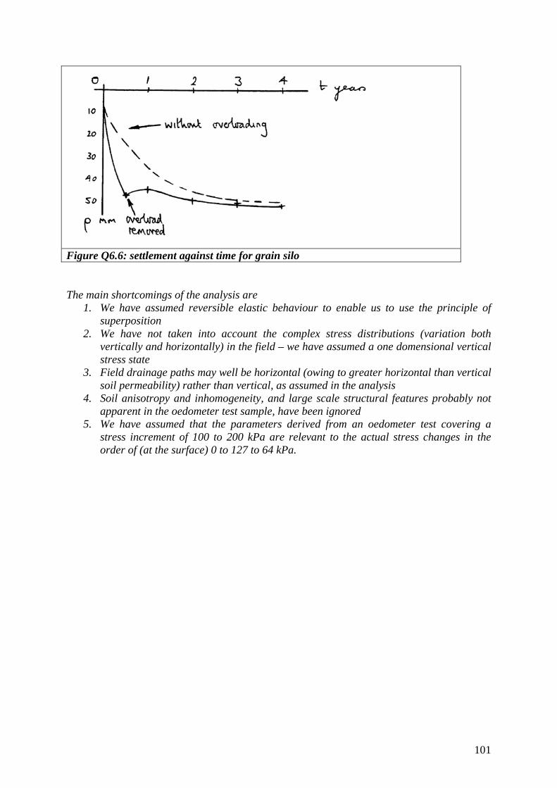
Figure Q6.6: settlement against time for grain silo The main shortcomings of the analysis are

1. We have assumed reversible elastic behaviour to enable us to use the principle of superposition

2. We have not taken into account the complex stress distributions (variation both vertically and horizontally) in the field – we have assumed a one domensional vertical stress state

3. Field drainage paths may well be horizontal (owing to greater horizontal than vertical soil permeability) rather than vertical, as assumed in the analysis

4. Soil anisotropy and inhomogeneity, and large scale structural features probably not apparent in the oedometer test sample, have been ignored

5. We have assumed that the parameters derived from an oedometer test covering a stress increment of 100 to 200 kPa are relevant to the actual stress changes in the order of (at the surface) 0 to 127 to 64 kPa.

101

QUESTIONS AND SOLUTIONS: CHAPTER 7 Calculation of lateral earth pressures and prop loads Q7.1 (a) Explain the terms "active" and "passive" in the context of a soil retaining wall. (b) Figure 7.47 shows a cross section through a trench support system, which is formed of a rigid reinforced concrete U-section. Assuming that the retained soil is in the active state, and that the interface friction between the soil and the wall is zero, calculate and sketch the short-term distributions of horizontal total and effective stress and pore water pressure acting on the vertical member AB. (c) Hence calculate the axial load (in kN per metre length of the trench) in the horizontal member BC, and the bending moment (in kNm/m) at B. (d) Would you expect the axial load in BC and the bending moment at B to increase or decrease in the long term, and why? [University of London 2nd year BEng (Civil Engineering) examination, Queen Mary and Westfield College] Q7.1 Solution (a) “Active”: soil is on the verge of failure with lateral support being removed. Lateral stress is as small as possible for a given vertical stress, e.g. behind a retaining wall. “Passive”: soil is on the verge of failure with lateral stress being increased. Lateral stress is as large as possible for a given vertical stress, e.g. in front of an embedded retaining wall. (b) Assuming fully active conditions, i.e. the minimum possible lateral stress, In the sandy gravel (in terms of effective stresses), σ'h = Ka.σ'v, where Ka = (1 -sinφ')/(1 + sinφ') and with φ' = 35º, Ka = 0.271 In the clay (undrained in terms of total stresses), σh = σv – 2.τu; τu = 30 kPa Hence Depth, m Stratum σv, kPa u, kPa σ'v, kPa σ'h, kPa σh, kPa0 sandy gravel 20 0 20 5.4 5.4 4 sandy gravel 100 40 60 16.3 56.3 4 clay 100 (40) - - 40 6 clay 134 (60) - - 74 The vertical total stress σv at each depth is calculated from the surcharge (20 kPa) plus the weight of the overlying soil. The vertical effective stress σ'v = σv – u. Pore pressures in brackets are those that would act in a flooded tension crack at the interface between the clay and the wall when filled with water to the level of the ground surface: provided the minimum (active) total lateral stress within the clay is greater than or equal to this value (as is the case here), a tension crack will not form. The resulting stress distribution is shown in Figure Q7.1.

102

Figure Q7.1: Lateral stresses acting on retaining wall member AB, Q7.1 (c) The condition of horizontal equilibrium is used to calculate the axial load in BC, FBC. Considering the total stresses, FBC = [½ × (5.4 + 56.3) × 4] + [½ × (40 + 74) × 2] ⇒ FBC = 237.4 kN/m Taking moments about B, the bending moment at B, MB, is B

MB = [5.4 × 4 × 4] + [½ × 50.9 × 4× 3.33] + [40 × 2 × 1] + [½ × 34 × 2× /B

23]

⇒ MB = 528 kNm/mB (d) The structural loads would be expected to increase in the long term. This is because the clay has been unloaded laterally and therefore probably has negative pore pressures within it. As the negative pore pressures dissipate, the total load from the clay will increase. To calculate the long term loads, an effective stress analysis should be used.

103

Stress field limit equilibrium analysis of an embedded retaining wall Q7.2 (a) Figure 7.48 shows a cross section through a smooth embedded retaining wall, propped at the crest. Show that the wall would be on the verge of failure if the strength (angle of friction) of the soil were 18°. (Take the unit weight of water γw=10kN/m3.) (b) Sketch the distributions of lateral stress on both sides of the wall, and calculate the bending moment at formation level and the prop force. (c) If in fact the critical state strength of the soil is 24°, calculate the mobilization factor M = tanφ'crit/tanφ'mob. [University of London 3rd year BEng (Civil Engineering) examination, Queen Mary and Westfield College (part question)] Q7.2 Solution (a, b) Assuming fully active conditions, i.e. the minimum possible lateral stress, with φ' = 18° and soil/wall friction δ = 0, Behind the wall, conditions are active with σ'h = Ka.σ'v, where Ka = (1 -sinφ')/(1 + sinφ') and with φ' = 18º, Ka = 0.528 In front of the wall, conditions are passive with σ'h = Kp.σ'v, where Kp = (1 + sinφ')/(1 - sinφ') = 1/Ka = 1.894 Hence the lateral stresses acting on the wall at key depths, between which the lateral stress varies linearly, are Behind wall Depth, m σv, kPa u, kPa σ'v, kPa σ'h, kPa0 (ground surface) 0 0 0 0 10 (water table) 200 0 200 105.6 25.2 (toe of wall) 504 152 352 185.86 In front of wall Depth, m σv, kPa u, kPa σ'v, kPa σ'h, kPa0 (ground surface) 0 0 0 0 15.2 (toe of wall) 304 152 152 287.89 The vertical total stress σv at each depth is calculated from the weight of the overlying soil (there is no surcharge in this case). The vertical effective stress σ'v = σv – u. The resulting stress distribution is shown in Figure Q7.2.

104

Figure Q7.2: Lateral stresses acting on retaining wall, Q7.2 Note that the pore water pressures are hydrostatic below the same groundwater level on both sides of the wall, and therefore cancel out. This is NOT a general result: this is a special case because the water table is at the level of the excavated soil surface on both sides of the wall. Check that the stress distribution shown in Figure Q7.2 is in moment equilibrium about the prop (horizontal equilibrium will be satisfied by the prop load): Moments clockwise, given in the format [average lateral stress × depth of stress block × lever arm about the prop] are [½ × 105.6 × 10× 6.67] + [105.6 × 15.2 × 17.6] + [½ × 80.26 × 15.2× 20.13] = 44052.7 kNm/m Moments anticlockwise are [½ × 287.89 × 15.2× 20.13] = 44043.7 kNm/m The error is 9/44000 = 0.02%, which is negligible so the condition of equilibrium is satisfied. The prop load P is calculated from the condition of horizontal force equilibrium, P = [½ × (185.86 + 105.6) × 15.2] + [½ × 105.6 × 10] - [½ × 287.89 × 10] ⇒ P = 555 kN/m (The pore pressures have been ignored because they are exactly the same on both sides of the wall. As already stated, this is NOT a general result and it will normally be necessary to take the pore water pressures, which will usually be different on each side of the wall, into account in the equilibrium calculation).

105

The bending moment at formation level is given by M = [10 × 555.132 kN/m] – [½× 105.6 kPa × 10 m × 10 m/3] = 3791 kNm/m (c) The strength mobilization factor or factor of safety on soil strength is given by M = tan24° ÷ tan18° = 1.37 Q7.3 (a) Figure 7.49 shows a cross section through a rough embedded retaining wall, propped at the crest. Stating any assumptions you make, estimate the long term pore water pressure distribution around the wall. (b) Assuming that the critical state angle of soil friction of 35° is fully mobilized in the retained soil, calculate the earth pressure coefficient (based on effective stresses) in the soil in front of the wall required for moment equilibrium about the prop. Using Table 7.7, estimate the corresponding mobilized friction angle in the soil in front of the wall. (c) Is the wall safe? Explain briefly your reasoning. (Take the unit weight of water γw=10kN/m3). [University of London 3rd year BEng (Civil Engineering) examination, Queen Mary and Westfield College] Q7.3 Solution (a) Calculate the long-term pore water pressures assuming steady state seepage using the linear seepage approximation (see main text section 7.8.1, p416). The fall in head from h = 0 at the excavated soil surface to h = 4.5 m at the groundwater level on the retained side of the wall is assumed to be linear around the wall, giving a head at the toe of htoe = (3 m ÷ 10.5 m) × 4.5 m = 1.286 m and a pore water pressure of utoe = γw × (3 m + htoe) = 42.86 kPa (Figure Q7.3a)

106

Figure Q7.3a: Pore water pressures according to the linear seepage approximation (b) Investigate the equilibrium of the wall, assuming that the full soi strength of 35° is mobilized in the retained soil. The wall is rough, the angle of soil/wall friction δ = φ' = 35°, which gives an active earth pressure coefficient Ka of 0.2117 according to Table 7.6. Let the mobilized earth pressure coefficient in front of the wall be Kp. The vertical and horizontal total and effective stresses and pore pressures at key depths behind and in front of the wall are calculated in the table below. Behind wall Depth, m σv, kPa u, kPa σ'v, kPa

(=σv – u) σ'h, kPa (= Ka × σ'v)

σh, kPa (=σ'h+ u)

0 (ground surface) 0 0 0 0 0 3.5 (water table) 70 0 70 14.82 14.82 11 (toe of wall) 220 42.86 177.14 37.51 80.37 In front of wall Depth, m σv, kPa u, kPa σ'v, kPa

(=σv – u) σ'h, kPa (= Kp × σ'v)

σh, kPa (=σ'h+ u)

0 (ground surface) 0 0 0 0 0 3 (toe of wall) 60 42.86 17.14 17.14 × Kp 17.14Kp + 42.86 The stress distribution is shown schematically in Figure Q7.3b.

107

Figure Q7.3b: Total lateral stresses

14.82 kPa

17.14.Kp + 80.37 kPa

Take moments about the position of the prop to calculate the value of Kp needed for equilibrium: The overturning moment is MOT = [½ × 14.82 × 3.5 × 3.5 × 2/3] + [14.82 × 7.5 × (3.5 + {7.5 × ½})] + [½ × (80.37 – 14.82) × 7.5 × (3.5 + {7.5 × 2/3})] = 2955.76 kNm/m The restoring moment is MRE = [½ × (17.14Kp + 42.86) × 3 × (8 + {3 × 2/3})] = (257.1Kp + 642.9) kNm/m Thus 257.1Kp =2312.9 or Kp ~ 9 By interpolation from main text Table 7.7 (p 424), this requires a mobilized effective angle of friction (assuming full wall friction, δ = φ' ) of just over 35.5°. (c) The wall will probably collapse, because the required mobilized strength in front of the wall is greater than the critical state strength of the soil. Q7.4 Figure 7.50 shows a cross-section through a long excavation whose sides are supported by propped cantilever retaining walls. Calculate the depth of embedment needed just to prevent undrained failure by rotation about the prop if the groundwater level behind the wall is (i) below formation level; and (ii) at original ground level. neglect the effects of friction/adhesion at the soil/wall interface, and take the unit weight of water as 10 kN/m3. What is the strut load in each case?

108

Q7.4 Solution In the gravel for a frictionless wall, Ka = (1 - sinφ')/ (1 - sinφ') = 0.271 with φ' = 35°. (i) With the water table below formation level, the pore water pressures in the gravel are zero and the lateral effective stress increases from zero at original ground level to Ka × σ'v = 0.271 × 20 kN/m3 × 2 m = 10.84 kPa at depth 2 m, the interface between the gravel and the clay. In the clay, a dry tension crack might extend to a depth z below origilal ground level such that σv = 2.τu, or 20z = 160 kPa ⇒ z = 8 m (below original ground level). Below this depth, the horizontal total stress behind the wall is given by σh = σactive = γ.z – 2τu = (160 + 20.x) – 160 = 20.x kPa where x is the depth in m below the bottom of the tension crack, ie x = (z – 8) where z is the depth below original ground level. Note that x is also the depth below formation level. In front of the wall, the horizontal total stress is given by σh = σpassive = γ.z + 2τu = 20.x + 160 kPa where x is the depth in m below formation level. The resulting stress distribution is shown in Figure Q7.4a: note that the triangular components of the total stress distribution on either side of the wall below formation level cancel out.

Figure Q7.4a: lateral total stresses on retaining wall with water table below formation level Take moments about the position of the prop to find the value of x required for (moment) equilibrium: (½ × 10.84 kPa × 2 m) × (2/3 × 2 m) = (160 kPa × x m) × (8 + ½x) m ⇒ 80x2 + 1280 x – 14.45 = 0, or x2 + 16 x – 0.180625 = 0

109

⇒ x = {-16 ± √(162 + [4 × 0.180625])} ÷ 2 ⇒ x = 0.01 m (0.01128) The prop force F is calculated from the condition of horizontal equilibrium, F = (10.84 – 160 x) = 9 kN/m Note that the critical mode of failure in this case would be base instability, and the depth of embedment would need to be increased to prevent this. (ii) With the water table at original ground level, the effect of the pore water pressures must be taken into account. Assume that the pore water pressures in the gravel are hydrostatic. The pore water pressure at 2 m depth is 2 m × 10 kN/m3 = 20 kPa, and the vertical total stress is 2 m × 22 kN/m3 = 44 kPa, so the vertical effective stress is 44 kPa – 20 kPa = 24 kPa. The lateral effective stress increases from zero at original ground level to Ka × σ'v = 0.271 × 24 kPa = 16.5 kPa at 2 m depth. The lateral total stress is equal to the lateral effective stress plus the pore water pressure, σh = σ'h + u = 26.5 kPa. In the clay, a flooded tension crack might extend to a depth z below original ground level such that (σv – σh) = 2.τu with σv = (20 z + 4) kPa and σh = γw.z = 10 z kPa. Hence 20 z + 4 – 10 z = 160 kPa ⇒ 10 z = 156 m, or z = 15.6 m (below original ground level). In front of the wall, the horizontal total stress is given (as before) by σh = σpassive = γ.z + 2τu = 20.x + 160 kPa where x is the depth in m below formation level. Assuming that the required depth of embedment x is not greater than 7.6 m (so that z ≤ 15.6 m), the resulting stress distribution is shown in Figure Q7.4b. Take moments about the position of the prop to find the new equilibrium value of x: [(½ × 6.5 kPa × 2 m) × (2/3 × 2 m)] + [(½ × 80 kPa × 8 m) × (2/3 × 8 m)] = [(80 kPa × x m) × (8 + ½x) m] + [(½× 10 x kPa × x m) × (8 + 2/3 x) m] ⇒ 1715.33 = 640 x + 40x2 + 40x2 + 3.33x3

⇒ x3 + 24 x2 + 192 x = 514.6 Solve by trial and error to give x ≈ 2.09

110

Figure Q7.4b: lateral total stresses on retaining wall with water table at original ground level The prop load F is then given by F = [6.5 kN/m + (½ × 80 kPa × 8 m)] – [80 kPa × x m] – [½× 10 x kPa × x m] ⇒ F = 137.5 kN/m (with x = 2.09 m) The possibility of base failure would still need to be checked. The answers are not suitable for design because

(a) the factor of safety in the above calculations is 1 (ie the wall is on the verge of collapse)

(b) additional embedment will probably be needed to prevent base or seepage failure. Mechanism-based limit equilibrium analysis of gravity retaining walls Q7.5 (a) Figure 7.51 shows a cross section through a mass retaining wall. By means of a graphical construction, estimate the minimum lateral thrust which the wall must be able to resist. (Assume that the angle of friction between the soil and the concrete is equal to 0.67×φ'crit). (b) If the available frictional resistance to sliding on the base of the wall must be twice the active lateral thrust, calculate the necessary mass and width of the wall. (Take the unit weight of concrete as 24 kN/m3). (c) What other checks would you need to carry out before the design of the wall could be considered to be acceptable?

111

[University of London 3rd year BEng (Civil Engineering) examination, Queen Mary and Westfield College] Q7.5 Solution (a) The soil/wall friction angle δ is 2/3 × 36° = 24° The succession of trial wedges is shown in Figure Q7.5a. The points A, B, C etc are marked off at horizontal distance intervals of 1 m, giving upslope distances XA = AB = BC etc of √{12 + (1/3)2} (by Pythagoras’s Theorem) = 1.054 m.

Scale

0 1 2 m

BA

X

CD

E

Figure Q7.5a: Succession of trial wedges The area of each wedge OXA, OAB, OBC etc is given by ½ × base × perpendicular height = ½ × 3 m × 1 m = 1.5 m2 (taking the baseline = 3 m as the back of the wall, the horizontal width of each wedge is its perpendicular height = 1 m). Hence the weight of each wedge is 1.5 m2 × 20 kN/m3 = 30 kN/m run . Each trial rupture line OA, OB etc makes an angle θA, θB etc to the horizontal such that tan θ

B

A = (3.333 ÷ 1), tan θBB = (3.666 ÷ 2) etc. The retained soil is above the water table so we will assume zero pore water pressures. The forces acting on each wedge are

(i) the weight of the wedge, W, acting vertically downward (ii) the effective stress reaction from the wall, R'W, acting at an angle δ (= 24°) to

the horizontal such that the vertical component points upward (i.e., the shear stress acts so as to resist settlement of the retained soil relative to the wall)

(iii) the effective stress reaction from the trial rupture, R'R, which acts at an angle of φ'crit (= 36°) to the normal to the rupture line with the shear component acting upwards (i.e., so as to resist sliding, i.e. at an angle of (90° - θ + φ'crit) = (126° - θ) to the horizontal (Figure Q7.5b).

Hence Wedge OXA OXB OXC OXD OXE tanθ 3.333 1.833 1.333 1.083 0.933 θ, degrees 73.3 61.4 53.1 47.3 43.0

112

Total weight W, kN/m 30 60 90 120 150 Angle of R'R = (126° - θ) to the horizontal

52.7 64.6 72.9 78.7 83.0

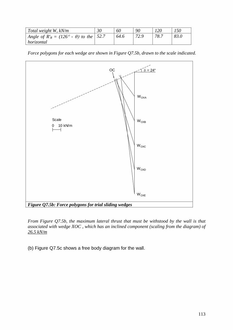
Force polygons for each wedge are shown in Figure Q7.5b, drawn to the scale indicated.

WOXA

WOXB

WOXC

WOXD

WOXE

δ = 24°OC

Scale0 10 kN/m

Figure Q7.5b: Force polygons for trial sliding wedges From Figure Q7.5b, the maximum lateral thrust that must be withstood by the wall is that associated with wedge XOC , which has an inclined component (scaling from the diagram) of 26.5 kN/m (b) Figure Q7.5c shows a free body diagram for the wall.

113

W

NT

26.5 kN/m

24°

Figure Q7.5c: Free body diagram for the wall The weight of the wall W is 3 m × b m × 24 kN/m3 = 72 b kN/m where b is the width of the wall (in m). Resolving forces vertically, N'B = W + 26.5 sin 24° B

Resolving forces horizontally, T'B = 26.5 cos 24° = 24.2 kN/m B

At failure, T'B, failure = N'B.tan 24° and we require T'B B = (N'BB.tan 24°) ÷ 2, hence (W + 26.5 sin 24°).tan24° = 48.4 kN/m ⇒ W + 10.78 = 108.71 kN/m ⇒ W = 72 b ≈ 98 kN/m ⇒ b ≈ 1.36 m (c) We would also have to check

• the adequacy of the factor of safety on soil strength or strength mobilization factor • safety against toppling • the bearing capacity of the base • structural adequacy of the wall • global stability (i.e. triggering a landslip) • provision for drainage of the backfill • possibility of accidental surcharge loading,

Q7.6 (a) Figure 7.52 shows a cross section through a masonry retaining wall, with a partially-sloping backfill which is subjected to a line-load of 100 kN/m as indicated. Use a graphical construction to estimate the lateral thrust which must be resisted by friction on the base of the wall, in order to prevent failure by the formation of a slip plane extending upward from the base of the wall, such as OA. (b) Is your answer likely to be greater or less than the true value, and why? (c) Suggest one way in which the ability of the wall to resist the thrust from the backfill could be improved.

114

[University of London 2nd year BEng (Civil Engineering) examination, Queen Mary and Westfield College] Q7.6 Solution (a) The soil/wall friction angle δ is given as 25° The succession of trial wedges is shown in Figure Q7.6a. The points A', A, B and C are marked off at horizontal distance intervals of 2 m.

Figure Q7.6a: Succession of trial wedges Each trial rupture line OA', OA etc makes an angle θA', θA etc to the horizontal such that tan θA' = (5.5 ÷ 2), tan θA = (6 ÷ 4), tan θB = (6 ÷ 6) etc. B

The retained soil is above the water table so we will assume zero pore water pressures. The forces acting on each wedge are



(iii) the effective stress reaction from the trial rupture, R'R, which acts at an angle of φ'crit (= 30°) to the normal to the rupture line with the shear component acting upwards (i.e., so as to resist sliding, i.e. at an angle of (90° - θ + φ'crit) = (120° - θ) to the horizontal (Figure Q7.6b)

(iv) For wedges OVB and beyond, the line load P = 100 kN/m acting vertically downward.

The area of each wedge is given by ½ × base × perpendicular height. For the wedges within the slope OVA' and OVA, the base length is the height of the wall = 5 m. For the wedges on the flat, the base is the horizontal distance AB or BC and the perpendicular height is the vertical distance to the level of the base of the wall, 6 m. Hence the areas and weights are as follows: Area OVA' = ½ × 5 m × 2 m = 5 m2; weight = 5 m2 × 20 kN/m3 = 100 kN/m

115

Area OVA = ½ × 5 m × 4 m = 10 m2; weight = 10 m2 × 20 kN/m3 = 200 kN/m Additional areas AOB, BOC etc = ½ × 2 m × 6 m = 6 m2; extra weight = 120 kN/m Hence Wedge OVA' OVA OVB OVC tanθ 5.5 ÷ 2 6 ÷ 4 6 ÷ 6 6 ÷ 8 θ, degrees 70.0 56.3 45.0 36.9 Total weight W, kN/m + P (= 100 kN/m) if applicable

100 200 320 + 100 440 + 100

Angle of R'R = (120° - θ) to the horizontal

50.0 56.3 75.0 83.1

Force polygons for each wedge are shown in Figure Q7.6b, drawn to the scale indicated. From Figure Q7.6b, the maximum lateral thrust that must be withstood by the wall is that associated with wedge VOB (which just includes the effect of the line load), which has a horizontal component (scaling from the diagram) of 98 kN/m (b) The answer is likely to be less than the true value, because

(i) we have assumed that the soil is on the verge of failure, which may not be the case in reality (if the soil is not at failure, it is not mobilising its full strength and the lateral thrust on the wall will be greater)

(ii) we have used a mechanism-based approach (“upper bound”): if we have chosen the wrong mechanism of failure, the answer will err on the unsafe side.

(c) The ability of the wall to resist sliding may be improved by

(i) increasing its weight (ii) embedding it slightly (iii) providing a shear key (iv) sloping the back of the wall

Note: assuming a unit weight for the concrete γconc = 24 kN/m3, the weight of the wall is 1.5 m × 5 m × 24 kN/m3 = 180 kN/m, and the available base friction of (180 kN/m + 98 kN/m × tan25° ) × tan25° = 105 kN/m is only just enough to prevent sliding, even taking into account the effect of the downward shear on the back of the wall (98 kN/m × tan25° ).

116

Figure Q7.6b: Force polygons for trial sliding wedges Q7.7 Figure 7.53 shows a cross section through a mass concrete retaining wall. Estimate the minimum lateral thrust which the wall must be able to resist to maintain the stability of the retained soil. Hence investigate the safety of the wall against sliding. [University of London 2nd year BEng (Civil Engineering) examination, King's College] Q7.7 Solution (a) The soil/wall friction angleδ is given as 25° The succession of trial wedges is shown in Figure Q7.7a. OB is 2.6 m up the slope; BC = CD = DE etc = 1.04 m up the slope.

117

Figure Q7.7a: Succession of trial wedges The area of each wedge OAB, OAC, OAD etc is given by ½ × base × perpendicular height = ½ × 5 m × (s.cos15°), where s (in m) is the upslope distance OB, OC etc and taking the baseline = 5 m as the back of the wall. Hence the areas and weights are as follows: Area OAB = ½ × 5 m × 2.6 m × cos15° = 6.28 m2; weight = 6.28 m2 × 20 kN/m3 = 125.6 kN/m Area OAC = ½ × 5 m × 3.64 m × cos15° = 10 m2; weight = 8.79 m2 × 20 kN/m3 = 175.8 kN/m Additional areas CAD, DAE etc are each ½ × 5 m × 1.04 m × cos15° = 2.5 m2; giving an extra weight of 50 kN/m Each trial rupture line OA, OB etc makes an angle θB, θB C etc to the horizontal scaled off the diagram. The forces acting on each wedge are



(iii) the effective stress reaction from the trial rupture, R'R, which acts at an angle of φ'crit (= 30°) to the normal to the rupture line with the shear component acting upwards (i.e., so as to resist sliding, i.e. at an angle of (90° - θ + φ'crit) = (120° - θ) to the horizontal

(iv) The pore water pressure reaction from the wall, = ½ × 2 m × 10 kN/m3 × 2 m = 20 kN/m acting horizontally (assuming hydrostatic conditions below the water table and taking the unit weight of water as 10 kN/m3)

118

(v) The pore water pressure reaction from the rupture, which has a horizontal component of 20 kN/m (because the water table is level, hence no horizontal flow) and hence has a magnitude of 20 ÷ sinθ kN/m acting perpendicular to the rupture surface, i.e. at an angle of (90° - θ) to the horizontal (Figure Q7.7b)

Hence Wedge OAB OAC OAD OAE OAF θ, degrees 66 59.5 54 49.5 46 Total weight W, kN/m 125 175 225 275 325 Angle of R'R = (120° - θ) to the horizontal

54 60.5 66 70.5 74

Force polygons for each wedge are shown in Figure Q7.7b, drawn to the scale indicated. From Figure Q7.7b, the maximum lateral thrust that must be withstood by the wall is that associated with wedge OAE , which (scaling from the diagram) has a horizontal component, including the pore water force of 78 + 20 = 98 kN/m The wall has weight 1.5 m × 5 m × 25 kN/m3 = 187.5 kN/m The downward force exerted on the wall by the soil is (78 kN/m × tan25° ) = 36 kN/m Assuming that the pore water pressure on the base of the wall varies linearly from 20 kPa at the heel (A) to zero at the toe, the pore water pressure upthrust on the base of the wall is ½ × 20 kPa × 2 m = 20 kN/m Thus the available friction on the base is (187.5 kN/m + 36 kN/m – 20 kN/m) × tan25° = 95 kN/m, which is insufficient to resist the imposed horizontal thrust of 98 kN/m.

119

Figure Q7.7b: Force polygons for trial sliding wedges Q7.8 (a) Figure 7.54a shows a cross-section through a gravity retaining wall retaining a partially sloping backfill of soft clay. By means of a graphical construction, estimate the minimum (active) lateral thrust that the wall must be able to resist in the short term. How does this compare with the maximum available sliding resistance on the base? (Assume that the limiting adhesion between the wall and the clay is equal to 0.4 × the undrained shear strength τu, and that the angle of soil/wall friction between the wall and the underlying sand is equal to 0.67×φ'.) (b) If the thrust from the backfill acts on the back of the wall at a distance of one-third of the height of the wall above the base, and the normal total stress distribution on the base is as shown in Figure 7.54b, calculate the values of σL and σR.

120

(c) What further investigations would you need to carry out, before the design of the wall could be considered acceptable? Q7.8 Solution (a) The succession of trial wedges is shown in Figure Q7.8a. The points A, B, C and D are marked off at horizontal distance intervals of 1.5 m. The horizontal distance from the line of the wall to A is 3 m.

Figure Q7.8a: Succession of trial wedges Each trial rupture line OA, OB etc makes an angle θA, θB etc to the horizontal such that tan θ

B

OA = (6 ÷ 3), tan θOB = (6 ÷ 4.5), tan θOC = (6 ÷ 6) etc. The retained soil is above the water table so we will assume zero pore water pressures. The forces acting on each wedge are

(i) the weight of the wedge, W, acting vertically downward (ii) the shear force TW on the soil/wall interface, which acts vertically and is given

by τw × lw = 0.5 × 25 kPa × 5 m = 50 kN/m. TR will be the same for all wedges (iii) the shear force TR on the rupture, which acts parallel to the rupture at an angle

q to the horizontal and is given by τu × lr = 25 kPa × lr where lr is the length of the rupture in m: lr

2 = 62 + xA2; lr

2 = 62 + xB2 etc where xA, xB etc are the

horizontal distances from the line of the wall to the point A, B etc. TB

R will be different for each wedge.

(iv) the normal reaction from the wall, NW, which acts horizontally but is unknown in magnitude (this is what we are trying to find)

(v) the normal reaction from the rupture, NR, which acts at right angles to the rupture, i.e. at an angle of (90° - θ) to the horizontal but is unknown in magnitude

121

(vi) For wedges OVC and beyond, the line load L = 150 kN/m acting vertically downward.

The area of each wedge is given by ½ × base × perpendicular height. For the wedge within the slope OVA, the base length is the height of the wall = 5 m and the perpendicular height is 3 m. For the wedges on the flat, OAB, BOC, COD etc, the base length is 6 m and the perpendicular height is 1.5 m. Hence the areas and weights are as follows: Area OVA = ½ × 5 m × 3 m = 7.5 m2; weight = 75 m2 × 20 kN/m3 = 150 kN/m Additional areas OAB, BOC, COD etc = ½ × 6 m × 1.5 m = 4.5 m2; extra weight = 90 kN/m Hence Wedge OVA OVB OVC OVD tanθ 6 ÷ 3 6 ÷ 4.5 6 ÷ 6 6 ÷ 7.5 θ, degrees 63.4 53.1 45.0 38.7 Total weight W, kN/m + L (= 150 kN/m) if applicable

150 240 330 + 150 420 + 150

Length of rupture lr = √{62 + xA2}

etc, m √{62+32} = 6.71

√{62+4.52} = 7.5

√{62+62} = 8.48

√{62+7.52} = 9.6

Shear force on rupture TR = 25 × lr, kN/m

168 187.5 212 240

Force polygons for each wedge are shown in Figure Q7.8b, drawn to the scale indicated. Note that NW is negative for OVB, and that OVA is not show. NW wuld also be negative for OVC in the absence of the line load.

122

Figure Q7.8b: Force polygons for trial sliding wedges From Figure Q7.8b, the maximum lateral thrust that must be withstood by the wall is that associated with wedge VOC including the effect of the line load, which is (by scaling from the diagram) 134 kN/m The maximum available sliding resistance due to friction on the base of the wall is given by Fmax = (W + TW) × tanδ = (360 + 50) × tan24° = 182.5 kN/m where W is the weight of the wall = 5 m × 3 m × 24 kN/m3 = 360 kN/m This is about 36% greater than the lateral thrust calculates, so the wall should be safe against sliding at least in the short term. (b) Figure Q7.8c shows a free body diagram of the wall and the forces and stresses acting on it (it is assumed that the basal shear stress TB takes the value needed to maintain horizontal equilibrium, 134 kN/m = NW, rather than the maximum of 182.5 kN/m calculated above)

123

Figure Q7.8c: Free body diagram for the retaining wall in Q7.8 Taking moments about O, {W × 1.5 m} + {TW × 3 m} – {NW × 5 m ÷ 3} = {σR × 3 m × 1.5 m} + {½(σL – σR) × 3 m × 1 m} ⇒ 540 + 150 – 223.33 = 3σR – 1.5.σL = 456.67 Vertical equilibrium gives W + TW = {σR × 3 m} + {½(σL – σR) × 3 m} ⇒ 360 + 50 = 1.5σR + 1.5.σL = 410 Adding these to eliminate σL gives 4.5σR = 866.67 kPa ⇒ σR = 192.6 kPa; σL = 80.7 kPa (c) we would also need to check

• the stability of the slope • the effect of a possible flooded tension crack • the bearing capacity of the sand at the base of the wall (check against bearing

failure) • the long term stability of the wall and the slope using long-term pore water

pressures and the effective stress failure criterion • the possibility of a global landslide • that excessive displacements would not occur

124

QUESTIONS AND SOLUTIONS: CHAPTER 8 Shallow foundations Q8.1 Figure 8.38 shows a cross section through a shallow strip footing. Estimate lower and upper bounds to the vertical load Q (per metre length) that will result in the rapid (undrained) failure of the footing. [University of London 2nd year BEng (Civil Engineering) examination, King's College] Q8.1 Solution Note: this question is rather trivial unless the formulae used are derived from first principles. This was expected of students in the examination, but the derivations are not repeated here. Lower boud solution based on frictionless stress discontinuities: use the reasoning in Section 8.2.2 (page 439) of the main text to derive Equation 8.3a, (σf – σ0) = 4.τu (8.3a) More advanced students might be expected to use the reasoning given in main text Section 9.5.2 (pages 507-508) to derive Equation 9.13, (σf – σ0) = (2 + π).τu (9.13) In the present case, τu = 35 kPa σ0 = 1 m × 18 kN/m3 = 18 kPa on either side of the footing Hence σf = (4 × 25 kPa) + 18kPa = 118 kPa using Equation 8.3a, or σf = (5.14 × 25 kPa) + 18kPa = 146.5 kPa using Equation 9.13 Multiplying by the foundation width 2 m, Q = 236 kN/m using the most conservative possible approach (Equation 8.3a; the answer using Equation 9.13 is 293 kN/m) Upper bound solution: use the reasoning in Section 8.3.1 (pages 439-443) of the main text to derive (σf – σ0) = 5.52.τu for a circular slip with its centre located above the centre of the footing (main text Figure 8.5). More advanced students might reasonably be expected to follow the reasoning given in main text Section 9.9.1(b) (pages 536-539) to derive Equation 9.47,

125

(σf – σ0) = (2 + π).τu (9.47) In the present case, with τu = 35 kPa and σ0 = 1 m × 18 kN/m3 = 18 kPa on either side of the footing σf = (5.52 × 25 kPa) + 18 kPa = 156 kPa using the slip circle mechanism, or σf = (5.14 × 25 kPa) + 18 kPa = 146.5 kPa using Equation 9.47 Multiplying by the foundation with 2 m, Q = 312 kN/m using the slip circle. (Equation 9.47 is the same as Equation 9.13: these upper and lower bounds are the same and the solution is therefore correct – provided of course that the conditions assumed in the analysis apply!) Q8.2 (a) Explain briefly the essential features of upper and lower bound plasticity analyses as applied to problems in geotechnical engineering. (b) A long foundation of depth D and width B is built on a clay soil of saturated unit weight γs, undrained shear strength τ u and frictional strength φ'. The water table is at a depth D below the soil surface. Show that the vertical load Q, uniformly distributed across the foundation, that will cause failure is given by (Q/B)≥(γ s.D + 4.τ u) in the short term, and by (Q/B)≥(K p

2γ s.D) in the long term, where K p is the passive earth pressure coefficient,

Kp =+−

11

sin 'sin '

φφ

(c) If γs = 20 kN/m3, τu = 25 kPa, φ' = 22° and D = 1.5 m, is the foundation safer in the short term or in the long term? [University of London 2nd year BEng (Civil Engineering) examination, Queen Mary and Westfield College] Q8.2 Solution (a) An upper bound is based on an assumed mechanism of collapse. If the assumed mechanism is incorrect, the analysis will err on the unsafe side. A lower bound solution is based on finding a system of stresses that can be in equilibrium with the applied loads without violating the failure criterion for the soil. It may be that a more efficient stress distribution exists, in which case the analysis will err on the safe side.

126

(b) Use the analyses given in main text Sections 8.2.2 (page 439) and 8.2.1 (pages 437-438) to derive the short term (undrained) and long term (effective stress) bearing capacities (σf – σ0) = 4.τu (8.3a) and (σ'f/σ'f 0) = Kp

2, where Kp = (1 + sinφ')/(1 - sinφ') (8.1) Substituting σf or σ'f = Q/B (Q is the load per metre length of the foundation) and (with zero pore water at depth D) σ0 or σ'0 = γs.D kPa, and noting that our answers are lower bounds to the actual failure loads, Q/B ≥ 4.τu + γs.D (short term), and Q/B ≥ Kp

2.γs.D (long term) (c) Substituting γs = 20 kN/m3, τu = 25 kPa, φ' = 22° and D = 1.5 m gives Kp = 2.197 and Q/B ≥ (4 × 25 kPa) + (20 kN/m3 × 1.5 m) = 130 kPa, short term Q/B ≥ (2.1972) × (20 kN/m3 × 1.5 m) = 145 kPa, long term Therefore the short term case is the more critical (this is usual with a foundation on a soft clay). Q8.3 A long concrete strip footing founded at a depth of 1 m below ground level is to carry an applied load (not including its own weight) of 300 kN/m. The soil is a clay, with undrained shear strength τu = 42 kPa, effective angle of friction φ' = 24°, and unit weight γ = 20 kN/m3. Calculate the width of the foundation required to give factors of safety on soil strength of 1.25 (on tanφ') and 1.4 (on τu). Both short-term (undrained) and long-term (drained) conditions should be considered. The water table is 1 m below ground level. Use Equation 8.9, with Nc = (2 + π), and a depth factor dc as given by Skempton (Table 8.2); and Equation 8.7, with Nq = Kp.eπtanφ' where Kp = (1+sinφ')/(1-sinφ'), with dq, Nγ, dγ and rγ as given by Meyerhof and Bowles (Table 8.1). Take the unit weight of concrete as 24 kN/m3. [University of Southampton 2nd year BEng (Civil Engineering) examination, slightly modified] Q8.3 Solution (a) Undrained case The design undrained design bearing capacity is given by main text Equation 8.9, (σf - σo)design = {Nc × sc× dc}× τu,design (8.9) with Nc = (2 + π) = 5.14; τu,design = 42 kPa ÷ 1.4 = 30 kPa and σo = γ.D = 20kN/m3 × 1m = 20kPa

127

From Table 8.2 (Skempton), the shape factor sc = 1 (because this is a long foundation with L >>B, whatever the value of B) and the depth factor dc = {1 + 0.23√(D/B)} assuming (D/B) ≤ 4. The foundation width B is as yet unknown. The actual pressure at the base of the foundation is 300 kN/m divided by the footing width B, i.e. (300/B) kPa, plus the pressure due to the concrete foundation, γconc.D = 24 kPa (D = 1 m; γconc= 24 kN/m3). Equating the actual and design base pressures, σf,design = [{Nc × sc× dc}× τu,design] + 20 kPa = 300/B + 24 kPa [5.14 × {1 + 0.23√(D/B)} × 30 kPa] + 20 kPa = 300/B + 24 kPa Solve by trial and error: with B = 1.7 m, D/B = 0.588 and the depth factor dc = 1.176. The left hand side of the equation (the design base pressure) is then numerically equal to 201.4 kPa; the right hand side (the actual base pressure) is 200.5 kPa, which is close enough. Thus the required foundation width for the short term case is approximately 1.7 m (b) Long term (effective stress) case The long term (drained) design bearing capacity is given by main text Equation 8.7, σ'f,design = {Nq×sq×dq}×σ'o + {Nγ×sγ×dγ×rγ×[0.5γB - u]} (8.7) with Nq = Kp.eπtanφ'des, Kp = (1+sinφ'des)/(1-sinφ'des),and dq, Nγ, dγ and rγ as given by Meyerhof and Bowles (Table 8.1). The design strength is now given by tanφ'des = (tan24°) ÷ 1.25 ⇒ φ'des = 19.6° φ'des =19.6°, Kp = 2.0096 and Nq = 6.151. From Table 8.1, sq = sγ = 1 (because L>>B) dq = dγ = 1 + 0.1 × (D/B) ×√Kp = 1 + 0.142D/B Nγ = (Nq – 1) × tan(1.4φ'des) = 5.151 × tan27.44° = 2.675 r γ = 1 - 0.25.log10(B/2) σ'o = γ.D = 20 kPa The pore water pressure u at a depth of B/2 below the bottom of the foundation = γw.B/2, so that [0.5γB - u] = 5B kPa (with B in metres)

128

The design effective stress on the base of the foundation is σ'f,design: σ'f,design = {Nq×sq×dq}×σ'o + {Nγ×sγ×dγ×rγ×[0.5γB - u]} or σ'f,design = {6.151 × (1 + 0.142D/B ) × 20 kPa}

+ {2.675 × (1 + 0.142D/B )× [1 - 0.25.log10(B/2]) × 5B} The pore water pressure acting on the base of the foundation is zero. The actual stress applied at the base of the foundation is 300 kN/m divided by the footing width B, i.e. (300/B) kPa, plus the stress due to the weight of the concrete foundation, γconc.D. The foundation width B must be chosen so that the actual and design stresses are the same. Equating the design and actual stresses, {6.151 × (1 + 0.142D/B ) × 20 kPa} + {2.675 × (1 + 0.142D/B )× [1 - 0.25.log10(B/2]) × 5B} = {(300/B) + 24 kPa} Solve by trial and error: with B = 2.18 m, D/B = 0.459, dq =dγ = (1 + 0.142D/B) = 1.065, and rγ = 0.99 so that the left hand side is numerically equal to {6.151 × 1.065 × 20 kPa} + {2.675 × 1.065× 0.99 × (5 × 2.18) kPa} = 161.8 kPa The right hand side is numerically equal to (300/2.18) + 24 = 161.6 kPa, which is near enough the same. Thus the required foundation width for the long term case is approximately 2.2 m Generally, it is unusual for the drained (long term) analysis to give a more critical result than the undrained (short term) analysis. Deep foundations Q8.4 Figure 8.39 shows a soil profile in which it proposed to install a foundation made up of a number of circular concrete piles of 1.5m diameter and 10m depth. Using the data given below, estimate the long-term allowable vertical load for a single pile, if a factor of safety of 1.25 on the soil strength tanφ' is required. (Assume that the horizontal effective stress at any depth is equal to (1-sinφ') times the vertical effective stress at the same depth, that the angle of friction δ between the concrete and the soil is equal to 0.67φ', and that the long-term pore water pressures are hydrostatic below the indicated water table. Take the unit weight of water as 10kN/m3, and the unit weight of concrete as 24kN/m3.) Data:

129

Bearing capacity factor = Kp.eπtanφ' × depth factor × shape factor, where Kp = (1+sinφ')/(1-sinφ') Depth factor = (1+0.2[D/B]) up to a limit of 1.5 Shape factor = (1+0.2[B/L]) and the foundation has width B, length L and depth D Comment briefly on the assumptions σ'h=(1-sinφ').σ'v and δ = 0.67φ'. Why in reality might it be necessary to reduce the allowable load per pile? [University of London 3rd year BEng (Civil Engineering) examination, Queen Mary and Westfield College, slightly modified] Q8.4 Solution In the sands & gravels, φ' = 30° and φ'des = tan-1{tan30°÷1.25} = 24.79°. The angle of soil/wall friction δdes = 0.67φ' des = 16.61°. In the clay, φ' = 20°; φ'des = tan-1 {tan20°÷1.25} = 16.23° and δdes = 10.88°. Note that the horizontal effective stresses are calculated as σ'h=(1-sinφ').σ'v using the full soil strength in each stratum, as to use the design soil strength would lead to increased values of σ'h and hence unduly optimistic increased values of skin friction shear stress τ. The skin friction shear stress τ = σ'h.tanδdes, and varies linearly between successive “key depths”, i.e. the soil surface, the water table, the interface between the sands & gravels and the clay, and the base of the pile. The skin friction shear stresses at these key depths are calculated as shown in Table Q8.4. The sands & gravels have saturated unit weight γ = 20 kN/m3; the clay has saturated unit weight γ = 18 kN/m3. In the sands & gravels, σ'h = (1-sinφ').σ'v with φ' = 30°, giving σ'h = 0.5 × σ'v. In the clays, σ'h = (1-sinφ').σ'v with φ' = 20°, giving σ'h = 0.658 × σ'v. Stratum Depth,

m σv, kPa = Σγ.z

u, kPa σ'v = σv – u, kPa

σ'h = (1-sinφ').σ'v kPa

δdes, ° τ = σ'h.tanδdes, kPa

S & G 0 0 0 0 0 16.61 0 S & G 2 40 0 40 20 16.61 5.97 S & G 5 100 30 70 35 16.61 10.44 Clay 5 100 30 70 46.1 10.88 8.86 Clay 10 190 80 110 72.4 10.88 13.92 Table Q8.4: Calculation of skin friction shear stresses at key depths The skin friction force over each section of the pile (0 – 2 m depth; 2 – 5 m depth; and 5 – 10 m depth) is given by the pile circumference × the pile section length × the average of the shear stresses at the top and bottom of the pile section. Hence the skin friction force is SF = [π × 1.5 m × 2 m × ½ × 5.97 kPa] + [π × 1.5 m × 3 m × ½ × (5.97 + 10.44) kPa] + [π × 1.5 m × 5 m × ½ × (8.86 + 13.92) kPa] = 28.13 kN + 116.0 kN + 268.37 kN = 412.5 kN The design base bearing effective stress is given by

130

σ'f,des = Kp × exp(π.tanφ'des) × depth factor dq × shape factor sq × σ'o σ'o is the in situ vertical effective stress at the depth of the base of the pile = 110 kPa. Kp × exp(π.tanφ'des) = {(1+sin16.23°)/(1 – sin16.23°)} × exp(π.tan16.23°) = 4.43 Pile depth D = 10 m, breadth (diameter) B = 1.5 m, Length (on plan, also the diameter) L = 1.5 m Hence D/B = 8.67 and B/L = 1 ⇒; shape factor sq = 1.2 and depth factor dq = 1.5 σ'f = 4.43 × 1.2 × 1.5 × 110 kPa = 877.14 kPa Area of pile = π × 1.52m2/4 = 1.767 m2

∴base bearing load = 877.14 kPa × 1.767 m2 = 1550 kN The upthrust on the base due to the pore water pressure is 80 kPa × 1.767 m2 = 141.4kN The design load is 412.5 kN (SF) + 1550 kN (BB) + 141.4 kN (pwp) = 2103.9 kN The weight of the foundation is (1.767 m2 × 10 m × 24 kN/m3) = 424.08 kN, giving a design applied load of 2104 kN – 424 kN = 1680 kN The in situ horizontal effective stress may well be higher than assumed by the use of σ'h = (1-sinφ').σ'h in the clay, especially if the clay is overconsolidated. In general, σ'h = (1-sinφ').σ'h is a conservative estimate, allowing perhaps for some reduction from the in situ value due to installation effects (see also the earlier note regading the use of unfactored soil strengths in calculating horizontal effective stresses). The friction angle δ between the pile and the soil is often assumed to be 0.67×φ' in coarse materials. In clays, however, particularly if the pile is rough, any failure surface will probably form in the soil, so that δ = 0.67.φ' is again conservative. However,the use of a bentonite slurry to support the pile bore during construction could reduce interface friction if a skin of bentonite remains between the pile and the soil. Interaction between closely spaced piles would probably reduce the ultimate load of n piles to less than n × the ultimate load of a single pile (due eg to a tendency to block failure). Slopes Q8.5 A partly-complete stability analysis using the Bishop routine method is given in the Table below. The configuration of the remaining slice (slice 4) and other relevant data are given in Figure 8.40. Abstract the necessary additional data from Figure 8.40, and determine the factor of safety of the slope for this slip circle.

131

Slice weight

w, kN/m

u.b, kN/m

φ'crit, ° nα × (w - u.b).tanφ'crit for Fs = 1.45, kN/m

1 390 0 25 196.5 2 635 90 25 251.8 3 691 163 25 235.1 4 ? ? 30 ? 5 472 130 30 198.9 6 236 20 30 137.7 [University of Southampton 2nd year BEng (Civil Engineering) examination, slightly modified] Q8.5 Solution The Bishop equation must be used in the form given in main text Equation 8.35(a):

( )( )∑∑⎪⎪⎭

⎪⎪⎬

⎫

⎪⎪⎩

⎪⎪⎨

⎧

⎟⎟⎟⎟

⎠

⎞

⎜⎜⎜⎜

⎝

⎛

+×−×=

s

critcrits

F

buww

Fαφ

αφ

α sin.'tancos

1'tan..sin.

1 (8.35a)

(Simplification to the form given in Equation 8.35(b) is not possible in this case, because the slices have different breadths b.)

Let ⎟⎟⎟⎟

⎠

⎞

⎜⎜⎜⎜

⎝

⎛

+s

crit

Fαφ

αsin.'tancos

1 = nα.

The solution procedure is as follows: 1. Assume a value of factor of safety Fs 2. Calculate the values of w, sinα, u.b and nα (which depends on Fs) for each slice 3. Determine whether Equation 8.35a is satisfied 4. If not, choose a new value of Fs 5. Repeat stages 2-4 until Equation 8.35a is satisfied The weight of slice 4 is approximately 5 m × {(6 m+7 m)/2} × 20 kN/m3 = 650 kN/m The pore water pressure at the left hand edge of slice 4 is approximately 5.4 m × 10 kN/m3 = 54 kPa. The pore water pressure at the right hand edge of slice 4 is approximately 4.6 m × 10 kN/m3 = 46 kPa. The average pore water pressure is therefore approximately 50 kPa, acting over a width b = 5 m, giving u.b = 250 kN/m. The remainder of the calculation for Fs = 1.45 is tabulated below (entries show in bold have been calculated)

132

Slice weight w, kN/m

α w.sinα kN/m

u.b, kN/m

φ'crit (w-ub)×tanφ’crit

nα for Fs=1.45

nα × (w - u.b).tanφ'crit for Fs = 1.45, kN/m

1 390 +46° 280.5 0 25° 181.9 1.080 196.5 2 635 +34° 355.1 90 25° 254.1 0.991 251.8 3 691 +22° 258.9 163 25° 246.2 0.955 235.1 4 650 +10° 112.9 250 30° 230.9 0.949 219.1 5 472 -8.2° -8.2 130 30° 197.5 1.007 198.9 6 236 -11° -45.0 20 30° 124.7 1.104 137.7 Table Q8.5a: trial slope stability calculation for Q8.5 For Fs=1.45, Σ{nα × (w - u.b).tanφ'crit} (i.e. the sum of the entries in the last column) = 1239.4 kN/m. Dividing this by Σ{w.sinα} = 954.1 kN/m, we obtain a calculated value of Fs (according to Equation 8.35a) of 1239.4 ÷ 954.1 = 1.299, compared with the assumed value of 1.45. The assumed value is therefore too high. Try Fs = 1.3: Slice weight

w, kN/m

α w.sinα kN/m

u.b, kN/m

φ'crit (w-ub)× tanφ’crit

nα for Fs=1.3

nα × (w - u.b).tanφ'crit for Fs = 1.3, kN/m

1 390 +46° 280.5 0 25° 181.9 1.050 191.0 2 635 +34° 355.1 90 25° 254.1 1.030 261.6 3 691 +22° 258.9 163 25° 246.2 0.942 231.9 4 650 +10° 112.9 250 30° 230.9 0.942 217.5 5 472 -8.2° -8.2 130 30° 197.5 1.008 199.1 6 236 -11° -45.0 20 30° 124.7 1.115 139.0 Table Q8.5b: second trial slope stability calculation for Q8.5 For Fs=1.3, Σ{nα × (w - u.b).tanφ'crit} (i. e. the sum of the entries in the last column) = 1240.1 kN/m. Dividing this by Σ{w.sinα} = 954.1 kN/m (as before), we obtain a calculated value of Fs of 1240.1 ÷ 954.1 = 1.3. This is the same as the assumed value of 1.3, hence Fs = 1.3 Q8.6 A slope failure can be represented by the four-slice system shown in Figure 8.41. By considering the equilibrium of a typical slice (resolving forces parallel and perpendicular to the local slip surface), and assuming that the resultant of the interslice forces is zero, show that the overall factor of safety of the slope Fs = tanφ'crit/tanφ'mob may be calculated as

133

( )[ ]( )∑

∑ −=

αφα

sin.'tan.cos.

wluw

F crits

where the symbols have their usual meaning. If the pore pressure conditions which caused failure of the slope shown in Figure 8.41 can be represented by average pore water pressures of 15kPa, 60kPa, 70kPa and 40kPa on AB, BC, CD and DE respectively, estimate the value of φ'crit along the failure surface DE. [University of Southampton 2nd year BEng (Civil Engineering) examination, slightly modified] Q8.6 Solution A free body diagram showing the forces acting on each of the four slices, ignoring the inter-slice forces, is given in Figure Q8.6. Resolving parallel to the base of an individual slice, assuming the inter-slice forces are zero, T = w.sinα Resolving perpendicular to the base of an individual slice (again assuming that the interslice forces are zero), N = w.cosα where α is taken as positive when the base of the slice slopes up from bottom right to top left (i.e. slices 1,2 and 3)

Figure Q8.6: Free body diagram showing the forces acting on each of the four slices For each slice, T = (N-U).tanφ'mob = {(N-U).tanφ'crit}/Fs where Fs = tanφ'crit/tanφ'mob

134

The pore water force U acting on the base of a slice is equal to the average pore water pressure u × the base length l. Hence for each slice, T = w.sinα = {(w.cosα - u.l).tanφ'crit}/Fs, or

( )α

φαsin.

'tan..cos.w

luwF crits

−=

The overall factor of safety Fs for the system is given by

( )[ ]( )∑

∑ −=

αφα

sin.'tan..cos.

wluw

F crits

For each slice in the four slice system shown in Figure 8.41, the values of b, w, α, w.sinα, w.cosα,, u.l and (w.cosα - u.l).tanφ'crit (="NUM") are tabulated below: Slice b, m w,

kN/m α wsinα

kN/m wcosα kN/m

l, m u, kPa

u.l, kN/m

φ'crit NUM kN/m

1 8 640 47° 468.1 436.5 11.73 15 176.0 20° 94.8 2 25 5750 25° 2430.1 5211.3 27.58 60 1654.8 25° 1658.4 3 14 3640 12° 756.8 3560.5 14.31 70 1001.7 25° 1193.2 4 16 1920 -5° -167.3 1912.7 16.06 40 642.4 φ'DE 1270.3

×tanφ'DE Table Q8.6: second trial slope stability calculation for Q8.6 In calculating w for slice 2, it is necessary to take account of the different unit weights of the two soil types present. The base length l of each slice is equal to b/cosα, where b is the slice width. As the system is at failure, Fs = 1. Hence Σw.sinα = Σ{(w.cosα - u.l).tanφ'crit} = Σ{NUM} From the table, Σw.sinα = 3487.7 kN/m, and Σ{(w.cosα - u.l).tanφ'crit} = Σ{NUM} = 2946.4 + 1270.3.tanφ'DE kN/m. Hence 3487.7 = 2946.4 + 1270.3.tanφ'DE

135

⇒ tanφ'DE = 541.3 ÷ 1270.3 ⇒ φ'DE = 23°

136

QUESTIONS AND SOLUTIONS: CHAPTER 9 Bearing capacity of foundations Q9.1. Figure 9.30 shows a cross-section through the bottom of an under-reamed pile in a clay of undrained shear strength τu = 75 kPa. By considering the stress state of the soil in the zones immediately below the base of the pile and immediately above the "bell" of the under-ream, estimate the bearing capacity factor N c = (σf - σ 0)/τ u. (Note: the shear stress on the base of the pile must be zero, but what is the effect of shear stress τw between the top of the "bell" of the under-ream and the adjacent soil?). Comment on the shortcomings of your solution. Q9.1 Solution Let Zone 1 be the soil immediately above the bell on the right hand side of the under-ream; and let Zone 2 be below the base of the pile. The vertical stress below the base of the pile is σf, and the associated shear stress (acting on the horizontal plane) is zero. The Mohr circle of stress for Zone 2 is shown in Figure Q9.1a.

σf = s2 + su

τ

σ

su

s2σf

Figure Q9.1a: Mohr circle of total stress for Zone 2, the soil immediately below the pile base The average total stress in Zone 2 is s2 = σf – τu and the direction of the major principal total stress is vertical, i.e the major principal total stress acts on the horizontal plane. For Zone 1, let us first assume that there is no shear stress on the upper surface of the bell, so that the normal stress (= σ0) is a principal stress. The corresponding Mohr circle is shown in Figure Q9.1b.

137

s1 = σ0 + su

τ

σ

su

s1σ0

Figure Q9.1b: Mohr circle of total stress for Zone 1, the soil immediately above the bell, assuming zero interface shear stress (τw = 0) The average total stress in Zone 1 is s1 = σ0 +τu σ0 is the minor principal total stress: the major principal total stress therefore acts parallel to the top of the bell, i.e. on a plane at an angle of 30° to the horizontal. The rotation in the direction of the major principal total stress between Zones 1 and 2 is (180° + 30°) = 210° = (7π/6) radian (see Figure Q9.1c).

Fan zoneθ = 210º

Figure Q9.1c: Rotation of plane of major principal total stress between Zones 1 and 2 (τw = 0) Hence s2 – s1 = (2.τu.θ) = (14π/6)τu ⇒ s2 = s1 + (7π/3)τu σf = s2 + τu and s1 = σ0 +τu ⇒ σf = σ0 +τu + (7π/3)τu +τu ⇒ Nc = (σf - σ0)/τu = ( 2 + 7π/3) = 9.33

138

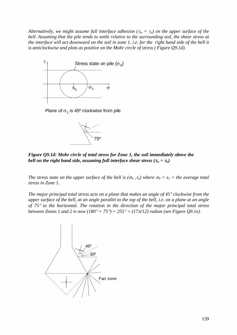
Alternatively, we might assume full interface adhesion (τw = τu) on the upper surface of the bell. Assuming that the pile tends to settle relative to the surrounding soil, the shear stress at the interface will act downward on the soil in zone 1, i.e. for the right hand side of the bell it is anticlockwise and plots as positive on the Mohr circle of stress ( Figure Q9.1d).

τ

σ

Stress state on pile (σ0)

s1 σ1

Plane of σ1 is 45º clockwise from pile

75º

Figure Q9.1d: Mohr circle of total stress for Zone 1, the soil immediately above the bell on the right hand side, assuming full interface shear stress (τw = τu) The stress state on the upper surface of the bell is (σ0 ,τu) where σ0 = s1 = the average total stress in Zone 1. The major principal total stress acts on a plane that makes an angle of 45° clockwise from the upper surface of the bell, at an angle parallel to the top of the bell, i.e. on a plane at an angle of 75° to the horizontal. The rotation in the direction of the major principal total stress between Zones 1 and 2 is now (180° + 75°) = 255° = (17π/12) radian (see Figure Q9.1e).

Fan zone

30º

45º

139

Figure Q9.1e: Rotation of plane of major principal total stress between Zones 1 and 2 (τw = τu) Hence s2 – s1 = (2.τu.θ) = (17π/6)τu ⇒ s2 = s1 + (17π/6)τu σf = s2 + τu and s1 = σ0 ⇒ σf = σ0 + (17π/6)τu +τu ⇒ Nc = (σf - σ0)/τu = ( 1 + 17π/6) = 9.9 Thus the shear stress on the upper surface of the under-ream bell makes little difference to the bearing capacity factor expressed in this way. The main shortcomings of the solution are that

i. we don’t know the value of σ0 (although σ0 → 0 if a gap opens up) ii. a full lower bound solution would require us to demonstrate that the stress field

could be continued to infinity without violating the failure condition iii. the weight of the soil has been neglected

Retaining walls and earth pressures Q9.2. By considering Mohr circles of stress for zones of soil adjacent to the retaining wall and immediately below the free soil surface, deduce an expression for the active earth pressure coefficient σ'h/(γz-u) behind a retaining wall in a soil having an effective angle of friction φ', where the angle of soil/wall friction is δ and the retained soil surface is level. Q9.2 Solution Let Zone 1 be the soil immediately adjacent to the retaining wall; and let Zone 2 be immediately below the retained soil surface (Figure Q9.2a).

2

1

Figure Q9.2a: Definition sketch Zone 2 is a conventional active zone, with (at depth z), σ'v = γ.z – u and

140

σ'h = [(1 - sin φ')/(1 + sinφ')].σ'v The Mohr circle of effective stress for Zone 2 is shown in Figure Q9.2b.

σ’h

τ

σ’s’2 σ’v

φ’

Figure Q9.2b: Mohr circle of effective stress for Zone 2, the soil immediately below the retained surface The average effective stress in Zone 2, s'2 , is given by σ'v = s'2 + t2 = s'2. (1 + sin φ') ⇒ s'2 = σ'v /(1 + sin φ') and the direction of the major principal effective stress is vertical, i.e the major principal effective stress acts on the horizontal plane. In Zone 1, the soil tends settle relative to the retaining wall, so that, the shear stress at the interface will act upward on the soil, i.e. it is anticlockwise for the wall as shown and plots as positive on the Mohr circle of stress. The stress state on the interface (τw ,σ'h,w) is given by (τw/σ'h,w) = tanδ where δ is the angle of soil/wall friction, and σ’w is less than the average effective stress in zone 1 (s'1) because this is an active pressure problem with the horizontal stress reducing towards the wall. The Mohr circle for Zone 1 is shown in Figure Q9.2c.

σ’h

τ

σ’s’1 σ’v

δ

Δ−δ

Δ+δ

180º-2Δ

ΔΔ

Stress stateon wall

Figure Q9.2c: Mohr circle of effective stress for Zone 1, the soil immediately behind the wall

141

From the geometry of the Mohr circle for Zone 1, t1/sinδ = s'1/sinΔ, where sinΔ = sinδ/(t1/s'1) = sinδ/sinφ' and the plane on which the major principal effective stress acts in Zone 1 is ½(180° - 2Δ + Δ + δ) = 90° - (Δ - δ)/2 clockwise from the vertical (see main text pages 499 – 501). The rotation in the direction of the major principal effective stress, θ, between zones 1 and 2 is therefore θ = (Δ - δ)/2 (Figure Q9.2d)

(Δ−δ)/2

Plane of σ’1in zone 1

Plane of σ’1in zone 2

Figure Q9.2d: Orientations of planes on which the major principal effective stresses act in Zones 1 and 2 Hence s'2/s'1 = exp(2θ.tanφ') = exp[(Δ – δ).tanφ'] From Figure Q9.2b , s'2 = (γz – u)/(1 + sin φ') and (from Figure Q9.2c), σ'h,w = s'1 – t1.cos(Δ – δ) = s'1.(1 – sinφ'.cos(Δ – δ))

⇒ ( )( )[ ] ( )[ ]

[ ]'sin1'tan.exp.cos'.sin1

uz'

K w,ha φ

φδΔδΔφγσ

+−−−−

=−

=

Q9.3. Figure 9.31 shows a cross section through a thrust block, which relies on the pressure of the soil behind it to resist an imposed lateral thrust P whose value is 2.5 smaller than that which would cause passive failure. Estimate the maximum allowable value of P if the width of the thrust block is 3m, and its back is smooth. (Ignore the effect of shear stresses on the base of the thrust block and three-dimensional effects.) If the back of the thrust block is rough, with an angle of interface friction δ, show, by considering Mohr circles of stress at a depth z in zones of soil adjacent and away from the thrust block, that the earth pressure coefficient K p (= σ'v/[γz-u]) is given by

142

Kp = {[1+sinφ'cos(Δ+δ)]/[1-sinφ']}×e{(Δ+δ)tanφ'} where sinΔ = sinδ/sinφ'. Hence calculate the maximum allowable value of P if δ=φ'. (It may be assumed without proof that the ratio of average principal effective stress between two uniform stress zones separated by a fan zone of included angle θ is given by s'2/s'1 = exp{2θtanφ'}, and that the rotation of the direction of major principal effective stress is θ.) [3rd year BEng civil engineering examination, University of London (Queen Mary & Westfield College)] Q9.3 Solution In the absence of interface friction, the horizontal thrust P that would cause failure is calculated as follows. At 4 m depth, the vertical effective stress (assuming zero pore water pressures) is σ'v = 4 m × 20 kN/m3 = 80 kPa. The passive earth pressure coefficient for a frictionless wall is Kp = (1 + sinφ')/(1 - sinφ') and for φ' = 30°, Kp = 1.5 ÷ 0.5 = 3 Hence the horizontal total stress acting on the wall at 4 m depth = 3× 80 kPa = 240 kPa, and the total lateral thrust P at failure is Pf = ½× 240 kPa × 4 m × 3m = 1440 kN and the allowable thrust Pallowable = Pf ÷ 2.5 = 576 kN Now assume that the back of the thrust block is rough, with an interface friction angle δ. Let Zone 1 be the soil immediately below the retained soil surface, and let Zone 2 be adjacent to the thrust block (Figure Q9.3a).

Figure Q9.3a: Definition sketch Zone 1 is a conventional passive zone, with (at depth z),

143

σ'v1 = γ.z – u and σ'h1 = [(1 + sin φ')/(1 - sinφ')].σ'v1 The Mohr circle of effective stress for Zone 1 is shown in Figure Q9.3b.

Figure Q9.3b: Mohr circle of effective stress for Zone 1, the soil immediately below the free surface The average effective stress in Zone 1, s'1 , is given by s'1 = σ'v1 + t1 = σ'v1 + s'1 .sin φ' ⇒ s'1 = σ'v1 /(1 - sin φ') and the direction of the major principal effective stress is horizontal, i.e the major principal effective stress acts on the vertical plane. In Zone 2, the soil tends to move up relative to the thrust block, so that the shear stress at the interface will act downward on the soil, i.e. it is clockwise for the wall as shown and plots as negative on the Mohr circle of stress. The stress state on the thrust block (τw ,σ'h,w) is given by (τw/σ'h,w) = - tanδ where δ is the angle of interface friction, and σ’w is greater than the average effective stress in zone 2 (s'2) because this is a passive pressure problem with the horizontal stress decreasing away from the thrust block. The Mohr circle for Zone 2 is shown in Figure Q9.3c.

144

Figure Q9.3c: Mohr circle of effective stress for Zone 2, the soil immediately behind the thrust block From the geometry of the Mohr circle for Zone 2, t2/sinδ = s'2/sinΔ, where sinΔ = sinδ/(t2/s'2) = sinδ/sinφ' and the plane on which the major principal effective stress acts in Zone 2 is ½(Δ + δ) anticlockwise from the vertical (see main text pages 499 – 501). The rotation in the direction of the major principal effective stress, θ, between zones 1 and 2 is therefore θ = (Δ + δ)/2 (Figure Q9.3d)

(Δ+δ)/2

Plane of σ’1in zone 1Plane of σ’1

in zone 2

Figure Q9.3d: Orientations of planes on which the major principal effective stresses act in Zones 1 and 2 Hence s'2/s'1 = exp(2θ.tanφ') = exp[(Δ +δ).tanφ'] From Figure Q9.3b , s'1 = (γz – u)/(1 - sin φ')

145

and (from Figure Q9.3c) σ'h,w = s'2 + t2.cos(Δ + δ) = s'2.(1 + sinφ'.cos(Δ + δ))

⇒ ( )( )[ ] ( )[ ]


uz'

K w,hp φ

φδΔδΔφγσ

−+++

=−

=

If δ = φ' = 30°, Δ = 90°; (Δ + δ) = 120° = 2π/3

[ ]

[ ] 026.530sin1

30tan.3

2exp.120cos.30sin1K p =

°−

⎥⎦

⎤⎢⎣

⎡°⎟

⎠⎞

⎜⎝⎛°°+

=

π

and Pallowable = 576 kN × 5.026 ÷ 3 = 965 kN Q9.4. (a) A bulldozer has a blade 2.5m wide. Estimate the total force on the bulldozer blade when it is used to move a 1.5m high bank of dry sand which has φ' = 30° and unit weight γ = 18 kN/m3, if the angle of friction between the sand and the bulldozer blade is 15°. (b) If this is 85% of the maximum force the bulldozer can provide, estimate the maximum depth of clay of undrained shear strength τu = 80 kPa that the bulldozer could move, assuming that the adhesion between the clay and the bulldozer blade is 0.5τu and that the depth of the blade is 1.6 m. (Note: conditions in front of the bulldozer blade will be passive in both cases). Q9.4 Solution (a) Let Zone 1 be the soil immediately below the free soil surface, and let Zone 2 be adjacent to the bulldozer blade (Figure Q9.4a).

2

1

Figure Q9.4a: Definition sketch Zone 1 is a conventional passive zone, with (at depth z), σ'v1 = γ.z – u and

146

σ'h1 = [(1 + sin φ')/(1 - sinφ')].σ'v1 The Mohr circle of effective stress for Zone 1 is shown in Figure Q9.4b.

σ’v

τ

σ’s’1 σ’h

φ’

Figure Q9.4b: Mohr circle of effective stress for Zone 1, the soil immediately below the free surface The average effective stress in Zone 1, s'1 , is given by s'1 = σ'v1 + t1 = σ'v1 + s'1 .sin φ' ⇒ s'1 = σ'v1 /(1 - sin φ') and the direction of the major principal effective stress is horizontal, i.e the major principal effective stress acts on the vertical plane. In Zone 2, the soil tends to move up relative to the bulldozer blade, so that the shear stress at the interface will act downward on the soil, i.e. it is clockwise for the problem as drawn and plots as negative on the Mohr circle of stress. The stress state on the bulldozer blade (τw ,σ'h,w) is given by (τw/σ'h,w) = - tanδ where δ is the angle of interface friction, and σ’w is greater than the average effective stress in zone 2 (s'2) because this is a passive pressure problem with the horizontal stress decreasing away from the bulldozer blade. The Mohr circle for Zone 2 is shown in Figure Q9.4c.

147

σ’v

τ

σ’s’2

σ’hδ

Δ+δ

180º-2Δ

ΔΔ

Stress stateon dozer blade

φ’

Figure Q9.4c: Mohr circle of effective stress for Zone 2, the soil immediately in front of the bulldozer blade From the geometry of the Mohr circle for Zone 2, t2/sinδ = s'2/sinΔ, where sinΔ = sinδ/(t2/s'2) = sinδ/sinφ' and the plane on which the major principal effective stress acts in Zone 2 is ½(Δ + δ) anticlockwise from the vertical (see main text pages 499 – 501). The rotation in the direction of the major principal effective stress, θ, between zones 1 and 2 is therefore θ = (Δ + δ)/2 (Figure Q9.4d)

(Δ+δ)/2

Plane of σ’1in zone 1Plane of σ’1

in zone 2

Figure Q9.4d: Orientations of planes on which the major principal effective stresses act in Zones 1 and 2 Hence s'2/s'1 = exp(2θ.tanφ') = exp[(Δ +δ).tanφ']

148

From Figure Q9.4b , s'1 = (γz – u)/(1 - sin φ') and (from Figure Q9.4c) σ'h,w = s'2 + t2.cos(Δ + δ) = s'2.(1 + sinφ'.cos(Δ + δ))

⇒ ( )( )[ ] ( )[ ]


uz'

K w,hp φ

φδΔδΔφγσ

−+++

=−

=

If φ' = 30° and δ = 15°, Δ = 31.174° and (Δ + δ) = 46.17° = 0.806 radian

[ ] [[ ]

]288.4

30sin130tan.806.0exp.17.46cos.30sin1K p =

°−°°°+

=

and the force on the blade F = ½ × (4.288 × 18 kN/m3 × 1.5 m) × 1.5 m × 2.5 m = 217 kN (b) This is 85% of the maximum force the bulldozer can exert. Therefore, Fmax = 217.06 kN ÷ 0.85 = 255.37 kN To find the maximum depth of clay of undrained shear strength τu = 80 kPa that the bulldozer could move, we must repeat the analysis using the undrained shear strength (τmax = τu) failure criterion. As before, let Zone 1 be the soil immediately below the free soil surface, and let Zone 2 be adjacent to the bulldozer blade (Figure Q9.4a). Zone 1 is a conventional passive zone, with (at depth z), σv1 = γ.z; σh1 = γ.z + 2.τu; and s1 =σv1+τu The Mohr circle of total stress for Zone 1 is shown in Figure Q9.4e.

σv

τ

σs1 σh

τu

Figure Q9.4e: Mohr circle of total stress for Zone 1, the soil immediately below the free surface

149

The direction of the major principal total stress is horizontal, i.e the major principal total stress acts on the vertical plane. In Zone 2, the soil tends to move up relative to the bulldozer blade, so that the shear stress at the interface will act downward on the soil, i.e. it is clockwise for the problem as drawn and plots as negative on the Mohr circle of stress. The stress state on the bulldozer blade (σh,w, τw) is given by τw = -0.5.τu where σh,w is greater than the average total stress in Zone 2 (s2) because this is a passive pressure problem with the horizontal stress decreasing away from the bulldozer blade. The Mohr circle of total stress for Zone 2 is shown in Figure Q9.4f.

τ

σs2

τu

Stress stateon dozer blade

Δ

Figure Q9.4f: Mohr circle of total stress for Zone 2, the soil immediately in front of the bulldozer blade From the geometry of the Mohr circle for Zone 2, sinΔ = (0.5.τu)/τu = 0.5 and the plane on which the major principal total stress acts is Δ/2 anticlockwise from the vertical (see main text pages 501 – 502). The rotation in the direction of the major principal effective stress, θ, between zones 1 and 2 is therefore θ = Δ /2 (Figure Q9.4g)

150

Δ/2

Plane of σ1in zone 1Plane of σ1

in zone 2

Figure Q9.4g: Orientations of planes on which the major principal total stresses act in Zones 1 and 2 Hence s2 – s1 = 2.τu.θ = Δ.τu From Figure Q9.4e , s1 =σv1+τu and (from Figure Q9.4f) σh,w = s2 + τu.cosΔ ⇒ σh,w = σv1+τu + Δ.τu + τu.cosΔ = σv1+τu. (1 + Δ.+ cosΔ) With Δ = sin-1(0.5) = 30° = π/6 radian, σh,w = σv1+ 2.39.τu At the free soil surface, σv1 = 0 and σh,w = 2.39.τu. At a depth h, σv1 = γ.h and σh,w = γ.h + 2.39.τu. Thus the average horizontal stressacting over the depth h is γ.h/2 + 2.39.τu, and the force F is given by F = (γ.h/2 + 2.39.τu) × h × 2.5 m = 255.37 kN Assume that the unit weight of the soil γ is the same as before (= 18 kN/m3), and taking τu = 80 kPa, h (in metres) is given by the solution of (478.h + 22.5.h2) = 255.37 kN

h = ( )

5.2225.2237.2554478478 2

×××+±−

⇒ h = 0.52 m

151

QUESTIONS AND SOLUTIONS: CHAPTER 10 Retaining walls Q10.1 Figure 10.33 shows the idealized geometry of a proposed retaining wall, together with soil and groundwater conditions. (a) Estimate the long-term pore water pressure distribution, due to steady-state seepage around the wall. (b) Using the idealized soil profile, calculate the depth of embedment required for the wall to be just stable in the long term and the corresponding prop load. (c) Explaining your method, estimate the design depth of embedment of the wall and the associated prop load. All soils have unit weight 20 kN/m3. Take the unit weight of water as 10 kN/m3. The upper sands and gravels have φ'crit = 30° and φ'peak = 34°, the clays have φ'crit = 20° and φ'peak = 22°, and the lower sands have φ'crit = 32° and φ'peak = 36°. Use the earth pressure coefficients given in Tables 7.6 and 7.7. Q10.1 Solution (a) Following construction, the groundwater level in front of the wall must be drawn down to formation level (3.25m AOD) to prevent flooding. Take Ordnance Datum (OD) as the datum for the measurement of total head. Behind the wall, the head at the top of the clays in the idealized cross section (Figure 10.33c) is 10.6m. In front of the wall, the head at formation level is 3.25m AOD. It is reasonable to assume that the head drop of (10.6 m - 3.25m) = 7.35 m takes place as the groundwater flows through the clay, because it is of much lower permeability than the upper sands and gravels and the lower sands. Assume that the water table levels in the two aquifers remain unchanged, and also (as is likely) that the wall penetrates to below the base of the clay. In the clay behind the wall, the pore water pressures will be the same as they were prior to construction, i.e. corresponding to a drop in head that is linear with depth from 10.6 m AOD at the top (u = 32 kPa) to 5.7 m AOD at the base (u = 105 kPa). In the clay in front of the wall, the drop in head will be linear with distance upward from the base of the stratum, from 5.7 m AOD at the base (u = 105 kPa) to 3.25 m AOD at the upper (excavated) surface (u = 0). The pore water pressures at key depths are given in Table Q10.1b. The corresponding pore water pressure distribution is sketched in Figure Q10.1a.

152

Figure Q10.1a: long term pore water pressure distribution around the wall (b) Calculate the depth of embedment required for the wall to be just stable on the basis of active pressures being developed in the soil behind the wall and passive pressures in front. (Note this does not quite correspond to rigid body rotation about the prop, because rigid body rotation about the prop would imply the development of passive pressures in the retained soil above prop level. The assumption of fully active conditions behind the wall is justified because a sudden transition from passive to active at prop level would be unrealistic, and because an overall forward movement of the wall is almost certain to occur in practice). Use earth pressure coefficients based on critical state strengths and full wall friction (δ = φ'crit), taken from Tables 7.6 and 7.7: Stratum φ'crit Ka (δ = φ'crit) Kp (δ = φ'crit) Upper sands & gravels

30° 0.2661 5.6704

Clays 20° 0.4129 2.8608 Lower sands 32° 0.2431 6.6432 Table Q10.1a: Active and passive earth pressure coefficients based on critical state strengths and wall friction δ = φ’crit

153

The vertical total stresses σv, pore water pressures u, values of (σv - u), and horizontal effective stresses σ'h = Ka×(σv - u) (active) or σ'h = Kp×(σv - u) (passive) at key depths behind and in front of the wall are given in Table Q10.1b. Behind wall Level, mAOD

Depth below OGL, m

Stratum σv, kPa u, kPa (σv - u), kPa

σ'h, kPa = Ka×(σv - u)

14.85 0 Upper sands & gravels

0 0 0 0

10.6 4.25 Upper sands & gravels

85 0 85 22.619


149 32 117 31.134

7.4 7.45 Clays 149 32 117 48.309 -4.8 19.65 Clays 393 105 288 118.915 -4.8 19.65 Lower sands 393 105 288 70.013 3.25 - x 11.6+x Lower sands (11.6+

x) × 20 (2.45+x) × 10

207.5 + 10x

50.443 + 2.43x

In front of wall Level, mAOD

Depth below dredge, m


σ'h, kPa = Kp×(σv - u)

3.25 0 Clays 0 0 0 0 -4.8 8.05 Clays 161 105 56 160.205 -4.8 8.05 Lower sands 161 105 56 372.019 3.25 - x x Lower sands 20x (2.45+x)

× 10 10x - 24.5

66.43x – 162.76

Table Q10.1b: Vertical and horizontal stresses and pore water pressures at key depths behind and in front of the wall, for calculation of conditions at collapse The active and passive stress and pore water pressure blocks are as shown in Figure Q10.1b. The resultant forces and lever arms are given in Table Q10.1c.

154

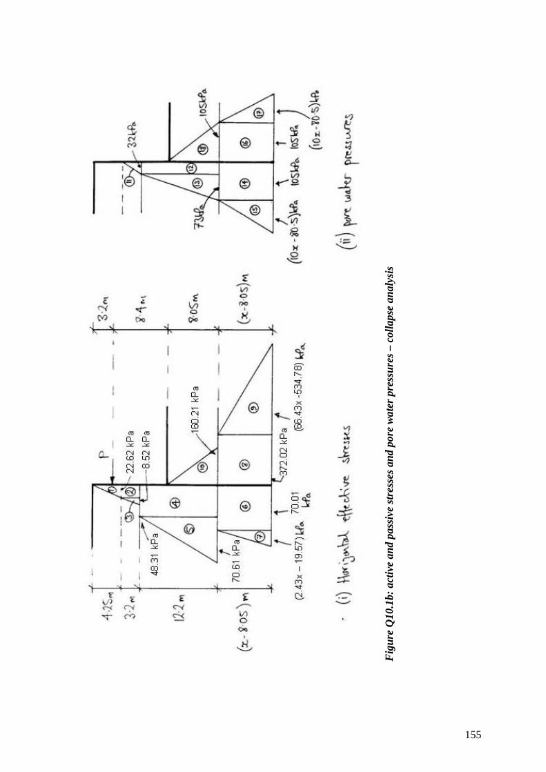
Fig

ure

Q10

.1b:

act

ive

and

pass

ive

stre

sses

and

por

e w

ater

pre

ssur

es –

col

laps

e an

alys

is

155

Behind wall (Forces acting left to right; moment clockwise about toe) Stress block (see Fig Q10.1b)

Resultant force, kN/m Lever arm about toe of wall, m

1 0.5 × 22.619(kPa) × 4.25(m) x + 7.35 + (4.25÷3) 2 22.619(kPa) × 3.2(m) x + 4.15 + (3.2÷2) 3 0.5 × 8.515(kPa) × 3.2(m) x + 4.15 + (3.2÷3) 4 48.309(kPa) × 12.2(m) x - 8.05 + (12.2÷2) 5 0.5 × 70.606(kPa) × 12.2(m) x - 8.05 + (12.2÷3) 6 70.013(kPa) × (x - 8.05)(m) (x - 8.05)÷2 7 0.5× (2.43x - 19.57)(kPa)

× (x - 8.05) (m) (x - 8.05)÷3

11 0.5 × 32(kPa) × 3.2(m) x + 4.15 + (3.2÷3) 12 32(kPa) × 12.2(m) x - 8.05 + (12.2÷2) 13 0.5 × 73(kPa) × 12.2(m) x - 8.05 + (12.2÷3) 14 105(kPa) × (x - 8.05) (m) (x - 8.05)÷2 15 0.5 × (10x - 80.5) (kPa)

× (x - 8.05) (m) (x - 8.05)÷3

In front of wall (Forces acting right to left; moment anticlockwise about toe) Stress block (see FigQ10.1b)

Resultant force Lever arm about toe of wall

8 372.019(kPa) × (x - 8.05) m (x - 8.05) ÷ 2 9 0.5 × (66.43x – 534.779)(kPa) ×

(x - 8.05)(m) (x - 8.05)÷3

10 0.5 × 160.205(kPa) × 8.05(m) (x - 8.05) + (8.05÷3) 16 105(kPa) × (x - 8.05) m (x - 8.05)÷2 17 0.5 × (10x - 80.5)(kPa) ×

(x - 8.05) m (x - 8.05)÷3

18 0.5 × 105(kPa) × 8.05(m) (x - 8.05) + (8.05÷3) Prop load P 8.4 + x Table Q10.1c: Forces and lever arms about the toe of the wall for the stress and pore water pressure blocks shown in Figure Q10.1b (collapse calculation) Note: it is assumed that the wall penetrates into the lower sands, i.e. x ≥ 8.05m. Also, the pore water pressures in the lower sands are the same on both sides of the wall (pressure blocks 14 and 15 behind the wall; pressure blocks 16 and 17 in front), and could be omitted from the equilibrium calculation because they cancel each other out. Assembling the equations of horizontal force (ΣF=0) and moment (ΣM=0) equilibrium onto a spreadsheet and solving by trial and error, we obtain x ≈ 9.2 m; P ≈ 582 kN/m (c) The design calculation will be carried out generally in accordance with BS8002. Thus

156

(i) A surcharge of 10 kPa must be applied to the retained soil surface: this will increase the vertical and horizontal pressures at each of the key depths behind the wall (as indicated in Table Q10.1e) and introduce an additional rectangular stress block (labelled 0 in Figure Q10.1c)

(ii) The depth of the excavation must be increased by the smaller of (a) 10% of the retained height, i.e. 1.16 m, and (b) 0.5 m. Thus the design depth of excavation is increased by 0.5 m to 12.1 m, giving a design formation level of 2.75 m AOD

(iii) The design earth pressure coefficients must be selected on the basis of design strengths given by the smaller of φ'crit and tan-1(tanφ'peak ÷ 1.2), and wall friction δ given by tanδ = 0.75×tanφ'design. The design strengths and earth pressure coefficients (interpolated from Tables 7.6 and 7.7) are indicated in Table Q10.1d.

Stratum φ'crit, ° φ'peak, ° tan-1(tanφ'peak÷1.2), ° Ka Kp

Upper sands & gravels

30 34 29.2 0.286 4.947

Clays 20 22 18.6 0.451 2.520 Lower sands 32 36 31.2 0.262 5.736 Note: Design strengths are in bold type Table Q10.1d: Selection of design strengths and earth pressure coefficients for embedded retaining wall design according to BS8002 The design geometry (taking account of the 0.5 m increase in retained height) and stress blocks are shown in Figure Q10.1c. The vertical stress, pore water pressure and horizontal effective stress at key depths are given in Table Q10.1e. Resultant forces and lever arms for each stress block are given in Table Q10.1f.

157

Fig

ure

Q10

.1c:

act

ive

and

pass

ive

stre

sses

and

por

e w

ater

pre

ssur

es –

des

ign

calc

ulat

ion

158

Behind wall Level, mAOD

Depth below OGL, m


σ'h, kPa = Ka×(σv - u)

14.85 0 Upper sands & gravels

10 0 10 2.86


95 0 95 27.17


159 32 127 36.32

7.4 7.45 Clays 159 32 127 57.28 -4.8 19.65 Clays 403 105 298 134.40 -4.8 19.65 Lower sands 403 105 298 78.08 2.75 - x 12.1 +

x Lower sands 20 ×

(12.1+ x) + 10

(2.95+x) × 10

222.5 + 10x

58.30 + 2.62x

In front of wall Level, mAOD

Depth below dredge, m


σ'h, kPa = Kp×(σv - u)

2.75 0 Clays 0 0 0 0 -4.8 7.55 Clays 151 105 46 115.92 -4.8 7.55 Lower sands 151 105 46 263.86 2.75 - x x Lower sands 20x (2.95+x)

× 10 10x – 29.5

57.4x - 169.212

Table Q10.1e: Vertical and horizontal stresses and pore water pressures at key depths behind and in front of the wall (design calculation)

159

Behind wall (Forces acting left to right; moment clockwise about toe) Stress block (see FigQ10.1b)

Resultant force, kN/m Lever arm about toe of wall, m

0 2.86(kPa) × 4.25(m) x + 7.85 + (4.25÷2) 1 0.5 × 24.31(kPa) × 4.25(m) x + 7.85 + (4.25÷3) 2 27.17(kPa) × 3.2(m) x + 4.65 + (3.2÷2) 3 0.5 × 9.15(kPa) × 3.2(m) x + 4.65 + (3.2÷3) 4 57.28(kPa) × 12.2(m) x – 7.55 + (12.2÷2) 5 0.5 × 77.12(kPa) × 12.2(m) x – 7.55 + (12.2÷3) 6 78.08(kPa) × (x – 7.55)(m) (x – 7.55)÷2 7 0.5×(2.62x – 19.78)(kPa)× (x -7.55)(m) (x – 7.55)÷3 11 0.5 × 32(kPa) × 3.2(m) x + 4.65 + (3.2÷3) 12 32(kPa) × 12.2(m) x – 7.55 + (12.2÷2) 13 0.5 × 73(kPa) × 12.2(m) x – 7.55 + (12.2÷3) 14 105(kPa) × (x – 7.55) (m) (x – 7.55)÷2 15 0.5× (10x – 75.5) (kPa) × (x – 7.55) (m) (x – 7.55)÷3 In front of wall (Forces acting right to left; moment anticlockwise about toe) Stress block (see FigQ10.1b)

Resultant force Lever arm about toe of wall

8 263.86(kPa) × (x – 7.55) m (x – 7.55) ÷ 2 9 0.5×(57.4x-433.07)(kPa)×(x – 7.55)(m) (x – 7.55)÷3 10 0.5 × 115.92(kPa) × 7.55(m) (x – 7.55) + (7.55÷3) 16 105(kPa) × (x – 7.55) m (x – 7.55)÷2 17 0.5 × (10x – 75.5)(kPa) × (x -75.5) m (x – 7.55)÷3 18 0.5 × 105(kPa) × 7.55(m) (x – 7.55) + (7.55÷3) Prop load P 8.9 + x Table Q10.1f: Forces and lever arms about the toe of the wall for the stress and pore water pressure blocks shown in Figure Q10.1c (design calculation) Note: it is assumed that the wall penetrates into the lower sands, i.e. x ≥ 7.55 m. As before, the pore water pressures in the lower sands are the same on both sides of the wall (pressure blocks 14 and 15 behind the wall; pressure blocks 16 and 17 in front), and could be omitted from the equilibrium calculation because they cancel each other out. Again assembling the equations of horizontal force (ΣF=0) and moment (ΣM=0) equilibrium onto a spreadsheet and solving by trial and error, we obtain x = 10.02 m; P = 748 kN/m This is the depth of embedment allowing for an overdig of 0.5 m. The actual embedment required below the design formation level of 3.25 m AOD is therefore 10.02 + 0.5 m ~ 10.6 m.

160

The corresponding prop load is 748 kN/m. For ULS structural design purposes, this should be multiplied by 1.85 as explained in CIRIA Report C580. Q10.2 Discuss the differences, from a design point of view, between in situ and backfilled retaining walls. Your answer should address issues such as the choice of retaining structure, the nature of the retained soil, and groundwater effects. (University of London 3rd year BEng (Civil Engineering) examination, Queen Mary and Westfield College) Q10.2 Solution With in situ walls, the difference in level is created by removing soil from in front of the wall. In situ walls • are installed prior to excavation; • retain the natural ground which could be a clay or a sand; • usually act as embedded cantilevers either free or propped Common methods of construction include • steel sheet piles; • secant/contiguous bored concrete piles; • reinforced concrete diaphragm walls. Steel sheet piles are traditionally associated with sandy soils (although high modulus sections are now available for deep excavations in clays), and reinforced concrete walls with clays. Groundwater is likely to be a problem, because • the wall is usually entirely below the original ground level; • drainage behind the wall can be difficult to install. In clays, the initial (in situ) lateral stresses may be comparatively high, and long term (fully-drained) conditions are often more critical than short-term (undrained) conditions. Installation and construction sequence effects on wall movements and bending moments may need to be considered. With backfilled walls, the difference in level is created by building up soil behind the wall. The designer therefore has more control over the retained material: usually a free-draining fill is specified. A wide range of types is available including • L- and T- cantilevers, with or without relieving platforms (Tsagarelli walls); • L- or T- cantilevers with piled bases. • gravity walls, including gabion and crib walls; • reinforced soil walls Groundwater is less likely to be a problem, because • the wall is usually entirely above the original ground level; • drainage behind the wall is easy to install. Problems may arise, however, with swelling clay backfills. Compaction-induced lateral stresses may need to be taken into account in design, if the wall and its support system is very stiff.

161

Q10.3 Explain briefly the terms upper bound and lower bound, in the context of engineering plasticity, and explain how these concepts can be used as a basis for retaining wall design. Discuss the modes of failure which would need to be taken into account in the design of (a) a mass retaining wall, and (b) an embedded retaining wall. Illustrate your answer with sketches and examples where appropriate, and indicate suitable ways of applying a factor of safety to the limit state calculation in each case. Discuss briefly the main shortcomings of limit-based design, and suggest alternative methods which may be used. (University of London 3rd year BEng (Civil Engineering) examination, Queen Mary and Westfield College) Q10.3 Solution An upper bound is based on an assumed mechanism of collapse. If the mechanism is wrong, the analysis will err on the unsafe side. In a lower bound solution, a stress field is determined which satisfies the conditions of equilibrium but does not violate the failure condition for the material. It may be that a more efficient stress distribution can be found, in which case the analysis will err on the safe side. In geotechnical design, the upper and lower bound theorems are used to investigate conditions at collapse. The calculation is then factored in some way (ideally, by reducing the soil strength which is allowed to be mobilize) in order to arrive at a serviceable design. Mass or gravity retaining walls might fail by • sliding along the base, • overturning or toppling • exceeding the bearing capacity of the soil below the base • inclusion in a landslip • structural distress (eg bulging of the masonry) Embedded retaining walls might fail by • rigid body rotation • the generation of excessive bending moments or prop loads (structural distress) • inclusion in a landslip The factor of safety is ideally applied to the soil strength, i.e. Fs = tanφ'mob/tanφ'crit, or Fs= τu /τmob in the case of an undrained shear strength analysis. For a mass wall which involves the failure of wedges of soil on both sides, it would be difficultor tedious to size the wall to give the same factor of safety on soil strength against sliding, toppling and bearing failure simultaneously. This is discussed by N A Trenter (Proceedings of the Institution of Civil Engineers, Geotechnical Engineering, 157 GE1, 27-35, January 2004), who states that it will often be the need to ensure an adequate factor of

162

safety against base bearing that will dominate the design. Prior to BS8002 and EC7, it was conventional to define independent factors of safety against toppling and sliding as: Fsliding = maximum available resistance ÷ minimum (active) disturbing force and Ftoppling = restoring moment about toe (with base bearing pressure reduced to zero) ÷ moment of active force about toe and to check that the equilibrium base bearing pressure distribution does not exceed the bearing capacity of the soil. For embedded walls, other methods of applying the factor of safety have been used in the past. These included the multiplication of the limit-equilibrium embedment depth by a factor Fd, the application of a factor Fnp to the moment of the net resisting pressure, and the application of a factor Fp to the passive pressure coefficient. None of these is satisfactory in that none of them gives consistent results across the full range of φ'crit (say 20°-35°: see Burland, Potts & Walsh, 1981). The most logical and consistent approach is to apply a factor of safety to the soil strength, as required in all current UK and European codes of practice . Limit equilibrium and collapse-based calculations have the following shortcomings: • Displacements are not calculated • They are difficult to apply if there is no obvious failure mechanism • No account is taken of initial conditions or construction sequences • They may or may not lead to equilibrium stress distributions which are relevant to the expected working conditions. Alternative methods, which may enable these shortcomings to be addressed, include • Finite element analysis • Centrifuge model testing Note: answers are expected to be illustrated by means of sketches and examples where appropriate. Q10.4 Stating carefully the assumptions you make, develop the argument that granular soil of unit weight γ at a depth z behind a yielding retaining wall may be brought to passive failure by the application of a cycle of vertical effective stress of magnitude Δσ'v = γz.Kp

2, where Kp is the passive earth pressure coefficient (1+sinφ')/(1-sinφ'). Hence derive the lateral stress distribution behind a yielding retaining wall where the backfill has been compacted in thin layers by the application of a surface line load of magnitude q kN/m. (It may be assumed that the increase in vertical effective stress at a depth z below the line load is 2q/πz.)

163

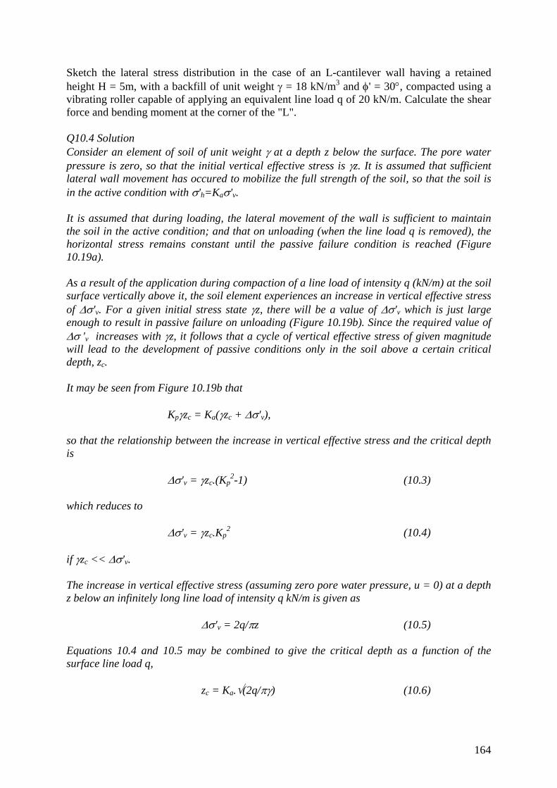
Sketch the lateral stress distribution in the case of an L-cantilever wall having a retained height H = 5m, with a backfill of unit weight γ = 18 kN/m3 and φ' = 30°, compacted using a vibrating roller capable of applying an equivalent line load q of 20 kN/m. Calculate the shear force and bending moment at the corner of the "L". Q10.4 Solution Consider an element of soil of unit weight γ at a depth z below the surface. The pore water pressure is zero, so that the initial vertical effective stress is γz. It is assumed that sufficient lateral wall movement has occured to mobilize the full strength of the soil, so that the soil is in the active condition with σ'h=Kaσ'v. It is assumed that during loading, the lateral movement of the wall is sufficient to maintain the soil in the active condition; and that on unloading (when the line load q is removed), the horizontal stress remains constant until the passive failure condition is reached (Figure 10.19a). As a result of the application during compaction of a line load of intensity q (kN/m) at the soil surface vertically above it, the soil element experiences an increase in vertical effective stress of Δσ'v. For a given initial stress state γz, there will be a value of Δσ'v which is just large enough to result in passive failure on unloading (Figure 10.19b). Since the required value of Δσ 'v increases with γz, it follows that a cycle of vertical effective stress of given magnitude will lead to the development of passive conditions only in the soil above a certain critical depth, zc. It may be seen from Figure 10.19b that Kpγzc = Ka(γzc + Δσ'v), so that the relationship between the increase in vertical effective stress and the critical depth is Δσ'v = γzc.(Kp

2-1) (10.3) which reduces to Δσ'v = γzc.Kp

2 (10.4) if γzc << Δσ'v. The increase in vertical effective stress (assuming zero pore water pressure, u = 0) at a depth z below an infinitely long line load of intensity q kN/m is given as Δσ'v = 2q/πz (10.5) Equations 10.4 and 10.5 may be combined to give the critical depth as a function of the surface line load q, zc = Ka.√(2q/πγ) (10.6)

164

Noting from Figure 10.19b that at the critical depth the residual increase in horizontal effective stress Δσ'h due to compaction is Ka.Δσ'v, and substituting for Δσ'v from Equation 10.5, with z=zc as given by Equation 10.6, we have Δσ'h at zc = √(2qγ/π) (10.7) In reality, the fill is likely to be placed and compacted in thin layers. As the initial lateral stress prior to compaction is small, Equation 10.7 gives the post-compaction horizontal stress at all depths below zc. As more and more fill is placed, however, a point will eventually be reached where the active stresses below a certain depth hc are greater than those that were induced by compaction when the layer was placed. This depth is given by the condition σ'h = √(2qγ/π) = Kaγhcor hc = (1/Ka).√(2q/πγ) (10.8) For an L-cantilever wall having a retained height H = 5 m, with a backfill of unit weight γ = 18 kN/m3 and φ' = 30°, compacted using a vibrating roller that applies an equivalent line load q of 20 kN/m, the values of zc, Δσh at zc and hc are calculated from Equations 10.6, 10.7 and 10.8 respectively as follows: Ka = (1-sin30°)÷(1+sin30°) = 0.333 zc = Ka.√(2q/πγ) = 0.333 × √{(2 × 20 kN/m) ÷ (π × 18 kN/m3)} = 0.28 m Δσ'h at zc = √(2qγ/π) = √{(2 × 20 kN/m × 18 kN/m3) ÷ π} = 15.14 kPa hc = (1/Ka).√(2q/πγ) = 3 × √{(2 × 20 kN/m) ÷ (π × 18 kN/m3) = 2.52 m At the critical depth hc, the lateral stress is 15.14 kPa (= Ka.γ.hc). The lateral stress then increases linearly to the base of the wall, where the lateral stress is Ka.γ.z = 0.333 × 18 kN/m3 × 5 m = 30 kPa. The resulting lateral stress distribution is sketched in Figure Q10.4.

165

Figure Q10.4: stress distribution for cantilever wall The shear force F at the corner of the "L" is equal to the resultant of the lateral pressure, F = {0.5 × 15.14 kPa × 0.28 m} + {15.14 kPa × 4.72 m} + {0.5 × (30 - 15.14) kPa × 2.48 m} = 2.12 kN/m + 71.46 kN/m + 18.43 kN/m ⇒ F = 92 kN/m The bending moment M is given by the sum of the forces arising from each stress block multiplied by the appropriate lever arm, M = {2.12 kN/m × 4.813 m} + {71.46 kN/m × 2.36 m} + {18.43 kN/m × 0.827 m} ⇒ M = 194 kNm/m Reinforced soil retaining walls Q10.5 A 4m-high reinforced soil retaining wall is constructed, using galvanized strip reinforcements 3.5 m long, with a cross-section of 3 mm × 80 mm. The ultimate tensile stress of the strips is 190 N/mm2, and the design must allow for an overall loss of thickness of 0.75

166

mm due to corrosion, during the anticipated working life of the structure. The strips are spaced at 1 m vertically and 0.3 m horizontally. The uppermost reinforcement is 0.5 m below the top of the wall. The surface of the backfill is horizontal. The backfill material has unit weight γ = 18 kN/m3 and friction angle φ' = 30°. The angle of friction δ between the backfill and the reinforcement is 20° (i.e. the coefficient of friction μ = tan20°.) Calculate: (a) The ultimate tensile strength of a single reinforcement strip, before corrosion. (b) The ultimate tensile strength of a single reinforcement strip, after corrosion. (c) The factor of safety FT against tensile failure (d) The factor of safety FF against pull-out. Comment on the adequacy of the design. (University of London 3rd year BEng (Civil Engineering) examination, Queen Mary and Westfield College) Q10.5 Solution (a) The ultimate tensile strength P of a single reinforcement strip, before corrosion, is given by P = ultimate tensile strength × cross sectional area = 190 (N/mm2) × (3 mm × 80 mm) = 46 500 N = 46.5 kN (b) Assume that the effects of corrosion lead to the overall loss of 0.75 mm of material from each dimension, i.e. a reduction in both width and thickness of 0.75 mm. The thickness of the reinforcing strip after corrosion is then 2.25 mm and the width 79.25 mm, giving an ultimate tensile strength P of

190 (N/mm2) × (2.25 mm × 79.25 mm) = 33 879 N = 33.9 kN

(34.2 kN if loss of width is neglected) (c) The factor of safety against tensile failure FT for a reinforcement strip at depth z may be calculated using Equation 10.13, FT = Ultimate tensile load ÷ actual tensile load, or FT = P ÷ {(Ka.γz.Δy.Δz)(1+Ka.z2/L2)} (10.13) Using the ultimate tensile strength in the corroded state, Ultimate tensile strength P = 33.88 kN Active earth pressure coefficient Ka =(1+sin30°)/(1-sin30°) = 0.333 Soil unit weight γ = 18 kN/m3

Maximum depth zmax = 4 m Horizontal spacing of reinforcement strips Δy = 0.3 m Vertical spacing of reinforcement strips Δz =1 m Reinforcement strip length L = 3.5 m

167

The actual horizontal load {(Kaγz.Δy.Δz) × (1+Kaz2/L2)} is {0.333 × 18 kN/m3 × 4 m × 0.3 m × 1 m} × {1+ [0.333× (4 m/3.5 m)2]} =10.32 kN giving FT = 33.88 kN ÷ 10.32 kN ⇒ FT =3.28 (3.31 if loss of width is neglected) (d) The horizontal load at the joint with the panel that will be required to pull the reinforcement strip out of the soil is μ×[2.bL.γz], where b is the width of the strip (= 79.25 mm in this case, allowing for corrosion) and μ is the coefficient of friction between the reinforcement and the backfill (= tan20° or 0.364 in this case). Hence the pull-out load is tan20° × 2 × 0.07925 m × 3.5 m × 18 kN/m3 × 4 m = 14.5 kN The factor of safety against pull-out is therefore FF =Horizontal load that would cause pull-out ÷ actual horizontal load, FF = 14.5 kN ÷ 10.32 kN = 1.41 The wall is closer to pull-out failure (FF = 1.41) than tensile failure (FT = 3.28) in the assumed corroded state. In this case, the value of φ' used is likely to be the critical state value, so that the calculated factor of safety against pull-out is probably reasonably reliable. The wall has a relatively wide reinforced zone, with L/H = 0.875 (where H is the overall height of the wall), so that our calculated value of FT is probably on the cautious side (see main text pages 585-588). In other words, the design is probably adequate. Note that both FT and FF are in effect partial factors of safety on strengths: FT is a factor of safety on the tensile strength of the stip material, and FF is a factor of safety on the interface friction angle, tanδ. However, in a design according to a modern code of practice such as EC7, it would also be necessary to factor the soil strength used in the calculation of the actual horizontal load {(Kaγz.Δy.Δz) × (1+Kaz2/L2)} Taking φ' = 30° and a required factor of safety on soil strength (strength mobilisation factor) Fs = 1.2 (cf BS8002), φ'design = tan-1{tan30°/1.2} = tan-1(0.481) 25.7°. This gives a factored Ka of Ka,design = (1 – sin25.7°)/(1 + sin25.7°) = 0.395 and a factored “actual” horizontal load of {0.395 × 18 kN/m3 × 4 m × 0.3 m × 1 m} × {1+ [0.395× (4 m/3.5 m)2]} =12.93 kN This gives revised values of partial safety factors on the tensile strength of the reinforcement

168

FT = 33.88 kN ÷ 12.93 kN = 2.62 and on the soil/reinforcement interface strength of FF = 14.5 kN ÷ 12.93 kN = 1.12 While the first of these is more than adequate, the second is somewhat smaller than the minimum value of 1.2 that would probably be required in design. Tunnels Q10.6 A circular tunnel, 10 m in diameter, is to be driven through a soft deposit of marine clay. The axis of the tunnel is at a depth of 20 m below the soil surface. The soft clay has unit weight γ = 16 kN/m3, and undrained shear strength τu = 40 kPa. A surcharge of q = 10 kPa acts at the surface of the clay. (a) Calculate the tunnel support pressure required just to prevent collapse, σTC If the maximum allowable surface settlement is 50 mm, estimate (b) the maximum allowable volume loss, VL(c) the load factor, LF; and (d) the required tunnel support pressure, σT Q10.6 Solution (a) The tunnel support pressure σTC required just to prevent collapse may be calculated using Equation 10.19: σTC = q + γC - 2τu.ln([2C/D]+1) (10.19) where q is the surface surcharge (= 10 kPa in this case); C is the cover or the depth of soil above the crown (20 m - 5 m = 15 m); D is the tunnel diameter (10 m); γ is the unit weight of the soil (16 kN/m3) and τu is the undrained shear strength (40 kPa). Hence σTC = 10 kPa + (16 kN/m3 × 15 m) - (2 × 40 kPa × ln4) ⇒ σTC = 139 kPa (b) The maximum allowable surface settlement Smax is 50 mm = 0.05 m. The corresponding maximum allowable volume loss VL may be calculated using Equation 10.29, Smax = 0.313.VL.D2/i (10.29) where the parameter i can be found from the empirically-derived Equation 10.30, i/z0 = 0.175 + 0.325(1-[z/z0]) (10.30) with z = 0 (i.e. at the soil surface), giving

169

i/z0 = 0.5 z0 is the depth to the centreline of the tunnel = 20 m ⇒ i = 10 m Hence, rearranging Equation 10.29, VL = Smax.i/0.313D2

VL = (0.05 m × 10 m) ÷ (0.313 × 102 m2) ⇒ VL = 0.016 = 1.6% (c) From Figure 10.32, with Smax/D = 0.05 m/10 m = 0.005, the required load factor LF is LF ≈ 0.45 (d) The tunnel support pressure σT required to give a load factor of 0.45 may be calculated using Equation 10.31 LF = [γz0+q-σT]/[γz0+q-σTC] (10.31) with LF =0.45; γz0 = 16 kN/m3 × 20 m = 320 kPa; q = 10 kPa and σTC =139 kPa. Rearranging, (330 kPa - σT) = 0.45 × (330 kPa - 139 kPa) ⇒ σT ≈ 244 kPa

170

QUESTIONS AND SOLUTIONS: CHAPTER 11 Modelling Q11.1 Compare and contrast the use of physical and numerical models as aids to design. Your answer should address issues such as the assumptions that have to be made in setting up the model, limitations as to the validity of the results, and other factors which would lead to the use of one in preference to the other. [University of London 3rd year BEng (Civil Engineering) examination, Queen Mary and Westfield College] Q11.1 Solution The answer should be in the form of a reasonably well-structured essay, illustrated with diagrams and examples as appropriate. The following notes give an indication of the expected scope. Physical models • A 1/n scale model must be tested in a centrifuge at a radial acceleration of n × g so that stresses (which govern the soil stress-strain response and possibly peak and/or undrained strength) are the same at corresponding depths in the model and the field (self-weight stress σv at depth z is ρ.g.z in the field and ρ.ng.(z/n) = ρ.g.z in the model). • A centrifuge model must be operated by remote control - in particular, it must be possible to simulate geotechnical processes such as excavation, embankment construction, diaphragm wall or pile installation, addition/removal of props etc. • Must look carefully at scaling relationships and real-time effects of the simulated events (e.g. are they essentially drained or undrained?) • Models are often plane strain, but 3-D modelling is not difficult. Numerical models • Often need to run in 2-D (plane strain or axisymmetric) because full 3-D modelling would require excessive CPU time. • Plane strain modelling can be difficult to interpret, e.g. for rows of piles. (Physical modelling would enable this problem to be represented more reasonably by a line of discrete piles, even if deformation overall were constrained to be in plane strain). • Results of an analysis can be critically dependent on the soil model and parameters used. Soil behaviour is still very difficult to describe mathematically. Problems can also arise in the use/omission of interface elements e.g. between soils and structures. • It can be easier to follow construction processes in detail than in a physical model. General • Before using the results from either technique directly in a design, the applicability of the simplifying assumptions made in setting up the model would have to be considered very carefully. • Physical modelling is useful to identify mechanisms of collapse and deformation, and to calibrate numerical models. • Both can be used for parametric studies, to develop an understanding of the relative influence of different effect, and for investigating the sensitivity of the response of a system to unknown or uncertain boundary conditions or parameters in design.

171

In situ testing Q11.2 (a) Describe the principal features of the Menard and self-boring pressuremeters, and compare their advantages and limitations. (b) Figure 11.27 shows a graph of corrected cavity pressure p as a function of the cavity strain εc for a self-boring pressuremeter test. The test was carried out in a borehole at a depth of 11

m in a stratum of sandy soil of unit weight 20 kN/m3. The piezometric level was 1 m below the ground surface. Estimate (i) the in situ horizontal total stress, (ii) the coefficient of earth pressure at rest, Ko, and (ii) the soil shear modulus, G; Q11.2 Solution (i) The in situ lateral total stress σho is given by the lift-off pressure at which the cavity starts to expand. From the graph (Figure 11.27), σho ≈ 165 kPa (ii) At the test depth of 11m, the vertical total stress σv is 11 m × 20 kN/m3 = 220 kPa. The pore water pressure (assuming hydrostatic conditions below the piezometric surface) u is 10 m × 10 kN/m3 = 100 kPa. Thus the vertical effective stress σ’v = σv - u = 120 kPa; the horizontal effective stress σ’h = σh - u = 65 kPa, and Ko = σ’h/σ’v =65/120 ⇒ Ko = 0.54 (iii) The shear modulus G is obtained from the slope of the unload/reload cycle using Equation 11.24: G = 0.5 × (ρ/ρo) × (dp/dεc) (11.24) where ρ is the current cavity radius and ρo is the cavity radius at the start of the test (i.e. at εc = 0). The average cavity strain over the unload-reload cycle shown on Figure 11.27 is about 1.5%, i.e. ρ/ρo = 1.015 (≈ 1). From the graph, the slope of the unload/reload cycle dp/dεc ≈ 500 kPa/1.1% = 45.5 MPa. Hence G = 0.5 × (ρ/ρo) × (dp/dεc) = 0.5 × 1.015 × 45.5 MPa ⇒ G ≈ 23 MPa Ground improvement Q11.3 Write brief notes on: (a) Grouting (b) Surface compaction and heavy tamping

172

(c) Cement and lime stabilization In each case, your answer should include (but not be restricted to) a discussion of the ground conditions and soil types for which the method is suitable. [University of London 3rd year BEng (Civil Engineering) examination, Queen Mary and Westfield College] Q11.3 Solution (a) Grouting • Purpose: water stop (physical cut-off) or mechanical improvement (strength/stiffness) by bonding particles. Usually works by penetrating voids in between particles. Coarser soils are easier to permeate than finer soils owing to larger voids. • Materials: cement based grouts are ok for fissured rocks and coarse materials (gravels). Cement particles will not penetrate a soil finer than a very coarse sand. Chemical/silicate grouts must therefore be used for medium/coarse sands. For finer soils, acrylic resin solution grouts are needed. It is, however, possible to inject grout into fissures and slip surface in clay soils to stabilize (at least temporarily) embankments and slopes. • If the grout will not penetrate into the voids or pre-existing fissures, it can cause hydrofracture. Empirically, fracture pressure is ~ 2 to 6 × overburden. Long thin fractures are not helpful, but short wedge-shaped fractures can be useful in compacting the soil. Need to use pastes to achieve this. • Generally, water stopping is easier than ground improvement, because it is necessary only to permeate the coarser zones. For satisfactory ground improvement all particles must be bonded, but a strong grout is not always necessary. • Parameters governing the effectiveness of a grouting operation include the grout viscosity, shear resistance (shear stress as a function of strain rate), pumping pressure and flowrate into the ground: all must be carefully controlled. Viscosity varies with gel strength, and rate of gelation (setting) will depend in turn on factors including the ground temperature. • Other applications include jacking up buildings, underpinning and compensation grouting (which is pre-emptive and used to prevent settlements of the ground surface due to e.g. tunnelling). (b) Surface compaction and heavy tamping • Surface compaction is most effective when applied to granular materials placed in layers. It involves the application of shear stresses (e.g. using smooth, tyred or sheepsfoot rollers); dynamic energy (e.g. using pounders or rammers); or vibration; or a combination of these. • The objective is to densify the soil, increasing its (peak) strength and (more especially) its stiffness. • Soils must be compacted in thin layers, generally 0.3 m to 0.5 m thick. • The technique is not suitable for clays, except perhaps clay fills in clods in order to reduce the volume of air voids between the clods. In this case, there is a need to re-mould the clods by applying shear stresses: vibratory energy is ineffective. • Compaction of any material - particularly a clay - requires careful monitoring and control. • Heavy tamping involves dropping a large mass (up to 170 tonnes) from a height of up to 22 m in order to compact the soil. Usually, the mass is dropped onto a number of points in a grid or triangular pattern.

173

• The aim is to treat the soil at depth (up to 40 m: empirically, D (m) ~ 0.5 × √(WH) where W is the mass in tonnes and H is the height of drop in m), rather than just thin layers as in surface compaction. • Originally intended for granular (free-draining materials), it can be effective in low-permeability soils because it causes fractures in the upper layers which allow water to escape in response to the excess pore water pressures generated by dropping the weight. Also, air voids can be compacted quite readily. The timing of the drops requires some thought in these materials. • It is necessary to spread a 1 - 2 m thick stone blanket on the surface, to support the plant and prevent cratering. (c) Cement and lime stabilization • Both methods work by chemically bonding the soil particles. Typically, 2 - 10% cement or lime is added. • Cement stabilization works with all soils (except perhaps coarse gravels where the voids are too large, and some inorganic soils). Cement and water react to form cementitious calcium silicate and aluminium hydrates which bond the soil particles together. This is the primary reaction, which releases Ca(OH)2 (slaked lime) which may then react with the soil (especially clay minerals) to give a further beneficial effect. • Lime stabilization essentially works on the basis of the secondary reaction with cement, and requires a substantial proportion (>35%) of fine particles (<60μm). The reaction initially involves the exchange of cations (e.g. sodium for calcium) between the lime and the clay, which causes the clay to coagulate. • In the second stage of the clay/lime reaction, silica is removed from the clay lattice to form products similar to those resulting from the hydration of cement. This is the main source of “improvement”, and the effectiveness of the cementation increases with particle surface area. • Both processes improve volume stability, stiffness and unconfined compressive strength. Cement stabilization depends on adequate mixing and compaction, which can be difficult to achieve with clay soils. • The addition of lime to clay improves workability because the plasticity index is decreased, although the exact mechanism of this (in terms of changes to wLL and wPL) will depend on the activity and mineralogy of the clay. • The degree of cementation increases with the quantity of lime added, but the lime reaction uses the silica naturally present in the soil. There is therefore no point in adding more lime than will use up the available silica - indeed, adding further lime beyond this point can be counterproductive. Q11.4 Give an account of: (a) The principal applications of grouting in geotechnical engineering (b) The factors influencing the penetration of grouts into soils (c) The major differences in properties and performance between cement-based grouts and low viscosity chemical grouts [University of London 3rd year BEng (Civil Engineering) examination, Queen Mary and Westfield College] Q11.4 Solution The answer should be in the form of a reasonably well-structured essay, illustrated with diagrams and examples as appropriate. The following notes give an indication of the expected scope.

174

(a) Principal applications of grouting in geotechnical engineering • Prevention of groundwater flow (formation of a physical cut-off) - by blocking the soil pores • Increasing soil stiffness and strength - by bonding soil particles • Jacking up buildings • Underpinning • Compensation grouting (used to prevent settlements of the ground surface due to e.g. tunnelling) • Stabilization of geotechnical structures such as tunnels, excavations and slopes (b) Factors influencing the penetration of grouts into soils • Particle/void size of the soil • Viscosity and gel strength of the grout • Pressure at which the grout is pumped (c) Major differences in properties and performance between cement-based grouts and low viscosity chemical grouts • Cement based grouts consist of fine cement particles in suspension, and the pore size that these grouts can penetrate is limited by the size of the cement particles. Cement grouts will penetrate into fissures and voids in coarse soils (i.e. gravels), but will not penetrate a soil finer than a very coarse sand. Grouts containing smaller particles such as sodium silicate in colloidal suspension are used for medium/coarse sands. For fine sands and silts, an acrylic resin solution grout must be used. • Lower viscosity grouts are also better able to penetrate soils at a given pumping pressure, because the energy lost in overcoming the shear stresses that resist flow is reduced.

175

SOLUTIONS MANUAL -...

Documents

Transcript of SOLUTIONS MANUAL -...