TICAM REPORT 95-09June 1995

Solution of Exterior Acoustic Problems by theBoundary Element Method at High Wave Number,

Error Estimation and Parallel Computation

P. Geng, J.T. Oden, & L. Demkowicz

Solution of Exterior Acoustic Problems bythe Boundary Element Method at HighWave Numbers, Error Estimation and

Parallel Computation

P. Geng, J. T. Oden, and L. Demkowicz

Texas Institute for Computational and Applied Mathematicsthe University of Texas at Austin

Abstract

This paper is concerned with the application of the boundary ele-ment method to the exterior acoustical problem at high wave numbers.The major issues here are to establish a strong theoretical foundationfor the application of the Burton-Miller integral equation and developa practical way for its numerical implementation.

Unlike many conventional_approaches, the problem in this studyis formulated by the Galerkin method. Through an analysis on its el-lipticity, the Burton-Miller equation is proven to be well-posed in theHl/2-Sobolev space and its approximation can attain a quasi-optimalconvergence rate. The Galerkin scheme avoids sensitive propertiesof hypersingular integration, simplifies the numerical implementation,and improves the quality of the numerical solutions, especially in therange of high wave numbers. An L2-norm residual error estimationtechnique is also implemented for an adaptive scheme for these prob-lems.

The numerical implementation is completed on parallel distributed-memory machines. The validation of the method for high wave num-bers is done through tests on a series of numerical examples.

1

1 IntroductionMuch of the structural acoustics is concerned with the classical problem ofinteraction of the motion of a solid structure with that of a fluid into whichthe structure is immersed. Small perturbations in the velocity or pressurefields of the fluid create waves that impinge upon the structure and sC<i:tterinto the fluid-structure domain while small motions of the structure may ra-diate energy into the surrounding fluid media. A major issue involved in thestudy is the propagation of waves in the fluid media. In classical models, thefluid is treated as a quiescent, inviscid medium capable of transmitting acous-tical wave in a uniform pressure field that is characterized by the Helmholtzequation defined on an unbounded exterior domain.

A classical technique for handling the exterior problem characterizing thefluid is to convert the exterior differential Helmholtz equation into an integralequation. Then a discretization of the integral equation by the boundaryelement method (BEM) allows one to confine the numerical approximationsto the fluid-structure boundary-the so-called wet surface. Consequently, thedimensionality of the problems is reduced by one and the exterior boundaryissues are avoided.

Unfortunately, the integral form of the Helmholtz equation is not per-fectly equivalent to the original differential form of Helmholtz equation onthe exterior domain and, thus, at certain frequencies, the so-called forbiddenfrequencies, the integral operator involved in the integral equation becomessingular and the solution of the integral equation is not unique. Severalboundary integral formulations have been proposed t-? overco:r;nethis non-uniqueness problem; see (2, 11, 22, 24, 26, 27], and the CHIEF ( CombinedHelmholtz Integral Equation Formulation ) method, proposed by Schenck(24], is a widely used method in engineering computation. In the CHIEFmethod, the system of linear equations is combined with a few additionalequations generated from the Helmholtz integral equation with the sourcepoints in the interior of the closed boundary. The method can be used toanalyze a class of acoustical scattering problems, but because the stabilityof the method depends strongly on the number and locations of the sourcepoints chosen in the computation, the method may not be reliable and effi-cient at high wave numbers.

A method which seems to be valid for all cases was proposed by Burtonand Miller in 1971 [2]. However, direct implementation of the ~urton-Miller

2

integral formulation using the conventional collocation scheme leads to theproblem of so-called hypersingular integrals and the method itself is verycomplicated and often yields very poor results.

Unlike the conventional approach, the numerical implementation in thisstudy is based on the Galerkin scheme. The Galerkin method for the bound-ary integrals has been treated extensively by Wendland and Hsiao [9,28].They proved that a large class of integral equations are strongly elliptic typefor which the Galerkin method shows an optimal convergence rate. In thispaper, we will prove that the Burton-Miller formulation defines a stronglyelliptic equation in a proper Hilbert space so that an optimal convergencerate is expected for the numerical solutions; furthermore, the hypersingularintegrals involved in the original formulation can be avoided by performinga special transformation on the Galerkin weak form.

Although the details of an adaptive method are not presented in thiswork, it is worth to mention that the boundary element procedures describedhave been developed in a special hp-hierarchical data structure proposed in[5, 6]. This data structure allows the mesh size and order of polynomialinterpolation to be varied over the mesh during computation. In addition,an a posteriori error estimate originally proposed in [5] is further developedin this study. The error estimation is based on the L2-norm of the residualwhich is simple to calculate and yields good results in experiments. All ofthese features provide a good basis for the development of adaptive methods.

The paper is organized as follows. We first describe the mathematicalmodel for the problem of interest and give a careful analysis on its math-ematical foundation together with an a posteriori error estimation scheme;next we discuss some basic principles in the problem discretization; and fi-nally, experimental results are presented.

2 Problem StatementThe problem under consideration is the exterior acoustical scattering prob-lem. To be precise, we wish to find the pressure distribution p = p(x) in adomain ne exterior to a closed bounded surface r. The scalar field p satisfiesthe exterior Helmholtz equation

(1)

3

and the boundary condi tions

(2)

_ (3)

where k = w j c is the acoustic wavenumber with c and w, the speed andangular frequency of sound, p = Ixl represents the distance between originand the position x, n denotes the outward normal unit vector on the surfacer, pS = p - pine is the scattered wave pressure, and pine is the pressureof incident wave. The boundary condition (3) is the Sommerfeld radiationcondition and in (2), G and g are two given functions on the boundary r.

The problem defined above can be converted into an integral eq1lation onthe boundary r, i.e.,

1 r oiI>(kr) Op(y) inc2"p(x) - Jr[p(y) on(v) - on(y) iI>(kr)] dS(y) = p (X), (4)

In (4), x and yare two points on the boundary, l' = Iy - xl and n(·) denotesthe outward normal unit vector at the corresponding position, iI> representsthe fundamental solution of the Helmholtz equation and is of the form

in two dimensions

in three dimensions

andiI>( kr) = exp( ikr)

47rr

where HJ is the Hankel function of the first kind of zero order and i = v=I.Applying the directional derivative ojon(x) to both sides of (4) leads toanother form of the Helmholtz integral equation:

~ op(x) _ 0 r (p(y) oiI>(kr) _ op(y) iI>(kr) ] ds(y) = opine(x) (5)2 on(x) on(x) Jre on(y) on(y) on(x)

We refer here to (4) as the normal Helmholtz integral equation and (5) as thehypersingular integral equation.

4

In 1970, Burton and Miller [2] proved that neither (4) nor (5) but theircomplex linear combination is equivalent to the original differential equation.Using (2), the Burton-Miller formulation can be written as

1 r o<I>(kr)2" (1 + aG(x)] p(x) - Jr ( !Lf __\ - G(y)iI>(kr)] p(y)dS(y)

o r oiI>(kr)-a ~ , , Jr [ !Lf __\ - G(y)iI>(kr)] p(y)dS(y) = J(x)

where a is a complex constant whose imaginary part cannot be zero and

J(x) = pine(x) + 19(y)iI>(kr)dS(y)

(6)

Equation (6) defines the mathematical model used in this investigation tosolve the problem of the acoustic wave scattering on the exterior domain r!e.

3 Strongly Elliptic Equations and Their Ap-proximation

The theoretical foundation of the model problem defined in (6) can be es-tablished through the theory- of strongly elliptic equations. We here give asummary on the work given in (12, 28, 18] and discuss certain mathematicalprinciples underlying strongly elliptic problems. An analysis on the ellipticityof the Burton-Miller equation will be provided in the next section.

For generality, we consider here a linear equation (differential equation orintegral equation) on some given domain !1, i.e.,

Au=J (7)

subjecting to appropriate boundary conditions where A: VCr!) --t V'(r!) is alinear operator on a Hilbert space V = VCr!) of functions defined on nandV' is its dual space. The operator A is said to be strongly elliptic if it canbe expressed as the sum

A=D+C

5

(8)

where D maps V continuously onto V' and is strongly coercive in the sensethat there exists a {3 > 0 such that

(Dv, v) 2: {3 II v II~, Vv E V (9)

and C is a compact operator on V, where II . Ilv represents the norm on thecorresponding V space, and (.,.) denotes duality-pairing on V' x V. Notethat if D = I is an identity operator, the operator A = I + C is called aFredholm operator of the second kind.

Let us define the bilinear or sesquilinear forms corresponding to A by

a(u,v) = (Au,v)

and the linear form corresponding to f in (7) by

lev) = (J, v).

Then (7) is equivalent to the following variational problem:

Find u E V such that

a(u,v) = lev) VvE V (10)

For the approximation of (10), let {vn} be a sequence of approximatingfinite dimensional subspaces of V which satisfies the following density as-sumption:

(D) For any v E V there exists a sequence Vi E V su~h that vi E Vi and

.lim Ilv - villv = O.1-+00

(11)

Then, for a given subspace vn c V, the Galerkin approximation of (10) canbe written as

Find uh E vn such that

(12)

The following properties of the strongly elliptic equation

(D + C)u = fare known (12]:

6

(13)

• as mentioned, the operator D : V -7 V' in (13) is continuous andcoercive; therefore, according to the Lax-Milgram theorem (see(20, p31)), the inverse mapping D-1 : V' -7 V exists and is continuous.Applying D-1 to both sides of (13) leads tQ the equation

(I + D-1C)u = F. -(14)

where I : V -7 V is the identity mapping and F = D-1 f. Here, D-1 isa continuous mapping from V'to V and C is a compact mapping fromV to V'. It follows that the product D-1C : V -7 V is compact andhence (14) defines a Fredholm equation of the second kind.

• according to the Fredholm alternative (see [15, pAl)), the equation(13) is uniquely solvable only if the operator 1+ D-1 C is injective; i.e.,existence of a solution follows its uniqueness.

• we observe that (13) and (14) are in fact equivalent to each other, andthat existence of a solution to (13) follows if uniqueness (injectivity)can be proven.

For the stability and convergence of Galerkin approximations, the follow-ing theorem is found in [28].

Theorem 3.1 Let A be a strongly elliptic operator on a Hilbert space V andlet (1) or (l0) be uniquely solvable. Then there exists an N > 0 such that(l2) is uniquely solvable for all vn with n ~ N, and there also hold astability condition

IIUhllv::; clilullv,and an a priori error estimate

(15)

(16)

where u is the solution of (1) or (lO), uh is the corresponding approximatesolution, and cl and C2 are positive constants independent of u, uh, and n.

7

4 EllipticityIn this section, we prove that the Burton-Miller formulation characterizes astrongly elliptic equation on the space of Hl/2(r). As a special case of theSobolev fractional space HS(r) ( s E lll, s ~ 0), Hl/2(f) is defined as thecompletion of COO(f) in the norm of

2 2 r r lu(x) - u(y)12II U 111/2 = II u 110 + Jr Jr 1__ __1~-Ll f? dS(y) dS(x)

where m represents the dimensionality of the surface f ( m = 1 for theproblem in two-dimensions and m = 2 for the problem in three-dimensions), and

II u II~= t u2(x) dS(x).

is the L2-norm on f. The space Hl/2(f) is also a Hilbert space and its dualspace IS

(Hl/2(f))' = H-l/2(f).

Mathematically, the space Hl/2(r) is related to the space of functions of finiteenergy interior to the surface f by the trace theorem: for smooth enough f,there exists a constant c > 0 such that

lI,u Ih/2 < c II u IIHl(O)

where II . IIHl(O) denotes the HI-norm on the interior domain r!, and ,u isthe trace of u on f. For more details, see Adams [1].

Returning to (6), we rewrite it in the form

Find p E H} (f) such that

1 ) T-(1 + aG Ip - MkP + LkGp - a(NkP - Mk Gp) = f (17)2

Here, I is the identity operator and Lk, Mk, M[ and Nk are linear operatorsdefined as follows:

• the single layer potential

LkV(X) = t ~(kr)v(y)dS(y),

8

(18)

• the double layer potential

r oiI>(kr)MkV(X) = Jr ~LL\ v(y)dS(y),

• the adjoint of the double layer potential

M[ vex) = on~x) 1r iI>(kr)v(y)dS(y),

• and the hypersingular operator

Nkv(x) = ~ r oiI>(h)on(x) ir cL f __ \ v(y)dS(y)

(19)

(20)

(21)

The following results are given by Costabel in [3]:

Lemma 4.1 On a Lipschitz boundary, the operat01's:

1 Ht+U(r)Lk : H-2+U(r) -t

Mk : Ht+U(r) -t Ht+u (r)

MT. H-t+U(r) 1 ~ (22)k . -t H-2+U(r)

Ht+U(r) 1Nk: -t H-2+~r)

are well defined and continuous for all (J E (-1/2, 1/2].

and

Lemma 4.2 There exists a compact operator T : Ht(r) -t H-t(r) and apositive number). such that

Re((Nk - T)v, v) ~ ). II v III2

1where II . III represents the H2 -norm.

2

9

1Vv E H2(r)

From Lemma 4.1, we can conclude that Lk and Ah are continuous map-pings from Ht(r) to Ht(r) and M[ is a continuous mappings from Ht(r)to HO(f). For simplicity, we only consider the problem in which G given in(2) is a smooth function on the boundary r; then (1+a G)I is at least a con-tinuous mapping form Ht(r) to Ht(f). Because the imbedding: Ht ~ HSis compact if t > s, Lk, Mk, M'[, and (1 + aG) 1 define compact mappIngs

1 1from H2(r) to H-2(r). Let

D = -a(Nk - T)

and1

C= -(l+G)1 - A1k + GLk - a(T - G!III'[).2

Then (6) can be written as

(D+C)p=f

According to Lemma 4.2, D is a strongly coercive operator. Moreover, eachoperator involved in C is the compact operator on Ht(r) and so is C. Then,the main result in this section is

Theorem 4.1 The equation (6) defines a stTOngly elliptic equation on Ht (r),Thus, the problem is well posed if it contains at most one solution.

The uniqueness of the solution of (6) for the Neumann boundary condi-tion was proven by Burton and Miller in [2] and the proof for the Dirichletboundary condition is similar. However, for the more general condition givenin (2), the original Helmholtz equation en as well as the boundary integralequation may not be uniquely solvable at certain wavenumbers or frequencieswhich are usually refered to as the resonant frequencies or natural frequen-cies. In summary, we have the following conclusion for this section

Theorem 4.2 At non-resonant frequencies or wavenumbers, the boundaryintegral equation (6) is uniquely solvable; and there exists an N > 0 suchthat for n ~ N, its Galerkin approximate solution pn is stable and con vergeswith an optimal rate, i. e.

II p -lliv :S c inf II p - vh II!vhEVn 2

where p is the exact solution, c is a constant independent of p, ph and n, andII . II! represents the norm on Hl/2(f).

2

10

5 The Variational Formulation and Descriti-zations

A special problem arising in the implementation of Burton-Miller formulationis that the integral

o r oiI>(kr)Jr ~::LL \ p(y )ds(y)

in (6) cannot be evaluated easily in a meaningful way.customary to write (23) in the form

(23)

Symbolically, it is

(24)t ~_~f~~~~~:__\ds(y).

The integral kernel o2iI>(kr)/on(x)on(y) contains hypersingular term and itis easily verified that as r -7 0 in two dimensions

o2iI>(kr) 1on(x)on(y) = O(r2)'

and in three dimensions

Although the hypersingular integrals can be computed numerically in thesense of the finite part integral ( see [5, 16] for details ), the implementationfor such procedures is complicated and the accuracy is often very poor.

The method used in this study to avoid hypersingular integral kernelsassociated with (24) was proposed in [7, 14]. The method requires that theproblem be formulated in a weak (Galerkin) approach and is completed intwo steps. The first step, proposed by Burton and Miller (2], is based on animportant identity derived by Maue [17] and Mitzner (19]:

t p(y) ~_~f~~~~~L\ds(y) =

i{(n(y) x \7yp(y) ] . (n(x) x \7xiI>(kr) ]

+ k2 n(x) . n(y) iI>(kr) p(y) } ds(y).

11

(25)

In the second step, multiplying both sides of (25) by a test function q(x)( the conjugate of q(x) ), and integrating the whole equation again over r,yields

r - r 02iI>(kr)Jr

q(x) JrP(Y) ~Lf __\~ __f__\ds(y)ds(x) =

1q(x) 1{[n(y) X \7yp(y) ] . [n(x) X \7xiI>(kr) ]

+ e n(x) . n(y)iI>(h)p(y) } ds(y) ds(x) (26)

It is easy to verify ( see [7, 14] for deta.ils ) that for the piecewise smooth testfunction q and trial function p,

1q(x) 1[ n(y) X \7y p(y) ] . [ n(x) x \7xiI>(kr) ]ds(y) ds(x) =

-11iI>(kr)[ n(y) x \7yp(y)], [n(x) X \7xq(x)] ds(y) ds(x),

then, (26) can be written as

r - r 02iI>(kr)Jr q(x) JrP(Y) !:l __ f __\~_f __\ds(y)ds(x) =

11 iI>(kr) { - [n(y) x \7yp(y) ] . [n(x) X \7xq(x) ]

+ e n(x) . n(y) q(x) p(y) } ds(y) ds(x). (27)

In two dimensions, (27) reduces to

r - r 02 iI>(kr )irq(x) JrP(Y) on(x)onfH\ds(y)ds(x) =

r r oq(x) op(y)JrJr iI>(kr)(- or (x) or(y) + k2n(x). n(y)q(x)p(y)] ds(y)ds(x) (28)

where rex) and r(y) are the positive tangential directions at x and y.

12

Multiplying both sides of (6) by q(x), integrating the whole equationover r and replacing the corresponding terms by (27) or (28), we obtain thefollowing two- and three-dimensional versions of the variational formulationof (6):

Find p E H t (r) such that in two dimensions,

~1[1+ aG(x) ] p(x) q(x) ds(x)

r r 0iI>(kr)- Jr Jr[ on(x) - G(y)iI>(kr) ] p(y) q(x) ds(y) ds(x)

r r op(y) oq(x) 2 oiI>(kr)-a Jr Jr { -iI>(kr) or(y) or(x) + [ k r(x) . r(y)iI>(h) - ~__fu\ G(y) ]

p(y) q(x) } ds(y) ds(x) = 1f(x) q(x) ds(x),

and in three dimensions,

~ r [ 1+ aG(x) ] p(x) q(x) ds(x)2 Jr .

-ll( 0':l~\~~) - G(y)iI>(kr)] p(y) q(x) ds(y) ds(x)

-a 11r{ -iI>(kr) [n(y) x \7yp(y)]. [n(x) X \7xq(~)]

0iI>(kr)+ (k2 n(x), n(y)iI>(kr) - ~__f __\ G(y)] p(y)q(x) } ds(y) ds(x)

=1f(x) q(x) ds(x)

(29)

(30)

1for any q E H'i(r).Equations (29) and (30) contain only the weak singular and regular inte-

grals which can be treated easily in numerical implementations. Approxima-tion of p and q in (29) or (30) by the linear combinations of th~ s<l..~ebasis

13

functions:

p(x)N

Lpi 17i(X)i=l

(31 )

Nq(X) = L qi 17i(X)

i=l

leads to a system of linear equations for pi (i = 1, ... , N), i.e.,

(32)

or

N

Lali pi = bl,i=l

Ap =b

1= 1,..,N (33)

(34)where A = {ali}NXN is a non-symmetric, complex and dense matrix andb = {bl}NXl are complex vectors. Solving (33) or (34) gives the approximatepressure solution vector p on the boundary f.

6 A Posteriori Error EstimationIn this section, we discuss the theoretical foundation of a posteriori errorestimation and its application to the problem (29) and (30).

6.1 Theoretical foundationThe method of a posteriori error estimation developed here is based on fun-damental properties of Fredholm equation of the second kind and of Galerkinapproximations. The problem of seeking a solution of the Fredholm equationin L2(f!) is stated formally as follows:

Find p E L2(n) such that

(I+C)p=! (35)

where I is an identity operator, C is a compact operator on L2(n) and!E L2(f!).

Let Vh c L2(f!) be a finite dimensional space, and instead of n, let hbe a parameter such that whenever h -t 0, we mean that the dimension of- --

14

yh ---t 00. Let ph be an approximate solution from yh and the correspondingerror eh be defined as

eh = p _ ph. (36)

Let Ih : L2(f!) ---t yh to be the orthogonal projection onto the subspace yl>,i.e, for any p E L2(f!),

We have the following classical result for the compact operator C andL2-projection l1h:

Lemma 6.1 Suppose that operator C: L2(f!) ---t L2(f!) is compact. Thenthere holds

lim II C(I - l1h) 11= 0h-O

where II . II represents the norm on the space £(L2(f!), L2(f!))

Proof: See [25].

(37)

•Another classical result for the L2-projection l1h and the Fredholm equation(35) is given in the next lemma.

Lemma 6.2 Assume (35) is uniquely solvable; then for the compact operatorC and the L2-projection l1h, the inverse operators (I + Cl1ht1 exist andare uniformly bounded for all sufficiently small h, i.e., there exist positivenumbers ho and At such that, for all h S ho,

(38)

Proof: See (15].

•Lemmas 6.1 and 6.2 can further lead to the following result:

Lemma 6.3 Suppose that (35) is uniquely solvable, then there holds

II Ceh 110= µ(h) II eh 110

andlimµ(h) = 0h_O

15

(39)

(40)

where eh is the error defined in (36), ph is a Galerkin approximate solutionfrom a finite dimensional space Vh c L2(n), and II . 110 represents the L2_

norm.

Proof: We first define Uh as

(41)

Let Ih : L2(f!) ---t L2(f!) be the orthogonal L2-projection onto Vh. TheGalerkin approximate solution ph satisfies the equation

which means thatIIh(I + C)ph = IIhf

or

and then from (41)IIhph = IIhUh· (42)

Applying IIh to both sides of (36), and substituting it into (42) leads to

Iheh = IIh(p - ph) = IIh(p - Uh) (43)

and, from the definition of Uh,

Ceh = C(p - ph) = f - p - C ph = -(p - Uh)

Therefore,

(44)

p - Uh + CIIh(p - Uh)

-Ceh + CIIh(p - Uh)

-Ceh + CIIheh

-C(I - IIh)eh. (45)

Replacing p - Uh with -Ceh on the left hand-side of (45) leads to the relation

(I + CIIh)C eh = C(I - IlJ,) eh

16

or

II Ceh II~ µ(h) II eh IIwhere

µ(h) =11 (I + CIhtl 1111 C(I - Ilh) II .From Lemma 6.1 and Lemma 6.2,

lim II C(I - Ilh) /1= 0h-.O

and II (I + CIlhtl II is uniformly bounded by (38). Thus we finally have(40) and complete the proof.

•For any approximate solution ph, we define the corresponding residual of

the Fredholm equation (35) as

f h C hrh =. - p - p

or

Moreover, from (39),

/I rh 110=/1 eh + Ceh 110= (1 + µ(h)) II eh 110,

l.e.(1 - Iµ(h)l) II e

h 110 ~ II rh 110 ~ (1 + Iµ(h)l) II eh 110

and, from Lemma 6.1, we have

lim µ(h) = 0h-.O

(46)

(47)

Therefore, we have the following theorem on the asymptotic behavior ofII rh 110:

Theorem 6.1 Suppose that the Fredholm equation(35) is uniquely solvable.Then there holds

. II rh 110 - 111m -h-.O II eh 110

(48)

For the boundary integral equation, II rh 110 is readily computable after solv-ing Ph; thus Theorem 6.1 in fact suggests that II rh 110 can be used as an aposteriori error estimate.

17

6.2 Applications

In this subsection, we consider the application of the error estimation to thetwo kinds of boundary integral formulations, the normal Helmholtz integralformulation and the Burton-Miller integral formulation.

For convenience, we rewrite the normal Helmholtz integral formulation(4) in the operator form

(49)

where11 = pine + 1r g(y )<P( kr )dS(y)

The operator Nh - LkG is a compact operator in U(r), which occurs if bothLkG and !11k are compact operators; then the U-norm of the residual canbe used as an error estimator for (37). Recalling Lemma 4.1, on a Lipschitzboundary r, the single layer potential Lk can be a continuous operator fromL2(r) to Hl(r) which indicates Lk is a compact operator from L2(r) to L2(r).As noted earlier, G is considered to be the smooth function in this study,and so the operator LkG is a compact operator in L2(r). For the doublelayer potential Mk, Lemma 4.1 only states that it is a continuous operatorfrom L2(r) to L2(r) on a Lipschitz boundary r ( taking (J" = 0 for Mk in(22) ). However, if the boundary r is smooth enough ( r E C2+{3((3 > 0) ),the kernel ( oiI>(kr)/on ) of double layer potential Mk in fact is continuouson r (see (4, p 300)); thus Mk is also a compact operator in. L2(r) and so isMk - LkG. Then, the L2-norm of residual

(50)

can be used to estimate the L2-norm of the real error II eh 110 = II p - ph 110where p represents the exact solution.

For the Burton-Miller formulation, its solution belongs to the space ofHt(r) and, according to Hsiao [10], the residual rh must be computedthrough the hypersingular integral formulation (5), i.e.,

18

where8pine r oiI>( kr) 1

h = a;;: + Jrg(y) 811,(V) dS(y) - 2"g,

and then(51)

where Cl and c2 are two positive constants, ph is the approximate solutionof the Burton-Miller formulation, and II . 11_1and II . 111represent the H-L

2 2

norm and HLnorm, respectively. Because H-Lnorm is not easily com-putable in practice, II rh 11_1cannot be directly used as an error estimation.

2

A simple approach used in this study is that technically, we can substitutethe approximate solution of the Burton-Miller formulation into Eq.(50) toobtain a residual fh and then use L2-norm of 1~h, i.e., II fh 110, as an errorestimation of II eh 110. Numerical experiments consistently suggest that

r Whllo = 1.h~ Ilehllo

7 Numerical Experiments

The experiments reported here focus on the performance of the method athigh wavenumbers, the effectivity of a posteriori error estimation, and theapplication of the method to transient acoustical problems. The tests areperformed on conventional sequential machines as well as parallel distributed-memory machines. The details of the parallel implementation and its per-formance can be found in (8].

7.1 Two test problems

In general, the solution of exterior acoustic scattering problems with theboundary condition of

op = Gpon

can be expressed in form of

19

on r (52)

(53)

where G is the function given in (2) and pine and pS represent the incidentand scattering wave pressures, respectively. According to (13], for the planeincident wave

pine = Pine exp( ik p cos 8) = Pine exp( ikx) (54)

impinging on a cylinder ( in two dimensions) or a sphere ( in three dimensions), and G = c being a constant ( see Fig. 1 ), the scattered pressure pS canbe evaluated by the series

in two dimensions

in three dimensions(55)

where a is the radius of the cylinder or sphere. In (55), Hm and hm representthe Hankel function and spherical Hankel function of the first kind of orderm, respectively, Pm are Legendre polynomials, and as noted earlier, k is thewave number. In two dimensions, the coefficients Bm are given by

!!! kJ:r,(ka) - cJm(ka)Bm = -Pinebm( -1) 2 kH:n(ka) _ cHm(ka)

where Jm is the Bessel function of the first kind of order m, and

bo = 1 and bm = 2 (m = 1,2,3, ... );

and in three dimensions, the coefficients Bm are computed through

(56)

(57)

(58)

where jm is the spherical Bessel function of the first kind of order m. The spe-cial functions, Hm, hm, Jm and jm are computed using the routines providedin [23].

The second test problem is designed to test the method on the problemswith non-smooth boundary (corners or edges). For the Neumann boundarycondition

opan

20

m = 1, .. · (59)

it easily verifies that the pressure solution of the corresponding radiationproblem

IS

1(2" 1+ Mk + a Nk) P = (~ + Lk + aM[) oH:n(kr)eikB

on (60)

(61)

where Hm is still the Hankel function of the first kind of order m, and Mk,

Nk, Lk and MI are operators defined in (18)-(21). For simplicity, we use theproblem containing only one corner (see Fig. 2).

7.2 Applicability of the method for problems withhigh wave numbers

In this experiment, the performance of the boundary element method forsolving problems with high wave numbers is explored. Two indices involvedare the L2-norm of the relative error II eh 110and the L2-norm of the relativeresidual II ;.h 110which are computed through the formulae:

and

II eh II~= I['(ph - Pe)(ph - Pe) ds(r)I[' PePe ds(r)

II ;. II~= Ir rhrh ds(r)

I[' PePe ds(r) .

(62)

(63) -

where Pe and ph represent the exact solution and numerical solution, respec-tively, and rh is the residual computed by (50).

Example 1: Comparison of the Burton-Miller integral equation and thenormal Helmholtz integral equation.

The 2D acoustic scattering test problem defined in (52) - (58) is solvedusing two different formulations: the Burton-Miller formulation and the nor-mal Helmholtz integral equations, through a range of wave numbers. Thefollowing input data are chosen for the test problem:

c = 1 and 0, a = 1 and Pine = 1.

21

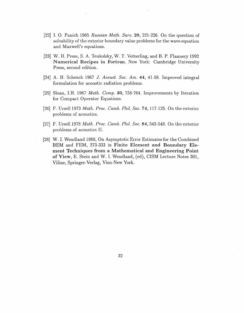
Figures. 3 and 4 show results obtained by using the normal Helmholtz in-tegral equation and the Burton-Miller formulation for a uniform mesh of 64quadratic elements with £ = 1. In both cases, the problem was solved for arange of wave numbers from 10 to 50 with 6.ka = 0.1.

Two figures indicate that the error increases as the wave number increases.Fig. 3 clearly indicates that the normal Helmholtz integral equation is ..un-able to provide stable solutions at high wave numbers and while solutions(Fig. 4) of Burton-Miller formulation are stable throughout entire range ofwave numbers tested. Figures 3 and 4 also indicate that the L2 residual errorestimates produce satisfactory results. For example, as shown in Fig.4, theestimated error is almost equal to true error when ka < 30 and through therange of ka = 30 to 50 , the maximum difference between true error andestimated error is less than 20 percent. The result for the case of £ = 0 (i.e. dpjdn = 0, rigid scattering) are similar and are, therefore, not presented.

Example 2 The relationship between kh and the L2-1'elative error.In Theorem 3.1, we indicated that the approximation solution ph of the

integral equations will converge at the rate of

where II . "v is the norm corresponding to the space Y where the problem isdefined. For simplicity, we here consider only the error in L2-norm. In (64)

is the best possible interpolation error in the space of yh; and if Pe is smoothenough, we have

where p~m+1) represents m + 1 derivatives of the exact solution Pe and m isthe approximate order of local elements. For harmonic vibrating problems,we assume that the exact solution Pe is oscillating in the sense that

22

Then, if c is a constant in (64), the solution error will depend only on kh,I.e.,

(65)

1

BecauseCf

k = - = 27fAw

and

h =number of elements per unit length

where Cf represents the sound speed in the fluid medium and A is the wavelength, kh is a measure of the number of elements per wave length, and (65)in fact states a. well known rule of thumb in engineering computation, i.e.,the solution error depends on the the number of elements per wave length.

However, Theorem 3.1 states only that c is independent of p, ph and h; itmay still depend on k. If c increases as the wave number k increases, the ruleof thumb can not be applied and this will deteriorate the efficiency of themethod in the range of high frequencies. Because the conclusive theoreticalanalysis on the influence of k on c is not available at present, we shall test itexperimentally.

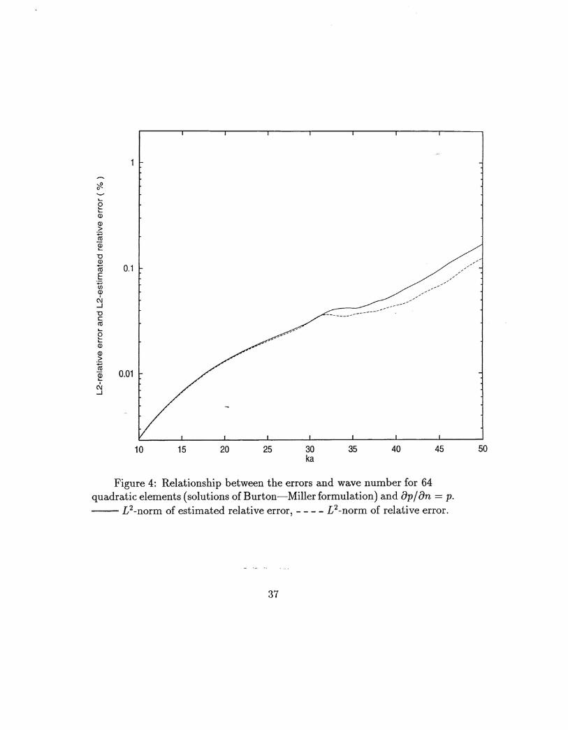
Figures 5 and 6 shows the computed rela.tionship between L2-norm rel-ative error" eh 110 and kh for two- and three-dimensional problems, respec-tively. The experiments were also performed on the scattering test problemsas in the previous example, and the following input data are given

£ = 0, a = 1 and Pine = 1

with different kh.In two dimensions, Fig. 5 shows that the relative error" eh 110 will depend

only on kh if kh is not too large (kh :S; 2.5). In three dimensions, weonly test the case of kh = 1.79, and the results indicate that the L2-norm ofrelative error is less than 5% if we control kh to be less than 1.79.

7.3 The Effectiviness of the A Posteriori Error Esti-mation

A comparison of the L2-norm of the error and the L2-norm of the residualis further studied in this experiment. The effectiviness of the L2-residual

23

estimate is measured by an effectivity index defined by

ir .. . d II rh 110euectIvlty III ex = II eh 110 (66)

Equation (66) gives a global measure of the effectiviness of the errorestimation. However, the efficiency of adaptive methods is determined bythe local quality of the error estimate: the effectivity of error estimationon each individual element. The local effectivity of the error estimation ismeasured by

local effectivity index = II rh

IIi

where /I . /Ii represents the L2-norm on the element i.Theoretically, we can only prove the global result,

r II rh

110- 1h~" eh 110 -

(67)

(68)

when rh and eh are the residual and error corresponding the approximatesolution of the normal Helmholtz integral equation on a smooth boundary r.As noted earlier, we here use h as a parameter such that whenever h ---7 0,either the mesh size (real h) approaches to 0 or the approximate order oneach local element approaches approaches to 00. However, the major goalhere is to establish an error estimate for the Burton-Miller formulation on aboundary which may possess only piecewise smoothness. Thus, we test theeffectiveness of " rh /10 as an error estimator when the residual rh is calcu-lated based on the approximate solution of the Burton-Miller formulation ona smooth or piecewise smooth boundary.

Example 3 The effectiviness of the error estimationFor k = 15, a = 1 and £ = 1, the 2D acoustical scattering test problem

defined in (52) - (58) is solved by the Burton-Miller formulation with differentmesh sizes h and approximate orders m. The corresponding effectivity indicesare summarized in Fig. 7. The results verify (68) which states that as thedegrees of freedom increasing ( h ---7 0 or m ---7 00), the L2-norm of residualwill approaches the L2-norm of true error.

24

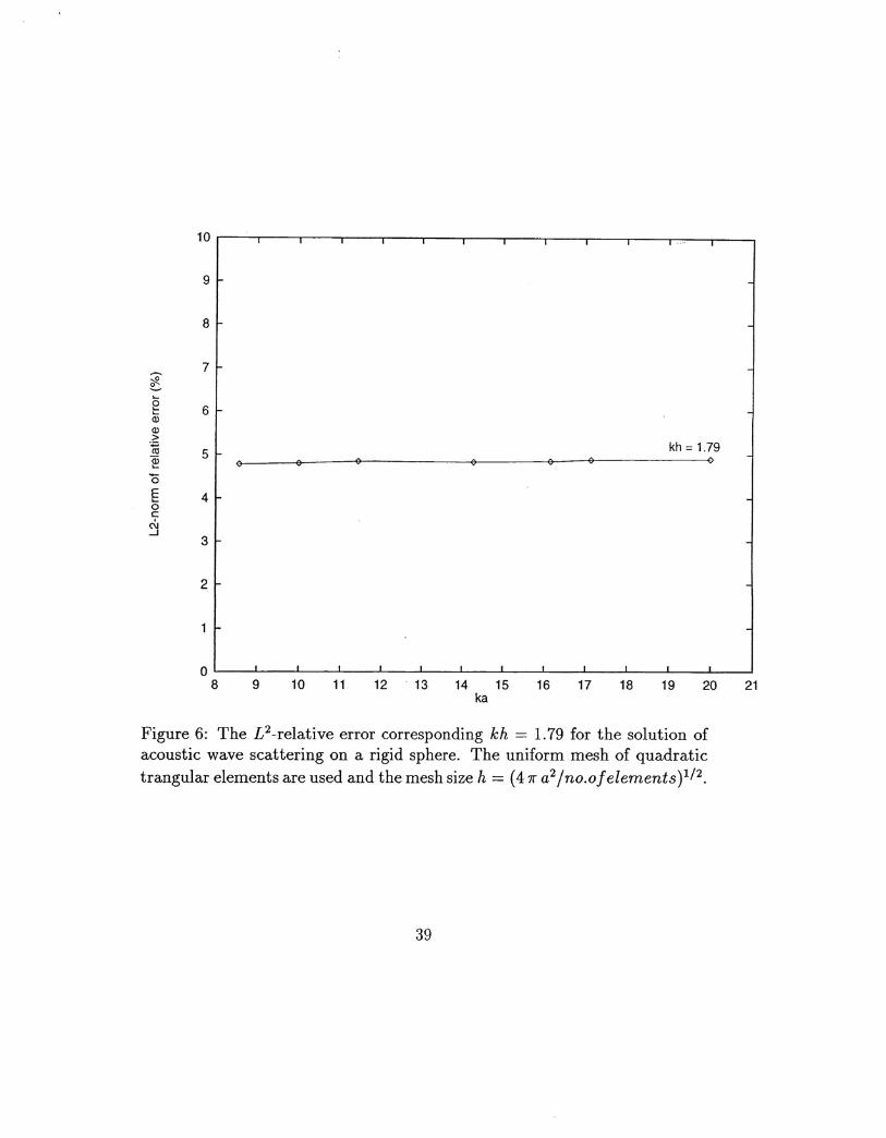
Furthermore, we give some results at very high numbers ( k = 400 intwo dimensions and k = 20 in three dimensions). Figures 8 and 10 comparethe numerical solutions and corresponding exact solutions for the two- andthree-dimensional problems. In both cases, the L2-norm relative error andL2-norm estimated error are very close to each other ( 2.28 % and 3.34 % inFig. 8; and 4.9 % and 5.2 % in Fig. 10 ). Figures 9 and 11 further comparethe local error II eh Iii and II rh Iii where II eh Iii and II rh Iii are computed,respectively, by

and

for any given element ri. In Fig. 9, the estimated error is almost equal tothe true error. For the three-dimensional test problem (Fig. 11), the errorestimator clearly locates the elements with big errors. All of these shows thatour error estimation is accurate and efficient.

Example 4: A further survey of the effectivity of error estimation on theproblem with non-smooth boundary

In the preceding section, we stated that the double layer potential op-erator Mk E £(L2(r),L2(r)) is only proven to be compact on a smoothboundary r, thus, theoretically the error estimation proposed in this studyis valid only for the problems with a smooth boundary. In this experiment,we conduct some tests to evaluate the effectiviness of the error estimationfor the problems with piecewise smooth boundaries.

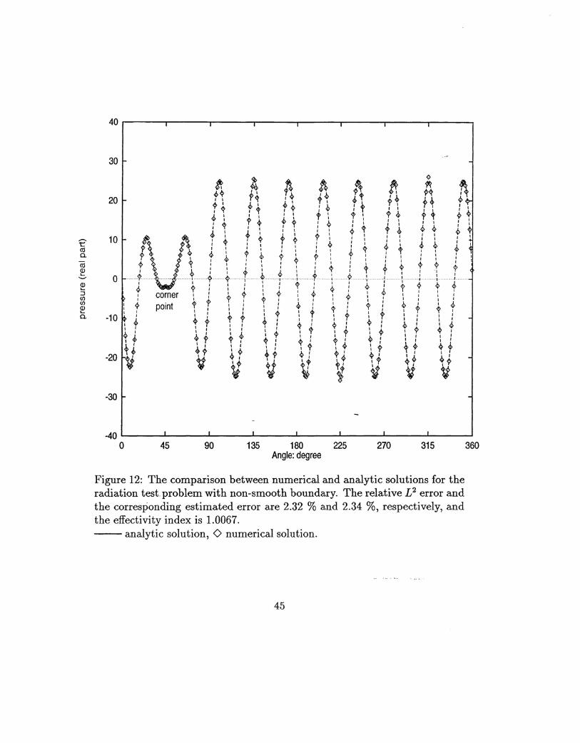
The experiment is conducted on the radiation test problem defined in(59)-(61) with the boundary shape as shown in Fig. 2. A uniform meshof 32 quadratic elements is used and m = 10 and k = 5 are chosen. Thecorner point in Fig. 2 coincides with the node shared by the element 4 and 5.Figure 12 shows the comparison between the numerical solution and analyticsolution and the global effectivity index. In this case, the global effectivityindex is 1.0067 being very close to 1. Table 1 lists the local effectivity indiceson each element. Except in the element 4, the local effectivity indices hereare all very close to 1. The local effectivity index for the element 4 is about0.89 which is a little lower than the average effectivity indices for the rest of

25

elements and this means that the corner node may have some local influenceon the effectiviness of the error estimation.

7.4 The application of the method to transient acous-tical problems

Theoretically, the linear acoustical problems can be solved by two differentapproaches: in the time domain or in the frequency domain. The transientacoustical problem in time domain can be transformed into a static acousti-cal problem in frequency domain through the Fourier transformation, thenthe solution of the original transient problem can be obtained by the inverseFourier transformation on solutions of static problems on different frequen-CIes.

A major advantage of solving the exterior scattering problem in the fre-quency domain is that the static acoustic problem on the exterior domaincan usually be converted into an integral equation on the interior boundary,so that the dimensionality can be reduced by one and the infinite boundarycondition is satisfied automatically. Furthermore, in practice, the number offrequencies which needs to be considered in the frequency domain methodis often much less than the number of time steps taken in the time domainmethod as the response to higher frequency is critically damped and insignif-icant.

In this experiment, we test the possiblity of solving transient acousticproblem in the frequency domain by the boundary element method. Thefollowing aco.ustic incident pulse is chosen

{

-I + 32(r + 0.25)2 - 256(r + 0.25)4 - 0.5 S; r S; 0pine(r) = 1- 32(r - 0.25? + 256(r - 0.25)4 0 < r S; 0.5

o 0.5 < Irl S; T(69)

to compute 2D wave scattering problem as shown in Fig. 13 with the radiusof cylinder a = 0.5. Here r = x - ct and the time unit is lief. The incidentwave pulse must be supposed as a periodical function, and the period Theremust be large enough so that the solution at the interested time period isnot affected by the solution wave from other periods. In this example, we areinterested in the solution in the time period 0 S; t S; 2 and T = 5.2, i.e.,-5.2 S; t S; 5.2, is selected. Then, t.he.incid~nt wave in (69) is decomposed

26

into the sum of a series of sine functions, i.e.,

N i7rTpine( T) = I.:Pi sineT)

i=l

and N = 2,048. At most frequencies, the amplitude Pi is in fact alqlOstzero, we here only solve the problem at a frequency when its correspondingamplitude satisfies

Pi > 0.01 max (pj).1<!,j<!,N

(70)

Then, instead of 2,048 different frequencies, we only need to solve the prob-lem for 124 different frequencies with the maximum wave number about 45.

In each frequency, the pressure distribution on the boundary r was solvedby the boundary element method; and then, its contribution at the point x onthe exterior domain ( Ixl > 0.5 ) is computed through the exterior boundaryintegral equation

The uniform mesh of 128 quadratic elements on the boundary are used in theexperiment. Figure 13 presents the results ( the acoustic pressure contours)at t = 0 and t = 2/cf and in the region of -2 :::;x :::; 2 and 0 :::; y :::; 1.9.The result shown in Fig. 13 is almost exactly match the results obtained bythe time domain method prosposed in [21] but with much less computationalcost.

8 Summary and Future WorkThe major difference between the approach used in this work and conven-tional approaches is that the approximation in the boundary element methodis based on Galerkin approximation of the Burton- Miller hypersingular inte-gral formulation of the exterior Helmholtz equation. The advantages of usingGalerkin approximation demonstrated in this study are listed as follows

• To overcome the problem of non-uniqueness at forbidden frequencies,the formulation proposed by Burton and Miller in [2] is used. A spe-cial difficulty that arises in applying their method is the occurrence of

27

hypersingular integrals in the boundary integral equation. However,if the Galerkin method is used to approximate the weak form of thisequation, the resulting formulation contains only regular and weaklysingular integrals. Implementation of the new formulation is straight-forward and produces stable solutions even at very high wave numbers.

• For strongly elliptic problems, the Galerkin scheme has a well estab-lished theoretical foundation. After proving herein that the problemsinvolved in this study are of strongly elliptic type, it follows that theGalerkin approximations are quasi-optimal, i.e, for any approximatesoltltion uh on a finite dimensional space Vh, there holds

• Using certain fundamental properties of Galerkin methods and Fred-holm integral equations of the second kind, we prove that the L2-normof the residual of the normal Helmholtz integral equation approa.chesL2-norm of error asymptotically, i.e.,

lim II rh

110 = 1h-+O,p-+oo II eh 110

Because II rh 11o is computable after solving the boundary elementproblem, it can be used as an a posteriori error estimation. Numericalexperiments further suggest that the error estimation II rh 11o can pro-vide a very accurate estimation for the global error as well as the localerror.

As is well known, a major problem in the application of the boundaryelement methods is that the system of linear equations generated by thismethod is full and non-symmetric and has to be solved by a direct denselinear solver. Consequently, the O( n3) cost of dense solvers, in combinationwith the O(n2) memory required to store a matrix of dimension n limitsthe size of problem that can be solved using this method. Furthermore,because of the involvement of singular integrals, the formation of the linearsystem in the boundary element model is often much more expensive thanthe formulation of linear systems when other numerical techniques are used.

28

These facts have limited the range of sizes of problems to which the boundaryelement method can be applied.

However, the range for which boundary element methods can be usedcan be greatly expanded through the utilization of massively parallel super-computers. Dense linear solvers lend themselves particularly well to parallelcomputing, achieving very good efficiency even when very large numbers ofprocessors are used. The parallel computation can also significantly reducethe computational time in the formation of the linear system.

The parallel implementation, including the formation of linear system,linear dense solver, and error estimation has been initially done in [8]. Fu-ture work will concentrate on improvement in the efficiency of the currentparallel algorithms and on methods to increase capacity, Advances in theseareas should help to make this particular type of boundary element methodan efficient tool for solving large-scale and high-frequency acoustical prob-lems.

Acknowledgement: The support of the Office of Naval Research of thiswork under Contract N00014-89-J-3109 is gratefully acknowledged.

29

References[1] R. A. Adams 1975, Sobolev Space. New York, Academic Press.

[2] A. J. Burton and G. F. Miller 1971 Proc, Roy. Soc. London Ser. A323,201-210. The application of integral equation methods to the numericalsolution of some exterior boundary-value problems.

(3] M. Costabel1988 J. Math. Anal. 19, 613-626. Boundary Integral Oper-ators on Lipschitz Domains.

(4] R. Courant and D. Hilbert 1962 Methods of Mathematical Physics,Vol. II, New York: Interscience.

[5] 1. Demkowicz, J.T. Oden, M. Ainsworth and P. Geng 1991 Journalof Computational and Applied Mathematics 36, 29-63. Solution of elas-tic scattering problems in linear acoustics using h-p boundary elementmethods.

[6] L. Demkowicz, J.T. Oden, W. Rachowicz, and O. Hardy, 1989, CompoMeth. in Appl. Mech. and Engrg. 77, 79-112. Toward a Universal h-pAdaptive Finite Element Strategy Part 1: Constrained Approximationand Data Structure.

[7] 1. Demkowicz, A. Karafiat and J.T. Oden 1992 Compo Meths. Appl.Mech. Engrg. 101, 251-282. Solution of elastic scattering problems inlinear acoustics using_h-p boundary element method.

[8] P. Geng, J. T. Oden and R. A. van de Geijn 1995. Massively ParallelComputation for Acoustical Scattering Problems using Boundary Ele-ment Methods. To appear in Journal of Sound and Vibration.

(9] G. C. Hsiao and W. 1. Wendland, Tech. Report No. 101-A, AppliedMathematics Institute, University of Delaware. Super-approximation forboundary integral methods.

(10] G. C. Hsiao, R. E. Kleinman, R-X Li, and P. M. van den Berg 1990,Residual Error-A Simple and Sufferent Estimate of Actual Error in So-lutions of Boundary Integral Equations, 73-83 in Computational En-gineering with Bound~ry EleI1lents Vol. 1: Fluid and Potential

30

Problem, S. Grilli, C. A. Brebbia, and A. H-D Cheng (ed). Boston:Computational Mechanics Publications.

[11] D. S. Jones 1989 Q. J. Mech. Appl. Math. 44, 129-142 Integral equationsfor exterior acoustic problem.

[12] C. Johnson, and J. C. Nedelec 1980 Math. Comp., 35 1063-1079. On theCoupling of Boundary Integral and Finite Element Methods.

[13] M. C. Junger and D. Feit 1972 Sound, structures, and their inter-action. Cambridge, Massachusetts: The MIT Press.

[14] A. Karafiat, J.T. aden and P. Geng 1993 International Journal ofEngineering Sciences 31, 649-672. Variational formulations and hp-boundary element approximation of hypersingular integral equations forHelmholtz-exterior boundary-value problems in two dimensions ..

[15] R. Kress 1989 Linear Integral Equations, Applied Mathematical Sci-ences 82, Springer-Verlag.

[16] H. R. Kutt 1975 Report WISJ( 179. On the numerical evaluation of finitepart integrals involving an algebraic singularity. Pretoria: The NationalResearch Institute for Mathematical Sciences.

(17] A. W. Maue 1949 Z. Phys. 126, 601-618. Zur Formulierung Eines Allegmeinen Beugungsproblems Durch Eine Integralgleichung.

[18] S. G. Mikhlin 1965 The Problem of the Minimum of a QuadraticFunctional. San Fransisco: Holden Day Inc ..

(19] K. M. Mitzner 1952 J. lvlath. Phys. 7, 2053-2060. Acoustic Scatteringfrom an Interface between Media of Greatly Different Density.

[20] J. T. aden and G. F. Carey 1983 Finite Elements, MathenaticalAspects, Prentice-Hall, Inc., Englewood Cliffs, New Jersey.

[21] J. T. aden, A. Safjan, P. Geng, and 1. Demkowicz 1994, Multi-Level,hp-Adaptive, Time Domain Methods for Large-Scale Structural Acous-tics Simulation, in Large-Scale Structure in Acoustics and Elec-tromagnetics, National Academy of Science (to appear).

31

(22] I. O. Panich 1965 Russian Math. Surv. 20, 221-226. On the question ofsolvability of the exterior boundary value problems for the wave equationand Maxwell's equations.

[23] W. H. Press, S. A. Teukolsky, W. T. Vetterling, and B. P. Flannery 1992Numerical Recipes in Fortran. New York: Cambridge UniversityPress, second edition.

[24] A. H. Schenck 1967 J. Acoust. Soc. Am. 44, 41-58. Improved integralformulation for acoustic radiation problems.

[25] Sloan, I.H. 1967 Math. Compo 30, 758-764. Improvements by Iterationfor Compact Operator Equations.

[26] F. Ursell1973 Math. Proc. Camb. PhiZ-Soc. 74, 117-125. On the exteriorproblems of acoustics.

[27] F. Ursell1978 A1ath. PTOC.Camb. Phil. Soc. 84,545-548. On the exteriorproblems of acoustics II.

[28] W. I. Wendland 1988, On Asymptotic Error Estimates for the CombinedBEM and FEM, 273-333 in Finite Element and Boundary Ele-ment Techniques from a Mathematical and Engineering Pointof View, E. Stein and W. I. Wendland, (ed), CISM Lecture Notes 301,Viline, Springer-Verlag, Vien-New York.

32

Table 1: The comparison of local L2-norm errors and L2-norm residuals forthe radiation test problem with non-smooth boundary.

Element No. Local Effectivity Index Element No. Local Effectivity Index1 0.983 17 1.0132 1.028 18 1.0083 1.039 19 1.0084 0.890 20 1.0095 1.061 21 1.0126 1.011 22 1.0067 1.021 23 1.0108 0.979 24 1.0109 1.056 25 1.01010 1.006 26 1.00911 1.013 27 1.00812 1.005 28 1.00713 1.012 29 1.01114 1.007 30 1.01215 1.011 31 1.00616 1.006 32 1.045

33

y

Incident wave

incident wave

•y

1\X

x( a, 0, 0 )

Figure 1: Acoustic scattering test problems in two- and three-dimensions.

34

yCorner point

x

Figure 2: The radiation test problem.

35

rfl.L-

oL-L-

a>a>>:;::;ella>L-

ua>iiiE~a>N-lUCellL-oL-L-

a>a>>~<iiL-I

C\/-l

0.1

0.01

10 15 20 25 30ka

35 40 45 50

Figure 3: Relationship between the errors and wave number for 64quadratic elements (solutions of normal Helmholtz integral equation).- L2-norm of estimated relative error, - - - - L2-norm of relative error.

36

"!-....a........(I)

(I)

>§(I)....u(I)

.... 01E .(jj(I)

N...JUCIII....a........(I)

(I)

>~~ 0.01I

(\J...J

10 15 20 25 30ka

35 40 45 50

Figure 4: Relationship between the errors and wave number for 64quadratic elements (solutions of Burton-Miller formulation) and op/ on = p.- L2-norm of estimated relative error, - - - - L2-norm of relative error.

37

10

_ kh=4

8

6

4

/

//"

/"

/"

//

/"

//

//

//

//

ii

ii

kh=3"5

kh=3

2________________________________________________--- ----n_ - -- ----- -- --- -- ---- -- - - kh=2.5

- ~~

oo 50 100 150 200 250

ka300 350 400 450 500

Figure 5: The relationship between kh and L2-relative error for the solution ofacoustic wave scattering on a rigid cylinder. The uniform mesh of quadraticelements are used and the mesh size h = 27ra/no. of elements.

38

10

9

8

~7

~g 6Q)

Q)>~

5 ~kh = 1.79

~ <:> a a a a a 0

13E 40cN-I

3

2

o8 9 10 11 12 13 14 15

ka16 17 18 19 20 21

Figure 6: The L2-relative error corresponding kh = 1.79 for the solution ofacoustic wave scattering on a rigid sphere. The uniform mesh of quadratictrangular elements are used and the mesh size h = (47fa2/no.ofelements)1/2.

39

XQl"0C

2

1.8

1.6

1.4

1.2

0.8

0.6

0.4

0.2

o10 50

Log N (N: degrees of freedom)150 200 250

Figure 7: The effectivity indices of the error estimation for different meshsize h and element order p. The 2D acoustic scattering test problem is solvedby the Burton-Miller formulation with k = 15, a = 1 and c = 1

40

2.5

2

1.5

t?ella.ro

0.5~---c0

S 0.0·C

en"0Q) -0.5...:J(/)(/)Q)...a. -1

-1.5

-2

-2.50 pi/4 pi/2 3pi/4 pi

Figure 8: The comparison between numerical and exact solutions around thecylindrical boundary with k = 400, a = 1 and c = 1. Because of symmetry,only the solution from 00 to 1800 around the cylindrical boundary is plotted.The relative L2 error and the corresponding estimated error are 2.28 % and2.35 %, respectively. The problem is solved with a uniform mesh of 1,024quadratic elements and 2,048 degrees of freedom. The problem is solved inan Intel ipsc/860 parallel machine by using 16 processors.- analytic solution, - - - - numerical solution.

41

0.0055

0.005

0.0045

0.004"iii::J

~ 0.0035~"0c 0.00311l.....0..........~ 0.0025aE.....0 0.002cN...J

0.0015

0.001

0.0005

01 64 128 192 256 320 384 448 512

element number

Figure 9: The comparison between the local error and the estimated localerror correponding to Fig. 8. Because of symmetry, only results on theelements from 1 to 512 are presented.o estimated local error, - - - - true local error.

42

2 I I I I I

1.5

tcoa.«i 0.5Q)....~c0:s.0 a I-u'C]?"0

-0.5 ~<IJ....::J(f)(f)Q)....a.

-1

-15 ~ \

-2-pi

I

-pi/2

.. ~ d> .. c .

a

..'n"k 'H~I''I"'!' nf·· ,¢> ..

..L

pi/2

. -

pi

Figure 10: The comparison between numerical and analytic solutions aroundthe curve of ";x2 + y2 = 1.5a, z = 0 for the test problem in three dimensionswith k = 20, a = 1 and £ = 1. The relative L2 error and the correspondingestimated error are 4.9 % and 5.2 %, respectively. The problem is solvedwith the mesh of 1,568 quadratic elements and 3,138 degrees of freedom inan Intel ipsc/860 parallel machine by using 32 processors.- analytic solution, 0 numerical solution.

43

0.016 I I T

0.014 o o oo

o

196

o

o

I

168

""""'()""""I'

"""":l>"",I -,o,,,,l>'".I,4I>,,.~,

{fR""II

o"""i~,,I,,,,{>,,,"Q,,,,bIii~,,<tI>I

~ /.0', v,~,&Q111 I-, ,, ,

:;1:~,

o

140

"""""'()" -;,,,,,

1>,,","<},,,,l>lit",,~: ,I ,

lL!c"]OQ ~

l>¢i'00,:1. :-, ,, ,,- ,-, ,

1·'-iJ

",

"""":?,.,,,,~,," ,,"

<t,,,~,,',",,<t,,I

0'0i!}o~$

{>,,0 ,, I,.0 ,III I, ,, ,"I I,-=,,'

,-,II,IIo :, ,, ,, ,, ,'·0 () ,% ~"() ,

l> 0 :, ,'f! I~I{> :, ,

Iii rl~,f-:'d

,,,,,l>,," ,,,(),,,,,,l>

""""""l()"

84 112element number

,,,,,,,,l>,,"

"<}

"""""":l>

I

56

:1>,-,IIII,,,I

o

...L

28

0.01

o1

0.012

0.004

0.002

0.006

0.008

co:J

:Q(/)

~"0CcoL.-g(])

"0EL.-acN-l

Figure 11: The comparison between the local error and the estimated localerror correponding to Fig. 10 ( Only results on the elements from 1 to 196are presented ). 0 estimated local error, - - - - true local error.

44

40

30

Q)L-

:J(f)(f)Q)L-a.

20

10

o

-10

-20

-30

<>

~ ~ ~ A ~ ~ ~ ~tt f~ ,~ +~ ~t it it t~.~' ~, ~~ ,~ If " " , ~,~ ,t I, ,1" ~, ~~ tt {l,1 I I I 1.' T I I I I I I I I"', t~ "'t '9 I' " Q~ '~:~ " I, I, ~t t~ 1,9,

~~ ~t 1'~: '::: II:&, ~ 'A.'~ r~ '9 I' A' Q~ 1~ I Y I 1 I I 1 'f' I I Q)tt t ., " " " ~~ ,t I , '~~!~ Q t ~ ~ ~ l t: , : I : 1 l :

r t """" y , , I I ~ 4> y y ~

t Q ~ t ! : i i J \ f t ~ ~ .:nnn:nnni nnn: nnn:nnr nnlnnninnn:nnt nnnt nnnrnnn: nnTn~.nnn:n nn~ nnnn:. nnnrnn :. + t t +). ~ "'", 'A ,). 4>, '4>""<t' Y , I ~ I Y I '+' I 9 1 I I I , I

I corner : ' ~ , ~ I , I : , ~ I 9' 'Q, ·t t t , I I I ~ I ~ 'T: ,t t '~ pOin " ',' 'A. I <b ,J, ',~ " ':I I I I Y ITT T I I I

' l' tt ~I" 1,~'~, 'QQ vt " 'I~.I. v, '1. ,t~,I I I I I I 'A.. I Tit I Y " I I1· l' '4> 'y " J" 9' " ,)...~ "'t t I ~, ~' T A " 1~ ~<l>I I I I " t: I ~ , ..... I t "f It'+~ ~t ~t tt t: tJ t+ ~~ ~~~ ~ V V ~ V ~ ~ V

-40o 45 90 135 180 225

Angle: degree270 315 360

Figure 12: The comparison between numerical and analytic solutions for theradiation test problem with non-smooth boundary. The relative L2 error andthe corresponding estimated error are 2.32 % and 2.34 %, respectively, andthe effectivity index is 1.0067.- analytic solution, 0 numerical solution.

45

1.5

1.0

0.5

0.0-2

1.5

1.0

0.5

0.0-2

-1

-1

a

t=Ol/cf

a

t = 11/Cj

1

2

2

Pressure

10.846154

0.6923080.5384620.384615

0.230769

0.0769231-0.076923-0.230769-0.384615-0.538462

-0.692308

-0.846154-1

Pressure

0.913846

0.770959

0.628072

0.4851860.342299

0.1994120.0565253

-0.0863614-0.229248

-0.372135

-0.515022

-0.657908

-0.800795

-0.943682-1.08657

Figure 13: The pressure solution of the transient acoustical problem by theboundary element method at t = 0 and t = 2 l/ef.

46