Solow-Swan growth model and the fortunes of the commons

Kumar Aniket

University College London

15 September 2019

Abstract. In the traditional Solow model, output saved in a period is transformed into new

private capital through the saving channel after depreciation. Consequently, the traditional

Solow growth framework has only one kind of capital, i.e., one that is funded through private

savings and hence privately owned. There is no role for an alternative channel through which

output is taxed and then transformed into public goods (infrastructure) after accounting

for depreciation. Barro (1990) models this alternative channel but assumes that it only

funds pure public goods that don’t depreciate over time. The pure public goods assumption

effectively suppresses the dynamics of this alternative channel and ensures that it collapses

into the saving channel. We explicitly model this alternative channel and assume that it

transforms taxes into congestible public goods, which depreciate over time and call it the

fiscal channel. We find that the fiscal channel interacts with the traditional saving channel

in an counter-intuitive way. This is because the fiscal and saving channels create different

kind of capitals through distinct processes and these capitals then impact each others’

marginal productivity of capital. We show that a country can only get prosperous if both the

proportion of output transformed into private capital through savings and the proportion

of output transformed into congestible public goods through taxation is sufficiently high.

Keywords: Economic Growth, Public Goods, Infrastructure Finance, Congestion

JEL Classification: O11, O16, O41, O43

E-mail address: k.aniket@ucl.ac.uk .

Date: 15 September 2019.

1

“An enormous influence on the fate of nations emanates from the economic

bleeding which the needs of the state necessitates, and from the use to which

the results are put.”

Schumpeter et al. (1918)

1. Introduction

Why does newly installed infrastructure in developing countries often wither away over

time? Why have empirical studies never been able to find a strong impact of foreign aid

on long-term economic growth or per-capita income? What kind of reforms will turn a

low-income country into a middle-income country? These are the stark questions that still

confound policymakers and academics.

The Solow-Swan growth framework1 remains the most tractable model for understanding

economic growth in countries where the evolution of technology is not an endogenously

determined process. Its intellectual influence is hard to overstate given its pedagogical value,

its relevance in contemporary policy-making and its use in a range of disciplines beyond

economics. Yet, the Solow-Swan framework is unable to shed any light on the questions

posed above. The objective of the paper is to augment the Solow-Swan growth framework

to answer these questions. At the heart of the Solow-Swan growth framework lies the notion

that output that is not consumed can be costlessly transformed into new capital that can then

be used to produce output in the next period. Exactly what Solow-Swan framework means

by its physics-defying notion of capital is important to understand if it is to be augmented

to answer the questions we pose.

This paper contends that the received wisdom on Solow-Swan growth framework2 over

the years has stuck too closely to the original formulation. The rather broad category of

privately owned capital is unable to satisfactorily accommodate tax-funded publicly owned

1The Solow-Swan model of economic growth was developed independently by Robert Solow and Trevor Swanand published simultaneously in Solow (1956) and Swan (1956).2This paper uses the word framework to refer to the way the have been received, which maybe distinct fromthe ideas in the original papers. There is some evidence in Solow (2007) and La Grandville and Solow (2009)that this is an important distinction.

2

Output today

PrivateSavings

ConsumedOutput Non-consumed

Output

Output tomorrow

PrivateCapital

Saving Channel Fiscal Channel

PublicCapital

Tax collectedby government

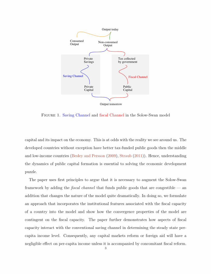
Figure 1. Saving Channel and fiscal Channel in the Solow-Swan model

capital and its impact on the economy. This is at odds with the reality we see around us. The

developed countries without exception have better tax-funded public goods then the middle

and low-income countries (Besley and Persson (2009), Straub (2011)). Hence, understanding

the dynamics of public capital formation is essential to solving the economic development

puzzle.

The paper uses first principles to argue that it is necessary to augment the Solow-Swan

framework by adding the fiscal channel that funds public goods that are congestible — an

addition that changes the nature of the model quite dramatically. In doing so, we formulate

an approach that incorporates the institutional features associated with the fiscal capacity

of a country into the model and show how the convergence properties of the model are

contingent on the fiscal capacity. The paper further demonstrates how aspects of fiscal

capacity interact with the conventional saving channel in determining the steady state per-

capita income level. Consequently, any capital markets reform or foreign aid will have a

negligible effect on per-capita income unless it is accompanied by concomitant fiscal reform.3

At the heart of Solow-Swan framework is the saving channel through which capital accu-

mulation channel takes place and results in the growth of per-capita income. This channel

costlessly transforms output that is not consumed into new capital stock. The new capital

stock can then either augment capital stock of the economy or compensate for the deprecia-

tion of the pre-existing capital stock. Capital stock accumulates or de-accumulates until the

economy reaches a steady-state where the output that is saved and transformed into capital

just about meets the depreciation needs of the pre-existing capital stock and the capital

accumulation process comes to a standstill. There are of course specific conditions under

which one or more steady states exist and the economy converges or diverges from these

steady states.

The Solow-Swan framework was able to show that the economy converges to a unique

steady state if the production function of the economy exhibits constant returns to scale and

diminishing returns to capital. These properties of the production function and competitive

markets for factor inputs create the tendency of convergence and homogenisation within

the functional sub-units of the modern economy. Given this tendency to homogenise, the

distinction between production process at the aggregate level and within its functional sub-

unit is inconsequential. Herein lies at least one justification for categorising all variety of

capital under the rubric of just one homogenous type of capital.

The received wisdom on Solow-Swam framework suggests that output and capital variables

do not represent their actual physicality but an abstract notion of resources. These resources

are then represented by nominal assets that can be traded in the capital markets. The

homogenisation tendency in the modern economy helps in unifying the myriad physicality of

capital and output into one single asset class.3 Hence, the critical role played by the saving

channel in the Solow-Swan framework. There maybe numerous types of capital, but if a

single asset class can represent them, then for all practical purposes, they can be represented

by a single type of capital. The fact that the abstract notion of capital in economic growth

models is inextricably tied with the channel that facilitates its creation is rarely appreciated

3Since there is no uncertainty in the framework, its does not matter if the asset is debt or equity.4

and requires to be stressed at the risk of inducing ennui in order to create the context for the

results of the paper. The fiscal and saving channels capture the dichotomy of the modern

economy in terms of the way in which the economic activity can be organised.

1.1. Public Goods. Following Samuelson (1954), public goods are evaluated along the

dimensions of excludability and rivalry. Yet, the calculus of public finances is the third

dimension that is often completely disregarded. Conceptually, all services are excludable at

a cost. For instance, a local public road can be made excludable, at a cost that may be

considered excessive for the benefits it provides. Rivalry captures the way in which benefits

derived from a service varies with the number of people using the service. Public goods are

subject to congestion if they provide services that are rivalrous — a category of public good

that is associated with what William Forster Lloyd called “the tragedy of the commons” in

a pamphlet published in 1833.4 Hardin (1968) calls this a “rebuttal to the invisible hand” or

“tendency to assume that decisions reached individually will, in fact, be the best decisions

for an entire society”.5 Herein lies the sharp distinction between congestible public goods

provided by the state and private capital intermediated by decentralised capital markets.

Edwards (1990) and Barro and Sala-i Martin (1992) conceptualises public goods congestion

as the decline in an individual’s ability to use their capital stock to derive benefits from the

public good. This definition applies to industrialised countries where capital is abundant

and production is capital intensive. In developing countries, capital is scarce and individuals

own scant amount of capital. A more appropriate definition of congestion of public goods in

developing countries is the decline in individual’s ability to directly derive benefits from the

public good for some productive use.

In the context of commuting to work, an example of congestion in a high-income country

would be an individual’s declining ability to derive benefits from her car while using a public

road due to congestion. An example of congestion in low-income country would be declining

benefit from using a publicly owned bus to commute to work. Kremer et al. (2005) find

4Hardin (1968) quoting Lloyd (1833)5Hardin (1968) summarising the Adam Smith’s influence on contemporary thinking.

5

that teachers are less likely to be absent in rural schools in India that are closer to a paved

road. Banerjee and Duflo (2006) has similar examples in health care delivery. Consequently,

for a low-income country, congestion of public goods like roads, schools, hospital and courts

are due to low-stock of public goods. Reasons for which are ultimately due to the low level

of economic activity that can be taxed and ploughed back into accumulating public goods.

Thompson (1974) argues that even national defence is subject to congestion. Congestion is

thus far more widespread tham is often considered in economic growth literature and may

even apply beyond the context of developing countries.

Samuelson (1954) presented the criteria of excludability and rivalry are discrete innate

characteristics of a good, evident at the micro-level. Yet, cost of exclusion and rivalry are a

continuum and best understood from a macro general-equilibrium perspective. The cost of

exclusion often depends on the set of public goods and institutions available in the society and

pattern of rivalry varies over geography and social networks. Whether excluding individuals

from a service requires a simple sign or a private militia depends on the legal framework and

enforcement capacity of the state and other institutions.

The government’s budget constraint determines which public goods are provided. The

budget constraint is influenced by the tax revenues derived from economic activity in the

economy. Providing public goods that have a propensity to generate tax revenues and loosen

its budget constraints will allow it to expand its range of public goods and transition to the

optimal mix of public and private capital. The model in this paper is trying to capture the

critical role the fiscal and savings channels play in this transition.6

1.2. Economic Growth Literature. The argument in economic growth literature has been

about whether the returns to capital are diminishing or not. If they diminish, then growth

slows down at the economy approaches steady state. Conversely, if they are not diminishing

for instance in an AK types endogenous growth model, then a country can potentially have

6In analysing public private partnerships, Besley and Ghatak (2001) show that if contracts it is not possibleto write complete contracts then the ownership of a public good should lie with a party that values thebenefits generated by it relatively more.

6

a perpetual growth. Solow-Swan growth framework had assumed diminishing returns to

capital.

Lucas (1988) assumed individuals acquire human capital by spending time in education

institutions accumulating skills and Mankiw et al. (1992) assume that people acquire hu-

man capital simply by foregoing consumption. In both papers, human capital enters the

production function just like the labour-augmenting technological change in the Solow-Swan

framework and can provide perpetual growth as human capital of workers keeps increasing.

Romer(1986, 1990) modelled knowledge as a non-rivalrous factor input, which was accumu-

lated as a spillover effect of capital investment. Romer’s insight was that even though private

returns from private capital investment maybe diminishing, if the investment has a spillover

effect, then the social returns to capital may be higher and possible non-diminishing.

This led to Rebelo’s notion of “broad capital” (Rebelo, 1991). Broad capital is a compos-

ite variable that includes human capital, ideas, knowledge and organisation capital. Each

individual factor input may exhibit diminishing returns but taken together they exhibit

non-diminishing returns to scale. The key is that the accumulation of all inputs take places

through a decentralised market mechanism, i.e., a channel that looks very similar to the

saving channel. Thus, their dynamic paths look very similar. Barro (1990) analyses public

goods by putting it under the hood of broad capital into an endogenous growth model and

finds no significant role for fiscal policy. This is because Barro (1990) assumes that the taxed

output funds pure public goods that do not depreciate over time. This naturally suppresses

the dynamics of capital formation through this channel and ensures that this channel col-

lapses into the traditional savings channel. As we can see from Figure 1, the fiscal channel

works independently if three conditions are satisfied. These are that 1) output is taxed,

2) output is invested in public goods that proves to be productive, i.e., it enters into the

economy’s production function, and 3) these public goods depreciate over time.

The range of factor inputs in the production function can be divided into three broad

categories — animate, inanimate and abstract. Animate factor inputs are inputs that are

inalienable to the humans. In the growth literature, this has been labelled human capital.7

Inanimate factor inputs are the physical stock of public goods and private capital. The

abstract covers ideas, knowledge and beliefs. The economic growth literature has examined

capital, human capital and institutions as factors whose accumulation leads to sustained

prosperity.

Yet, as we argue below, the important classification is whether it is cost-effective to let

the factor accumulation occur through a decentralised market process where the individuals

are driven by their personal interest or whether it is more cost-effective to accumulate that

factor through collective coordination under the guise of a government, taking into account

the inefficiencies associated with any process that involves government. Besley and Ghatak

(2005) suggest that given that inherently motivated agents are less incentivised, it is possible

to create mission-oriented public bureaucracies, nonprofits and education providers if mission

orientation of the organisation is matched with innate mission p preference of the agent.

Given the multitude of pathways, it is difficult to establish the empirical link between the

role of government plays in providing public goods and how it affects factor accumulation

process. In the next section, we present some empirical evidence that looks at this links.

1.3. Results. The model sets out the system of autonomous non-linear difference equation

system that describe the evolution of the economy. The system has two endogenous variables,

the stock of public goods and private capital and it captures the fiscal and saving channel.

The main result of the paper is that for an economy with a general production function that

exhibits constant returns to scale and diminishing returns to both the stock of congestible

public goods and private capital, a unique steady state exists and the economy converges to

it. It further shows that both channels are complementary and if either of the two channels

are deficient, the economy remains stuck at low income per-capita. The saving channel is

deficient if the saving rate is low. The fiscal channel is deficient if the proportion of output

that transforms into tax-funded congestible public goods is low. Increasing the per-capita

income thus requires concomitantly dealing with both these deficiencies in both the channels.8

Needless to say, a country cannot achieve prosperity unless and until is able to manage the

“fortunes of the commons”.

2. Empirical Evidence

2.1. Fiscal channel. Developing fiscal capacity has historically been extremely important

for countries that have developed (Besley et al., 2013, Aidt and Jensen, 2009). Besley et al.

(2013) show that potentially three types of types of states can emerge in the long run:

a common-interest state which spends tax revenues on public goods, a redistributive-state

which spends tax-revenues on transfers, and a weak-state with no transfers and a low stock

of public goods. Our fiscal channel has two components, the tax rate and the proportion of

taxes spent on public goods. It follows from Besley et al. (2013) that developing a “common-

interest state” is a pre-requisite for prosperity and a prosperous state can also transition back

to a redistributive state. We show in our model that the optimal golden rule tax rate is a

function of the proportion of taxes spent on public goods, which in turn depends on the kind

of aforementioned state the country has developed.

Fiscal capacity evolves slowly and there are instances where it is effective in spite of its

leakages and could potentially transition a weak-state to common-interest state. Engerman

and Sokoloff (2007) examine the building of the Erie Canals and other canals by the New

York State during the antebellum period considers it a success in spite of the corruption,

fraud and mismanagement. The paper suggests that New York state took up the role of

constructing the canal largely because the scope of investment was beyond what private firms

could manage on their own. The Ghani et al. (2016) find that output levels in the districts

in the 0-10 kilometre output levels grew by 49% over the decade after the construction

began. Since 0-10 km range contains a third of India’s manufacturing base, this represents a

substantial boost in India’s economic activity. Hsieh and Klenow (2009) has found that there

are substantial gaps in marginal products of labour and capital across plants within narrowly

defined industries in China and India compared with the United States and attributes this

to misallocation of capital. Hsieh and Klenow (2009) are silent on how this marginal product9

varies is local public goods stock. The pertinent question is whether there exists a larger

misallocation of capital between the public goods and private capital.

2.2. Savings channel. Besley (1995) present the confounding evidence about the way the

poor saving. The savings of the poor are driven by a number of institutional, social and

environmental factors. Saving plays numerous roles including the of role of self-insurance in

absence of easy access to credit. Consequently, there are susu men in Africa who charge a

deposit rate, in effect a negative rate for keeping the saving safe. The empirical evidence

on poor’s saving rate does not chime with the consumption smoothing results derived from

either Ramsey-Cass-Koopmans7 or Diamond (1965) model. Solow-Swan framework with an

exogenously given saving rate is thus the appropriate model for our purposes. Dercon (2005)

presents evidence from African rural communities that prevalence of covariate risk within

the community reduces the lucrative opportunities for saving. During a negative covariate

shock like famine or flood, when a lender needs their savings back, the borrower is incapable

of paying. Papers like Sapienza (2004) and La Porta et al. (2002) have argued that state

control of the banking sector makes it susceptible to elite capture. Conversely, show how

the Indian government used nationalisation of the banks Burgess and Pande (2005) to force

the nationalised banks to open bank branches in previously unbanked areas. This led to

a significant increase in saving rate where new local branches were established and had an

overall impact on saving rate in India. Access to formal banking allowed them to diversify

their risk portfolio. This is an example of policy that can increase the efficacy of the saving

channel. There is no clear consensus on exactly what was responsible for the structural break

in India’s growth process in the early 1980s.8 What is clear is that the structural break led

to three decades of robust growth in India. Basu and Maertens (2007) suggests that the

bank reforms of the 1970s and the subsequent increase in saving rate is possibly responsible

for the structural break and subsequent increase in per-capita income.

7Ramsey (1928), Cass (1965) and Koopmans et al. (1965)8Wallack (2003), Rodrik and Subramanian (2004), DeLong (2003)

10

2.3. Factor accumulation. A significant strand of the endogenous growth theory stresses

that the inalienable human capital the workers possess is one of the key factor inputs that

influences the growth trajectory of a country. A range of empirical studies find that public

goods are crucial in facilitating the acquisition of human capital. Duflo (2001) establishes

a causal link between school building in the 1970s in Indonesia to workers’ increased years

of education and higher wages in the area where the schools were built. Banerjee and Duflo

(2006) and Muralidharan and Prakash (2017) show that transport to school is causally linked

to the enrolment rates in school in Bihar (India).

Reinikka and Svensson (2004) find that Uganda spends 20% of its government expendi-

ture on primary education, of which only 13% reaches the school and rest 87% lost to local

corruption. Others survey suggest that the situation is similar in other African countries.

Reinikka and Svensson (2003) find that an information campaign in the newspaper signifi-

cantly increased the proportion of funds reaching the schools that had a newspaper outlet in

its vicinity. In a similar vein, Besley and Burgess (2002) find that government’s in states in

India where local language newspaper circulation is high are also more responsiveness when

it comes to providing relief for droughts and floods.

Besley and Ghatak (2006) make the useful distinction between market supporting public

goods, which give the poor access to markets and market augmenting public goods, which

provide the correct level of public good where the market does not. Infrastructure can

potentially play both roles by dramatically change the cost of delivering public goods. Das

and Hammer (2004) illustrate the problems of sins of omission and sins of commission in the

public and private provisions of services. They examine the quality of services provided by

doctors in Delhi public and private health care centres. They find that public doctors are

better qualified but less diligent whereas private doctors less qualified and ready to please

the patients, even if it means over-prescribing the medicines. Grogan and Sadanand (2013)

find that electrification increased the propensity of rural women to work outside the home

by about 23% in Nicaraguan. Dinkelman (2011) finds that household electrification raises

employment by releasing women from home production and enabling microenterprises.11

There is a feedback loop between the beliefs people possess and the congestion that results

in any economic system. Public goods can potentially shape this feedback loop. For instance

in traffic, de jure rules and traffic density determine the congestion, which in turn determines

the adherence to those rules. Thus, the only de jure rules that survive are the ones that

correspond to the mixed strategy equilibrium of the system Basu (2010). In the aftermath of

the horrific 2006 Mecca stampede, Haase et al. (2016) examined pedestrian crowd flows using

computational methods and designed, implemented, and supervised a new set of pathways.

Devising pathways also require devising new rules pilgrims are supposed to follow. Devising

appropriate de jure rule is a resource-intensive process and requires fiscal capacity.

North (1990) maps the role beliefs play in establishing institutions and Williamson (2000)

warns that institutions can be classified according to how amenable they are to change.

Some institutions are deeply embedded and hardwired into the societies whereas are there

are other ones that respond to the government’s policy. Designing policy requires attention

given that they are easier to destroy than to create. Gneezy and Rustichini (2000) show with

an experiment how a badly designed pecuniary fine can easily destroy social institutions and

the social institutions does not bounce back once the pecuniary fine is taken away. Policy

can thus lead to hysteresis. Lefebvre (1974) gives an account of contemporary space with the

advent of modern state and impact accelerated accumulation of capital during had on France

during the “Trente Glorieuses” or three decades of prosperity that France witnessed after

1945. What is striking is the significant role transport and communication plays in almost

all the empirical results above. In a developing country, these are activities that traditionally

fall in the government’s domain. The empirical evidence thus points to the importance of

the fiscal channel in determining the prosperity of the country.

3. The Environment

The economy’s output Y is given by the production function

Y = F (K,K,AL) (1)

12

where K is the stock of privately owned capital and L is the number of agents in the economy.

K is the stock of public goods subject to congestion. K represents public goods like courts,

roads and other infrastructure. Benefits derived from them declines if they are intensively

used. Hence, K represents public goods subject to congestion, i.e., public goods that are

non-excludable but retain some degree of rivalry. A is labour-augmenting technology change

that exogenously determined in line with Uzawa (1965). The production function F ( · ) is

described by following assumptions.

Assumption 1. F : R3+ → R+ is homogenous of degree 1.

Assumption 2. F (K,K,AL) is continuous and twice differentiable in K,K and L and

satisfies the following conditions: FK , FK , FL > 0, FKK , FKK , FLL < 0 and FKK,FKL, FKL >

0 for K,K, L ∈ [0,∞).

Assumption 3. F (0, K,AL) = F (K, 0, AL) = F (K,K, 0) = 0 for K,K, L > 0.

Assumption 4 (Inada Conditions). F (K,K,AL) satisfies the following conditions:

limK→0 FK , FK , FL =∞ and limK→∞ FK , FK , FL = 0.

Assumption 1 allows us to transform the production function (1) and write it terms of per

effective worker, i.e., : YAL

= F(KAL, KAL, 1)

or

y = f(k, k) (2)

where y = YAL

, k = KAL

and k = KAL

and the properties of f : R2+ → R+ follow from the As-

sumptions 2, 3 and 4. The assumption of monotonicity, strict concavity9 and differentiability

follow from Assumption 1 and 2. There properties are going to be very useful in pinning

down the the transitional dynamics of the model.

The production function (2) essentially says that output per effective worker increasing

and concave in both private capital per effective worker and public goods per effective worker

and the marginal productivity.

9The concavity implies that f(kt,kt)

kand f(kt,kt)

k are decreasing in k and k respectively.13

Assumption 5. ∀t ∈ [0,∞), Lt+1 = (1 + n)Lt and At+1 = (1 + g)At.

Assumption 5 simply implies that L and A grow at constant exogenously determined rates

n and A respectively. Private capital K depreciates at a constant rate δ and public goods K

depreciates at the rate δ. Assumption 6 is a restriction on the parameters to ensure global

asymptotical stability of the steady state of the growth model.

Assumption 6. (δ + n+ g) ∈ (0, 1) and (δ + n+ g) ∈ (0, 1).

Given Assumption 1, a representative one worker firm suffices for the analysis. The firms

are price takers. The one-worker firm maximises its profits π = f(kt, kt)− (r+ δ)k−w. The

factor markets clear and give us r + δ = f ′(k, k) and w = A[f(kt, kt)− fk(k, k)k

].

National Income Accounting. τ proportion of the agents’ income is taxed by the gov-

ernment, accruing the government tax revenue of τY and leaving agents a disposable income

of (1− τ)Y . ς is the public goods investment rate, that is, the government spends ς portion

of the tax revenues on public goods and (1 − ς) proportion of tax revenues leaks, i.e., it is

either redistributed back to the agents through transfers or is lost to corruption. In either

case, it simply ends back in the economy as disposable income. Given that the tax revenue

lost to corruption ends back in the private hands and becomes part of the disposable income,

the final disposable income is (1− ςτ)Y . Thus, from the current output Y , (1− s)(1− ςτ)Y

is consumed, s(1 − ςτ)Y is saved and invested in private capital and ςτY gets invested in

public goods in the current period.

Significance of τ, ς and s. It is useful at this point to think about what s, τ and ς

parameters of the model signify. τ is simply the marginal rate at which output is taxed

in the economy and quite easy to observe. s and ς represent the channels through which

output not consumed in the current period is transformed into private capital and public

goods respectively. Hence, s and ς are reduced form parameters that represent all the

institutions and constraints that affect the private capital and public goods accumulation

channel. Consequently, s and ς far more difficult to pin down for empirical purposes.14

4. Model

The saving s(1− ςτ)Y by agents augments the private capital stock after the depreciated

private capital stock is replaced. The private capital stock at time t is given by

Kt+1 = s(1− ςτ)F (Kt, Kt, AtLt)− δKt. (3)

The stock of public goods is augmented by government’s tax revenues ςτY after the

depreciated public goods stock is replaced. The public goods stock at time t is given by

Kt+1 = ςτF (Kt, Kt, AtLt)− δKt. (4)

Using Assumption 5, we can re-write (3) and (4) in terms of per-effective effective worker.

kt+1 = s(1− ςτ) f(kt, kt) + (1− δ − n− g)kt (5)

kt+1 = ςτ f(kt, kt) + (1− δ − n− g)kt (6)

(5) and (6) together are a system of autonomous non-linear difference equation system that

describe the evolution of the economy. The dynamic co-evolution of kt+1 and kt+1 is inter-

linked through the production function f(kt, kt) and is independent of time.

The economy is in a steady state if kt = kt+1 . . . = kt+n and kt = kt+1 . . . = kt+n for some

large integer n. Setting kt+1 = kt = k and kt+1 = kt = k in (5) and (6) gives us Lemma 1.

Lemma 1. The economy is at a steady state if either k = k = 0 or the following condition

holds:

f(k, k)

k=δ + n+ g

s(1− ςτ)

f(k, k)

k=δ + n+ g

ςτ

(7)

Lemma 1 essentially says that in steady state, the average products of private capital k

and public goods k are each equal to constants determined by the parameters of the model.15

Corollary 1 follows directly from 1 and would help us determine the nature of potential

steady states.

Corollary 1. For k, k > 0, kk

= δ+n+gδ+n+g

· ςτs(1−ςτ)

always holds in the steady state.

Corollary 1 says that for all non-zero steady states, the ratio of public goods and private

capital in the economy is constant and depends on the relative efficacy of the saving (s) and

fiscal channel (ς and τ).

In the rest of the section, we will establish uniqueness and the stability properties of the

steady state. As we will see, uniqueness requires very few restrictions on the production

function. Conversely, the restrictions required for local and global stability is far more

stringent.

Lemma 2. For k ∈ (0,∞) and k ∈ (0,∞), there exists a unique steady state if the produc-

tion is homogenous of degree 1 (Assumptions 1) and ∂F∂L

> 0.

Proof. Given that F (K,K,AL) is homogenous of degree 1 and ∂F∂L

> 0 ∀L ∈ (0,∞), we can

say that for an arbitrary λ,

F (λk, λk, 1) > F (λk, λk, λ) if λ ∈ (0, 1)

F (λk, λk, 1) < F (λk, λk, λ) if λ ∈ (1,∞)

Using the defintion of f(·) we can write F(λk, λk, 1

)= f(λk, λk) and F

(λk, λk, λ

)=

λf(k, k). It follows that

f(λk, λk) > λf(k, k) if λ ∈ (0, 1)

f(λk, λk) < λf(k, k) if λ ∈ (1,∞)

16

Dividing through by k and k respectively and rearranging gives us

f(λk, λk)

λk>f(k, k)

k

f(λk, λk)

λk>f(k, k)

kif λ ∈ (0, 1)

f(λk, λk)

λk<f(k, k)

k

f(λk, λk)

λk<f(k, k)

kif λ ∈ (1,∞)

Let k = k◦ and k = k◦ be one set of steady state values that satisfies (7). For uniqueness,

we need to show that there cannot be another set that can satisfy (7).

From Lemma 1 we know that in the steady state, the average product of public goods and

private capital are a particular constant. If λ ∈ (0, 1),

f(λk◦, λk◦)

λk◦>f(k◦, k◦)

k◦=δ + n+ g

ςτ

f(λk◦, λk◦)

λk◦>f(k◦, k◦)

k◦=δ + n+ g

s(1− ςτ). (8)

(8) shows us that if λ ∈ (0, 1) the average product of public goods and private capital are

higher than the steady state level and it it follows from Assumption 2 that the public and

private capital will always less than the steady state level. Conversely, if λ ∈ (1,∞),

f(λk◦, λk◦)

λk◦<f(k◦, k◦)

k◦=δ + n+ g

ςτ

f(λk◦, λk◦)

λk◦<f(k◦, k◦)

k◦=δ + n+ g

s(1− ςτ)(9)

(9) shows us that if λ ∈ (1,∞) the average product of public goods and private capital

are lower than the steady state level and it follows from Assumption 2 that the public and

private capital will always greater the steady state level.

This implies that for k, k > 0, there is a unique steady state associated with λ = 1 and no

other steady states exist for λ ∈ (0, 1) and λ ∈ (1,∞). �

It follow from Lemma 2 that there is a unique steady state for k, k > 0. Let k∗ and k∗

respectively be the steady state values of private capital and public goods that satisfies (7).17

Local and Global Asymptotically Stability. Defining g : R2+ → R+ and h : R2

+ → R+

allows us to write kt+1 and kt+1 in the following form:

kt+1 = g(kt, kt) ≡ s(1− ςτ)f(kt, kt) + (1− (δ + n+ g))k (10)

kt+1 = h(kt, kt) ≡ ςτf(kt, kt) + (1− (δ + n+ g))k. (11)

Assumptions 1 and 2 imply that g and h are continuous and twice differentiable. ςτf(k∗,k∗)

kt=

(δ + n+ g) and s(1−ςτ)f(k∗,k∗)kt

= (δ + n+ g) imply that

h(k∗, k∗) = k∗ (12)

g(k∗, k∗) = k∗ (13)

.

Proposition. The steady state (k∗, k∗) of the non-linear difference equation system, kt+1 =

h(kt, kt) and kt+1 = g(kt, kt), is locally asymptotically stable.

To establish the local asymptotic stability, we would show below that hk(kt, kt) ∈ (0, 1)

and gk(kt, kt) ∈ (0, 1). That is for a sufficiently small ε1, ε2 > 0, if |kt − k∗| < ε1 and

|kt − k∗| < ε2, then limt→∞ kt = k∗ and limt→∞ kt = k∗.

Proof. It follows from Assumption 1 and 2 that gk(kt, kt) and hk(kt, kt) will always exist and

will always be positive.

gk(kt, kt) = s(1− ςτ)fk(kt, kt) + (1− (δ + n+ g)) > 0

hk(kt, kt) = ςτfk(kt, kt) + (1− (δ + n+ g)) > 0

since fk(kt, kt) > 0, fk(kt, kt) > 0, s > 0, τ > 0 and from Assumption 6.18

For a strictly concave function differentiable function f(kt, kt),

f(kt, kt) > f(k, 0) + kfk(k, k) = kfk(k, k)

f(kt, kt) > f(0, k) + kfk(k, k) = k(fk)(k, k)

because f(k, 0) = f(0, k) = 0. (δ + n+ g) = s(1−ςτ)f(k∗,k∗)k∗

> s(1− ςτ)fk(k∗, k∗) implies that

gk(k∗, k∗) = s(1− ςτ)fk(k

∗, k∗) + (1− (δ + n+ g)) < 1

Similarly, (δ + n+ g) = ςτf(k∗,k∗)

k∗> ςτfk(k

∗, k∗) implies that

hk(k∗, k∗) = ςτfk(k

∗, k∗) + (1− (δ + n+ g)) < 1

Thus, hk(kt, kt) ∈ (0, 1) and gk(kt, kt) ∈ (0, 1). �

Proposition. The steady state of (k∗, k∗) of the non-linear difference equation system,

kt+1 = h(kt, kt) and kt+1 = g(kt, kt), is globally asymptotically stable.

We would like to show that global stability exists any given pair of (kt, kt) where kt ∈ (0, k∗)

and kt ∈ (0, k∗). This entails showing that for any t and t + 1, 0 < kt < kt+1 < k∗ and

0 < kt < kt+1 < k∗.

Proof. We know from Assumption 1 and 2 that f(kt, kt) is concave in kt and kt and that

f(kt,kt)kt

and f(kt,kt)

ktare decreasing in kt and kt respectively. Hence, for any kt < k∗, we can

write

kt+1−ktkt

=s(1− ςτ)f(kt, kt)

kt− (δ + n+ g)

>s(1− ςτ)f(k∗, k∗)

k∗− (δ + n+ g) = 0 (14)

19

For any kt < k∗, we can write

kt+1 − ktkt

=ςτf(kt, kt)

kt− (δ + n+ g)

>ςτf(k∗, k∗)

kt− (δ + n+ g) = 0 (15)

Thus, for any k∗ ∈ (0, k∗) and kt ∈ (0, k∗), we have kt+1−ktkt

> 0 andkt+1−kt

kt> 0. This

naturally implies that kt < ket+1 and kt < kt+1, i.e., private capital and public goods would

increase each period if they are not at the steady state level.

Next, we would like to show that for any kt ∈ (0, k∗) and kt ∈ (0, k∗), kt+1 < k∗ and

kt+1 < k∗. Using (10), (11), (12), (13) and the Fundamental theorem of Calculus, we can

write

kt+1 − k∗ = g(kt, kt)− g(k∗, k∗)

=[g(kt, kt)− g(k∗, kt)

]+[g(k∗, kt)− g(k∗, k∗)

]= −

∫ k∗

kt

gk(k, kt)dk −∫ k∗

kt

gk(k∗, k)dk < 0 (16)

We know that gk(kt, kt) = sfk(kt, kt) > 0 and gk(kt, kt) ∈ (0, 1) for all kt, kt > 0. Thus, using

(14) and (16) it is established that 0 < kt < kt+1 < k∗. Similarly,

kt+1 − k∗ = h(kt, kt)− h(k∗, k∗)

=[h(kt, kt)− h(kt, k

∗)]

+[h(kt, k

∗)− h(k∗, k∗)]

= −∫ k∗

kt

hk(k, kt)dk −∫ k∗

kt

hk(k∗, k)dk < 0 (17)

We know that hk(kt, kt) = τfk(kt, kt) > 0 and hk(kt, kt) ∈ (0, 1) for all kt, kt > 0. Thus,

using (15) and (17) it is established that 0 < kt < kt+1 < k∗.

These two arguments together establish that for all kt ∈ (0, k∗) and kt ∈ (0, k∗), kt+1 ∈

(0, k∗) and kt+1 ∈ (0, k∗). Therefore, {kt}∞t=0 and {kt}∞t=0 are monotonically increasing and

are respectively bounded above by k∗ and k∗. Moreover, since (k∗, k∗) is the unique steady

20

state for k, k > 0, there exists no k′t ∈ (0, k∗) and k′t ∈ (0, k∗) such that kt+1 = k∗ = k′ and

kt+1 = k∗ = k′ for any t. Therefore, {kt}∞t=0 and {kt}∞t=0 must monotonically converge to k∗

and k∗. From a similar set of deductive arguments, it follows that for all kt > k∗ and kt > k∗,

kt+1 ∈ (k∗, kt) and kt+1 ∈ (k∗, kt) and that {kt}∞t=0 and {kt}∞t=0 monotonically converge to k∗

and k∗. This complete the proof of global stability. �

5. Cobb-Douglas Steady State

A Cobb-Douglas production function that satisfies the homogenous of degree 1 (Assump-

tion 1) takes the form of Y = KβKα(AL)1−(α+β) where α, β > 0 and α+β < 1. In per-capita

form, it can be written as

y = kβkα (18)

where β and α represent the elasticity of output with respect to public goods and private

capital in Cobb-Douglas production function (18).10

The system of difference equations for the economy in the Cobb-Douglas case is as follows.

kt+1 = s(1− ςτ) kβkα + (1− δ − n− g)kt (19)

kt+1 = ςτ kβkα + (1− δ − n− g)kt (20)

Figure 2 and 3 below show the results of simulations run on the difference equation system

(19) and (20). In Figure 2, the public good stock and private capital start from arbitrary

value and are seen to converge to the steady state level.

In Figure 3 the value of public goods and private capital are shocked from their steady

state level and then are seen to converge back to the steady state level. Figure 2 and 3

10The Euler’s theorem allows a rather insightful interpretation of exponents in case of a Cobb-Douglasproduction function that is homogenous of degree 1. If the factors are paid their marginal product, theexponent of factor is also the output share received by that factor. Thus, share of output hypotheticallydue to public goods, private capital and labour would be α, β and 1− (α+ β) respectively. Public goods inthis model is funded by exogenously determined proportional tax that is distortionary. Thus, even thoughpublic goods are unlikely to receive their marginal product, we can use the exponent to indicate the extentto which the factor contribute to the output.

21

15 t = 30

6

12

0

= 0.10 = 0.30kt

kt

yt

15 t = 30

6

12

0

= 0.30 = 0.10kt

kt

yt

Figure 2. Simulation of output and public and private capital over time

show in how the co-evolution of public goods and private capital are interlinked in (19) and

(20). In Solow-Swan growth framework either assumes that the two types of capital are pure

substitutes or pure complements and always exist in fixed ratio. If they are pure substitutes,

investment in public goods has no distinctive role and does not really matter. If they are

pure complements, then there exists some mechanism of ensuring that they accumulate in

such a way that their proportions remain fixed. Simulations in Figure 2 and 3 show that

neither of these two cases can be nested in the economy described by (19) and (20) and its

the distinction between public goods and private capital is not superflous.

50 t = 100

40

80 = 0.30 = 0.30 s = 0.70 t = 0.40kt

kt

yt

50 t = 100

40

80 = 0.30 = 0.30 s = 0.70 t = 0.40kt

kt

yt

Figure 3. The effect of shock increase in public and private capital

Two Channels. The output of the economy depends on stock of both public goods and

private capital and their respective values are interlinked in the difference equation system22

defined by (20) and (19). To gain insight into how this difference equation system works, it

is useful to analyse the locus of of all the points where kt+1 = kt and kt+1 = kt in the (k, k)

space.

Setting kt+1 = kt in (20) and gives us (21). This is the k(k) locus in Figure 4, the locus of

all the points for which k remains constant.

k(k) =

[ςτ

δ + n+ g

] 11−β

kα

1−β (21)

Setting kt+1 = kt in (19) and gives us (22). This gives us the locus k(k) in Figure 4, the

locus of all the points for which k remains constant.

k(k) =

[s(1− ςτ)

δ + n+ g

] 11−α

kβ

1−α (22)

The intersection of the two locus gives us the steady state where both k and k remains

constant. Starting with any arbitrary k and k, the transitional dynamics characterised by

(19) and (20) will ensure that the economy will gravitate towards the steady state in Figure

4.

k

kk(k)

k(k)

k

kk(k)

k(k)

Figure 4. Impact of an increase in ςτ (left panel) or s (right panel) on k(k)and k(k).

An increase in either ς or τ has an impact on the steady state through two different

channels, the fiscal channel working through (21) and the saving channel working through23

(22). For a given k, an increase in ςτ increases k through the public-goods tax-revenue

channel. For a given k, an increase in ςτ reduces the disposable income and thus lowers the

k through the private-capital savings channel. The left panel of Figure 4 depicts the effect of

an increase in ςτ . The k(k) locus shifts right and the k(k) locus shifts down as a result. An

increase in ςτ is likely to lead to a higher k and lower k. The impact on output is ambiguous

and depends on the values of β and α.

The right panel of Figure 4 depicts the impact of an increase in s. The k(k) locus shifts

up and k(k) locus remains where it way, leading to an increase in both k and k and a higher

output. Similarly, an increase in either n or g shift the k(k) towards left and shifts the

k(k) locus down lowering the steady state public goods, private capital and output levels.

δ + n+ g will only affect the k(k) locus and δ + n+ g will only affect the k(k) locus.

5.1. Steady State in the Cobb-Douglas case. Lemma 3 characterises the steady state

of the economy.

Lemma 3. For k ∈ (0,∞) and k ∈ (0,∞), the economy has a unique steady (k∗, k∗) state

where

k∗ =

(s(1− ςτ)

δ + n+ g

) α1−(α+β)

(ςτ

δ + n+ g

) 1−α1−(α+β)

k∗ =

(s(1− ςτ)

δ + n+ g

) 1−β1−(α+β)

(ςτ

δ + n+ g

) β1−(α+β)

(23)

The steady state output and consumption per-effective worker is given by

y∗ =

(s(1− ςτ)

δ + n+ g

) α1−(α+β)

(ςτ

δ + n+ g

) β1−(α+β)

(24)

c∗ = (1− s)(

sα (1− ςτ)1−β(ςτ)β

(δ + n+ g)α(δ + n+ g)β

) 11−(α+β)

(25)

The elasticity of consumption per-effective worker is given by

εc,τ = τdln c

dτ=

ςτ

1− (α + β)

[β

ςτ− 1− β

1− ςτ

]24

and is increasing in the range τ ∈(0, β

ς

)and decreasing in the range τ ∈

(βς, 1). The

consumption maximising tax rate of τ = βς

is decreasing in ς implying that any institutional

reform process that reduces the leakage or redistribution represented by ς could reduce the

tax rate at which the consumption would be maximised.

If β, the elasticity of output with respect to public goods is positive, then (23) and (24)

represent the real model of the world. In that case, as ςτ → 0, not only does k∗ → 0, it

also means that k∗ → 0. This happens because the accumulation process of public goods

and private capital are intricately linked through the nature of the production process. This

naturally implies that as ςτ → 0, we also have y∗ → 0. It is important to note that the policy

implications that follow are not to simply follow the rhetorical policy of just increasing the

tax rate τ . What matters is the ςτ . Thus, the ς needs to increase concomitantly along with

τ .

τ thus represents the fiscal capacity of the state in terms of public goods, i.e., the gov-

ernment’s ability to collect tax and spend it on public goods. There is a subtle nuance here

that needs to be emphasised. If the government spends the resources on a public goods

on a project the rate of success is stochastically determined. If the investment succeeds,

then the country gets a public good. If the project fails, the resource spent on the project

becomes redistribution. Thus, when it comes to investing in stochastic public goods, the ς

is determined by the expected value of the public goods and the government cannot ensure

a sufficiently high value of ς unless it has mechanism of determining good bets or is good at

“picking winners”. Increase tax rate with a low rate of “picking winners” will just lead to

a low ςτ , which will lead back to low steady state value of k∗, k∗ and y∗. This is not just a

problem of low-income countries, it is a potential problem develop countries can fall into. It

is important to take away from this that maxining consumption in the long run requires an

effective fiscal channel that includes not just the nominal tax rate but also the institutions

that ensure that a sufficiently high proportion of tax revenues are invested in public goods

and not entirely lost to redistribution or corruption.

25

6. Conclusions

In spite of its impeccable spartan elegance, Solow-Swan growth models has not had much

to say about development. Given that it takes the saving rate as exogenous has been seen as

a flaw. In the case of developing countries, given that we still don’t understand exactly how

to model saving for the poor, it works as a good workhorse model. It has till now not been

able to say anything about how the economic activity in the public and the private domain

of the economy interact. The paper has argued that the right way to understand this is

to think of channels that transform output into public goods and private capital. We show

that prosperity of the country depends on both channels working effectively. The impact of

a reform that increases the efficacy of fiscal channel depend also on the state of the saving

channel and vice-versa. Capital market reforms and fiscal reforms are often implemented in

isolation. It would be judicious to implement them simultaneously.

References

Aidt, T. S. and Jensen, P. S. (2009). Tax structure, size of government, and the extension of

the voting franchise in western europe, 1860–1938. International Tax and Public Finance,

16(3):362–394.

Banerjee, A. and Duflo, E. (2006). Addressing absence. Journal of Economic perspectives,

20(1):117–132.

Barro, R. J. (1990). Government spending in a simple model of endogeneous growth. Journal

of political economy, 98(5, Part 2):S103–S125.

Barro, R. J. and Sala-i Martin, X. (1992). Public finance in models of economic growth. The

Review of Economic Studies, 59(4):645–661.

Basu, K. (2010). Beyond the invisible hand: Groundwork for a new economics. Princeton

University Press.

Basu, K. and Maertens, A. (2007). The pattern and causes of economic growth in india.

Oxford Review of Economic Policy, 23(2):143–167.26

Besley, T. (1995). Savings, credit and insurance. Handbook of development economics,

3:2123–2207.

Besley, T. and Burgess, R. (2002). The political economy of government responsiveness:

Theory and evidence from india. The Quarterly Journal of Economics, 117(4):1415–1451.

Besley, T. and Ghatak, M. (2001). Government versus private ownership of public goods.

The Quarterly Journal of Economics, 116(4):1343–1372.

Besley, T. and Ghatak, M. (2005). Competition and incentives with motivated agents.

American economic review, 95(3):616–636.

Besley, T. and Ghatak, M. (2006). Public goods and economic development. Understanding

poverty, 19:285–303.

Besley, T., Ilzetzki, E., and Persson, T. (2013). Weak states and steady states: The dynamics

of fiscal capacity. American Economic Journal: Macroeconomics, 5(4):205–35.

Besley, T. and Persson, T. (2009). The origins of state capacity: Property rights, taxation,

and politics. American Economic Review, 99(4):1218–44.

Burgess, R. and Pande, R. (2005). Do rural banks matter? evidence from the indian social

banking experiment. American Economic Review, 95(3):780–795.

Cass, D. (1965). Optimum growth in an aggregative model of capital accumulation. The

Review of economic studies, 32(3):233–240.

Das, J. and Hammer, J. S. (2004). Strained mercy: Quality of medical care in delhi. Economic

and Political Weekly, 39(9).

DeLong, J. B. (2003). India since independence: An analytic growth narrative. In search of

prosperity: Analytic narratives on economic growth, pages 184–204.

Dercon, S. (2005). Risk, insurance, and poverty: a review. Insurance against poverty, pages

9–37.

Diamond, P. A. (1965). National debt in a neoclassical growth model. The American

Economic Review, 55(5):1126–1150.

Dinkelman, T. (2011). The effects of rural electrification on employment: New evidence from

south africa. American Economic Review, 101(7):3078–3108.27

Duflo, E. (2001). Schooling and labor market consequences of school construction in indone-

sia: Evidence from an unusual policy experiment. American economic review, 91(4):795–

813.

Edwards, J. H. (1990). Congestion function specification and the “publicness” of local public

goods. Journal of Urban Economics, 27(1):80–96.

Engerman, S. L. and Sokoloff, K. L. (2007). Digging the dirt at public expense. Corruption

and Reform, page 95.

Ghani, E., Goswami, A. G., and Kerr, W. R. (2016). Highway to success: The impact of the

golden quadrilateral project for the location and performance of indian manufacturing.

The Economic Journal, 126(591):317–357.

Gneezy, U. and Rustichini, A. (2000). A fine is a price. The Journal of Legal Studies,

29(1):1–17.

Grogan, L. and Sadanand, A. (2013). Rural electrification and employment in poor countries:

Evidence from nicaragua. World Development, 43:252–265.

Haase, K., Al Abideen, H. Z., Al-Bosta, S., Kasper, M., Koch, M., Muller, S., and Helbing,

D. (2016). Improving pilgrim safety during the hajj: an analytical and operational research

approach. Interfaces, 46(1):74–90.

Hardin, G. (1968). Science. The tragedy of the commons, 13(162):1243–1248.

Hsieh, C.-T. and Klenow, P. J. (2009). Misallocation and manufacturing tfp in china and

india. The Quarterly journal of economics, 124(4):1403–1448.

Koopmans, T. C. et al. (1965). On the concept of optimal economic growth.

Kremer, M., Chaudhury, N., Rogers, F. H., Muralidharan, K., and Hammer, J. (2005).

Teacher absence in india: A snapshot. Journal of the European Economic Association,

3(2-3):658–667.

La Grandville, O. d. and Solow, R. (2009). Capital-labour substitution and economic growth.

Economic Growth: A Unified Approach, pages 389–416.

La Porta, R., Lopez-de Silanes, F., and Shleifer, A. (2002). Government ownership of banks.

The Journal of Finance, 57(1):265–301.28

Lefebvre, H. (1974). La production de l’espace. Paris: Anthropos.

Lloyd, W. F. (1833). Two Lectures on the Checks to Population: Delivered Before the

University of Oxford, in Michaelmas Term 1832. JH Parker.

Lucas, R. E. (1988). On the mechanics of economic development. Journal of monetary

economics, 22(1):3–42.

Mankiw, N. G., Romer, D., and Weil, D. N. (1992). A contribution to the empirics of

economic growth. The quarterly journal of economics, 107(2):407–437.

Muralidharan, K. and Prakash, N. (2017). Cycling to school: increasing secondary school

enrollment for girls in india. American Economic Journal: Applied Economics, 9(3):321–

50.

North, D. (1990). Institutions, economic theory and economic performance. Institutions, In-

stitutional Change and Economic performance. Nueva York: Cambridge University Press.

Ramsey, F. P. (1928). A mathematical theory of saving. The economic journal, 38(152):543–

559.

Rebelo, S. (1991). Long-run policy analysis and long-run growth. Journal of political Econ-

omy, 99(3):500–521.

Reinikka, R. and Svensson, J. (2003). The power of information: Evidence from a newspaper

campaign to reduce capture.

Reinikka, R. and Svensson, J. (2004). Local capture: evidence from a central government

transfer program in uganda. The Quarterly Journal of Economics, 119(2):679–705.

Rodrik, D. and Subramanian, A. (2004). From” hindu growth” to productivity surge: the

mystery of the indian growth transition. Technical report, National Bureau of Economic

Research.

Romer, P. M. (1986). Increasing returns and long-run growth. Journal of political economy,

94(5):1002–1037.

Romer, P. M. (1990). Endogenous technological change. Journal of political Economy, 98(5,

Part 2):S71–S102.

29

Samuelson, P. A. (1954). The pure theory of public expenditure. The review of economics

and statistics, pages 387–389.

Sapienza, P. (2004). The effects of government ownership on bank lending. Journal of

financial economics, 72(2):357–384.

Schumpeter, J. A. et al. (1918). The crisis of the tax state. 1991.

Solow, R. M. (1956). A contribution to the theory of economic growth. The quarterly journal

of economics, 70(1):65–94.

Solow, R. M. (2007). The last 50 years in growth theory and the next 10. Oxford review of

economic policy, 23(1):3–14.

Straub, S. (2011). Infrastructure and development: A critical appraisal of the macro-level

literature. Journal of Development Studies, 47(5):683–708.

Swan, T. W. (1956). Economic growth and capital accumulation. Economic record,

32(2):334–361.

Thompson, E. A. (1974). Taxation and national defense. Journal of political economy,

82(4):755–782.

Uzawa, H. (1965). Optimum technical change in an aggregative model of economic growth.

International economic review, 6(1):18–31.

Wallack, J. S. (2003). Structural breaks in indian macroeconomic data. Economic and

Political Weekly, pages 4312–4315.

Williamson, O. E. (2000). The new institutional economics: taking stock, looking ahead.

Journal of economic literature, 38(3):595–613.

30