Soliton Solutions for High-Bandwidth Optical Pulse Storage and Retrieval

by

Elizabeth Groves

Submittted in Partial Fulfillment

of the

Requirements for the Degree

Doctor of Philosophy

Supervised by

Professor Joseph H. Eberly

Department of Physics and Astronomy

Arts, Sciences and Engineering

School of Arts and Sciences

University of Rochester

Rochester, New York

2013

ii

For Melissa,

I offered to knit her a scarf;

She asked for a thesis instead.

iii

Biographical Sketch

Elizabeth Groves was born in the small town of Loveland, Colorado on

April 15, 1981. She and her family soon moved to the Bay Area and she now

appears indistinguishable from a native Californian. She received her B.S. in

applied physics with an emphasis on computer science from the University of

California at Davis in 2003. She was awarded an M.A. in 2005 from the Univer-

sity of Rochester and joined the Rochester Theory Center later that year. Her

primary research was conducted in theoretical quantum optics under the direction

of Professor Joseph Eberly.

Coupling her love of teaching with her fear of excessive sunlight, she spent

the summers of 2005 and 2006 indoors at the University of Rochester teaching

introductory physics courses to undergraduates.

Publications and Presentations:

E. Groves and J. H. Eberly, “Theory of High-Bandwidth Short-Pulse Storage and Re-trieval,” (2013, in preparation).

E. Groves, B. D. Clader and J. H. Eberly, “Multipulse quantum control: exact solu-tions,” Optics Letters 34, 2539 (2009).

E. Groves,* “A Soliton Collision for Laser Pulse Storage, Manipulation, and Retrieval,”Willamette University, Salem, Oregon (November 30, 2012).

E. Groves,*“High Bandwidth Optical Pulse Storage and Retrieval,” San Jose State Uni-versity, San Jose, California, (May 2012).

E. Groves,* and J. H. Eberly, “Coherent Storage and Retrieval of Broadband OpticalPulses,” Frontiers in Optics, Postdeadline Session, San Jose, California (October 2011).

E. Groves,* “Optical Information Storage and Retrieval via a Second-Order SolitonSolution,” University of Rochester, Rochester, New York (April 2011).

E. Groves* and J. H. Eberly, “Double Soliton Solution for Optical Storage and Re-trieval,” The Seventh IMACS International Conference on Nonlinear Evolution Equa-tions and Wave Phenomena: Computation and Theory, Athens, Georgia (April 2011).

iv

E. Groves* and J. H. Eberly ,‘‘Multi-Soliton Pulse Areas and the Bright-Dark Basis,”40th Annual Meeting of the APS Division of Atomic, Molecular, and Optical Physics,Charlotte, Virginia (May 2009).

E. Groves,* B. D. Clader and J. H. Eberly, ‘‘Coherent Optical Pulse Propagation in aFour-Level Medium,” Frontiers in Optics, Rochester, New York (October 2008).

E. Groves,* “Evolving Entanglement: The Strange Behavior of a Simple System,” Uni-versity of Rochester, Rochester, New York (June 2007).

E. Groves,* “Solutions to the Sine-Gordon Equation by Inverse Scattering,” Universityof Rochester, Rochester, New York (May 2006).

*indicates presenter of paper

v

Acknowledgments

It has been said that it takes a village to raise a child, and I have often felt

a similar adage holds in the case of thesis research. I find it difficult to overstate

the contributions I have received professionally and personally and would like to

acknowledge them here.

I am grateful to my thesis advisor, Joseph Eberly, for his wit, thoughtful

and provocative inquisitions, and meticulous editing over the years. Without his

patience and adaptation to collaborating under non-traditional circumstances,

completion of this work simply would not have been possible. I also gratefully

acknowledge my thesis committee members, Regina Demina, Robert Knox, Peter

Milonni, and Hui Wu, for taking the time to read my research and offering their

input. Much helpful advice was provided by Dave Clader and I thank him in par-

ticular for sharing algorithms he found useful. Many members of the University of

Rochester staff helped make my time there considerably more enjoyable. I would

especially like to thank: Barbara Warren for years of administrative support and

kindness, Janet Fogg-Twichell for assistance and student wrangling during the

summers I taught, and Laura Blumkin for cheerfully answering my questions and

helping me bind and print this manuscript. I would also like to thank Professor

Ashok Das for communicating his belief in my abilities and encouraging me to

take chances in my graduate career.

I feel lucky to count many close friends among my colleagues, which has

led to many frank and useful discussions about what we know and do not know

about the universe. Thanks to the experimental CAT group for adopting me and

vi

in particular to Azure Hansen, Justin Schultz, Amy Wakim, and Suzanne Leslie

for entertaining discussions about life and experimental realities. I also wish to

acknowledge helpful conversations in exotic West Coast locations with Azure and

Justin regarding realistic experimental parameters related to my research. I am

grateful to my former office-mate, Nathan Williams, for his ability to have open

(though rarely fruitful) discussions, his compassion, his friendship, and most

importantly, his help with the crosswords. Thanks are also due to my friend,

occasional editor, and advisor in all things illustrated, Rudy Montez.

I am indebted to my family for their support over the (many) years and for

making only occasional, well-timed comments of “Physics? Still?” and “Aren’t

you done with that yet?” Thank you: Mom, Frank, Coblin, Mandy, and Dad.

Thanks especially to my sister Emily for sharing whatever she had for as long as I

can remember and for insisting that bookworms can wear hoops and sparkles on

occasion. Finally, I wish to acknowledge my sister Melissa, whom I felt honored to

call my friend. Her candor, humor, and empathy in the face of personal tragedy

were, and remain, inspiring.

vii

Abstract

Quantum-optical information processing in material systems requires on-

demand manipulation and precision control techniques. Previous implementa-

tions of optical pulse control have mostly been limited to weak, narrowband

probe fields, often using a modified form of Electromagnetically Induced Trans-

parency (EIT). We propose optical pulse control in a contrasting regime with

high-bandwidth optical pulses, enabling higher clock-rates and on-demand fast

pulse switching. Our novel solutions exploit the coherent interaction between

short, strong pulses and resonant media (such as a cloud of ultra-cold atoms) to

store, manipulate, and retrieve high-bandwidth optical pulse information.

The evolution equations that model such short pulse propagation are in-

herently nonlinear and they govern both amplitudes and phases of the propa-

gating field and the dielectric medium. They cannot be modeled by population

rate equations or simplified with steady-state assumptions. Nonlinear evolution

equations do not yield solutions easily and using them to characterize the physics

at hand typically requires complementary analytical and numerical approaches.

We take both approaches here, using analytical methods and our own numerical

integration code. For uniform and infinitely extended media we generate novel

three-pulse soliton solutions: robust, nonlinear waves with the unique property

of preserving their shape under interaction (or “collision”). This important prop-

erty enables one high-bandwidth soliton to push another from one location in an

atomic cloud to another, predictably and nondestructively.

viii

We then also probe the practical utility of our specialized infinite-extent

solutions by numerically solving the same nonlinear evolution equations for a

variety of initial pulse shapes and strengths. Our numerical simulations confirm

that our novel soliton solutions provide appropriate control parameters, including

pulse storage locations and pulse sequencing, even in finite media under non-

idealized initial conditions. Combining our numerical and analytic results, we

propose a scheme to manipulate high-bandwidth optical information and achieve

on-demand, high-fidelity retrieval.

ix

Contributors and Funding Sources

This work was conducted independently by the author under the advise-

ment of Professor Joseph H. Eberly at the University of Rochester. It was further

supervised by dissertation committee members Professor Regina Demina, Pro-

fessor Robert Knox, and Professor Hui Wu from the University of Rochester, as

well as Professor Peter Milonni from Los Alamos National Laboratory.

Partial funding for this work was provided by NSF Grant PHY-0855701

and receipt of a Horton Fellowship by the author.

x

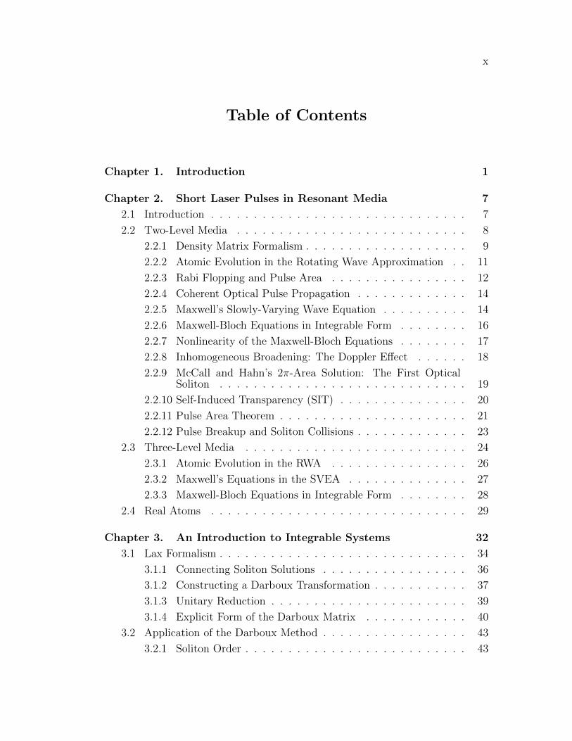
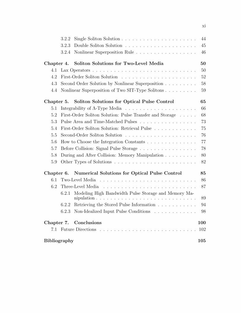
Table of Contents

Chapter 1. Introduction 1

Chapter 2. Short Laser Pulses in Resonant Media 7

2.1 Introduction . . . . . . . . . . . . . . . . . . . . . . . . . . . . . . 7

2.2 Two-Level Media . . . . . . . . . . . . . . . . . . . . . . . . . . . 8

2.2.1 Density Matrix Formalism . . . . . . . . . . . . . . . . . . . 9

2.2.2 Atomic Evolution in the Rotating Wave Approximation . . 11

2.2.3 Rabi Flopping and Pulse Area . . . . . . . . . . . . . . . . 12

2.2.4 Coherent Optical Pulse Propagation . . . . . . . . . . . . . 14

2.2.5 Maxwell’s Slowly-Varying Wave Equation . . . . . . . . . . 14

2.2.6 Maxwell-Bloch Equations in Integrable Form . . . . . . . . 16

2.2.7 Nonlinearity of the Maxwell-Bloch Equations . . . . . . . . 17

2.2.8 Inhomogeneous Broadening: The Doppler Effect . . . . . . 18

2.2.9 McCall and Hahn’s 2π-Area Solution: The First OpticalSoliton . . . . . . . . . . . . . . . . . . . . . . . . . . . . . 19

2.2.10 Self-Induced Transparency (SIT) . . . . . . . . . . . . . . . 20

2.2.11 Pulse Area Theorem . . . . . . . . . . . . . . . . . . . . . . 21

2.2.12 Pulse Breakup and Soliton Collisions . . . . . . . . . . . . . 23

2.3 Three-Level Media . . . . . . . . . . . . . . . . . . . . . . . . . . 24

2.3.1 Atomic Evolution in the RWA . . . . . . . . . . . . . . . . 26

2.3.2 Maxwell’s Equations in the SVEA . . . . . . . . . . . . . . 27

2.3.3 Maxwell-Bloch Equations in Integrable Form . . . . . . . . 28

2.4 Real Atoms . . . . . . . . . . . . . . . . . . . . . . . . . . . . . . 29

Chapter 3. An Introduction to Integrable Systems 32

3.1 Lax Formalism . . . . . . . . . . . . . . . . . . . . . . . . . . . . . 34

3.1.1 Connecting Soliton Solutions . . . . . . . . . . . . . . . . . 36

3.1.2 Constructing a Darboux Transformation . . . . . . . . . . . 37

3.1.3 Unitary Reduction . . . . . . . . . . . . . . . . . . . . . . . 39

3.1.4 Explicit Form of the Darboux Matrix . . . . . . . . . . . . 40

3.2 Application of the Darboux Method . . . . . . . . . . . . . . . . . 43

3.2.1 Soliton Order . . . . . . . . . . . . . . . . . . . . . . . . . . 43

xi

3.2.2 Single Soliton Solution . . . . . . . . . . . . . . . . . . . . . 44

3.2.3 Double Soliton Solution . . . . . . . . . . . . . . . . . . . . 45

3.2.4 Nonlinear Superposition Rule . . . . . . . . . . . . . . . . . 46

Chapter 4. Soliton Solutions for Two-Level Media 50

4.1 Lax Operators . . . . . . . . . . . . . . . . . . . . . . . . . . . . . 50

4.2 First-Order Soliton Solution . . . . . . . . . . . . . . . . . . . . . 52

4.3 Second Order Solution by Nonlinear Superposition . . . . . . . . . 58

4.4 Nonlinear Superposition of Two SIT-Type Solitons . . . . . . . . . 59

Chapter 5. Soliton Solutions for Optical Pulse Control 65

5.1 Integrability of Λ-Type Media . . . . . . . . . . . . . . . . . . . . 66

5.2 First-Order Soliton Solution: Pulse Transfer and Storage . . . . . 68

5.3 Pulse Area and Time-Matched Pulses . . . . . . . . . . . . . . . . 73

5.4 First-Order Soliton Solution: Retrieval Pulse . . . . . . . . . . . . 75

5.5 Second-Order Soliton Solution . . . . . . . . . . . . . . . . . . . . 76

5.6 How to Choose the Integration Constants . . . . . . . . . . . . . . 77

5.7 Before Collision: Signal Pulse Storage . . . . . . . . . . . . . . . . 78

5.8 During and After Collision: Memory Manipulation . . . . . . . . . 80

5.9 Other Types of Solutions . . . . . . . . . . . . . . . . . . . . . . . 82

Chapter 6. Numerical Solutions for Optical Pulse Control 85

6.1 Two-Level Media . . . . . . . . . . . . . . . . . . . . . . . . . . . 86

6.2 Three-Level Media . . . . . . . . . . . . . . . . . . . . . . . . . . 87

6.2.1 Modeling High Bandwidth Pulse Storage and Memory Ma-nipulation . . . . . . . . . . . . . . . . . . . . . . . . . . . . 89

6.2.2 Retrieving the Stored Pulse Information . . . . . . . . . . . 94

6.2.3 Non-Idealized Input Pulse Conditions . . . . . . . . . . . . 98

Chapter 7. Conclusions 100

7.1 Future Directions . . . . . . . . . . . . . . . . . . . . . . . . . . . 102

Bibliography 105

xii

List of Figures

1.1 Sketch comparing normal attenuation with short-pulse control inan absorbing dielectric medium. . . . . . . . . . . . . . . . . . . . 3

2.1 Model of a two-level atom and short-pulse propagation . . . . . . 8

2.2 Rabi flopping. . . . . . . . . . . . . . . . . . . . . . . . . . . . . . 13

2.3 Sketch of the pulse area . . . . . . . . . . . . . . . . . . . . . . . 13

2.4 Slope field diagram for the pulse Area Theorem . . . . . . . . . . 21

2.5 Pulse Area Theorem solution curves . . . . . . . . . . . . . . . . . 23

2.6 Model of a three-level atom in the Λ configuration . . . . . . . . . 25

2.7 Potential experimental realization of the theoretical Maxwell-Blochmodel with Rubidium 87 atoms. . . . . . . . . . . . . . . . . . . . 30

3.1 Illustration of the method used to produce a second-order solitonsolution. . . . . . . . . . . . . . . . . . . . . . . . . . . . . . . . . 46

3.2 Commutative Bianchi diagram for the Theorem of Permutability . 47

4.1 First-order soliton solution of the two-level Maxwell-Bloch equations 57

4.2 Pulse Rabi frequency as a function of space and time for a second-order two-pulse soliton solution . . . . . . . . . . . . . . . . . . . 62

4.3 Comparison of the pulse Rabi frequencies of a second-order two-pulse soliton solution and related first-order one-pulse solutions . 64

5.1 Relevant elements of the first-order two-pulse soliton solution inthe long negative and positive time limits. . . . . . . . . . . . . . 70

5.2 First-order two-pulse soliton solution in the limit of large, negativetime. . . . . . . . . . . . . . . . . . . . . . . . . . . . . . . . . . . 71

5.3 First-order two-pulse soliton solution at three distinct times. . . . 72

5.4 Atomic density matrix elements of the first-order two-pulse solitonsolution in the long-time limit. . . . . . . . . . . . . . . . . . . . . 73

5.5 First-order two-pulse soliton solution in the limit of large, positivetime. . . . . . . . . . . . . . . . . . . . . . . . . . . . . . . . . . . 74

5.6 Second-order three-pulse soliton solution before collision. . . . . . 79

5.7 Second-order three-pulse soliton solution during collision . . . . . 81

5.8 Quantum coherence of the second-order three-pulse soliton solu-tion at two distinct times . . . . . . . . . . . . . . . . . . . . . . . 82

5.9 Comparison of the long-time limit of our second-order three-pulsesoliton solution for three different sets of integration constants. . . 83

xiii

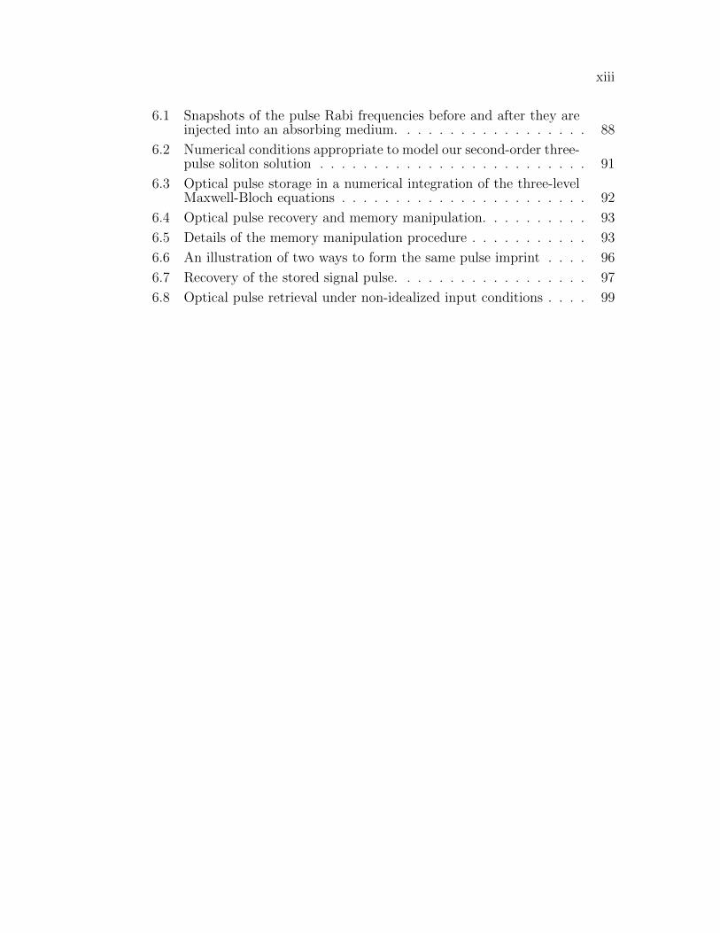
6.1 Snapshots of the pulse Rabi frequencies before and after they areinjected into an absorbing medium. . . . . . . . . . . . . . . . . . 88

6.2 Numerical conditions appropriate to model our second-order three-pulse soliton solution . . . . . . . . . . . . . . . . . . . . . . . . . 91

6.3 Optical pulse storage in a numerical integration of the three-levelMaxwell-Bloch equations . . . . . . . . . . . . . . . . . . . . . . . 92

6.4 Optical pulse recovery and memory manipulation. . . . . . . . . . 93

6.5 Details of the memory manipulation procedure . . . . . . . . . . . 93

6.6 An illustration of two ways to form the same pulse imprint . . . . 96

6.7 Recovery of the stored signal pulse. . . . . . . . . . . . . . . . . . 97

6.8 Optical pulse retrieval under non-idealized input conditions . . . . 99

1

Chapter 1

Introduction

Reliable optical communication and computation require precise control of

optical information transport. Recently, much of the progress in optical pulse con-

trol has utilized techniques involving Electromagnetically Induced Transparency

(EIT) [1]. In this phenomenon, a strong “control” pulse is injected into an absorb-

ing dielectric medium to open a narrow window in the absorption profile so that a

weak “signal” pulse at a different wavelength can pass through unattenuated. In

the region of the transparency window, the linear dispersion becomes large and

the group velocity of the signal pulse, related to the control pulse intensity, can

be much slower than the speed of light in vacuum [2, 3]. Several experiments have

been designed around modified forms of EIT to open and close the transparency

window by altering the intensity of the control field to slow and even stop, store,

and restart the signal pulse. Successful implementations of EIT-based optical

control have been achieved in cold alkali atoms [4, 5], room temperature vapors

[6–8], and solid-state systems [9]. The bandwidth of the signal pulse in these ex-

periments is limited by the narrow transparency window achievable in EIT-based

optical pulse control and some absorption of the signal pulse inevitably occurs,

reducing the fidelity of the process.

Several schemes have been proposed [10–18] to overcome bandwidth lim-

itations in order to enable higher clock rates and fast pulse-switching. Here, we

examine optical control in a new regime, where both the control and signal pulses

2

are wideband and short and no adiabatic or steady-state conditions can be as-

sociated with either field. The resonant interaction we propose allows for more

efficient light-matter coupling than Raman-based memory schemes [15–17] and

offers prospects for high-fidelity retrieval of the broadband information.

We say that an optical pulse is “stored” when it is absorbed in a process re-

sulting in a recoverable redistribution of long-lived atomic (usually ground state)

density matrix elements (the populations and off-diagonal coherences). When the

redistribution of the atomic populations can be reversed, the signal pulse can be

recovered with its original shape, intensity, and polarization faithfully restored.

We therefore say that the atomic medium stores the signal pulse information, or

contains a memory of the pulse. An essential component of the storage process

is a quantum coherence that is induced between the atomic ground state density

matrix elements and we frequently interchange the words “information,” “mem-

ory,” and “coherence” in reference to the stored signal pulse, without regard to

a rigorous, information-theoretic definition.

The high-bandwidth laser pulses we model for storage and retrieval are

assumed to be shorter than the characteristic lifetimes of the atomic states, and

the induced polarization can therefore maintain a definite phase relationship with

the field. Under such conditions, the atomic coherence can have an appreciable,

and often dramatic, effect on the incident field, and the quantum mechanical

nature of the atoms gives rise to effects that cannot be neglected. The observable

behaviors in this regime differ radically from those in the “normal” situation, as

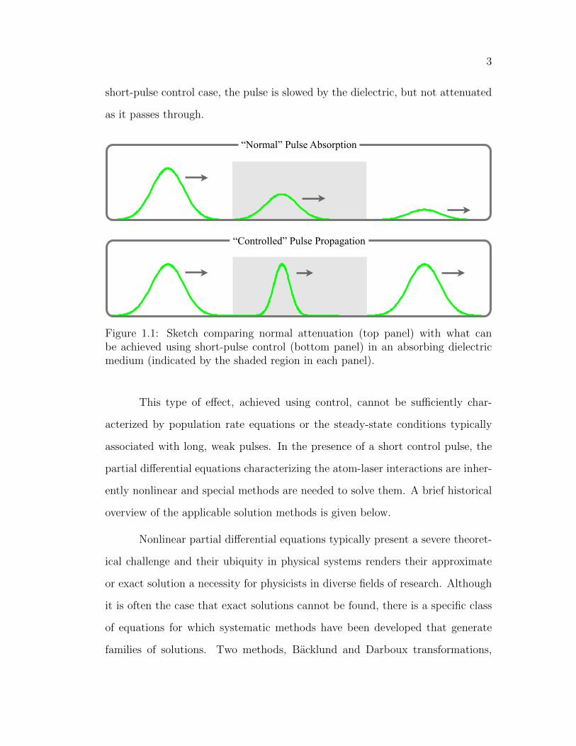
in Beer’s law of exponential absorption in a dielectric medium. A simple sketch

contrasting normal attenuation with possibilities using short-pulse “control” is

shown in Figure 1.1. In each panel, the laser pulse is shown before entering the

medium, inside the medium (shaded region), and after exiting the medium. In the

3

short-pulse control case, the pulse is slowed by the dielectric, but not attenuated

as it passes through.

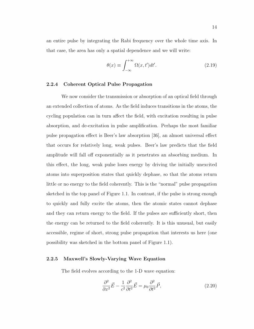
“Normal” Pulse Absorption

“Controlled” Pulse Propagation

Figure 1.1: Sketch comparing normal attenuation (top panel) with what canbe achieved using short-pulse control (bottom panel) in an absorbing dielectricmedium (indicated by the shaded region in each panel).

This type of effect, achieved using control, cannot be sufficiently char-

acterized by population rate equations or the steady-state conditions typically

associated with long, weak pulses. In the presence of a short control pulse, the

partial differential equations characterizing the atom-laser interactions are inher-

ently nonlinear and special methods are needed to solve them. A brief historical

overview of the applicable solution methods is given below.

Nonlinear partial differential equations typically present a severe theoret-

ical challenge and their ubiquity in physical systems renders their approximate

or exact solution a necessity for physicists in diverse fields of research. Although

it is often the case that exact solutions cannot be found, there is a specific class

of equations for which systematic methods have been developed that generate

families of solutions. Two methods, Backlund and Darboux transformations,

4

generate new solutions to nonlinear partial differential equations from known so-

lutions. The Backlund transformation [19] was originally developed in 1883 to

classify surfaces of negative curvature and the classical Darboux transformation

[20] was derived around the same time (in 1882) in connection with the invariance

of an ordinary differential equation. Much later, these transformations were con-

nected to nonlinear partial differential equations with important contributions

by Crum [21] and Wadati [22]. For historical information, see the monograph by

Rogers and Schief [23].

The field of nonlinear equations expanded rapidly in the late 1960s when

a method of solving the Korteweg-de Vries (KdV) equation was found [24] and

a related method was developed by Zakharov and Shabat to solve the nonlinear

Schrodinger equation [25]. The first method, now referred to as “inverse scatter-

ing,” was quickly identified as a nonlinear analog of the Fourier transform and

applied to a wide range of nonlinear evolution equations of physical significance

[26]. Lax formalized these methods in 1968 [27] and showed that the equations

they solve have commonalities. In particular, he showed that each has an as-

sociated set of operators (a “Lax pair”) that satisfy an integrability condition.

Nonlinear evolution equations with a wide range of physical applications have

since been identified as members of this class of so-called integrable equations

[28].

The type of coherent optical pulse control we study is modeled by in-

tegrable, nonlinear evolution equations and we can apply any of the aforemen-

tioned mathematical techniques to solve them. We choose to solve them exactly

using a Darboux transformation in matrix form. The matrix form of the Dar-

boux transformation was originally formulated in association with the dressing

method of Zakharov and Shabat [25] and later generalized to several different sys-

5

tems [29, 30]. Excellent descriptions of the matrix method have been prepared

by Cieslinski for non-isopectral systems from an algebraic approach (see [31, 32]

and the review article [33]) as well as by Gu, et al. using geometric methods

[28]. The advantages of the matrix Darboux transformation method are: that it

can be derived systematically and that it generates complicated solutions from

known solutions using simple integrations and algebraic methods. The type of

solutions it generates are known as soliton solutions, which we will show have

useful properties for optical pulse control.

The term soliton was originally coined by Zabusky and Kruskal [34] in

1965 to describe a solitary wave solution with particle-like properties. They nu-

merically integrated the Korteweg-deVries equation to study shallow water wave

propagation and discovered that two solitary waves could interact, or collide, and

that the smaller solitary wave was not subsumed or incorporated by the larger.

Instead, both solitary waves survived the collision, much like particles colliding

elastically. The definition of a soliton varies in the literature, as the phrase is

often used differently by applied mathematicians, physicists, and engineers. In

optical systems, for example, solitons are often assumed to be any simple solitary

wave, without any required properties under collision [35]. The first observation

of a soliton is usually attributed to the engineer Scott Russell, who chased a re-

markably stable solitary wave down a narrow channel on horseback in 1834. His

subsequent research trying to recreate the stable solitary pulse led him to discover

that the speed of the solitary waves were proportional to their height, a property

also observed much later in the numerical solutions of Zabusky and Kruskal. For

our purposes, we define a soliton solution as a particular solution to a nonlinear

equation that can be produced from a matrix Darboux transformation. We will

show that the solutions for optical pulses that we generate with this method have

6

all the classic features of soliton propagation, including survival after collision.

In the following, we derive the relevant nonlinear evolution equations for

coherent optical pulse propagation and derive the associated Darboux matrix so-

lution method. We generate three exact soliton solutions that suggest a model

for high-bandwidth optical pulse control. Our soliton solutions are derived under

unrealistic idealizations and we must test their utility in environments more rel-

evant to potential experimental realizations. To do so, we numerically integrate

the nonlinear evolution equations for finite-length media with truncated pulses of

varying shapes and areas. Our numerical and soliton solutions suggest a useful

guide for overcoming present bandwidth limits for optical pulse storage, memory

manipulation, and high-fidelity retrieval.

7

Chapter 2

Short Laser Pulses in Resonant Media

2.1 Introduction

We model the propagation of short laser pulses through an extended col-

lection of atoms with absorptive transitions. We call the laser pulses short if their

durations are shorter than the homogenous lifetimes of the relevant atomic states,

such as the timescale associated with spontaneous emission, for example. We use

a semi-classical approximation in which quantum effects are important for the

atoms but the electromagnetic field is treated classically. The field variables are

then vectors but not operators and the field must be intense enough that the loss

or gain of a few photons has a negligible effect, a condition easily met with most

laser pulses. Throughout, we assume the laser pulses can be modeled as plane

waves and that a one-dimensional analysis will suffice.

To start, we analyze a single laser pulse in an idealized absorber having

only two atomic energy states. We derive the Maxwell-Bloch equations that

describe the pulse-atom system and write them in their so-called integrable form

for use in later chapters. We also review important features of short optical

pulse propagation, including the famous Area Theorem of McCall and Hahn and

the phenomenon known as Self-Induced Transparency (SIT). Using the methods

established for single-pulse propagation, we then derive the relevant equations for

the simultaneous propagation of two laser pulses, each exciting a distinct atomic

transition in the absorber. Finally, we give an example of a real atomic system

to which our theoretical model can be applied.

8

In this document, I print the equation first in black and then in white (whichof course we can’t see on the white background)

! (1)

(2)

!3 (3)

!12 (4)

!23 (5)

(6)

23 (7)

1 (8)

loc1 (9)

0.5 (10)

|131|2 (11)

Im(13) (12)

Im(23) (13)

x (14)

t

1(15)

t/1 (16)

23 (17)

33 (18)

(19)

@

@x+

1

c

@

@t

= iµ12 (20)

@

@x+

1

c

@

@t

= iµ12 (21)

=

Z(x, t)dt (22)

1

2

1

In this document, I print the equation first in black and then in white (whichof course we can’t see on the white background)

!13 (1)

!23 (2)

(3)

23 (4)

1 (5)

loc1 (6)

0.5 (7)

|131|2 (8)

Im(13) (9)

Im(23) (10)

x (11)

t

1(12)

t/1 (13)

23 (14)

33 (15)

(16)

@

@x+

1

c

@

@t

= iµ12 (17)

@

@x+

1

c

@

@t

= iµ12 (18)

=

Z(x, t)dt (19)

=

Z(x, t)dt (20)

vg =c

1 + (21)

1

Controlled Pulse Propagation

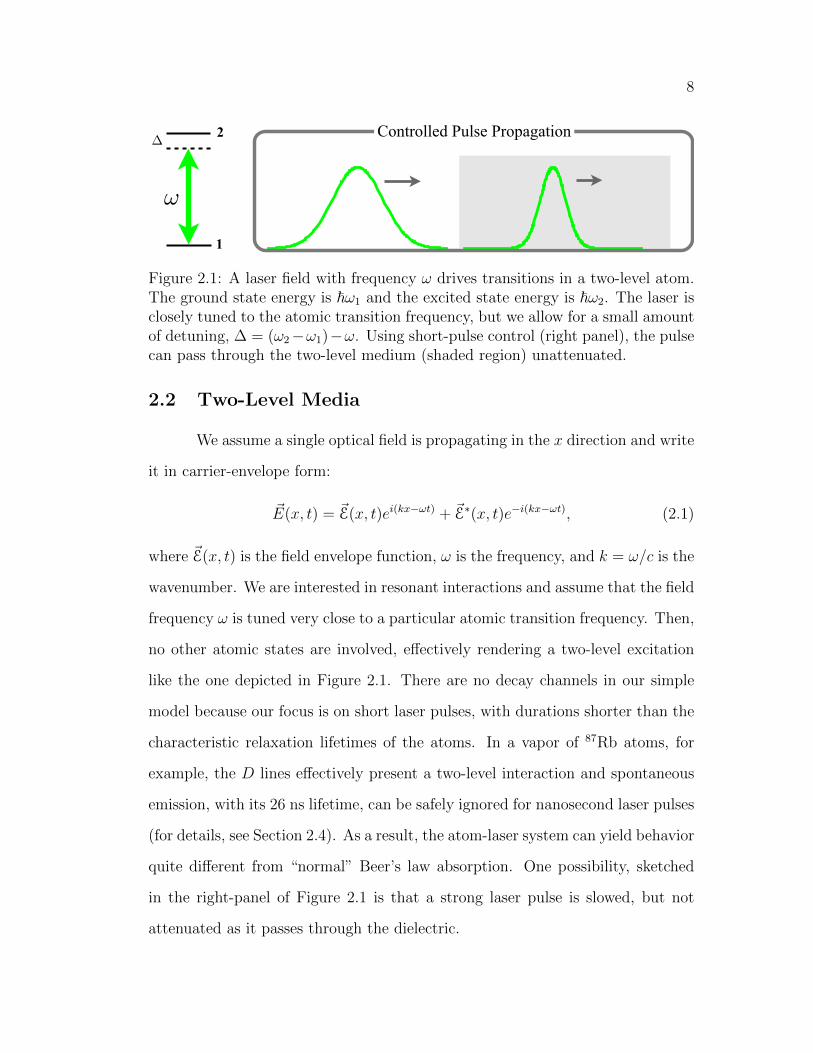
Figure 2.1: A laser field with frequency ω drives transitions in a two-level atom.The ground state energy is ~ω1 and the excited state energy is ~ω2. The laser isclosely tuned to the atomic transition frequency, but we allow for a small amountof detuning, ∆ = (ω2−ω1)−ω. Using short-pulse control (right panel), the pulsecan pass through the two-level medium (shaded region) unattenuated.

2.2 Two-Level Media

We assume a single optical field is propagating in the x direction and write

it in carrier-envelope form:

~E(x, t) = ~E(x, t)ei(kx−ωt) + ~E∗(x, t)e−i(kx−ωt), (2.1)

where ~E(x, t) is the field envelope function, ω is the frequency, and k = ω/c is the

wavenumber. We are interested in resonant interactions and assume that the field

frequency ω is tuned very close to a particular atomic transition frequency. Then,

no other atomic states are involved, effectively rendering a two-level excitation

like the one depicted in Figure 2.1. There are no decay channels in our simple

model because our focus is on short laser pulses, with durations shorter than the

characteristic relaxation lifetimes of the atoms. In a vapor of 87Rb atoms, for

example, the D lines effectively present a two-level interaction and spontaneous

emission, with its 26 ns lifetime, can be safely ignored for nanosecond laser pulses

(for details, see Section 2.4). As a result, the atom-laser system can yield behavior

quite different from “normal” Beer’s law absorption. One possibility, sketched

in the right-panel of Figure 2.1 is that a strong laser pulse is slowed, but not

attenuated as it passes through the dielectric.

9

We label the energies of the atomic ground and excited states by ~ω1

and ~ω2, respectively. Then, in the energy eigenbasis, |1〉, |2〉, the atom-laser

Hamiltonian is:

H = ~ω1 |1〉 〈1|+ ~ω2 |2〉 〈2| − ~d · ~E, (2.2)

under the dipole approximation. The atomic dipole moment operator is:

~d = ~d12 |1〉 〈2|+ ~d21 |2〉 〈1| . (2.3)

If we assume the atomic state can be represented by a wavefunction, |ψ〉, then it

evolves according to Schrodinger’s equation:

i~∂

∂t|ψ〉 = H |ψ〉 , (2.4)

and we can write the wavefunction for the two-level atom in the energy eigenbasis:

|ψ(t)〉 = c1(t) |1〉+ c2(t) |2〉 , (2.5)

for the time-dependent probability amplitudes of levels 1 and 2, c1(t) and c2(t),

respectively.

2.2.1 Density Matrix Formalism

Real media often cannot be sufficiently described by a single wavefunction

and, in that case, a more general formalism is needed. For example, atoms within

an ensemble undergo many soft, phase-changing collisions which can affect the

dipole oscillations of the atoms but leave the populations unchanged. To account

for such an effect, we specify the atomic state by the density matrix, ρ, a positive,

Hermitian operator of unit trace:

ρ =

(ρ11 ρ12

ρ21 ρ22

), (2.6)

10

written in the energy eigenbasis with column ordering |1〉 , |2〉. In general, the

density matrix is a function of both space and time, but we typically suppress

that dependence for notational convenience, meaning ρ12 = ρ12(x, t).

In the special case of a pure state, the density matrix is related to the

wavefunction through the outer product:

ρ = |ψ〉 〈ψ| =(|c1|2 c1c

∗2

c∗1c2 |c2|2). (pure state)

The diagonal elements of the density matrix, ρ11 and ρ22, are the populations

of levels 1 and 2, respectively, and the off-diagonal element ρ12 = c1c∗2 is the

coherence between them. When the atom cannot be characterized by a single

wavefunction, the off-diagonal element of the density matrix, ρ12, may have no

direct relationship to the diagonal-elements ρ11 and ρ22 and, in such a case, we say

the atom is in a mixed state. The density matrix can describe a much wider range

of atomic behavior than the wavefunction, including media that have suffered a

complete loss of all coherence (ρ12 = 0) but whose populations are intact. To

model this type of media, the density matrix would be written:

ρ =

(ρ11 00 ρ22

). (2.7)

One can easily verify that this so-called fully mixed state cannot be constructed

from a single wavefunction.

For both mixed and pure states, the density matrix must have unit trace

(ρ11 +ρ22 = 1) so that probability is conserved in our closed system. The density

matrix evolves according to the von Neumann equation:

i~∂

∂tρ = [H, ρ]. (2.8)

The brackets denote commutation between the matrix operators, [H, ρ] = Hρ−

11

ρH and, in matrix form, the atom-laser Hamiltonian is:

H =

(~ω1 −~d · ~E−~d∗ · ~E ~ω2

), (2.9)

with column ordering |1〉, |2〉. One can easily check that the von Neumann

equation reduces to the Schrodinger equation for a pure state.

2.2.2 Atomic Evolution in the Rotating Wave Approximation

We are interested in solutions to the von Neumann equation under the so-

called rotating wave approximation (RWA), in which we neglect fast-oscillating

terms to simplify the Hamiltonian. To identify which terms can be reasonably

replaced by their zero-average values, we first transform to a new, rotating basis.

To do so, we apply the unitary transformation matrix:

U = eiω1t

(1 00 e−i(kx−ωt)

). (2.10)

The density matrix transforms as:

ρRW = UρU †, (2.11)

where the RW superscript indicates the rotating wave basis. One can show that

the von Neumann equation is form-invariant under the unitary transformation:

i~∂

∂tρRW = [HRW, ρRW], (2.12)

by identifying the Hamiltonian in the rotating wave basis as:

HRW = UHU † + i~(∂

∂tU)U †. (2.13)

In terms of the detuning, ∆ = (ω2 − ω1)− ω, the Hamiltonian in this basis is:

HRW =

(0 −(~d12 · ~E)ei(kx−ωt)

−(~d21 · ~E)e−i(kx−ωt) ~∆

). (2.14)

12

Notice from definition (2.1) of the electric field that the right off-diagonal term

contains ~Eei(kx−ωt) = ~Ee2i(kx−ωt) + ~E∗ and the left off-diagonal term contains

~Ee−i(kx−ωt) = ~E + ~Ee−2i(kx−ωt). In making the rotating wave approximation, we

neglect the fast-oscillating ±2iωt terms, assuming that the envelope function

~E(x, t) varies slowly compared to the carrier wave. This assumption is easily met

for the pulses we are interested in; a 0.1 ns pulse, for example, contains on the

order of 104 optical cycles. Using this approximation, we find the Hamiltonian

in the RWA:

HRWA =

(0 −~d12 · ~E∗

−~d21 · ~E ~∆

)=

(0 −~

2Ω∗

−~2Ω ~∆

). (2.15)

In the above, we have identified the Rabi frequency,

Ω(x, t) ≡ 2~d21 · ~E(x, t)

~. (2.16)

The Rabi frequency plays an important role in atom-laser systems, as it incorpo-

rates both the atomic dipole moment operator and the slowly-varying envelope of

the field. The ~ in the denominator of the Rabi frequency hints that there is no

classical ~ → 0 analog and we will find that our semi-classical approach retains

quantum features of the system.

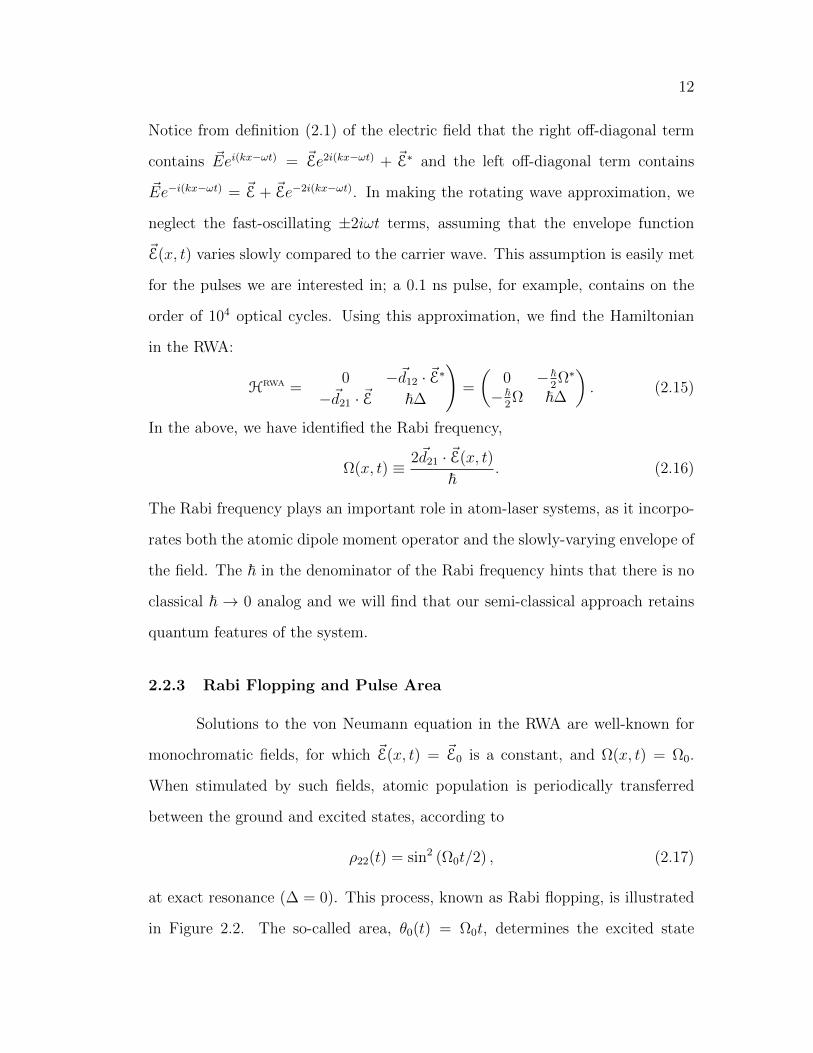
2.2.3 Rabi Flopping and Pulse Area

Solutions to the von Neumann equation in the RWA are well-known for

monochromatic fields, for which ~E(x, t) = ~E0 is a constant, and Ω(x, t) = Ω0.

When stimulated by such fields, atomic population is periodically transferred

between the ground and excited states, according to

ρ22(t) = sin2 (Ω0t/2) , (2.17)

at exact resonance (∆ = 0). This process, known as Rabi flopping, is illustrated

in Figure 2.2. The so-called area, θ0(t) = Ω0t, determines the excited state

13

p 2 p 3 p 4 p 5 p 6 p

0.5

1

W0t

(x, t) (1)

22 (2)

x = 0 (3)

ln R00 (4)

13a (5)

x2 = (6)

t/a (7)

x2 = 6.5600 (8)

x2 = x1 + ab = 6.6593 (9)

a12 (10)

ln |R1| (11)

x1 = ln R0 = 3.0000 (12)

|13/23| = R00 (13)

1/b (14)

(a12 + ab) (15)

a1 = 1, a2 = 5, a3 = i/5, (16)

a1 = 1, a2 = 5, a3 =1

5i, (17)

b1 = 0, b2 = 1, b3 = i, (18)

a = 2 b = 1, T = 25a, (19)

a1 = 1, a2 = 5, a3 =1

5i, (20)

b1 = 0, b2 = 1, b3 = i, (21)

a1 = 1 (22)

a2 = 2 (23)

aab13 (24)

↵x/2 (25)

1

Rabi Flopping

Figure 2.2: For a constant field, the atom is periodically excited at a fixed ratedetermined by the pulse area Ω0t.

0 t t¢

(x, t0) (1)

22 (2)

x = 0 (3)

ln R00 (4)

13a (5)

x2 = (6)

t/a (7)

x2 = 6.5600 (8)

x2 = x1 + ab = 6.6593 (9)

a12 (10)

ln |R1| (11)

x1 = ln R0 = 3.0000 (12)

|13/23| = R00 (13)

1/b (14)

(a12 + ab) (15)

a1 = 1, a2 = 5, a3 = i/5, (16)

a1 = 1, a2 = 5, a3 =1

5i, (17)

b1 = 0, b2 = 1, b3 = i, (18)

a = 2 b = 1, T = 25a, (19)

a1 = 1, a2 = 5, a3 =1

5i, (20)

b1 = 0, b2 = 1, b3 = i, (21)

a1 = 1 (22)

a2 = 2 (23)

aab13 (24)

↵x/2 (25)

1

Pulse Area

(x, t) (1)

22 (2)

x = 0 (3)

ln R00 (4)

13a (5)

x2 = (6)

t/a (7)

x2 = 6.5600 (8)

x2 = x1 + ab = 6.6593 (9)

a12 (10)

ln |R1| (11)

x1 = ln R0 = 3.0000 (12)

|13/23| = R00 (13)

1/b (14)

(a12 + ab) (15)

a1 = 1, a2 = 5, a3 = i/5, (16)

a1 = 1, a2 = 5, a3 =1

5i, (17)

b1 = 0, b2 = 1, b3 = i, (18)

a = 2 b = 1, T = 25a, (19)

a1 = 1, a2 = 5, a3 =1

5i, (20)

b1 = 0, b2 = 1, b3 = i, (21)

a1 = 1 (22)

a2 = 2 (23)

aab13 (24)

↵x/2 (25)

1

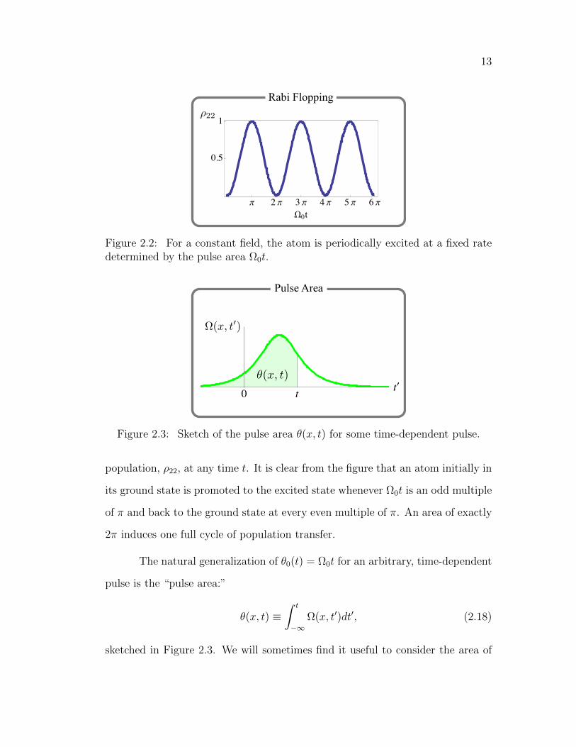
Figure 2.3: Sketch of the pulse area θ(x, t) for some time-dependent pulse.

population, ρ22, at any time t. It is clear from the figure that an atom initially in

its ground state is promoted to the excited state whenever Ω0t is an odd multiple

of π and back to the ground state at every even multiple of π. An area of exactly

2π induces one full cycle of population transfer.

The natural generalization of θ0(t) = Ω0t for an arbitrary, time-dependent

pulse is the “pulse area:”

θ(x, t) ≡∫ t

−∞Ω(x, t′)dt′, (2.18)

sketched in Figure 2.3. We will sometimes find it useful to consider the area of

14

an entire pulse by integrating the Rabi frequency over the whole time axis. In

that case, the area has only a spatial dependence and we will write:

θ(x) ≡∫ +∞

−∞Ω(x, t′)dt′. (2.19)

2.2.4 Coherent Optical Pulse Propagation

We now consider the transmission or absorption of an optical field through

an extended collection of atoms. As the field induces transitions in the atoms, the

cycling population can in turn affect the field, with excitation resulting in pulse

absorption, and de-excitation in pulse amplification. Perhaps the most familiar

pulse propagation effect is Beer’s law absorption [36], an almost universal effect

that occurs for relatively long, weak pulses. Beer’s law predicts that the field

amplitude will fall off exponentially as it penetrates an absorbing medium. In

this effect, the long, weak pulse loses energy by driving the initially unexcited

atoms into superposition states that quickly dephase, so that the atoms return

little or no energy to the field coherently. This is the “normal” pulse propagation

sketched in the top panel of Figure 1.1. In contrast, if the pulse is strong enough

to quickly and fully excite the atoms, then the atomic states cannot dephase

and they can return energy to the field. If the pulses are sufficiently short, then

the energy can be returned to the field coherently. It is this unusual, but easily

accessible, regime of short, strong pulse propagation that interests us here (one

possibility was sketched in the bottom panel of Figure 1.1).

2.2.5 Maxwell’s Slowly-Varying Wave Equation

The field evolves according to the 1-D wave equation:

∂2

∂x2~E − 1

c2

∂2

∂t2~E = µ0

∂2

∂t2~P , (2.20)

15

where ~P is the (space and time dependent) polarization. For a dielectric medium

of two-level atoms with number density N, the polarization is:

~P = N Trace( ~d ρ), (2.21a)

= N(~d12 ρ21 + ~d21 ρ12

), (2.21b)

= N(~d12 ρ

RW

21 e−i(kx−ωt) + ~d21 ρ

RW

12 ei(kx−ωt)

). (2.21c)

In the last line, we have written the polarization in the rotating wave variables

defined in Section 2.2.2. Taking the derivatives and collecting same-frequency

terms in Maxwell’s wave equation, we find:

(−k2~E + 2ik

∂

∂x~E +

∂

∂x2~E

)− 1

c2

(−ω2~E− 2iω

∂

∂t~E +

∂2

∂t2~E

)

= N~d12

(−ω2ρRW

21 − 2iω∂

∂tρRW

21 +∂2

∂t2ρRW

21

) (2.22)

To proceed, we again assume the field varies slowly compared to the carrier wave

and therefore make the slowly-varying envelope approximation (SVEA), under

which: ∣∣∣∣∂E

∂x

∣∣∣∣ k |E| ,∣∣∣∣∂2E

∂x2

∣∣∣∣ k

∣∣∣∣∂E

∂x

∣∣∣∣ ,∣∣∣∣∂2E

∂t2

∣∣∣∣ ω2 |E| . (2.23)

Similarly, the rotating-wave variables are slowly-varying by definition:

∣∣∣∣∂ρRW

12

∂t

∣∣∣∣ ω |ρRW

12 | . (2.24)

Adopting the SVEA and RWA and noting that k = ω/c, we find Maxwell’s

slowly-varying equation:

2

(∂

∂x+

1

c

∂

∂t

)~E =

iω

ε0cN~d12ρ

RW

21 , (2.25)

or, in terms of the Rabi frequency,

(∂

∂x+

1

c

∂

∂t

)Ω = iµρRWA

21 . (2.26)

16

In the above, we have identified

µ ≡ Nω|d12|2~ε0c

, (2.27)

as the atom-field coupling parameter. Collectively, equations (2.8) and (2.26) are

referred to as the Maxwell-Bloch equations. We will work exclusively in the RWA

and SVEA and will drop the RWA superscript hereafter.

2.2.6 Maxwell-Bloch Equations in Integrable Form

Here, we rewrite the Maxwell-Bloch equations in a more symmetric form,

important for solving them with the methods described in the next chapter. We

start by writing Maxwell’s slowly-varying equation in terms of the Hamiltonian

by defining a constant matrix

W = i |2〉 〈2| =(

0 00 i

). (2.28)

Then, equation (2.26) is equivalent to:

(∂

∂x+

1

c

∂

∂t

)H = −~µ

2[W, ρ]. (2.29)

Next, we define the traveling-wave coordinates T = t−x/c, Z = x, for which the

derivatives transform as:

∂

∂T→ ∂

∂t,

∂

∂Z→ ∂

∂x+

1

c

∂

∂t. (2.30)

In these coordinates, the Maxwell-Bloch equations are:

i~∂ρ

∂T= [H, ρ], (2.31a)

∂H

∂Z= −~µ

2[W, ρ]. (2.31b)

We will use this form of the Maxwell-Bloch equations in Chapter 3 to show that

the two-level atom-laser system is exactly integrable with soliton solutions.

17

2.2.7 Nonlinearity of the Maxwell-Bloch Equations

In the above, we have claimed that we need special solution methods to

solve the Maxwell-Bloch equations due to their nonlinearity. It is not at all ob-

vious that this system of equations is in fact nonlinear because, when viewed

separately, both the von-Neumann equation and Maxwell’s slowly-varying equa-

tion are linear. The nonlinearity of the system arises because of the coupling of

these two equations. In the special case of a pure atomic state and a real Rabi

frequency, we can expose the nonlinearity by using the linear equations to derive

a single equation for the pulse area.

For a pure state, |ψ〉 = c1 |1〉 + c2 |2〉, we have ρ21 = c∗1c2 and Maxwell’s

slowly-varying equation (2.26) in the traveling-wave coordinates is:

∂Ω

∂Z= iµc∗1c2. (2.32)

The Rabi frequency can be written in terms of the pulse area by:

∂θ

∂T= Ω, (2.33)

and substituting this into the above, we find:

∂2θ

∂Z∂T= iµc∗1c2. (2.34)

To write the probability amplitudes c1, c2 in terms of the pulse area, we use the

von Neumann equation, which reduces to Schrodinger’s equation for a pure state.

For the two-level atom with zero detuning, ∆ = 0, in the traveling-wave

coordinates, Schrodinger’s equation states that:

i~∂

∂T

(c1

c2

)= −~

2

(0 ΩΩ 0

)(c1

c2

), (2.35)

or, in terms of the pulse area:

i~∂

∂T

(c1

c2

)= −~

2

∂θ

∂T

(0 11 0

)(c1

c2

). (2.36)

18

The relevant equation is therefore simply:

∂

∂θ

(c1

c2

)=i

2

(0 11 0

)(c1

c2

). (2.37)

If the dielectric is prepared in its ground state, then the appropriate initial con-

ditions are: c2(0) = 0, c1(0) = 1 (this is for θ = 0, meaning the atomic state at

T = −∞, before the pulse arrives). The solution for the level amplitudes is then:

c1(θ) = cosθ

2, (2.38a)

c2(θ) = i sinθ

2. (2.38b)

Applying this result to equation (2.34), we find:

∂2θ

∂Z∂T= −µ

2sin θ. (2.39)

The nonlinearity of the coupled Maxwell-Bloch equations is clearly evident in

this equation, the so-called Sine-Gordon equation [37].

2.2.8 Inhomogeneous Broadening: The Doppler Effect

In real media, there is a variety of reasons why the effective resonant

transition frequency may differ from atom to atom, including impurities and in-

homogeneous strain fields, for example. The dominant mechanism in the systems

we study is the Doppler effect, in which differing atomic velocities lead to dif-

fering resonant frequencies from the point of view of the laser. To account for

inhomogeneous broadening of this type, we must average over the polarizations

in Maxwell’s equation:

〈ρ12〉 ≡∫ρ12F (∆)d∆. (2.40)

The appropriate distribution function, F (∆), can be derived from the Maxwell-

Boltzmann distribution for gases. In terms of the detunings, it is:

F (∆) =T ∗2√2πe−(∆−∆)2(T ∗

2 )2/2 (2.41)

19

where T ∗2 is the Doppler lifetime and ∆ is the line-center detuning.

2.2.9 McCall and Hahn’s 2π-Area Solution: The First Optical Soliton

In Chapter 3, we will discuss soliton theory in detail and develop a method

to produce such solutions systematically. Here, we briefly review the behavior of a

particular soliton solution that highlights some of the most interesting aspects of

short optical pulse propagation in two-level media. McCall and Hahn found that

an inhomogeneously broadened medium can support a pulse with Rabi frequency:

Ω =2

τsech

(x/vg − t

τ

), (2.42)

where τ is the nominal pulse duration while the pulse group velocity is:

vg =c

(1 + κτ/2). (2.43)

The absorption coefficient:

κ =µc

2τ

∫ ∞

−∞

F (∆)d∆

∆2 + (1/τ)2, (2.44)

accounts for a spread of the detunings through the distribution function F (∆)

and the group velocity vg may be much slower than the speed of light in vacuum.

The density matrix elements associated with this Rabi frequency depend

directly on the detuning, ∆, and for ∆ = 0, they are:

ρ11 = tanh2

(x/vg − t

τ

), (2.45a)

ρ22 = sech2

(x/vg − t

τ

), (2.45b)

ρ12 = i sech

(x/vg − t

τ

)tanh

(x/vg − t

τ

), (2.45c)

and one easily checks that ρ11 + ρ22 = 1. This solution describes a medium of

atoms initially in their ground state before the pulse arrives.

20

As previously noted, such a medium is absorbing for long, weak pulses

and a resonant field would be depleted within a few absorption depths according

to Beer’s law. In our contrasting regime of short, strong pulses, the optical pulse

propagates at velocity vg without depletion. The pulse is strong enough to drive

the atoms to the excited state and short enough for the atoms to return the

energy back to the field coherently. The atoms are returned to the ground state

after excitation and it is therefore not surprising that the area of the pulse is

exactly 2π:

θ(x) =

∫ ∞

−∞Ω(x, t)dt =

2

τ

∫ ∞

−∞sech

(x/vg − t

τ

)dt = 2π. (2.46)

2.2.10 Self-Induced Transparency (SIT)

What is remarkable about the solution above is that the careful balancing

of pulse absorption and amplification via the nonlinear interaction it suggests has

been observed in the laboratory and is exhibited even for non-idealized input pulse

shapes and areas [38]. That is, if a non-idealized input pulse is strong enough

to excite a significant fraction of the atoms, then the coherent exchange between

those atoms and the field reshapes the laser pulse until it has a hyperbolic secant

shape with pulse area equal to 2π. Electromagnetically Induced Transparency

(EIT) is a related effect for three-level atoms that requires two pulses, one of which

opens a transparency window in the absorption profile of the other. In contrast,

here the pulse itself opens the transparency window that makes absorptionless

propagation possible and the phenomenon is appropriately referred to as Self-

Induced Transparency (SIT).

21

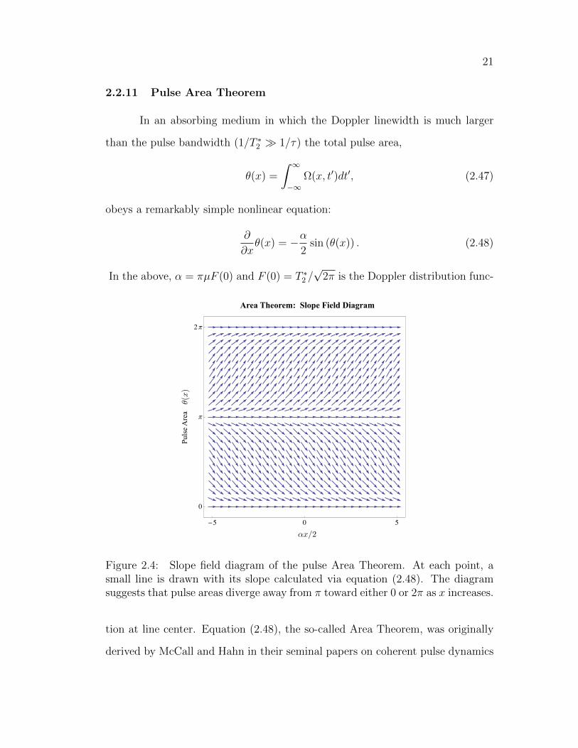
2.2.11 Pulse Area Theorem

In an absorbing medium in which the Doppler linewidth is much larger

than the pulse bandwidth (1/T ∗2 1/τ) the total pulse area,

θ(x) =

∫ ∞

−∞Ω(x, t′)dt′, (2.47)

obeys a remarkably simple nonlinear equation:

∂

∂xθ(x) = −α

2sin (θ(x)) . (2.48)

In the above, α = πµF (0) and F (0) = T ∗2 /√

2π is the Doppler distribution func-

Area Theorem: Slope Field Diagram

-5 0 5

0

p

2 p

aa

In this document, I print the equation first in black and then in white (whichof course we can’t see on the white background)

↵x

2(1)

↵x/2 (2)

! (3)

(4)

!3 (5)

!12 (6)

!23 (7)

(8)

23 (9)

1 (10)

loc1 (11)

0.5 (12)

|131|2 (13)

Im(13) (14)

Im(23) (15)

x (16)

t

1(17)

t/1 (18)

23 (19)

33 (20)

(21)

@

@x+

1

c

@

@t

= iµ12 (22)

@

@x+

1

c

@

@t

= iµ12 (23)

1

Puls

e Are

a

Inth

isdocu

men

t,Ipri

ntth

eeq

uati

on

firs

tin

bla

ckand

then

inw

hit

e(w

hic

hofco

urs

ew

eca

n’t

see

on

the

whit

eback

gro

und)

(x

)(1

)

↵x/2

(2)

!(3

)

(4

)

!3

(5)

!12

(6)

!23

(7)

(8

)

23

(9)

1(1

0)

loc 1

(11)

0.5

(12)

|13 1

|2(1

3)

Im(

13)

(14)

Im(

23)

(15)

x

(16)

t 1(1

7)

t/ 1

(18)

23

(19)

33

(20)

(2

1)

@ @x

+1 c

@ @t

=

iµ12

(22)

@ @x

+1 c

@ @t

=

iµ12

(23)

1

Figure 2.4: Slope field diagram of the pulse Area Theorem. At each point, asmall line is drawn with its slope calculated via equation (2.48). The diagramsuggests that pulse areas diverge away from π toward either 0 or 2π as x increases.

tion at line center. Equation (2.48), the so-called Area Theorem, was originally

derived by McCall and Hahn in their seminal papers on coherent pulse dynamics

22

[38, 39]. Their remarkable “theorem” offers useful predictions about the system

dynamics without reference to any specific pulse shape.

For example, it is immediately apparent from equation (2.48) that pulse

areas that are integer multiples of π will remain constant because (∂/∂x)θ(x) =

0. In addition, for small areas that satisfy sin θ(x) ≈ θ(x), the Area Theorem

becomes linear and predicts exponential absorption of the pulse. Small area

pulses are thus absorbed as in Beer’s law and, in this regime, the absorption

coefficient depends on the pulse duration τ acting as an effective homogeneous

linewidth.

The tendency of pulse areas toward 0π is not restricted to weak pulse

propagation, as one can see from the slope field diagram in Figure 2.4. The

figure shows that pulses with areas just below π tend toward 0π with increasing

penetration into the medium. Pulses with areas just greater than π, however,

tend toward 2π asymptotically. These features are true more generally. In short-

pulse propagation in absorbing media, the even multiples of π are stable solutions

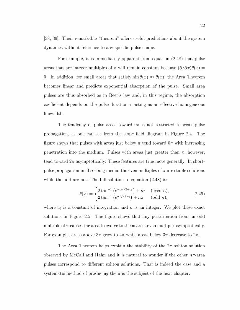
while the odd are not. The full solution to equation (2.48) is:

θ(x) =

2 tan−1

(e−αx/2+c0

)+ nπ (even n),

2 tan−1(eαx/2+c0

)+ nπ (odd n),

(2.49)

where c0 is a constant of integration and n is an integer. We plot these exact

solutions in Figure 2.5. The figure shows that any perturbation from an odd

multiple of π causes the area to evolve to the nearest even multiple asymptotically.

For example, areas above 3π grow to 4π while areas below 3π decrease to 2π.

The Area Theorem helps explain the stability of the 2π soliton solution

observed by McCall and Hahn and it is natural to wonder if the other nπ-area

pulses correspond to different soliton solutions. That is indeed the case and a

systematic method of producing them is the subject of the next chapter.

23

Puls

e Are

a

-15 -10 -5 0 5 10 15-4 p

-3 p

-2 p

-p

0

p

2 p

3 p

4 p

Pulse Area Theorem: Solutions

a

In this document, I print the equation first in black and then in white (whichof course we can’t see on the white background)

↵x

2(1)

↵x/2 (2)

! (3)

(4)

!3 (5)

!12 (6)

!23 (7)

(8)

23 (9)

1 (10)

loc1 (11)

0.5 (12)

|131|2 (13)

Im(13) (14)

Im(23) (15)

x (16)

t

1(17)

t/1 (18)

23 (19)

33 (20)

(21)

@

@x+

1

c

@

@t

= iµ12 (22)

@

@x+

1

c

@

@t

= iµ12 (23)

1

Inth

isdocu

men

t,Ipri

ntth

eeq

uati

on

firs

tin

bla

ckand

then

inw

hit

e(w

hic

hofco

urs

ew

eca

n’t

see

on

the

whit

eback

gro

und)

(x

)(1

)

↵x/2

(2)

!(3

)

(4

)

!3

(5)

!12

(6)

!23

(7)

(8

)

23

(9)

1(1

0)

loc 1

(11)

0.5

(12)

|13 1

|2(1

3)

Im(

13)

(14)

Im(

23)

(15)

x

(16)

t 1(1

7)

t/ 1

(18)

23

(19)

33

(20)

(2

1)

@ @x

+1 c

@ @t

=

iµ12

(22)

@ @x

+1 c

@ @t

=

iµ12

(23)

1

Figure 2.5: Solutions curves for the pulse Area Theorem. The curves are drawnfrom equation (2.49) with n = 2, 0,−2,−4 (green lines, top to bottom) andn = 3, 1,−1,−3 (purple lines, top to bottom). The solutions tend away from oddmultiples of π and toward the even multiples.

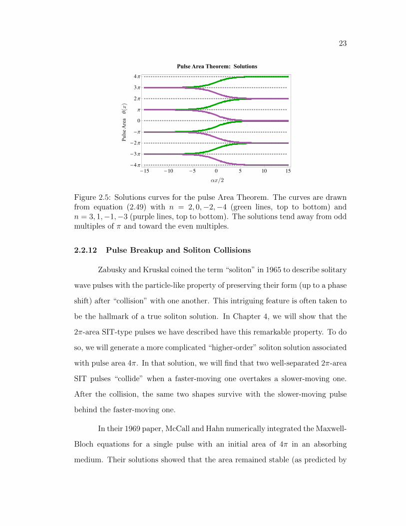
2.2.12 Pulse Breakup and Soliton Collisions

Zabusky and Kruskal coined the term “soliton” in 1965 to describe solitary

wave pulses with the particle-like property of preserving their form (up to a phase

shift) after “collision” with one another. This intriguing feature is often taken to

be the hallmark of a true soliton solution. In Chapter 4, we will show that the

2π-area SIT-type pulses we have described have this remarkable property. To do

so, we will generate a more complicated “higher-order” soliton solution associated

with pulse area 4π. In that solution, we will find that two well-separated 2π-area

SIT pulses “collide” when a faster-moving one overtakes a slower-moving one.

After the collision, the same two shapes survive with the slower-moving pulse

behind the faster-moving one.

In their 1969 paper, McCall and Hahn numerically integrated the Maxwell-

Bloch equations for a single pulse with an initial area of 4π in an absorbing

medium. Their solutions showed that the area remained stable (as predicted by

24

the Area Theorem), but that the large pulse quickly broke up into two 2π-area

SIT-type pulses. After this “pulse breakup,” the 2π-area pulses propagated un-

changed, each inducing one full cycle of the atomic population. By injecting

a large, 4π-area pulse initially, McCall and Hahn were essentially simulating a

collision between two 2π-area pulses. Their initial conditions can be associated

with a time in the 4π-area solution at which the two 2π-area pulses have col-

lided and are overlapped. Similarly, a 6π-area pulse can be associated with a

soliton solution in which three 2π-area SIT-type pulses have collided and so on.

After collision (or breakup), each 2π-area pulse propagates unchanged, inducing

successive cycles of atomic excitation and de-excitation one after the other.

2.3 Three-Level Media

We have seen that the hyperbolic secant pulse is a particularly important

shape in resonant two-level interactions and may expect it to be relevant in

more complicated, multi-level systems. However, atoms with additional energy

levels and multiple optical pulses driving transitions between them afford the

opportunity for more control over the medium and its response, allowing for

more complicated behaviors. In this section, we derive the governing nonlinear

evolution equations under the RWA and SVEA for a two-pulse three-level atomic

system in the Λ-configuration illustrated in Figure 2.6. We assume each pulse

addresses a single atomic transition frequency and will refer to the field tuned to

the 1-3 transition as the signal pulse and the field tuned to the 2-3 frequency as

the control pulse. We write the sum of the two fields in carrier-envelope form as:

~E(x, t) = ~E13(x, t) ei(k13x−ω13t) + ~E23(x, t) ei(k23x−ω23t) + c.c., (2.50)

where ω13 and ω23 are the field frequencies, while k13 = ω13/c and k23 = ω23/c

are the wavenumbers, and ~E13(x, t) and ~E23(x, t) are the slowly-varying field en-

25

1

3

2

In this document, I print the equation first in black and then in white (whichof course we can’t see on the white background)

!13 (1)

!23 (2)

(3)

23 (4)

1 (5)

loc1 (6)

0.5 (7)

|131|2 (8)

Im(13) (9)

Im(23) (10)

x (11)

t

1(12)

t/1 (13)

23 (14)

33 (15)

(16)

@

@x+

1

c

@

@t

= iµ12 (17)

@

@x+

1

c

@

@t

= iµ12 (18)

=

Z(x, t)dt (19)

=

Z(x, t)dt (20)

vg =c

1 + (21)

1

In this document, I print the equation first in black and then in white (whichof course we can’t see on the white background)

!13 (1)

!23 (2)

(3)

23 (4)

1 (5)

loc1 (6)

0.5 (7)

|131|2 (8)

Im(13) (9)

Im(23) (10)

x (11)

t

1(12)

t/1 (13)

23 (14)

33 (15)

(16)

@

@x+

1

c

@

@t

= iµ12 (17)

@

@x+

1

c

@

@t

= iµ12 (18)

=

Z(x, t)dt (19)

=

Z(x, t)dt (20)

vg =c

1 + (21)

1

In this document, I print the equation first in black and then in white (whichof course we can’t see on the white background)

!13 (1)

!23 (2)

(3)

23 (4)

1 (5)

loc1 (6)

0.5 (7)

|131|2 (8)

Im(13) (9)

Im(23) (10)

x (11)

t

1(12)

t/1 (13)

23 (14)

33 (15)

(16)

@

@x+

1

c

@

@t

= iµ12 (17)

@

@x+

1

c

@

@t

= iµ12 (18)

=

Z(x, t)dt (19)

=

Z(x, t)dt (20)

vg =c

1 + (21)

1

signalcontrol

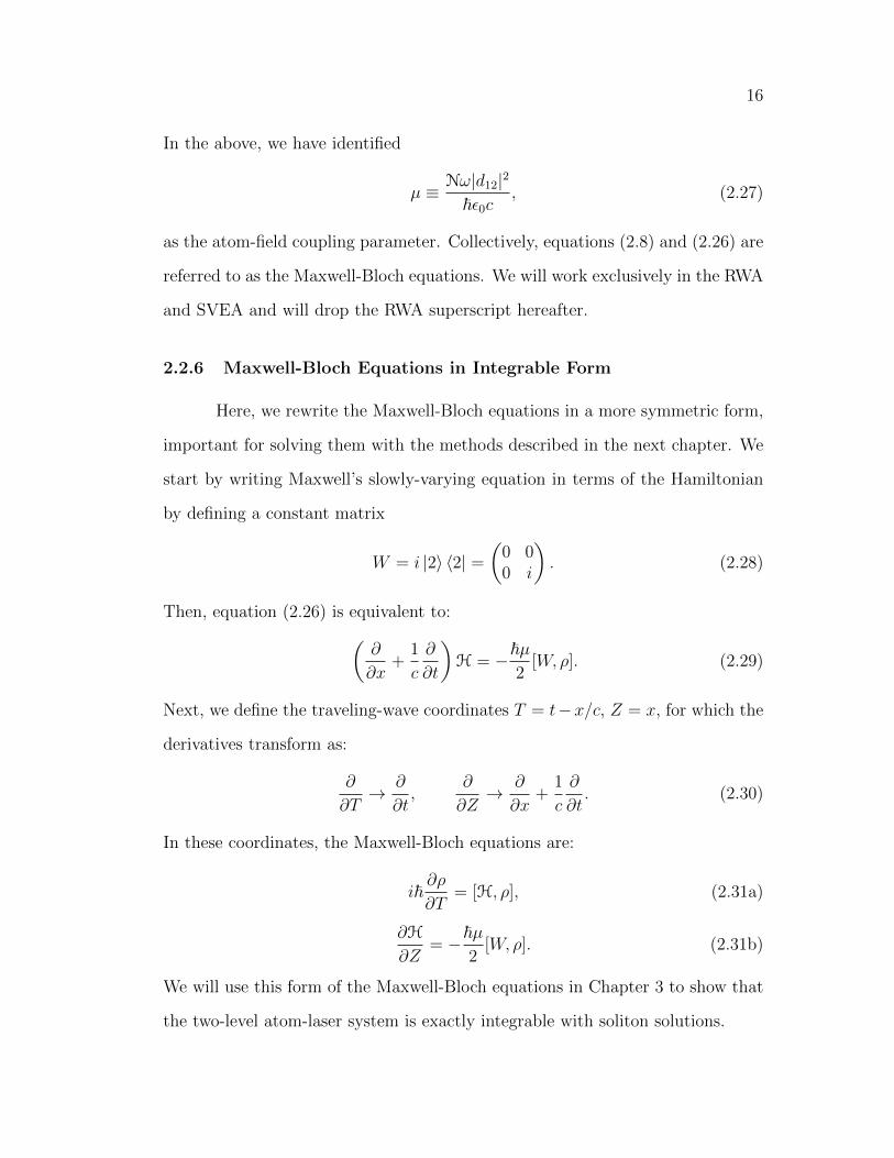
Figure 2.6: Theoretical model of a three-level atom. The signal pulse has fre-quency ω13 and drives transitions between levels 1 and 3 while the control pulsehas frequency ω23 and excites the 2-3 transition. The pulse frequencies may beslightly detuned from exact resonance, but we arrange the field frequencies toproduce equal detuning, ∆, for both. The atomic energies are ~ω1, ~ω2, and ~ω3

for levels 1, 2, 3, respectively. No decay channels are shown because they can beneglected in the short-pulse regime.

velopes.

The bare energy of the ith atomic state is ~ωi for i = 1, 2, 3. Each field

can be slightly detuned from the transition it addresses but we arrange equal

detunings for both: ∆ = ω3 − ω1 − ω13 = ω3 − ω2 − ω23. Thus, there is a double-

photon resonance even when there are no single-photon resonances. We assume

the transition between states 1 and 2 is dipole-forbidden due to the parity of the

levels, and the dipole moment operator is therefore:

~d = ~d13 |1〉 〈3|+ ~d23 |2〉 〈3|+ ~d31 |3〉 〈1|+ ~d32 |3〉 〈2| . (2.51)

As before, the particular values of the dipole moments depend on the atoms and

energy levels under consideration.

The system Hamiltonian is now 3x3:

H =

~ω1 0 −~d13 · ~E0 ~ω2 −~d23 · ~E

−~d31 · ~E −~d32 · ~E ~ω3

, (2.52)

26

where we have labelled the columns of the matrix in the energy eigenbasis:

|1〉 , |2〉 , |3〉 . The atomic evolution is characterized by the 3x3 density matrix:

ρ =

ρ11 ρ12 ρ13

ρ21 ρ22 ρ23

ρ31 ρ32 ρ33

, (2.53)

which evolves according to the von Neumann equation: i~∂ρ∂t

= [H, ρ].

As for the two-level atom, the diagonal elements of the density matrix

represent the atomic populations of their respective states and the off-diagonal

elements represent the coherence between them. The ground-state coherence,

ρ12, is particularly important for optical pulse control. The atom-laser system is

most conveniently characterized by the Rabi frequencies of the signal and control

pulses, Ω13(x, t) = 2~d13 ·~E13(x, t)/~ and Ω23(x, t) = 2~d23 ·~E23(x, t)/~, respectively.

2.3.1 Atomic Evolution in the RWA

We make the rotating wave approximation (RWA) as before, by transform-

ing into a rotating frame and neglecting fast oscillating terms. For the three-level

Λ-system, the unitary transformation that takes us to the rotating frame is:

U = eiω1t

1 0 00 e−i(k13x−ω13t)

0 0 e−i(k23x−ω23t)

. (2.54)

The Hamiltonian transforms as UHU † + i~∂U∂tU † and is therefore:

HRW = ~∆ |3〉 〈3|−(~d13 · ~E ei(k13x−ω13t) |1〉 〈3|+ ~d23 · ~E ei(k23x−ω23t) |2〉 〈3|+H.c.

),

in the rotating frame. The H.c. above stands for Hermitian conjugate. Using the

definition of the field in equation (2.50), we find that each off-diagonal element

has four terms.

In the rotating wave approximation, we discard the terms changing sign

too rapidly to have an appreciable effect on the system, including terms oscillating

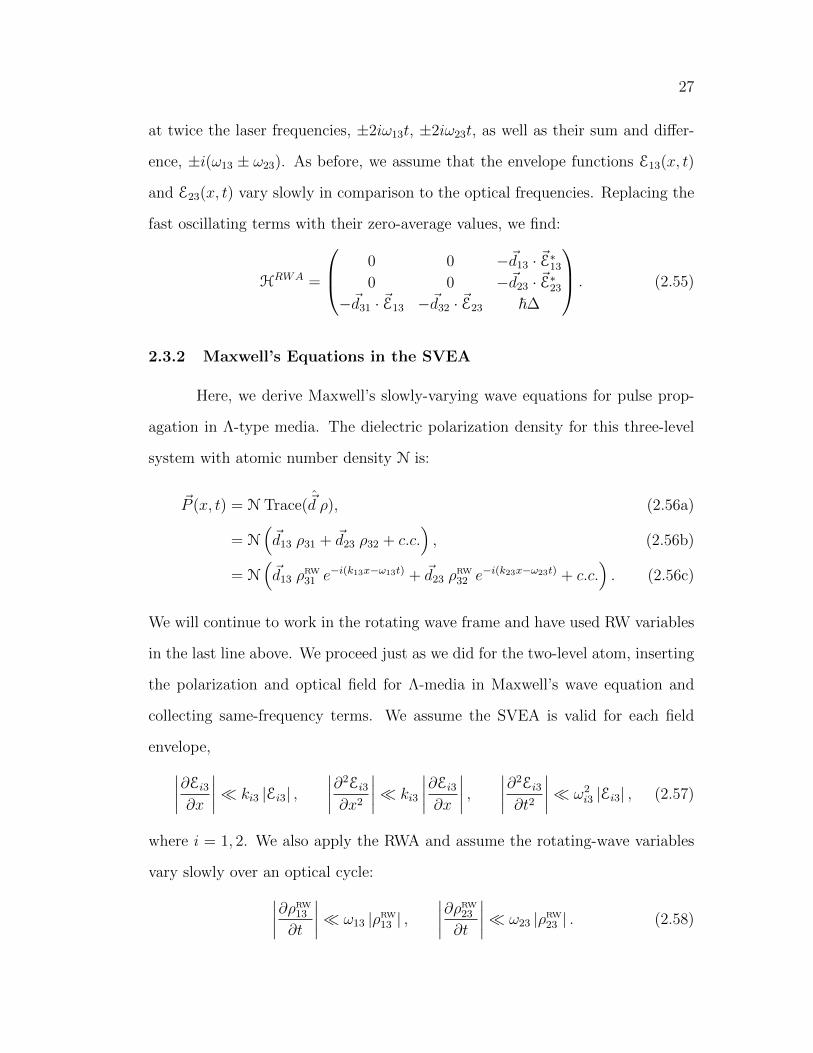
27

at twice the laser frequencies, ±2iω13t, ±2iω23t, as well as their sum and differ-

ence, ±i(ω13 ± ω23). As before, we assume that the envelope functions E13(x, t)

and E23(x, t) vary slowly in comparison to the optical frequencies. Replacing the

fast oscillating terms with their zero-average values, we find:

HRWA =

0 0 −~d13 · ~E∗13

0 0 −~d23 · ~E∗23

−~d31 · ~E13 −~d32 · ~E23 ~∆

. (2.55)

2.3.2 Maxwell’s Equations in the SVEA

Here, we derive Maxwell’s slowly-varying wave equations for pulse prop-

agation in Λ-type media. The dielectric polarization density for this three-level

system with atomic number density N is:

~P (x, t) = N Trace( ~d ρ), (2.56a)

= N(~d13 ρ31 + ~d23 ρ32 + c.c.

), (2.56b)

= N(~d13 ρ

RW

31 e−i(k13x−ω13t) + ~d23 ρ

RW

32 e−i(k23x−ω23t) + c.c.

). (2.56c)

We will continue to work in the rotating wave frame and have used RW variables

in the last line above. We proceed just as we did for the two-level atom, inserting

the polarization and optical field for Λ-media in Maxwell’s wave equation and

collecting same-frequency terms. We assume the SVEA is valid for each field

envelope,

∣∣∣∣∂Ei3∂x

∣∣∣∣ ki3 |Ei3| ,∣∣∣∣∂2Ei3

∂x2

∣∣∣∣ ki3

∣∣∣∣∂Ei3∂x

∣∣∣∣ ,∣∣∣∣∂2Ei3

∂t2

∣∣∣∣ ω2i3 |Ei3| , (2.57)

where i = 1, 2. We also apply the RWA and assume the rotating-wave variables

vary slowly over an optical cycle:

∣∣∣∣∂ρRW

13

∂t

∣∣∣∣ ω13 |ρRW

13 | ,∣∣∣∣∂ρRW

23

∂t

∣∣∣∣ ω23 |ρRW

23 | . (2.58)

28

These simplifications lead to a reduced wave equation for each field frequency:(∂

∂x+

1

c

∂

∂t

)Ω13 = iµ13 〈ρRW

31 〉 , (2.59a)

(∂

∂x+

1

c

∂

∂t

)Ω23 = iµ23 〈ρRW

32 〉 . (2.59b)

The brackets indicate an average over the detunings to account for Doppler broad-

ening, as in equation (2.40). The atom-field coupling constants (also referred to

as propagation constants) are µ13 ≡ Nω13|d13|2/~ε0c and µ23 ≡ Nω23|d23|2/~ε0c.

2.3.3 Maxwell-Bloch Equations in Integrable Form

We now rewrite the Maxwell-Bloch equations for three-level media in so-

called integrable form, which we will use to produce solutions in a later chapter.

When the atom-field coupling constants are equal, µ13 = µ23, the Maxwell-Bloch

equations can be written in this form and have soliton solutions. In the type

of atom-laser systems we model, the equal atom-field coupling approximation is

easily justified; using 87Rb atoms as an example, we shown the next section that

the coupling constants are equal to within 0.002%. We therefore define a generic

propagation constant µ ≡ µ13 = µ23, which enables us to write Maxwell’s slowly-

varying equations in terms of the Hamiltonian and a constant matrix, just as we

did for the two-level atom. If we define the constant matrix by:

W ≡ i |3〉 〈3| =

0 0 00 0 00 0 i

, (2.60)

then equations (2.59) can be combined into the single equation:(∂

∂x+

1

c

∂

∂t

)H = −~µ

2[W, ρ]. (2.61)

In the traveling-wave coordinates, T = t − x/c and Z = x, the Maxwell-

Bloch equations for Λ-type media are:

i~∂ρ

∂T= [H, ρ], (2.62a)

29

∂H

∂Z= −~µ

2[W, ρ], (2.62b)

where

H =

0 0 −~d13 · ~E∗13

0 0 −~d23 · ~E∗23

−~d31 · ~E13 −~d32 · ~E23 ~∆

. (2.62c)

Written in this way, we can see that the equations governing optical-pulse prop-

agation in Λ-type media are identical in form to the two-level single-pulse equa-

tions.

2.4 Real Atoms

The theoretical model we have derived applies to atoms with only two or

three accessible energy levels. Of course, no real atom has so few accessible states

and one might anticipate many complications to interfere with this simple model

in practice. Nevertheless, our model can been successfully applied to real atomic

systems under appropriate, limited, conditions. In this section, we calculate the

relevant parameters for coherent pulse propagation in a collection of 87Rb atoms.

The 87Rb D2 line is frequently used in experiments because its wavelength

(λ = 784 nm) is in the optical range and it has a cycling transition useful for laser

cooling and trapping [40]. Its relevant energy level splittings are shown in the

left panel of Figure 2.7; the data is taken from Steck [40]. As indicated in the left

panel of the figure, the D2 line connects the two fine-structure manifolds 52S1/2

(S = 1/2, L = 0, J = 1/2) and 52P3/2 (S=1/2, L=1, J=3/2). Each manifold

has hyperfine structure resulting from the coupling of the total electronic and

nuclear spins, labeled by the hyperfine quantum number F in the figure. Further

substructure is not shown, but each hyperfine state can be split in the presence

of a magnetic field via the Zeeman effect in the low-field limit. These splittings

30

Lifetime ~ 26 ns

4.27168 GHz

384.230 THz

52S1/2

52P3/2

72.2180 MHz

156.947 MHz

266.650 MHz

F = 1F = 0

F = 2

F = 3

2.56301 GHz

F = 1

F = 2

4.27168 GHz

6.83468 GHz

52S1/2

52P3/2

72.2180 MHz

156.947 MHz

266.650 MHz

F = 1F = 0

F = 2

F = 3

2.56301 GHz

F = 1

F = 2

4.27168 GHz

6.83468 GHz

384.230 THz

384.230THz + 4.27168 GHz

384.230 THz - 2.56005 GHz

52S1/2

52P3/2

72.2180 MHz

156.947 MHz

266.650 MHz

F = 1F = 0

F = 2

F = 3

2.56301 GHz

F = 1

F = 2

6.83468 GHz

Lifetime ~ 26 ns

87Rb D2 Line Transition

Two-Level Model

! < 2 ns

Large bandwidth pulse cannot resolve ground or excited hyperfine states

Three-Level Model

0.15 ns < ! < 2 ns

Pulse bandwidth chosen to resolve ground but not excited hyperfine states

Relevant Transition FrequenciesFocus on coherent effects by using laser pulses shorter than excited-state lifetime

! < 26 ns

Lifetime ~ 26 ns

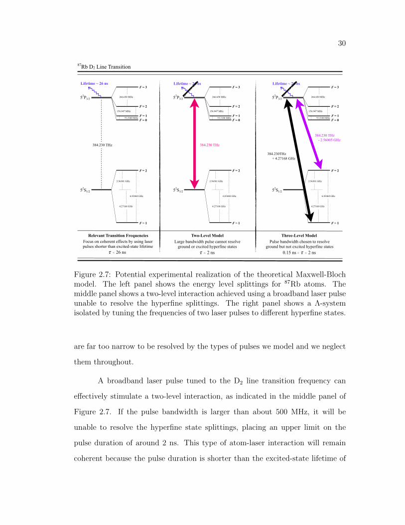
Figure 2.7: Potential experimental realization of the theoretical Maxwell-Blochmodel. The left panel shows the energy level splittings for 87Rb atoms. Themiddle panel shows a two-level interaction achieved using a broadband laser pulseunable to resolve the hyperfine splittings. The right panel shows a Λ-systemisolated by tuning the frequencies of two laser pulses to different hyperfine states.

are far too narrow to be resolved by the types of pulses we model and we neglect

them throughout.

A broadband laser pulse tuned to the D2 line transition frequency can

effectively stimulate a two-level interaction, as indicated in the middle panel of

Figure 2.7. If the pulse bandwidth is larger than about 500 MHz, it will be

unable to resolve the hyperfine state splittings, placing an upper limit on the

pulse duration of around 2 ns. This type of atom-laser interaction will remain

coherent because the pulse duration is shorter than the excited-state lifetime of

31

26 ns and can therefore be modeled by the Maxwell-Bloch equations previously

derived.

The theoretical model we derived for Λ-media can also be applied to 87Rb

atoms by exploiting the hyperfine structure of the ground-state manifold. As

indicated in the right panel of Figure 2.7, each laser frequency should be tuned

appropriately to address a single hyperfine ground state. To resolve the ground-

state splittings the pulse bandwidths must be less than about 6.8 GHz, placing a

lower limit on the pulse durations of about 0.15 ns. As we assumed for our the-

oretical model, transition between the ground states is dipole forbidden because

the dipole operator only couples states of opposite parity (∆L = ±1).

The transition dipole moments can be calculated for each model [40] and

for a linearly polarized field the effective dipole moment is:

|deff|2 ≈1

3|4.2275ea0|2 ≈ 6|ea0|2 ≈

1

3|3.5842× 10−29|2C ·m2, (2.63)

where e is the electron charge and a0 is the Bohr radius. The dipole moment cal-

culated above is independent of the hyperfine ground state and is therefore appli-

cable to the two-level atom model and either of the pulses in the Λ-configuration.

Recall that the atom-field coupling parameter from Maxwell’s slowly-varying

equation is:

µ = Nω|deff|2/~ε0c. (2.64)

The atom-field coupling parameters differ only by the transition frequencies be-

cause the dipole moments are identical for each transition. When modeling two

pulses in the Λ-configuration of 87Rb atoms, one can therefore take µ13 ≈ µ23 to

within an accuracy of 0.002%.

32

Chapter 3

An Introduction to Integrable Systems

It has long been established that the equations governing the coherent

propagation of optical fields through resonant nonlinear media permit soliton so-

lutions. As we explained, in the simplest non-trivial soliton solution, a hyperbolic

secant pulse of 2π-area induces absorption and stimulated emission of the atoms

in such a way that the pulse travels without a change in shape or area, but with

a group velocity which may be much slower than the speed of light. This phe-

nomenon was given the name of Self-Induced Transparency (SIT) by McCall and

Hahn who were the first to observe it experimentally [38, 39]. Many sophisti-

cated techniques of producing the exact solution have since been employed [28].

In particular, the Backlund Transformation was discovered in the early 1800s to

connect solutions of the Sine-Gordon equation (2.39) and later applied by Lamb

[41] to the coherent pulse propagation problem to produce the SIT solution.

The Backlund Transformation used by Lamb is straightforward to use

but is of limited applicability. The Sine-Gordon equation applies to coherent

pulse propagation only when the field Rabi frequency is real and the medium is

composed of two-level atoms in a pure state. A more general transformation was

produced by Park and Shin [42] and then further extended by them to apply to

two-pulse, three-level systems in the lambda configuration [43, 44]. Park and Shin

derived their method using a matrix potential that exploited a gauge invariance

in the system. The reformulation of this method by Clader and Eberly [45]

moved away from the matrix potential and increased the transparency of the

33

method. In this chapter, we provide the background necessary to understand

their introduction of a projection operator and the form of their transformation

by reviewing the framework implicit in their derivation.

There are many sophisticated methods of producing soliton solutions to

nonlinear equations, including Inverse Scattering [37], the dressing method of

Zakharov and Shabat [28], the direct method of Hirota [46], as well as Backlund

and Darboux transformations [28]. Any nonlinear partial differential equation

solvable by these techniques arises as the integrability condition of an overdeter-

mined set of linear partial differential equations. These nonlinear equations are

therefore said to be integrable and can be described by the Lax formalism. In

this section, we will define the Lax formalism and introduce the so-called Lax

operators in order to show how they can be used to define a Backlund-Darboux

(or simply Darboux) transformation matrix. Once this transformation matrix is

known, complicated solutions can be generated in a remarkably straightforward

way; in general, constructing the transformation matrix is the challenge. Here,

we demonstrate that for a limited set of nonlinear partial differential equations

the Backlund-Darboux transformation can be generated in an algorithmic way.

This chapter contains a detailed analysis of the origin of the solution

method we will use throughout. Our aim in such a thorough derivation is to

highlight how the method fits into the broader subject of integrable and nonlinear

systems. Arming ourselves with these details will, we hope, enable application of

the method to new multi-pulse systems in future work.

34

3.1 Lax Formalism

As a simple example to motivate the Lax formalism, consider the linear

partial differential matrix equations [28]:

∂xΨ =

(λ u−u −λ

)Ψ ≡ UΨ (3.1a)

∂tΨ =

(−4λ3 − 2λu2 −4λ2u− 2λ∂xu− 2u3 − ∂xxu

4λ2u− 2λ∂xu+ 2u3 + ∂xxu 4λ3 + 2λu2

)Ψ (3.1b)

≡ VΨ

where u is a scalar function of x and t, λ is a constant, and we use the shorthand

∂x ≡ ∂/∂x and similarly for the other partial differentials. For convenience, we

have defined the matrices U and V as shown. This set of matrix equations is

overdetermined because for a given operator Ψ there are two equations that the

unspecified function u must satisfy.

That is, both equations will not be satisfied for an arbitrary function u. In

order to ensure that these two matrix equations are compatible, it must be true

that if we calculate ∂xtΨ from the first equation and ∂txΨ from the second, that

they are exactly equal. From the time derivative of equation (3.1a), we have:

∂xtΨ = (∂tU)Ψ + U∂tΨ = (∂tU)Ψ + UVΨ, (3.2)

where we have used equation (3.1b) for the time derivative of Ψ in the last step.

Similarly, by taking the spatial derivative of equation (3.1b) we find:

∂txΨ = (∂xV )Ψ + V ∂xΨ = (∂xV )Ψ + V UΨ. (3.3)

Insisting on integrablity or compatibility, that ∂xtΨ = ∂txΨ, thus requires:

∂tU − ∂xV + [U, V ] = 0, (3.4)

35

which is known as the Lax equation. In terms of the unspecified function u, the

Lax equation reads:

∂tu+ 6u2∂xu+ ∂xxxu = 0. (3.5)

Equation (3.5) is the Modified Korteweg-de-Vries (MKdV) equation, which is

a nonlinear partial differential equation that has been used to study plasmas

and fluid mechanics [47, 48]. We have therefore found that the nonlinear MKdV

equation is the integrability condition for the associated linear system in equation

(3.1). The MKdV equation is thus often said to describe an integrable system.

Many nonlinear partial differential equations, including the Sine-Gordon,

KdV, and nonlinear Schrodinger equations to name a few [28], can be written

in Lax form, as in equation (3.4). The so-called Lax operators U ≡ U(x, t, λ)

and V ≡ V (x, t, λ) depend on space and time in addition to a complex constant,

λ, referred to as the spectral parameter. In the above, we have restricted the

discussion to a system described by only two independent variables, x and t,

but the Lax formalism can be extended to describe more complicated systems

dependent on any number of variables (x, y, z, and t, for example) as well as a

non-constant spectral parameter [33]. When λ is constant the problem is said to

be isospectral and we will assume this is the case throughout.

We have seen that the Lax equation is a compatibility or integrability

condition of the overdetermined linear system:

∂xΨ = UΨ, (3.6a)

∂tΨ = VΨ, (3.6b)

for the so-called fundamental solution Ψ ≡ Ψ(x, t, λ). Any nonlinear equation

that can be written in Lax form arises as the integrability condition of its asso-

ciated linear system and is called an integrable equation or system.

36

3.1.1 Connecting Soliton Solutions

Having classified the types of nonlinear equations we are interested in

solving, we now show how to exploit the Lax formalism to construct new solutions.

Suppose we make a gauge-like transformation

Ψ ≡ DΨ, (3.7)

using some invertible matrix operator D ≡ D(x, t, λ), to be determined. Then,

using equation (3.6) one can show that:

∂xΨ = U Ψ, (3.8a)

∂tΨ = V Ψ, (3.8b)

where

U = DUD−1 + (∂xD)D−1, (3.9a)

V = DVD−1 + (∂tD)D−1. (3.9b)

Given a solution to an integrable nonlinear equation (a known solution u of the

MKdV equation, for example), we can find the Lax operators U and V from

their definition with respect to u and then solve equation (3.6) to obtain Ψ.

The transformation matrix D connects this known solution to the transformed

operators Ψ, U, V , which we see from equation (3.8) are also solutions to the

linear Lax equation. One thus has a new solution to the nonlinear evolution

equation, u from the definition of the Lax operators. In the case of the MKdV

equation, the off-diagonal component of the Lax operator U is exactly equal to

the nonlinear solution u and the new solution u is thus easily found once U is

known.

37

This simple way of connecting solutions is only useful if the Darboux ma-

trix is constructed in terms of some known quantities. When the transformation

matrix is constructed from the original solution Ψ and the original and trans-

formed Lax operators have the same spectral dependence (that is, poles and

zeroes of λ and their multiplicities), the transformation matrix D is called a Dar-

boux matrix and the linear equations are said to be Darboux covariant [33]. We

will show how to find the explicit form of the Darboux matrix for a limited set

of Lax operators in the next section.

3.1.2 Constructing a Darboux Transformation

Many methods of constructing a Darboux transformation exist, many of

which are equivalent [28, 33]. The important points to consider are that the

transformation matrix must be constructed in terms of the original solution of the

linear equation, Ψ, and that the spectral dependence of the Darboux matrix must

be chosen in a way that will preserve the spectral form of the Lax pair. A great

advantage of the Darboux matrix is that it can be constructed algorithmically.

The general idea is to choose how D depends on the spectral parameter and then

derive a series of conditions D must satisfy so that the transformed Lax operators

have the same spectral dependence as the original.

For simplicity and concreteness, we will focus on Lax pairs with the specific

spectral dependence:

U(x, t, λ) ≡ λ−1U−1(x, t) + U0(x, t) + λU1(x, t), (3.10a)

V (x, t, λ) ≡ λ−1V−1(x, t) + V0(x, t) + λV1(x, t), (3.10b)

and we will further suppose that the Darboux matrix is a rational function of λ

with only a single simple pole. Such a transformation matrix is usually referred

38

to as either the “Backlund-Darboux” [33] or the “1-soliton” Darboux matrix [31].

We follow much of the procedure for its construction as outlined by Cieslinski,

[31]. If we insist that the inverse of the Darboux matrix is also a rational function

of λ with one simple pole, then one can show that the Darboux matrix must be

of the form:

D = N

(I +

(λ1 − µ1

λ− λ1

)P

), (3.11)

where the matrix P is a projection operator, i.e. P 2 = P , or alternatively:

D = N

(I +

(µ1

λ− λ1

)S

), (3.12)

where the matrix S is nilpotent, i.e. S2 = 0. In the above, the matrices N,P, S

must be independent of the spectral parameter λ and N must be invertible. The

parameters λ1 and µ1 are complex constants often referred to as Backlund or

Darboux parameters. Additional constraints on N and either P or S are obtained

by requiring that the transformed Lax pair has the same spectral dependence as U

and V in equation (3.10). For many systems, there remains freedom in the choice

of the so-called “normalization” matrix N and its components can be chosen to

simplify the overall appearance of the Darboux matrix. Such is the case for the

Lax operators we are interested in and we will take N = I.

The choice of whether to use the first or second form of the Darboux

matrix is arbitrary, but the first form is more commonly used and we therefore

proceed with it. Note that U and V are insensitive to changes in the Darboux

matrix up to an overall (invertible) function of λ. That is, if D → f(λ)D then

U → U and V → V and the Darboux matrices are said to be Darboux equivalent.

For simplicity in later sections we will choose f(λ) = λ− λ1. Thus, our Darboux

matrix is of the form:

D = (λ− λ1)I + (λ1 − µ1)P, (3.13)

39

and we will determine the projection operator explicitly in a later section.

3.1.3 Unitary Reduction

We have already noted that the Darboux method preserves the spectral

dependence of the Lax pair. In addition, it may be desirable for other properties

to be preserved under the Darboux transformation. For example, the Hamilto-

nian and density matrix of the Maxwell-Bloch system are Hermitian and, for a

particular choice of their associated Lax pair, this requires that:

U(λ)† = −U(λ∗), (3.14a)

V (λ)† = −V (λ∗). (3.14b)

The star and dagger denote complex and Hermitian conjugation, respectively,

above. Lax operators with this property belong to the so-called unitary reduc-

tion. To ensure that the transformed Lax pair maintain the property in equation

(3.14) after Darboux transformation, one must impose further constraints on the

Darboux matrix. One can show that the unitary reduction will be preserved if

µ1 = λ∗1 and P = P † in equation (3.13) above (see [31] for a proof). With these

choices, the Darboux matrix is:

D = (λ− λ1)I + (λ1 − λ∗1)P. (3.15)

and is said to be written in “elementary form”.

A complex Darboux parameter λ1 with non-zero real and imaginary parts

leads to more complicated types of solutions than we will pursue in later sections.

Hereafter, we will suppose the Darboux parameter has no real part, λ1 = −λ∗1.

Then, the Darboux matrix takes the simple form:

D = λI + λ1(2P − I). (3.16)

40

We note that our definition of the Darboux matrix differs from that of Clader

and Eberly [45] only by a factor of λ. The transformation matrices are therefore

Darboux equivalent and all final results will be the same.

3.1.4 Explicit Form of the Darboux Matrix

We now construct the explicit form of the Darboux matrix in order to

understand what determines the projection operator P as well as the Darboux

parameter λ1. Darboux covariant Lax operators have the same spectral depen-

dence before and after the transformation and we can therefore use the notation:

U(x, t, λ) ≡ λ−1U−1(x, t) + U0(x, t) + λU1(x, t), (3.17a)

V (x, t, λ) ≡ λ−1V−1(x, t) + V0(x, t) + λV1(x, t). (3.17b)

On the other hand, by definition of the transformed Lax operators, we have:

UD = DU + ∂xD, (3.18a)

V D = DV + ∂tD. (3.18b)

Plugging into the above our chosen form of the Darboux matrix from equation

(3.16), as well as the original and transformed Lax pairs, (equation (3.10) and

equation (3.17), respectively), and collecting like orders of λ, we find:

λ−1 : U−1M = MU−1, (3.19a)

λ0 : U−1 + λ1U0M = U−1 + λ1MU0 + λ1∂xM, (3.19b)

λ1 : U0 + λ1U1M = U0 + λ1MU1, (3.19c)

λ2 : U1 = U1. (3.19d)

We have introduced the Hermitian unitary matrix operator M ≡ 2P − I in the

above to simplify the notation.

41

A similar set of conditions can be derived for Lax operator V with the

partial derivative with respect to space replaced with one with respect to time:

λ−1 : V −1M = MV−1, (3.20a)

λ0 : V −1 + λ1V 0M = V−1 + λ1MV0 + λ1∂tM, (3.20b)

λ1 : V 0 + λ1V 1M = V0 + λ1MV1, (3.20c)

λ2 : V 1 = V1. (3.20d)

We will use these equations to show how to construct the projection operator

from the original solution.

First, we insert U1 = U1 from equation (3.19d) in equation (3.19c) to find:

U0 = U0 + λ1MU1 − λ1U1M. (3.21)

Next, solving for U−1 in equation (3.19a) and putting the result into equation

(3.19b), one finds:

MU−1M = U−1 − λ1U0M + λ1MU0 + λ1∂xM. (3.22)

Rearranging and using equation (3.21) yields:

λ1∂xM + U−1 −MU−1M + λ1MU0 − λ1U0M + λ21U1 − λ2

1MU1M = 0, (3.23)

In the above, we have used the fact that M is an involution, i.e. M2 = I, since P

is a projection operator. We can simplify this equation by multiplying through

on the left with M − I and noting that (M − I)M = −(M − I). The result is:

(M − I)(λ1∂xM + U−1 + U−1M − λ1U0 − λ1U0M+

λ21U1 + λ2

1U1M) = 0, (3.24)

or, rearranging:

(M − I)(λ1∂xM + U−1(I +M)− λ1U0(I +M) + λ2

1U1(I +M))

= 0. (3.25)

42

Finally, we find

(M − I)

(I∂

∂x+ λ−1

1 U−1 − U0 + λ1U1

)(M + I) = 0. (3.26)

In terms of the projection operator, we finally find:

(P − I)

(I∂

∂x− U(−λ1)

)P = 0, (3.27)

where we have identified U(−λ1) = −λ−11 U−1+U0−λ1U1. One often sees equation

(3.27) written in terms of U(λ∗1) rather than U(−λ1). Note that in our case

U(λ∗1) = U(−λ1), since we have previously assumed that the Darboux parameter

is purely imaginary. Similarly, one can show that equation (3.20) implies that:

V 0 = V0 + λ1MU1 − λ1V1M (3.28)

and

(P − I)

(I∂

∂t− V (−λ1)

)P = 0. (3.29)

Finally, then, we have derived equations for the projection operator P in terms

of the original known solution to the Lax equations.

To solve, we note that since P is a Hermitian projection operator, it can

be written P = |φ〉〈φ|〈φ|φ〉 , where the so-called wavefunction |φ〉 is an n-dimensional

column vector. Equation (3.27) is satisfied for any eigenvalue a of the operator

I ∂∂x− U(−λ1) with associated eigenvector |φ〉. That is, if

(I∂

∂x− U(−λ1)

)|φ〉 = a |φ〉 , (3.30)

then

(P − I)

(I∂

∂x− U(−λ1)

)P = a(P − I)P = 0, (3.31)

since P is a projection operator. Similarly, if

(I∂

∂t− V (−λ1)

)|φ〉 = b |φ〉 (3.32)

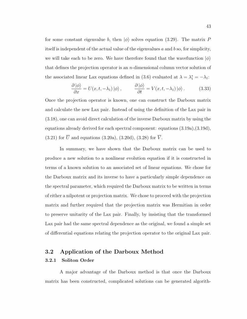
43

for some constant eigenvalue b, then |φ〉 solves equation (3.29). The matrix P

itself is independent of the actual value of the eigenvalues a and b so, for simplicity,

we will take each to be zero. We have therefore found that the wavefunction |φ〉

that defines the projection operator is an n-dimensional column vector solution of

the associated linear Lax equations defined in (3.6) evaluated at λ = λ∗1 = −λ1:

∂ |φ〉∂x

= U(x, t,−λ1) |φ〉 , ∂ |φ〉∂t

= V (x, t,−λ1) |φ〉 . (3.33)

Once the projection operator is known, one can construct the Darboux matrix

and calculate the new Lax pair. Instead of using the definition of the Lax pair in

(3.18), one can avoid direct calculation of the inverse Darboux matrix by using the

equations already derived for each spectral component: equations (3.19a),(3.19d),

(3.21) for U and equations (3.20a), (3.20d), (3.28) for V .

In summary, we have shown that the Darboux matrix can be used to

produce a new solution to a nonlinear evolution equation if it is constructed in

terms of a known solution to an associated set of linear equations. We chose for

the Darboux matrix and its inverse to have a particularly simple dependence on

the spectral parameter, which required the Darboux matrix to be written in terms

of either a nilpotent or projection matrix. We chose to proceed with the projection

matrix and further required that the projection matrix was Hermitian in order

to preserve unitarity of the Lax pair. Finally, by insisting that the transformed

Lax pair had the same spectral dependence as the original, we found a simple set

of differential equations relating the projection operator to the original Lax pair.

3.2 Application of the Darboux Method

3.2.1 Soliton Order

A major advantage of the Darboux method is that once the Darboux

matrix has been constructed, complicated solutions can be generated algorith-

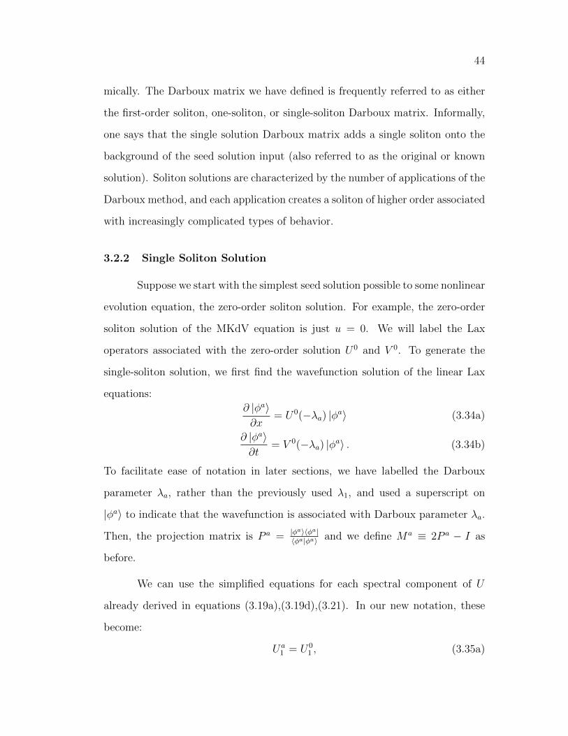
44

mically. The Darboux matrix we have defined is frequently referred to as either

the first-order soliton, one-soliton, or single-soliton Darboux matrix. Informally,

one says that the single solution Darboux matrix adds a single soliton onto the

background of the seed solution input (also referred to as the original or known

solution). Soliton solutions are characterized by the number of applications of the

Darboux method, and each application creates a soliton of higher order associated

with increasingly complicated types of behavior.

3.2.2 Single Soliton Solution

Suppose we start with the simplest seed solution possible to some nonlinear

evolution equation, the zero-order soliton solution. For example, the zero-order

soliton solution of the MKdV equation is just u = 0. We will label the Lax

operators associated with the zero-order solution U0 and V 0. To generate the

single-soliton solution, we first find the wavefunction solution of the linear Lax

equations:

∂ |φa〉∂x

= U0(−λa) |φa〉 (3.34a)

∂ |φa〉∂t

= V 0(−λa) |φa〉 . (3.34b)

To facilitate ease of notation in later sections, we have labelled the Darboux

parameter λa, rather than the previously used λ1, and used a superscript on

|φa〉 to indicate that the wavefunction is associated with Darboux parameter λa.

Then, the projection matrix is P a = |φa〉〈φa|〈φa|φa〉 and we define Ma ≡ 2P a − I as

before.

We can use the simplified equations for each spectral component of U

already derived in equations (3.19a),(3.19d),(3.21). In our new notation, these

become:

Ua1 = U0

1 , (3.35a)

45

Ua−1 = MaU0

−1Ma, (3.35b)

Ua0 = U0

0 + λaMaU0

1 − λaU01M

a, (3.35c)

where Ua = λ−1Ua−1+Ua+λUa

1 and the zero-order seed is U0 = λ−1U0−1+U0

0 +λU01 .

Similar equations are satisfied by the components of the Lax operator V a =

λ−1V 0−1 + V 0

0 + λV 01 :

V a1 = V 0

1 , (3.36a)

V a−1 = MaV 0

−1Ma, (3.36b)

V a0 = V 0

0 + λaMaV 0

1 − λaV 01 M

a, (3.36c)

where V 0 = λ−1V 0−1 + V 0

0 + λV 01 .

3.2.3 Double Soliton Solution

Once we have derived a first-order soliton solution, we can use it as the seed

solution to generate a second-order soliton (also referred to as a double-soliton or

two-soliton solution). In describing the method, we will label the operators of the

second-order solution with an ab superscript to indicate that we generated the

single-soliton seed with Darboux parameter λa and will use a different Darboux

parameter λb 6= λa in the second application of the Darboux matrix (see Figure

3.1).

To find the double-soliton solution, we must find the new wavefunction

|φab〉 by solving the linear Lax equations with seed Ua, V a evaluated at λ = −λb:

∂ |φab〉∂x

= Ua(−λb) |φab〉 , (3.37a)

∂ |φab〉∂t

= V a(−λb) |φab〉 . (3.37b)

46

Zero-order soliton U0, V 0

First-order soliton Ua, V a

λa Da = λI + λaMa

?

Second-order soliton Uab, V ab

λb Dab = λI + λbMab

?

Figure 3.1: Method of producing a second-order soliton solution. The single-soliton is first produced from the zero-order soliton and subsequently used as aseed solution in constructing the second-order soliton solution.

Once |φab〉 is known, we define P ab = |φab〉〈φab|〈φab|φab〉 and Mab = 2P ab− I as usual. The

equations for the second-order Lax operator Uab = λ−1Uab−1 +Uab

0 +λUab1 are then:

Uab1 = Ua

1 = U01 , (3.38a)

Uab−1 = MabUa

−1Mab = MabMaU0

−1MaMab (3.38b)

Uab0 = Ua

0 + λb[Mab, Ua

1 ] = U00 + [λaM

a + λbMab, U0

1 ] (3.38c)

where we have used equation (3.35) in the last steps.

3.2.4 Nonlinear Superposition Rule

Although the method for producing higher-order solitons does not change,

calculating the projection operator becomes increasingly difficult as the seed so-

lutions become more complicated. Solving the linear differential equations with

a non-trivial seed solution (as in equation (3.37), for example) can be extremely

challenging. Fortunately, we can construct a so-called Theorem of Permutability

[28] that is a nonlinear superposition rule that combines two nth-order solitons

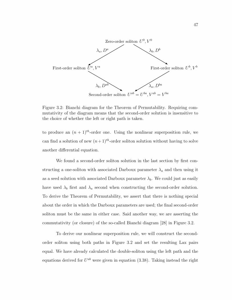
47

Zero-order soliton U0, V 0

First-order soliton Ua, V a

λa, Da

First-order soliton U b, V b

λb, Db

-

Second-order soliton Uab = U ba, V ab = V ba

λa, Dba

λb, D

ab

-

Figure 3.2: Bianchi diagram for the Theorem of Permutability. Requiring com-mutativity of the diagram means that the second-order solution is insensitive tothe choice of whether the left or right path is taken.

to produce an (n + 1)th-order one. Using the nonlinear superposition rule, we

can find a solution of new (n+ 1)th-order soliton solution without having to solve

another differential equation.

We found a second-order soliton solution in the last section by first con-

structing a one-soliton with associated Darboux parameter λa and then using it

as a seed solution with associated Darboux parameter λb. We could just as easily

have used λb first and λa second when constructing the second-order solution.

To derive the Theorem of Permutability, we assert that there is nothing special

about the order in which the Darboux parameters are used; the final second-order

soliton must be the same in either case. Said another way, we are asserting the

commutativity (or closure) of the so-called Bianchi diagram [28] in Figure 3.2.

To derive our nonlinear superposition rule, we will construct the second-

order soliton using both paths in Figure 3.2 and set the resulting Lax pairs

equal. We have already calculated the double-soliton using the left path and the

equations derived for Uab were given in equation (3.38). Taking instead the right

48

path and following the procedure used in the last section, one finds:

U ba1 = U b

1 = U01 , (3.39a)

U ba−1 = M baU b

−1Mba = M baM bU0

−1MbM ba (3.39b)

U ba0 = U b

0 + λa[Mba, U b

1 ] = U00 + [λbM

b + λaMba, U0

1 ] (3.39c)

Equating Uab−1 and U ba

−1, we find a relationship between the various unitary ma-

trices:

MabMaU−1MaMab = M baM bU−1M

bM ba, (3.40a)

⇒MabMaU−1(MabMa)−1 = M baM bU−1(M baM b)−1, (3.40b)

⇒MabMa = M baM b. (3.40c)

To eliminate the explicit appearance of the Lax operators and find an expression

for Mab in terms of just the single-soliton unitary operators, we set Uab0 from

equation (3.38c) equal to U ba0 from equation (3.39c). The result is:

λbMb + λaM

ba = λaMa + λbM

ab. (3.41a)

Using the relationship between Mab and M ba found in equation (3.40c),

we find:

λbMb + λaM

abMaM b = λaMa + λbM

ab, (3.41b)

or, rearranging,

Mab = (λaMa − λbM b)(λaM

aM b − λbI)−1. (3.41c)

This remarkable result says that we can calculate the second-order unitary op-

erator Mab from the single-soliton operators Ma and M b using simple algebraic

methods; no complicated differential equations need to be solved. Once Mab is

known, the Lax operator Uab is immediately determined from equation (3.38).

49

We will demonstrate this powerful method of constructing a two-soliton solution

for the Maxwell-Bloch system in a later section. First, we must show that the

Maxwell-Bloch system supports soliton solutions.

50

Chapter 4

Soliton Solutions for Two-Level Media

We have described how to produce exact soliton solutions to particular

types of nonlinear evolution equations. Now, we apply our developed formalism

to atom-laser systems commonly used in quantum optics experiments. We now

reap the benefits of having carefully derived the solution method in the last

chapter, as we will be able to derive complicated soliton solutions systematically

using mostly algebraic techniques.

To start, we produce a first-order soliton solution for a single optical pulse

propagating in a medium with two accessible energy states: the 2π-area Self-

Induced Transparency solution previously described. We then nonlinearly super-

impose two of these solutions to derive a second-order two-pulse soliton solution

and demonstrate the properties of soliton collision in this relatively simple sys-

tem. We will pay special attention to the integration constants and the Darboux

parameter in these soliton solutions in preparation for understanding the more

complicated and important role they play in the three-level solutions we derive

in the next chapter.

4.1 Lax Operators

To show that the Maxwell-Bloch equations are integrable, we will identify

their associated Lax pair and show that they can be combined and written in

51

Lax form [27]:

∂U

∂t− ∂V

∂x+ [U, V ] = 0, (4.1)

where the Lax operators U and V are some combination of the density matrix

and Hamiltonian of the system. There are several ways to arrive at the Lax

equation, each resulting in slightly different Lax operators. We start by taking

what is perhaps the most direct route by rewriting the von Neumann equation

and the matrix form of Maxwell’s slowly-varying equation (in equation (2.31))

more symmetrically, as in:

∂Tρ+ [ρ,− i~H] = 0, (4.2)

and

∂Z

(− i~H

)+ [ρ,

iµ

2W ] = 0, (4.3)

respectively. We then combine these two matrix equations by multiplying equa-

tion (4.2) by an arbitrary constant, λ, and subtracting it from equation (4.3).

After some simple rearranging, we find:

∂Z

(− i~H

)− λ∂Tρ+ [− i

~H − iµ

2λW, λρ] = 0 (4.4)

We introduced the arbitrary constant λ (which must have units of inverse dis-

tance) to allow us to separate the single equation back into the original two.

We can recognize the formula above as the Lax equation by identifying: λ

as the spectral parameter, the coordinates x = T, t = Z, and the Lax operators:

U = − i~H − iµ

2λW, (4.5a)

V = λρ, (4.5b)

By writing the Maxwell-Bloch equations in Lax form, we have shown that these

nonlinear evolution equations are integrable and can be solved with the methods

reviewed in the previous chapter.

52

Although the Lax operators above arose in a fairly natural way, we will

proceed instead with the Lax pair identified by Clader and Eberly [45] for conti-

nuity with their work:

U = − i~H − λW, (4.6a)

V =iµ

2λρ. (4.6b)

For this choice of Lax operators, the spectral parameter has units of inverse time.

One can easily check that the Lax equation exactly produces the von Neumann

and slowly-varying Maxwell equations for these Lax operators by: plugging in

U and V explicitly, identifying x = T, t = Z, and collecting like orders of the

spectral parameter.

4.2 First-Order Soliton Solution

The density matrix and Hamiltonian of any solution to the Maxwell-Bloch

equations must be Hermitian. In terms of the Lax operators in equation (4.6),

this implies that:

U(λ)† = −U(λ∗), and V (λ)† = −V (λ∗). (4.7)

The Maxwell-Bloch system therefore belongs in the unitary reduction identified

in Section 3.1.3. The transformation equations we derived in that section pre-

serve unitarity of the Lax operators and will therefore preserve Hermiticity of the

density matrix and Hamiltonian of connected solutions. In the notation of that

chapter, the Maxwell-Bloch Lax operators were written:

U = λ−1U−1 + U0 + λU1, (4.8a)

V = λ−1V−1 + V0 + λV1. (4.8b)

53

The corresponding terms for the Lax operators of the Maxwell-Bloch system are:

U−1 = 0, U0 = − i~H, U1 = −W, (4.9a)

V−1 =iµ

2ρ, V0 = 0, V1 = 0. (4.9b)

We can insert these definitions into equations (3.35) and (3.36) to connect a

known, zero-order seed solution of the Maxwell-Bloch equations associated with

Darboux parameter λ0 to a new, first-order soliton solution associated with Dar-

boux parameter λa.

Notice that equations (3.35a) and (3.36a) indicate that the terms linear

in the spectral parameter of the Lax operators stay the same between solutions.

That is, Ua1 = U0

1 and therefore the constant matrix does not change: W 0 =

W a = W . Using this result in equation (3.35c), we find a relationship between

the Hamiltonia of the zero-order and first-order soliton solutions:

Ha = H0 − i~λa[Ma,W ]. (4.10)

Recall that the unitary matrix is defined by: Ma = 2P a − I, where P a is the

projection operator,

P a =|φa〉 〈φa|〈φa|φa〉 , (4.11)

and the wavefunction |φa〉 is the solution to the linear Lax equations evaluated

at λ = −λa:

∂ |φa〉∂T

= U0(−λa) |φa〉 =

(− i~H0 + λaW

)|φa〉 , (4.12a)

∂ |φa〉∂Z

= V 0(−λa) |φa〉 =

(− iµ

2λaρ0

)|φa〉 . (4.12b)

Evaluating the commutator in equation (4.10), one finds:

Ha = H0 + ~λa(

0 Ma12

−Ma∗12 0

). (4.13)

54

We therefore find a simple formula for the first-order soliton pulse Rabi frequency:

Ωa12 = Ω0

12 + 2λaMa∗

12 . (4.14)

Inserting the Maxwell-Bloch operator V in equation (3.36b) gives the re-

lationship between the density matrices of the zero-order and first-order soliton

solutions:

ρa = Maρ0Ma. (4.15)

Given any seed solution, we can now use it to compute a first-order one-pulse

soliton solution.

We use a zero-order seed solution with zero detuning, for which all of the

atoms are in the ground state ρ11 = |1〉 〈1| and the laser field is “off” so that the

field envelope is identically zero: E = 0. The associated Lax operators are:

U0 = − i~H0 − λ0W = −λ0

(0 00 i

), (4.16a)

V 0 =iµ

2λ0

ρ0 =iµ

2λ0

(1 00 0

). (4.16b)

The wavefunction |φa〉 is found by solving the linear Lax equations (4.12). We

find:

|φa〉 = exp

[− iµ

2λaZ

(1 00 0

)+ λaT

(0 00 i

)](a1

a2

), (4.17)

=

(a1e−iµZ/2λa

a2eiλaT

), (4.18)

where a1 and a2 are constants of integration. Recall that we chose λa = −λ∗a in

Section 3.1.3 and so the off-diagonal element of the unitary matrix operator is:

Ma12 = 2P a

12 =2a1a

∗2eiλaT−µZ/2λa

|a1a2|(e−iµZ/2λa+ηa12 + e2iλaT−ηa12

) , (4.19)

=a1a

∗2

|a1a2|sech (−iµZ/2λa − iλaT + ηa12) . (4.20)

55

In the above, we have defined ηa12 ≡ ln |a1/a2| to simplify the notation.

The pulse Rabi frequency can now be calculating using equation (4.14)

and we find:

Ωa12 =

2λaa∗1a2

|a1a2|sech(−iµZ/2λa − iλaT + ηa12). (4.21)

We have therefore shown that the first-order one-pulse soliton pulse Rabi fre-

quency is a traveling hyperbolic secant with temporal pulse width, or duration,

characterized by the Darboux parameter. It is natural, then, to define the real

and positive “pulse duration” τa through λa ≡ i/τa. To simplify the notation, we

also define A12 ≡ a1a∗2/|a1a2| so that |A12| = 1. With these definitions, the Rabi

frequency is:

Ωa12 =

2iA∗12

τasech(T/τa − µτaZ/2 + ηa12), (4.22)

and the components of the unitary matrix Ma = 2P a − I are:

Ma11 = tanh (T/τa − µτaZ/2 + ηa12) , (4.23a)

Ma12 = A12sech (T/τa − µZτa/2 + ηa12) , (4.23b)

Ma11 = −Ma

22, (4.23c)

Ma21 = (Ma

12)∗. (4.23d)

The density matrix of the first-order one-pulse soliton solution can now

be computed straightforwardly from:

ρa = Maρ0Ma =

(Ma

11Ma11 Ma

11Ma12

Ma11M

a21 Ma

12Ma21

). (4.24)

The results are:

ρa11 = tanh2 (T/τa − µτaZ/2 + ηa12) , (4.25a)

ρa12 = A12sech (T/τa − µτaZ/2 + ηa12) tanh (T/τa − µτaZ/2 + ηa12) , (4.25b)

56

ρa22 = sech2 (T/τa − µτaZ/2 + ηa12) . (4.25c)

The integration constants have two effects on the solution. First, they set

the complex global phase of the Rabi frequency and the coherence term ρ12 of the

density matrix through the combination A12 = a1a∗2/|a1a2|. Second, they set the

value of the solution at Z = T = 0 through what we will refer to as the “transla-

tional phase parameter,” ηa12 = ln |a1/a2|. These features of are limited interest

here, but we will show in a later section that they have important implications

for optical control in three-level media.

The distance scale is set by the absorption coefficient κ ≡ µτa/2. Notice

that in our solution we did not model the effects of inhomogeneous broadening

from the Doppler effect. If we had, the above procedure would carry through,

but the absorption coefficient would include an average over the detunings (for

example, see [45]). The pulse group velocity in the lab frame is:

vlabg =c

1 + cµτ 2a/2

=c

1 + cκτa. (4.26)

We can apply our model to the D2 lines of 87Rb atoms, as described in Section

2.4. For ultra-cold atoms Doppler broadening is negligible and the appropriate

absorption coefficient is κ = µτ/2. At a density of N ≈ 1012atoms/cm3, the

formula above then estimates a nanosecond pulse would be slowed to less than

0.2% of its speed in vacuum.

The first-order one-pulse soliton solution we derived has the same form as

the 2π-area SIT-type solution derived by McCall and Hahn, described in Chapter

2 (recall that T = t− x/c and Z = x). The first half of the pulse Rabi frequency

is absorbed as it transfers atomic population from the ground to the excited state

and the back half of the pulse stimulates emission so that the atoms return to

the ground state. This fully coherent interaction causes the pulse to move at a

57

-10 -5 0 5 100.0

0.5

1.0

1.5

2.0

Laboratory Time

-4 -2 0 2 4-0.5

0.0

0.5

1.0Im@r12

ab D

-4 -2 0 2 4-0.5

0.0

0.5

1.0r11 a

First-Order Soliton Pulse Rabi Frequency

-4 -2 0 2 4-0.5

0.0

0.5

1.0taW12

a

-4 -2 0 2 4-0.5

0.0

0.5

1.0Im@r12

ab D

-10 -5 0 5 10-0.5

0.0

0.5

1.0

-4 -2 0 2 4-0.5

0.0

0.5

1.0

-4 -2 0 2 4-0.5

0.0

0.5

1.0Im@r12

ab D

-4 -2 0 2 4-0.5

0.0

0.5

1.0Im@r12

ab D

-4 -2 0 2 4-0.5

0.0

0.5

1.0Im@r12

ab D

-4 -2 0 2 4-0.5

0.0

0.5

1.0r11 a

-4 -2 0 2 4-0.5

0.0

0.5

1.0Im@r12

a D

-4 -2 0 2 4-0.5

0.0

0.5

1.0r22 a

First-Order Soliton Density Matrix Elements

-4 -2 0 2 4

-0.5

0.0

0.5

1.0

Absorption Depths kx

Single-Soliton Density Matrix

r22

ImHr12 Lr11

Figure 4.1: First-order soliton solution of the two-level Maxwell-Bloch equationsat a particular point in space. The laser pulse induces exactly one cycle of atomicpopulation transfer from the ground state (ρ11 = 1) to the excited state (ρ11 = 0)and back to the ground state (ρ11 = 1). The pulse area is indicated by the shadedregion under the Rabi frequency curve. Parameters: a1 = 1, a2 = −i, τa = 1.5.

reduced group velocity but maintain the same shape and area throughout the

medium. For illustration, the pulse Rabi frequency at a particular point in space

is plotted in Figure 4.1 (right-hand side). The Rabi frequency is plotted as a

function of time and the pulse area is represented by the shaded area under the

curve. The density matrix elements of the solution are also shown (left-hand

side) and are plotted as a function of space for comparison with later sections.

Before and after the pulse “arrives” (where the field is essentially zero)

the atoms are in their ground state. This atomic and pulse “preparation” (with

the field essentially off and the atoms unexcited) coincide with the conditions of

the zero-order seed solution we chose. One sometimes says, therefore, that the

first-order soliton solution propagates on the background of the zero-order one

[28].

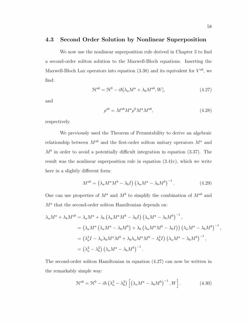
58

4.3 Second Order Solution by Nonlinear Superposition

We now use the nonlinear superposition rule derived in Chapter 3 to find

a second-order soliton solution to the Maxwell-Bloch equations. Inserting the

Maxwell-Bloch Lax operators into equation (3.38) and its equivalent for V ab, we

find:

Hab = H0 − i~[λaMa + λbM

ab,W ], (4.27)

and

ρab = MabMaρ0MaMab, (4.28)

respectively.

We previously used the Theorem of Permutability to derive an algebraic

relationship between Mab and the first-order soliton unitary operators Ma and

M b in order to avoid a potentially difficult integration in equation (3.37). The

result was the nonlinear superposition rule in equation (3.41c), which we write

here in a slightly different form:

Mab =(λaM

aM b − λbI) (λaM

a − λbM b)−1

. (4.29)

One can use properties of Ma and M b to simplify the combination of Mab and

Ma that the second-order soliton Hamiltonian depends on:

λaMa + λbM

ab = λaMa + λb

(λaM

aM b − λbI) (λaM

a − λbM b)−1

,

=(λaM

a(λaM

a − λbM b)

+ λb(λaM

aM b − λbI)) (

λaMa − λbM b

)−1,

=(λ2aI − λaλbMaM b + λbλaM

aM b − λ2bI) (λaM

a − λbM b)−1

,

=(λ2a − λ2

b

) (λaM

a − λbM b)−1

.

The second-order soliton Hamiltonian in equation (4.27) can now be written in

the remarkably simple way:

Hab = H0 − i~(λ2a − λ2

b

) [(λaM

a − λbM b)−1

,W]. (4.30)

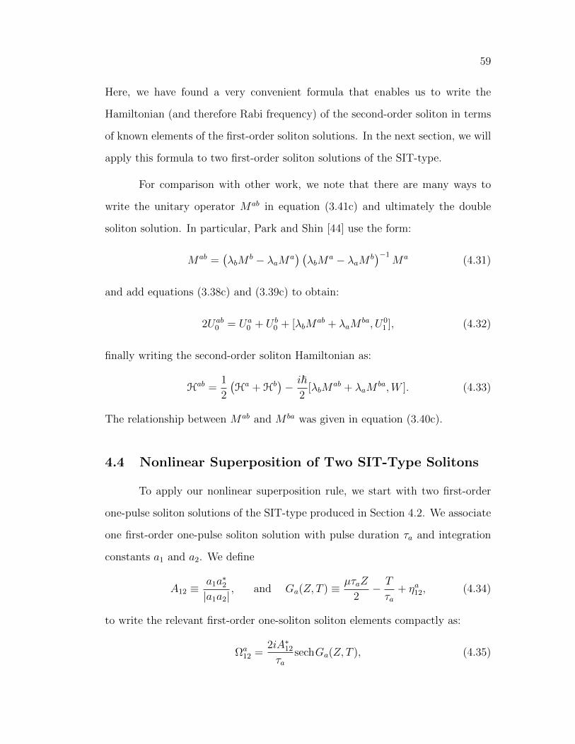
59

Here, we have found a very convenient formula that enables us to write the

Hamiltonian (and therefore Rabi frequency) of the second-order soliton in terms

of known elements of the first-order soliton solutions. In the next section, we will

apply this formula to two first-order soliton solutions of the SIT-type.

For comparison with other work, we note that there are many ways to

write the unitary operator Mab in equation (3.41c) and ultimately the double

soliton solution. In particular, Park and Shin [44] use the form:

Mab =(λbM

b − λaMa) (λbM

a − λaM b)−1

Ma (4.31)

and add equations (3.38c) and (3.39c) to obtain:

2Uab0 = Ua

0 + U b0 + [λbM

ab + λaMba, U0

1 ], (4.32)

finally writing the second-order soliton Hamiltonian as:

Hab =1

2

(Ha + Hb

)− i~

2[λbM

ab + λaMba,W ]. (4.33)

The relationship between Mab and M ba was given in equation (3.40c).

4.4 Nonlinear Superposition of Two SIT-Type Solitons

To apply our nonlinear superposition rule, we start with two first-order

one-pulse soliton solutions of the SIT-type produced in Section 4.2. We associate

one first-order one-pulse soliton solution with pulse duration τa and integration

constants a1 and a2. We define

A12 ≡a1a

∗2

|a1a2|, and Ga(Z, T ) ≡ µτaZ

2− T

τa+ ηa12, (4.34)

to write the relevant first-order one-soliton soliton elements compactly as:

Ωa12 =

2iA∗12

τasechGa(Z, T ), (4.35)

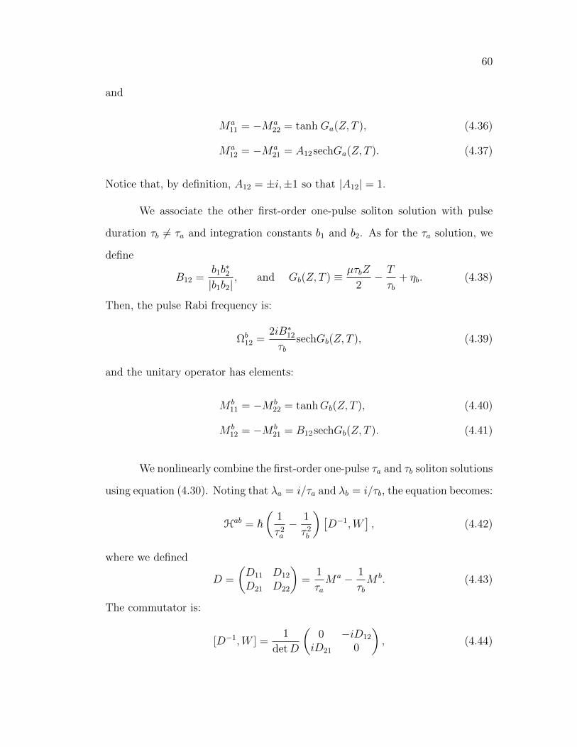
60

and

Ma11 = −Ma

22 = tanh Ga(Z, T ), (4.36)

Ma12 = −Ma

21 = A12 sechGa(Z, T ). (4.37)

Notice that, by definition, A12 = ±i,±1 so that |A12| = 1.

We associate the other first-order one-pulse soliton solution with pulse

duration τb 6= τa and integration constants b1 and b2. As for the τa solution, we

define

B12 =b1b∗2

|b1b2|, and Gb(Z, T ) ≡ µτbZ

2− T

τb+ ηb. (4.38)

Then, the pulse Rabi frequency is:

Ωb12 =

2iB∗12

τbsechGb(Z, T ), (4.39)

and the unitary operator has elements:

M b11 = −M b

22 = tanhGb(Z, T ), (4.40)

M b12 = −M b

21 = B12 sechGb(Z, T ). (4.41)

We nonlinearly combine the first-order one-pulse τa and τb soliton solutions

using equation (4.30). Noting that λa = i/τa and λb = i/τb, the equation becomes:

Hab = ~(

1

τ 2a

− 1

τ 2b

)[D−1,W

], (4.42)

where we defined

D =

(D11 D12

D21 D22

)=

1

τaMa − 1

τbM b. (4.43)

The commutator is:

[D−1,W ] =1

detD

(0 −iD12

iD21 0

), (4.44)

61

and so the second-order Hamiltonian can be written:

Hab =i~

detD

(1

τ 2a

− 1

τ 2b

)(0 −D12

D21 0

). (4.45)

The second-order two-pulse soliton pulse Rabi frequency is therefore:

Ωab12 = − 2i

detD

(1

τ 2a

− 1

τ 2b

)D21. (4.46)

After some simple rearranging, one finds that the determinant of the matrix is:

detD =1

τaτb(A12B

∗12 + A∗12B12) sechGa(Z, T ) sechGb(Z, T )

+2

τaτbtanhGa(Z, T ) tanhGb(Z, T )−

(1

τ 2a

+1

τ 2b

),

(4.47)

and the second-order two-pulse soliton Rabi frequency is finally:

Ωab12 =

(1τ2a− 1

τ2b

)

detD

(−2iA∗12

τasechGa(Z, T ) +

2iB∗12

τbsechGb(Z, T )

). (4.48)

We plot the Rabi frequency as a function of space and time in the laboratory

coordinates (x = Z, t = T + x/c) in Figure 4.2.

One can see that for large, negative t the Rabi frequency separates into

two hyperbolic secants, one moving faster than the other. Around x, t = 0 a

collision occurs as the faster hyperbolic secant catches up to the slower. After

the collision, the hyperbolic secants reemerge with the faster one now traveling

to the right of the slower. The asymptotic behavior of the Rabi frequency can be

calculated and one finds:

limT→±∞

Ωab12 = ε

(− 2iA∗12

τasech

(Ga(Z, T )∓ δab

)+

2iB∗12

τbsech

(Gb(Z, T )± δab

)),

(4.49)

where Gi(Z, T ) = T/τi − µτiZ/2 + ηi as before. We have defined

ε = sign(τa − τb), (4.50)

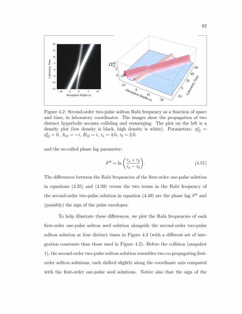
62

-10 -5 0 5 10-15

-10

-5

0

5

10

15

20

-4-2

02

4

-0.5

0.0

0.5

1.0

Absorption Depths kx

Single-Soliton Density Matrix

r22

ImHr12 L

r11

Labo

rato

ry T

ime

2

-4 -2 0 2 4-0.5

0.0

0.5

1.0taW12

ab

-4 -2 0 2 4

-0.5

0.0

0.5

1.0

Absorption Depths kx

Single-Soliton Density Matrix

r22

ImHr12 Lr11

Labo

rato

ry T

ime

0

–10

100

20

20

40

60

0

–20

Figure 4.2: Second-order two-pulse soliton Rabi frequency as a function of spaceand time, in laboratory coordinates. The images show the propagation of twodistinct hyperbolic secants colliding and reemerging. The plot on the left is adensity plot (low density is black, high density is white). Parameters: ηa12 =ηb12 = 0, A12 = −i, B12 = i, τa = 4.0, τb = 2.0.

and the so-called phase lag parameter:

δab = ln

(τa + τbτa − τb

). (4.51)

The differences between the Rabi frequencies of the first-order one-pulse solution

in equations (4.35) and (4.39) versus the two terms in the Rabi frequency of

the second-order two-pulse solution in equation (4.49) are the phase lag δab and

(possibly) the sign of the pulse envelopes.

To help illustrate these differences, we plot the Rabi frequencies of each

first-order one-pulse soliton seed solution alongside the second-order two-pulse

soliton solution at four distinct times in Figure 4.3 (with a different set of inte-

gration constants than those used in Figure 4.2). Before the collision (snapshot

1), the second-order two-pulse soliton solution resembles two co-propagating first-

order soliton solutions, each shifted slightly along the coordinate axis compared

with the first-order one-pulse seed solutions. Notice also that the sign of the

63

τa part of Ωab12 (right-most hyperbolic secant) has the opposite sign of its first-

order one-pulse soliton solution counterpart Ωa12. During the collision (snapshots

2 and 3) the second-order two-pulse soliton solution changes rapidly and cannot

be reduced to the simple sum of two hyperbolic secant pulses. After the collision

(snapshot 4), the second-order two-pulse soliton solution again simplifies into

two well-separated pulses differing from the first-order one-pulse soliton solutions

only in their relative phases and the sign of the τa part of Ωab12 (now the left-most

hyperbolic secant) with respect to Ωa12. Ultimately, the faster-moving τb pulse is

ahead (to the right) of the τa pulse.

We will not write the associated atomic density matrix elements explicitly,

but they can be calculated from equation (4.28). One finds that the atoms located

to the left of the collision undergo two full, separate population transfers as they

are excited by first the τa SIT-type pulse and later by the τb pulse. Near the

collision, the τa and τb components of the solution are overlapped and the reaction

of the atoms is significantly more complicated. After the collision, Ωab12 separates

back into two SIT-type pulses and the atoms again undergo two distinct cycles

of population transfer, first induced by the τb pulse and next by the pulse of

duration τa. The sign of the atomic coherence ρab12 is tied to the sign of the Rabi

frequency Ωab12 through Maxwell’s slowly-varying envelope equation. As a result,

if the sign of the Ωab12 envelope is different with respect to the seed solutions, then

there is associated change in the sign of the coherence term ρab12 with respect to

ρa12 and ρb12 before and after the collision.

64

-20 -10 0 10 20

-2

-1

0

1

2

3

4

-20 -10 0 10 20

-2

-1

0

1

2

3

4

-20 -10 0 10 20

-2

-1

0

1

2

3

4

-20 -10 0 10 20

-2

-1

0

1

2

3

4

-20 -10 0 10 20

-2

-1

0

1

2

3

4taW12

ab taW12a taW12

b

-20 -10 0 10 20

-2

-1

0

1

2

3

4taW12

ab taW12a taW12

b

-20 -10 0 10 20

-2

-1

0

1

2

3

4taW12

ab taW12a taW12

b

-20 -10 0 10 20

-2

-1

0

1

2

3

4taW12

ab taW12a taW12

b

-4 -2 0 2 4

-0.5

0.0

0.5

1.0

Absorption Depths kx

Single-Soliton Density Matrix

r22

ImHr12 Lr11

-4 -2 0 2 4

-0.5

0.0

0.5

1.0

Absorption Depths kx

Single-Soliton Density Matrix

r22

ImHr12 Lr11

-4 -2 0 2 4

-0.5

0.0

0.5

1.0

Absorption Depths kx

Single-Soliton Density Matrix

r22

ImHr12 Lr11

-4 -2 0 2 4

-0.5

0.0

0.5

1.0

Absorption Depths kx

Single-Soliton Density Matrix

r22

ImHr12 Lr11

-20 -10 0 10 20

-2

-1

0

1

2

3

4taW12

ab taW12a taW12

b

-20 -10 0 10 20

-2

-1

0

1

2

3

4taW12

ab taW12a taW12

b

Snapshot 1 Snapshot 2

Snapshot 3 Snapshot 4

Figure 4.3: Snapshots of the pulse Rabi frequencies of the second-order two-pulsesoliton and related first-order one-pulse soliton solutions at four distinct times.Parameters are different from those in Figure 4.2. Here, we chose τa = 4.0, τb =2.5 and integration constants a1 = 1, a2 = i, b1 = 1, b2 = −i so that A12 = −iand B12 = i and ηa12 = ηb12 = 0. Snapshots show the solutions before (snapshot1), during (snapshots 2 and 3), and after (snapshot 4) the collision at timesT/τa = −55,−6, 3, 55 (from 1 to 4, respectively) .

65

Chapter 5

Soliton Solutions for Optical Pulse Control

Multi-level media offer the opportunity for more complicated dynamics

and pulse-pulse interactions. In this chapter, we take a major step toward es-

tablishing a robust model for high-bandwidth optical pulse control by deriving

soliton solutions for storage and memory manipulation in Λ-type media. We take

up the issue of robustness of the solutions in the next chapter.

In Λ-type media, each soliton solution describes two different-frequency

fields and so a first-order soliton solution may have two pulses (one for each

field). This is in contrast with two-level media in which the first-order solitons

are always one-pulse (single frequency) solutions. Second-order soliton solutions

in Λ-media can therefore be two-, three-, or four-pulse solutions, depending on

how many pulses belong to each first-order seed solution being superimposed.

We start by deriving a special case of the first-order two-pulse soliton

solution derived by Clader and Eberly [45]. The solution shows one optical pulse

depleted but “stored” or “imprinted” in a process resulting in a redistribution

of the atomic ground state density matrix elements (populations ρ11, ρ22 and

off-diagonal coherence ρ12). Next, we derive a different (very simple) first-order

one-pulse soliton solution that models a “retrieval” pulse to be collided with the

stored pulse. We collide (superimpose) our two solutions to generate a novel

second-order three-pulse soliton solution. When the solitons collide, the retrieval

pulse pushes the imprint or memory of the stored pulse to a new (predictable)

66

location, redistributing the atomic ground state density matrix elements once

again.

5.1 Integrability of Λ-Type Media

In Chapter 2, we derived the nonlinear evolution equations governing co-

herent optical pulse propagation in Λ-media. We showed that for equal atom-field

coupling parameters the Maxwell-Bloch equations were:

i~∂ρ

∂T= [H, ρ], (2.62a)

and

∂H

∂Z= −~µ

2[W, ρ], (2.62b)

where

H =

0 0 −~d13 · ~E∗13

0 0 −~d23 · ~E∗23

−~d31 · ~E13 −~d32 · ~E23 ~∆

(2.62c)

and W = i |3〉 〈3|. These equations are identical in form to those governing pulse

propagation in two-level media (compare with equations (2.31)).

This symmetry can be attributed to the fact that both systems belong to

the SU(2)×U(1) group whenever µ1 = µ2, as we have assumed [44]. In previous

work, we showed that a four-level four-pulse system also belongs to this group and

derived an associated first-order soliton solution [49]. We will not explore these

connections further here except to note that because the equations have the same

form, we can easily prove integrability using the procedure already established

for two-level media.

The Lax operators have the same form for two and three-level media and

are:

U = − i~H − λW, (4.6b)

67

V =iµ

2λρ. (4.6b)

One can show that the Λ-media Maxwell-Bloch equations are equivalent to the

single Lax equation:

UZ − VT + [U, V ] = 0, (5.3)

by plugging in the Lax operators above and collecting like orders of the spectral

parameter λ. In Section 4.2, we derived a relationship between zero-order and

first-order soliton solutions for this Lax pair. We showed that:

ρa = Maρ0Ma, (4.15)

and

Ha = H0 +~τa

[Ma,W ]. (4.10)

In the above, ρ0 and H0 belong to a zero-order seed solution and we have identified

the inverse spectral parameter in terms of the soliton pulse duration, λa = i/τa,

as before.

The Hermitian unitary matrix operator that relates the zero- and first-

order soliton solutions is:

Ma = 2P a − I = 2|φa〉 〈φa|〈φa|φa〉 − I, (5.4)

where the wavefunction |φa〉 is a solution to the linear Lax equations evaluated

at λ = −λa = −i/τa:

∂ |φa〉∂T

=

(− i~H0 +

i

τaW

)|φa〉 , (5.5a)

∂ |φa〉∂Z

=(−µτa

2ρ0)|φa〉 . (5.5b)

68

5.2 First-Order Soliton Solution: Pulse Transfer and Stor-age

In previous work, Clader and Eberly derived first-order two-pulse soli-

ton solutions for Λ-media with two-photon resonance and modeled the effects

of significant inhomogeneous broadening [45, 50]. Their model applied to atoms

initially prepared in either mixed or pure states with conditions that they asso-

ciated with room temperature vapors. Here, we review a special case of one of

their first-order two-pulse soliton solutions for absorbing media under different

conditions: in the absence of Doppler broadening and with zero detuning. Such

conditions can be associated with a cloud of ultra-cold, near Bose-Einstein Con-

densate (BEC) temperature atoms and our solution has implications for optical

pulse storage and control in this regime.

To generate the first-order two-pulse soliton solution, we start with a sim-

ple seed in which both fields remain “off:”

Ω013(Z, T ) = 0, Ω0

23(Z, T ) = 0, (5.6a)

and the atoms remain in the ground state:

ρ0(Z, T ) =

1 0 00 0 00 0 0

. (5.6b)

The linear Lax equations are easy to solve for this simple seed solution. The

wavefunction solution to equations (5.5) is:

|φa〉 =

a1e−µτaZ/2

a2

a3e−T/τa

, (5.7)

with constants of integration a1, a2, a3.

The first-order two-pulse soliton density matrix and Hamiltonian are:

ρa = Maρ0Ma =

|Ma

11|2 Ma11M

a12 Ma

11Ma13

Ma11M

a∗12 |Ma

12|2 Ma13M

a∗12

Ma11M

a∗13 Ma∗

13Ma12 |Ma

13|2

, (5.8)

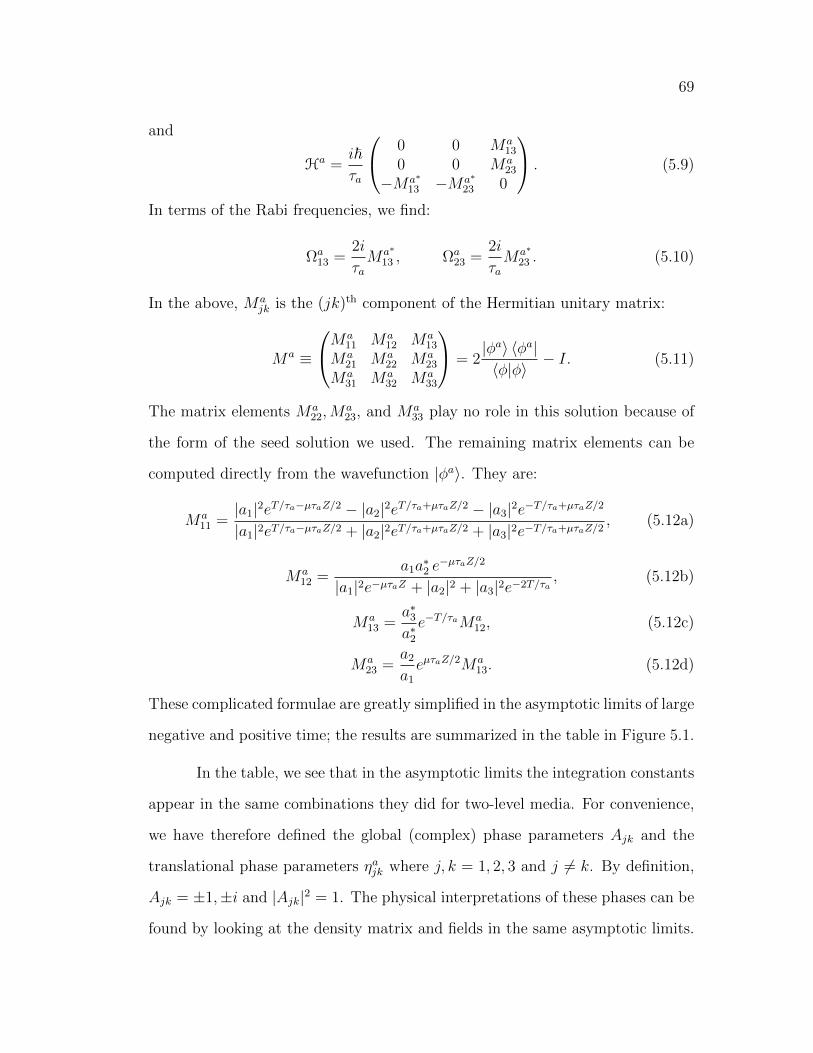
69

and

Ha =i~τa

0 0 Ma13

0 0 Ma23

−Ma∗13 −Ma∗

23 0

. (5.9)

In terms of the Rabi frequencies, we find:

Ωa13 =

2i

τaMa∗

13 , Ωa23 =

2i

τaMa∗

23 . (5.10)

In the above, Majk is the (jk)th component of the Hermitian unitary matrix:

Ma ≡

Ma

11 Ma12 Ma

13

Ma21 Ma

22 Ma23

Ma31 Ma

32 Ma33

= 2

|φa〉 〈φa|〈φ|φ〉 − I. (5.11)

The matrix elements Ma22,M

a23, and Ma

33 play no role in this solution because of

the form of the seed solution we used. The remaining matrix elements can be

computed directly from the wavefunction |φa〉. They are:

Ma11 =

|a1|2eT/τa−µτaZ/2 − |a2|2eT/τa+µτaZ/2 − |a3|2e−T/τa+µτaZ/2

|a1|2eT/τa−µτaZ/2 + |a2|2eT/τa+µτaZ/2 + |a3|2e−T/τa+µτaZ/2, (5.12a)

Ma12 =

a1a∗2 e−µτaZ/2

|a1|2e−µτaZ + |a2|2 + |a3|2e−2T/τa, (5.12b)

Ma13 =

a∗3a∗2e−T/τaMa

12, (5.12c)

Ma23 =

a2

a1

eµτaZ/2Ma13. (5.12d)

These complicated formulae are greatly simplified in the asymptotic limits of large

negative and positive time; the results are summarized in the table in Figure 5.1.

In the table, we see that in the asymptotic limits the integration constants

appear in the same combinations they did for two-level media. For convenience,

we have therefore defined the global (complex) phase parameters Ajk and the

translational phase parameters ηajk where j, k = 1, 2, 3 and j 6= k. By definition,

Ajk = ±1,±i and |Ajk|2 = 1. The physical interpretations of these phases can be

found by looking at the density matrix and fields in the same asymptotic limits.

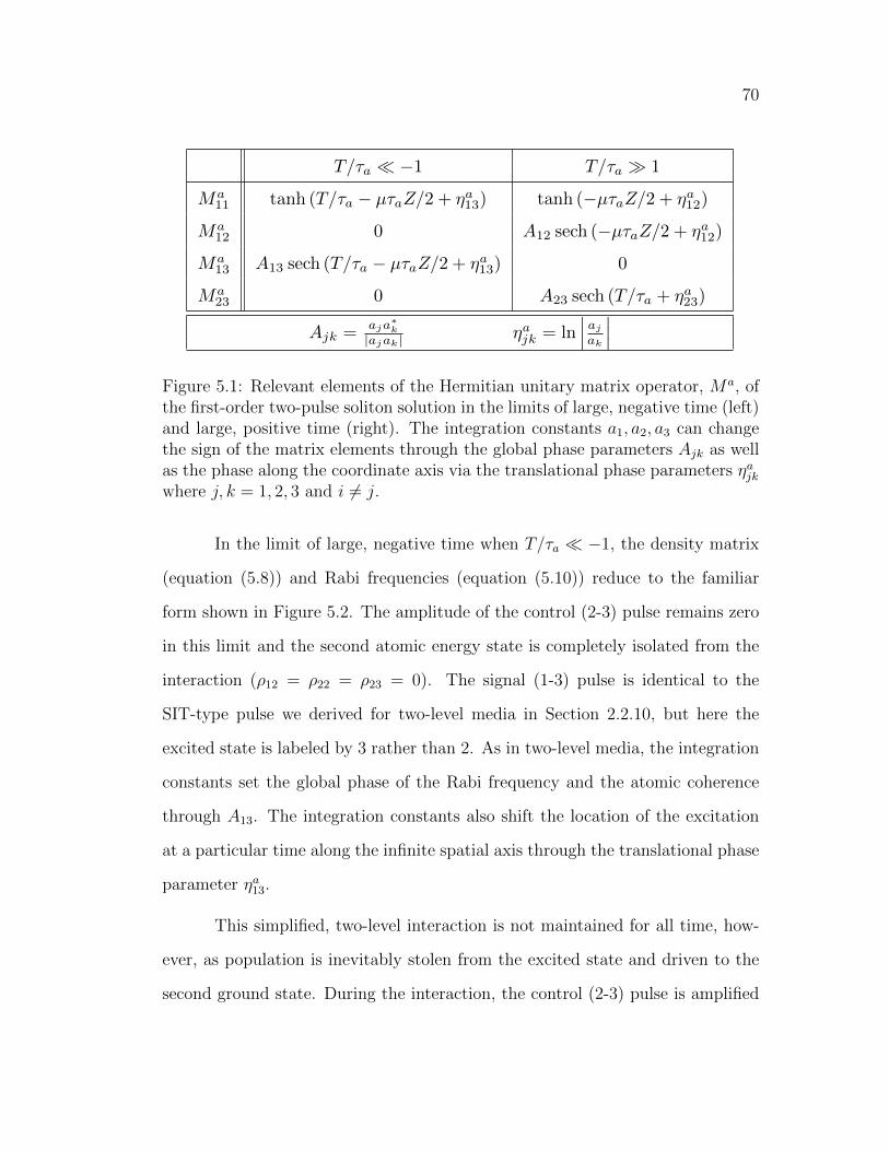
70

T/a 1 T/a 1

Ma11 tanh (T/a µaZ/2 + a

13) tanh (µaZ/2 + a12)

Ma12 0 A12 sech (µaZ/2 + a

12)

Ma13 A13 sech (T/a µaZ/2 + a

13) 0

Ma23 0 A23 sech (T/a + a

23)

Ajk =aja

k

|ajak| ajk = ln

aj

ak

T/a 1

a11 tanh2 (µaZ/2 + a

12)

a12 A12 sech (µaZ/2 + a

12) tanh (µaZ/2 + a12)

a22 sech2 (µaZ/2 + a

12)

a23 (2iA

23/a) sech (T/a + a23)

A12 = 1 a12 = 0 B12 = 0 b

12 = 0

A13 = i a12 = 0 B13 = 0 b

12 = 0

A12 = i a12 = 0 B23 = i b

12 = 18.42

(1)

A12 = 1, a12 = 1 (2)

(3)

T/a 1

a11 tanh2 (µaZ/2 a

12)

a12 A12 sech (µaZ/2 a

12) tanh (µaZ/2 a12)

a22 sech2 (µaZ/2 a

12)

a23 (2iA

23/a) sech (T/a + a23)

1

Figure 5.1: Relevant elements of the Hermitian unitary matrix operator, Ma, ofthe first-order two-pulse soliton solution in the limits of large, negative time (left)and large, positive time (right). The integration constants a1, a2, a3 can changethe sign of the matrix elements through the global phase parameters Ajk as wellas the phase along the coordinate axis via the translational phase parameters ηajkwhere j, k = 1, 2, 3 and i 6= j.

In the limit of large, negative time when T/τa −1, the density matrix

(equation (5.8)) and Rabi frequencies (equation (5.10)) reduce to the familiar

form shown in Figure 5.2. The amplitude of the control (2-3) pulse remains zero

in this limit and the second atomic energy state is completely isolated from the

interaction (ρ12 = ρ22 = ρ23 = 0). The signal (1-3) pulse is identical to the

SIT-type pulse we derived for two-level media in Section 2.2.10, but here the

excited state is labeled by 3 rather than 2. As in two-level media, the integration

constants set the global phase of the Rabi frequency and the atomic coherence

through A13. The integration constants also shift the location of the excitation

at a particular time along the infinite spatial axis through the translational phase

parameter ηa13.

This simplified, two-level interaction is not maintained for all time, how-

ever, as population is inevitably stolen from the excited state and driven to the

second ground state. During the interaction, the control (2-3) pulse is amplified

71

as it cycles more and more atomic population between levels 2 and 3. The Rabi

frequencies and populations of levels 2 and 3 at three distinct times during the

amplification process are shown graphically in Figure 5.3. For later comparison

with our numerical solutions, the solution is shown graphically in the laboratory

coordinates t and x where T = t− x/c and Z = x.

1

3

2

T/a 1 T/a 1

Ma11 tanh (T/a µaZ/2 + a

13) tanh (µaZ/2 + a12)

Ma12 0 A12 sech (µaZ/2 + a

12)

Ma13 A13 sech (T/a µaZ/2 + a

13) 0

Ma23 0 A23 sech (T/a + a

23)

Ajk =aja

k

|ajak| ajk = ln

aj

ak

T/a 1

a11 tanh2 (Ga(Z, T ))

a13 A13 sech (Ga(Z, T )) tanh (Ga(Z, T ))

a33 sech2 (Ga(Z, T ))

a13 (2iA

13/a) sech (Ga(Z, T ))

Ga(Z, T ) = T/a µaZ/2 + a13

T/a 1

a11 tanh2 (µaZ/2 + a

12)

a12 A12 sech (µaZ/2 + a

12) tanh (µaZ/2 + a12)

a22 sech2 (µaZ/2 + a

12)

a23 (2iA

23/a) sech (T/a + a23)

A12 = 1 a12 = 0 B12 = 0 b

12 = 0

A13 = i a12 = 0 B13 = 0 b

12 = 0

A12 = i a12 = 0 B23 = i b

12 = 18.42

(1)

A12 = 1, a12 = 1 (2)

(3)

1

Figure 5.2: First-order two-pulse soliton solution in the limit of large, negativetime. Only the signal (1-3) pulse is present and the interaction is identical to thetwo-level SIT solution. The remaining elements (Ω23, ρ12, ρ22, ρ23, not shown) goto zero in this limit.

The transfer of pulse excitation is total; the initially 2π-area SIT-type

signal (1-3) pulse is ultimately totally depleted and the control (2-3) pulse is

amplified until its area grows to 2π. The pulse Rabi frequencies and atomic

density matrix elements of the second-order two-pulse solution in the long-time

limit, T/τa 1, are summarized in the table in Figure 5.4 and shown graphically

in Figure 5.5. The control (2-3) pulse travels at the speed of light in vacuum

because it is completely decoupled from the medium in the long-time limit. Its

position along the coordinate axis can be shifted by the integration constants

through the translational phase parameter ηa23.

An important intermediate result has been achieved here. The transfer of

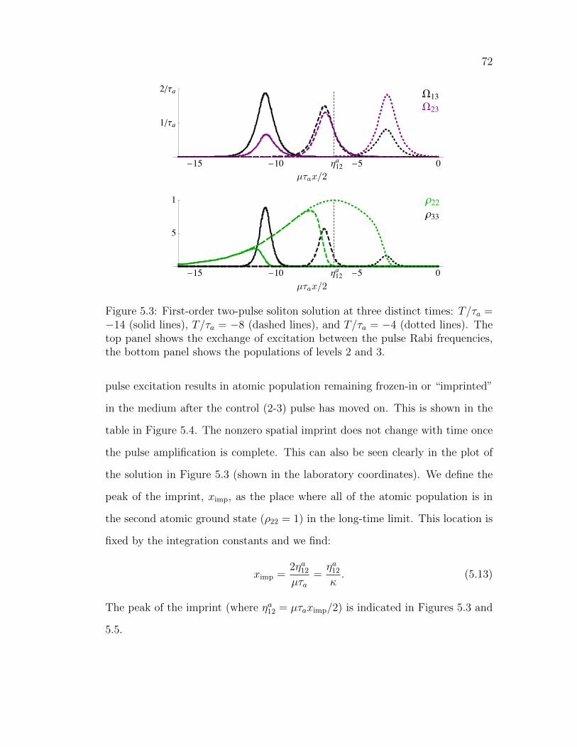
72

-15 -10 -5-h12a 0

0.5

1

-15 -10 -5-h12a 0

1êta

2êta

µax/2 (1)

T/a 1

a11 tanh2 (Ga(Z, T ) + a

13)

a13 A13 sech (Ga(Z, T ) + a

13) tanh (Ga(Z, T ) + a13)

a33 sech2 (Ga(Z, T ) + a

13)

a13 (2iA13/a) sech (Ga(Z, T ) + a

13)

Ga(Z, T ) = T/a µaZ/2

a11 tanh2 (µaZ/2 a

12)

a12 A12 sech (µaZ/2 a

12) tanh (µaZ/2 a12)

a13 A13 sech2 (T/a µaZ/2 + a

12)

T/a 1

a11 tanh2 (T/a µaZ/2 + a

12)

a13 A13 sech (T/a µaZ/2 + a

13) tanh (T/a µaZ/2 + a12)

a13 A13 sech2 (T/a µaZ/2 + a

12)

a13 = 0 (2)

a12 = 0

a22 = 0

a23 = 0

a23 = 0

(x) (3)

↵x/2 (4)

! (5)

(6)

1

µax/2 (1)

T/a 1

a11 tanh2 (Ga(Z, T ) + a

13)

a13 A13 sech (Ga(Z, T ) + a

13) tanh (Ga(Z, T ) + a13)

a33 sech2 (Ga(Z, T ) + a

13)

a13 (2iA13/a) sech (Ga(Z, T ) + a

13)

Ga(Z, T ) = T/a µaZ/2

a11 tanh2 (µaZ/2 a

12)

a12 A12 sech (µaZ/2 a

12) tanh (µaZ/2 a12)

a13 A13 sech2 (T/a µaZ/2 + a

12)

T/a 1

a11 tanh2 (T/a µaZ/2 + a

12)

a13 A13 sech (T/a µaZ/2 + a

13) tanh (T/a µaZ/2 + a12)

a13 A13 sech2 (T/a µaZ/2 + a

12)

a13 = 0 (2)

a12 = 0

a22 = 0

a23 = 0

a23 = 0

(x) (3)

↵x/2 (4)

! (5)

(6)

1

-15 -10 -5-d12a 0

ta

2taW13

-15 -10 -5-d12a 0

0

0.5

1r22

-15 -10 -5-d12a 0

ta

2taW23

-15 -10 -5-d12a 0

0.5

1r33

Figure 5.3: First-order two-pulse soliton solution at three distinct times: T/τa =−14 (solid lines), T/τa = −8 (dashed lines), and T/τa = −4 (dotted lines). Thetop panel shows the exchange of excitation between the pulse Rabi frequencies,the bottom panel shows the populations of levels 2 and 3.

pulse excitation results in atomic population remaining frozen-in or “imprinted”

in the medium after the control (2-3) pulse has moved on. This is shown in the

table in Figure 5.4. The nonzero spatial imprint does not change with time once

the pulse amplification is complete. This can also be seen clearly in the plot of

the solution in Figure 5.3 (shown in the laboratory coordinates). We define the

peak of the imprint, ximp, as the place where all of the atomic population is in

the second atomic ground state (ρ22 = 1) in the long-time limit. This location is

fixed by the integration constants and we find:

ximp =2ηa12

µτa=ηa12

κ. (5.13)

The peak of the imprint (where ηa12 = µτaximp/2) is indicated in Figures 5.3 and

5.5.

73

a12 = 0 b

23 = 4.16

a1 = 1 a2 = 5 a3 = i/5

b1 = 0 b2 = 1 b3 = 1

a = 2 b = 1 T/a = 25

a1 = 1 a2 = 5 a3 = i/5

b1 = 0 b2 = 1 b3 = 1

a = 2 b = 1 T/a = 25

T/a 1 T/a 1

Ma11 tanh (T/a µaZ/2 + a

13) tanh (µaZ/2 + a12)

Ma12 0 A12 sech (µaZ/2 + a

12)

Ma13 A13 sech (T/a µaZ/2 + a

13) 0

Ma23 0 A23 sech (T/a + a

23)

Ajk =aja

k

|ajak| ajk = ln

aj

ak

T/a 1

a11 tanh2 (Ga(Z, T ))

a13 A13 sech (Ga(Z, T )) tanh (Ga(Z, T ))

a33 sech2 (Ga(Z, T ))

a13 (2iA

13/a) sech (Ga(Z, T ))

Ga(Z, T ) = T/a µaZ/2 + a13

T/a 1

a11 tanh2 (µaZ/2 + a

12)

a12 A12 sech (µaZ/2 + a

12) tanh (µaZ/2 + a12)

a22 sech2 (µaZ/2 + a

12)

a23 (2iA

23/a) sech (T/a + a23)

2

1

3

2

Figure 5.4: First-order soliton solution in the long-time limit. The ground-statedensity matrix elements (shown) have a nontrivial spatial dependence and theremaining density matrix elements (ρ13 = ρ23 = ρ33 = 0, not shown) are identi-cally zero. The signal (1-3) pulse (not shown) has been depleted and the control(2-3) pulse is decoupled with area 2π.

5.3 Pulse Area and Time-Matched Pulses

We have already noted that the Rabi frequencies in the asymptotic limits

and reduce to 2π-area pulses (see Figures 5.1 and 5.4). The pulse area plays

an important role even outside of those special limits. In particular, Clader and

Eberly defined the “total” pulse area:

θ(Z) =√|θa13(Z)|2 + |θa23(Z)|2 (5.14)

where θa13 and θa23 are the individual pulse areas of each Rabi frequency. They

showed that although the individual pulse areas change throughout the pulse-

transfer process, the total pulse area is constant throughout the medium and

always equal to exactly 2π.

In addition, they showed that the pulse Rabi frequencies depend on time

in exactly the same way and travel together even during the complicated pulse

transfer process. Such pulses are said to be time-matched and their ratio has

only a spatial dependence. For the first-order soliton solution, one finds that the

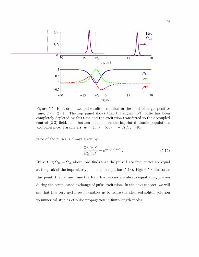
74

-15 -h12a 0 15 30

1êta2êta

-30 -15 -h12a 0 15 30

-0.5

0

0.5

1

-30 -15 -d12a 0 15 30

-0.5

0

0.5

1

µax/2 (1)

T/a 1

a11 tanh2 (Ga(Z, T ) + a

13)

a13 A13 sech (Ga(Z, T ) + a

13) tanh (Ga(Z, T ) + a13)

a33 sech2 (Ga(Z, T ) + a

13)

a13 (2iA13/a) sech (Ga(Z, T ) + a

13)

Ga(Z, T ) = T/a µaZ/2

a11 tanh2 (µaZ/2 a

12)

a12 A12 sech (µaZ/2 a

12) tanh (µaZ/2 a12)

a13 A13 sech2 (T/a µaZ/2 + a

12)

T/a 1

a11 tanh2 (T/a µaZ/2 + a

12)

a13 A13 sech (T/a µaZ/2 + a

13) tanh (T/a µaZ/2 + a12)

a13 A13 sech2 (T/a µaZ/2 + a

12)

a13 = 0 (2)

a12 = 0

a22 = 0

a23 = 0

a23 = 0

(x) (3)

↵x/2 (4)

! (5)

(6)

1

µax/2 (1)

T/a 1

a11 tanh2 (Ga(Z, T ) + a

13)

a13 A13 sech (Ga(Z, T ) + a

13) tanh (Ga(Z, T ) + a13)

a33 sech2 (Ga(Z, T ) + a

13)

a13 (2iA13/a) sech (Ga(Z, T ) + a

13)

Ga(Z, T ) = T/a µaZ/2

a11 tanh2 (µaZ/2 a

12)

a12 A12 sech (µaZ/2 a

12) tanh (µaZ/2 a12)

a13 A13 sech2 (T/a µaZ/2 + a

12)

T/a 1

a11 tanh2 (T/a µaZ/2 + a

12)

a13 A13 sech (T/a µaZ/2 + a

13) tanh (T/a µaZ/2 + a12)

a13 A13 sech2 (T/a µaZ/2 + a

12)

a13 = 0 (2)

a12 = 0

a22 = 0

a23 = 0

a23 = 0

(x) (3)

↵x/2 (4)

! (5)

(6)

1

-15 -10 -5-d12a 0

ta

2taW13

-15 -10 -5-d12a 0

ta

2taW23

-15 -10 -5-d12a 0

0

0.5

1r22

-15 -d12a 0 15 30

1êta2êta

-15 -10 -5-d12a 0

0.5

1r11

-15 -10 -5-d12a 0

0.5

1r12

Figure 5.5: First-order two-pulse soliton solution in the limit of large, positivetime, T/τa 1. The top panel shows that the signal (1-3) pulse has beencompletely depleted by this time and the excitation transferred to the decoupledcontrol (2-3) field. The bottom panel shows the imprinted atomic populationsand coherence. Parameters: a1 = 1, a2 = 5, a3 = −i, T/τa = 40.

ratio of the pulses is always given by:

Ωa13(x, t)

Ωa23(x, t)

= e−µτax/2+ηa12 . (5.15)

By setting Ω13 = Ω23 above, one finds that the pulse Rabi frequencies are equal

at the peak of the imprint, ximp, defined in equation (5.13). Figure 5.3 illustrates

this point, that at any time the Rabi frequencies are always equal at ximp, even

during the complicated exchange of pulse excitation. In the next chapter, we will

see that this very useful result enables us to relate the idealized soliton solution

to numerical studies of pulse propagation in finite-length media.

75

5.4 First-Order Soliton Solution: Retrieval Pulse

In the previous section, we studied a particular first-order two-pulse soliton

solution with three independent integration constants. Now we obtain a simple,

but new first-order one-pulse soliton solution by setting one of the integration

constants equal to zero. This solution will serve as a “retrieval” solution and its

usefulness will be clear in the next section when we collide it with the first-order

two-pulse storage solution.

We start by setting the first integration constant, a1, in equation (5.7)

to zero. We will use the labeling a2 → b2, a3 → b3, and τa → τb to distin-

guish this solution from the previous one. Then, the first-order one-pulse soliton

wavefunction is:

|φb〉 =

0b2

b3e−T/τb

. (5.16)

and the associated Hermitian unitary matrix operator is M b = 2 |φb〉〈φb|〈φb|φb − I. As

before, we define a translational phase parameter ηb23 = ln∣∣∣ b2b3∣∣∣ and a global phase

parameter B23 =b2b∗3|b2b3| . The pulse Rabi frequencies and atomic density matrix

elements are calculated from the Hermitian unitary operator:

Ωb13 =

2i

τbM b∗

13 , Ωb23 =

2i

τbM b∗

23 , (5.17)

and

ρb = ρ0M bρ0. (5.18)

as before.

In this simple solution, the atomic population remains in the ground state,

the signal pulse stays “off,” and the uncoupled control field is a 2π-area hyperbolic

secant pulse for all time:

ρ(Z, T ) = |1〉 〈1| , Ω13(Z, T ) = 0, (5.19a)

76

Ω23(Z, T ) =2i

τbB∗23 sech

(T/τb + ηb23

). (5.19b)

The translational phase shift parameter ηb23 shifts the initial location of the control

(2-3) pulse along the infinite spatial axis while B23 = ±1,±i fixes its overall

(global) phase.

5.5 Second-Order Soliton Solution

We now superimpose the first-order two-pulse soliton solution (τa) with

the first-order one-pulse soliton solution (τb) to generate a new, exact, second-

order three-pulse soliton solution. The procedure we follow is the same as it was

for the two-level atom. The Hamiltonian of the second-order soliton solution is:

Hab = ~(

1

τ 2a

− 1

τ 2b

)[(1

τaMa − 1

τbM b

)−1

,W

], (5.20)

where Ma and M b are the first-order soliton Hermitian unitary matrices already

derived. To calculate the density matrix of the second-order soliton solution, we

use:

ρab = MabMaρ0MaMab, (5.21)

where ρ0 is the zero-order soliton solution that was used to produce the first-order

τa and τb soliton solutions: ρ0 = |1〉 〈1|. The Hermitian unitary matrix associated

with the second-order soliton solution is:

Mab =

(1

τaMaM b − 1

τbI

)(1

τaMa − 1

τbM b

)−1

. (5.22)

The density matrix elements and Hamiltonian can be calculated in a straightfor-

ward, albeit tedious way using the equations above. To simplify the discussion,

we will require τa > τb hereafter, as appropriate to the most interesting scenario,

in which the slower τa pulse is overtaken and modified by the τb pulse.

77

5.6 How to Choose the Integration Constants

We can anticipate that the solution will simplify in the limits of large neg-

ative and positive time (before and after the first-order soliton solutions collide),

as we saw with the two-level atom. There are, however, several complications in

three-level media that were not present in the two-level case. In two-level me-

dia, the τa and τb soliton solutions being superimposed were SIT-type solutions

with the same behavior, but different group velocities and phase shifts along the

infinite coordinate axis. The definition of “collision” was fairly straightforward

and simply identified the time (and place) at which the faster-moving hyperbolic

secant solution overtook the slower-moving one. For the three-level system, on

the other hand, the first-order soliton solutions have radically different behavior

from one another. The first-order one-pulse τb solution is a simple hyperbolic

secant pulse decoupled from the medium traveling at the speed of light in vac-

uum. In contrast, the τa two-pulse soliton solution changes dramatically as the

pulse excitation is transferred from the signal (1-3) field to the control (2-3) field.

An important point to consider, then, is what “collision” means for three-level

media.

Our central goal is to use soliton solutions for optical pulse control, and

we want to retain the imprinting process of the τa first-order two-pulse soliton

solution. That is, we want the storage/transfer process of the τa soliton solution

to be nearly complete before the τb soliton solution “catches up to” (or collides

with) it. The location of the imprint is controlled by ηa12, while the initial position

of the retrieval pulse solution is also fixed by the integration constants through

the translational phase parameter ηb23. To ensure that the imprint is initially far

ahead of the oncoming τb control (2-3) pulse, we require that:

ηa12 ηb23. (5.23)

78

Soliton solutions not meeting the restriction above are available, but do not model

the types of behavior we are concerned with here.

In the figures that follow, we choose integration constants:

a1 = 1, a2 = 1, a3 = i, (5.24a)

b1 = 0, b2 = 1× 10−4, b3 = i× 10−4, (5.24b)

so that the relevant parameters are:

A12 = 1, A13 = −i, A23 = −i, (5.25a)

ηa12 = 0, ηa13 = 0, ηa23 = 0, (5.25b)

B23 = i, ηb23 = −18.41. (5.25c)

For the interested reader, a few solutions not meeting the requirement in equation

(5.25) are described in Section 5.9 at the end of this chapter.

5.7 Before Collision: Signal Pulse Storage

If we choose the integration constants appropriately, then initially the

faster-moving τb component will be far behind (to the left of) the τa component

of the second-order soliton solution. In particular, if we satisfy conditions (5.25),

then the τa solution will have time to exhibit the full storage/transfer process

before the τb control (2-3) pulse collides with it. In Figure 5.6, we show the Rabi

frequencies of the second-order soliton solution under such conditions.

In the first frame shown (before the pulse storage process takes over), the

pulse Rabi frequencies are simply:

Ωab13 =

2i

τaA∗13sech

(T/τa − µτaZ/2 + ηa13 − δab

), (5.26a)

79

Signal

-4 -2 2 4

1

2

3

4

5

6ta W13

ab

Control

-4 -2 2 4

1

2

3

4

5

6ta W23

ab

ln |R1| (1)

x1 = ln R + ab = (2)

13/23 = |R1| (3)

1/b (4)

a12 (5)

a1 = 1, a2 = 5, a3 = i/5, (6)

a1 = 1, a2 = 5, a3 =1

5i, (7)

b1 = 0, b2 = 1, b3 = i, (8)

a = 2 b = 1, T = 25a, (9)

a1 = 1, a2 = 5, a3 =1

5i, (10)

b1 = 0, b2 = 1, b3 = i, (11)

a1 = 1 (12)

a2 = 2 (13)

aab13 (14)

↵x/2 (15)

! (16)

(17)

!3 (18)

!12 (19)

!23 (20)

(21)

23 (22)

1 (23)

loc1 (24)

1

-4 -2 2 4

1

2

3

4

5

6r22 ab

-4 -2 2 4

1

2

3

4

5

6r12

ab

-4 -2 2 4

1

2

3

4

5

6r12 ab

-4 -2 2 4

1

2

3

4

5

6r11 ab

-4 -2 2 4

1

2

3

4

5

6r11 ab

-4 -2 2 4

1

2

3

4

5

6r11 ab

Stored Signal Pulse Imprint

20

In this document, I print the equation first in black and then in white (whichof course we can’t see on the white background)

Im(13) (1)

Im(23) (2)

x (3)

23 (4)

33 (5)

(6)

@

@x+

1

c

@

@t

= iµ12 (7)

@

@x+

1

c

@

@t

= iµ12 (8)

=

Z(x, t)dt (9)

=

Z(x, t)dt (10)

vg =c

1 + (11)

vg =c

1 + (12)

xpeak = ln

inj

13

inj23

(13)

xpeak = ln

inj

13

inj23

(14)

= µ/2 (15)

1

100-10-20-30-40-50-60-70

Laboratory Tim

e t

0.0

2.0

1.0

In this document, I print the equation first in black and then in white (whichof course we can’t see on the white background)

Im(13) (1)

Im(23) (2)

x (3)

23 (4)

33 (5)

(6)

@

@x+

1

c

@

@t

= iµ12 (7)

@

@x+

1

c

@

@t

= iµ12 (8)

=

Z(x, t)dt (9)

=

Z(x, t)dt (10)

vg =c

1 + (11)

vg =c

1 + (12)

xpeak = ln

inj

13

inj23

(13)

xpeak = ln

inj

13

inj23

(14)

= µ/2 (15)

1

-5 0 5-0.5

0.0

0.5

1.0

-4 -2 2 4

1

2

3

4

5

6taW13

ab

-4 -2 2 4

1

2

3

4

5

6taW13

ab

Before Collision: Signal Pulse Storage

Figure 5.6: Pre-collision behavior of the second-order three-pulse soliton solution.The τb control (2-3) pulse remains at the far left of the τa signal (1-3) and control(2-3) pulses during the pulse storage process. The stored-pulse information isencoded on the atomic ground-state density matrix elements as shown (rightinset, T/τa = 1.5). Solutions are plotted in the laboratory coordinates with theparameters indicated in equation (5.25) with τa = 2, τb = 1.8 and snapshots takenwhen T/τa= -10.5, -9, -7.5, -6, -1.5, 0, 1.5 (front to back).

Ωab23 = −2i

τbB∗23sech

(T/τb + ηb23

). (5.26b)

The coupled signal (1-3) pulse drives population between atomic states 1 and 3

and differs merely by the phase lag δab from the T/τa −1 limit of the first-order

τa solution (see Figure 5.2), where:

δab = ln

(τa + τbτa − τb

). (5.27)

The decoupled control pulse does not have a phase lag associated with it, and

this asymmetry can be attributed to the asymmetry of the first-order soliton

solutions. The role of the phase lag in three-level media will be discussed further

in the next section. Notice that the sign of the τb control pulse is flipped relative

to its first-order soliton solution counterpart (see equation (5.19b)), just as it was

for two-level media.

As expected, the signal (1-3) pulse is depleted and its information encoded

on the atomic ground-state density matrix elements, as shown in the inset in

80

Figure 5.6. The distribution of the atomic states are shown after the τa signal

pulse has been stored, but before the τb control pulse reaches its imprint. At that

time, the ground-state populations and coherence are identical to the long-time

limit of their associated first-order soliton solution (refer to the table in Figure

5.4):

ρab11 = tanh2(−µτaZ/2 + ηa12), (5.28a)

ρab12 = A12sech(−µτaZ/2 + ηa12) tanh(−µτaZ/2 + ηa12), (5.28b)

ρab22 = tanh(−µτaZ/2 + ηa12). (5.28c)

As before, we define the location of the imprint (or pulse storage location) by

where ρab22 = 1 and find:

ximp =2

µτaηa12 = −1

κηa12. (5.29)

5.8 During and After Collision: Memory Manipulation

Eventually, the τb control (2-3) pulse catches up with the τa soliton solution

and collides with the imprint encoded on the atomic ground-state density matrix

elements. When the collision occurs, the τb control pulse begins to be depleted

as it reads and partially recovers the τa signal (1-3) pulse. The excitation is

soon transferred once again, as the τa signal pulse is redeposited (re-stored) in

the medium. The signal (1-3) pulse Rabi frequency, Ωab13, and the population

of the second ground state, ρab22, of the second-order soliton solution during this

process are shown in Figure 5.7. The figure shows that as the control pulse reads

the imprint, the signal pulse is recovered and quickly redeposited. The level 2

population has the same form in the initial (T/τa = 12.5) and final (T/τa = 24.5)

snapshots, merely shifted along the coordinate axis.

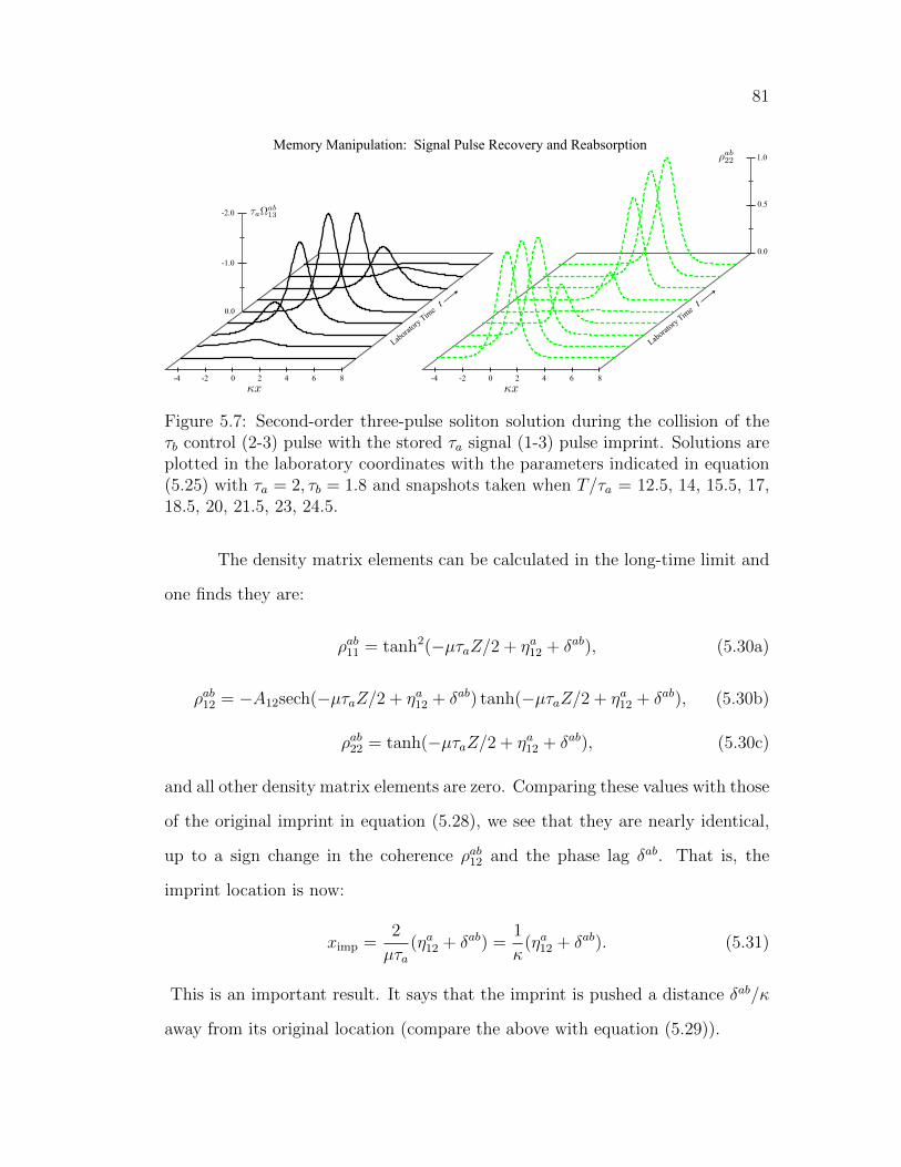
81

2 4 6 8

In this document, I print the equation first in black and then in white (whichof course we can’t see on the white background)

Im(13) (1)

Im(23) (2)

x (3)

23 (4)

33 (5)

(6)

@

@x+

1

c

@

@t

= iµ12 (7)

@

@x+

1

c

@

@t

= iµ12 (8)

=

Z(x, t)dt (9)

=

Z(x, t)dt (10)

vg =c

1 + (11)

vg =c

1 + (12)

xpeak = ln

inj

13

inj23

(13)

xpeak = ln

inj

13

inj23

(14)

= µ/2 (15)

1

0-2-4

1.0

0.5

0.0

In this document, I print the equation first in black and then in white (whichof course we can’t see on the white background)

ab22 (1)

↵x/2 (2)

! (3)

(4)

!3 (5)

!12 (6)

!23 (7)

(8)

23 (9)

1 (10)

loc1 (11)

0.5 (12)

|131|2 (13)

Im(13) (14)

Im(23) (15)

x (16)

t

1(17)

t/1 (18)

23 (19)

33 (20)

(21)

@

@x+

1

c

@

@t

= iµ12 (22)

@

@x+

1

c

@

@t

= iµ12 (23)

1

Laboratory Tim

e t

0.0

2 4 6 80-2-4

Laboratory Tim

e t

-2.0

-1.0

In this document, I print the equation first in black and then in white (whichof course we can’t see on the white background)

aab13 (1)

↵x/2 (2)

! (3)

(4)

!3 (5)

!12 (6)

!23 (7)

(8)

23 (9)

1 (10)

loc1 (11)

0.5 (12)

|131|2 (13)

Im(13) (14)

Im(23) (15)

x (16)

t

1(17)

t/1 (18)

23 (19)

33 (20)

(21)

@

@x+

1

c

@

@t

= iµ12 (22)

@

@x+

1

c

@

@t

= iµ12 (23)

1

In this document, I print the equation first in black and then in white (whichof course we can’t see on the white background)

Im(13) (1)

Im(23) (2)

x (3)

23 (4)

33 (5)

(6)

@

@x+

1

c

@

@t

= iµ12 (7)

@

@x+

1

c

@

@t

= iµ12 (8)

=

Z(x, t)dt (9)

=

Z(x, t)dt (10)

vg =c

1 + (11)

vg =c

1 + (12)

xpeak = ln

inj

13

inj23

(13)

xpeak = ln

inj

13

inj23

(14)

= µ/2 (15)

1

Memory Manipulation: Signal Pulse Recovery and Reabsorption

Figure 5.7: Second-order three-pulse soliton solution during the collision of theτb control (2-3) pulse with the stored τa signal (1-3) pulse imprint. Solutions areplotted in the laboratory coordinates with the parameters indicated in equation(5.25) with τa = 2, τb = 1.8 and snapshots taken when T/τa = 12.5, 14, 15.5, 17,18.5, 20, 21.5, 23, 24.5.

The density matrix elements can be calculated in the long-time limit and

one finds they are:

ρab11 = tanh2(−µτaZ/2 + ηa12 + δab), (5.30a)

ρab12 = −A12sech(−µτaZ/2 + ηa12 + δab) tanh(−µτaZ/2 + ηa12 + δab), (5.30b)

ρab22 = tanh(−µτaZ/2 + ηa12 + δab), (5.30c)

and all other density matrix elements are zero. Comparing these values with those

of the original imprint in equation (5.28), we see that they are nearly identical,

up to a sign change in the coherence ρab12 and the phase lag δab. That is, the

imprint location is now:

ximp =2

µτa(ηa12 + δab) =

1

κ(ηa12 + δab). (5.31)

This is an important result. It says that the imprint is pushed a distance δab/κ

away from its original location (compare the above with equation (5.29)).

82

ln |R1| (1)

x1 = ln R + ab = (2)

13/23 = |R1| (3)

1/b (4)

(a12 + ab) (5)

a1 = 1, a2 = 5, a3 = i/5, (6)

a1 = 1, a2 = 5, a3 =1

5i, (7)

b1 = 0, b2 = 1, b3 = i, (8)

a = 2 b = 1, T = 25a, (9)

a1 = 1, a2 = 5, a3 =1

5i, (10)

b1 = 0, b2 = 1, b3 = i, (11)

a1 = 1 (12)

a2 = 2 (13)

aab13 (14)

↵x/2 (15)

! (16)

(17)

!3 (18)

!12 (19)

!23 (20)

(21)

23 (22)

1 (23)

loc1 (24)

1

-4 -2 0 2 4 6 8-0.5

-0.25

0.0

0.25

0.5

In this document, I print the equation first in black and then in white (whichof course we can’t see on the white background)

Im(13) (1)

Im(23) (2)

x (3)

23 (4)

33 (5)

(6)

@

@x+

1

c

@

@t

= iµ12 (7)

@

@x+

1

c

@

@t

= iµ12 (8)

=

Z(x, t)dt (9)

=

Z(x, t)dt (10)

vg =c

1 + (11)

vg =c

1 + (12)

xpeak = ln

inj

13

inj23

(13)

xpeak = ln

inj

13

inj23

(14)

= µ/2 (15)

1

Gro

und-

Stat

e C

oher

ence

-4 -2 2 4

1

2

3

4

5

6r12

ab

Final Imprint

-4 -2 2 4

1

2

3

4

5

6r12

ab

Initial Imprint

-4 -2 2 4

1

2

3

4

5

6r12 ab

ln |R1| (1)

x1 = ln R + ab = (2)

13/23 = |R1| (3)

1/b (4)

a12 (5)

a1 = 1, a2 = 5, a3 = i/5, (6)

a1 = 1, a2 = 5, a3 =1

5i, (7)

b1 = 0, b2 = 1, b3 = i, (8)

a = 2 b = 1, T = 25a, (9)

a1 = 1, a2 = 5, a3 =1

5i, (10)

b1 = 0, b2 = 1, b3 = i, (11)

a1 = 1 (12)

a2 = 2 (13)

aab13 (14)

↵x/2 (15)

! (16)

(17)

!3 (18)

!12 (19)

!23 (20)

(21)

23 (22)

1 (23)

loc1 (24)

1

Figure 5.8: Ground-state coherence of the second-order three-pulse soliton so-lution at two distinct times (T/τa = 12.5 and T/τa = 24.5) representing theinitial and final imprints (respectively) of the stored signal (1-3) pulse. The co-herences are plotted in the laboratory coordinates with the parameters indicatedin equation (5.25) and τa = 2, τb = 1.8.

We now have a method for controllably manipulating the memory of the

stored pulse: we can control the distance the imprint is pushed via δab by changing

the durations of the pulses. For illustration, we plot the ground-state coherence

ρab12 in Figure 5.8 at two times: around the time when the signal (1-3) pulse is

originally stored and after it has been recovered and re-encoded. The memory has

been cleanly moved to the new location and, as expected, the sign of the coherence

is flipped. This change in sign is correlated with that of the temporarily recovered

signal (1-3) pulse shown in Figure 5.7.

5.9 Other Types of Solutions

To model optical pulse storage and control using our second-order three-

pulse soliton solution, we chose the integration constants using equation (5.25)

to ensure that the signal (1-3) pulse would be stored before the τb control pulse

arrived to read and retrieve it. The integration constants also determine the

83

-20 -10 0 10 20 30 400

1

2

3

4

-4 -2 2 4

1

2

3

4

5

6taW13

ab

-4 -2 2 4

1

2

3

4

5

6taW13

ab

0 10 20 30 400

1

2

3

4

Absorption Depths Absorption Depths Absorption Depths

Desirable Output Pulses

-4 -2 2 4

1

2

3

4

5

6taW13

ab

Undesirable Output Pulses Undesirable Output Pulses

a12 = 0 b

23 = 27.6

a1 = 1 a2 = 1 a3 = i

b1 = 0 b2 = 106 b3 = (106)i

a12 = 0 b

23 = 4.16

a1 = 1 a2 = 5 a3 = i/5

b1 = 0 b2 = 1 b3 = 1

A12 = 1 a12 = 0 B12 = 0 b

12 = 0

A13 = i a12 = 0 B13 = 0 b

12 = 0

A12 = i a12 = 0 B23 = i b

12 = 18.42

(1)

A12 = 1, a12 = 1 (2)

(3)

a12 = 0 b

23 = 4.16

a1 = 1 a2 = 5 a3 = i/5

b1 = 0 b2 = 1 b3 = 1

a = 2 b = 1 T/a = 25

1

a12 = 1.61 b

23 = 0

a1 = 1 a2 = 5 a3 = i/5

b1 = 0 b2 = 1 b3 = i

a12 = 0 b

23 = 4.16

a1 = 1 a2 = 1 a3 = i

b1 = 8 b2 = i/8 b3 = i

A12 = 1 a12 = 0 B12 = 0 b

12 = 0

A13 = i a12 = 0 B13 = 0 b

12 = 0

A12 = i a12 = 0 B23 = i b

12 = 18.42

(1)

A12 = 1, a12 = 1 (2)

(3)

a12 = 0 b

23 = 4.16

a1 = 1 a2 = 5 a3 = i/5

b1 = 0 b2 = 1 b3 = 1

1

0 10 20 30 400

1

2

3

4

a12 = 0 b

23 = 0

a1 = 1 a2 = 1 a3 = i/2

b1 = 0 b2 = 1 b3 = i

a12 = 0 b

23 = 4.16

a1 = 1 a2 = 1 a3 = i

b1 = 8 b2 = i/8 b3 = i

A12 = 1 a12 = 0 B12 = 0 b

12 = 0

A13 = i a12 = 0 B13 = 0 b

12 = 0

A12 = i a12 = 0 B23 = i b

12 = 18.42

(1)

A12 = 1, a12 = 1 (2)

(3)

a12 = 0 b

23 = 4.16

a1 = 1 a2 = 5 a3 = i/5

b1 = 0 b2 = 1 b3 = 1

1

Figure 5.9: Final form of our second-order three-pulse soliton solution with threedifferent sets of integration constants. The pulses in the left panel have thedesired form and sequence, those in the middle panel are closely overlapped, andthose in the right panel are slightly overlapped and in the wrong (undesirable)order. Parameters: τa = 2.0, τb = 1.0, and T/τa = 25.

final form of the output pulses because the final velocities of the τa and τb pulses

are the same. In two-level media, the pulses ultimately separate because the τb

always has a larger velocity than the τa pulse and so emerges ahead (to the right)

of the τa pulse. In contrast, in three-level media there are (at least) two distinct

velocities in the τa solution alone. Well before the pulse transfer (or storage) the

solution has group velocity vag = c(1 + cµτ 2/2)−1, but after the storage process

the control (2-3) field decouples and travels at the speed of light in vacuum. The

result of the decoupling is that both the τa and τb solutions have control (2-3)

pulses traveling at the same speed, c, in the long-time limit. Depending on when

the solitons collide, the output pulses may emerge significantly overlapped and

even in the “wrong” order (with the τb pulse to the right of the τa pulse).

If we are interested in modeling well-separated control pulses to send back

through the atomic cloud or into an adjacent system, then we must choose the

pulse widths and integration constants appropriately. We will not discuss the

point further here, but illustrate a few “undesirable” choices in Figure 5.9. In the

84

figure, we show the final behavior of the system (in the long-time limit) for three

different parameter choices. The left-most panel shows the desired output control

(2-3) pulses that emerge in the type of second-order three-pulse soliton solution we

previously described with optical storage and memory manipulation. The middle

panel illustrates output pulses that are overlapped and the right-most panel shows

somewhat overlapped pulses emerging in the opposite order. All three represent

valid solutions to the Maxwell-Bloch equations, but only the left-most panel shows

pulses that are the result of the storage and memory manipulation procedure we

have described in previous sections.

85

Chapter 6

Numerical Solutions for Optical Pulse Control

So far, we have been concerned with exact soliton solutions applicable to

systems of one or two short laser pulses propagating through resonant dielectric

media. Exact solutions to nonlinear evolution equations are always interesting

from a theoretical point of view and the particular solutions we derived exhibited

complex interactions between the atoms and each laser pulse. The true power of

these solutions, however, comes when they have relevance to conditions associated

with realistic experimental conditions where, for example, their infinitely long

spatial extent will not be available.

In this chapter, we establish the desired relevance. We numerically inte-

grate the governing evolution equations under conditions suggested by the soliton

solutions, but without the severe restrictions imposed on the analytic method,

such as an infinite medium and idealized laser pulse envelopes. We find that

our second-order three-pulse soliton solution has remarkably reliable predictive

value and relevance to pulses of finite length traveling in finite media under non-

idealized conditions. Using our soliton solution as a guide, we establish a model

for high-bandwidth optical pulse storage, memory manipulation, and retrieval.

To integrate the nonlinear Maxwell-Bloch equations numerically, we use

the second-order implicit-trapezoidal method [51] with a simple predictor-corrector

scheme. For details of the method, see [52]. Our integration is implemented in

C++ with double precision variables calculated in the traveling-wave coordinates

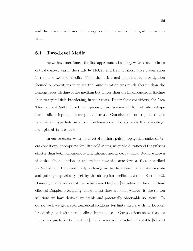
86

and then transformed into laboratory coordinates with a finite grid approxima-

tion.

6.1 Two-Level Media

As we have mentioned, the first appearance of solitary wave solutions in an

optical context was in the study by McCall and Hahn of short pulse propagation

in resonant two-level media. Their theoretical and experimental investigation

focused on conditions in which the pulse duration was much shorter than the

homogeneous lifetime of the medium but longer than the inhomogeneous lifetime

(due to crystal-field broadening, in their case). Under these conditions, the Area

Theorem and Self-Induced Transparency (see Section 2.2.10) actively reshape

non-idealized input pulse shapes and areas: Gaussian and other pulse shapes

tend toward hyperbolic secants, pulse breakup occurs, and areas that are integer

multiples of 2π are stable.

In our research, we are interested in short pulse propagation under differ-

ent conditions, appropriate for ultra-cold atoms, when the duration of the pulse is

shorter than both homogeneous and inhomogeneous decay times. We have shown

that the soliton solutions in this regime have the same form as those described

by McCall and Hahn with only a change in the definition of the distance scale

and pulse group velocity (set by the absorption coefficient κ), see Section 4.2.

However, the derivation of the pulse Area Theorem [36] relies on the smoothing

effect of Doppler broadening and we must show whether, without it, the soliton

solutions we have derived are stable and potentially observable solutions. To

do so, we have generated numerical solutions for finite media with no Doppler

broadening and with non-idealized input pulses. Our solutions show that, as

previously predicted by Lamb [53], the 2π-area soliton solution is stable [53] and

87

also that other pulse areas tend toward multiples of 2π, often with noticeable

pulse ringing.

For illustration, in Figure 6.1 we show the input and output pulse shapes

for two simulations for an absorbing medium 15 absorption depths long. The

medium is located in the shaded region of each graph. To simulate localized

pulses, we set the Rabi frequency equal to zero wherever Ωτ < 10−5 and ensure

that each pulse starts entirely outside the medium. In the top panel, we injected

a Gaussian-shaped pulse with area 2.1π. The output shows that pulse reshaping

does still occur in this regime, but there is a small amount of pulse ringing that

distorts the tails of the pulse. The final area of the output pulse is 1.995π. The

bottom panel shows results for a Gaussian input pulse with initial area equal to

the maximally unstable value 1.5π. As is reasonable, we see that pulse reshaping

is less effective and the amplitude of pulse ringing is more significant. The final

area in this case is 1.984π, remarkably close to 2π and showing that pulse area

continues to be a controlling parameter.

We therefore conclude that, even without Doppler broadening, the soliton

solution is relevant in finite-length two-level media for pulses with finite tails.

The reshaping effects, which are somewhat impeded by pulse ringing for large

deviations from the idealized solution, are not disruptive in practice. These

general conclusions also apply to three-level media.

6.2 Three-Level Media

The soliton solutions we derived for three-level media were significantly

more complicated than those associated with two-level media. It is important for

us to determine if the desired pulse-pulse dynamics of these solutions can sur-

vive under non-idealized conditions in finite media. Clader and Eberly [45, 50]

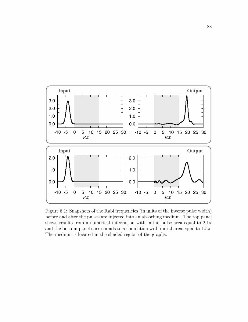
88

Input

0.0

1.0

2.0

3.0

-10 -5 0 5 10 15 20 25 30

-0.5

0

0.5

1.0

-10 -5 0 5 10 15 20 25 30

-0.5

0

0.5

1.0

-10 -5 0 5 10 15 20 25 30

OutputIn this document, I print the equation first in black and then in white (which

of course we can’t see on the white background)

Im(13) (1)

Im(23) (2)

x (3)

23 (4)

33 (5)

(6)

@

@x+

1

c

@

@t

= iµ12 (7)

@

@x+

1

c

@

@t

= iµ12 (8)

=

Z(x, t)dt (9)

=

Z(x, t)dt (10)

vg =c

1 + (11)

vg =c

1 + (12)

xpeak = ln

inj

13

inj23

(13)

xpeak = ln

inj

13

inj23

(14)

= µ/2 (15)

1

0.0

1.0

2.0

3.0

-10 -5 0 5 10 15 20 25 30

-0.5

0

0.5

1.0

-10 -5 0 5 10 15 20 25 30

-0.5

0

0.5

1.0

-10 -5 0 5 10 15 20 25 30

In this document, I print the equation first in black and then in white (whichof course we can’t see on the white background)

Im(13) (1)

Im(23) (2)

x (3)

23 (4)

33 (5)

(6)

@

@x+

1

c

@

@t

= iµ12 (7)

@

@x+

1

c

@

@t

= iµ12 (8)

=

Z(x, t)dt (9)

=

Z(x, t)dt (10)

vg =c

1 + (11)

vg =c

1 + (12)

xpeak = ln

inj

13

inj23

(13)

xpeak = ln

inj

13

inj23

(14)

= µ/2 (15)

1

Input

0.0

1.0

2.0

-10 -5 0 5 10 15 20 25 30

-0.5

0

0.5

1.0

-10 -5 0 5 10 15 20 25 30

-0.5

0

0.5

1.0

-10 -5 0 5 10 15 20 25 30

OutputIn this document, I print the equation first in black and then in white (which

of course we can’t see on the white background)

Im(13) (1)

Im(23) (2)

x (3)

23 (4)

33 (5)

(6)

@

@x+

1

c

@

@t

= iµ12 (7)

@

@x+

1

c

@

@t

= iµ12 (8)

=

Z(x, t)dt (9)

=

Z(x, t)dt (10)

vg =c

1 + (11)

vg =c

1 + (12)

xpeak = ln

inj

13

inj23

(13)

xpeak = ln

inj

13

inj23

(14)

= µ/2 (15)

1

In this document, I print the equation first in black and then in white (whichof course we can’t see on the white background)

Im(13) (1)

Im(23) (2)

x (3)

23 (4)

33 (5)

(6)

@

@x+

1

c

@

@t

= iµ12 (7)

@

@x+

1

c

@

@t

= iµ12 (8)

=

Z(x, t)dt (9)

=

Z(x, t)dt (10)

vg =c

1 + (11)

vg =c

1 + (12)

xpeak = ln

inj

13

inj23

(13)

xpeak = ln

inj

13

inj23

(14)

= µ/2 (15)

1

0.0

1.0

2.0

-10 -5 0 5 10 15 20 25 30

-0.5

0

0.5

1.0

-10 -5 0 5 10 15 20 25 30

-0.5

0

0.5

1.0

-10 -5 0 5 10 15 20 25 30

Figure 6.1: Snapshots of the Rabi frequencies (in units of the inverse pulse width)before and after the pulses are injected into an absorbing medium. The top panelshows results from a numerical integration with initial pulse area equal to 2.1πand the bottom panel corresponds to a simulation with initial area equal to 1.5π.The medium is located in the shaded region of the graphs.

89

probed the utility of their first-order two-pulse solutions extensively using numer-

ical solutions with a variety of media and pulse preparations. Their focus was

on conditions appropriate for room-temperature vapors with substantial Doppler

broadening so that non-hyperbolic secant pulses were reshaped and evolution was

guided by pulse area considerations.

Our present aim is to show that our second-order three-pulse soliton so-

lution has relevance in finite media with truncated pulses (without the infinitely

long tails of the analytic solution) without the stabilizing effects of Doppler broad-

ening and the Area Theorem. The conditions we explore here are important for

pulse propagation in ultra-cold atoms. To start, we present numerical results for

hyperbolic secant pulses to show how closely we can replicate results from our

second-order three-pulse soliton solution. We then deviate further from the ideal-

ized solution and find that, just as for two-level media, the overall behavior of the

soliton solution is retained but often with noticeable effects from pulse ringing. In

the simulations we present, the pulses are initially entirely outside the boundary

of the medium, with the field envelopes truncated at values below Ωτ < 10−5.

The medium in all cases is initially quiescent, with ρ11 = 1, ρ22 = ρ33 = 0.

6.2.1 Modeling High Bandwidth Pulse Storage and Memory Manip-ulation

Our second-order three-pulse soliton solution was derived for an infinitely

long medium and pulses with infinitely long tails. Fortunately, the solution it-

self provides the framework necessary to map the infinite analytic conditions to

initial conditions in finite media. The necessary control parameters can be ob-

tained by examining the analytic solution first in the asymptotic limit of large,

negative time. Then, the solution separates into the first-order one-pulse τb so-

lution propagating far behind (to the left) of the first-order two-pulse τa soliton

90

solution. In our second-order three-pulse soliton solution, we had to adjust the

integration constants carefully in order to observe a solution in which the pulse

storage/transfer process was effectively complete before the τb pulse reached the

imprint formed at ximp (recall Section 5.6). In a numerical or experimental set-

ting, this result is easily obtained by sufficiently delaying injection of the τb pulse;

the desired situation is sketched in Figure 6.2.

Control of storage locations is critically desirable. It has already been

observed [45, 49] that the time-matched τa pulses in the analytic solution are

related at any time by the ratio:

R(x) ≡∣∣∣∣Ωa

13(x, t)

Ωa23(x, t)

∣∣∣∣ = e−µτax/2+ηa12 , (6.1)

and we can use this formula to map the analytic solution at some position, x,

to initial conditions appropriate for numerical solutions in finite media. Suppose

that at x = 0, we inject time-matched pulses into a medium with initial ratio

R(0) ≡ R0 . Then, the formula above suggests that in a related analytic solution

R0 = eηa12 or ηa12 = lnR0. The signal (1-3) pulse in our soliton solution is stored

where ximp = ηa12/κ or, in terms of the ratio R0, we find ximp = lnR0. This

equation indicates that in finite media we can control the initial location of the

imprint by tuning the ratio of the injected τa pulses.

The initial pulse storage process from a specific simulation is shown in

Figure 6.3 for a medium 10 absorption depths long. At this stage of the sim-

ulation, we have injected the two hyperbolic secant pulses of duration τa, but

not yet the τb pulse. We injected a strong hyperbolic secant signal (1-3) pulse

with area 2π simultaneously with a weak hyperbolic secant control (2-3) pulse

with area 0.1π. The behavior of both pulses inside the medium clearly models

the initial behavior of our second-order three-pulse soliton solution; the τa signal

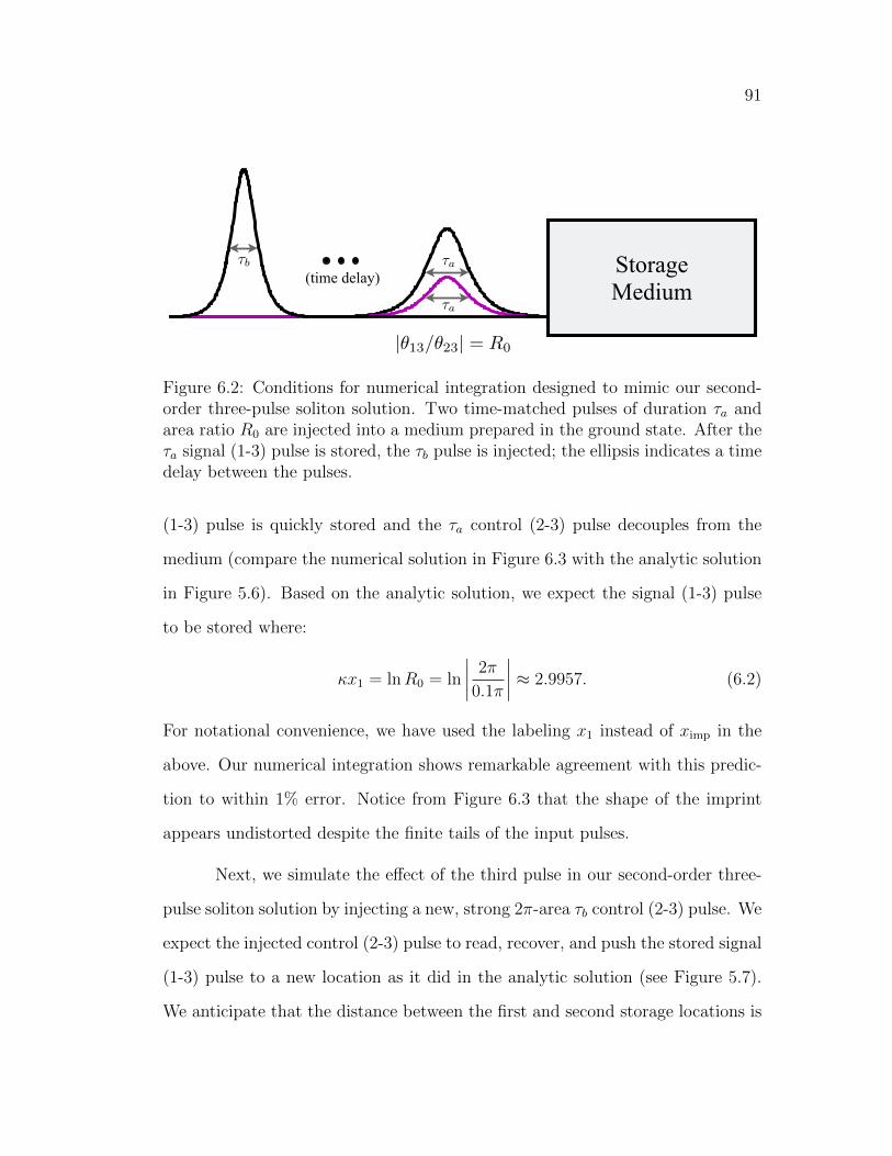
9113a (1)

x2 x1 = 3.560 (2)

t/a (3)

x1 = 3.000 (4)

a12 (5)

ln |R1| (6)

x1 = ln R + ab = (7)

|13/23| = R0 (8)

1/b (9)

(a12 + ab) (10)

a1 = 1, a2 = 5, a3 = i/5, (11)

a1 = 1, a2 = 5, a3 =1

5i, (12)

b1 = 0, b2 = 1, b3 = i, (13)

a = 2 b = 1, T = 25a, (14)

a1 = 1, a2 = 5, a3 =1

5i, (15)

b1 = 0, b2 = 1, b3 = i, (16)

a1 = 1 (17)

a2 = 2 (18)

aab13 (19)

↵x/2 (20)

! (21)

(22)

!3 (23)

!12 (24)

!23 (25)

1

b (1)

1/b (2)

a (3)

a1 = 1, a2 = 5, a3 = i/5, (4)

a1 = 1, a2 = 5, a3 =1

5i, (5)

b1 = 0, b2 = 1, b3 = i, (6)

a = 2 b = 1, T = 25a, (7)

a1 = 1, a2 = 5, a3 =1

5i, (8)

b1 = 0, b2 = 1, b3 = i, (9)

a1 = 1 (10)

a2 = 2 (11)

aab13 (12)

↵x/2 (13)

! (14)

(15)

!3 (16)

!12 (17)

!23 (18)

(19)

23 (20)

1 (21)

loc1 (22)

0.5 (23)

|131|2 (24)

1

Storage Medium

a (1)

1/b (2)

a (3)

a1 = 1, a2 = 5, a3 = i/5, (4)

a1 = 1, a2 = 5, a3 =1

5i, (5)

b1 = 0, b2 = 1, b3 = i, (6)

a = 2 b = 1, T = 25a, (7)

a1 = 1, a2 = 5, a3 =1

5i, (8)

b1 = 0, b2 = 1, b3 = i, (9)

a1 = 1 (10)

a2 = 2 (11)

aab13 (12)

↵x/2 (13)

! (14)

(15)

!3 (16)

!12 (17)

!23 (18)

(19)

23 (20)

1 (21)

loc1 (22)

0.5 (23)

|131|2 (24)

1

a (1)

1/b (2)

a (3)

a1 = 1, a2 = 5, a3 = i/5, (4)

a1 = 1, a2 = 5, a3 =1

5i, (5)

b1 = 0, b2 = 1, b3 = i, (6)

a = 2 b = 1, T = 25a, (7)

a1 = 1, a2 = 5, a3 =1

5i, (8)

b1 = 0, b2 = 1, b3 = i, (9)

a1 = 1 (10)

a2 = 2 (11)

aab13 (12)

↵x/2 (13)

! (14)

(15)

!3 (16)

!12 (17)

!23 (18)

(19)

23 (20)

1 (21)

loc1 (22)

0.5 (23)

|131|2 (24)

1

(time delay)

Figure 6.2: Conditions for numerical integration designed to mimic our second-order three-pulse soliton solution. Two time-matched pulses of duration τa andarea ratio R0 are injected into a medium prepared in the ground state. After theτa signal (1-3) pulse is stored, the τb pulse is injected; the ellipsis indicates a timedelay between the pulses.

(1-3) pulse is quickly stored and the τa control (2-3) pulse decouples from the

medium (compare the numerical solution in Figure 6.3 with the analytic solution

in Figure 5.6). Based on the analytic solution, we expect the signal (1-3) pulse

to be stored where:

κx1 = lnR0 = ln

∣∣∣∣2π

0.1π

∣∣∣∣ ≈ 2.9957. (6.2)

For notational convenience, we have used the labeling x1 instead of ximp in the

above. Our numerical integration shows remarkable agreement with this predic-

tion to within 1% error. Notice from Figure 6.3 that the shape of the imprint

appears undistorted despite the finite tails of the input pulses.

Next, we simulate the effect of the third pulse in our second-order three-

pulse soliton solution by injecting a new, strong 2π-area τb control (2-3) pulse. We

expect the injected control (2-3) pulse to read, recover, and push the stored signal

(1-3) pulse to a new location as it did in the analytic solution (see Figure 5.7).

We anticipate that the distance between the first and second storage locations is

92

x1 = 3.0 (1)

(x, t0) (2)

22 (3)

x = 0 (4)

ln R00 (5)

13a (6)

x2 = (7)

t/a (8)

x2 = 6.5600 (9)

x2 = x1 + ab = 6.6593 (10)

a12 (11)

ln |R1| (12)

x1 = ln R0 = 3.0000 (13)

|13/23| = R00 (14)

1/b (15)

(a12 + ab) (16)

a1 = 1, a2 = 5, a3 = i/5, (17)

a1 = 1, a2 = 5, a3 =1

5i, (18)

b1 = 0, b2 = 1, b3 = i, (19)

a = 2 b = 1, T = 25a, (20)

a1 = 1, a2 = 5, a3 =1

5i, (21)

b1 = 0, b2 = 1, b3 = i, (22)

a1 = 1 (23)

a2 = 2 (24)

aab13 (25)

1

x = 0 (1)

ln R00 (2)

13a (3)

x2 x1 = 3.560 (4)

t/a (5)

x1 = 3.000 (6)

a12 (7)

ln |R1| (8)

x1 = ln R0 = 2.9957 (9)

|13/23| = R00 (10)

1/b (11)

(a12 + ab) (12)

a1 = 1, a2 = 5, a3 = i/5, (13)

a1 = 1, a2 = 5, a3 =1

5i, (14)

b1 = 0, b2 = 1, b3 = i, (15)

a = 2 b = 1, T = 25a, (16)

a1 = 1, a2 = 5, a3 =1

5i, (17)

b1 = 0, b2 = 1, b3 = i, (18)

a1 = 1 (19)

a2 = 2 (20)

aab13 (21)

↵x/2 (22)

! (23)

(24)

!3 (25)

1

|13a|2 (1)

t/a (2)

x1 = ln R = 2.997 (3)

a12 (4)

ln |R1| (5)

x1 = ln R + ab = (6)

13/23 = |R1| (7)

1/b (8)

(a12 + ab) (9)

a1 = 1, a2 = 5, a3 = i/5, (10)

a1 = 1, a2 = 5, a3 =1

5i, (11)

b1 = 0, b2 = 1, b3 = i, (12)

a = 2 b = 1, T = 25a, (13)

a1 = 1, a2 = 5, a3 =1

5i, (14)

b1 = 0, b2 = 1, b3 = i, (15)

a1 = 1 (16)

a2 = 2 (17)

aab13 (18)

↵x/2 (19)

! (20)

(21)

!3 (22)

!12 (23)

!23 (24)

(25)

1

|13a|2 (1)

t/a (2)

x1 = ln R = 2.997 (3)

a12 (4)

ln |R1| (5)

x1 = ln R + ab = (6)

13/23 = |R1| (7)

1/b (8)

(a12 + ab) (9)

a1 = 1, a2 = 5, a3 = i/5, (10)

a1 = 1, a2 = 5, a3 =1

5i, (11)

b1 = 0, b2 = 1, b3 = i, (12)

a = 2 b = 1, T = 25a, (13)

a1 = 1, a2 = 5, a3 =1

5i, (14)

b1 = 0, b2 = 1, b3 = i, (15)

a1 = 1 (16)

a2 = 2 (17)

aab13 (18)

↵x/2 (19)

! (20)

(21)

!3 (22)

!12 (23)

!23 (24)

(25)

1

0 205 150

10

2

4

6

8

In this document, I print the equation first in black and then in white (whichof course we can’t see on the white background)

Im(13) (1)

Im(23) (2)

x (3)

23 (4)

33 (5)

(6)

@

@x+

1

c

@

@t

= iµ12 (7)

@

@x+

1

c

@

@t

= iµ12 (8)

=

Z(x, t)dt (9)

=

Z(x, t)dt (10)

vg =c

1 + (11)

vg =c

1 + (12)

xpeak = ln

inj

13

inj23

(13)

xpeak = ln

inj

13

inj23

(14)

= µ/2 (15)

1

10

108642

In this document, I print the equation first in black and then in white (whichof course we can’t see on the white background)

Im(13) (1)

Im(23) (2)

x (3)

23 (4)

33 (5)

(6)

@

@x+

1

c

@

@t

= iµ12 (7)

@

@x+

1

c

@

@t

= iµ12 (8)

=

Z(x, t)dt (9)

=

Z(x, t)dt (10)

vg =c

1 + (11)

vg =c

1 + (12)

xpeak = ln

inj

13

inj23

(13)

xpeak = ln

inj

13

inj23

(14)

= µ/2 (15)

1

In this document, I print the equation first in black and then in white (whichof course we can’t see on the white background)

(1)

Im(13) (2)

Im(23) (3)

x (4)

t

s(5)

t/s (6)

23 (7)

33 (8)

(9)

@

@x+

1

c

@

@t

= iµ12 (10)

@

@x+

1

c

@

@t

= iµ12 (11)

=

Z(x, t)dt (12)

=

Z(x, t)dt (13)

vg =c

1 + (14)

vg =c

1 + (15)

xpeak = ln

inj

13

inj23

(16)

xpeak = ln

inj

13

inj23

(17)

1

0

Pulse Areas

2

Signal Pulse

1

4

3

In this document, I print the equation first in black and then in white (whichof course we can’t see on the white background)

loc1 (1)

1.5 (2)

|13s|2 (3)

Im(13) (4)

Im(23) (5)

x (6)

t

s(7)

t/s (8)

23 (9)

33 (10)

(11)

@

@x+

1

c

@

@t

= iµ12 (12)

@

@x+

1

c

@

@t

= iµ12 (13)

=

Z(x, t)dt (14)

=

Z(x, t)dt (15)

vg =c

1 + (16)

vg =c

1 + (17)

xpeak = ln

inj

13

inj23

(18)

1

In this document, I print the equation first in black and then in white (whichof course we can’t see on the white background)

loc1 (1)

2 (2)

|13s|2 (3)

Im(13) (4)

Im(23) (5)

x (6)

t

s(7)

t/s (8)

23 (9)

33 (10)

(11)

@

@x+

1

c

@

@t

= iµ12 (12)

@

@x+

1

c

@

@t

= iµ12 (13)

=

Z(x, t)dt (14)

=

Z(x, t)dt (15)

vg =c

1 + (16)

vg =c

1 + (17)

xpeak = ln

inj

13

inj23

(18)

1

In this document, I print the equation first in black and then in white (whichof course we can’t see on the white background)

loc1 (1)

0.5 (2)

|13s|2 (3)

Im(13) (4)

Im(23) (5)

x (6)

t

s(7)

t/s (8)

23 (9)

33 (10)

(11)

@

@x+

1

c

@

@t

= iµ12 (12)

@

@x+

1

c

@

@t

= iµ12 (13)

=

Z(x, t)dt (14)

=

Z(x, t)dt (15)

vg =c

1 + (16)

vg =c

1 + (17)

xpeak = ln

inj

13

inj23

(18)

1

In this document, I print the equation first in black and then in white (whichof course we can’t see on the white background)

23 (1)

x1 (2)

1 (3)

loc1 (4)

0.5 (5)

|131|2 (6)

Im(13) (7)

Im(23) (8)

x (9)

t

1(10)

t/1 (11)

23 (12)

33 (13)

(14)

@

@x+

1

c

@

@t

= iµ12 (15)

@

@x+

1

c

@

@t

= iµ12 (16)

=

Z(x, t)dt (17)

=

Z(x, t)dt (18)

vg =c

1 + (19)

1

Stored Signal Pulse Imprint

Analytic Prediction:Numerical Result:

5

Before After

-1.6

-0.8

0

0.8

1.6

-10 -5 0 5 10 15 20

-0.5

0

0.5

1.0

-10 -5 0 5 10 15 20

-1.6

-0.8

0

0.8

1.6

-10 -5 0 5 10 15 20

-0.5

0

0.5

1.0

-10 -5 0 5 10 15 20

-1.6

-0.8

0

0.8

1.6

-10 -5 0 5 10 15 20

-0.5

0

0.5

1.0

-10 -5 0 5 10 15 20x (34)

=

11 12

21 22

(35)

=

11 12

21 22

(36)

H = h

2

0@

0 0 13

0 0 23

13 23 0

1A (37)

H = h

2

0@

0 0 13

0 0 23

13 23 0

1A (38)

H = h

2

0

13

13 0

(39)

H = h

2

0

0

(40)

H = h

2

0

0

(41)

ih@

@t= [H, ] (42)

ih@

@t= [H, ] (43)

@

@x+

1

c

@

@t

13 = iµ1313 (44)

@

@x+

1

c

@

@t

13 = iµ2323 (45)

@

@x+

1

c

@

@t

23 = iµ1313 (46)

@

@x+

1

c

@

@t

23 = iµ2323 (47)

3

x (34)

=

11 12

21 22

(35)

=

11 12

21 22

(36)

H = h

2

0@

0 0 13

0 0 23

13 23 0

1A (37)

H = h

2

0@

0 0 13

0 0 23

13 23 0

1A (38)

H = h

2

0

13

13 0

(39)

H = h

2

0

0

(40)

H = h

2

0

0

(41)

ih@

@t= [H, ] (42)

ih@

@t= [H, ] (43)

@

@x+

1

c

@

@t

13 = iµ1313 (44)

@

@x+

1

c

@

@t

13 = iµ2323 (45)

@

@x+

1

c

@

@t

23 = iµ1313 (46)

@

@x+

1

c

@

@t

23 = iµ2323 (47)

3

x (34)

=

11 12

21 22

(35)

=

11 12

21 22

(36)

H = h

2

0@

0 0 13

0 0 23

13 23 0

1A (37)

H = h

2

0@

0 0 13

0 0 23

13 23 0

1A (38)

H = h

2

0

13

13 0

(39)

H = h

2

0

0

(40)

H = h

2

0

0

(41)

ih@

@t= [H, ] (42)

ih@

@t= [H, ] (43)

@

@x+

1

c

@

@t

13 = iµ1313 (44)

@

@x+

1

c

@

@t

13 = iµ2323 (45)

@

@x+

1

c

@

@t

23 = iµ1313 (46)

@

@x+

1

c

@

@t

23 = iµ2323 (47)

3

x (34)

=

11 12

21 22

(35)

=

11 12

21 22

(36)

H = h

2

0@

0 0 13

0 0 23

13 23 0

1A (37)

H = h

2

0@

0 0 13

0 0 23

13 23 0

1A (38)

H = h

2

0

13

13 0

(39)

H = h

2

0

0

(40)

H = h

2

0

0

(41)

ih@

@t= [H, ] (42)

ih@

@t= [H, ] (43)

@

@x+

1

c

@

@t

13 = iµ1313 (44)

@

@x+

1

c

@

@t

13 = iµ2323 (45)

@

@x+

1

c

@

@t

23 = iµ1313 (46)

@

@x+

1

c

@

@t

23 = iµ2323 (47)

3

x (34)

=

11 12

21 22

(35)

=

11 12

21 22

(36)

H = h

2

0@

0 0 13

0 0 23

13 23 0

1A (37)

H = h

2

0@

0 0 13

0 0 23

13 23 0

1A (38)

H = h

2

0

13

13 0

(39)

H = h

2

0

0

(40)

H = h

2

0

0

(41)

ih@

@t= [H, ] (42)

ih@

@t= [H, ] (43)

@

@x+

1

c

@

@t

13 = iµ1313 (44)

@

@x+

1

c

@

@t

13 = iµ2323 (45)

@

@x+

1

c

@

@t

23 = iµ1313 (46)

@

@x+

1

c

@

@t

23 = iµ2323 (47)

3

x (34)

=

11 12

21 22

(35)

=

11 12

21 22

(36)

H = h

2

0@

0 0 13

0 0 23

13 23 0

1A (37)

H = h

2

0@

0 0 13

0 0 23

13 23 0

1A (38)

H = h

2

0

13

13 0

(39)

H = h

2

0

0

(40)

H = h

2

0

0

(41)

ih@

@t= [H, ] (42)

ih@

@t= [H, ] (43)

@

@x+

1

c

@

@t

13 = iµ1313 (44)

@

@x+

1

c

@

@t

13 = iµ2323 (45)

@

@x+

1

c

@

@t

23 = iµ1313 (46)

@

@x+

1

c

@

@t

23 = iµ2323 (47)

3

xpeak = lninj

13 /inj23

(14)

xpeak = lninj

13 /inj23

(15)

= 0.9 storage (16)

storage (17)

storage (18)

control (19)

control (20)

xmove = ln

storage control

storage + control

(21)

xmove = ln

storage control

storage + control

(22)

x (23)

=

11 12

21 22

(24)

=

11 12

21 22

(25)

H = h

2

0@

0 0 13

0 0 23

13 23 0

1A (26)

H = h

2

0@

0 0 13

0 0 23

13 23 0

1A (27)

H = h

2

0

13

13 0

(28)

2

xpeak = lninj

13 /inj23

(14)

xpeak = lninj

13 /inj23

(15)

= 0.9 storage (16)

storage (17)

storage (18)

control (19)

control (20)

xmove = ln

storage control

storage + control

(21)

xmove = ln

storage control

storage + control

(22)

x (23)

=

11 12

21 22

(24)

=

11 12

21 22

(25)

H = h

2

0@

0 0 13

0 0 23

13 23 0

1A (26)

H = h

2

0@

0 0 13

0 0 23

13 23 0

1A (27)

H = h

2

0

13

13 0

(28)

2

= µs/2 (14)

xpeak = lninj

13 /inj23

(15)

xpeak = lninj

13 /inj23

(16)

= 0.9 storage (17)

storage (18)

storage (19)

control (20)

control (21)

xmove = ln

storage control

storage + control

(22)

xmove = ln

storage control

storage + control

(23)

x (24)

=

11 12

21 22

(25)

=

11 12

21 22

(26)

H = h

2

0@

0 0 13

0 0 23

13 23 0

1A (27)

H = h

2

0@

0 0 13

0 0 23

13 23 0

1A (28)

2

-1.6

-0.8

0

0.8

1.6

-10 -5 0 5 10 15 20

-0.5

0

0.5

1.0

-10 -5 0 5 10 15 20

-1.6

-0.8

0

0.8

1.6

-10 -5 0 5 10 15 20

-0.5

0

0.5

1.0

-10 -5 0 5 10 15 20

In this document, I print the equation first in black and then in white (whichof course we can’t see on the white background)

Im(13) (1)

23 (2)

33 (3)

(4)

@

@x+

1

c

@

@t

= iµ12 (5)

@

@x+

1

c

@

@t

= iµ12 (6)

=

(x, t)dt (7)

=

(x, t)dt (8)

vg =c

1 + (9)

vg =c

1 + (10)

xpeak = ln

inj

13

inj23

(11)

xpeak = ln

inj

13

inj23

(12)

= µ/2 (13)

= µ/2 (14)

1

In this document, I print the equation first in black and then in white (whichof course we can’t see on the white background)

Im(13) (1)

Im(23) (2)

23 (3)

33 (4)

(5)

@

@x+

1

c

@

@t

= iµ12 (6)

@

@x+

1

c

@

@t

= iµ12 (7)

=

(x, t)dt (8)

=

(x, t)dt (9)

vg =c

1 + (10)

vg =c

1 + (11)

xpeak = ln

inj

13

inj23

(12)

xpeak = ln

inj

13

inj23

(13)

= µ/2 (14)

= µ/2 (15)

1

In this document, I print the equation first in black and then in white (whichof course we can’t see on the white background)

Im(13) (1)

Im(23) (2)

23 (3)

33 (4)

(5)

@

@x+

1

c

@

@t

= iµ12 (6)

@

@x+

1

c

@

@t

= iµ12 (7)

=

(x, t)dt (8)

=

(x, t)dt (9)

vg =c

1 + (10)

vg =c

1 + (11)

xpeak = ln

inj

13

inj23

(12)

xpeak = ln

inj

13

inj23

(13)

= µ/2 (14)

= µ/2 (15)

1

-1.6

-0.8

0

0.8

1.6

-10 -5 0 5 10 15 20

-0.5

0

0.5

1.0

-10 -5 0 5 10 15 20

x (34)

=

11 12

21 22

(35)

=

11 12

21 22

(36)

H = h

2

0@

0 0 13

0 0 23

13 23 0

1A (37)

H = h

2

0@

0 0 13

0 0 23

13 23 0

1A (38)

H = h

2

0

13

13 0

(39)

H = h

2

0

0

(40)

H = h

2

0

0

(41)

ih@

@t= [H, ] (42)

ih@

@t= [H, ] (43)

@

@x+

1

c

@

@t

13 = iµ1313 (44)

@

@x+

1

c

@

@t

13 = iµ2323 (45)

@

@x+

1

c

@

@t

23 = iµ1313 (46)

@

@x+

1

c

@

@t

23 = iµ2323 (47)

3

In this document, I print the equation first in black and then in white (whichof course we can’t see on the white background)

23 (1)

1 (2)

loc1 (3)

0.5 (4)

|131|2 (5)

Im(13) (6)

Im(23) (7)

x (8)

t

1(9)

t/1 (10)

23 (11)

33 (12)

(13)

@

@x+

1

c

@

@t

= iµ12 (14)

@

@x+

1

c

@

@t

= iµ12 (15)

=

(x, t)dt (16)

=

(x, t)dt (17)

vg =c

1 + (18)

vg =c

1 + (19)

1

-1.6

-0.8

0

0.8

1.6

-10 -5 0 5 10 15 20

-0.5

0

0.5

1.0

-10 -5 0 5 10 15 20

Step 2

FIG. 3: Manipulation of the memory location. Pulse Rabi frequencies (top) and atomic density matrix elements (bottom) atthree distinct times: before the second control pulse is injected (left), while the imprint is being relocated (middle), and afterthe signal pulse information has been moved and the control field has exited the medium (right). The medium is located inthe shaded region of each plot.

In this document, I print the equation first in black and then in white (whichof course we can’t see on the white background)

23 (1)

1 (2)

loc1 (3)

0.5 (4)

|131|2 (5)

Im(13) (6)

Im(23) (7)

x (8)

t

1(9)

t/1 (10)

23 (11)

33 (12)

(13)

@

@x+

1

c

@

@t

= iµ12 (14)

@

@x+

1

c

@

@t

= iµ12 (15)

=

(x, t)dt (16)

=

(x, t)dt (17)

vg =c

1 + (18)

vg =c

1 + (19)

1

10

In this document, I print the equation first in black and then in white (whichof course we can’t see on the white background)

1 (1)

loc1 (2)

0.5 (3)

|131|2 (4)

Im(13) (5)

Im(23) (6)

x (7)

t

1(8)

t/1 (9)

23 (10)

33 (11)

(12)

@

@x+

1

c

@

@t

= iµ12 (13)

@

@x+

1

c

@

@t

= iµ12 (14)

=

(x, t)dt (15)

=

(x, t)dt (16)

vg =c

1 + (17)

vg =c

1 + (18)

xpeak = ln

inj

13

inj23

(19)

1

0 205 150

10

2

4

6

8

In this document, I print the equation first in black and then in white (whichof course we can’t see on the white background)

Im(13) (1)

Im(23) (2)

x (3)

23 (4)

33 (5)

(6)

@

@x+

1

c

@

@t

= iµ12 (7)

@

@x+

1

c

@

@t

= iµ12 (8)

=

(x, t)dt (9)

=

(x, t)dt (10)

vg =c

1 + (11)

vg =c

1 + (12)

xpeak = ln

inj

13

inj23

(13)

xpeak = ln

inj

13

inj23

(14)

= µ/2 (15)

1

Step 2

10

8642

In this document, I print the equation first in black and then in white (whichof course we can’t see on the white background)

Im(13) (1)

Im(23) (2)

x (3)

23 (4)

33 (5)

(6)

@

@x+

1

c

@

@t

= iµ12 (7)

@

@x+

1

c

@

@t

= iµ12 (8)

=

(x, t)dt (9)

=

(x, t)dt (10)

vg =c

1 + (11)

vg =c

1 + (12)

xpeak = ln

inj

13

inj23

(13)

xpeak = ln

inj

13

inj23

(14)

= µ/2 (15)

1

In this document, I print the equation first in black and then in white (whichof course we can’t see on the white background)

(1)

Im(13) (2)

Im(23) (3)

x (4)

t

s(5)

t/s (6)

23 (7)

33 (8)

(9)

@

@x+

1

c

@

@t

= iµ12 (10)

@

@x+

1

c

@

@t

= iµ12 (11)

=

(x, t)dt (12)

=

(x, t)dt (13)

vg =c

1 + (14)

vg =c

1 + (15)

xpeak = ln

inj

13

inj23

(16)

xpeak = ln

inj

13

inj23

(17)

1

0

Pulse Areas (absolute values)

2

1

4

3

In this document, I print the equation first in black and then in white (whichof course we can’t see on the white background)

loc1 (1)

1.5 (2)

|13s|2 (3)

Im(13) (4)

Im(23) (5)

x (6)

t

s(7)

t/s (8)

23 (9)

33 (10)

(11)

@

@x+

1

c

@

@t

= iµ12 (12)

@

@x+

1

c

@

@t

= iµ12 (13)

=

(x, t)dt (14)

=

(x, t)dt (15)

vg =c

1 + (16)

vg =c

1 + (17)

xpeak = ln

inj

13

inj23

(18)

1

In this document, I print the equation first in black and then in white (whichof course we can’t see on the white background)

loc1 (1)

2 (2)

|13s|2 (3)

Im(13) (4)

Im(23) (5)

x (6)

t

s(7)

t/s (8)

23 (9)

33 (10)

(11)

@

@x+

1

c

@

@t

= iµ12 (12)

@

@x+

1

c

@

@t

= iµ12 (13)

=

(x, t)dt (14)

=

(x, t)dt (15)

vg =c

1 + (16)

vg =c

1 + (17)

xpeak = ln

inj

13

inj23

(18)

1

In this document, I print the equation first in black and then in white (whichof course we can’t see on the white background)

loc1 (1)

0.5 (2)

|13s|2 (3)

Im(13) (4)

Im(23) (5)

x (6)

t

s(7)

t/s (8)

23 (9)

33 (10)

(11)

@

@x+

1

c

@

@t

= iµ12 (12)

@

@x+

1

c

@

@t

= iµ12 (13)

=

(x, t)dt (14)

=

(x, t)dt (15)

vg =c

1 + (16)

vg =c

1 + (17)

xpeak = ln

inj

13

inj23

(18)

1

Signal pulse In this document, I print the equation first in black and then in white (which

of course we can’t see on the white background)

23 (1)

x1 (2)

1 (3)

loc1 (4)

0.5 (5)

|131|2 (6)

Im(13) (7)

Im(23) (8)

x (9)

t

1(10)

t/1 (11)

23 (12)

33 (13)

(14)

@

@x+

1

c

@

@t

= iµ12 (15)

@

@x+

1

c

@

@t

= iµ12 (16)

=

(x, t)dt (17)

=

(x, t)dt (18)

vg =c

1 + (19)

1

In this document, I print the equation first in black and then in white (whichof course we can’t see on the white background)

23 (1)

x1 (2)

x2 (3)

1 (4)

loc1 (5)

0.5 (6)

|131|2 (7)

Im(13) (8)

Im(23) (9)

x (10)

t

1(11)

t/1 (12)

23 (13)

33 (14)

(15)

@

@x+

1

c

@

@t

= iµ12 (16)

@

@x+

1

c

@

@t

= iµ12 (17)

=

(x, t)dt (18)

=

(x, t)dt (19)

vg =c

1 + (20)

1

FIG. 4: Evolution of the signal pulse during the memory ma-nipulation step. Absolute values of the signal (black) andcontrol (purple) pulse areas are shown in the inset. The pulseareas are equal at the initial and final storage locations, la-beled x1 and x2, respectively, in the figure.

demonstrate a three-step procedure of optical pulse stor-age, memory manipulation, and retrieval. The ratio ofthe input signal and control pulse areas determine wherethe signal pulse is initially stored and our simulationsshow that we can reliably move or retrieve the storedpulse on-demand by manipulating the width of subse-quent control pulses.

There are several important features of optical controlin the short-pulse regime to note. First, the resonantinteraction allows for very ecient atom-field couplingand high fidelity pulse storage and retrieval. Second, inthe absence of adiabatic or quasi-steady state conditions

In this document, I print the equation first in black and then in white (whichof course we can’t see on the white background)

1 (1)

loc1 (2)

0.5 (3)

|131|2 (4)

Im(13) (5)

Im(23) (6)

x (7)

t

1(8)

t/1 (9)

23 (10)

33 (11)

(12)

@

@x+

1

c

@

@t

= iµ12 (13)

@

@x+

1

c

@

@t

= iµ12 (14)

=

(x, t)dt (15)

=

(x, t)dt (16)

vg =c

1 + (17)

vg =c

1 + (18)

xpeak = ln

inj

13

inj23

(19)

1

0 205 150

10

2

4

6

8

In this document, I print the equation first in black and then in white (whichof course we can’t see on the white background)

Im(13) (1)

Im(23) (2)

x (3)

23 (4)

33 (5)

(6)

@

@x+

1

c

@

@t

= iµ12 (7)

@

@x+

1

c

@

@t

= iµ12 (8)

=

(x, t)dt (9)

=

(x, t)dt (10)

vg =c

1 + (11)

vg =c

1 + (12)

xpeak = ln

inj

13

inj23

(13)

xpeak = ln

inj

13

inj23

(14)

= µ/2 (15)

1

10

2

1

4

3

Signal pulse Step 3

In this document, I print the equation first in black and then in white (whichof course we can’t see on the white background)

Im(13) (1)

Im(23) (2)

x (3)

23 (4)

33 (5)

(6)

@

@x+

1

c

@

@t

= iµ12 (7)

@

@x+

1

c

@

@t

= iµ12 (8)

=

(x, t)dt (9)

=

(x, t)dt (10)

vg =c

1 + (11)

vg =c

1 + (12)

xpeak = ln

inj

13

inj23

(13)

xpeak = ln

inj

13

inj23

(14)

= µ/2 (15)

1

108642

In this document, I print the equation first in black and then in white (whichof course we can’t see on the white background)

(1)

Im(13) (2)

Im(23) (3)

x (4)

t

s(5)

t/s (6)

23 (7)

33 (8)

(9)

@

@x+

1

c

@

@t

= iµ12 (10)

@

@x+

1

c

@

@t

= iµ12 (11)

=

(x, t)dt (12)

=

(x, t)dt (13)

vg =c

1 + (14)

vg =c

1 + (15)

xpeak = ln

inj

13

inj23

(16)

xpeak = ln

inj

13

inj23

(17)

1

0

Pulse Areas

In this document, I print the equation first in black and then in white (whichof course we can’t see on the white background)

loc1 (1)

1.5 (2)

|13s|2 (3)

Im(13) (4)

Im(23) (5)

x (6)

t

s(7)

t/s (8)

23 (9)

33 (10)

(11)

@

@x+

1

c

@

@t

= iµ12 (12)

@

@x+

1

c

@

@t

= iµ12 (13)

=

(x, t)dt (14)

=

(x, t)dt (15)

vg =c

1 + (16)

vg =c

1 + (17)

xpeak = ln

inj

13

inj23

(18)

1

In this document, I print the equation first in black and then in white (whichof course we can’t see on the white background)

loc1 (1)

2 (2)

|13s|2 (3)

Im(13) (4)

Im(23) (5)

x (6)

t

s(7)

t/s (8)

23 (9)

33 (10)

(11)

@

@x+

1

c

@

@t

= iµ12 (12)

@

@x+

1

c

@

@t

= iµ12 (13)

=

(x, t)dt (14)

=

(x, t)dt (15)

vg =c

1 + (16)

vg =c

1 + (17)

xpeak = ln

inj

13

inj23

(18)

1

In this document, I print the equation first in black and then in white (whichof course we can’t see on the white background)

loc1 (1)

0.5 (2)

|13s|2 (3)

Im(13) (4)

Im(23) (5)

x (6)

t

s(7)

t/s (8)

23 (9)

33 (10)

(11)

@

@x+

1

c

@

@t

= iµ12 (12)

@

@x+

1

c

@

@t

= iµ12 (13)

=

(x, t)dt (14)

=

(x, t)dt (15)

vg =c

1 + (16)

vg =c

1 + (17)

xpeak = ln

inj

13

inj23

(18)

1

In this document, I print the equation first in black and then in white (whichof course we can’t see on the white background)

23 (1)

x1 (2)

x2 (3)

1 (4)

loc1 (5)

0.5 (6)

|131|2 (7)

Im(13) (8)

Im(23) (9)

x (10)

t

1(11)

t/1 (12)

23 (13)

33 (14)

(15)

@

@x+

1

c

@

@t

= iµ12 (16)

@

@x+

1

c

@

@t

= iµ12 (17)

=

(x, t)dt (18)

=

(x, t)dt (19)

vg =c

1 + (20)

1

In this document, I print the equation first in black and then in white (whichof course we can’t see on the white background)

23 (1)

1 (2)

loc1 (3)

0.5 (4)

|131|2 (5)

Im(13) (6)

Im(23) (7)

x (8)

t

1(9)

t/1 (10)

23 (11)

33 (12)

(13)

@

@x+

1

c

@

@t

= iµ12 (14)

@

@x+

1

c

@

@t

= iµ12 (15)

=

(x, t)dt (16)

=

(x, t)dt (17)

vg =c

1 + (18)

vg =c

1 + (19)

1

FIG. 5: signal pulse retrieval. The square of the recoveredsignal pulse Rabi frequency is shown at distinct locations inthe medium. The signal (black) and control (purple) pulseareas are plotted in the inset.

there is no requirement that the control field is strong andthe signal pulse weak. In fact, in the first step of our stor-age and re-storage procedure the opposite occurs, it is theprobe pulse that is strong while the control pulse is weak.Third, when the signal field ultimately emerges from themedium the control pulse is o↵ or extremely weak, sothat separating the probe and control beams would poselittle problem, despite the co-propagating geometry. Fi-nally, we note that if no control field is injected in stepone, then the Self-Induced Transparency (SIT) [24] typesignal field is slowed, but ultimately transmitted. This

xpeak = lninj

13 /inj23

(14)

xpeak = lninj

13 /inj23

(15)

= 0.9 storage (16)

storage (17)

storage (18)

control (19)

control (20)

xmove = ln

storage control

storage + control

(21)

xmove = ln

storage control

storage + control

(22)

x (23)

=

11 12

21 22

(24)

=

11 12

21 22

(25)

H = h

2

0@

0 0 13

0 0 23

13 23 0

1A (26)

H = h

2

0@

0 0 13

0 0 23

13 23 0

1A (27)

H = h

2

0

13

13 0

(28)

2

xpeak = lninj

13 /inj23

(14)

xpeak = lninj

13 /inj23

(15)

= 0.9 storage (16)

storage (17)

storage (18)

control (19)

control (20)

xmove = ln

storage control

storage + control

(21)

xmove = ln

storage control

storage + control

(22)

x (23)

=

11 12

21 22

(24)

=

11 12

21 22

(25)

H = h

2

0@

0 0 13

0 0 23

13 23 0

1A (26)

H = h

2

0@

0 0 13

0 0 23

13 23 0

1A (27)

H = h

2

0

13

13 0

(28)

2

= µs/2 (14)

xpeak = lninj

13 /inj23

(15)

xpeak = lninj

13 /inj23

(16)

= 0.9 storage (17)

storage (18)

storage (19)

control (20)

control (21)

xmove = ln

storage control

storage + control

(22)

xmove = ln

storage control

storage + control

(23)

x (24)

=

11 12

21 22

(25)

=

11 12

21 22

(26)

H = h

2

0@

0 0 13

0 0 23

13 23 0

1A (27)

H = h

2

0@

0 0 13

0 0 23

13 23 0

1A (28)

2

-1.6

-0.8

0

0.8

1.6

-10 -5 0 5 10 15 20

-0.5

0

0.5

1.0

-10 -5 0 5 10 15 20

-1.6

-0.8

0

0.8

1.6

-10 -5 0 5 10 15 20

-0.5

0

0.5

1.0

-10 -5 0 5 10 15 20

In this document, I print the equation first in black and then in white (whichof course we can’t see on the white background)

Im(13) (1)

23 (2)

33 (3)

(4)

@

@x+

1

c

@

@t

= iµ12 (5)

@

@x+

1

c

@

@t

= iµ12 (6)

=

Z(x, t)dt (7)

=

Z(x, t)dt (8)

vg =c

1 + (9)

vg =c

1 + (10)

xpeak = ln

inj

13

inj23

(11)

xpeak = ln

inj

13

inj23

(12)

= µ/2 (13)

= µ/2 (14)

1

In this document, I print the equation first in black and then in white (whichof course we can’t see on the white background)

Im(13) (1)

Im(23) (2)

23 (3)

33 (4)

(5)

@

@x+

1

c

@

@t

= iµ12 (6)

@

@x+

1

c

@

@t

= iµ12 (7)

=

Z(x, t)dt (8)

=

Z(x, t)dt (9)

vg =c

1 + (10)

vg =c

1 + (11)

xpeak = ln

inj

13

inj23

(12)

xpeak = ln

inj

13

inj23

(13)

= µ/2 (14)

= µ/2 (15)

1

In this document, I print the equation first in black and then in white (whichof course we can’t see on the white background)

Im(13) (1)

Im(23) (2)

23 (3)

33 (4)

(5)

@

@x+

1

c

@

@t

= iµ12 (6)

@

@x+

1

c

@

@t

= iµ12 (7)

=

Z(x, t)dt (8)

=

Z(x, t)dt (9)

vg =c

1 + (10)

vg =c

1 + (11)

xpeak = ln

inj

13

inj23

(12)

xpeak = ln

inj

13

inj23

(13)

= µ/2 (14)

= µ/2 (15)

1

Figure 6.3: Results of a numerical integration of the three-level Maxwell-Blochequations. The medium is located between κx = 0 and κx = 10. Depletion ofthe initially strong 2π-area signal (1-3) pulse is shown on the left. The areas ofboth τa pulses are shown in the inset and the areas are equal where κx1 ≈ 3.The graph on the right shows a snapshot of the stored pulse imprint after theamplified τa control (2-3) pulse has exited the medium.

controlled by the phase lag:

κx2 − κx1 = δab =

(τa + τbτa − τb

). (6.3)

By tuning the duration of the τb control (2-3) pulse we should therefore be able

to choose where to deposit the imprint. We want to re-imprint the signal (1-3)

pulse at a location well within the boundary of the medium to minimize loss of

its information. We therefore carefully select τb = 0.95τa so that δab = 3.6636

and we anticipate the signal (1-3) pulse to be re-imprinted where:

κx2 = κx1 + δab = 2.9957 + 3.6636 = 6.6593. (6.4)

The results of our numerical integration are shown in Figure 6.4.

The figure shows that the medium responds as predicted (note locations

of finite atomic coherence ρ12), but with a slight excitation remaining on the

signal (1-3) pulse transition frequency co-propagating with the control (2-3) pulse

93

Before After

-1.6

-0.8

0

0.8

1.6

-10 -5 0 5 10 15 20

-0.5

0

0.5

1.0

-10 -5 0 5 10 15 20

-1.6

-0.8

0

0.8

1.6

-10 -5 0 5 10 15 20

-0.5

0

0.5

1.0

-10 -5 0 5 10 15 20

-1.6

-0.8

0

0.8

1.6

-10 -5 0 5 10 15 20

-0.5

0

0.5

1.0

-10 -5 0 5 10 15 20x (34)

=

11 12

21 22

(35)

=

11 12

21 22

(36)

H = h

2

0@

0 0 13

0 0 23

13 23 0

1A (37)

H = h

2

0@

0 0 13

0 0 23

13 23 0

1A (38)

H = h

2

0

13

13 0

(39)

H = h

2

0

0

(40)

H = h

2

0

0

(41)

ih@

@t= [H, ] (42)

ih@

@t= [H, ] (43)

@

@x+

1

c

@

@t

13 = iµ1313 (44)

@

@x+

1

c

@

@t

13 = iµ2323 (45)

@

@x+

1

c

@

@t

23 = iµ1313 (46)

@

@x+

1

c

@

@t

23 = iµ2323 (47)

3

x (34)

=

11 12

21 22

(35)

=

11 12

21 22

(36)

H = h

2

0@

0 0 13

0 0 23

13 23 0

1A (37)

H = h

2

0@

0 0 13

0 0 23

13 23 0

1A (38)

H = h

2

0

13

13 0

(39)

H = h

2

0

0

(40)

H = h

2

0

0

(41)

ih@

@t= [H, ] (42)

ih@

@t= [H, ] (43)

@

@x+

1

c

@

@t

13 = iµ1313 (44)

@

@x+

1

c

@

@t

13 = iµ2323 (45)

@

@x+

1

c

@

@t

23 = iµ1313 (46)

@

@x+

1

c

@

@t

23 = iµ2323 (47)

3

x (34)

=

11 12

21 22

(35)

=

11 12

21 22

(36)

H = h

2

0@

0 0 13

0 0 23

13 23 0

1A (37)

H = h

2

0@

0 0 13

0 0 23

13 23 0

1A (38)

H = h

2

0

13

13 0

(39)

H = h

2

0

0

(40)

H = h

2

0

0

(41)

ih@

@t= [H, ] (42)

ih@

@t= [H, ] (43)

@

@x+

1

c

@

@t

13 = iµ1313 (44)

@

@x+

1

c

@

@t

13 = iµ2323 (45)

@

@x+

1

c

@

@t

23 = iµ1313 (46)

@

@x+

1

c

@

@t

23 = iµ2323 (47)

3

x (34)

=

11 12

21 22

(35)

=

11 12

21 22

(36)

H = h

2

0@

0 0 13

0 0 23

13 23 0

1A (37)

H = h

2

0@

0 0 13

0 0 23

13 23 0

1A (38)

H = h

2

0

13

13 0

(39)

H = h

2

0

0

(40)

H = h

2

0

0

(41)

ih@

@t= [H, ] (42)

ih@

@t= [H, ] (43)

@

@x+

1

c

@

@t

13 = iµ1313 (44)

@

@x+

1

c

@

@t

13 = iµ2323 (45)

@

@x+

1

c

@

@t

23 = iµ1313 (46)

@

@x+

1

c

@

@t

23 = iµ2323 (47)

3

x (34)

=

11 12

21 22

(35)

=

11 12

21 22

(36)

H = h

2

0@

0 0 13

0 0 23

13 23 0

1A (37)

H = h

2

0@

0 0 13

0 0 23

13 23 0

1A (38)

H = h

2

0

13

13 0

(39)

H = h

2

0

0

(40)

H = h

2

0

0

(41)

ih@

@t= [H, ] (42)

ih@

@t= [H, ] (43)

@

@x+

1

c

@

@t

13 = iµ1313 (44)

@

@x+

1

c

@

@t

13 = iµ2323 (45)

@

@x+

1

c

@

@t

23 = iµ1313 (46)

@

@x+

1

c

@

@t

23 = iµ2323 (47)

3

x (34)

=

11 12

21 22

(35)

=

11 12

21 22

(36)

H = h

2

0@

0 0 13

0 0 23

13 23 0

1A (37)

H = h

2

0@

0 0 13

0 0 23

13 23 0

1A (38)

H = h

2

0

13

13 0

(39)

H = h

2

0

0

(40)

H = h

2

0

0

(41)

ih@

@t= [H, ] (42)

ih@

@t= [H, ] (43)

@

@x+

1

c

@

@t

13 = iµ1313 (44)

@

@x+

1

c

@

@t

13 = iµ2323 (45)

@

@x+

1

c

@

@t

23 = iµ1313 (46)

@

@x+

1

c

@

@t

23 = iµ2323 (47)

3

xpeak = lninj

13 /inj23

(14)

xpeak = lninj

13 /inj23

(15)

= 0.9 storage (16)

storage (17)

storage (18)

control (19)

control (20)

xmove = ln

storage control

storage + control

(21)

xmove = ln

storage control

storage + control

(22)

x (23)

=

11 12

21 22

(24)

=

11 12

21 22

(25)

H = h

2

0@

0 0 13

0 0 23

13 23 0

1A (26)

H = h

2

0@

0 0 13

0 0 23

13 23 0

1A (27)

H = h

2

0

13

13 0

(28)

2

xpeak = lninj

13 /inj23

(14)

xpeak = lninj

13 /inj23

(15)

= 0.9 storage (16)

storage (17)

storage (18)

control (19)

control (20)

xmove = ln

storage control

storage + control

(21)

xmove = ln

storage control

storage + control

(22)

x (23)

=

11 12

21 22

(24)

=

11 12

21 22

(25)

H = h

2

0@

0 0 13

0 0 23

13 23 0

1A (26)

H = h

2

0@

0 0 13

0 0 23

13 23 0

1A (27)

H = h

2

0

13

13 0

(28)

2

= µs/2 (14)

xpeak = lninj

13 /inj23

(15)

xpeak = lninj

13 /inj23

(16)

= 0.9 storage (17)

storage (18)

storage (19)

control (20)

control (21)

xmove = ln

storage control

storage + control

(22)

xmove = ln

storage control

storage + control

(23)

x (24)

=

11 12

21 22

(25)

=

11 12

21 22

(26)

H = h

2

0@

0 0 13

0 0 23

13 23 0

1A (27)

H = h

2

0@

0 0 13

0 0 23

13 23 0

1A (28)

2

-1.6

-0.8

0

0.8

1.6

-10 -5 0 5 10 15 20

-0.5

0

0.5

1.0

-10 -5 0 5 10 15 20

-1.6

-0.8

0

0.8

1.6

-10 -5 0 5 10 15 20

-0.5

0

0.5

1.0

-10 -5 0 5 10 15 20

In this document, I print the equation first in black and then in white (whichof course we can’t see on the white background)

Im(13) (1)

23 (2)

33 (3)

(4)

@

@x+

1

c

@

@t

= iµ12 (5)

@

@x+

1

c

@

@t

= iµ12 (6)

=

Z(x, t)dt (7)

=

Z(x, t)dt (8)

vg =c

1 + (9)

vg =c

1 + (10)

xpeak = ln

inj

13

inj23

(11)

xpeak = ln

inj

13

inj23

(12)

= µ/2 (13)

= µ/2 (14)

1

In this document, I print the equation first in black and then in white (whichof course we can’t see on the white background)

Im(13) (1)

Im(23) (2)

23 (3)

33 (4)

(5)

@

@x+

1

c

@

@t

= iµ12 (6)

@

@x+

1

c

@

@t

= iµ12 (7)

=

Z(x, t)dt (8)

=

Z(x, t)dt (9)

vg =c

1 + (10)

vg =c

1 + (11)

xpeak = ln

inj

13

inj23

(12)

xpeak = ln

inj

13

inj23

(13)

= µ/2 (14)

= µ/2 (15)

1

In this document, I print the equation first in black and then in white (whichof course we can’t see on the white background)

Im(13) (1)

Im(23) (2)

23 (3)

33 (4)

(5)

@

@x+

1

c

@

@t

= iµ12 (6)

@

@x+

1

c

@

@t

= iµ12 (7)

=

Z(x, t)dt (8)

=

Z(x, t)dt (9)

vg =c

1 + (10)

vg =c

1 + (11)

xpeak = ln

inj

13

inj23

(12)

xpeak = ln

inj

13

inj23

(13)

= µ/2 (14)

= µ/2 (15)

1

-1.6

-0.8

0

0.8

1.6

-10 -5 0 5 10 15 20

-0.5

0

0.5

1.0

-10 -5 0 5 10 15 20

x (34)

=

11 12

21 22

(35)

=

11 12

21 22

(36)

H = h

2

0@

0 0 13

0 0 23

13 23 0

1A (37)

H = h

2

0@

0 0 13

0 0 23

13 23 0

1A (38)

H = h

2

0

13

13 0

(39)

H = h

2

0

0

(40)

H = h

2

0

0

(41)

ih@

@t= [H, ] (42)

ih@

@t= [H, ] (43)

@

@x+

1

c

@

@t

13 = iµ1313 (44)

@

@x+

1

c

@

@t

13 = iµ2323 (45)

@

@x+

1

c

@

@t

23 = iµ1313 (46)

@

@x+

1

c

@

@t

23 = iµ2323 (47)

3

In this document, I print the equation first in black and then in white (whichof course we can’t see on the white background)

23 (1)

1 (2)

loc1 (3)

0.5 (4)

|131|2 (5)

Im(13) (6)

Im(23) (7)

x (8)

t

1(9)

t/1 (10)

23 (11)

33 (12)

(13)

@

@x+

1

c

@

@t

= iµ12 (14)

@

@x+

1

c

@

@t

= iµ12 (15)

=

Z(x, t)dt (16)

=

Z(x, t)dt (17)

vg =c

1 + (18)

vg =c

1 + (19)

1

-1.6

-0.8

0

0.8

1.6

-10 -5 0 5 10 15 20

-0.5

0

0.5

1.0

-10 -5 0 5 10 15 20

Memory Manipulation

Figure 6.4: Rabi frequencies and atomic density matrix elements of a numericalsolution for which τb = 0.95τa. The left column shows the state of the system justbefore the τb pulse is injected into the medium (located between κx = 0 and κx =10). The middle column shows the recovered signal pulse being pushed throughthe medium. The right column shows the system after the signal (1-3) pulsehas been redeposited and the control (2-3) pulse has exited. The behavior andlocation of finite values of ρ12 (initially zero) is a good guide to the complicatedevolution of the medium.

x2 = 6.56 (1)

(x, t0) (2)

22 (3)

x = 0 (4)

ln R00 (5)

13a (6)

x2 = (7)

t/a (8)

x2 = 6.5600 (9)

x2 = x1 + ab = 6.6593 (10)

a12 (11)

ln |R1| (12)

x1 = ln R0 = 3.0000 (13)

|13/23| = R00 (14)

1/b (15)

(a12 + ab) (16)

a1 = 1, a2 = 5, a3 = i/5, (17)

a1 = 1, a2 = 5, a3 =1

5i, (18)

b1 = 0, b2 = 1, b3 = i, (19)

a = 2 b = 1, T = 25a, (20)

a1 = 1, a2 = 5, a3 =1

5i, (21)

b1 = 0, b2 = 1, b3 = i, (22)

a1 = 1 (23)

a2 = 2 (24)

aab13 (25)

1

x = 0 (1)

ln R00 (2)

13a (3)

x2 = (4)

t/a (5)

x2 = x1 + ab = 6.6593 (6)

a12 (7)

ln |R1| (8)

x1 = ln R0 = 3.0000 (9)

|13/23| = R00 (10)

1/b (11)

(a12 + ab) (12)

a1 = 1, a2 = 5, a3 = i/5, (13)

a1 = 1, a2 = 5, a3 =1

5i, (14)

b1 = 0, b2 = 1, b3 = i, (15)

a = 2 b = 1, T = 25a, (16)

a1 = 1, a2 = 5, a3 =1

5i, (17)

b1 = 0, b2 = 1, b3 = i, (18)

a1 = 1 (19)

a2 = 2 (20)

aab13 (21)

↵x/2 (22)

! (23)

(24)

!3 (25)

1

Before After

-1.6

-0.8

0

0.8

1.6

-10 -5 0 5 10 15 20

-0.5

0

0.5

1.0

-10 -5 0 5 10 15 20

-1.6

-0.8

0

0.8

1.6

-10 -5 0 5 10 15 20

-0.5

0

0.5

1.0

-10 -5 0 5 10 15 20

-1.6

-0.8

0

0.8

1.6

-10 -5 0 5 10 15 20

-0.5

0

0.5

1.0

-10 -5 0 5 10 15 20x (34)

=

11 12

21 22

(35)

=

11 12

21 22

(36)

H = h

2

0@

0 0 13

0 0 23

13 23 0

1A (37)

H = h

2

0@

0 0 13

0 0 23

13 23 0

1A (38)

H = h

2

0

13

13 0

(39)

H = h

2

0

0

(40)

H = h

2

0

0

(41)

ih@

@t= [H, ] (42)

ih@

@t= [H, ] (43)

@

@x+

1

c

@

@t

13 = iµ1313 (44)

@

@x+

1

c

@

@t

13 = iµ2323 (45)

@

@x+

1

c

@

@t

23 = iµ1313 (46)

@

@x+

1

c

@

@t

23 = iµ2323 (47)

3

x (34)

=

11 12

21 22

(35)

=

11 12

21 22

(36)

H = h

2

0@

0 0 13

0 0 23

13 23 0

1A (37)

H = h

2

0@

0 0 13

0 0 23

13 23 0

1A (38)

H = h

2

0

13

13 0

(39)

H = h

2

0

0

(40)

H = h

2

0

0

(41)

ih@

@t= [H, ] (42)

ih@

@t= [H, ] (43)

@

@x+

1

c

@

@t

13 = iµ1313 (44)

@

@x+

1

c

@

@t

13 = iµ2323 (45)

@

@x+

1

c

@

@t

23 = iµ1313 (46)

@

@x+

1

c

@

@t

23 = iµ2323 (47)

3

x (34)

=

11 12

21 22

(35)

=

11 12

21 22

(36)

H = h

2

0@

0 0 13

0 0 23

13 23 0

1A (37)

H = h

2

0@

0 0 13

0 0 23

13 23 0

1A (38)

H = h

2

0

13

13 0

(39)

H = h

2

0

0

(40)

H = h

2

0

0

(41)

ih@

@t= [H, ] (42)

ih@

@t= [H, ] (43)

@

@x+

1

c

@

@t

13 = iµ1313 (44)

@

@x+

1

c

@

@t

13 = iµ2323 (45)

@

@x+

1

c

@

@t

23 = iµ1313 (46)

@

@x+

1

c

@

@t

23 = iµ2323 (47)

3

x (34)

=

11 12

21 22

(35)

=

11 12

21 22

(36)

H = h

2

0@

0 0 13

0 0 23

13 23 0

1A (37)

H = h

2

0@

0 0 13

0 0 23

13 23 0

1A (38)

H = h

2

0

13

13 0

(39)

H = h

2

0

0

(40)

H = h

2

0

0

(41)

ih@

@t= [H, ] (42)

ih@

@t= [H, ] (43)

@

@x+

1

c

@

@t

13 = iµ1313 (44)

@

@x+

1

c

@

@t

13 = iµ2323 (45)

@

@x+

1

c

@

@t

23 = iµ1313 (46)

@

@x+

1

c

@

@t

23 = iµ2323 (47)

3

x (34)

=

11 12

21 22

(35)

=

11 12

21 22

(36)

H = h

2

0@

0 0 13

0 0 23

13 23 0

1A (37)

H = h

2

0@

0 0 13

0 0 23

13 23 0

1A (38)

H = h

2

0

13

13 0

(39)

H = h

2

0

0

(40)

H = h

2

0

0

(41)

ih@

@t= [H, ] (42)

ih@

@t= [H, ] (43)

@

@x+

1

c

@

@t

13 = iµ1313 (44)

@

@x+

1

c

@

@t

13 = iµ2323 (45)

@

@x+

1

c

@

@t

23 = iµ1313 (46)

@

@x+

1

c

@

@t

23 = iµ2323 (47)

3

x (34)

=

11 12

21 22

(35)

=

11 12

21 22

(36)

H = h

2

0@

0 0 13

0 0 23

13 23 0

1A (37)

H = h

2

0@

0 0 13

0 0 23

13 23 0

1A (38)

H = h

2

0

13

13 0

(39)

H = h

2

0

0

(40)

H = h

2

0

0

(41)

ih@

@t= [H, ] (42)

ih@

@t= [H, ] (43)

@

@x+

1

c

@

@t

13 = iµ1313 (44)

@

@x+

1

c

@

@t

13 = iµ2323 (45)

@

@x+

1

c

@

@t

23 = iµ1313 (46)

@

@x+

1

c

@

@t

23 = iµ2323 (47)

3

xpeak = lninj

13 /inj23

(14)

xpeak = lninj

13 /inj23

(15)

= 0.9 storage (16)

storage (17)

storage (18)

control (19)

control (20)

xmove = ln

storage control

storage + control

(21)

xmove = ln

storage control

storage + control

(22)

x (23)

=

11 12

21 22

(24)

=

11 12

21 22

(25)

H = h

2

0@

0 0 13

0 0 23

13 23 0

1A (26)

H = h

2

0@

0 0 13

0 0 23

13 23 0

1A (27)

H = h

2

0

13

13 0

(28)

2

xpeak = lninj

13 /inj23

(14)

xpeak = lninj

13 /inj23

(15)

= 0.9 storage (16)

storage (17)

storage (18)

control (19)

control (20)

xmove = ln

storage control

storage + control

(21)

xmove = ln

storage control

storage + control

(22)

x (23)

=

11 12

21 22

(24)

=

11 12

21 22

(25)

H = h

2

0@

0 0 13

0 0 23

13 23 0

1A (26)

H = h

2

0@

0 0 13

0 0 23

13 23 0

1A (27)

H = h

2

0

13

13 0

(28)

2

= µs/2 (14)

xpeak = lninj

13 /inj23

(15)

xpeak = lninj

13 /inj23

(16)

= 0.9 storage (17)

storage (18)

storage (19)

control (20)

control (21)

xmove = ln

storage control

storage + control

(22)

xmove = ln

storage control

storage + control

(23)

x (24)

=

11 12

21 22

(25)

=

11 12

21 22

(26)

H = h

2

0@

0 0 13

0 0 23

13 23 0

1A (27)

H = h

2

0@

0 0 13

0 0 23

13 23 0

1A (28)

2

-1.6

-0.8

0

0.8

1.6

-10 -5 0 5 10 15 20

-0.5

0

0.5

1.0

-10 -5 0 5 10 15 20

-1.6

-0.8

0

0.8

1.6

-10 -5 0 5 10 15 20

-0.5

0

0.5

1.0

-10 -5 0 5 10 15 20

In this document, I print the equation first in black and then in white (whichof course we can’t see on the white background)

Im(13) (1)

23 (2)

33 (3)

(4)

@

@x+

1

c

@

@t

= iµ12 (5)

@

@x+

1

c

@

@t

= iµ12 (6)

=

Z(x, t)dt (7)

=

Z(x, t)dt (8)

vg =c

1 + (9)

vg =c

1 + (10)

xpeak = ln

inj

13

inj23

(11)

xpeak = ln

inj

13

inj23

(12)

= µ/2 (13)

= µ/2 (14)

1

In this document, I print the equation first in black and then in white (whichof course we can’t see on the white background)

Im(13) (1)

Im(23) (2)

23 (3)

33 (4)

(5)

@

@x+

1

c

@

@t

= iµ12 (6)

@

@x+

1

c

@

@t

= iµ12 (7)

=

Z(x, t)dt (8)

=

Z(x, t)dt (9)

vg =c

1 + (10)

vg =c

1 + (11)

xpeak = ln

inj

13

inj23

(12)

xpeak = ln

inj

13

inj23

(13)

= µ/2 (14)

= µ/2 (15)

1

In this document, I print the equation first in black and then in white (whichof course we can’t see on the white background)

Im(13) (1)

Im(23) (2)

23 (3)

33 (4)

(5)

@

@x+

1

c

@

@t

= iµ12 (6)

@

@x+

1

c

@

@t

= iµ12 (7)

=

Z(x, t)dt (8)

=

Z(x, t)dt (9)

vg =c

1 + (10)

vg =c

1 + (11)

xpeak = ln

inj

13

inj23

(12)

xpeak = ln

inj

13

inj23

(13)

= µ/2 (14)

= µ/2 (15)

1

-1.6

-0.8

0

0.8

1.6

-10 -5 0 5 10 15 20

-0.5

0

0.5

1.0

-10 -5 0 5 10 15 20

x (34)

=

11 12

21 22

(35)

=

11 12

21 22

(36)

H = h

2

0@

0 0 13

0 0 23

13 23 0

1A (37)

H = h

2

0@

0 0 13

0 0 23

13 23 0

1A (38)

H = h

2

0

13

13 0

(39)

H = h

2

0

0

(40)

H = h

2

0

0

(41)

ih@

@t= [H, ] (42)

ih@

@t= [H, ] (43)

@

@x+

1

c

@

@t

13 = iµ1313 (44)

@

@x+

1

c

@

@t

13 = iµ2323 (45)

@

@x+

1

c

@

@t

23 = iµ1313 (46)

@

@x+

1

c

@

@t

23 = iµ2323 (47)

3

In this document, I print the equation first in black and then in white (whichof course we can’t see on the white background)

23 (1)

1 (2)

loc1 (3)

0.5 (4)

|131|2 (5)

Im(13) (6)

Im(23) (7)

x (8)

t

1(9)

t/1 (10)

23 (11)

33 (12)

(13)

@

@x+

1

c

@

@t

= iµ12 (14)

@

@x+

1

c

@

@t

= iµ12 (15)

=

Z(x, t)dt (16)

=

Z(x, t)dt (17)

vg =c

1 + (18)

vg =c

1 + (19)

1

-1.6

-0.8

0

0.8

1.6

-10 -5 0 5 10 15 20

-0.5

0

0.5

1.0

-10 -5 0 5 10 15 20

Memory Manipulation

|13a|2 (1)

t/a (2)

x1 = ln R = 2.997 (3)

a12 (4)

ln |R1| (5)

x1 = ln R + ab = (6)

13/23 = |R1| (7)

1/b (8)

(a12 + ab) (9)

a1 = 1, a2 = 5, a3 = i/5, (10)

a1 = 1, a2 = 5, a3 =1

5i, (11)

b1 = 0, b2 = 1, b3 = i, (12)

a = 2 b = 1, T = 25a, (13)

a1 = 1, a2 = 5, a3 =1

5i, (14)

b1 = 0, b2 = 1, b3 = i, (15)

a1 = 1 (16)

a2 = 2 (17)

aab13 (18)

↵x/2 (19)

! (20)

(21)

!3 (22)

!12 (23)

!23 (24)

(25)

1

10

0 205 150

10

2

4

6

8

In this document, I print the equation first in black and then in white (whichof course we can’t see on the white background)

Im(13) (1)

Im(23) (2)

x (3)

23 (4)

33 (5)

(6)

@

@x+

1

c

@

@t

= iµ12 (7)

@

@x+

1

c

@

@t

= iµ12 (8)

=

Z(x, t)dt (9)

=

Z(x, t)dt (10)

vg =c

1 + (11)

vg =c

1 + (12)

xpeak = ln

inj

13

inj23

(13)

xpeak = ln

inj

13

inj23

(14)

= µ/2 (15)

1

10

8642

In this document, I print the equation first in black and then in white (whichof course we can’t see on the white background)

Im(13) (1)

Im(23) (2)

x (3)

23 (4)

33 (5)

(6)

@

@x+

1

c

@

@t

= iµ12 (7)

@

@x+

1

c

@

@t

= iµ12 (8)

=

Z(x, t)dt (9)

=

Z(x, t)dt (10)

vg =c

1 + (11)

vg =c

1 + (12)

xpeak = ln

inj

13

inj23

(13)

xpeak = ln

inj

13

inj23

(14)

= µ/2 (15)

1

In this document, I print the equation first in black and then in white (whichof course we can’t see on the white background)

(1)

Im(13) (2)

Im(23) (3)

x (4)

t

s(5)

t/s (6)

23 (7)

33 (8)

(9)

@

@x+

1

c

@

@t

= iµ12 (10)

@

@x+

1

c

@

@t

= iµ12 (11)

=

Z(x, t)dt (12)

=

Z(x, t)dt (13)

vg =c

1 + (14)

vg =c

1 + (15)

xpeak = ln

inj

13

inj23

(16)

xpeak = ln

inj

13

inj23

(17)

1

0

Pulse Areas (absolute values)

2

1

4

3

In this document, I print the equation first in black and then in white (whichof course we can’t see on the white background)

loc1 (1)

1.5 (2)

|13s|2 (3)

Im(13) (4)

Im(23) (5)

x (6)

t

s(7)

t/s (8)

23 (9)

33 (10)

(11)

@

@x+

1

c

@

@t

= iµ12 (12)

@

@x+

1

c

@

@t

= iµ12 (13)

=

Z(x, t)dt (14)

=

Z(x, t)dt (15)

vg =c

1 + (16)

vg =c

1 + (17)

xpeak = ln

inj

13

inj23

(18)

1

In this document, I print the equation first in black and then in white (whichof course we can’t see on the white background)

loc1 (1)

2 (2)

|13s|2 (3)

Im(13) (4)

Im(23) (5)

x (6)

t

s(7)

t/s (8)

23 (9)

33 (10)

(11)

@

@x+

1

c

@

@t

= iµ12 (12)

@

@x+

1

c

@

@t

= iµ12 (13)

=

Z(x, t)dt (14)

=

Z(x, t)dt (15)

vg =c

1 + (16)

vg =c

1 + (17)

xpeak = ln

inj

13

inj23

(18)

1

In this document, I print the equation first in black and then in white (whichof course we can’t see on the white background)

loc1 (1)

0.5 (2)

|13s|2 (3)

Im(13) (4)

Im(23) (5)

x (6)

t

s(7)

t/s (8)

23 (9)

33 (10)

(11)

@

@x+

1

c

@

@t

= iµ12 (12)

@

@x+

1

c

@

@t

= iµ12 (13)

=

Z(x, t)dt (14)

=

Z(x, t)dt (15)

vg =c

1 + (16)

vg =c

1 + (17)

xpeak = ln

inj

13

inj23

(18)

1

In this document, I print the equation first in black and then in white (whichof course we can’t see on the white background)

23 (1)

x1 (2)

1 (3)

loc1 (4)

0.5 (5)

|131|2 (6)

Im(13) (7)

Im(23) (8)

x (9)

t

1(10)

t/1 (11)

23 (12)

33 (13)

(14)

@

@x+

1

c

@

@t

= iµ12 (15)

@

@x+

1

c

@

@t

= iµ12 (16)

=

Z(x, t)dt (17)

=

Z(x, t)dt (18)

vg =c

1 + (19)

1

In this document, I print the equation first in black and then in white (whichof course we can’t see on the white background)

23 (1)

x1 (2)

x2 (3)

1 (4)

loc1 (5)

0.5 (6)

|131|2 (7)

Im(13) (8)

Im(23) (9)

x (10)

t

1(11)

t/1 (12)

23 (13)

33 (14)

(15)

@

@x+

1

c

@

@t

= iµ12 (16)

@

@x+

1

c

@

@t

= iµ12 (17)

=

Z(x, t)dt (18)

=

Z(x, t)dt (19)

vg =c

1 + (20)

1

Stored Signal Pulse Imprint

Analytic Prediction:Numerical Result:

|13a|2 (1)

t/a (2)

x1 = ln R = 2.997 (3)

a12 (4)

ln |R1| (5)

x1 = ln R + ab = (6)

13/23 = |R1| (7)

1/b (8)

(a12 + ab) (9)

a1 = 1, a2 = 5, a3 = i/5, (10)

a1 = 1, a2 = 5, a3 =1

5i, (11)

b1 = 0, b2 = 1, b3 = i, (12)

a = 2 b = 1, T = 25a, (13)

a1 = 1, a2 = 5, a3 =1

5i, (14)

b1 = 0, b2 = 1, b3 = i, (15)

a1 = 1 (16)

a2 = 2 (17)

aab13 (18)

↵x/2 (19)

! (20)

(21)

!3 (22)

!12 (23)

!23 (24)

(25)

1

Signal Pulse

Figure 6.5: Recovery and re-storage of the signal (1-3) pulse is shown on the leftin the plot of the Rabi frequency squared. The areas of the control (2-3) andsignal (1-3) pulses are shown in the inset. The atomic density matrix elementsafter the τb control (2-3) pulse exists the medium are shown on the right.

outside the medium boundary (right column). This indicates that the rewriting

(re-storage) process was not fully completed before the pulses reached the exit

94

face and a tiny amount of information leaks out before desired.

More details of the interaction can be found in Figure 6.5. There, we plot

the signal (1-3) pulse Rabi frequency squared and the areas of both the signal (1-

3) and control (2-3) pulses during this phase of the numerical simulation. Notice

that there are now two area crossings: at the first pulse storage location, κx1,

and the second pulse storage location, κx2. The imprint of the re-stored signal

(1-3) pulse is shown on the right. Our numerical results indicate that κx2 = 6.56

and the analytic prediction is therefore accurate to within 2% error.

6.2.2 Retrieving the Stored Pulse Information

In the last section, we showed that our second-order three-pulse soliton

solution was a reliable guide for modeling high-bandwidth pulse storage and mem-

ory manipulation in a finite medium. Now, we describe how to retrieve the stored

pulse information faithfully by choosing the input parameters to push the imprint

well beyond the right-hand boundary of the medium.

Notice that we could have retrieved the stored signal (1-3) pulse infor-

mation if we had injected a different control (2-3) pulse in the last simulation.

Say, for example, we had chosen τb = 0.9999τa (rather than τb = 0.95τa). Then,

according to the soliton solution, we would expect κx2 = κx1 + δab = 12.8991,

which is well outside the boundary of the medium (at κx = 10). Under these

conditions, the signal (1-3) pulse would have exited the medium before it could be

re-stored and the recovered signal (1-3) pulse would have a sign change relative

to its original form (recall Figure 6.4, middle panel). We propose an alternative

retrieval process which recovers the “correct” (original) sign of the stored signal

(1-3) pulse.

It may seem that after the results of the last section, we have exhausted

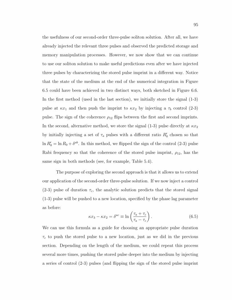
95

the usefulness of our second-order three-pulse soliton solution. After all, we have

already injected the relevant three pulses and observed the predicted storage and

memory manipulation processes. However, we now show that we can continue

to use our soliton solution to make useful predictions even after we have injected

three pulses by characterizing the stored pulse imprint in a different way. Notice

that the state of the medium at the end of the numerical integration in Figure

6.5 could have been achieved in two distinct ways, both sketched in Figure 6.6.

In the first method (used in the last section), we initially store the signal (1-3)

pulse at κx1 and then push the imprint to κx2 by injecting a τb control (2-3)

pulse. The sign of the coherence ρ12 flips between the first and second imprints.

In the second, alternative method, we store the signal (1-3) pulse directly at κx2

by initially injecting a set of τa pulses with a different ratio R′0 chosen so that

lnR′0 = lnR0 + δab. In this method, we flipped the sign of the control (2-3) pulse

Rabi frequency so that the coherence of the stored pulse imprint, ρ12, has the

same sign in both methods (see, for example, Table 5.4).

The purpose of exploring the second approach is that it allows us to extend

our application of the second-order three-pulse solution. If we now inject a control

(2-3) pulse of duration τc, the analytic solution predicts that the stored signal

(1-3) pulse will be pushed to a new location, specified by the phase lag parameter

as before:

κx3 − κx2 = δac ≡ ln

(τa + τcτa − τc

). (6.5)

We can use this formula as a guide for choosing an appropriate pulse duration

τc to push the stored pulse to a new location, just as we did in the previous

section. Depending on the length of the medium, we could repeat this process

several more times, pushing the stored pulse deeper into the medium by injecting

a series of control (2-3) pulses (and flipping the sign of the stored pulse imprint

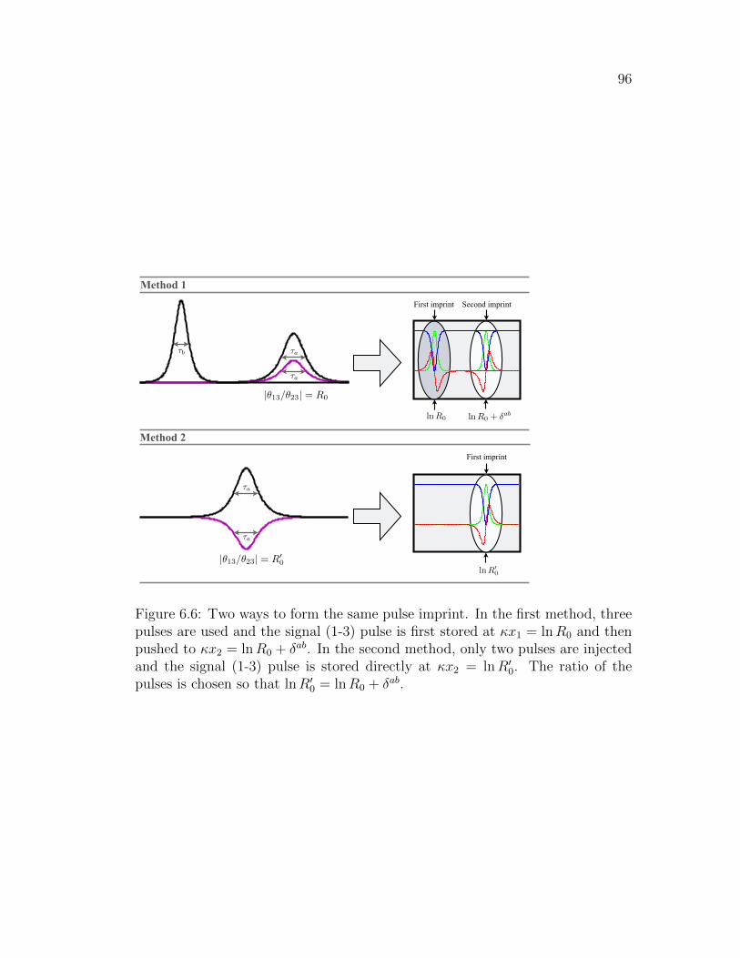
96

ln R00 (1)

13a (2)

x2 x1 = 3.560 (3)

t/a (4)

x1 = 3.000 (5)

a12 (6)

ln |R1| (7)

x1 = ln R + ab = (8)

|13/23| = R00 (9)

1/b (10)

(a12 + ab) (11)

a1 = 1, a2 = 5, a3 = i/5, (12)

a1 = 1, a2 = 5, a3 =1

5i, (13)

b1 = 0, b2 = 1, b3 = i, (14)

a = 2 b = 1, T = 25a, (15)

a1 = 1, a2 = 5, a3 =1

5i, (16)

b1 = 0, b2 = 1, b3 = i, (17)

a1 = 1 (18)

a2 = 2 (19)

aab13 (20)

↵x/2 (21)

! (22)

(23)

!3 (24)

!12 (25)

1

ln R0 + ab (1)

13a (2)

x2 x1 = 3.560 (3)

t/a (4)

x1 = 3.000 (5)

a12 (6)

ln |R1| (7)

x1 = ln R + ab = (8)

|13/23| = R00 (9)

1/b (10)

(a12 + ab) (11)

a1 = 1, a2 = 5, a3 = i/5, (12)

a1 = 1, a2 = 5, a3 =1

5i, (13)

b1 = 0, b2 = 1, b3 = i, (14)

a = 2 b = 1, T = 25a, (15)

a1 = 1, a2 = 5, a3 =1

5i, (16)

b1 = 0, b2 = 1, b3 = i, (17)

a1 = 1 (18)

a2 = 2 (19)

aab13 (20)

↵x/2 (21)

! (22)

(23)

!3 (24)

!12 (25)

1

ln R0 (1)

13a (2)

x2 x1 = 3.560 (3)

t/a (4)

x1 = 3.000 (5)

a12 (6)

ln |R1| (7)

x1 = ln R + ab = (8)

|13/23| = R0 (9)

1/b (10)

(a12 + ab) (11)

a1 = 1, a2 = 5, a3 = i/5, (12)

a1 = 1, a2 = 5, a3 =1

5i, (13)

b1 = 0, b2 = 1, b3 = i, (14)

a = 2 b = 1, T = 25a, (15)

a1 = 1, a2 = 5, a3 =1

5i, (16)

b1 = 0, b2 = 1, b3 = i, (17)

a1 = 1 (18)

a2 = 2 (19)

aab13 (20)

↵x/2 (21)

! (22)

(23)

!3 (24)

!12 (25)

1

ln R0 + ab (1)

13a (2)

x2 x1 = 3.560 (3)

t/a (4)

x1 = 3.000 (5)

a12 (6)

ln |R1| (7)

x1 = ln R + ab = (8)

|13/23| = R0 (9)

1/b (10)

(a12 + ab) (11)

a1 = 1, a2 = 5, a3 = i/5, (12)

a1 = 1, a2 = 5, a3 =1

5i, (13)

b1 = 0, b2 = 1, b3 = i, (14)

a = 2 b = 1, T = 25a, (15)

a1 = 1, a2 = 5, a3 =1

5i, (16)

b1 = 0, b2 = 1, b3 = i, (17)

a1 = 1 (18)

a2 = 2 (19)

aab13 (20)

↵x/2 (21)

! (22)

(23)

!3 (24)

!12 (25)

1

13a (1)

x2 x1 = 3.560 (2)

t/a (3)

x1 = 3.000 (4)

a12 (5)

ln |R1| (6)

x1 = ln R + ab = (7)

|13/23| = R0 (8)

1/b (9)

(a12 + ab) (10)

a1 = 1, a2 = 5, a3 = i/5, (11)

a1 = 1, a2 = 5, a3 =1

5i, (12)

b1 = 0, b2 = 1, b3 = i, (13)

a = 2 b = 1, T = 25a, (14)

a1 = 1, a2 = 5, a3 =1

5i, (15)

b1 = 0, b2 = 1, b3 = i, (16)

a1 = 1 (17)

a2 = 2 (18)

aab13 (19)

↵x/2 (20)

! (21)

(22)

!3 (23)

!12 (24)

!23 (25)

1

Method 2

b (1)

1/b (2)

a (3)

a1 = 1, a2 = 5, a3 = i/5, (4)

a1 = 1, a2 = 5, a3 =1

5i, (5)

b1 = 0, b2 = 1, b3 = i, (6)

a = 2 b = 1, T = 25a, (7)

a1 = 1, a2 = 5, a3 =1

5i, (8)

b1 = 0, b2 = 1, b3 = i, (9)

a1 = 1 (10)

a2 = 2 (11)

aab13 (12)

↵x/2 (13)

! (14)

(15)

!3 (16)

!12 (17)

!23 (18)

(19)

23 (20)

1 (21)

loc1 (22)

0.5 (23)

|131|2 (24)

1

a (1)

1/b (2)

a (3)

a1 = 1, a2 = 5, a3 = i/5, (4)

a1 = 1, a2 = 5, a3 =1

5i, (5)

b1 = 0, b2 = 1, b3 = i, (6)

a = 2 b = 1, T = 25a, (7)

a1 = 1, a2 = 5, a3 =1

5i, (8)

b1 = 0, b2 = 1, b3 = i, (9)

a1 = 1 (10)

a2 = 2 (11)

aab13 (12)

↵x/2 (13)

! (14)

(15)

!3 (16)

!12 (17)

!23 (18)

(19)

23 (20)

1 (21)

loc1 (22)

0.5 (23)

|131|2 (24)

1

a (1)

1/b (2)

a (3)

a1 = 1, a2 = 5, a3 = i/5, (4)

a1 = 1, a2 = 5, a3 =1

5i, (5)

b1 = 0, b2 = 1, b3 = i, (6)

a = 2 b = 1, T = 25a, (7)

a1 = 1, a2 = 5, a3 =1

5i, (8)

b1 = 0, b2 = 1, b3 = i, (9)

a1 = 1 (10)

a2 = 2 (11)

aab13 (12)

↵x/2 (13)

! (14)

(15)

!3 (16)

!12 (17)

!23 (18)

(19)

23 (20)

1 (21)

loc1 (22)

0.5 (23)

|131|2 (24)

1

First imprint Second imprint

a (1)

1/b (2)

a (3)

a1 = 1, a2 = 5, a3 = i/5, (4)

a1 = 1, a2 = 5, a3 =1

5i, (5)

b1 = 0, b2 = 1, b3 = i, (6)

a = 2 b = 1, T = 25a, (7)

a1 = 1, a2 = 5, a3 =1

5i, (8)

b1 = 0, b2 = 1, b3 = i, (9)

a1 = 1 (10)

a2 = 2 (11)

aab13 (12)

↵x/2 (13)

! (14)

(15)

!3 (16)

!12 (17)

!23 (18)

(19)

23 (20)

1 (21)

loc1 (22)

0.5 (23)

|131|2 (24)

1

a (1)

1/b (2)

a (3)

a1 = 1, a2 = 5, a3 = i/5, (4)

a1 = 1, a2 = 5, a3 =1

5i, (5)

b1 = 0, b2 = 1, b3 = i, (6)

a = 2 b = 1, T = 25a, (7)

a1 = 1, a2 = 5, a3 =1

5i, (8)

b1 = 0, b2 = 1, b3 = i, (9)

a1 = 1 (10)

a2 = 2 (11)

aab13 (12)

↵x/2 (13)

! (14)

(15)

!3 (16)

!12 (17)

!23 (18)

(19)

23 (20)

1 (21)

loc1 (22)

0.5 (23)

|131|2 (24)

1

First imprint

Method 1

Figure 6.6: Two ways to form the same pulse imprint. In the first method, threepulses are used and the signal (1-3) pulse is first stored at κx1 = lnR0 and thenpushed to κx2 = lnR0 + δab. In the second method, only two pulses are injectedand the signal (1-3) pulse is stored directly at κx2 = lnR′0. The ratio of thepulses is chosen so that lnR′0 = lnR0 + δab.

97

|13a|2 (1)

t/a (2)

x1 = ln R = 2.997 (3)

a12 (4)

ln |R1| (5)

x1 = ln R + ab = (6)

13/23 = |R1| (7)

1/b (8)

(a12 + ab) (9)

a1 = 1, a2 = 5, a3 = i/5, (10)

a1 = 1, a2 = 5, a3 =1

5i, (11)

b1 = 0, b2 = 1, b3 = i, (12)

a = 2 b = 1, T = 25a, (13)

a1 = 1, a2 = 5, a3 =1

5i, (14)

b1 = 0, b2 = 1, b3 = i, (15)

a1 = 1 (16)

a2 = 2 (17)

aab13 (18)

↵x/2 (19)

! (20)

(21)

!3 (22)

!12 (23)

!23 (24)

(25)

1

|13a|2 (1)

t/a (2)

x1 = ln R = 2.997 (3)

a12 (4)

ln |R1| (5)

x1 = ln R + ab = (6)

13/23 = |R1| (7)

1/b (8)

(a12 + ab) (9)

a1 = 1, a2 = 5, a3 = i/5, (10)

a1 = 1, a2 = 5, a3 =1

5i, (11)

b1 = 0, b2 = 1, b3 = i, (12)

a = 2 b = 1, T = 25a, (13)

a1 = 1, a2 = 5, a3 =1

5i, (14)

b1 = 0, b2 = 1, b3 = i, (15)

a1 = 1 (16)

a2 = 2 (17)

aab13 (18)

↵x/2 (19)

! (20)

(21)

!3 (22)

!12 (23)

!23 (24)

(25)

1

0 205 150

10

2

4

6

8

In this document, I print the equation first in black and then in white (whichof course we can’t see on the white background)

Im(13) (1)

Im(23) (2)

x (3)

23 (4)

33 (5)

(6)

@

@x+

1

c

@

@t

= iµ12 (7)

@

@x+

1

c

@

@t

= iµ12 (8)

=

Z(x, t)dt (9)

=

Z(x, t)dt (10)

vg =c

1 + (11)

vg =c

1 + (12)

xpeak = ln

inj

13

inj23

(13)

xpeak = ln

inj

13

inj23

(14)

= µ/2 (15)

1

10

2

1

4

3

Signal Pulse

In this document, I print the equation first in black and then in white (whichof course we can’t see on the white background)

Im(13) (1)

Im(23) (2)

x (3)

23 (4)

33 (5)

(6)

@

@x+

1

c

@

@t

= iµ12 (7)

@

@x+

1

c

@

@t

= iµ12 (8)

=

Z(x, t)dt (9)

=

Z(x, t)dt (10)

vg =c

1 + (11)

vg =c

1 + (12)

xpeak = ln

inj

13

inj23

(13)

xpeak = ln

inj

13

inj23

(14)

= µ/2 (15)

1

108642

In this document, I print the equation first in black and then in white (whichof course we can’t see on the white background)

(1)

Im(13) (2)

Im(23) (3)

x (4)

t

s(5)

t/s (6)

23 (7)

33 (8)

(9)

@

@x+

1

c

@

@t

= iµ12 (10)

@

@x+

1

c

@

@t

= iµ12 (11)

=

Z(x, t)dt (12)

=

Z(x, t)dt (13)

vg =c

1 + (14)

vg =c

1 + (15)

xpeak = ln

inj

13

inj23

(16)

xpeak = ln

inj

13

inj23

(17)

1

0

Pulse Areas

In this document, I print the equation first in black and then in white (whichof course we can’t see on the white background)

loc1 (1)

1.5 (2)

|13s|2 (3)

Im(13) (4)

Im(23) (5)

x (6)

t

s(7)

t/s (8)

23 (9)

33 (10)

(11)

@

@x+

1

c

@

@t

= iµ12 (12)

@

@x+

1

c

@

@t

= iµ12 (13)

=

Z(x, t)dt (14)

=

Z(x, t)dt (15)

vg =c

1 + (16)

vg =c

1 + (17)

xpeak = ln

inj

13

inj23

(18)

1

In this document, I print the equation first in black and then in white (whichof course we can’t see on the white background)

loc1 (1)

2 (2)

|13s|2 (3)

Im(13) (4)

Im(23) (5)

x (6)

t

s(7)

t/s (8)

23 (9)

33 (10)

(11)

@

@x+

1

c

@

@t

= iµ12 (12)

@

@x+

1

c

@

@t

= iµ12 (13)

=

Z(x, t)dt (14)

=

Z(x, t)dt (15)

vg =c

1 + (16)

vg =c

1 + (17)

xpeak = ln

inj

13

inj23

(18)

1

In this document, I print the equation first in black and then in white (whichof course we can’t see on the white background)

loc1 (1)

0.5 (2)

|13s|2 (3)

Im(13) (4)

Im(23) (5)

x (6)

t

s(7)

t/s (8)

23 (9)

33 (10)

(11)

@

@x+

1

c

@

@t

= iµ12 (12)

@

@x+

1

c

@

@t

= iµ12 (13)

=

Z(x, t)dt (14)

=

Z(x, t)dt (15)

vg =c

1 + (16)

vg =c

1 + (17)

xpeak = ln

inj

13

inj23

(18)

1

In this document, I print the equation first in black and then in white (whichof course we can’t see on the white background)

23 (1)

x1 (2)

x2 (3)

1 (4)

loc1 (5)

0.5 (6)

|131|2 (7)

Im(13) (8)

Im(23) (9)

x (10)

t

1(11)

t/1 (12)

23 (13)

33 (14)

(15)

@

@x+

1

c

@

@t

= iµ12 (16)

@

@x+

1

c

@

@t

= iµ12 (17)

=

Z(x, t)dt (18)

=

Z(x, t)dt (19)

vg =c

1 + (20)

1

Figure 6.7: Results of a numerical integration after the τc control (2-3) pulseenters the medium. The recovered signal (1-3) pulse is shown and the areas ofboth pulses are plotted in the inset.

each time).

For illustration, we now show how to retrieve the signal (1-3) pulse we

stored at κx2 = 6.56 in the previous section. Our aim is to choose a new storage

location that is well outside the boundary of the medium (at κx = 10) so that

essentially no information (excitation) is left behind. Using equation 6.5 as our

guide, we chose τc = 0.999τa so that κx3 = 14.16. As before, we injected a

strong, 2π-area control (2-3) pulse in the imprinted medium. The results of the

numerical simulation are shown in Figure 6.7. The figure shows that at the edge

of the medium (at κx = 10), the recovered signal (1-3) pulse is nearly identical

to its original form (compare with the pulse at κx = 0 in Figure 6.3). We can

calculate the fidelity of the entire multi-step process, defined by the ratio of the

98

output and input intensities of the signal (1-3) pulse:

F =

∫|Ωout

13 (x, t)|2dt∫|Ωin

13(x, t)|2dt × 100%. (6.6)

For the numerical integration shown, we find a remarkably high fidelity of 99%.

6.2.3 Non-Idealized Input Pulse Conditions

Using our second-order three-pulse soliton solution to obtain control pa-

rameters, we have demonstrated precise storage, manipulation, and high-fidelity

retrieval of broadband information in a finite medium. The numerical integration

we analyzed in the previous sections were for pulses with finite tails but perfect,

idealized, 2π-area hyperbolic secant shapes. With less idealized input pulses, we

find that the basic control procedures we have outlined remain relevant and our

soliton solution continues to offer useful predictions. When the injected pulse

areas differ significantly from the analytically stable 2π values, pulse ringing can

become noticeable, in the same way it was for two-level media.

To help quantity the effects of deviations, we show a specific example in

Figure 6.8. There, we plot the final (recovered) signal (1-3) pulse and the state of

the medium (now located between κx = 0 and κx = 15). In this simulation, we

injected Gaussian pulses with an area of 1.9π (rather than 2π) but used the same

relationships between the pulse widths as before (τb = 0.95τa and τc = 0.999τa).

We find that the area of the retrieved signal (1-3) pulse grows to 1.97π in the

process and the initially Gaussian pulse is reshaped into a hyperbolic secant.

The amount of ringing on the signal (1-3) pulse is just barely visible and the

total fidelity remains high at 96.7%. As deviations from the idealized input

conditions increase, so does the amplitude of the pulse ringing. Our numerical

solutions indicate that the high bandwidth optical pulse control techniques we

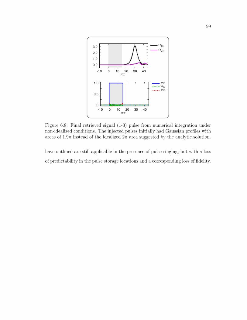
99

0.0

1.0

2.0

3.0

-10 0 10 20 30 40

0

0.5

1.0

-10 0 10 20 30 40

-0.5

0

0.5

1.0

-10 0 10 20 30 40

In this document, I print the equation first in black and then in white (whichof course we can’t see on the white background)

Im(13) (1)

Im(23) (2)

x (3)

23 (4)

33 (5)

(6)

@

@x+

1

c

@

@t

= iµ12 (7)

@

@x+

1

c

@

@t

= iµ12 (8)

=

Z(x, t)dt (9)

=

Z(x, t)dt (10)

vg =c

1 + (11)

vg =c

1 + (12)

xpeak = ln

inj

13

inj23

(13)

xpeak = ln

inj

13

inj23

(14)

= µ/2 (15)

1

In this document, I print the equation first in black and then in white (whichof course we can’t see on the white background)

Im(13) (1)

Im(23) (2)

x (3)

23 (4)

33 (5)

(6)

@

@x+

1

c

@

@t

= iµ12 (7)

@

@x+

1

c

@

@t

= iµ12 (8)

=

Z(x, t)dt (9)

=

Z(x, t)dt (10)

vg =c

1 + (11)

vg =c

1 + (12)

xpeak = ln

inj

13

inj23

(13)

xpeak = ln

inj

13

inj23

(14)

= µ/2 (15)

1

0.0

1.0

2.0

-10 0 10 20 30 40

0

0.5

1.0

-10 0 10 20 30 40

-0.5

0

0.5

1.0

-10 0 10 20 30 40

-1.6

-0.8

0

0.8

1.6

-10 -5 0 5 10 15 20

-0.5

0

0.5

1.0

-10 -5 0 5 10 15 20

x (34)

=

11 12

21 22

(35)

=

11 12

21 22

(36)

H = h

2

0@

0 0 13

0 0 23

13 23 0

1A (37)

H = h

2

0@

0 0 13

0 0 23

13 23 0

1A (38)

H = h

2

0

13

13 0

(39)

H = h

2

0

0

(40)

H = h

2

0

0

(41)

ih@

@t= [H, ] (42)

ih@

@t= [H, ] (43)

@

@x+

1

c

@

@t

13 = iµ1313 (44)

@

@x+

1

c

@

@t

13 = iµ2323 (45)

@

@x+

1

c

@

@t

23 = iµ1313 (46)

@

@x+

1

c

@

@t

23 = iµ2323 (47)

3

In this document, I print the equation first in black and then in white (whichof course we can’t see on the white background)

23 (1)

1 (2)

loc1 (3)

0.5 (4)

|131|2 (5)

Im(13) (6)

Im(23) (7)

x (8)

t

1(9)

t/1 (10)

23 (11)

33 (12)

(13)

@

@x+

1

c

@

@t

= iµ12 (14)

@

@x+

1

c

@

@t

= iµ12 (15)

=

Z(x, t)dt (16)

=

Z(x, t)dt (17)

vg =c

1 + (18)

vg =c

1 + (19)

1

-1.6

-0.8

0

0.8

1.6

-10 -5 0 5 10 15 20

-0.5

0

0.5

1.0

-10 -5 0 5 10 15 20

xpeak = lninj

13 /inj23

(14)

xpeak = lninj

13 /inj23

(15)

= 0.9 storage (16)

storage (17)

storage (18)

control (19)

control (20)

xmove = ln

storage control

storage + control

(21)

xmove = ln

storage control

storage + control

(22)

x (23)

=

11 12

21 22

(24)

=

11 12

21 22

(25)

H = h

2

0@

0 0 13

0 0 23

13 23 0

1A (26)

H = h

2

0@

0 0 13

0 0 23

13 23 0

1A (27)

H = h

2

0

13

13 0

(28)

2

xpeak = lninj

13 /inj23

(14)

xpeak = lninj

13 /inj23

(15)

= 0.9 storage (16)

storage (17)

storage (18)

control (19)

control (20)

xmove = ln

storage control

storage + control

(21)

xmove = ln

storage control

storage + control

(22)

x (23)

=

11 12

21 22

(24)

=

11 12

21 22

(25)

H = h

2

0@

0 0 13

0 0 23

13 23 0

1A (26)

H = h

2

0@

0 0 13

0 0 23

13 23 0

1A (27)

H = h

2

0

13

13 0

(28)

2

= µs/2 (14)

xpeak = lninj

13 /inj23

(15)

xpeak = lninj

13 /inj23

(16)

= 0.9 storage (17)

storage (18)

storage (19)

control (20)

control (21)

xmove = ln

storage control

storage + control

(22)

xmove = ln

storage control

storage + control

(23)

x (24)

=

11 12

21 22

(25)

=

11 12

21 22

(26)

H = h

2

0@

0 0 13

0 0 23

13 23 0

1A (27)

H = h

2

0@

0 0 13

0 0 23

13 23 0

1A (28)

2

-1.6

-0.8

0

0.8

1.6

-10 -5 0 5 10 15 20

-0.5

0

0.5

1.0

-10 -5 0 5 10 15 20

Figure 6.8: Final retrieved signal (1-3) pulse from numerical integration undernon-idealized conditions. The injected pulses initially had Gaussian profiles withareas of 1.9π instead of the idealized 2π area suggested by the analytic solution.

have outlined are still applicable in the presence of pulse ringing, but with a loss

of predictability in the pulse storage locations and a corresponding loss of fidelity.

100

Chapter 7

Conclusions

We have pursued a theoretical model for short optical pulses propagating

in resonant, absorbing media. Previous work has shown that such media can

be used to slow, stop, and store optical pulses, enhancing possibilities for opti-

cal communication networks in this domain. However, most techniques impose

bandwidth limitations on the signal pulse and cannot be applied to the short,

broadband pulses we study. We have proposed a new method of optical pulse

storage, capable of converting and recovering a high-bandwidth signal pulse with

high fidelity. We derived a novel soliton solution to find the necessary control

parameters and applied an innovative extrapolation of our solution to numerical

solutions in finite-length media to achieve predictive optical information storage

and transfer. We summarize our central findings and suggest potential future

directions of our research below.

We derived the nonlinear partial differential equations characterizing short-

pulse propagation in resonant media in Chapter 2. There, we highlighted known

features in this regime, including the phenomenon of Self-Induced Transparency

(SIT) and the pulse Area Theorem. We also derived the relevant nonlinear evolu-

tion equations for two-pulse propagation in three-level Λ-type media. We devel-

oped the mathematical framework necessary to derive new, exact soliton solutions

to these equations in Chapter 3. We used the matrix Darboux transformation

method and derived a related nonlinear superposition rule to enable production

101

of new soliton solutions with algebraic techniques. Informally, we defined soli-

tons as exact analytic solutions that can be nonlinearly superimposed (collided)

to form more complicated solutions.

We illustrated our solution method first in Chapter 4 by deriving previ-

ously known soliton solutions for coherent pulse propagation in two-level media.

We showed that the 2π-area hyperbolic secant pulse associated with Self-Induced

Transparency (SIT) [39] is an exact, first-order soliton solution. We superim-

posed two of these SIT-type solutions to create a second-order soliton solution

and illustrate a hallmark property of soliton solutions: that they collide elastically

like particles by separating into two co-propagating first-order solitons before and

after the collision.

To find a model for high-bandwidth optical pulse control, we derived three

exact soliton solutions for Λ-type media in Chapter 5. The first was a first-order

two-pulse soliton solution, previously characterized by Clader and Eberly [45]

that describes the conversion of a strong signal pulse into a redistribution of

population of the long-lived ground-state density matrix elements of the atoms

(forming an imprint, or memory of the signal pulse). The second (also first-

order) soliton solution was a new solution that we designed to model the retrieval

process. We nonlinearly superimposed these two solutions to produce our novel

third (three-pulse second-order) soliton solution. After carefully examining the

behavior of this solution in the limits of large positive and negative time, we

made appropriate choices of the integration constants to find a solution modeling

optical pulse storage and memory manipulation. An important result was that

we discovered that we could push the stored pulse imprint to a new, predictable

location by controlling the signal and control pulse durations.

Soliton solutions are desirable because they have such clearly defined con-

102

trol parameters, but also because they are generally robust and stable under

non-idealized conditions. In Chapter 6, we tested the stability of our soliton so-

lutions by numerically integrating the nonlinear evolution equations for two-level

and three-level systems in finite media. We used an implicit-trapezoidal method

and chose input parameters based on our analytic solutions. With our second-

order soliton solution for three-level media as a model, we stored a realistic (with

finite tails) hyperbolic secant signal pulse in an absorbing three-level medium

and predicted the storage location with less than 1% deviation from the analytic

solution. We then injected a control pulse to push the imprint to a new location,

carefully tuning the control pulse duration so that minimal signal pulse infor-

mation was ejected from the medium before desirable. Comparing our results

with our soliton solution, we accurately predicted the second storage location to

within 2% error. Finally, we injected a new control pulse to recover the stored

signal pulse and restore the medium to its initial configuration. By modeling the

entire multistep procedure with our three-pulse second-order soliton solution, we

recovered the signal pulse with an exceptionally high fidelity of 99%.

7.1 Future Directions

The control parameters suggested by our second-order soliton solution

make it a reliable model for optical pulse storage and retrieval for short, high-

bandwidth pulses. There are, however, several factors that naturally degrade

the fidelity of the process. Deviations from the optimized 2π-area hyperbolic se-

cant input pulses cause transient pulse ringing and small-amplitude fluctuations

between the atomic ground and excited state populations. Our numerical ex-

periments indicate that these fluctuations have little effect on the fidelity of the

recovered signal pulse even for area deviations as large as 25%. However, larger

103

deviations from the optimal 2π area take one out of the zone of applicability of

our solution. Pulses that are too weak (areas near or below 1π) cannot promote

a sufficient proportion of the atoms to the excited state and are quickly depleted.

Promoting the atoms to the excited state is an essential step in the imprinting

process and, without it, the signal pulse is not converted and its information is

lost.

Pulses that are significantly stronger (areas greater than 3π) induce the

necessary excitation, but we find that these pulses break up just as they do

in two-level media. These large-area pulses quickly become well-separated 2π-

area pulses that are stored at different locations throughout the medium. The

behavior of these large-area pulses can be explained from soliton theory. For

example, in two-level media the pulse break-up reported by McCall and Hahn

[38] can be explained as the “second-half” of a collision in a 4π-area soliton

solution. Similarly, in three-level media, higher-order soliton solutions exist with

total areas of 6π, 8π, and so on and by injecting large-area pulses, we essentially

simulate those solutions. A natural extension of our research would be to derive

and analyze these higher-order solutions to examine possibilities for multi-pulse

storage and manipulation.

Our current proposal applies to pulses short enough that we can justifiably

neglect all atomic decay channels, as appropriate for ultra-cold atoms. Ultra-cold

atoms are excellent candidates for optical pulse control because of their long-

lived ground states; however, preparing the atomic medium can be difficult and

requires specialized techniques. To successfully model room-temperature or hot

atomic vapors, one would need to extend our research to include sources of inho-

mogeneous relaxation, such as Doppler broadening. In that case, the absorption

coefficient would be defined differently [45] but the basic storage procedure would

104

carry through with the added stability expected from Self-Induced Transparency

effects. This would be an interesting avenue to pursue in order to effectively

model high-bandwidth pulse storage in room temperature vapors.

The short pulses we model escape the effects of homogeneous broadening

from, for example, spontaneous emission. However, once imprinted, the stored

pulse information is encoded on the ground-state density matrix elements of the

atoms. The lifetime of the imprint, then, is limited by the homogeneous lifetime

of those states. Typically, the atomic coherence is the limiting factor because

it is lost at a faster rate compared with the atomic populations due to soft,

inter-atom collisions. It would be interesting to explore the effect of this finite

coherence lifetime on the storage and retrieval process with numerical solutions.

It is conceivable that one may be able to extend the storage time by pushing

the tightly compressed imprint back and forth between discrete locations using a

series of control pulses.

In sum, we combined computational and analytical techniques to model

short optical pulse control in resonant media. The relevant nonlinear evolution

equations support soliton pulse propagation and we derived soliton solutions that

are robust and predictable even in finite media with non-idealized input pulses.

Using our novel three-pulse second-order soliton solution, we developed a scheme

to store broadband pulse information in an absorbing medium and manipulate its

location with minimal degradation of the signal pulse. Adapting our solutions to

finite-length media, we showed how to retrieve the stored information on-demand

with little distortion of the signal pulse and remarkably high fidelity.

BIBLIOGRAPHY 105

Bibliography

[1] S. E. Harris, “Electromagnetically induced transparency,” Phys. Today 50,

36 (1997), URL http://dx.doi.org/10.1063/1.881806.

[2] M. Fleischhauer, A. Imamoglu, and J. P. Marangos, “Electromagnetically

induced transparency: Optics in coherent media,” Rev. Mod. Phys. 77, 633

(2005), URL http://link.aps.org/doi/10.1103/RevModPhys.77.633.

[3] P. W. Milonni, Fast Light, Slow Light, and Left-Handed Light (Taylor and

Francis Group, New York, 2005).

[4] C. Liu and Z. Dutton, “Observation of coherent optical information storage

in an atomic medium using halted light pulses,” Nature 409, 490 (2000),

URL http://dx.doi.org/10.1038/35054017.

[5] N. S. Ginsberg, S. R. Garner, and L. V. Hau, “Coherent control of optical

information with matter wave dynamics,” Nature 445, 623 (2007), URL

http://dx.doi.org/10.1038/nature05493.

[6] D. F. Phillips, A. Fleischhauer, A. Mair, R. L. Walsworth, and M. D. Lukin,

“Storage of light in atomic vapor,” Phys. Rev. Lett. 86, 783 (2001), URL

http://link.aps.org/doi/10.1103/PhysRevLett.86.783.

[7] I. Novikova, A. V. Gorshkov, D. F. Phillips, A. S. Sørensen, M. D. Lukin,

and R. L. Walsworth, “Optimal control of light pulse storage and retrieval,”

Phys. Rev. Lett. 98, 243602 (2007), URL http://link.aps.org/doi/10.

1103/PhysRevLett.98.243602.

[8] G.-J. Yang, T. Qiu, K. Wang, and M. Xie, “Reversible storage of a weak

light pulse in a thermal atomic medium,” Phys. Rev. A 81, 063817 (2010),

URL http://link.aps.org/doi/10.1103/PhysRevA.81.063817.

[9] J. J. Longdell, E. Fraval, M. J. Sellars, and N. B. Manson, “Stopped light

with storage times greater than one second using electromagnetically induced

transparency in a solid,” Phys. Rev. Lett. 95, 063601 (2005), URL http:

//link.aps.org/doi/10.1103/PhysRevLett.95.063601.

[10] M. Afzelius, C. Simon, H. de Riedmatten, and N. Gisin, “Multimode quan-

tum memory based on atomic frequency combs,” Phys. Rev. A 79, 052329

(2009), URL http://link.aps.org/doi/10.1103/PhysRevA.79.052329.

BIBLIOGRAPHY 106

[11] S. A. Moiseev and S. Kroll, “Complete reconstruction of the quantum state

of a single-photon wave packet absorbed by a doppler-broadened transition,”

Phys. Rev. Lett. 87, 173601 (2001), URL http://link.aps.org/doi/10.

1103/PhysRevLett.87.173601.

[12] G. Hetet, J. J. Longdell, A. L. Alexander, P. K. Lam, and M. J. Sell-

ars, “Electro-optic quantum memory for light using two-level atoms,” Phys.

Rev. Lett. 100, 023601 (2008), URL http://link.aps.org/doi/10.1103/

PhysRevLett.100.023601.

[13] M. P. Hedges, J. J. Longdell, Y. Li, and M. J. Sellars, “Efficient quantum

memory for light,” Nature 465, 1052 (2010), URL http://dx.doi.org/10.

1038/nature09081.

[14] H. de Riedmatten, M. Afzelius, M. U. Staudt, C. Simon, and N. Gisin, “A

solid-state light-matter interface at the single-photon level,” Nature 456,

773 (2008), URL http://dx.doi.org/10.1038/nature07607.

[15] K. F. Reim, J. Nunn, V. O. Lorenz, B. J. Sussman, K. C. Lee, L. N. K., J. D.,

and W. I. A., “Towards high-speed optical quantum memories,” Nat. Pho-

tonics 4, 218 (2010), URL http://dx.doi.org/10.1038/nphoton.2010.

30.

[16] J.-L. Le Gouet and P. R. Berman, “Raman scheme for adjustable-bandwidth

quantum memory,” Phys. Rev. A 80, 012320 (2009), URL http://link.

aps.org/doi/10.1103/PhysRevA.80.012320.

[17] J. Nunn, I. A. Walmsley, M. G. Raymer, K. Surmacz, F. C. Waldermann,

Z. Wang, and D. Jaksch, “Mapping broadband single-photon wave packets

into an atomic memory,” Phys. Rev. A 75, 011401 (2007), URL http://

link.aps.org/doi/10.1103/PhysRevA.75.011401.

[18] T. Golubeva, Y. Golubev, O. Mishina, A. Bramati, J. Laurat, and E. Gi-

acobino, “High-speed spatially multimode atomic memory,” Phys. Rev. A

83, 053810 (2011), URL http://link.aps.org/doi/10.1103/PhysRevA.

83.053810.

[19] A. V. Backlund, “Om ytor med konstant negativ krokning,” Lunds Univer-

sitets 19, 1 (1883).

[20] G. Darboux, “Sur une proposition relative aux equations linearies,” C. R.

Acad. Sci. Paris 94, 1456 (1882).

BIBLIOGRAPHY 107

[21] M. M. Crum, “Associated Sturm-Liouville systems,” Q. J. Math Oxford 6,

121 (1955).

[22] M. Wadati, H. Sanuki, and K. Kimaiki, “Relationships among inverse

method, backlund transformation and an infinite number of conservation

laws,” Prog. Theor. Phys. 53, 419 (1975), URL http://ptp.ipap.jp/link?

PTP/53/419/.

[23] C. Rogers and W. K. Schief, Backlund and Darboux Transformations: Ge-

ometry and Modern Applications in Soliton Theory (Cambridge University

Press, Cambridge, 2002).

[24] C. S. Gardner, J. M. Greene, M. D. Kruskal, and R. M. Miura, “Method for

solving the Korteweg-de Vries equation,” Phys. Rev. Lett. 19, 1095 (1967),

URL http://link.aps.org/doi/10.1103/PhysRevLett.19.1095.

[25] V. E. Zakharov and A. B. Shabat, “Exact theory of two-dimensional self-

focusing and one-dimensional self-modulation of waves in nonlinear media,”

Sov. Phys. JETP 34, 62 (1972).

[26] M. J. Ablowitz, D. J. Kaup, A. C. Newell, and H. Segur, “Nonlinear-

evolution equations of physical significance,” Phys. Rev. Lett. 31, 125 (1973),

URL http://link.aps.org/doi/10.1103/PhysRevLett.31.125.

[27] P. D. Lax, “Integrals of nonlinear equations of evolution and solitary waves,”

Comm. Pure Appl. Math. 21, 467 (1968), URL http://dx.doi.org/10.

1002/cpa.3160210503.

[28] C. Gu, H. Hu, and Z. Zhou, Darboux Transformations in Integrable Systems

(Springer, Dordrecht, 2005).

[29] V. B. Matveev and M. A. Salle, Darboux Transformations and Solitons

(Springer-Verlag, Berlin, 1991).

[30] G. Neugebauer and R. Meinel, “General N-soliton solution of the AKNS

class on arbitrary background,” Physics Letters A 100, 467 (1984), ISSN

0375-9601, URL http://www.sciencedirect.com/science/article/pii/

0375960184908272.

[31] J. L. Cieslinski, “An algebraic method to construct the Darboux matrix,”

Journal of Mathematical Physics 36, 5670 (1995), URL http://link.aip.

org/link/?JMP/36/5670/1.

BIBLIOGRAPHY 108

[32] J. L. Cieslinski, “Algebraic representation of the linear problem as a method

to construct the Darboux-Backlund transformation,” Chaos, Solitons, Frac-

tals 5, 2303 (1995), URL http://dx.doi.org/10.1016/0960-0779(94)

E0100-4.

[33] J. L. Cieslinski, “Algebraic construction of the Darboux matrix revisited,”

Journal of Physics A: Mathematical and Theoretical 42, 404003 (2009), ISSN

1751-8113, URL http://stacks.iop.org/1751-8121/42/i=40/a=404003?

key=crossref.0b9e9dc8cecd8ccab17c445b63fc3651.

[34] N. J. Zabusky and M. D. Kruskal, “Interaction of ‘solitons’ in a collisionless

plasma and the recurrence of initial states,” Phys. Rev. Lett. 15, 240 (1965),

URL http://link.aps.org/doi/10.1103/PhysRevLett.15.240.

[35] M. J. Ablowitz, G. Biondini, and L. A. Ostrovsky, “Optical solitons: Per-

spectives and applications,” Chaos 10, 471 (2000), URL http://dx.doi.

org/10.1063/1.1310721.

[36] L. Allen and J. H. Eberly, Optical Resonance and Two-Level Atoms (Wiley,

New York, 1975).

[37] G. L. Lamb Jr., Elements of Soliton Theory (Wiley, New York, 1980).

[38] S. L. McCall and E. L. Hahn, “Self-induced transparency,” Phys. Rev. 183,

457 (1969), URL http://link.aps.org/doi/10.1103/PhysRev.183.457.

[39] S. L. McCall and E. L. Hahn, “Self-induced transparency by pulsed coherent

light,” Phys. Rev. Lett. 18, 908 (1967).

[40] D. A. Steck, “Rubidium 87 D line data,” (2001), URL http://steck.us/

alkalidata/.

[41] G. L. Lamb Jr., “Propagation of ultrashort optical pulses,”

Physics Letters A 25, 181 (1967), ISSN 0375-9601, URL http:

//www.sciencedirect.com/science/article/B6TVM-46T4K00-C3/2/

9b06e0d81ca4e2e08847dc2e6c65aa0c.

[42] Q.-H. Park and H. Shin, “Classical matrix Sine-Gordon theory,” Nu-

clear Physics B 458, 327 (1996), ISSN 0550-3213, URL http://www.

sciencedirect.com/science/article/pii/0550321395005390.

[43] Q.-H. Park and H. J. Shin, “Field theory for coherent optical pulse propa-

gation,” Phys. Rev. A 57, 4621 (1998).

BIBLIOGRAPHY 109

[44] Q.-H. Park and H. Shin, “Matched pulse propagation in a three-level sys-

tem,” Physical Review A 57, 4643 (1998), ISSN 1050-2947, URL http:

//link.aps.org/doi/10.1103/PhysRevA.57.4643.

[45] B. Clader and J. Eberly, “Two-pulse propagation in media with quantum-

mixed ground states,” Physical Review A 76, 053812 (2007), ISSN 1050-

2947, URL http://link.aps.org/doi/10.1103/PhysRevA.76.053812.

[46] R. Hirota, The Direct Method in Soliton Theory (Cambridge University

Press, 2004).

[47] L. R. T. Gardner, G. A. Gardner, and T. Geyikli, “Solitary wave

solutions of the MKdV equation,” Computer Methods in Applied

Mechanics and Engineering 124, 321 (1995), ISSN 0045-7825, URL

http://www.sciencedirect.com/science/article/B6V29-3XX6V0J-R/

2/9b3731f3b27478c4fc7218069a2b4cba.

[48] A. Scott, F. Chu, and D. McLaughlin, “The soliton: A new concept in

applied science,” Proceedings of the IEEE 61, 1443 (1973), ISSN 0018-

9219.

[49] E. Groves, B. D. Clader, and J. H. Eberly, “Multipulse quantum con-

trol: exact solutions,” Opt. Lett. 34, 2539 (2009), URL http://www.

opticsinfobase.org/ol/abstract.cfm?uri=ol-34-16-2539.

[50] B. D. Clader and J. H. Eberly, “Two-pulse propagation in a partially phase-

coherent medium,” Phys. Rev. A 78, 033803 (2008), URL http://link.

aps.org/doi/10.1103/PhysRevA.78.033803.

[51] W. H. Press, S. A. Teulosky, W. T. Vetterling, and B. P. Flannery, Numer-

ical Recipes: The Art of Scientific Computing, Third Edition (Cambridge

University Press, Cambridge, 2007).

[52] B. D. Clader, “Ultra-short pulse propagation in multi-level media,” Ph.D.

thesis, University of Rochester (2008), URL http://hdl.handle.net/

1802/6273.

[53] G. L. Lamb Jr., “Analytical descriptions of ultrashort optical pulse prop-

agation in a resonant medium,” Rev. Mod. Phys. 43, 99 (1971), URL

http://link.aps.org/doi/10.1103/RevModPhys.43.99.