Solid-State Kinetic Models

Subscriber access provided by MERCER UNIV

The Journal of Physical Chemistry B is published by the American Chemical Society.1155 Sixteenth Street N.W., Washington, DC 20036

Review Articles

Solid-State Kinetic Models: Basics and Mathematical FundamentalsAmmar Khawam, and Douglas R. Flanagan

J. Phys. Chem. B, 2006, 110 (35), 17315-17328 • DOI: 10.1021/jp062746a

Downloaded from http://pubs.acs.org on December 4, 2008

More About This Article

Additional resources and features associated with this article are available within the HTML version:

• Supporting Information• Links to the 6 articles that cite this article, as of the time of this article download• Access to high resolution figures• Links to articles and content related to this article• Copyright permission to reproduce figures and/or text from this article

http://pubs.acs.org/doi/full/10.1021/jp062746a

REVIEW ARTICLES

Solid-State Kinetic Models: Basics and Mathematical Fundamentals

Ammar Khawam and Douglas R. Flanagan*DiVision of Pharmaceutics, College of Pharmacy, UniVersity of Iowa, Iowa City, Iowa 52242

ReceiVed: May 5, 2006; In Final Form: June 25, 2006

Many solid-state kinetic models have been developed in the past century. Some models were based onmechanistic grounds while others lacked theoretical justification and some were theoretically incorrect. Modelscurrently used in solid-state kinetic studies are classified according to their mechanistic basis as nucleation,geometrical contraction, diffusion, and reaction order. This work summarizes commonly employed modelsand presents their mathematical development.

1. Introduction

Fifty years have passed since the publication ofChemistryof the Solid State, edited by W. E. Garner,1 which coveredtheories of the solid state, including solid-state reaction kinetics.Jacobs and Tompkins2 covered theories and derivations of somesolid-state reaction models in Garner’s text, specifically,nucleation and nuclei growth models. The derivation of theseand other models has also appeared in Volume 22 of theChemical Kinetics Seriesentitled, “Reactions in the Solid State”by Brown et al.3 Later, Galwey and Brown4 presented many ofthese same models. These and other older references arebecoming less accessible because they have been out of printfor many years. Researchers who seek the basis for these modelsand their mathematical foundations must find such old texts oraccess even older journal articles. Unfortunately, no singlereference comprehensively presents the basics and mathematicaldevelopment of these models. The lack of such a source causesauthors to redundantly present reaction models in tabularform5-10 as shown in Table 1. It is rare to find a solid-statekinetic report that does not list such reaction models becauseof the lack of a general source to which reference can be made.

This review is intended to provide a summary and math-ematical basis for commonly used reaction models in solid-state kinetics.

2. Reaction Rate Laws

The rate of a solid-state reaction can be generally describedby

where, A is the preexponential (frequency) factor,Ea is theactivation energy,T is absolute temperature,R is the gasconstant,f(R) is the reaction model, andR is the conversion

fraction. For a gravimetric measurement,R is defined by

where,m0 is initial weight, mt is weight at timet, andm∞ isfinal weight.

Kinetic parameters (model,A, Ea) can be obtained fromisothermal kinetic data by applying the above rate law (eq 1).Alternatively, eq 1 can be transformed into a nonisothermal rateexpression describing reaction rate as a function of temperatureat a constant heating rate by utilizing the following:

where, dR/dT is the nonisothermal reaction rate, dR/dt is theisothermal reaction rate, and dT/dt is the heating rate (â).Substituting eq 1 into eq 3 gives the differential form of thenonisothermal rate law,

Separating variables and integrating eqs 1 and 4 gives theintegral forms of the isothermal and nonisothermal rate laws,respectively:

and

where,g(R) is the integral reaction model, defined by

It should be noted that there is no consensus on the symbolsused to represent these models, so the definitions off(R) and

* Corresponding author: E-mail address: [email protected]: (319) 335-9349.

dRdt

) Ae-(Ea/RT) f(R) (1)

R )m0 - mt

m0 - m∞(2)

dRdT

) dRdt

dtdT

(3)

dRdT

) Aâ

e-(Ea/RT) f(R) (4)

g(R) ) Ae-(Ea/RT) t (5)

g(R) ) Aâ∫0

Te-(Ea/RT) dT (6)

g(R) ) ∫0

R dRf(R)

17315J. Phys. Chem. B2006,110,17315-17328

10.1021/jp062746a CCC: $33.50 © 2006 American Chemical SocietyPublished on Web 08/15/2006

g(R) may be reversed in some publications. Several reactionmodels (f(R) andg(R)) are listed in Table 1.

Reaction kinetics in the solid-state are often studied bythermogravimetry, but they can also be studied by otheranalytical methods such as differential scanning calorimetry(DSC),11,12 powder X-ray diffraction (PXRD),13 and nuclearmagnetic resonance (NMR).14,15For any analytical method, themeasured parameter must be able to be transformed into aconversion fraction (R) that can be used in the kinetic equations.

Kinetic analysis (isothermal or nonisothermal) can be per-formed by either model-fitting or model-free (isoconversional)methods.11 The use of isoconversional or model-free methodshas increased recently12,16-21 due to the ability of these methodsto calculateEa values without modelistic assumptions. However,such methods have some disadvantages,22,23 and a reactionmodel is usually needed for a complete kinetic description ofany solid-state reaction.24 Different solid-state kinetic analysismethods have been recently reviewed.11

3. Models and Mechanisms in Solid-State Kinetics

A model is a theoretical, mathematical description of whatoccurs experimentally. In solid-state reactions, a model candescribe a particular reaction type and translate that mathemati-cally into a rate equation. Many models have been proposed insolid-state kinetics, and these models have been developed basedon certain mechanistic assumptions. Other models are moreempirically based, and their mathematics facilitates data analysiswith little mechanistic meaning. Therefore, different rate expres-sions are produced from these models.

In homogeneous kinetics (e.g., gas or solution phases), kineticstudies are usually directed toward obtaining rate constants thatcan be used to describe the progress of a reaction. Additionally,the reaction mechanism is typically investigated and rateconstant changes with temperature, pressure, or reactant/productconcentrations are often helpful in uncovering mechanisms.These mechanisms involve to varying degrees the detailed

Ammar M. N. Khawam received his B.S. in Pharmacy from the JordanUniversity of Science and Technology in 1997. After working in thepharmaceutical industry, he joined the graduate program at theUniversity of Iowa and is completing his Ph.D. degree in Pharmaceutics.His research interests include physical properties of solids, drug stability,and thermal analysis applications to pharmaceutical development.

TABLE 1: Solid-State Rate and Integral Expressions for Different Reaction Models

modeldifferential formf(R) ) 1/k dR/dt

integral formg(R) ) kt

nucleation modelspower law (P2) 2R1/2 R1/2

power law (P3) 3R2/3 R1/3

power law (P4) 4R3/4 R1/4

Avrami-Erofeyev (A2) 2(1- R)[-ln(1 - R)]1/2 [-ln(1 - R)]1/2



Prout-Tompkins (B1) R(1 - R) ln[R/(1 - R)] + ca

geometrical contraction modelscontracting area (R2) 2(1- R)1/2 1 - (1 - R)1/2

contracting volume (R3) 3(1- R)2/3 1 - (1 - R)1/3

diffusion models1-D diffusion (D1) 1/(2R) R2

2-D diffusion (D2) -[1/ln(1 - R)] ((1 - R)ln(1 - R)) + R3-D diffusion-Jander (D3) [3(1- R)2/3]/[2(1 - (1 - R)1/3)] (1 - (1 - R)1/3)2

Ginstling-Brounshtein (D4) 3/[2((1- R)-1/3 - 1)] 1 - (2/3)R - (1 - R)2/3

reaction-order modelszero-order (F0/R1) 1 Rfirst-order (F1) (1- R) -ln(1 - R)second-order (F2) (1- R)2 [1/(1 - R)] - 1third-order (F3) (1- R)3 (1/2)[(1 - R)-2 - 1]

a Constant of integration.

Douglas R. Flanaganreceived his B.S. in Pharmacy and M.S. andPh.D. degrees in Pharmaceutical Chemistry, all from the University ofMichigan. He has been on the faculty at the University of Connecticutand is presently Professor of Pharmaceutics at the University of Iowa.Dr. Flanagan’s research interests include solid-state properties of drugs,diffusion and dissolution phenomena, controlled release formulation,and biodegradable polymeric systems.

17316 J. Phys. Chem. B, Vol. 110, No. 35, 2006 Khawam and Flanagan

chemical steps by which a reactant is converted to product.However, in solid-state kinetics, mechanistic interpretationsusually involve identifying a reasonable reaction model25

because information about individual reaction steps is oftendifficult to obtain. However, the choice of a reaction modelshould ideally be supported by other complementary techniquessuch as microscopy, spectroscopy, X-ray diffraction, etc.26

4. Model Classification

Models are generally classified based on the graphical shapeof their isothermal curves (R vs t or dR/dt vs R) or on theirmechanistic assumptions. Based on their shape, kinetic modelscan be grouped into acceleratory, deceleratory, linear, orsigmoidal models (Figure 1). Acceleratory models are those inwhich the reaction rate (dR/dt) is increasing (e.g., accelerating)as the reaction proceeds (Figure 1a); similarly, deceleratoryreaction rates decrease with reaction progress (Figure 1b-d)while the rate remains constant for linear models (Figure 1e),and sigmoidal models show a bell-shaped relationship betweenrate andR (Figure 1f). Nonisothermally,R-temperature plotsare not as distinctive in their shapes as they are isothermally.Figure 2 shows the nonisothermalR-temperature and dR/dT vsR plots generated using eqs 4 and 6. Models in Figures 1 and2 can be displayed on a single graph using a reduced-time plot(isothermal data)27 or a master plot method (for nonisothermaldata).7 These methods for graphical presentation are easy meansof visually determining the most appropriate model for aparticular data set.

Based on mechanistic assumptions, models are divided intonucleation, geometrical contraction, diffusion, or reaction-order(Table 1).

5. Model Derivation

Model derivation is based on several proposed reactionmechanisms which include nucleation, geometric shape, diffu-sion, and reaction order. Sestak and Berggren28 have suggesteda mathematical form that represents all models in a singlegeneral expression:

wherem, n, andp are constants. By assigning values for thesethree variables, any model can be expressed. Derivations andtheoretical implications of specific models are discussed below.

5.1. Nucleation and Nuclei Growth Models.The kineticsof many solid-state reactions have been described by nucleationmodels, specifically, the Avrami models. These reactions includecrystallization,29-31 crystallographic transition,32 decomposi-tion,33,34 adsorption,35,36 hydration,37 and desolvation.24 Skrdlaand Robertson38 have recently suggested a model that describessigmoidal R-time curves based on the Maxwell-Boltzmannenergy distribution and incorporates two rate constants: onefor the acceleratory and one for the deceleratory region of theR-time curve.

5.1.1. Nucleation.Crystals have fluctuating local energiesfrom imperfections due to impurities, surfaces, edges, disloca-tions, cracks, and point defects.39 Such imperfections are sitesfor reaction nucleation since the reaction activation energy isminimized at these points. Thus, they are called, nucleationsites.2,32

A common reaction in solid-state kinetics follows the scheme:

where, a solid “A” decomposes thermally to produce a solid“B” and gas “C”.

Nucleation is the formation of a new product phase (B) atreactive points (nucleation sites) in the lattice of the reactant(A). Nucleation rates have been derived based on one of twoassumptions:2 nucleation is single- or multistepped (Table 2).

Single-step nucleation assumes that nucleation and nucleigrowth occur in a single step. ForN0 potential nucleation sites(having equal nucleation probability), once the nuclei (N) areformed, they grow and the rate of nucleation is a simple first-order process according to

where,N is the number of growth nuclei present at time,t, andkN is the nucleation rate constant. Separating variables andintegrating eq 8 gives

Differentiation of eq 9 gives the exponential rate of nucleation:

WhenkN is small, the exponential term in eq 10 is∼1 and therate of nucleation is approximately constant, producing a linearrate of nucleation

However, whenkN is very large, the rate of nucleation is veryhigh, indicating that all nucleation sites are rapidly or instantlynucleated producing an instantaneous rate of nucleation:

On the other hand, multistep nucleation assumes that severaldistinct steps are required to generate a growth nucleus.40

Accordingly, formation of product B will induce strain withinthe lattice of A, rendering small aggregates of B unstable andcausing them to revert back to reactant A. Strain can beovercome if a critical number (mc) of B nuclei are formed.Therefore, two types of nuclei can be defined: germ and growthnuclei. A germ nucleus is submicroscopic with B particles belowthe critical number (m < mc), which will either revert back toreactant A or grow to a growth nucleus, which is a nucleuswith B particles exceeding the critical number (m > mc) ofparticles allowing further reaction (i.e., nuclei growth). There-fore, a germ nucleus must accumulate a number of productmolecules, “p”, before it is converted to a growth nucleus. Therate constant (ki) for addition of individual molecules in anucleus up top molecules (e.g.,n < p) is assumed to be constantor k0 ) k1 ) k2 ) k3 ) ... ) kp-1 ) ki (i.e., rate constant foraddition of each molecule). After p molecules have beenaccumulated (e.g.,n g p), the rate constant (kg) for furthernucleus growth by addition of further molecules (>p) becomes,kp ) kp+1 ) kp+2 ) kp+4 ) ... ) kg. It is assumed that the rateof nucleus growth is more than that of nucleus formation (i.e.,kg > ki). Therefore, according to Bagdassarian,40 if â successiveevents are necessary to form the growth nucleus, and each event

g(R) ) Rm(1 - R)n(-ln(1 - R))p (7)

A(s) f B(s) + C(g)

dNdt

) kN(N0 - N) (8)

N ) N0(1 - e-kNt) (9)

dNdt

) kNN0e-kNt (10)

dNdt

) kNN0 (11)

dNdt

) ∞ (12)

Review Article J. Phys. Chem. B, Vol. 110, No. 35, 200617317

has a probability equal toki, then the number of nuclei formedat time,t, is

where,D ) N0(kit)â/â!. After differentiation, eq 13 becomes

Equation 14 represents the power law of nucleation2,40 (Table

2). Equation 14 was also derived by Allnatt and Jacobs,41 butthey assumed unequal rate constants for addition of successivemolecules to the growth nuclei before reaching the critical size(n ) p).

5.1.2. Nuclei Growth.The nuclei growth rate (G(x)) can berepresented by the nuclei radius formed from growth. Nucleigrowth rates usually vary with size.2,4 For example, growth ratesof small nuclei (often submicroscopic) would be different fromthat of large nuclei. Low growth rates are due to the instabilityof very small nuclei (germ nuclei), which revert to reactants.The radius of a stable nucleus (growth nucleus) at time,t,

Figure 1. Isothermal dR/dt time andR time plots for solid-state reaction models (Table 1); data simulated with a rate constant of 0.049 min-1:(a) acceleratory; (b-d) deceleratory; (e) constant; (f) sigmoidal.

N )N0(kit)

â

â!) Dtâ (13)

dNdt

) Dâtâ-1 (14)


(r(t,t0)), is

where,G(x) is the rate of nuclei growth andt0 is the formationtime of a growth nucleus.

In addition to nucleus radius, two important considerationsin nuclei growth are also considered: nucleus shape (σ) andgrowth dimension (λ). When these are considered, they describenuclei growth rate through the volume occupied by individualnuclei (V(t)). Therefore, a stable nucleus formed at time (t0)occupies a volumeV(t) at time t according to

where,λ is the number of growth dimensions (i.e.,λ ) 1, 2, or3), σ is the shape factor (i.e., 4π/3 for a sphere), andr is theradius of a nucleus at timet. Equation 16 gives the volumeoccupied by a single nucleus; the total volume occupied by allnuclei (V(t)) can be calculated by combining nucleation rate(dN/dt) and growth rate (V(t,t0)) equations while accounting fordifferent initial times of nucleus growth (t0):

Figure 2. Nonisothermal dR/dT andR temperature plots for solid-state reaction models (Table 1); data simulated with a heating rate of 10 K/min,frequency factor of 1× 1015 min-1, and activation energy of 80 kJ/mol. (a) P-models; (b) D-models; (c-e) F and R models; (f) A-models.

r(t,t0) ) ∫t0

tG(x) dx (15)

V(t) ) σ[r(t,t0)]λ (16)

V(t) ) ∫0

tV(t)(dN

dt )t)t0dt0 (17)


where,V(t) is the volume of all growth nuclei and dN/dt is thenucleation rate. Substituting eq 15 into 16 and eq 16 into 17gives

The above equation may be integrated for any combination ofnucleation and/or growth rate laws to give a rate expression ofthe form (g(R) ) kt) as listed in Table 1. However, this is notalways possible since there is no functional relationship4

between the nucleation and growth terms. Therefore, assump-tions about nucleation (dN/dt) and growth (V(t)) rate equationsmust be made as described below.

5.1.3. Power Law (P) Models.For a simple case wherenucleation rate follows the power law (eq 14) and nuclei growthis assumed constant (G(x) ) kG), eq 18 becomes

Evaluating the integral in eq 19 gives2

If D′ ) Dâ(1 - λâ/(â + 1) + λ(λ - 1)/2! â/(â + 2)...) andn) â+λ, eq 20 becomes

Since,V(t) is directly proportional to the reaction progress (R),R can be represented as

whereC is a constant equal to 1/V0 (V0 initial volume). Fromeqs 21 and 22 we obtain

which can be rewritten as

If k ) (σkGλCD′)1/n, eq 24 can be written as

Equation 25 can be rearranged to

Equation 26 represents the various power law (P) models (Table1). Since these models assume constant nuclei growth withoutany consideration to growth restrictions (explained below), these

models are usually applied to the analysis of the acceleratoryperiod of a curve.

5.1.4. The AVrami-ErofeyeV (A) Models.In any solid-statedecomposition, there are certain restrictions on nuclei growth.Two such restrictions have been identified4 (Figure 3). (a)Ingestion- elimination of a potential nucleation site by growthof an existing nucleus; ingested sites never produce a growthnucleus due to their inclusion in a growth nucleus. Ingestednuclei are called “phantom” nuclei. (b) Coalescence- loss ofreactant/product interface when reaction zones of two or moregrowing nuclei merge.

An expression relating the number of nuclei sites is42

whereN0 is the total number of possible nuclei-forming sites,N1(t) is the actual number of nuclei at timet, N2(t) is the numberof nuclei ingested, andN(t) is the number of nuclei activated(i.e., developed into growth nuclei). From eq 27, a nucleationrate (dN/dt) known as the modified exponential law can bedeveloped.2 However, if this nucleation rate is substituted intoeq 17, the resulting expression does not have an analyticalsolution.2 To deal with this issue, an extended conversionfraction (R′) was proposed,43 which is the conversion fractionpreviously defined in eq 25 (R ) [kt]n) that neglects ingestion(i.e., accounts for active and phantom nuclei) and nucleicoalescence. Therefore,R′ g R. Values ofR can be evaluatedby determining their relation to values ofR′.

The extended conversion fraction (R′) was related to the actualconversion fraction (R) by Avrami44 who obtained

which, upon integration, gives

Substituting the value of (R′) from eq 25 into eq 29 gives

which can be rearranged to

Erofeyev (Erofe’ev or Erofeev)45 followed a different ap-proach to derive a special case of eq 31 forn ) 3. Therefore,eq 31 was attributed to both Avrami and Erofeyev and representsdifferent Avrami-Erofeyev (A) models (Table 1) for differentvalues ofn. These “A” models are also called the JMAEKmodels, which stands for Johnson, Mehl, Avrami, Erofeyev,and Kholmogorov, in recognition of the researchers that havecontributed to their development.4

TABLE 2: Mathematical Expressions for Nucleation Rates

nucleation rate lawdifferential form

dN/dTintegral form

N

exponentiala kNN0e-kNt N0(1 - e-kNt)lineara kNN0 kNN0tinstantaneousa ∞ N0

powerb Dâtâ-1 Dtâ

a Single-step nucleation.b Multistep nucleation.

V(t) ) ∫0

tσ(∫t0

tG(x) dx)λ (dN

dt )t)t0dt0 (18)

V(t) ) ∫0

tσ(kG(t - t0))

λ(Dât0â-1) dt0 (19)

V(t) ) σkGλDâtâ+λ(1 - λâ

â + 1+

λ(λ - 1)2!

ââ + 2

...), λ e3

(20)

V(t) ) σkGλD′tn (21)

R ) V(t) × C (22)

R ) σkGλCD′tn (23)

R ) ((σkGλCD′)1/n)ntn (24)

R ) (kt)n (25)

(R)1/n ) kt (26)

Figure 3. Two types of nuclei growth restrictions: black dots arenucleation sites; shaded areas are nuclei growth regions.

N1(t) ) N0 - N(t) - N2(t) (27)

dR′ ) dR(1 - R)

(28)

R′ ) - ln(1 - R) (29)

(kt)n ) -ln(1 - R) (30)

[-ln(1 - R)]1/n ) kt (31)


5.1.5. Autocatalytic Models.In homogeneous kinetics, auto-catalysis occurs when the products catalyze the reaction; thisoccurs when the reactants are regenerated during a reaction inwhat is called “branching”. The reactants will eventually beconsumed and the reaction will enter a “termination” stagewhere it will cease. A similar observation can be seen in solid-state kinetics. Autocatalysis occurs in solid-state kinetics ifnuclei growth promotes continued reaction due to the formationof imperfections such as dislocations or cracks at the reactioninterface (i.e., branching). Termination occurs when the reactionbegins to spread into material that has decomposed.46 Prout andTompkins47 derived an autocatalysis model (B1) for the thermaldecomposition of potassium permanganate which producedconsiderable crystal cracking during decomposition.

In autocatalytic reactions, the nucleation rate can be definedby

where,kB is the branching rate constant andkT is the terminationrate constant. IfkNN0 is neglected, eq 32 becomes

This could occur in one of two cases: (1)kN is very large sothat initial nucleation sites are depleted rapidly and calculationsof dN/dt are valid for time intervals after N0 sites are depleted.(2) kN is very small so thatkNN0 can be ignored.

The reaction rate is related to number of nuclei by

where,k′ is the reaction rate constant. Prout and Tompkins foundthat the shape ofR vs time plots for the degradation of potassiumpermanganate was sigmoidal. Therefore, an inflection pointexists (Ri,ti) at which dN/dt will change signs. From theboundary conditions that need to be satisfied at that inflectionpoint (i.e.,kB ) kT), the following can be defined:

Substituting eq 35 into eq 33 gives

Since dN/dR ) dN/dt‚dt/dR, eq 37 can be obtained:

wherek′′ ) kB/k′. AssumingkB is independent ofR, separatingvariables in eq 37 and integrating gives

Substituting eq 38 into 34 gives

Since Prout and Tompkins assumed thatRi ) 0.5, eq 39 reducesto

Separating variables and integrating eq 40 gives

wherec is the integration constant.Equation 41 is the Prout-Tompkins (B1) model (Table 1)

which well fits the thermal degradation of solid potassiumpermanganate. It should be noted that, unlike other models, theintegration of eq 40 was performed without limits, simplybecause with a lower limit (R ) 0), the value is negative infinity.As a result, the integration constant appears in the Prout-Tompkins equation (eq 41). One of the limitations in someliterature on this equation is that it is reported without theconstant term as

This causes confusion since eq 42 will give negative time valuesfor R <0.5 (Figure 4). To overcome this problem, an integrationconstant,c, in eq 41 is needed which shifts the curve towardpositive time values. There is no general criterion for what theintegration constant should be; however, Prout and Tompkinsusedtmax, which is the time needed for the maximum rate (i.e.,the inflection point) and which is approximately the same ast1/2 used by Carstensen.48 We have used a time equivalent toR) 0.01 (30.21 min) for our simulation (Figure 4), but othervalues would be equally valid.

The Prout-Tompkins model has been criticized because ofthe assumptions required for its derivation; other forms of ithave been proposed.46,49-51 Skrdla52 considered nucleation andbranching as two separate processes (independent but coupled)having two different rate constants and proposed an autocatalyticrate expression. The proposed expression gives the Prout-Tompkins model if the nucleation and branching rate constantsare equal.52 Guinesi et al.53 have shown that titanium(IV)-EDTA decarboxylates in two steps, the first being the B1 modelwhile the second is the R3 model.

5.2. Geometrical Contraction (R) Models.These modelsassume that nucleation occurs rapidly on the surface of thecrystal. The rate of degradation is controlled by the resultingreaction interface progress toward the center of the crystal.Depending on crystal shape, different mathematical models maybe derived. For any crystal particle the following relation isapplicable:

wherer is the radius at timet, r0 is the radius at timet0, andkis the reaction rate constant. If a solid particle is assumed tohave cylindrical or spherical/cubical shapes (Figure 5), thecontracting cylinder (contracting area) or contracting sphere/cube (contracting volume) models,54 respectively, can bederived. Dehydration of calcium oxalate monohydrate wasshown to follow geometrical contraction models.55-57

5.2.1. The Contracting Cylinder (Contracting Area) Model- R2.For a cylindrical solid particle, the volume ishπr2, whereh is the cylinder height andr is the cylinder radius. For “n”particles, the volume isnhπr2. Since, weight) volume ×

dNdt

) kNN0 + (kB - kT)N (32)

dNdt

) (kB - kT)N (33)

dRdt

) k'N (34)

kT ) kB(RRi

) (35)

dNdt

) kB(1 - RRi

)N (36)

dNdR

) k''(1 - RRi

) (37)

N ) k′′(R - R2

2Ri) (38)

dRdt

) kB(R - R2

2Ri) (39)

dRdt

) kBR(1 - R) (40)

lnR

1 - R) kBt + c (41)

lnR

1 - R) kBt (42)

r ) r0 - kt (43)


density (F), the weight of “n” cylindrical particles isnFhπr2.From the earlier definition of conversion fraction (R, eq 2) andassumingm∞ ≈ 0, we obtain

Therefore, forn reacting particles:

Equation 45 reduces to

Substituting the value ofr from eq 43 gives


If ko ) k/r0, eq 48 becomes the contracting cylinder model:

5.2.2. The Contracting Sphere/Cube (Contracting Volume)Model- R3.If a solid particle has a spherical or cubical shape,a contracting sphere/cube model can be derived. A sphere hasa volume of 4πr3/3. Forn particles, the volume is 4nπr3/3. Sinceweight ) volume × density (F), the weight ofn sphericalparticles is

Equation 44, for a reaction involvingn particles becomes

which reduces to

Substituting forr from eq 43 gives


If ko ) k/r0, eq 54 becomes the contracting sphere model as

A similar approach for cubic crystals leads to the same generalexpression. It should be emphasized that particle size isincorporated in the rate constant (k) for these models and forother models where geometry of the solid crystal is part of themathematical derivation (e.g., diffusion models). Therefore, asample of varying particle size will have variable reaction rate

Figure 4. IsothermalR time plots for the Prout-Tompkins reactionmodel (Table 1); data simulated with a rate constant of 0.152 min-1:(9) data simulated according to eq 42; (0) data simulated accordingto eq 41 wherec ) tmax (30.21 min).

Figure 5. Geometrical crystal shapes: (a) cylinder; (b) sphere; (c)cube.

R )m0 - mt

m0(44)

R )nFhπr0

2 - nFhπr2

nFhπr02

(45)

R ) (1 - r

r02

2) (46)

R ) 1 - (r0 - kt

r0)2

(47)

1 - R ) (1 - kr0

t)2(48)

1 -(1 - R)1/2 ) kot (49)

weight) 43nFπr3 (50)

R )

43nFπr0

3 - 43nFπr3

43nFπr0

3(51)

R ) (1 - r3

r03) (52)

R ) 1 - (r0 - kt

r0)3

(53)

1 - R ) (1 - kr0

t)3(54)

1 -(1 - R)1/3 ) kot (55)


constants, which will causeR-time orR-temperature curves toshift. This would produce a curved isoconversional plot if anisoconversional method is used for kinetic analysis;22,23sievingthe solid sample will greatly reduce this effect. Particle sizeeffects on the shape ofR-time/temperature plots has beendescribed by Koga and Criado.58,59

5.3. Diffusion (D) Models. One of the major differencesbetween homogeneous and heterogeneous kinetics is the mobil-ity of constituents in the system. While reactant molecules areusually readily available to one another in homogeneoussystems, solid-state reactions often occur between crystal latticesor with molecules that must permeate into lattices where motionis restricted and may depend on lattice defects.60 A product layermay increase where the reaction rate is controlled by themovement of the reactants to or products from the reactioninterface. Solid-state reactions are not usually controlled by masstransfer except for a few reversible reactions or when largeevolution or consumption of heat occurs. Diffusion usually playsa role in the rates of reaction between two reacting solids, whenreactants are in separate crystal lattices.3 Wyandt and Flanagan61

have shown that desolvation of sulfonamide-ammonia adductsfollows diffusion models. A correlation was found betweencalculated desolvation activation energies of the ammoniaadducts and the sulfonamide’s intrinsic acidity. This finding wasattributed to an acid-base-type interaction between the sul-fonamide (acid) and ammonia (base) in the solid state. The pKa

of the drug was found to inversely relate to the strength of theammonia-drug interaction, which in turn affected desolvationactivation energy.

In diffusion-controlled reactions, the rate of product formationdecreases proportionally with the thickness of the product barrierlayer. For metallic oxidation, this involves a moving boundaryand is considered a “tarnishing reaction”60,62which is depictedin Figure 6. According to Figure 6, the mass of B moving acrossP (unit area) in time, dt, to form product AB is

where,MAB andMB are the molecular weights of AB and B,respectively,D is the diffusion coefficient,F is the density ofthe product (AB),l is the thickness of the product layer (AB),C is the concentration of B in AB, andx is the distance frominterface Q into AB. Assuming a linear concentration gradientof B in AB, dC/dx|x)l ) -(C2 - C1)/l, whereC2 andC1 arethe concentrations of B at interfaces P and Q, respectively, eq56 becomes

Separating variables and integrating eq 57 gives

If k ) 2D[MAB(C2 - C1)]/MBF, eq 58 becomes

Equation 59 is known as the parabolic law.62 The simplestrate equation is for an infinite flat plane that does not involvea shape factor (e.g., one-dimensional), where the conversionfraction (R) is directly proportional to product layer thickness,“ l”. Therefore, eq 59 becomes

where k′ is a constant. Equation 60 represents the one-dimensional diffusion (D1) model.

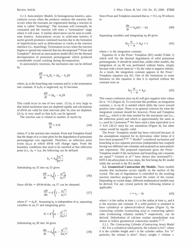
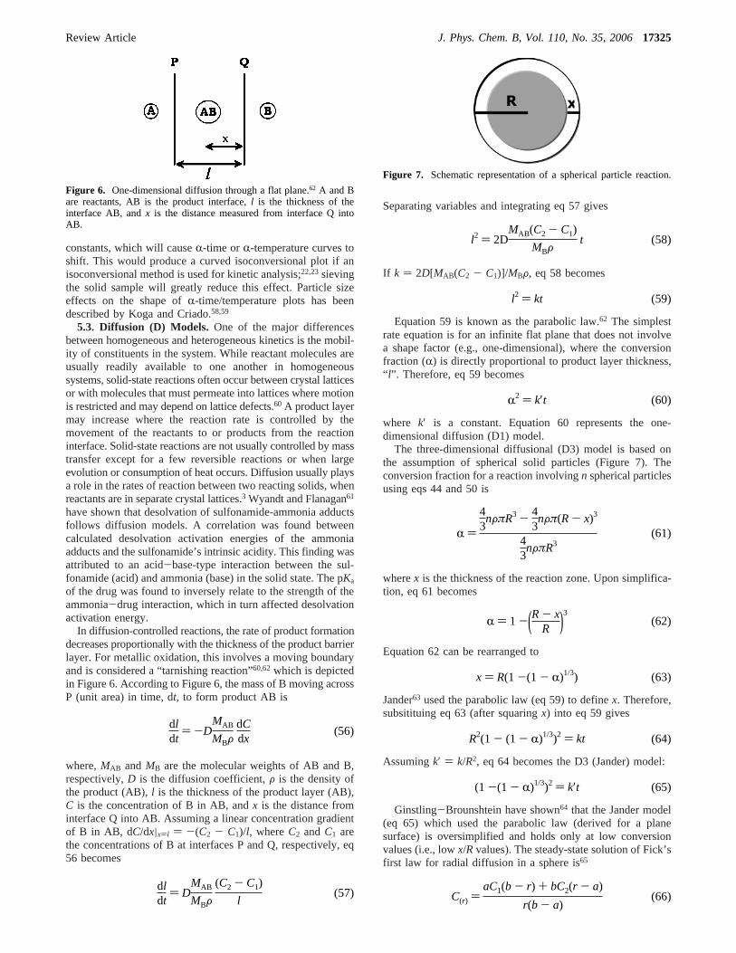
The three-dimensional diffusional (D3) model is based onthe assumption of spherical solid particles (Figure 7). Theconversion fraction for a reaction involvingn spherical particlesusing eqs 44 and 50 is

wherex is the thickness of the reaction zone. Upon simplifica-tion, eq 61 becomes

Equation 62 can be rearranged to

Jander63 used the parabolic law (eq 59) to definex. Therefore,subsitituing eq 63 (after squaringx) into eq 59 gives

Assumingk′ ) k/R2, eq 64 becomes the D3 (Jander) model:

Ginstling-Brounshtein have shown64 that the Jander model(eq 65) which used the parabolic law (derived for a planesurface) is oversimplified and holds only at low conversionvalues (i.e., lowx/Rvalues). The steady-state solution of Fick’sfirst law for radial diffusion in a sphere is65

Figure 6. One-dimensional diffusion through a flat plane.62 A and Bare reactants, AB is the product interface,l is the thickness of theinterface AB, andx is the distance measured from interface Q intoAB.

dldt

) -DMAB

MBFdCdx

(56)

dldt

) DMAB

MBF(C2 - C1)

l(57)

Figure 7. Schematic representation of a spherical particle reaction.

l2 ) 2DMAB(C2 - C1)

MBFt (58)

l2 ) kt (59)

R2 ) k′t (60)

R )

43nFπR3 - 4

3nFπ(R - x)3

43nFπR3

(61)

R ) 1 -(R - xR )3

(62)

x ) R(1 -(1 - R)1/3) (63)

R2(1 - (1 - R)1/3)2 ) kt (64)

(1 -(1 - R)1/3)2 ) k′t (65)

C(r) )aC1(b - r) + bC2(r - a)

r(b - a)(66)


whereC(r) is the reactant concentration at a particular value ofr (a < r < b), C1 is the concentration of the diffusing speciesat surfacer ) a, andC2 is the concentration of the diffusingspecies at surfacer ) b. The reaction at the interface is assumedto occur at a much faster rate than diffusion, therefore,C1 ≈ 0.Therefore, eq 66 becomes

Taking the derivative of the above equation with respect tor atr ) a gives

According to Figure 7,a ) R-x and b ) R, so that eq 68becomes

The rate of reaction zone advance, dx/dt, can be related to dC/dr by64

where D is the diffusion coefficient,ε is a proportionalityconstant equal toFn/µ (F and µ are the specific gravity andmolecular weight of the product, respectively, andn is thestoichiometric coefficient of the reaction). Subsituting eq 69into eq 70 gives

which can be rewritten as

wherek ) DC2/ε. Separating variables and integrating eq 72gives

Substituting forx in eq 73 with the value ofx in eq 63 andrearranging gives

Equation 74 is the Ginstling-Brounshtein (D4) model. The D4model is another type of three-dimensional model. Buscagliaand Milanese66 have proposed a generalized form of theGinstling-Brounshtein model and have discussed limitationsrelated to the boundary conditions for this model. The reactionbetween manganese oxide (Mn3O4) and sodium carbonate wasshown to follow the D4 model.67

If solid particles are assumed to be cylindrical, and diffusionoccurs radially through a cylindrical shell with an increasingreaction zone, a two-dimensional diffusion (D2) model can bederived. The D2 model can be derived using the same general

approach used for the D3 model. For a cylindrical particle, eq63 is defined as

If Jander’s approach is followed, the resulting equation is

where,k′ ) k/R2. Equation 76 is not the D2 model usually citedin the literature. The usual D2 model is derived following theGinstling-Brounshtein approach. The steady-state solution ofFick’s first law for radial diffusion in a cylinder is68

whereC(r) is the reactant concentration at a particular value ofr (a < r < b), C1 is the concentration of the diffusing speciesat surfacer ) a, andC2 is the concentration of the diffusingspecies at surfacer ) b. The reaction at the interface is assumedto occur at a much faster rate than diffusion, makingC1 ≈ 0.Therefore, eq 77 becomes

Taking the derivative of the above equation with respect tor at r ) a gives

According to Figure 8,a ) R-x andb ) R, therefore, eq 79becomes

Subsituting eq 80 into 70 gives

wherek ) DC2/ε. Substituting for the value ofx in eq 81 withx from eq 75 and rearranging gives

The derivative of eq 75 is

C(r) )bC2(r - a)

r(b - a)(67)

dCdr

|r)a )(b - a)bC2

a(b - a)2(68)

dCdr

)RC2

(R - x)x(69)

dxdt

) Dε

dCdr

(70)

dxdt

) Dε

RC2

(R - x)x(71)

dxdt

) kR

(Rx- x2)(72)

x2(12 - x3R) ) kt (73)

1 - 23R - (1 - R)2/3 ) kt (74)

Figure 8. Schematic representation of a cylindrical particle reaction.

x ) R(1 - (1 - R)1/2) (75)

(1 -(1 - R)1/2)2 ) k′t (76)

C(r) )C1ln(b/r) + C2ln(r/a)

ln(b/a)(77)

C(r) )C2ln(r/a)

ln(b/a)(78)

dCdr

|r)a )C2

aln(b/a)(79)

dCdr

)C2

(R - x) ln (R/(R - x))(80)

dxdt

) k(R - x) ln (R/(R - x))

(81)

dxdt

) - k

(1 - R)1/2 ln (1 - R)1/2(82)

dx ) R

2(1 - R)1/2dR (83)


Substituting eq 83 into eq 82 and rearranging gives

wherek′ ) 4k/R2. Equation 84 is the differential form of theD2 model. The integral form (Table 1) of the D2 model can beobtained by separating variables and integrating eq 84.

Finally, JMAEK models ((-ln [1 - R])1/n ) kt) have beenmodified to account for diffusion69 wheren becomes 1.5 (one-dimension), 2 (two-dimensions), and 2.5 (three-dimensions); thediffusion coefficient (D) is included in the reaction rate constant(k).

5.4. Order-Based (F) Models.Order-based models are thesimplest models as they are similar to those used in homoge-neous kinetics. In these models, the reaction rate is proportionalto concentration, amount or fraction remaining of reactant(s)raised to a particular power (integral or fractional) which is thereaction order. Some kinetic analysis methods force data intoan order-based model that may not be appropriate.4,27 Order-based models are derived from the following general equation

where dR/dt is the rate of reaction,k is the rate constant, andnis the reaction order.

If n ) 0 in eq 85, the zero-order model (F0/R1) model isobtained and eq 85 becomes

After separating variables and integrating, eq 86 becomes

If n ) 1 in eq 85, the first-order model (F1) model is obtainedand eq 85 becomes

Separating variables and integrating eq 88 leads to the first-order integral expression

The first-order model, also called the Mampel model,70,71 is aspecial case of the Avrami-Erofeyev (A) models wheren )1. Similarly, second-order (n ) 2) and third-order (n ) 3)models can be obtained (Table 1). Lopes et al.72 have shownthat decomposition of gadolinium(III) complexes follows a zero-order model. Thermal oxidation of porous silicon73 and desorp-tion of 2-phenylethylamine (PEA) from silica surfaces74 wereshown to follow a first-order model.

6. Summary

We have attempted to summarize the assumptions andmathematical derivation of the most commonly used reactionmodels in solid-state kinetics. This review has not beenexhaustive but rather representative of the common models used.Hopefully our presentation is a useful pedagogic tool forunderstanding solid-state kinetic models. Even though we havefocused on reactions involving weight loss (A(s)fB(s)+C(g)),many of the models are applicable to other solid-state reactionswhere, for example, evolution or consumption of heat is

measured. We hope that this work has demonstrated that solid-state kinetic models have a theoretical physical meaning andare not merely based on goodness of data fits to complexmathematical expressions.

Finally, investigators are challenged to better understand themodels and mathematical tools they apply to solid-state kineticreactions. We hope our work helps resolve some of the lack ofunderstanding of solid-state kinetic models.

References and Notes

(1) Chemistry of the solid state; Garner, W. E., Ed.; Academic Press:New York, 1955.

(2) Jacobs, P. W. M.; Tompkins, F. C. Classification and theory ofsolid reactions. InChemistry of the solid state; Garner, W. E., Ed.; AcademicPress: New York, 1955; Chapter 7.

(3) Brown, M. E.; Dollimore, D.; Galwey, A. K. Reactions in the solidstate. InComprehensiVe chemical kinetics; Bamford, C. H., Tipper, C. F.H., Eds.; Elsevier: Amsterdam, 1980; Vol. 22, Chapter 3.

(4) Galwey, A. K.; Brown, M. E.Thermal decomposition of ionicsolids: Chemical properties and reactiVities of ionic crystalline phases;Elsevier: Amsterdam, 1999; Chapter 3.

(5) Zhou, D. L.; Grant, D. J. W.J. Phys. Chem. A2004, 108, 4239.(6) Perez-Maqueda, L. A.; Criado, J. M.; Gotor, F. J.; Malek, J.J.

Phys. Chem. A2002, 106, 2862.(7) Gotor, F. J.; Criado, J. M.; Malek, J.; Koga, N.J. Phys. Chem. A

2000, 104, 10777.(8) MacNeil, D. D.; Dahn, J. R.J. Phys. Chem. A2001, 105, 4430.(9) Alkhamis, K. A.; Salem, M. S.; Obaidat, R. M.J. Pharm. Sci.2006,

95, 859.(10) Capart, R.; Khezami, L.; Burnham, A. K.Thermochim. Acta2004,

417, 79.(11) Khawam, A.; Flanagan, D. R.J. Pharm. Sci.2006, 95, 472.(12) Vyazovkin, S.; Dranca, I.J. Phys. Chem. B2005, 109, 18637.(13) Kirsch, B. L.; Richman, E. K.; Riley, A. E.; Tolbert, S. H.J. Phys.

Chem. B2004, 108, 12698.(14) Jones, A. R.; Winter, R.; Florian, P.; Massiot, D.J. Phys. Chem. B

2005, 109, 4324.(15) Bertmer, M.; Nieuwendaal, R. C.; Barnes, A. B.; Hayes, S. E.J.

Phys. Chem. B2006, 110, 6270.(16) Yu, Y. F.; Wang, M. H.; Gan, W. J.; Tao, Q. S.; Li, S. J.J. Phys.

Chem. B2004, 108, 6208.(17) Premkumar, T.; Govindarajan, S.; Coles, A. E.; Wight, C. A.J.

Phys. Chem. B2005, 109, 6126.(18) Bendall, J. S.; Ilie, A.; Welland, M. E.; Sloan, J.; Green, M. L. H.

J. Phys. Chem. B2006, 110, 6569.(19) Vyazovkin, S.; Dranca, I.J. Phys. Chem. B2004, 108, 11981.(20) Vyazovkin, S.; Dranca, I.; Fan, X. W.; Advincula, R.J. Phys. Chem.

B 2004, 108, 11672.(21) Milev, A. S.; McCutcheon, A.; Kannangara, G. S. K.; Wilson, M.

A.; Bandara, T. Y.J. Phys. Chem. B2005, 109, 17304.(22) Khawam, A.; Flanagan, D. R.Thermochim. Acta2005, 436, 101.(23) Khawam, A.; Flanagan, D. R.Thermochim. Acta2005, 429, 93.(24) Khawam, A.; Flanagan, D. R.J. Phys. Chem. B2005, 109, 10073.(25) Brown, M. E.J. Therm. Anal. Calorim.2005, 82, 665.(26) Brown, M. E.Introduction to thermal analysis: Techniques and

applications, 2nd ed.; Kluwer: Dordrecht, 2001; Chapter 10.(27) Vyazovkin, S.; Wight, C. A.Annu. ReV. Phys. Chem.1997, 48,

125.(28) Sestak, J.; Berggren, G.Thermochim. Acta1971, 3, 1.(29) Yang, J.; McCoy, B. J.; Madras, G.J. Phys. Chem. B2005, 109,

18550.(30) Yang, J.; McCoy, B. J.; Madras, G.J. Chem. Phys.2005, 122.(31) Liu, J.; Wang, J. J.; Li, H. H.; Shen, D. Y.; Zhang, J. M.; Ozaki,

Y.; Yan, S. K.J. Phys. Chem. B2006, 110, 738.(32) Burnham, A. K.; Weese, R. K.; Weeks, B. L.J. Phys. Chem. B

2004, 108, 19432.(33) Graetz, J.; Reilly, J. J.J. Phys. Chem. B2005, 109, 22181.(34) Wang, S.; Gao, Q. Y.; Wang, J. C.J. Phys. Chem. B2005, 109,

17281.(35) Hromadova, M.; Sokolova, R.; Pospisil, L.; Fanelli, N.J. Phys.

Chem. B2006, 110, 4869.(36) Wu, C. Z.; Wang, P.; Yao, X. D.; Liu, C.; Chen, D. M.; Lu, G. Q.;

Cheng, H. M.J. Phys. Chem. B2005, 109, 22217.(37) Peterson, V. K.; Neumann, D. A.; Livingston, R. A.J. Phys. Chem.

B 2005, 109, 14449.(38) Skrdla, P. J.; Robertson, R. T.J. Phys. Chem. B2005, 109, 10611.(39) Boldyrev, V. V.Thermochim. Acta1986, 100, 315.(40) Bagdassarian, C.Acta Physicochim. U.S.S.R.1945, 20, 441.(41) Allnatt, A. R.; Jacobs, P. W. M.Can. J. Chem.1968, 46, 111.

dRdt

) - k′ln(1 - R)

(84)

dRdt

) k(1 - R)n (85)

dRdt

) k (86)

R ) kt (87)

dRdt

) k(1 - R) (88)

-ln(1 - R) ) kt (89)


(42) Guo, L.; Radisic, A.; Searson, P. C.J. Phys. Chem. B2005, 109,24008.

(43) Avrami, M. J. Chem. Phys.1939, 7, 1103.(44) Avrami, M. J. Chem. Phys.1940, 8, 212.(45) Erofeyev, B. V.Dokl. Akad. Nauk SSSR1946, 52, 511.(46) Jacobs, P. W. M.J. Phys. Chem. B1997, 101, 10086.(47) Prout, E. G.; Tompkins, F. C.Trans. Faraday Soc.1944, 40, 488.(48) Carstensen, J. T.Drug stability: Principles and practices, 2nd

revised ed.; Marcel Dekker: New York, 1995; p. 237.(49) Brown, M. E.; Glass, B. D.Int. J. Pharm.1999, 190, 129.(50) Brown, M. E.Thermochim. Acta1997, 300, 93.(51) Prout, E. G.; Tompkins, F. C.Trans. Faraday Soc.1946, 42, 468.(52) Skrdla, P. J.J. Phys. Chem. A2004, 108, 6709.(53) Guinesi, L. S.; Ribeiro, C. A.; Crespi, M. S.; Santos, A. F.; Capela,

M. V. J. Therm. Anal. Calorim.2006, in press.(54) Carstensen, J. T.J. Pharm. Sci.1974, 63, 1.(55) Chunxiu, G.; Yufang, S.; Donghua, C.J. Therm. Anal. Calorim.

2004, 76, 203.(56) Liqing, L.; Donghua, C.J. Therm. Anal. Calorim.2004, 78, 283.(57) Gao, Z. M.; Amasaki, I.; Nakada, M.Thermochim. Acta2002, 385,

95.(58) Koga, N.; Criado, J. M.J. Am. Ceram. Soc.1998, 81, 2901.(59) Koga, N.; Criado, J. M.J. Therm. Anal.1997, 49, 1477.(60) Welch, A. J. E. Solid-solid reactions. InChemistry of the solid

state; Garner, W. E., Ed.; Academic Press: New York, 1955; Chapter 12.

(61) Wyandt, C. M.; Flanagan, D. R.Thermochim. Acta1992, 196, 379.(62) Booth, F.Trans. Faraday Soc.1948, 44, 796.(63) Jander, W.Z. Anorg. Allg. Chem.1927, 163, 1.(64) Ginstling, A. M.; Brounshtein, B. I.J. Appl. Chem. USSR1950,

23, 1327.(65) Crank, J.The mathematics of diffusion, 2nd ed.; Clarendon Press:

Oxford, England, 1975; Chapter 6, p 89.(66) Buscaglia, V.; Milanese, C.J. Phys. Chem. B2005, 109, 18475.(67) Eames, D. J.; Empie, H. J. International Chemical Recovery

Conference: Changing Recovery Technology to Meet the Challenges ofthe Pulp and Paper Industry, Whistler, BC, Canada, June 11-14, 2001.

(68) Crank, J.The mathematics of diffusion, 2nd ed.; Clarendon Press:Oxford, England, 1975; Chapter 5, p 69.

(69) Perez-Maqueda, L. A.; Criado, J. M.; Malek, J.J. Non-Cryst. Solids2003, 320, 84.

(70) Mampel, K. L.Z. Phys. Chem.1940, A187, 43.(71) Mampel, K. L.Z. Phys. Chem.1940, A187, 235.(72) Lopes, W. S.; Morais, C. R. D.; de Souza, A. G.; Leite, V. D.J.

Therm. Anal. Calorim.2005, 79, 343.(73) Pap, A. E.; Kordas, K.; George, T. F.; Leppavuori, S.J. Phys. Chem.

B 2004, 108, 12744.(74) Carniti, P.; Gervasini, A.; Bennici, S.J. Phys. Chem. B2005, 109,

1528.


Solid-State Kinetic Models

Documents

Transcript of Solid-State Kinetic Models