Solid Processing.pdf
188
SOLIDS PROCESSING 4200:461/561 Fall 2004 TABLE OF CONTENTS 1. INTRODUCTION 2. A CHEMICAL PROCESS INDUSTRY PERSPECTIVE 3. PROPERTIES OF PARTICULATE SOLIDS 4. BULK PROPERTIES OF SOLIDS 5. FLUIDIZATION 6. ELUTRIATION 7. SOLID/LIQUID SEPARATIONS 8. PRETREATMENT OF S/L MIXTURES 9. SEGREGATION MECHANISMS 10. HOPPER DESIGN 11. GRADE EFFICIENCY 12. CYCLONES 13. CONVEYING 14. DUST EXPLOSIONS
-
Upload
mahreza189 -
Category
Documents
-
view
144 -
download
7
description
Solid processing
Transcript of Solid Processing.pdf

SOLIDS PROCESSING
4200:461/561 Fall 2004
TABLE OF CONTENTS
1. INTRODUCTION
2. A CHEMICAL PROCESS INDUSTRY PERSPECTIVE
3. PROPERTIES OF PARTICULATE SOLIDS
4. BULK PROPERTIES OF SOLIDS
5. FLUIDIZATION
6. ELUTRIATION
7. SOLID/LIQUID SEPARATIONS
8. PRETREATMENT OF S/L MIXTURES
9. SEGREGATION MECHANISMS
10. HOPPER DESIGN
11. GRADE EFFICIENCY
12. CYCLONES
13. CONVEYING
14. DUST EXPLOSIONS

SOLIDS NOTES 1, George G. Chase, The University of Akron
1. INTRODUCTION
1.1 Organization of the Course Chapters 1 and 2 of this course give an introduction to this course with an emphasis on industrial applications. Chapters 3 and 4 introduce you to fundamental properties of particles and particulate systems. The remaining chapters cover specific topics such as conveying, hopper design, and separations.
For undergraduates this is a design course, hence you are expected to apply design methodology. You will be assigned laboratory projects to work on in which you will apply engineering judgment with design skills to produce a final product. Graduate students are required to write a paper concerning a particular aspect of solids processing.
There are two labs in this course. The labs are well defined and structured. A few class periods are dedicated to the labs, though you will probably have to spend some time out of class to complete the labs.
Depending on schedules and availablility, there may be a short field trip to tour a facility that handles bulk solids. Also, I may invite guest engineers to teach selected topics.
1.2 Acknowledgement I acknowledge engineer Karl Jacob, at the Dow Chemical Company at Midland Michigan, for his enthusiastic support in helping me prepare and organize this course. Karl introduced me to many of the topics used in pneumatic conveying and hopper design and helped write many of the notes.
I acknowledge the National Science Foundation GOALI grant CTS 9613904 for its financial support that made it possible for Karl Jacob and I to collaborate in developing this course.
Finally, I acknowledge the American Filtration and Separations Society and its members’ knowledge on a number of topics including particle size characterization, surface science and effects of surfactants, and various methods of fluid-particle separations. Many discussions with members of AFS over the past several years have helped me to refine my course notes and to focus on essential aspects of fluid/particle separations. The collective knowledge is vast and one course can only attempt to introduce students to selected topics.
1-2
SOLIDS NOTES 1, George G. Chase, The University of Akron
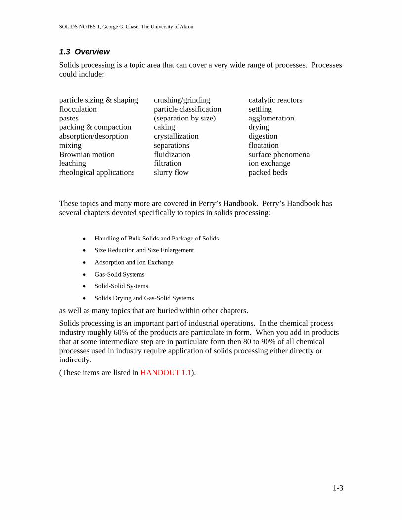
1.3 Overview Solids processing is a topic area that can cover a very wide range of processes. Processes could include:
particle sizing & shaping crushing/grinding catalytic reactors flocculation pastes
particle classification (separation by size)
settling agglomeration
packing & compaction caking drying absorption/desorption crystallization digestion mixing separations floatation Brownian motion fluidization surface phenomena leaching filtration ion exchange rheological applications slurry flow packed beds
These topics and many more are covered in Perry’s Handbook. Perry’s Handbook has several chapters devoted specifically to topics in solids processing:
• Handling of Bulk Solids and Package of Solids
• Size Reduction and Size Enlargement
• Adsorption and Ion Exchange
• Gas-Solid Systems
• Solid-Solid Systems
• Solids Drying and Gas-Solid Systems
as well as many topics that are buried within other chapters.
Solids processing is an important part of industrial operations. In the chemical process industry roughly 60% of the products are particulate in form. When you add in products that at some intermediate step are in particulate form then 80 to 90% of all chemical processes used in industry require application of solids processing either directly or indirectly.
(These items are listed in HANDOUT 1.1).
1-3

HANDOUT 1.1 Typical Solids Processing operations particle sizing & shaping crushing/grinding agglomeration flocculation particle classification (separation
by size) settling
packing & compaction caking drying absorption/desorption crystallization digestion mixing separations floatation Brownian motion fluidization surface phenomena leaching filtration ion exchange pastes slurry flow packed beds rheological applications catalytic reactors Sections in Perry’s Handbook
• Handling of Bulk Solids and Package of Solids • Size Reduction and Size Enlargement • Adsorption and Ion Exchange • Gas-Solid Systems • Solid-Solid Systems • Solids Drying and Gas-Solid Systems

SOLIDS NOTES 2, George G. Chase, The University of Akron
2. A CHEMICAL PROCESS INDUSTRY PERSPECTIVE
The chemical process industry makes heavy use of solids materials handling equipment and separations. Some examples from Shreve and Brink (see HANDOUT 2.1)
R.N. Shreve and J.A. Brink, Chemical Process Industries, 4th ed., McGraw-Hill, New York, 1977.
include process flow diagrams showing the materials handling and fluid/particle separations steps. Industries include:
water conditioning environmental cleanup coal chemicals glass industry industrial carbon phosphorous production ceramics potassium production paints nuclear industries explosives and propellants food and food processing agriculture sugar and starch fermentation wood chemicals pulp and paper plastics synthetic fibers rubber industries petrochemicals pharmaceuticals
A sampling of the process flow charts are in the 1977 publication, but for the most part these processes have not been altered significantly. In today's industries we could add other flow charts such as for terephthalic acid production for the polymer industry. However, many of the unit operations steps would be the same as shown in these flow charts.
The intent of showing you these flow charts is to make you aware of the important role that solids handling and fluid/solids separations have in the industrial operations. We are not going to go over each process in detail.
2-1
SOLIDS NOTES 2, George G. Chase, The University of Akron
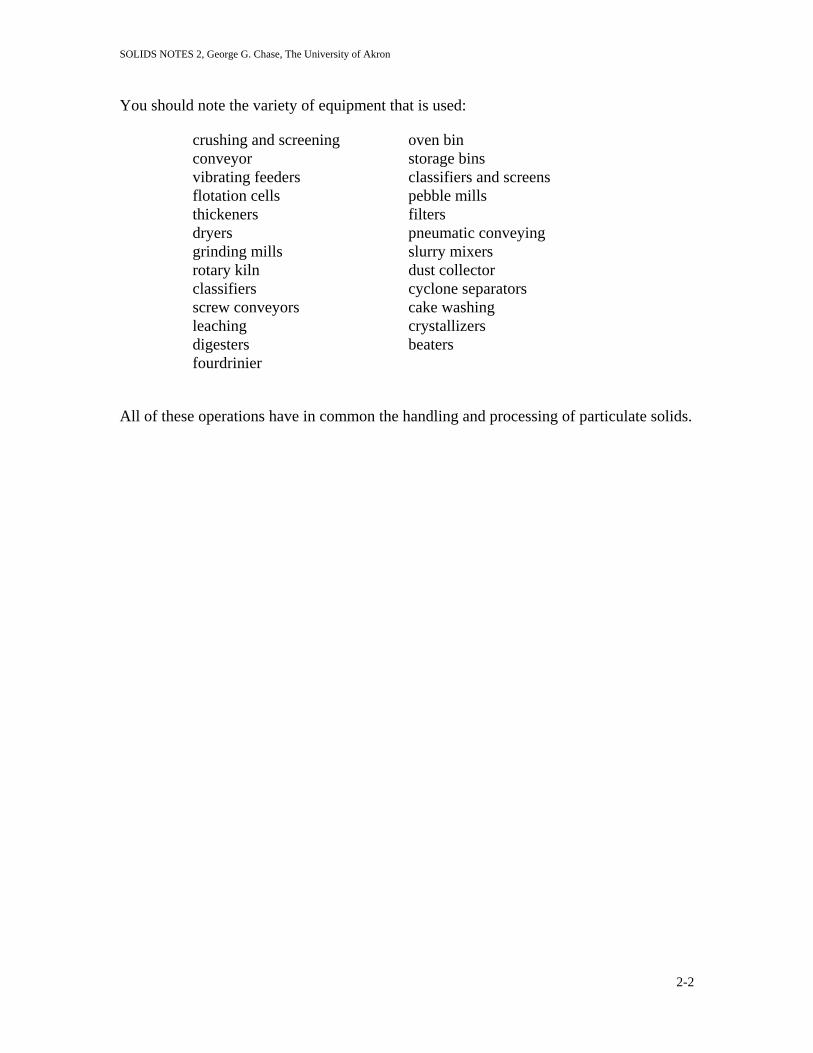
You should note the variety of equipment that is used:
crushing and screening oven bin conveyor storage bins vibrating feeders classifiers and screens flotation cells pebble mills thickeners filters dryers pneumatic conveying grinding mills slurry mixers rotary kiln dust collector classifiers cyclone separators screw conveyors cake washing leaching crystallizers digesters beaters fourdrinier
All of these operations have in common the handling and processing of particulate solids.
2-2

HANDOUT 2.1
R.N. Shreve and J.A. Brink, Chemical Process Industries, 4th ed., McGraw-Hill, New York, 1977.
PARTIAL LIST OF INDUSTRIES THAT USE FLUID/PARTICLE PROCESSES:
water conditioning environmental cleanup coal chemicals glass industry industrial carbon phosphorous production ceramics potassium production paints nuclear industries explosives and propellants food and food processing agriculture sugar and starch fermentation wood chemicals pulp and paper plastics synthetic fibers rubber industries petrochemicals pharmaceuticals
LIST OF OPERATIONS FOUND IN THE EXAMPLE INDUSTRIAL PROCESSES:
crushing and screening oven bin conveyor storage bins vibrating feeders classifiers and screens flotation cells pebble mills thickeners filters dryers pneumatic conveying grinding mills slurry mixers rotary kiln dust collector classifiers cyclone separators screw conveyors cake washing leaching crystallizers digesters beaters fourdrinier

SOLIDS NOTES 3, George G. Chase, The University of Akron
3. PROPERTIES OF PARTICULATE SOLIDS Before we can discuss operations for handling and separating fluid/particle systems we must understand the properties of the particles.
3.1 Individual particle characteristics In your assigned reading is a discussion on the characterization of particles. The way that we characterize the particles largely depends on the technique used to measure them.
The way that we measure a particle size is as important as the value of the measured size. For example, how would you quantify yourself if measured by
1. Circumference around your waist? 2. Diameter of a sphere of the same displacement volume as your body? 3. Length of your longest chord (height)?
As you can deduce, the measured values have different meanings and will be important relative to those meanings. If you are sizing a life jacket belt you would interested in the first size. If you are buying a sleeping bag I suggest the last one.
Based on the measurement techniques the particle sizes are typically related to equivalent sphere diameters by
a. The sphere of the same volume of the particle. b. The sphere of the same surface area as the particle. c. The sphere of the same surface area per unit volume. d. The sphere of the same area when projected on a plane normal to the direction
of motion. e. The sphere of the same projected area as viewed from above when lying in a
position of maximum stability (as with a microscope). f. The sphere which will just pass through the same size of square aperture as
the particle (as on a screen). g. The sphere with the same settling velocity as the particle in a specified fluid.
There are two other methods that I know of for sizing particles that are not based upon comparison to a standard (sphere) shape.
a. The first method is to fit the particle area projected shape to a polynomial type of relation. The values of the polynomial coefficients characterize the particle shape.
b. The second method is through the use of Fractals. A fractal length can be determined which characterizes the size of the particle and its dimensionality somewhere between linear and two-dimensional.
We will not be spending any time with these latter two methods though they would be interesting topics for a term paper. Sizes of common materials are listed in HANDOUT 3.1.
3-1

SOLIDS NOTES 3, George G. Chase, The University of Akron
Probably among the earliest forms of particle classification (sizing) to be developed is sieving. Several sieve standards exist which classify particles according to the size hole through which the particles can pass. Class HANDOUT 3.2 lists the Tyler and the US standard mesh nominal sizes as well as the screen opening sizes in mm and inches. Also in this handout is the Osmotics Inc. “Filtration Spectrum” which compares, among other things, the relative sizes of common materials.
Except for the extreme case of long thin fibers, the particle mean size will be of the same order of magnitude of the dimensions of the particle no matter which method is used.
There are a number of properties of particles that are of interest besides its size and shape. Particles can repel or attract each other due to static charge build up, they are affected by van der Waals forces (when they are small enough), they can stick, agglomerate, break up, bounce off of each other, chemically react with each other, and they are effected by the surrounding fluid phase due to drag an buoyant forces.
3.2 Measurements There are a number of methods for measuring particle sizes and size distributions. Many of these techniques are listed in HANDOUTS 3.3 and 3.4.
Some of these methods depend upon calibration with known particle sizes. A number of suppliers now sell small spherical particles of nearly uniform size distributions for calibration purposes.
Some of the more advanced methods of particle size measurement not only measure the particle sizes but they will also provide the size distributions of the particles. One of the better known instruments for this is the Coulter Counter. A brief description of the electronic particle counter principle is given in HANDOUT 3.5.
For a given material, there are four types of particle size distributions that are possible: (1) by number, (2) by length, (3) by surface, and (4) by mass (or volume).
Distributions can be reported either in terms of frequency (differential form) or by cumulative (integral form) as shown below.
To explain how we mathematically represent the distribution data, lets suppose that you measure the mass of particles by size by some unspecificed process. As an example your measured data may be plotted as shown in Figure 3-1. You can normalize the plot by dividing the masses of each size by the total mass, to obtain the mass fractions as shown in Figure 3-2.
Finally, if we add the mass fractions cumulatively we get the Cumulative Mass Fraction plot, shown in Figure 3-3.
3-2

SOLIDS NOTES 3, George G. Chase, The University of Akron
0
0.5
1
1.5
2
2.5
3
3.5
4
4.5
5
1 2 3 4 5
Diameter, x, mm
Mas
s, g
ram
s
Figure 3-1. Example mass quantities of a imaginary sample of particles.
0
0.1
0.2
0.3
0.4
0.5
0.6
0.7
0.8
0.9
1
1 2 3 4 5
Diameter, x, mm
Mas
s Fr
actio
n
Figure 3-2. Mass fractions from data in Figure 3-1.
3-3

SOLIDS NOTES 3, George G. Chase, The University of Akron
0
0.1
0.2
0.3
0.4
0.5
0.6
0.7
0.8
0.9
1
1 2 3 4 5
Diameter, x, mm
Cum
ulat
ive
Mas
s Fr
actio
n
Series5Series4Series3Series2Series1
Figure 3-3. Cumulative mass fraction plot of data from Figure 3-1.
From these Figures we see that the cumulatve mass fraction can be written mathematically as
(3-1) ∑=
∆=n
iimnm xFxF
0)()(
as a function of the nth particle size. Furthermore, we can write the increment in the cumulative mass, as mF∆
xxxF
xF imim ∆
∆∆
=∆)(
)( (3-2)
where x
Fm
∆∆
is the slope of the curve on the cumulative mass fraction plot. We define
this slope to be the frequency distribution of the mass fraction, , where mf
dx
dFxxF
xf mimim =
∆∆
=)(
)( . (3-3)
3-4

SOLIDS NOTES 3, George G. Chase, The University of Akron
Hence, we can relate the cumulative mass fraction to the frequency distribution by
∫
∑
∑
=
∆=
∆∆
∆=
=
=
nx
m
n
iim
n
i
imnm
dxf
xxf
xxxF
xF
0
0
0
)(
)()(
. (3-4)
Let the fractional amount of particles of size x be for any type of measurement (by mass, number, area, etc.) be represented as
(3-5) f x( ) = DISTRIBUTION FREQUENCY
(see L. Svarovsky, Solid-Liquid Separation, 3rd ed., Butterworth, London, 1990, chapter 2). If the particle size distribution is determined as the number fraction then the number frequency distribution is given by
particles ofnumber Total
xsize of particles ofNumber )( =∆xxfN . (3-6)
where is the differential range above and below size x that the number count represents. If the particle size distribution is determined on a microscope by measuring projected areas or by laser attenuation then the surface fraction or frequency distribution based on surface area is
x∆
particles all of area Total
xsize of particles all of Area)( =∆xxfs . (3-7)
Since f is a fractional amount, then integrating over all particle sizes gives the whole, or
(3-8) f x dx( )0
1∞
∫ =
and if we integrate over only the range from zero to some size x we get the cumulative fraction, F(x),
(3-9) F x f x dxx
( ) ( )= ∫0which is the area under the f(x) curve from 0 to x.
Plots of F and f have the general form
3-5

SOLIDS NOTES 3, George G. Chase, The University of Akron
0x
f or F
1
f(x)
F(x)
Figure 3-4. Typical f and F curves.
where f and F are also related by
f xdF x
dx( )
( )= (3-10)
The frequency distributions, f(x), and the cumulative fraction, F(x), may be based on numbers of particles or surface areas as described above, and are denoted with subscripts N or S. Linear and volume (mass) basis for the distributions also exist and are denoted by subscript L or M.
1. Number Distribution fN(x)
2. Distribution by Length fL(x) (Not used in practice)
3. Distribution by Surface fS(x)
4. Distribution by Mass fM(x) (Equivalent to distribution by volume)
The several types of distributions are all related to the number distribution by
(3-11) f x k x f xL ( ) ( )= 1 N
N
N
(3-12) f x k x f xS ( ) ( )= 22
(3-13) f x k x f xM ( ) ( )= 33
where k1, k2, and k3 are geometric shape factors.
Similarly, the cumulative distributions can be related
(3-14) ∑∫∫ ∆≅== xxfkdFxkdxxfxkxF N
x
N
x
NL 10 10 1 )()(
(3-15) ∑∫∫ ∆≅== xfxkdFxkdxxfxkxF N
x
N
x
NS2
20
220
22 )()(
. (3-16) ∑∫∫ ∆≅== xfxkdFxkdxxfxkxF N
x
N
x
NM3
30
330
33 )()(
3-6
SOLIDS NOTES 3, George G. Chase, The University of Akron
Often, experimental data are reported in discrete form (such as from a sieve analysis). For these data it is easier to work with discrete forms of the integral equations:
(3-17) j
i
jjNiN xxfxF ∆= ∑
=1
)()(
where j
jjN xN
nxf
∆=)( (3-18)
where is the number of particles in the jn jth set, N is the total number of particles, and
.is the size increment range that represents. jx∆ n j
As an example, to find k2, we start with
∑∑∑=
∆
∆==∆
jNj
jNj
jNj
jNj
jj
jjs Af
AfAxfN
AxfNAn
Anxf (assuming constant ). x∆
Let , and combine with Eq. (3-12), upon rearrangement we get 2jj xA π=
∑ ∆=
xfxk
Njj221 .
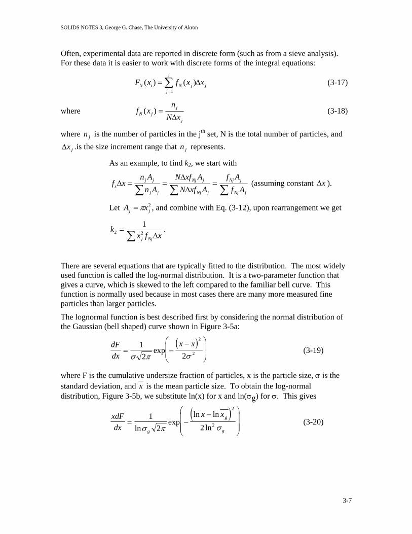
There are several equations that are typically fitted to the distribution. The most widely used function is called the log-normal distribution. It is a two-parameter function that gives a curve, which is skewed to the left compared to the familiar bell curve. This function is normally used because in most cases there are many more measured fine particles than larger particles.
The lognormal function is best described first by considering the normal distribution of the Gaussian (bell shaped) curve shown in Figure 3-5a:
( )dFdx
x x= −
−⎛
⎝⎜⎜
⎞
⎠⎟⎟
12 2
2
2σ π σexp (3-19)
where F is the cumulative undersize fraction of particles, x is the particle size, σ is the standard deviation, and x is the mean particle size. To obtain the log-normal distribution, Figure 3-5b, we substitute ln(x) for x and ln(σg) for σ. This gives
( )xdFdx
x x
g
g
g= −
−⎛
⎝
⎜⎜⎜
⎞
⎠
⎟⎟⎟
12 2
2
2lnexp
ln ln
lnσ π σ (3-20)
3-7
SOLIDS NOTES 3, George G. Chase, The University of Akron
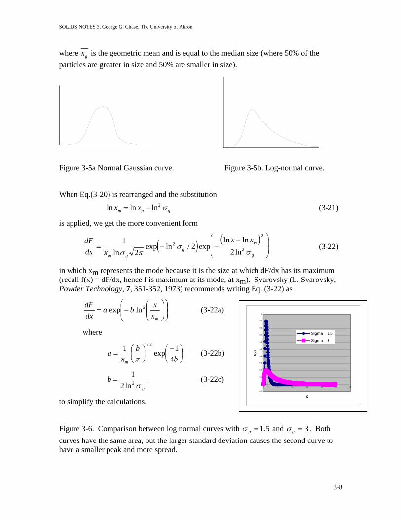
where xg is the geometric mean and is equal to the median size (where 50% of the particles are greater in size and 50% are smaller in size).
Figure 3-5a Normal Gaussian curve. Figure 3-5b. Log-normal curve.
When Eq.(3-20) is rearranged and the substitution
ln ln lnx xm g= − 2gσ (3-21)
is applied, we get the more convenient form
( ) ( )dFdx x
x x
m gg
m
g= − −
−⎛
⎝⎜⎜
⎞
⎠⎟⎟
12
22
2
2
2lnexp ln / exp
ln lnlnσ π
σσ
(3-22)
in which xm represents the mode because it is the size at which dF/dx has its maximum (recall f(x) = dF/dx, hence f is maximum at its mode, at xm). Svarovsky (L. Svarovsky, Powder Technology, 7, 351-352, 1973) recommends writing Eq. (3-22) as
⎟⎟⎠
⎞⎜⎜⎝
⎛⎟⎟⎠
⎞⎜⎜⎝
⎛−=
mxxba
dxdF 2lnexp (3-22a)
where
⎟⎠⎞
⎜⎝⎛ −
⎟⎠⎞
⎜⎝⎛=
bb
xa (3-22b)
m 41exp1 2/1
π
g
bσ2ln2
1= (3-22c)
1
to simplify the calculations.
Figure 3-6. Comparison between log normal curves withcurves have the same area, but the larger standard deviatiohave a smaller peak and more spread.
-0.1
0
0.1
0.2
0.3
0.4
0.5
0.6
0.7
0.8
0.9
0 5 10 15 20 25 30
X
f(x)
Sigma = 1.5
Sigma = 3
5.1=gσ and 3=gσ . Both n causes the second curve to
3-8

SOLIDS NOTES 3, George G. Chase, The University of Akron
EXAMPLE 3-1 (HANDOUT 3.6)
A sample of M&M’s ™ with peanuts are weighed as listed in Table 3-1. Using an average density of 1.23 grams per cubic centimeter, the average candy diameter (assuming spherical shape) is calculated. Plot the frequency distribution and the cumulative frequency distribution of the average diameter of the candies.
Table 3-1. Mass and diameter distribution of M&M’s.
Grams Dia, cm Size < Avg size No. fdx f F 2.06 1.473 1.5 1.475 1 0.047619 0.952381 0.0476192.18 1.501 2.18 1.501 2.21 1.508 2.22 1.511 2.35 1.540 2.36 1.542 2.37 1.544 1.55 1.525 7 0.333333 6.666667 0.380952
2.4 1.550 2.42 1.555 2.47 1.565 2.49 1.570 2.53 1.578 2.57 1.586 2.58 1.588 2.59 1.590 2.63 1.598 1.6 1.575 9 0.428571 8.571429 0.8095242.71 1.614 1.65 1.625 1 0.047619 0.952381 0.8571432.94 1.659 2.99 1.668 1.7 1.675 2 0.095238 1.904762 0.9523813.01 1.672 1.75 1.725 1 0.047619 0.952381 1
Total 21 1
Using the formulas in Eqs.(3-13) and (3-14) the frequency and cumulative frequency distributions are calculated. The particle sizes are added up in increments of 0.05 cm. The size ranges start with 1.45 to 1.50 cm. All M&Ms of size less than 1.50 are counted in the first increment, all M&Ms with size between 1.5 and 1.55 are in the second increment, and so on.
x∆
The values for nj are determined by counting the number of M&Ms that fall in a given size increment and are assigned to the average size in the increment.
For example, there are 7 M&Ms in the size increment range of 1.5 to 1.55 cm and are assigned to the average size of 1.525 cm.
fdx is determined by 7/21=0.33333, f is 0.33333/0.05 = 6.66667. F is determined by cumulative summing the values fdx.
Frequency Distribution of M&Ms
0
2
4
6
8
10
1.45 1.5 1.55 1.6 1.65 1.7 1.75
Diameter, cm
Freq
uenc
y D
istr
ibut
ion
0
0.2
0.4
0.6
0.8
1
fF
Figure 3-7. Plot of frequency and cumulative frequency distributions for M&M’s.
3-9

SOLIDS NOTES 3, George G. Chase, The University of Akron
The results of the summation are plotted in Figure 3-7.
3.3 Choice of Mean Particle Size As shown in handout 3 and the previous discussions, there is a bewildering number of different definitions of "mean" size for a particle. The choice of the most appropriate mean is vital in most applications.
As can be seen in Figure 3.8, two different size distributions may have the same arithmetic mean, but all of the other means may be different. (HANDOUT 3.7)
MODE HARMONIC MEAN
ARITHMETIC MEAN
MEDIAN f QUADRATIC MEAN
CUBIC MEAN
f x
Figure 3.8 Comparison of size distributions.
The mode is the x value at which f(x) is a maximum. The median is the x value at which F(x) = 0.50.
3-10

SOLIDS NOTES 3, George G. Chase, The University of Akron
The various means are defined by:
( ) ∫=1
0
)( dFxgxg (3-23)
or by the equivalent expressions
∫ ∑ ∆==1
0
)()()()()( xxfxgdxxfxgxg (3-24)
g(x) = NAME OF MEAN
x ARITHMETIC MEAN, ax
x2 QUADRATIC MEAN, qx
x3 CUBIC MEAN, cx
log x GEOMETRIC MEAN, gx
1/x HARMONIC MEAN, hx
Example, suppose we want the cubic mean of a set of particles for which we know the number distribution. The mean is defined such that
∑= iic nxNx 33,
or
∑ ∑ ∆== xfxNn
xx Niii
ic333
where Nn
xf iN =∆
hence
3 3∑ ∆= xfxx Niic
Suppose you have the mass distribution frequency of a set of particles and you want the geometric mean. How would you calculate the geometric mean from the given mass distribution frequency?
∑ ∆= xxfxx iMig )()log()log(
hence
3-11

SOLIDS NOTES 3, George G. Chase, The University of Akron
∑= ∆xxfxg
iMix )()log(10
The mean particle size is rarely quoted in isolation. It is usually related to some measurement technique and application and used as a single number to represent the full size distribution. The mean represents the particle size distribution by some property which is vital to the application or process under study. If two size distributions have the same mean (as measured using the same methods) then the behavior of the two materials are likely to behave in the process in the same way.
It is the application therefore which governs the selection of the most appropriate mean. Usually enough is known about a process to identify some fundamentals, which can be used as a starting point. The fundamental relations may be overly simple to describe the process fully, but it is better than randomly selecting mean definition.
EXAMPLE 3-2. Comparison of mass versus number count.
Consider measuring the size distribution by sieving. The results of a sieve analysis may give the size distribution as (HANDOUT 3.8)
Table 3.2 Sieve analysis of a sample of particles. Mass, number, and area fractions are calculated.
Sieve analysis of a sample of particles. Mass, number and area fractions are calculated. Note 1 Note 2
SIEVE AVG SIEVE MASS VOLUME ON VOLUME V1 NUMBER NUMBER A1
AREA TRAY AREA
SIZE, MM SIZE, MM
MASS,g FRAC
TRAY, MM^3 FRAC MM^3 FRAC MM^2 MM^2 FRAC
pan 0 0.04 0.05 0.10 0.03 38.46 0.03 0.00 67293.01 0.44 0.01 518.00 0.110.06 0.08 0.40 0.11 153.85 0.11 0.00 58141.16 0.38 0.02 1243.20 0.250.10 0.14 0.70 0.19 269.23 0.19 0.01 21045.58 0.14 0.06 1286.65 0.260.18 0.24 0.90 0.25 346.15 0.25 0.06 5660.10 0.04 0.17 982.00 0.200.30 0.36 0.70 0.19 269.23 0.19 0.21 1266.29 0.01 0.40 504.18 0.100.42 0.50 0.50 0.14 192.31 0.14 0.60 320.67 0.00 0.79 254.88 0.050.59 0.71 0.20 0.06 76.92 0.06 1.69 45.42 0.00 1.59 72.13 0.010.83 0.92 0.10 0.03 38.46 0.03 3.63 10.60 0.00 2.64 27.98 0.011.00
TOTAL MASS 3.60 1.00 1384.62 1.00 153782.82 1.00 4889.01 1.00
The mass fraction is found simply by dividing the sample masses (sieve mass) by the sum of the masses. Dividing the sample mass by the particle intrinsic density (assumed here to be 2.6 g/cm3) gives the volume of the particles in the sample. Dividing the sample volume by the volume of one particle ( 4
33π R ) where R is the sieve size opening, gives
3-12

SOLIDS NOTES 3, George G. Chase, The University of Akron
the number of particles for that sample. The total surface area of the particles of a given size is obtained by multiplying the number of particles times the surface area of one particle ( 4 ). The number and area fractions are found by dividing the sample values by the totals.
2π R
The plot in Figure 3.9 shows that the modes of the three distributions vary widely. The number distribution and surface area distribution are skewed greatly to the small particle size. This shows that a small mass of the fines contains a large number of particles.
A property such as turbidity is sensitive to the total number of particles, hence the large number of fines will cause the fluid to be cloudy. A process such as filtration is sensitive to the total surface area of the particles due to the drag resistance to flow across the surface.
0.00
0.05
0.10
0.15
0.20
0.25
0.30
0.35
0.40
0.45
0.50
0.00 0.20 0.40 0.60 0.80 1.00
Avg Particle Size, mm
Frac
tion Mass & Volume Frac
Number FracArea Frac
Figure 3.9. Comparison of the fractional distributions of the particle size distributions.
3-13

SOLIDS NOTES 3, George G. Chase, The University of Akron
EXAMPLE 3-3. Application: cake filtration, cake washing, dewatering, flow through packed beds and porous media.
If the particle size distribution is known, what definition of the mean should be used?
In flows through a packed bed we can consider the pores to be conduits. We can apply the concept of a friction factor and a Reynolds number. Since the geometry of an arbitrary pore is not cylindrical, we apply the hydraulic radius, Rh.
R
a
h =
=
=
⎛⎝⎜
⎞⎠⎟
⎛⎝⎜
⎞⎠⎟
=
cross - section area available for flowwetted perimeter
volume available for flowtotal wetted surface
volume of voidsvolume of bedwetted surfacevolume of bed
ε
(3-25)
where ε is the bed porosity and a is a surface area. This surface area is related to the specific surface area, as , of the solids (total particle surface/volume of particles) by
(a as= −1 )ε (3-26)
The specific surface area in turn is related to the mean particle diameter (assuming the particle can be represented by a sphere)
x Dap
s= = =
⋅6 6 total volume of particlestotal surface of particles
(3-27)
For spheres the total volume of particles is given by
( )total volume =
=
=
∑
∑
∑
43
1616
3
2
π
π
R
D D
x S
pi pi
i i
(3-28)
and the total surface area of the particles is given by
total surface area = = =∑ ∑ ∑42 2
π πR Di i Si (3-29)
Hence, we get the mean particle diameter to be
3-14
SOLIDS NOTES 3, George G. Chase, The University of Akron
x
x SS
xdF
i i
i
s
=
=
∑∑∫0
1 where
SS
dFi
is∑
= (3-30)
where the latter expression is the analytical formulation.
This latter expression defines the mean to be the arithmetic mean, ( )x xa s
= (from Eq. 3-23) of the distribution by surface.
Next, we must relate this to a size distribution by mass (the usual way of measurement). The surface distributions by surface and mass can be related by
( ) ( )f x kxf x
dFkx
m s
m
=
=
or
dFs
(3-31)
where k is a constant that accounts for the geometric shape of the particles. It is assumed here that k is independent of x.
Since the mean size is given in Eq. (3-30), then combining (3-30) and (3-31) we get
( )k
dFk
x msa11 1
0
== ∫ (3-32)
where the integral is unity. If we go back to Eq.3-31, we can integrate to obtain
∫∫ =1
0
1
0 kxdF
dF ms (3-33)
or, since k is not a function of x,
∫=1
0 xdF
k m (3-34)
where the RHS of Eq.(3-34) is the definition for the Harmonic mean,
( )1
xh m
, of the mass distribution given by Eq. (3-23). Hence this shows
that the surface arithmetic mean is equal to the mass harmonic mean, ( ) ( )x xa s h m
= .
Therefore, for flow through packed beds, filter cakes, etc., the appropriate mean particle size definition is the arithmetic average of the surface
3-15

SOLIDS NOTES 3, George G. Chase, The University of Akron
distribution. This is shown to be equivalent to the mass distribution harmonic mean.
EXAMPLE: 3-4. Mass recovery of solids in a dynamic separator such as a gravity settling tank.
For a settling process in which mass recovery is to be optimized, which would be the most appropriate mean particle size?
Total recovery of any separator can be obtained by combining the feed size cumulative distribution, F(x), with the operating grade efficiency curve, G(x). Mathematically, this is written as
(3-35) ∫=1
0
)( dFxGET
where Et is the recovery by mass.
A simple plug flow model of the separation in a settling tank without flocculation gives the grade efficiency in the form
G x u AQt( ) = (3-36)
where A is the settling area, Q is the suspension flow rate, and ut is the terminal velocity of particle size x.
Assuming Stoke's law for the terminal velocity
u xt =
2
18∆ρµ
g (3-37)
then these three equations can be combined to obtain
∫⋅∆
=1
0
2
18dFx
QgAEt µ
ρ (3-38)
where the integral defines the quadratic mean of the particle size distribution by mass.
We will discuss Grade Efficiency in further detail in a later section when we discuss separations processes.
3-16

SOLIDS NOTES 3, George G. Chase, The University of Akron
3.4 Drag Force on a Spherical Particle Probably the most significant force acting on particles in a fluid-particle medium is the drag force due to the relative motion between the fluid and the particles. A summary of the derivation of the governing equations is given here.
FMOVEMENTDIRECTION
F = m g
PARTICLE u
F = m gb f
g p
k
Figure 3-10. Free body diagram on particle of diameter R.
From a free body diagram, Figure 3.10, we can write a balance of forces acting on a spherical particle. The balance of forces shows that the accelerating force acting on the particle is given by
(3-39) F F F Fa g b= − − k
b
Initially, when a particle falls through a fluid the particle velocity accelerates. After a short distance the particle reaches its terminal velocity and its acceleration goes to zero. This means that the force of acceleration, Fa is zero.
Hence, at terminal velocity the kinetic force acting on the particle is given by
(3-40) F F Fk g= −
In Figure 3.10 mp is the mass of the particle and mf is the mass of the displaced fluid with the same volume as that of the particle. These masses are equal to the volume of the particle times the respective particle or fluid densities. The kinetic force becomes
( )F R gk =43
3π ρp − ρ (3-41)
We define the drag coefficient, Cd, by the expression
F C A KEk d= (3-42)
where A is the projected area normal to the flow and KE is the characteristic kinetic energy. When we substitute in the projected area of a sphere, πR2, and the kinetic energy, 1/2 ρu2, into Eq. (3-42) then we can derive a working equation for determining the drag coefficient as
( )
C RguD
p=
−83 2
ρ ρ
ρ (3-43)
In order to use this expression to determine values for CD we must run experiments. The experiments may be in the laboratory or they may be thought experiments for limiting case solutions.
Lets consider the limiting case of creeping flow around the sphere as shown in Figure 3.8. This operation is discussed in some detail by Bird et.al. (1960).
3-17

SOLIDS NOTES 3, George G. Chase, The University of Akron
v∞
X
r sin( )
y
φ θ x
r
θz
Z
Y
Figure 3-11. Flow around a sphere of radius R. The flow is in the positive z-direction such that there is symmetry in the φ-direction. At distances far from the sphere the flow velocity is uniform at a value v∞. This problem is equivalent to the particle falling in the negative z-direction through a stationary fluid.
For creeping flow the dominant term in the momentum balance is the viscous force term, which at the continuum scale gives
∇ ⋅ =τ 0 (3-44)
where the stress tensor is related to the velocity by the Newtonian Fluid model. Since the fluid motion around the sphere varies in the r- and θ-directions, it is mathematically easier to solve the resulting differential equations in terms of the stream function, ψ.
The stream function is related to the velocities in spherical coordinates by:
vrr = −
12 sinθ
∂ψ∂θ
(3-45)
vrθ θ r
∂ψ∂
= −1
sin (3-46)
In terms of the stream function, the momentum balance in spherical coordinates becomes:
∂∂
θ ∂∂θ θ
∂∂θ
ψr r+
⎛⎝⎜
⎞⎠⎟
⎡
⎣⎢
⎤
⎦⎥ =
sinsin2
21
0 (3-47)
where the [ ] term is a differential operator and where symmetry is assumed in the φ direction (hence no dependence on φ.
Equation (3-47) is solved with the boundary conditions
3-18

SOLIDS NOTES 3, George G. Chase, The University of Akron
vrr = − =
102 sinθ
∂ψ∂θ
at r = R (3-48)
vr rθ θ
∂ψ∂
= − =1
0sin
at r = R (3-49)
ψ θ→ − ∞12
2 2v r sin for r → ∞ (3-50)
The first two boundary conditions mathematically describe the contact of the fluid to the sphere surface. The third boundary condition shows that at distances far from the sphere the velocity becomes v∞.
The last boundary condition suggests that
(3-51) ψ = f r( ) sin2 θ
When this function is substituted into Eq.(3-47) we get the linear, homogeneous fourth-order equation
ddr r
ddr r
f r2
2 2
2
2 2
2 20−
⎛⎝⎜
⎞⎠⎟ −⎛⎝⎜
⎞⎠⎟ =( ) (3-52)
Assuming a solution of the form shows that n may have the values of -1,1,2,4 hence we get the functional form for f(r) as
f r Cr n( ) =
f rAr
Br Cr Dr( ) = + + +2 4 (3-53)
where A,B,C and D are constants.
Applying the boundary conditions and the definitions for the stream function (Eqs. (3-45)-(3-46) and (3-48)-(3-50)) gives the velocity profiles
θcos13
21
23
⎥⎥⎦
⎤
⎢⎢⎣
⎡⎟⎠⎞
⎜⎝⎛+−=
∞ rR
rR
vvr (3-54)
θθ sin13
41
43
⎥⎥⎦
⎤
⎢⎢⎣
⎡⎟⎠⎞
⎜⎝⎛−−−=
∞ rR
rR
vv (3-55)
We could derive an expression for the kinetic force on the sphere by using the momentum balances and an expression for the pressure distribution. A more direct way is to recognize that the drag force on the sphere is directly related to the viscous dissipation. For a Newtonian fluid, we can evaluate the kinetic or drag force directly using
v F v r dr d dkR
∞
∞
= − ∇⎛⎝⎜
⎞⎠⎟∫∫∫ τ θ θ φ
ππ
: sin2
00
2
(3-56)
Insertion of Newton’s Law of viscosity for the stress tensor in Eq.(3.41) and substitution of the velocity profiles in Eqs.(3.39) and (3.40) yields the kinetic force as
3-19
SOLIDS NOTES 3, George G. Chase, The University of Akron
F vk = ∞6 Rπ µ (3-57)
This expression is known as Stoke's Law. Defining the Reynold's number as
Rd v
ep
=∞ρµ
(3-58)
where is the particle diameter, we seek a correlation to relate the drag force to the Reynold's number. A correlation would allow us to extend our applications to flow conditions in which the creeping flow solution does not apply.
d p
The drag coefficient, Cd, defined by expression (3-42) may be combined with Eqs.(3-57) and (3-58) to derive
C (3-59)
0.1
1
10
100
1000
10000
100000
0.001 0.01 0.1 1 10 100 1000 10000 100000
Re
Cd
Expl curveStokesIntermediateNewton Law
Rdep
=24
Rep Rep
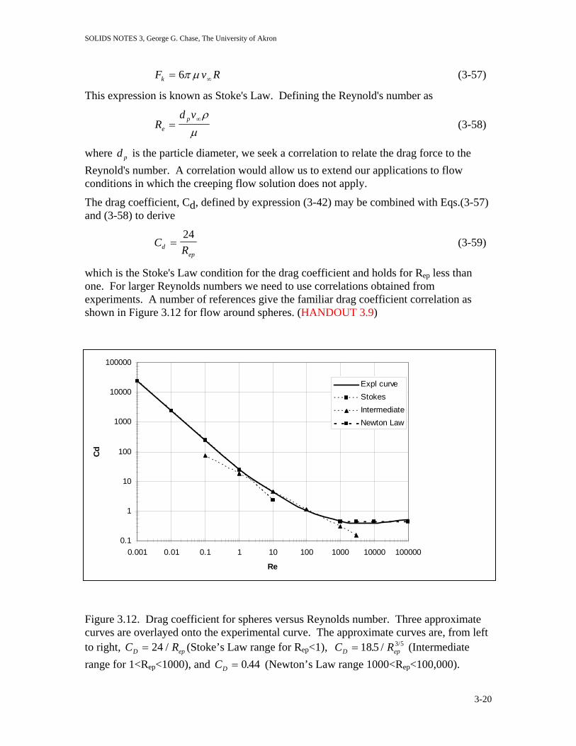
which is the Stoke's Law condition for the drag coefficient and holds for Rep less than one. For larger Reynolds numbers we need to use correlations obtained from experiments. A number of references give the familiar drag coefficient correlation as shown in Figure 3.12 for flow around spheres. (HANDOUT 3.9)
Figure 3.12. Drag coefficient for spheres versus Reynolds number. Three approximate curves are overlayed onto the experimental curve. The approximate curves are, from left to right, C (Stoke’s Law range for RD = 24 / ep<1), (Intermediate range for 1<R
CD = 18 5 3 5. / /
ep<1000), and CD = 0 44. (Newton’s Law range 1000<Rep<100,000).
3-20
SOLIDS NOTES 3, George G. Chase, The University of Akron
For Reynold’s numbers less than 1 Stokes Law applies and this is known as Stoke’s Law range. For Reynolds numbers greater than about 1000 and less than 105, where CD is a constant, this is known and Newton’s Law range. Between these two ranges is known as the intermediate range.
As can be seen in Figure 3.4 of the text by Coulson and Richardson (Chemical Engineering, Vol. 2, 4th ed, Pergamon, 1991), above Rep of about 105 there is a sudden decrease in the drag coefficient. In the book notation Re’=Rep and 2Cd=R’/ρu2. Rep >105 we get Cd=0.08.
Figures 3.2 and 3.3 in Coulson and Richardson (ibid) show the transition from smooth, well behaved laminar flow (Stoke’s regime), into the turbulent ranges and the formation of fluid eddies as the boundary layer separates from the particle surface. At the highest flow range new mechanisms can become important as the fluid separates away from the particle surface and cause the observed decrease in the drag coefficient.
If we rearrange Eq.(3-43) we can solve for the terminal velocity of the particle to be
ud gCt
p
D
p=
−⎛⎝⎜
⎞⎠⎟4
3
ρ ρρ
(3-60)
which applies to all flow regimes. When we substitute in Stoke’s Law, Eq.(3-60), we get the terminal velocity to be
( )
ugd
tp p
=−2
18
ρ ρ
µ (3-61)
in Stoke’s Law range. Similarly in Newton’s Law range substitution of CD = 0.44 yields
( )
ud g
t
p p=
−173.
ρ ρ
ρ (3-62)
Literature references have other correlations for representing these various ranges of Reynolds numbers.
These correlations only relate the motion to a few of the important factors (density, size, Reynold’s number). There are many other factors that may become significant in given situations. These include
• proximity to vessel walls • particle surface roughness • particle shape • Brownian motion (for dp < 1 µm) • external forces (electrical current, magnetic fields) • sound waves • rigid vs. deformable particles (ie., droplets) • particle concentration
The last topic in the list will be discussed further in a later section.
3-21

SOLIDS NOTES 3, George G. Chase, The University of Akron
3.5 Drag Force on Non-Spherical Particles The shape and orientation of the particle has an important effect on the flow profiles around the particle. McCabe and Smith (Unit Operations of Chemical Engineering, 6th ed, McGraw-Hill, N.Y., 2001), Figure 7.3, and Perry’s Chemical Engineer’s Handbook, (6th ed., McGraw-Hill, N.Y., 1984) Figure 5-76) show the correlation for the drag coefficients for spheres, disks, and cylinders.
It is not practical to try to derive correlations for all particle shapes and orientations, especially when in the chemical process industry particles in settling operations tumble and rotate.
Kunii and Levenspeil studied this problem and developed a correlation based upon sphericity (1966).
Sphericity is a measure of how close a particle is to being a sphere defined as
Φ =surface area of a sphere with same volume as the particle
actual surface area of the particle (3-63)
The sphericity of some common materials are given in Table 3.3. (HANDOUT 3.10).
Table 3-3 Sphericity of Some Common Materials (McCabe & Smith, 6th ed, pg945; Perry’s Handbook 6th ed, pg 5-54).
PARTICLE MATERIAL SPHERICITY Sphere 1.0 Cube 0.81 Short Cylinder (Length=Diameter) 0.87 Berl saddles 0.3 Raschig rings 0.3 Coal dust, natural (up to 3/8 inch) 0.65 Glass, crushed 0.65 Mica flakes 0.28 Sand
Average for various types Flint sand, jagged Sand, rounded Wilcox sand, jagged
0.75 0.65 0.83 0.6
Most crushed materials 0.6 to 0.8
Kunii and Levenspiel (Fluidization Engineering, John Wiley, N.Y. 1969, pg 77) took data from Brown (G.G. Brown et.al., Unit Operations, John Wiley, N.Y., 1950) and calculated the relationships plotted in Figure 3-10, HANDOUT 3.11, relating Cd to Rep.
3-22

SOLIDS NOTES 3, George G. Chase, The University of Akron
It turns out that the product C R is independent of velocity, which makes it convenient for calculations. Using Eq.(3-43) and the definition of the Reynold’s Number we get
d ep2
( )
( )
GA
pp
ppepd
N
gd
udu
RgRC
34
2
3
34
2
2382
=
−=
⎟⎟⎠
⎞⎜⎜⎝
⎛⎟⎟⎠
⎞⎜⎜⎝
⎛ −=
µρρρ
µρ
ρρρ
(3-64)
where ( )2
3
µρρρ −
= sGA
gdN (3-65)
is known as the Galileo number. With this chart and the correlation in Eq. (3-64) the terminal velocity can be calculated from the material properties and the sphericity.
1.E+00
1.E+01
1.E+02
1.E+03
1.E+04
1.E+05
1.E+06
1.E+07
1.E+08
1.E+09
1.E+10
1.E-01 1.E+00 1.E+01 1.E+02 1.E+03 1.E+04
Rep
SPHERICITY
0.80.6
1.0
0.40.2
Plot to determine drag coefficients of irregularly shaped particles at terminal velocity. The particles are randomly oriented relative to the flow direction. Shape is accounted for by the sphericity.
Figure 3-13. Drag coefficient – Reynolds number relationship for non-spherical particles. Equations 3-54, 3-60, and 3-61 are used with this chart. The particle diameter is the volume equivalent diameter, xv, of the sphere with the same volume as the particle.
3-23

SOLIDS NOTES 3, George G. Chase, The University of Akron
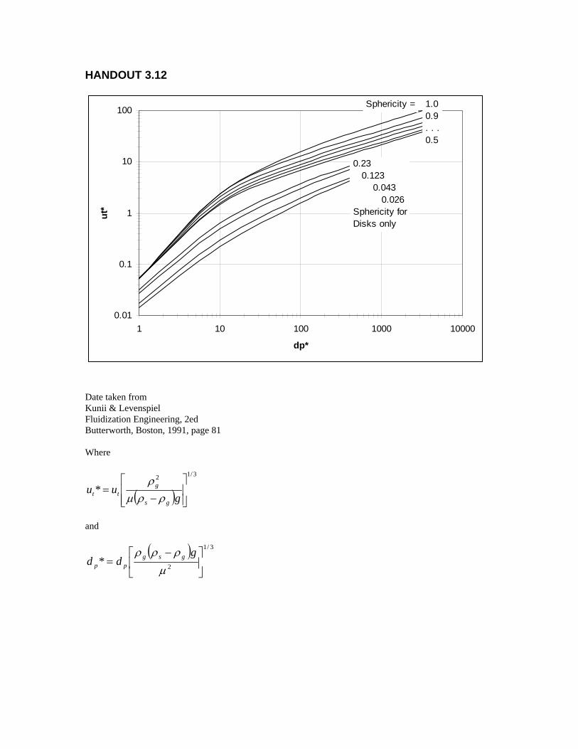
Haider and Levenspeil (Powder Technology, 58, 63, 1989) also found a useful relationship for direct evaluation of terminal velocity of particles. The correlation is shown in Figure 3-14 (HANDOUT 3.12) where a curve fit of the plot gives
ud dt
p p
** * .
. .. .= +
−⎡
⎣⎢⎢
⎤
⎦⎥⎥
< <
−18 2 335 1744
05 102 0 5
1Φ
Φ for (3-66)
and the dimensionless velocity and particle diameter are defined as
( )u ug
t t
p
*
/
=−
⎡
⎣
⎢⎢
⎤
⎦
⎥⎥
ρ
µ ρ ρ
21 3
(3-67)
and ( )
d dg
p p
p*
/
=−⎡
⎣
⎢⎢
⎤
⎦
⎥⎥
ρ ρ ρ
µ 2
1 3
. (3-68)
0.01
0.1
1
10
100
1 10 100 1000 10000
dp*
ut*
Sphericity = 1.00.9. . . 0.5
0.23 0.123 0.043 0.026Sphericity forDisks only
Figure 3-14. Plot of data taken from Kunii and Levenspiel, Fluidization Engineering, 2nd, Butterworth, Boston, 1991. Dimensionless terminal velocity and particle diameter are defined in Eqs.(3-67) and (3-68).
3-24

SOLIDS NOTES 3, George G. Chase, The University of Akron
EXAMPLE 3-5. Compare the terminal velocity of a cube of titanium, 5mm on each side, falling through maple syrup and falling through water. Properties: titanium density = 7.14 g/cc; syrup density = 0.95 g/cc, syrup viscosity = 3000 cP; water density = 1.0 g/cc, water viscosity = 1.0 cP.
SOLUTION:
For a cube . Since settling depends upon mass average of the particle size, then the appropriate diameter is that of a sphere of the same volume.
Φ = 081.
393
33 101251000
)5( mxmm
mmmlvolume −=⎟⎠⎞
⎜⎝⎛==
d x m xp = =− −6125 10 6 20 109 33 3
π. m
For the syrup:
( )d x m
g cc g cckg
gcm
mm s
cPkg
mscP
p*
/
.( . / ) . . / ( . / )
( )
.
=−
⎛⎝⎜
⎞⎠⎟⎛⎝⎜
⎞⎠⎟
⎛⎝⎜
⎞⎠⎟
⎡
⎣
⎢⎢⎢⎢⎢
⎤
⎦
⎥⎥⎥⎥⎥
=
−
−
6 20 100 95 7 14 0 95
1000100
9 807
3000 10
115
3
22 6
2
2 3
2
1 3
[ ]
u ug cc
kgg
cmm
cPkg
mscPg cc m s
u s m
t t
t
*
/
( . / )
( ) ( . . / )( . / )
. /
=
⎛⎝⎜
⎞⎠⎟⎛⎝⎜
⎞⎠⎟
⎛⎝⎜
⎞⎠⎟ −
⎡
⎣
⎢⎢⎢⎢⎢
⎤
⎦
⎥⎥⎥⎥⎥
=
−
0 951000
100
3000 10 7 14 0 95 9 807
170
23
3 2
1 3
From the figure u hence t* .= 0 07 u
s mm st = =
0 07170
0 041.
. /. / .
Similarly for the water
[ ]u u s mt t* . /= 2551
d p* = 243
and from the figure hence ut* = 17 u mt s= 0 67. / .
This shows that a change of 3000x in viscosity produces about a 10x change in the terminal velocity.
3-25

SOLIDS NOTES 3, George G. Chase, The University of Akron
More on Sphericity:
We represent a bed of non-spherical particles by a bed of spheres of diameter such that a bed of spheres and a bed of non-spheres have
Deff
• The same total surface area, in a given volume of the bed. a
• The same fractional voidage, εbed .
This representation ensures almost the same flow resistance in both beds.
In typical use of the Ergun Equation (McCabe & Smith), the effective diameter of the particle is replaced with the sphericity times the defined diameter based on sphericity;
. D Deff sph= Φ
The sphecific surface area of particles in either bed is found to be
a
D
D
s
sph
sph
=⎛⎝⎜
⎞⎠⎟
=
Surface area of one particlevolme of one particle
=Dsph
2ππ
//Φ
Φ
3 66
(3-69)
For the whole bed
aDsph
=⎛⎝⎜
⎞⎠⎟ =
−Surface of all particlesTotal volume of particles in the bed
6 1( )εΦ
(3-70)
Since there is no general relationship between and (particle diameter corresponding to a sphere of the same volume), the best we can do without running experiments is as follows:
Deff d p
• For irregular particles with no seemingly longer or shorter dimensions (hence isotropic in irregular shape)
D Deff sph p= d=Φ Φ (3-71)
• For irregular particles with one longer direction , but with a length ratio not greater than 2:1 (eggs for example)
D Deff sph p= d=Φ (3-72)
• For irregular particles with one dimension shorter, but with a length ratio not less than 1:2 (peanut, for example)
(3-73) D Deff sph p= =Φ Φ 2d
• For very flat or needlelike particles, estimate the relationship between and from Φ values for corresponding disks and cylinders.
d p
Deff
3-26

HANDOUT 3.1
1 Angstrom
1 Nanometer
1 Micron
1 Millimeter
1
10
100
10001
10
100
10001
10
100 APPROX.MOLEC.WT.
100
200
20k
200k
AQUEOUSSALTS
CARBONBLACK
PAINTPIGMENT
BACTERIAYEAST CELLS
PROTEINALBUMIN
TALCCLAY
RED BLOODCELLS
POLLEN
HUMAN HAIR
PARTICLEFILTRATION
MICROFILTRATION
ULTRAFILTRATION
REVERSEOSMOSIS
RANGEPARTICLE
MATERIALSCOMMON
PROCESSSEPARATION
LOG SCALEPARTICLE SIZE
MO
LECU
LAR
Ultraviolet
X-rays
SPECTRUMMAGNETICELECTRO-
0
1
2
3IO
NIC
MO
LECU
LEM
ACR O
Infrared
Radio waves
7
4
5
6
8
MAC
ROVisible
MIC
ROCOLLOIDAL
MIC
ROSC
OPE
ATOMS
METAL IONS
SUGARS
VIRUS
SILICA
ELEC
TRO
NM
ICRO
SCO
PEPYROGEN
TOBACCO SMOKE
BEACHSAND
GRAVEL
VISI
BLE
TO E
Y EO
PTIC
AL
DUSTMILLEDFLOUR
COAL
-LUCITE-GEON-ETC.
POLYMERPOWDERS

HANDOUT 3.2
STANDARD MESH SIZE
Tyler US mm Inches
4 4 4.70 0.185
6 6 3.33 0.131
8 8 2.36 0.094
10 12 1.65 0.065
12 14 1.40 0.056
14 16 1.17 0.047
16 18 0.991 0.039
20 20 0.833 0.033
24 25 0.701 0.028
28 30 0.589 0.023
32 35 0.495 0.020
35 40 0.417 0.016
42 45 0.351 0.014
48 50 0.295 0.012
60 60 0.246 0.0097
80 80 0.175 0.0069
100 100 0.147 0.0058
150 140 0.104 0.0041
200 200 0.074 0.0029
250 230 0.061 0.0024
325 325 0.043 0.0017
400 400 0.038 0.0015

HANDOUT 3.3 Taken from Tables 2.1, 2.2, 2.3, and 2.7 in L. Svarovsky, Solid-Liquid Separation, 3rd Ed., Butterworths, London, 1990. DEFINITIONS OF EQUIVALENT AND STATISTICAL DIAMETERS. Symbol Name Definition
DEFINITIONS OF EQUIVALENT SPHERE DIAMETERS xv Volume diameter Diameter of sphere with the same volume as the particle. xs Surface diameter Diameter of sphere with the same surface area as the particle. xd Drag diameter Diameter of sphere that has the same resistance to motions at the
same velocity as the particle. xf Free-falling diameter Diameter of sphere of same density as the particle with the same
free-falling speed in the same liquid. xSt Stoke’s diameter Same as xf but for when Stoke’s Law applies (Re < 0.2) xA Sieve diameter Largest diameter sphere that can pass through the square aperture
of the sieve screen. xSV Surface to Volume Ratio Diameter of sphere that has the same surface area to volume ratio
as the particle. DEFINITIONS OF EQUIVALENT CIRCLE DIAMETERS
xz Projected area diameter Projected area if the particle is resting in a stable position. xp Projected area diameter Projected area if the particle is randomly oriented. xc Perimeter diameter Diameter of a sphere with the same projected perimeter as the
perimeter of the projected outline of the particle. DEFINITIONS OF STATISTICAL DIAMETERS
xF Feret’s diameter Distance between two tangents on opposite sides of the particle. xM Martin’s diameter Length of the line which bisects the projected image of the particle
(the two halves of the image have equal areas). xSH Shear diameter Particle width obtained with an image shearing eyepiece. xCH Maximum chord
diameter Maximum length of a line limited by the contour of the projected image of the particle.

HANDOUT 3.4 LABORATORY METHODS OF PARTICLE SIZE MEASUREMENTS METHOD APPROX
SIZE, µm SIZE TYPE TYPE OF SIZE
DISTRIBUTION Sieving (wet or dry) Woven wire Electro formed
37-4000 5-120
xA By mass
Microscopy Optical Electron
0.8 – 150 0.001 – 5
xz, xF, xMxSH, xCH
By number
Gravity sedimentation 2-100 xSt, xf By mass Centrifugal sedimentation 0.01 - 10 xSt, xf By mass Flow Classification Gravity elutriation (dry) Centrifugal elutriation (dry) Impactors (dry) Cyclonic (wet or dry)
5 - 100 2 - 50 0.3 – 50 5 - 50
xSt, xf By mass By mass By mass or by number By mass
Coulter principle (elect. resist.) 0.8 – 200 xv By number Field flow fractionation 0.001 – 100 xd Depends upon detector Hydrodynamic chromatography 0.01 – 50 xd Depends upon detector Fraunhofer diffraction (laser) 1 – 2000 Equiv laser diameter By volume Mie theory light scattering (laser) 0.1 – 40 Equiv laser diameter By volume Photon correlations spectroscopy 0.003 – 3 Equiv laser diameter By number Scanning infrared laser 3 – 100 Chord length By number Aerodynamic sizing nozzle flow 0.5 – 30 xd By number Mesh obscurtion method 5 – 25 xA By number Laser Doppler phase shift 1 – 10,000 Equiv laser diameter Mean only Time of transition 150 – 1200 Equiv laser diameter By number Surface area to volume ratio Permeametry Hindered settling Gas diffusion Gas adsorption Adsorption from solution Flow microcalorimetry
Calculated xSV By number mean

HANDOUT 3.5
ELECTRONIC PARTICLE COUNTER The electronic particle counters can measure particle sizes ranging from 0.4 to 1200 micrometers. This method requires the particles to be placed in a stirred electrolyte solution. The resistance to the flow of electrical current through a small aperture is calibrated to the change in resistance depending upon the particle size (Figure 1).
Figure 1. Basic components of the Coulter Counter.
As the particles pass through the aperture opening, they bend the current flux lines around the particles, thus causing a longer length for the current to pass and thus a higher resistance to the current (Figure 2). Voltage and current are measured to quantify the resistance using Ohm’s Law: V = IR.
APERTURE OPENING APERTURE OPENING WITHOUT PARTICLE WITH PARTICLE
Figure 2. Particles in the aperture bend the electrical current flux lines.

HANDOUT 3.6 EXAMPLE 3-1 A sample of M&M’s ™ with peanuts are weighed as listed in Table 3-1. Using an average density of 1.23 grams per cubic centimeter, the average candy diameter (assuming spherical shape) is calculated. Plot the frequency distribution and the cumulative frequency distribution of the average diameter of the candies. Using the formulas in Eqs.(3-13) and (3-14) the frequency and cumulative frequency distributions are calculated. The particle sizes are added up in increments of 0.05 cm. The size ranges start with 1.45 to 1.50 cm. All M&Ms of size less than 1.50 are counted in the first increment, all M&Ms with size between 1.5 and 1.55 are in the second increment, and so on.
x∆
The values for nj are determined by counting the number of M&Ms that fall in a given size increment and are assigned to the average size in the increment. For example, there are 7 M&Ms in the size increment range of 1.5 to 1.55 cm and are assigned to the average size of 1.525 cm. fdx is determined by 7/21=0.33333, f is 0.33333/0.05 = 6.66667. F is determined by cumulative summing the values fdx. The results of the summation are plotted in Figure 3-4.
Table 3-1. Mass and diameter distribution of M&M’s.
Grams Dia, cm Size < Avg size No. fdx f F 2.06 1.473 1.5 1.475 1 0.047619 0.952381 0.0476192.18 1.501 2.18 1.501 2.21 1.508 2.22 1.511 2.35 1.540 2.36 1.542 2.37 1.544 1.55 1.525 7 0.333333 6.666667 0.380952
2.4 1.550 2.42 1.555 2.47 1.565 2.49 1.570 2.53 1.578 2.57 1.586 2.58 1.588 2.59 1.590 2.63 1.598 1.6 1.575 9 0.428571 8.571429 0.8095242.71 1.614 1.65 1.625 1 0.047619 0.952381 0.8571432.94 1.659 2.99 1.668 1.7 1.675 2 0.095238 1.904762 0.9523813.01 1.672 1.75 1.725 1 0.047619 0.952381 1
Frequency Distribution of M&Ms
0
2
4
6
8
10
1.45 1.5 1.55 1.6 1.65 1.7 1.75
Diameter, cm
Freq
uenc
y D
istr
ibut
ion
0
0.2
0.4
0.6
0.8
1
fF
Figure 3-4. Plot of frequency and cumulative frequency distributions for M&M’s.

HANDOUT 3.7 MODE HARMONIC MEAN
ARITHMETIC MEAN
MEDIAN f QUADRATIC MEAN
CUBIC MEAN
f x
Figure 3.5. Comparison of mean size distributions where the various means are defined by:
( )g x g x dF= ∫ ( )0
1
g(x) = NAME OF MEAN
x ARITHMETIC MEAN, ax
x2 QUADRATIC MEAN, qx
x3 CUBIC MEAN, cx
log x GEOMETRIC MEAN, gx
1/x HARMONIC MEAN, hx

HANDOUT 3.8 Sieve analysis of a sample of particles. Mass, number, and area fractions are calculated.
Sieve analysis of a sample of particles. Mass, number and area fractions are calculated. Note 1 Note 2
SIEVE AVG SIEVE MASS VOLUME ON VOLUME V1 NUMBER NUMBER A1
AREA TRAY AREA
SIZE, MM SIZE, MM
MASS,g FRAC
TRAY, MM^3 FRAC MM^3 FRAC MM^2 MM^2 FRAC
pan 0 0.04 0.05 0.10 0.03 38.46 0.03 0.00 67293.01 0.44 0.01 518.00 0.110.06 0.08 0.40 0.11 153.85 0.11 0.00 58141.16 0.38 0.02 1243.20 0.250.10 0.14 0.70 0.19 269.23 0.19 0.01 21045.58 0.14 0.06 1286.65 0.260.18 0.24 0.90 0.25 346.15 0.25 0.06 5660.10 0.04 0.17 982.00 0.200.30 0.36 0.70 0.19 269.23 0.19 0.21 1266.29 0.01 0.40 504.18 0.100.42 0.50 0.50 0.14 192.31 0.14 0.60 320.67 0.00 0.79 254.88 0.050.59 0.71 0.20 0.06 76.92 0.06 1.69 45.42 0.00 1.59 72.13 0.010.83 0.92 0.10 0.03 38.46 0.03 3.63 10.60 0.00 2.64 27.98 0.011.00
TOTAL MASS 3.60 1.00 1384.62 1.00 153782.82 1.00 4889.01 1.00
Comparison of the fractional distributions of the particle size distributions.
0.00
0.05
0.10
0.15
0.20
0.25
0.30
0.35
0.40
0.45
0.50
0.00 0.20 0.40 0.60 0.80 1.00
Avg Particle Size, mm
Frac
tion Mass & Volume Frac
Number Frac
Area Frac

HANDOUT 3.9
0.1
1
10
100
1000
10000
100000
0.001 0.01 0.1 1 10 100 1000 10000 100000
Re
Cd
Expl curveStokesIntermediateNewton Law
Figure 3.9. Drag coefficient for spheres versus Reynolds number. The three approximate curves from left to right are (Stoke’s Law range for RC RD e= 24 / p Repep<1), (Intermediate range for
1<R
CD = 18 5 3 5. / /
ep<1000), and (Newton’s Law range 1000<RCD = 0 44. ep<100,000).

HANDOUT 3.10 Table 3-3 Sphericity of Some Common Materials (McCabe & Smith, 5th ed, pg928; Perry’s Handbook 6th ed, pg 5-54). PARTICLE MATERIAL SPHERICITY Sphere 1.0 Cube 0.81 Short Cylinder (Length=Diameter) 0.87 Berl saddles 0.3 Raschig rings 0.3 Coal dust, natural (up to 3/8 inch) 0.65 Glass, crushed 0.65 Mica flakes 0.28 Sand
Average for various types Flint sand, jagged Sand, rounded Wilcox sand, jagged
0.75 0.65 0.83 0.6
Most crushed materials 0.6 to 0.8

HANDOUT 3.11
1.E+00
1.E+01
1.E+02
1.E+03
1.E+04
1.E+05
1.E+06
1.E+07
1.E+08
1.E+09
1.E+10
1.E-01 1.E+00 1.E+01 1.E+02 1.E+03 1.E+04
Rep
CdR
ep^2
SPHERICITY
0.80.6
1.0
0.40.2
Plot to determine drag coefficients of irregularly shaped particles at terminal velocity. The particles are randomly oriented relative to the flow direction. Shape is accounted for by the sphericity.
Where GAepd NRC 3
42 =
µρ ud
R pep =
( )2
3
µρρρ gd
N ppGA
−=
pD is the equivalent diameter of a sphere with the same volume as the particles, xv.
HANDOUT 3.12
0.01
0.1
1
10
100
1 10 100 1000 10000
dp*
ut*
Sphericity = 1.00.9. . . 0.5
0.23 0.123 0.043 0.026Sphericity forDisks only
Date taken from Kunii & Levenspiel Fluidization Engineering, 2ed Butterworth, Boston, 1991, page 81 Where
( )3/12
*⎥⎥⎦
⎤
⎢⎢⎣
⎡
−=
guu
gs
gtt ρρµ
ρ
and
( ) 3/1
2* ⎥⎦
⎤⎢⎣
⎡ −=
µρρρ g
dd gsgpp

SOLIDS NOTES 4, George G. Chase, The University of Akron
4.3 Effective Heat and Mass Transport Properties Where available you should always use experimentally measured values for thermal conductivity and diffusivity. For first estimates and where experimental data are not available, several correlations are suggested below.
4.3.1 THERMAL CONDUCTIVITY Suppose you have a slurry of solid particles having a thermal conductivity, ks, and a continuous fluid phase with conductivity kf. At zero flow conditions, as a first approximation, you might expect that the thermal energy will pass through the slurry with an effective thermal conductivity that is proportional to the volume fraction of the materials. This is analogous to saying that in the ideal model, as shown in Figure 4-11 that the total heat flux, Q is the sum of the total heat fluxes through the separate phases, Qs and Qf, as given by
( )xTkA
xTkkA
xTkA
QQQ
ss
sf
ff
sf
∆∆
+
∆∆
−+=
∆∆
=
+=
)1( εε
(4-31)
It is assumed in this idealized case that the temperature profiles through the differential element are linear and that the heat flux is only in the x-direction. Hence we conclude that the effective thermal conductivity is given by
(4-32) sf kkk )1(0 εε −+=
Figure 4-11 . A thin differential element of a slurry with differential thickness . The temperature change across the differential element is given by
x∆01 TTT −=∆ . The
surfaces of the two phases in contact with the boundaries at each side of the differential element are Af and As. The ratio of fluid area to total area equals the porosity, AAf=ε .
Fluid Phase
Solid Phase
∆x
Surface Temperature T1
Direction of HFlow
eat
T0
Area of Fluid Phase Af
Area of Solid Phase As
4-17

SOLIDS NOTES 4, George G. Chase, The University of Akron
If the solid phase is non-conducting then one would expect the effective thermal conductivity to be related to the porosity by
ε=f
o
kk (4-33)
as deduced from Eq.(4-32) by setting ks equal to zero. Maxwell (J.C. Maxwell, A Treatise on Electricity and Magnetism, Vol. 1, 3rd ed., Dover, New York, 1954) experimentally tested the analogous electrical conductivity problem and derived the correlation
⎟⎠⎞
⎜⎝⎛
−=
εε
32
f
o
kk (4-34)
Equations (4-33) and (4-34) are plotted in Figure 4-12. From the plot we see that the idealized case from Eq.(4-33) follows the same trend as determined from Maxwell and over predicts by about 20% in the 0.4 to 0.6 porosity range. In many engineering applications Eq.(4-33) may be adequate.
0
0.1
0.2
0.3
0.4
0.5
0.6
0.7
0.8
0.9
1
0 0.2 0.4 0.6 0.8 1
Porosity, ε
k 0/k
f
Ideal
Maxwell
Figure 4-12. Effective conductivity versus porosity based on Eqs.(4-33) and (4-34).
4-18
SOLIDS NOTES 4, George G. Chase, The University of Akron
4.3.2 MASS DIFFUSIVITY Mass diffusivity in a multiphase system is analogous to thermal conductivity. By replacing the thermal conductivity terms with diffusivity terms in Eqs.(4-31) and (4-34) you have the analogous expressions relating effective diffusivity to the porosity and the diffusivities of the individual phases.
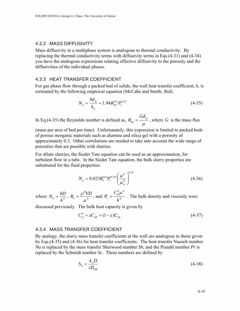
4.3.3 HEAT TRANSFER COEFFICIENT For gas phase flow through a packed bed of solids, the wall heat transfer coefficient, h, is estimated by the following empirical equation (McCabe and Smith, ibid).
33.05.094.1 repg
pu PR
khd
N == (4-35)
In Eq.(4-35) the Reynolds number is defined as, µ
pep
GdR = , where is the mass flux
(mass per area of bed per time). Unfortunately, this expression is limited to packed beds of porous inorganic materials such as alumina and silica gel with a porosity of approximately 0.3. Other correlations are needed to take into account the wide range of porosities that are possible with slurries.
G
For dilute slurries, the Sieder Tate equation can be used as an approximation, for turbulent flow in a tube. In the Sieder Tate equation, the bulk slurry properties are substituted for the fluid properties:
14.0
0
0333.08.0023.0 ⎟⎟
⎠
⎞⎜⎜⎝
⎛=
wreu PRN
µµ (4-36)
where 0khDNu = , 0
0
µρ VDRe = , and 0
00
kC
P pr
µ= . The bulk density and viscosity were
discussed previously. The bulk heat capacity is given by
(4-37) pspfp CCC )1(0 εε −+=
4.3.4 MASS TRANSFER COEFFICIENT By analogy, the slurry mass transfer coefficients at the wall are analogous to those given by Eqs.(4-35) and (4-36) for heat transfer coefficients. The heat transfer Nusselt number Nu is replaced by the mass transfer Sherwood number Sh, and the Prandtl number Pr is replaced by the Schmidt number Sc. These numbers are defined by
AB
xh c
DkS
D= (4-38)
4-19

SOLIDS NOTES 4, George G. Chase, The University of Akron
AB
cSDρµ
= (4-39)
4.3.5 DISPERSIVITY (FLOW EFFECTS) Numerous correlations are available in references and textbooks. For example, in McCabe and Smith (ibid) for a porous inorganic material such as alumina, silica gel, or an impregnated catalyst, the effective thermal conductivity of the bed is proportional to the gas phase thermal conductivity, kg, given by
repg
PRkk 1.05
0
+≈ (4-40)
This shows that the effective thermal conductivity is affected by the flow rate, due to a dispersion mechanism. Dispersion is caused by the fluid following tortuous paths and becoming intermixed in the lateral directions normal to the prevailing direction of flow.
4.4 Hindered Settling What happens when particles settle in concentrated solutions?
As each particles falls it displaces fluid which in turn must move upward. In a concentrated system this causes an upward fluid motion which interferes with the motion of other particles. This is shown in Figure 4-13.
DISPLACED FLUID
FALLINGPARTICLES
Figure 4-13. Hindered settling: as a particle falls its displaced fluid moves upward and
slows the observed settling rate of neighboring particles.
4-20

SOLIDS NOTES 4, George G. Chase, The University of Akron
The net effect is a slower, hindered, settling rate for the group of particles as compared to the free settling terminal velocity of one particle by itself.
Coe and Clevenger (Trans. Am. Inst. Min. Met. Eng. 55, 356, 1916) observed that during a batch settling operation, the sedimenting fluids develop several “zones” (Figure 4-14). In zone A the particles are in low concentration and settle at their terminal velocity. In zones B and C the particles are in hindered settling. In zone D the sediment has particles in contact with each other; the particles are no longer settling though the sediment may compact due to the weight of the overburden. The concentration of the particles in zone D near the C - D interface is approximately that of “loose packing” as given by the correlation in Figure 4-5. Not all four zones are present in all settling processes.
Zone A = clear liquid zone.Zone B = constant composition zone.Zone C = variable composition zone.Zone D = sediment.
C
D
B
A
Figure 4-14. Zones of settling observed by Coe & Clevenger.
T. Allen (Particle Size Measurement, Volume 1, 5th ed, Chapman & Hall, London, 1997, page 224) notes that zone B settles in mass and the relative motion of fluid to particles is analogous to flow through a packed bed, hence Eq. (4-25) could be used here to model the motion of zone B.
Maude & Whitmore (Br. J. Appl. Phy. 9, 477-482, 1958) modeled the hindered settling process as a power law in the concentration (volume fraction of the liquid phase)
(4-41) u us tn= ε
where for dilute solutions ε →1 and . Here is calculated as in Chapter 3 for a single particle falling through a clear fluid and accounts for the hindered settling effects. The parameter n is determined experimentally. Unfortunately n is not a constant but varies as a function of the particle geometry and the Reynolds number. Perry’s Handbook (6
us → ut tunε
th ed, pg 5-68) shows that n varies from 2.3 to 4.5 for spherical particles and has a dramatic effect on the calculated values for the hindered settling velocity.
4-21

SOLIDS NOTES 4, George G. Chase, The University of Akron
In the section that follows a rational approach to hindered settling is described in which the particle settles through the slurry instead of the clear fluid. This approach is a preferred alternative to the Maude & Whitmore approach.
4.4.1 RATIONAL ANALYSIS OF HINDERED SETTLING The primary reasons for the phenomena of hindered settling are:
(a) Large particles fall at a different rate relative to a suspension of smaller particles so that the effective density and viscosity of the fluid are increased,
(b) In high concentrations, larger volumes of fluid are displaced causing an upward fluid velocity. The settling velocity to an external observer is different than the effective velocity difference be the two phases, and
(c) Velocity gradients in the fluid near the particle surfaces are increased as a result of the concentration of the particles.
Terminal velocity of a single particle is correlated through the drag coefficient as given by the defining equation relating the kinetic force acting on the particle and the particle’s kinetic energy,
CD
F C A KE
Cd
u
k d
Dp
t
=
=⎛
⎝⎜⎜
⎞
⎠⎟⎟⎛⎝⎜
⎞⎠⎟
πρ
22
412
(4-42)
where is the observed velocity of the particle relative to the stationary vessel walls. actually represents the velocity difference between the particle and the stationary fluid phase,
ut ut
u v . (4-43) vts= − f
When settling occurs in a large vessel of cross-sectional area A the displaced fluid velocity is negligible. Let the z-direction be the direction of gravity; then the particles have a positive velocity in the z-direction and the fluid has a negative velocity opposite to the direction of gravity. At steady state the volume rate of flow of particles downward must equal the volume rate of flow of fluid upward. We can write this as
πd
v Avp s2
4⎛
⎝⎜⎜
⎞
⎠⎟⎟ = − f (4-44)
where A is large and hence v f is small compared to . v s
In hindered settling the volume rate of flow of particles is related to the fluid phase velocity through the solid phase volume fraction ( )1− ε and the vessel cross sectional area, A, by
( ) (4-45) fs AvAv εε −=−1
or
4-22

SOLIDS NOTES 4, George G. Chase, The University of Akron
( )
v f = −−1 ε
v s
ε. (4-46)
Since the terminal velocity is the relative velocity difference between the solid particle downward motion and the fluid phase upward motion, then
( )
u v v
v
v
ts f
s
s
= −
= +−
=
1 εε
ε
v s
u
(4-47)
and the velocity observed by an external observer is
. (4-48) v st= ε
This is consistent with the extreme case of dilute solutions. In the limit when only one particle is present, ε →1, the observed velocity approaches the terminal velocity,
. v ust→
For more concentrated solutions the particles interfere with the drag coefficients on each other. Davis and Hill (J. Fluid. Mech, 236, 513-533, 1992) studied hindered settling with spheres falling through slurries of neutrally buoyant particles. Their work assumes Brownian motion and interparticle attractive/repulsive forces are negligible. The results of their work show the velocity effects are nearly independent of particle size ratio.
Geankoplis (Transport Processes and Unit Operations, 3ed, Prentice Hall, Englewood Cliffs, 1993, pg 820) suggests that we replace the fluid phase density and viscosity, ρ and µ in the hindered settling correlations with the slurry bulk density and bulk viscosity, ρo and µo , where
( ) pρερερ −+= 10 (4-49)
and (4-50) ( )εµµ f=0
where ( )εf is a function of the fluid phase volume fraction, ε , as related through Eqs.(4-3) to (4-9). Effectively we are saying that the fall of a single particle in a slurry is the same as if all of the other particles in the slurry are part of the surrounding fluid phase.
For neutrally buoyant particles in the slurry (but the falling particle is not neutrally buoyant), in the Stoke’s Law range the observed velocity is given by the modifying Stoke’s Law, Eq.(3-61) to be
( )
0
02
18µρρ −
== ppot
s dguv . (4-51)
If all of the particles in the surrounding slurry are also setting, then we must take into account the upward motion of the fluid phase as done in Eq.(4-40) which gives
4-23

SOLIDS NOTES 4, George G. Chase, The University of Akron
( )
0
02
18µρρε
ε−
== ppot
s dguv . (4-52)
This assumes all of the particles are approximately the same size and density.
How can we approach this problem if the particles have a variation in size and density? If there is a variation in the size or density of the particles, then the different types of particles will settle at different rates.
Let be the observed velocity of the ivis th type of particles (of size and density d pi ρi )
which occupy a solid phase volume fraction (volume of all iε is th particles divided by
total volume).
The bulk density becomes
∑+= isi ρερερ 0 (4-53)
where is the total volume fraction occupied by the solid phase. We have no additional information on the bulk viscosity so we use the same models as given in Eqs.(4-3) through (4-9).
(ε ε εis s∑ = = −1 )
s
f
Since the velocities are different, we must relate all of the velocities to the volumetric rate of displacement,
(4-54) Q A v
A v
s s s
is
is
== ∑
εε
The fluid phase displacement is given by
Q A (4-55) v Qf f= = −ε
We are not interested in a mass average solid phase velocity. The drag coefficient correlation reflects the fact that we are accelerating the fluid around the particle, hence we are actually interested in the volumetric flow rate so we can relate it to the fluid phase mass.
The terminal velocity of the ith size particle is
u v (4-56) vti is= −
which can be manipulated as
4-24
SOLIDS NOTES 4, George G. Chase, The University of Akron
u vQA
vA vA
vv
ti is
s
is i
sis
is i
s js
js
j i
= +
= +
= +⎛
⎝⎜
⎞
⎠⎟ +
∑
∑≠
εεε
εε
ε
ε1
(4-57)
or upon rearrangement, we get the expression
( )vu v
is
ti js
js
j i
is=−
+≠∑ε ε
ε ε (4-58)
which is the expression that applies to settling Zone C. In estimating values for in Eq.(4-58) one may use the modified forms (substitute bulk density and bulk viscosity for the fluid properties) of Stoke’s Law, Newton’s Law or intermediate range, depending upon the Reynold’s number for the particle size.
uti
Since Eq.(4-50) is the most general form we can apply it to several example cases to demonstrate its utility.
4.4.2 CASE STUDY COMPARISONS IN HINDERED SETTLING
CASE 1: One particle in free settling.
This is the simplest case. Since there is only one particle, there is only one particle size. The fluid occupies a significantly greater volume hence ε =1 and , the fluid density is the same as the bulk density, , and the fluid viscosity is the same as the bulk viscosity, . Equation (4-58) reduces to
ε1 0s =0ρρ =
0µµ =
( ) 11
1 100)1(
tts u
uv =
+−
= (4-59)
where the summation term is zero because no terms exist for ε js
js
j iv
≠∑ j ≠ 1. Hence
Eq.(4-58) reduces to the solids velocity equals the terminal velocity, as expected.
CASE 2: One particle settling in a slurry of neutrally buoyant particles.
In this case, the neutrally buoyant particles affect the bulk viscosity of the slurry, but not the bulk density. The neutrally buoyant particles are of a concentration represented by volume fraction which is non zero. The settling particle, as in Case 1, has a volume fraction of essentially zero, .
ε2 0s ≠ε1 0s →
4-25

SOLIDS NOTES 4, George G. Chase, The University of Akron
Since all of the volume fractions must sum to 1, we get ( )ε ε= −1 2s . Equation (4-58)
gives the estimated velocities to be
( )
v u us ts
t11 2
10
0=
−+
=ε ε
ε (4-60)
Where the velocity of the neutrally buoyant particles is zero because the remain motionless with the fluid phase. This tells us that the particle settles at its modified terminal velocity rate where ( )00
11 ,µρtt uu = . As a consistency check, Eq.(4-58) gives the velocity of the neutrally buoyant particles to be zero, . v s
2 0=
CASE 3: Group of particles of same size all settling at the same rate.
This case is more complex than Case 2 because now there are many particles settling, not just one particle. There are no neutrally buoyant particles present in this system. The volume fraction, occupied by the particles is not zero. This results in 1 . ε1
s1= +ε ε s
Since only one type of particle is present in the system, the summation term in the numerator of Eq.(4-50) summed over j i≠ is identically zero. The observed velocity becomes
(4-61) where the terminal velocity is a function of the bulk density and viscosity.
v ust1 = ε 1
CASE 4: Two sizes of particles settling at different velocities.
This is the most complex case that will be considered here. In this case there are two particle sizes, denoted 1 and 2. Neither of the particles are neutrally buoyant. The volume fractions are related by
1 . (4-62) 1= + +ε ε εs2s
The observed velocities are determined from Eq.(4-58) to be
( )s
ssts vuv
2
2211 1 ε
εε−−
= (4-63)
and ( )s
ssts vuv
1
1122 1 ε
εε−−
= (4-64)
where we see that the two velocities are interdependent. If we use Eq.(4-64) to eliminate the velocity of particle 2 from the right side of Eq.(4-63) then we get the velocity of particle 1 as a function of the terminal velocities of both particles,
. (4-65) ( )v us st
st1 1 1 21= − −ε ε u 2
4-26

SOLIDS NOTES 4, George G. Chase, The University of Akron
With Eq.(4-65) we can calculate the observed settling velocities for the two types of particles present in the slurry.
The limitations of the results are reiterated here for emphasis. These results assume laminar, slow flow conditions. If there are any disturbances in the slurry then the eddy currents will disrupt the flow patterns. Also, these results only hold as long as the volume fractions are constant. The settling process is inherently unsteady hence these results only hold at the moment in time that the concentrations are those used in the equations; the concentrations will vary with time and position.
Sedimentation of multicomponent mixtures has been the subject of numerous papers in literature. See for example: J. F. Richardson, and R.A. Meikle, “Sedimentation and Fluidization Part III, The Sedimentation of Uniform Fine Particles and of Two-Component Mixtures of Solids,” Trans. Inst Chem. Engr, 39, 348-356, 1961.
EXAMPLE 4-3. Calculate the observed settling velocities of a mixture of latex spheres and sand in water.
Suppose a mixture of latex spheres (39 microns, intrinsic density of 1.18 g/cm3) and sand (1 mm, intrinsic density of 2.5 g/cm3) are settling in water at room temperature. Estimate the observed velocities of the latex and the sand.
The mixture is uniformly mixed (initially) with and as the volume fractions occupied by each type of particle. The water volume fraction is given by . The water viscosity is 1.0 cP and using Eq.(4.4) the slurry bulk viscosity is estimated to be 1.409 cP. With the water density of 1000 kg/m
ε latexs = 01. εsand
s = 0 05.
ε ε ε= − − =1 latexs
sands .085
3, the bulk density is calculated using Eq.(4-2) to be 1093 kg/m3.
Assuming Stoke’s law range, the terminal velocity of the latex particles is calculated to be 4.394x10⁻⁵ m/s using Eq.(3-61) modified with the bulk density and viscosity
( )
0
02
18µρρ −
= latexlatexlatex
gdu . (4-66)
The Stoke’s Law assumption is checked by the Reynold’s number which calculates to be 0.0013 using
0
0
µρ latexlatex
e
duR = . (4-67)
Similarly, the terminal velocity for the sand is estimated from Stoke’s Law to be 0.462 m/s but the Reynold’s number is 421 which places the sand in the intermediate range. A check of Newton’s Law range, given by Eq.(3-62) modified with the bulk density and viscosity gives a terminal velocity of 0.1649 m/s and Reynold’s number of 150, also indicates the intermediate range. Hence, the intermediate range Eq.(3-60) must be used, which is modified as
4-27

SOLIDS NOTES 4, George G. Chase, The University of Akron
⎟⎟⎠
⎞⎜⎜⎝
⎛ −= 0
0
34
ρρρ sand
D
sandsand C
gdu (4-68)
with the drag coefficient given by
(4-69) CD = 185 3 5. / /Rep
from Figure 3-12.
Since the terminal velocity in Eq.(4-68) depends upon itself, through the Reynold’s number, then an iterative solution is needed. Using successive substitution a guess for the terminal velocity is used to calculate the Reynold’s number, calculate the drag coefficient, and calculate a new guess for the velocity. This set of calculations is easily computed using a computer spreadsheet.
guess u Re Cd calc u0.35 271.5046 0.64107 0.16204
0.16204 125.6987 1.017591 0.1286140.128614 99.76932 1.16889 0.1200020.120002 93.08867 1.218523 0.1175320.117532 91.17311 1.23382 0.1168020.116802 90.60617 1.238446 0.1165830.116583 90.43677 1.239837 0.1165180.116518 90.38602 1.240255 0.1164980.116498 90.37079 1.24038 0.1164920.116492 90.36623 1.240418 0.116490.11649 90.36486 1.240429 0.11649
Hence the terminal velocity of the sand is =sandu 0.11649 m/s.
Using Eq.(4-57) the observable velocities of the latex and the sand are m/s and m/s. The negative value for the
observed latex velocity indicates that the velocity is upward! vsand
s = 011066. vlatexs = −0 00578.
The observable velocity of the water may be determined from Eq.(4-58) with some manipulation as
vvf i
sis
= −
= −
∑εε
0 00617. m / s (4.70)
for which the minus sign indicates upward flow. Flotats (Hungarian J. Indust. Chem, 23, 215, 1995) argues that in sedimentation the smallest particles may move upward with this fluid motion as indicated by the negative fluid and latex velocities.
4-28

SOLIDS NOTES 4, George G. Chase, The University of Akron
4.5 Slurry Flows Cheremisinoff’s book (N.P. Cheremisinoff and R. Gupta, Handbook of Fluids in Motion, M.C. Roco ed., Ann Arbor Science, Ann Arbor, Michigan, 1983) and the Encyclopedia of Fluid Mechanics are two examples of good references that discuss slurry flows. Many concentrated suspension display non-Newtonian flow behavior, even when the suspensions are spherical. Therefore the bulk viscosity correlations described previously in Section 4.2 must be used with some caution.
Some slurries can be influenced by electrical and magnetic forces that change their flow behavior. Electrorheological fluids (H. Conrad, “Structure and Mechanisms of Electro-Rheological (ER) Fluids,”Chapter 12, in Particulate Two-Phase Flow, Butterworth, Boston, 1993) are fluids that change properties under the influence of electrical fields. With no electrical field the fluid flows like a Newtonian; with the electrical field the fluid flows like a yield-stress fluid.
The ER fluid is made up of a non-conducting liquid phase and a conducting or semiconducting particulate phase. The mechanism by which this works is due to the particles lining up when an electrical field is applied. This is shown in Figure 4-15. This is one example of how slurry behavior is not a simple extension of the carrier fluid’s properties.
Figure 4-15. Alumina particles in a silicone oil line up in fibers when an electrical field of 1000 volts per centimeter is applied.
Another way that slurry behavior differs from the carrier fluid is when phase separation occurs. This is especially true for gas-liquid systems. Kao (D.T.Y. Kao, “Rheology of
4-29

SOLIDS NOTES 4, George G. Chase, The University of Akron
Suspensions,” Chapter 33, in Handbook of Fluids in Motion, N.P. Cheremisinoff and R. Gupta eds., Ann Arbor Science, Ann Arbor, Michigan, 1983) classifies suspension flow behavior as:
Single Phase Homogeneous
Fine Dispersions Pseudo-Homogeneous
Coarse Dispersions Heterogeneous
Macro-mixed Heterogeneous
Stratified Heterogeneous
A single phase by definition is homogeneous, because its material content does not vary with position. Fine dispersions are termed pseudo homogeneous because even though two phases are present, at a local scale the two phases are well among each other. Coarse dispersions are typically those with large particles (relative to the size of the slurry pipeline) and the larger particles may have a tendency to settle quickly. Macro-mixed dispersions have regions of high concentration of particles and regions of low concentrations of particles, and these regions are located somewhat randomly throughout the slurry. Stratified flows have regions of high concentrations of particles in a layer located at the bottom of a pipe, for example, and low concentration at the top of the pipe.
4-30

SOLIDS NOTES 4, George G. Chase, The University of Akron
4. BULK PROPERTIES OF POWDERS AND SLURRIES In the process industries economics usually requires us to handle and process many particles at a time rather than individually. Because of this we must have a working knowledge of the collective or “bulk” properties of these materials.
The “collective” properties are the measurable properties of groups of particles. Some of these properties are analogous to properties that are measured on individual particles while other properties may not be defined for individual properties.
Some important examples are discussed here, but the list is not complete.
4.1 Brief Overview of Some Bulk Properties
4.1.1 ANGLE OF REPOSE The angle of repose is a characteristic of solids which characterizes the piling or stacking nature of the particles. The way that particles stack when poured into a pile is a function of the size/shape, particle intrinsic density, surface forces (stickiness, electrostatic), and roughness of the particles. Many factors can influence the way particles stack hence it is difficult to predict; normally a simple measurement can be made to determine the angle of repose.
F
Ththecorgivlonto Thdet
b.
α
a.
α α
c.
igure 4-1. Angle of repose, α, of (a) a pile of powder, (b) powder in a container, and (c) powder in a rolling drum.
e angle of repose is considered to be mostly a measure of the internal friction between particles as a whole, but not between individual particles. It is used in a number of relations and estimates for the behavior properties of the bulk solids. One example en in Coulson and Richardson’s text relates the angle of repose to the height of the gest movable plug in a piston. The angle of repose may is often incorrectly be used
estimate the angle required for the bottom of a hopper to ensure proper discharge. ere are more appropriate methods for designing hoppers which will be discussed in ail later.
4-1

SOLIDS NOTES 4, George G. Chase, The University of Akron
The best use of the angle of repose is to determine the size of a pile of powder or granular materials, either volume or ground area that such a pile will occupy. Figures 4-2 and 4-3 show typical piles of such materials.
Figure 4-2.
Figure 4-3. mountain is
Large gravel piles at rock and stone facility near Marblehead, Ohio.
Baldy Mountain, Philmont Boy Scout Ranch, New Mexico. The top of the largely loose rock and stone that prevent plants from taking root.
4-2

SOLIDS NOTES 4, George G. Chase, The University of Akron
4.1.2 POROSITY (VOLUME FRACTION) Porosity is the fraction of volume space that is NOT occupied by the solid particles.
If you have a two phase system of solids and liquid, you can add the respective volumes to obtain the total volume of your mixed system.
=+
VMIXTURVLIQUUIDVSOLIDS
Figure 4-4. Addition of phase volumes yields the total volume.
The porosity is defined as the volume fraction of the fluid phase:
ε =V
VLIQUID
MIXTURE (4-1)
Since porosity is defined as a fraction it must have a value between 0 and 1 inclusive. ε is the fluid phase volume fraction. (1-ε) is the solid phase volume fraction. Their sum is 1.
Handout 12 (Appendix B of Foust et.al., Principles of Unit Operations, Wiley, NY, 1960) provides correlations for estimating porosity of packed beds as a function of sphericity.
4.1.3 BULK DENSITY Bulk density is the effective density of a powder or particulate solid taking into account the volume occupied by both the solid and fluid phases. The bulk density is calculated from the porosity and the intrinsic densities of the fluid and solid phases:
( ) po ρερερ −+= 1 . (4-2)
EXAMPLE 4-1. An example of applying bulk density is determining the weight of sand in a bucket. The intrinsic density of one sand particle is about the same as that of glass, 2.6 g/cm3. If sand packs with a porosity of 0.4, how much will a twenty five liter bucket filled level to the top with dry sand weigh?
The mass of sand in the bucket is given by
BUCKEToVMass ρ=
Applying Eq.(4-2), neglecting mass of the air (air density is about 1/2600 that of the sand), we get
33 /1560/2600)4.01( mkgmkgo =−=ρ
4-3
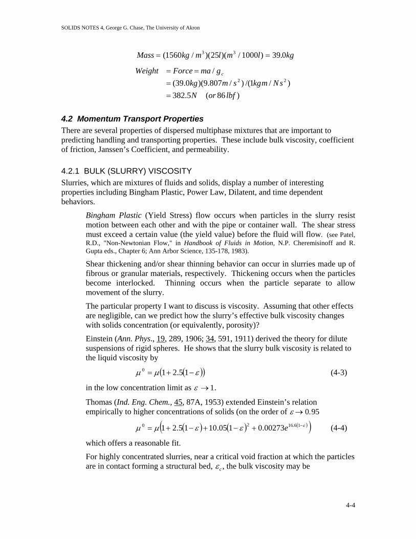
SOLIDS NOTES 4, George G. Chase, The University of Akron
Mass kg m l m l kg= =( / )( )( / ) .1560 25 1000 39 03 3
)86(5.382
)/1/()/807.9)(0.39(/
22
lbforNsNmkgsmkg
gmaForceWeight c
==
==
4.2 Momentum Transport Properties There are several properties of dispersed multiphase mixtures that are important to predicting handling and transporting properties. These include bulk viscosity, coefficient of friction, Janssen’s Coefficient, and permeability.
4.2.1 BULK (SLURRY) VISCOSITY Slurries, which are mixtures of fluids and solids, display a number of interesting properties including Bingham Plastic, Power Law, Dilatent, and time dependent behaviors.
Bingham Plastic (Yield Stress) flow occurs when particles in the slurry resist motion between each other and with the pipe or container wall. The shear stress must exceed a certain value (the yield value) before the fluid will flow. (see Patel, R.D., "Non-Newtonian Flow," in Handbook of Fluids in Motion, N.P. Cheremisinoff and R. Gupta eds., Chapter 6; Ann Arbor Science, 135-178, 1983).
Shear thickening and/or shear thinning behavior can occur in slurries made up of fibrous or granular materials, respectively. Thickening occurs when the particles become interlocked. Thinning occurs when the particle separate to allow movement of the slurry.
The particular property I want to discuss is viscosity. Assuming that other effects are negligible, can we predict how the slurry’s effective bulk viscosity changes with solids concentration (or equivalently, porosity)?
Einstein (Ann. Phys., 19, 289, 1906; 34, 591, 1911) derived the theory for dilute suspensions of rigid spheres. He shows that the slurry bulk viscosity is related to the liquid viscosity by
( )( εµµ −+= 15.210 ) (4-3)
in the low concentration limit as ε → 1.
Thomas (Ind. Eng. Chem., 45, 87A, 1953) extended Einstein’s relation empirically to higher concentrations of solids (on the order of ε → 0 95.
( ) ( ) ( )( )εεεµµ −+−+−+= 16.1620 00273.0105.1015.21 e (4-4)
which offers a reasonable fit.
For highly concentrated slurries, near a critical void fraction at which the particles are in contact forming a structural bed, εc , the bulk viscosity may be
4-4

SOLIDS NOTES 4, George G. Chase, The University of Akron
approximated by (Art Etchels, personal communication, DuPont, Delaware, 1994)
( )( )
5.20
111
−
⎟⎟⎠
⎞⎜⎜⎝
⎛−−
−=cεεµµ (4-5)
which says that the closer the porosity gets to the critical porosity ε ε→ c the more the slurry behaves like a solid structure. Another correlation is Shook Eq. listed in homework problem E3.
To estimate the values of cε one can use the porosity of a loosely packed bed. Foust, Appendix B, gives a correlation between sphericity and porosity and Loose, Normal, and Dense packing (A.S. Foust, L.A. Wenzel, C.W. Clump, L. Maus, and L.B. Andersen, Principles of Unit Operations, Wiley, New York, 1960). The data taken from Foust’s figure is plotted in Figure 4-5 in a slightly different format. (Handout 4.1)
FpaADamfo
1
The plot infunction o
All three c
igure 4-5. Porosity as a function of sphericity and packing structure. Loose cked materials are ones that have not had much time to settle due to vibrations. normal packed material is one that may have sat for several days or weeks. ense packed materials are ones that have sat for a year or more and have had ple time to settle and vibrate into its most densely packed structure under
rce of gravity.
00.10.20.30.40.50.60.70.80.9
0 0.1 0.2 0.3 0.4 0.5 0.6 0.7 0.8 0.9 1
Sphericity
Poro
sity
LooseNormalDense
Figure 4-5 is obtained by curve fitting data. The loose packed porosity is a f sphericity given by
(4-6) 0873.11042.14411.0 2 +Φ−Φ=Looseε
urves are generated by defining a packing parameter, λ , such that
4-5

SOLIDS NOTES 4, George G. Chase, The University of Akron
(4-7) ⎪⎩
⎪⎨
⎧=
Packing Densefor 1Packing Normalfor 5.0
Packing Loosefor 0λ
and the porosity is given by
( )( Loose)ελε 08.0297.01 −Φ−= (4-8)
for any packing condition.
Etchel’s equation, Eq.(4-5) is a special case of the Krieger-Dougherty Equation (I.M. Krieger and T.J. Dougherty, Trans.Soc. Rheol., 3, 137-152, 1959) which has the form
( )( )
)1(0
111
cA
c
ε
εεµµ
−−
⎟⎟⎠
⎞⎜⎜⎝
⎛−−
−= (4-9)
where A is a material parameter. Bird et.al. (R.B. Bird, W.E. Stewart, and E.N. Lightfoot, Transport Phenomena, 2nd ed., Wiley, New York, 2002) list values for parameter A from several references.
A plot of the data in Figure 4-6 gives a rough approximation between A and εc as
cA ε1.10≅ (4-10)
The data points in the plot are scattered meaning that Eq.(4-6) should only be used if experimental data are not available. (Handout 4.2)
y = 10.107xR2 = 0.4134
0
2
4
6
8
10
12
0 0.1 0.2 0.3 0.4 0.5 0.6 0.7 0.8 0.9
A
εc
Material A cε
Submicron spheres 2.7 0.29 40 micron spheres 3.28 0.39 Ground Gypsum 3.25 0.31 TiO2 5.0 0.45 Laterite 9.0 0.65 Glass Rods 30x700µm 9.25 0.732 Glass Rods 100x400µm 9.87 .618 Quartz grains 53-76 µm 5.8 .629 Glass fiber aspect ratio 7 3.8 0.626 Glass fiber aspect ratio 14 5.03 0.74 Glass fiber aspect ratio 21 6.0 0.767
Figure 4-6 Relation between parameter A and εc in Eq. (4-10).
4-6
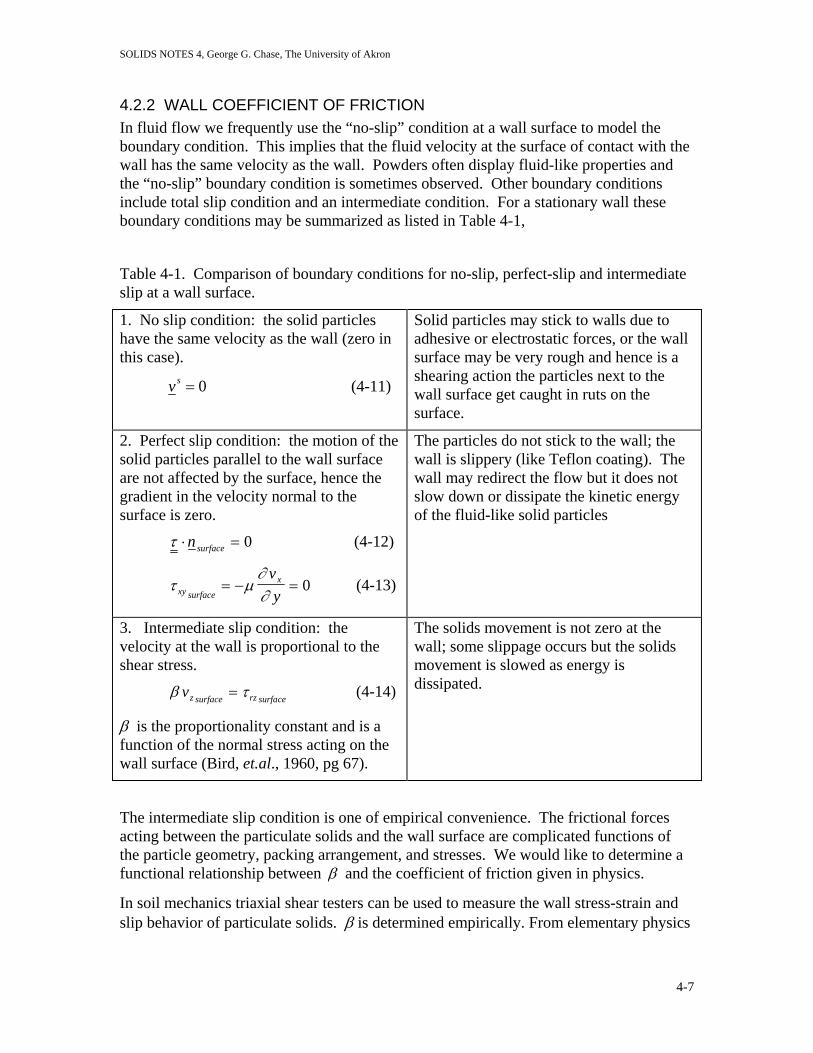
SOLIDS NOTES 4, George G. Chase, The University of Akron
4.2.2 WALL COEFFICIENT OF FRICTION In fluid flow we frequently use the “no-slip” condition at a wall surface to model the boundary condition. This implies that the fluid velocity at the surface of contact with the wall has the same velocity as the wall. Powders often display fluid-like properties and the “no-slip” boundary condition is sometimes observed. Other boundary conditions include total slip condition and an intermediate condition. For a stationary wall these boundary conditions may be summarized as listed in Table 4-1,
Table 4-1. Comparison of boundary conditions for no-slip, perfect-slip and intermediate slip at a wall surface.
1. No slip condition: the solid particles have the same velocity as the wall (zero in this case).
vs = 0 (4-11)
Solid particles may stick to walls due to adhesive or electrostatic forces, or the wall surface may be very rough and hence is a shearing action the particles next to the wall surface get caught in ruts on the surface.
2. Perfect slip condition: the motion of the solid particles parallel to the wall surface are not affected by the surface, hence the gradient in the velocity normal to the surface is zero.
τ ⋅ =nsurface 0 (4-12)
τ µ∂∂xy surface
xvy
= − = 0 (4-13)
The particles do not stick to the wall; the wall is slippery (like Teflon coating). The wall may redirect the flow but it does not slow down or dissipate the kinetic energy of the fluid-like solid particles
3. Intermediate slip condition: the velocity at the wall is proportional to the shear stress.
β τvz surface rz surface= (4-14)
β is the proportionality constant and is a function of the normal stress acting on the wall surface (Bird, et.al., 1960, pg 67).
The solids movement is not zero at the wall; some slippage occurs but the solids movement is slowed as energy is dissipated.
The intermediate slip condition is one of empirical convenience. The frictional forces acting between the particulate solids and the wall surface are complicated functions of the particle geometry, packing arrangement, and stresses. We would like to determine a functional relationship between β and the coefficient of friction given in physics.
In soil mechanics triaxial shear testers can be used to measure the wall stress-strain and slip behavior of particulate solids. β is determined empirically. From elementary physics
4-7
SOLIDS NOTES 4, George G. Chase, The University of Akron
we know that frictional forces oppose movement (Haliday & Resnick, Fundamentals of Physics, Wiley, NY, 1974, pg 78).
Two surfaces that are in contact may appear to be smooth, but at a sufficient small scale the surfaces are rough and jagged. The interlocking of the jagged edges between the surfaces causes the friction. Also, there may be attractive forces (static charge, etc.) that resist motion.
An initial force is required to overcome the resistances due to the interlocked jagged edges and to cause separation between the surfaces so that they may move relative to each other. Once in motion the force required to keep them in motion is less than the initial force. The final force to keep the surfaces in relative motion increases with increasing velocity.
If you recall the drag coefficient Stokes’ Law for a sphere, Eqs. 3-58, 3-59, and 3-42, we deduce that in Stoke’s law range the drag force is proportional to the velocity. Hence by analogy we should not be surprised to find the coefficient of friction to be a function of velocity (though for powdered materials it may be a weak function of velocity).
4-8

SOLIDS NOTES 4, George G. Chase, The University of Akron
Consider a block of mass M resting on a horizontal surface (Figure 4-7a). When we apply a force parallel to the surface the block does not move until the applied force exceeds the maximum static frictional force (Figure (4-7b,c).
Once the motion starts the force F required to maintain motion usually decreases, which means that the kinetic frictional force is less than the maximum static frictional force,
. (4-15) f s(max) > f k
N
If force F is held constant, the block will accelerate due to the imbalance between the forces until the kinetic frictional force increases to balance F (Figure 4-7d).
The static and kinetic forces are functions of the normal force, N, holding the block against the surface.
Normally we model the relationship between the forces as
f s s≤ µ (4-16)
f k k= Nµ (4-17)
where µs and µk are the coefficients of static and kinetic friction. Also, the kinetic friction varies with velocity (otherwise the kinetic friction could never balance the applied force as shown in Figure 4-7d). We assume a linear dependence by letting µ µk k= ' to obtain
f k k= vNµ ' . (4-18)
At steady state we get
F vk= Nµ ' . (4-19)
N= -Mg
gBLOCK
SURFACE
(a) Block of mass M on surface.
N= -Mg
g
F fs
(b) Force F is balance by the static friction fs.
g
F
N= -Mg
fs(max)
(c) No motion occurs until F exceeds fs(max).
Motion, dv/dt > 0g
F
N= -Mg
fk
(d) As long as force F exceeds the kinetic friction, fk, the block accelerates. Acceleration stops when F is again
balanced by the frictional force, fk, and the motion becomes steady.
Figure 4-7. Effect of forces acting on a block of mass M resting on a horizontal surface.
4-9
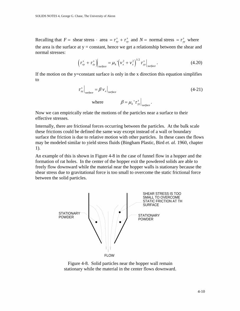
SOLIDS NOTES 4, George G. Chase, The University of Akron
Recalling that and where the area is the surface at y = constant, hence we get a relationship between the shear and normal stresses:
F xys
zys= ⋅ = shear stress area τ τ+ N yy
s= = normal stress τ
( ) ( )τ τ µ τxys
zys
surfacek x z yy
s
surfacev v+ = +'
/2 2 1 2. (4.20)
If the motion on the y=constant surface is only in the x direction this equation simplifies to
τ βxys
surface x surfacev= (4-21)
where β µ τ= k yys
surface' .
Now we can empirically relate the motions of the particles near a surface to their effective stresses.
Internally, there are frictional forces occurring between the particles. At the bulk scale these frictions could be defined the same way except instead of a wall or boundary surface the friction is due to relative motion with other particles. In these cases the flows may be modeled similar to yield stress fluids (Bingham Plastic, Bird et. al. 1960, chapter 1).
An example of this is shown in Figure 4-8 in the case of funnel flow in a hopper and the formation of rat holes. In the center of the hopper exit the powdered solids are able to freely flow downward while the material near the hopper walls is stationary because the shear stress due to gravitational force is too small to overcome the static frictional force between the solid particles.
STATIONARYPOWDER
SHEAR STRESS IS TOOSMALL TO OVERCOMESTATIC FRICTION AT THSURFACE
FLOW
STATIONARYPOWDER
Figure 4-8. Solid particles near the hopper wall remain
stationary while the material in the center flows downward.
4-10
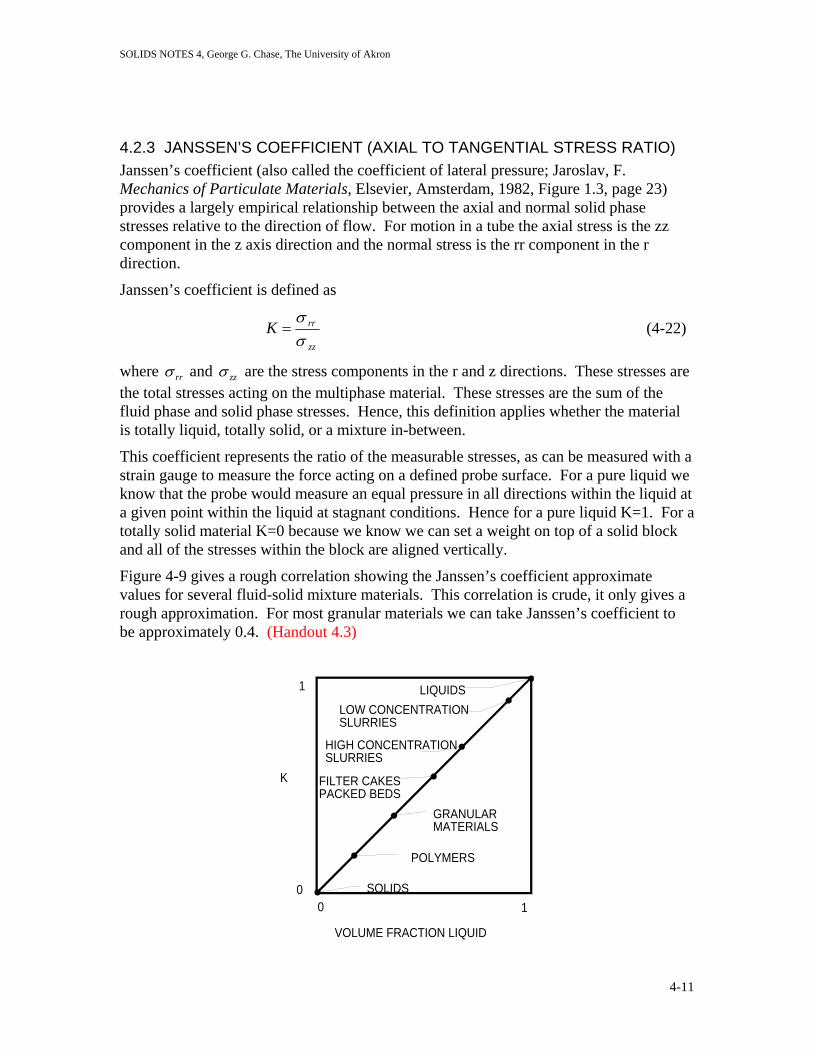
SOLIDS NOTES 4, George G. Chase, The University of Akron
4.2.3 JANSSEN’S COEFFICIENT (AXIAL TO TANGENTIAL STRESS RATIO) Janssen’s coefficient (also called the coefficient of lateral pressure; Jaroslav, F. Mechanics of Particulate Materials, Elsevier, Amsterdam, 1982, Figure 1.3, page 23) provides a largely empirical relationship between the axial and normal solid phase stresses relative to the direction of flow. For motion in a tube the axial stress is the zz component in the z axis direction and the normal stress is the rr component in the r direction.
Janssen’s coefficient is defined as
zz
rrKσσ
= (4-22)
where σ rr and σ zz are the stress components in the r and z directions. These stresses are the total stresses acting on the multiphase material. These stresses are the sum of the fluid phase and solid phase stresses. Hence, this definition applies whether the material is totally liquid, totally solid, or a mixture in-between.
This coefficient represents the ratio of the measurable stresses, as can be measured with a strain gauge to measure the force acting on a defined probe surface. For a pure liquid we know that the probe would measure an equal pressure in all directions within the liquid at a given point within the liquid at stagnant conditions. Hence for a pure liquid K=1. For a totally solid material K=0 because we know we can set a weight on top of a solid block and all of the stresses within the block are aligned vertically.
Figure 4-9 gives a rough correlation showing the Janssen’s coefficient approximate values for several fluid-solid mixture materials. This correlation is crude, it only gives a rough approximation. For most granular materials we can take Janssen’s coefficient to be approximately 0.4. (Handout 4.3)
1
LIQUIDS
FILTER CAKESPACKED BEDS
VOLUME FRACTION LIQUID
SOLIDS00
GRANULARMATERIALS
POLYMERS
LOW CONCENTRATIONSLURRIES
HIGH CONCENTRATIONSLURRIES
K
1
4-11
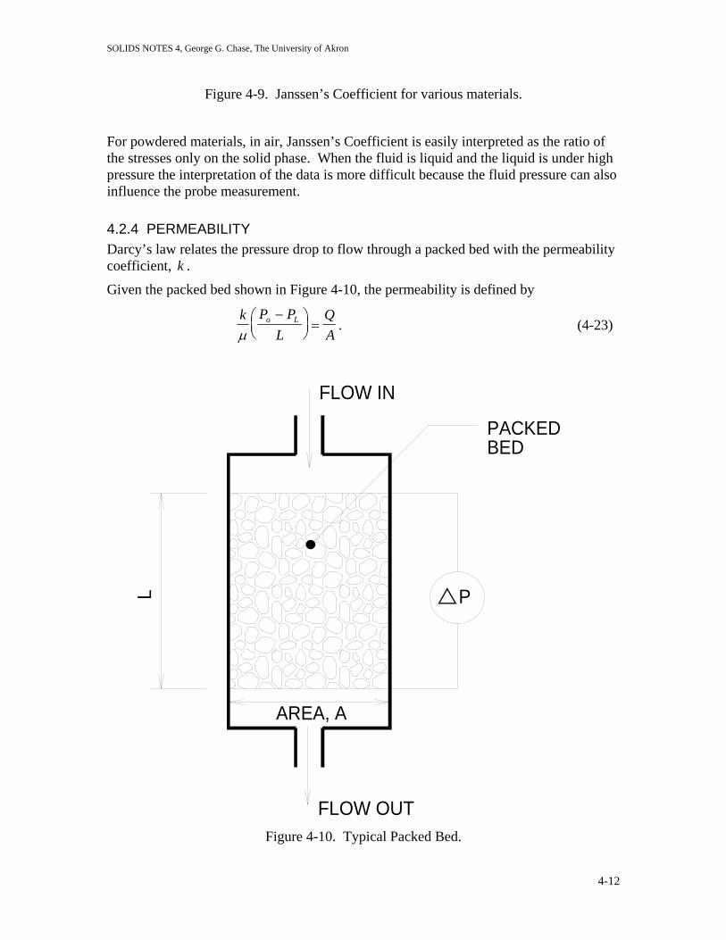
SOLIDS NOTES 4, George G. Chase, The University of Akron
Figure 4-9. Janssen’s Coefficient for various materials.
For powdered materials, in air, Janssen’s Coefficient is easily interpreted as the ratio of the stresses only on the solid phase. When the fluid is liquid and the liquid is under high pressure the interpretation of the data is more difficult because the fluid pressure can also influence the probe measurement.
4.2.4 PERMEABILITY Darcy’s law relates the pressure drop to flow through a packed bed with the permeability coefficient, . k
Given the packed bed shown in Figure 4-10, the permeability is defined by
k P P
LQA
o L
µ−⎛
⎝⎜⎞⎠⎟= . (4-23)
PACKEDBED
L
AREA, A
FLOW OUT
FLOW IN
P
Figure 4-10. Typical Packed Bed.
4-12

SOLIDS NOTES 4, George G. Chase, The University of Akron
Typical permeability values for some common materials are listed in Table 4-2. Also, Coulson & Richardson (Chemical Engineeering, Volume 2, 4th ed, Pergamon, Oxford, 1991, Table 4.1, page 133) has permeability values for common shapes given as B where k=B/µ. The data reported by Coulson & Richardson show that the permeability depends significantly upon porosity and specific surface area of contact between the fluid and solid phases. (Handout 4.4)
Table 4-2. Permeabilities of typical materials.
Material Permeability Coefficient, k (m2)
Clean sand, sand-gravel mixture 10-12 to 10-9
Non-woven glass fiber filter media 10-10 to 10-9
fine sand, silt, loam 10-16 to 10-12
peat 10-13 to 10-11
filter aides (diatomaceous earth, etc.) 10-14 to 10-12
clay 10-16 to 10-13
sandstone 10-16 to 10-11
granite 10-20 to 10-18
The Darcy’s law expression provides a means of estimating the flow rate for a given pressure drop of fluid. The permeability coefficient must be determined from experiment.
A few correlations are available for predicting the permeability. One of the more common correlations is Ergun’s equation (Bird et.al., Transport Phenomena, Wiley, New York, 1960),
( )( ) 75.11150
1
3
2 +Φ
−=
−
Φ∆
µρε
εε
ρopo
pc
VdVd
LPg (4-24)
where
∆P is the pressure drop (pressure at inlet minus pressure at outlet), L is the height (or depth) of the bed, Vo is the approach velocity, flow rate divided by the cross sectional area of
the bedQ
A , and
4-13

SOLIDS NOTES 4, George G. Chase, The University of Akron
gc is the gravity conversion factor 32174.ft lblb s
m
f2 in FPS units or 1
kg mN s2 in
MKS units.
Ergun’s equation relates the pressure drop to a quadratic expression in the superficial velocity (equivalent to ) as a function of the particle size and the bed porosity. One could make a comparison between Darcy’s Law and Ergun’s equation to get a relation for the permeability as a first order function of the superficial velocity.
Q A/
MacDonald et.al. ("Flow Through Porous Media-The Ergun Equation Revisited," Ind. Chem. Fundam., 18(3) 199-207, 1979) studied data on a wider range of particles and concluded that the 150 coefficient in Eq. (4-24) should be replaced with 180 and the 1.75 coefficient should be replaced with 1.80 for smooth particles. For rough particles the 1.75 should be replaced with 4.0.
This gives
( )( ) 80.11180
1
3
2 +Φ
−=
−
Φ∆
µρε
εε
ρopo
pc
VdVd
LPg (4-25)
Lets define the Reynolds number and packed bed friction factor as
( )εµρ
−=
1po
ep
dVR (4-26)
( )εε
ρ −
Φ∆=
1
3
2o
pc
Vd
LPg
f (4-27)
then the Ergun equation can be written as
80.1180+
Φ=
epRf (4-28)
Note that we can deduce a model for permeability from Eq.(4-25). Replace LP∆ in
Eq.(4-25) with c
o
gV
kµ from Eq.(4.23), where AQVo /= and ( ) PPP Lo ∆=− . We get
4-14

SOLIDS NOTES 4, George G. Chase, The University of Akron
( )[ ]ep
p
R
d
kΦ+
−
Φ
=80.1180
1 2
232
ε
ε
(4-29)
This expression is useful for estimating permeability for a powder of a particular size, or estimating particle size from pressure drop – flow rate data.
If the particles are approximately spherical the sphericity is 1.0, and assuming normal packing the porosity is about 0.38 (from Figure 4-5). For small Renolds number the 180 term dominates the denominator. Eq.(4-29) reduces to
(4-30) 24108 pdxk −≅
EXAMPLE 4-2
As an example, very slow flow of water (1 liters/minute per square meter) though a 10 cm thick packed bed of spherical Lucite particles produces a pressure drop of 10kPa. What is the approximate size of the Lucite particles?
SOLUTION:
Solving Darcy’s Law, Eq.(4-23)
cgPL
AQk 1
∆= µ
⎟⎠⎞
⎜⎝⎛⎟⎟⎠
⎞⎜⎜⎝
⎛⎟⎠⎞
⎜⎝⎛⎟⎟⎠
⎞⎜⎜⎝
⎛⎟⎟⎠
⎞⎜⎜⎝
⎛=
−
2
23
2
3
/11
1100001.0
min/60/101min/001.0
mNPa
kgmNs
Pam
smskgx
mm
213107.1 mx −=
Substitute this value for permeability into Eq.(4-30) and solving for dp gives
mxd p51046.1 −=
or the average particle size is about 15 microns.
4-15

SOLIDS NOTES 4, George G. Chase, The University of Akron
Check the Reynolds number, to make sure the low Reynolds number assumption holds:
( )( )( )( )( )( )3.01/101
101560min/min/001.0/10003
63
−= −
−
mskgxmxsmmkgRep
4104 −≅ x
Since Rep is much smaller than 1 then the assumption in deriving Eq.(4-30) holds.
4-16
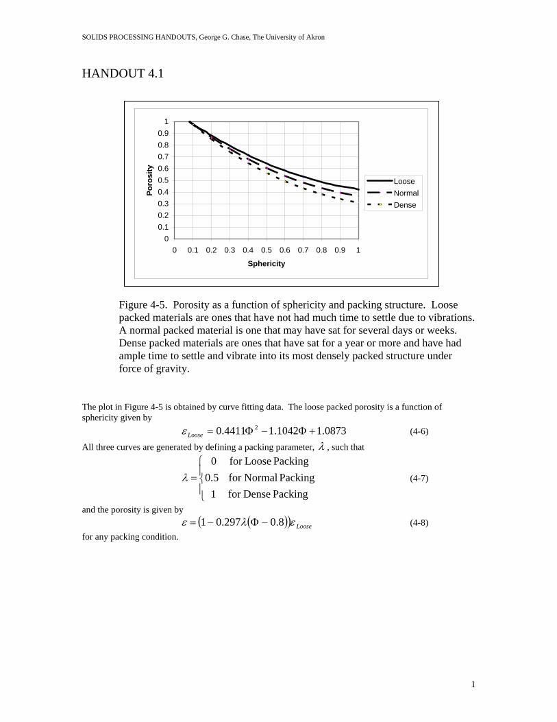
SOLIDS PROCESSING HANDOUTS, George G. Chase, The University of Akron
HANDOUT 4.1
00.10.20.30.40.50.60.70.80.9
1
0 0.1 0.2 0.3 0.4 0.5 0.6 0.7 0.8 0.9 1
Sphericity
Poro
sity
LooseNormalDense
Figure 4-5. Porosity as a function of sphericity and packing structure. Loose packed materials are ones that have not had much time to settle due to vibrations. A normal packed material is one that may have sat for several days or weeks. Dense packed materials are ones that have sat for a year or more and have had ample time to settle and vibrate into its most densely packed structure under force of gravity.
The plot in Figure 4-5 is obtained by curve fitting data. The loose packed porosity is a function of sphericity given by (4-6) 0873.11042.14411.0 2 +Φ−Φ=LooseεAll three curves are generated by defining a packing parameter, λ , such that
(4-7) ⎪⎩
⎪⎨
⎧=
Packing Densefor 1Packing Normalfor 5.0
Packing Loosefor 0λ
and the porosity is given by ( )( Loose)ελε 8.0297.01 −Φ−= (4-8) for any packing condition.
1

SOLIDS PROCESSING HANDOUTS, George G. Chase, The University of Akron
HANDOUT 4.2 Krieger-Dougherty Equation for estimating bulk viscosity of slurries (I.M. Krieger and T.J. Dougherty, Trans.Soc. Rheol., 3, 137-152, 1959) has the form
( )( )
)1(0
111
cA
c
ε
εεµµ
−−
⎟⎟⎠
⎞⎜⎜⎝
⎛−−
−= (4-9)
where A is a material parameter. Bird et.al. (R.B. Bird, W.E. Stewart, and E.N. Lightfoot, Transport Phenomena, 2nd ed., Wiley, New York, 2002) list values for parameter A from several references. A plot of the data in Figure 4-6 gives a rough approximation between A and εc as cA ε1.10≅ (4-10) The data points in the plot are scattered meaning that Eq.(4-6) should only be used if experimental data are not available.
y = 10.107xR2 = 0.4134
0
2
4
6
8
10
12
0 0.1 0.2 0.3 0.4 0.5 0.6 0.7 0.8 0.9
A
♦c
Figure 4-6 Relation between parameter A and εc in Eq
Material A cε
Submicron spheres 2.7 0.29 40 micron spheres 3.28 0.39 Ground Gypsum 3.25 0.31 TiO2 5.0 0.45 Laterite 9.0 0.65 Glass Rods 30x700µm 9.25 0.732 Glass Rods 100x400µm 9.87 .618 Quartz grains 53-76 µm 5.8 .629 Glass fiber aspect ratio 7 3.8 0.626 Glass fiber aspect ratio 14 5.03 0.74 Glass fiber aspect ratio 21 6.0 0.767
. (4-10).
2

SOLIDS PROCESSING HANDOUTS, George G. Chase, The University of Akron
HANDOUT 4.3 Janssen’s coefficient is defined as
zz
rrKσσ
= (4-22)
where σ rr and σ zz are the stress components in the r and z directions. These stresses are the total stresses acting on the multiphase material. These stresses are the sum of the fluid phase and solid phase stresses. Hence, this definition applies whether the material is totally liquid, totally solid, or a mixture in-between. This coefficient represents the ratio of the measurable stresses, as can be measured with a strain gauge to measure the force acting on a defined probe surface. For a pure liquid we know that the probe would measure an equal pressure in all directions within the liquid at a given point within the liquid at stagnant conditions. Hence for a pure liquid K=1. For a totally solid material K=0 because we know we can set a weight on top of a solid block and all of the stresses within the block are aligned vertically. Figure 4-9 gives a rough correlation showing the Janssen’s coefficient approximate values for several fluid-solid mixture materials. This correlation is crude, it only gives a rough approximation. For most granular materials we can take Janssen’s coefficient to be approximately 0.4.
1
LIQUIDS
FILTER CAKESPACKED BEDS
VOLUME FRACTION LIQUID
SOLIDS00
GRANULARMATERIALS
POLYMERS
LOW CONCENTRATIONSLURRIES
HIGH CONCENTRATIONSLURRIES
K
1
Figure 4-9. Janssen’s Coefficient for various materials.
3

SOLIDS PROCESSING HANDOUTS, George G. Chase, The University of Akron
HANDOUT 4.4 Table 4-2. Permeabilities of typical materials.
Material Permeability Coefficient, k (m2)
Clean sand, sand-gravel mixture 10-12 to 10-9
Non-woven glass fiber filter media 10-10 to 10-9
fine sand, silt, loam 10-16 to 10-12
peat 10-13 to 10-11
filter aides (diatomaceous earth, etc.) 10-14 to 10-12
clay 10-16 to 10-13
sandstone 10-16 to 10-11
granite 10-20 to 10-18
4

SOLIDS NOTES 5, George G. Chase, The University of Akron
5. FLUIDIZATION
5.1 The Phenomenon of Fluidization When a fluid is pumped upward through a bed of fine solid particles at a very low flow rate the fluid percolates through the void spaces (pores) without disturbing the bed. This is a fixed bed process.
If the upward flow rate is very large the bed mobilizes pneumatically and may be swept out of the process vessel. At an intermediate flow rate the bed expands and is in what we call an expanded state. In the fixed bed the particles are in direct contact with each other, supporting each other’s weight. In the expanded bed the particles have a mean free distance between particles and the particles are supported by the drag force of the fluid. The expanded bed has some of the properties of a fluid and is also called a fluidized bed.
As shown in Figure 5-1, the velocity of the fluid through the bed opposite to the direction of gravity determines whether the bed is fixed, expanded, or is swept out. There is a minimum fluidization velocity, Vom, at which the bed just begins to fluidize. When the
(c) Intermediate Flow Rate, Fixed Bed, V tOOm uV <<
(a) Slow Flow Rate, Fixed Bed, V OOm V>
(b) High Flow Rate, Mobilized Bed, Ot Vu <
Figure 5-1. Fixed, mobilized, and expanded beds. The fixed bed (a) occurs when the approach velocity, Vo, is much smaller than the minimized fluidization velocity, Vom. The pneumatically mobilized bed (b) occurs when the approach velocity is much greater than the particle terminal velocity, ut, and the expanded bed (c) occurs when the approach velocity is intermediate between the minimum fluidization velocity and the terminal velocity.
5-1

SOLIDS NOTES 5, George G. Chase, The University of Akron
approach velocity, Vo (otherwise known as the empty tank velocity, given by the fluid volumetric flow rate divided by the cross-sectional area of the vessel), is greater than or equal to the minimum fluidization velocity and it is less than the terminal velocity of the particles then the bed forms a fluidized bed. When Vtoom uVV <≤ Vo om< then the bed remains as a fixed bed. At the other extreme, when V , the bed mobilizes. uo ≥ t
In many liquid-solid systems an increase in velocity above Vom results in a smooth progressive expansion of the bed. Large scale instabilities and heterogeneities are not observed. A bed such as this is called a homogeneous fluidized bed. This is typically observed when the fluid and solids have similar intrinsic densities.
When there is a large difference in the densities of the fluid and solid phases an increase in fluid velocity typically causes large bubbles or other such instabilities. Several types of instabilities are described by Kunii and Levenspeil, Figure 1 page 2 (D. Kunii and O. Levenspeil, Fluidization Engineering, 2ed., Butterworth-Heineman, Boston, 1991).
In turbulent and pneumatically mobilized beds a significant part of the bed may be carried out of the vessel. For steady-state operations the particles must be recovered such as with a cyclone (Kunii & Levenspeil, Figure 2).
A spouted bed is a variation on the fluidized bed in which the flow of the fluid is localized along the center axis and the solids move downward along the vessel walls (Kunii & Levenspeil, Figure 3).
Fluidized beds display a number of liquid-like properties:
• Lighter objects float on top of the bed (ie., objects less dense than the bulk density of the bed),
• The surface stays horizontal even in tilted beds,
• The solids can flow through an opening in the vessel just like a liquid,
• The beds have a “static” pressure head due to gravity, given by , gh0ρ
• Levels between two similar fluidized beds equalize their static pressure heads.
There are a number of ways in which to design and operate gas-fluidized systems for continuous operations. Figure 5-2 shows a counter current column and a cross flow system.
5-2

SOLIDS NOTES 5, George G. Chase, The University of Akron
SOLIDSIN GAS OUT
COUNTERCURRENTCOLUMN
GAS OUT
OUT
CROSS FLOW
GAS INSOLIDS OUT GAS IN
SOLIDSIN
Figure 5-2. Counter current and cross flow methods of continuous contacting in fluidized bed designs.
5.2 Comparison of Contacting Methods Kunii and Levenspiel (ibid, Figure 7) provide a table comparing different types of fluidized beds to the fixed bed. Beds include:
• Fixed bed • Moving bed • Bubbling/turbulent bed • Fast fluidized bed • Rotary cylinder • Flat hearth
The advantages of fluidized beds include:
• Liquid like behavior, easy to control and automate, • Rapid mixing, uniform temperature and concentrations, • Resists rapid temperature changes, hence responds slowly to changes
in operating conditions and avoids temperature runaway with exothermic reactions,
• Circulate solids between fluidized beds for heat exchange, • Applicable for large or small scale operations, • Heat and mass transfer rates are high, requiring smaller surfaces.
5-3

SOLIDS NOTES 5, George G. Chase, The University of Akron
The disadvantages of fluidized beds include:
• Bubbling beds of fine particles are difficult to predict and are less efficient,
• Rapid mixing of solids causes non-uniform residence times for continuous flow reactors,
• Particle comminution (breakup) is common, • Pipe and vessel walls erode due to collisions by particles.
5.3 Uses of Fluidization The uses for fluidized beds are limited to our imaginations. Typical uses include
• Reactors
◊ Cracking hydrocarbons ◊ coal gasification ◊ carbonization ◊ calcination
• heat exchange • Drying operations • Coating (example, metals with polymer) • Solidification/Granulation • Growth of particles • Adsorption/desorption • Bio fluidization • others
5.4 Geldart Classification of Particles Geldart (Powder Technology, 7, 285-292, 1973) observed the nature of particles fluidizing. He categorized his observations by particle diameter versus the relative density difference between the fluid phase and the solid particles. (HANDOUT 5.1).
Geldart identified four regions in which the fluidization character can be distinctly defined.
Group A particles are characterized by
• Bubbling bed fluidization, • The bed expands considerably before bubbling occurs,
◊ Gas bubbles rise more rapidly than the rest of the gas, ◊ Bubbles spit and coalesce frequently through the bed, ◊ Maximum bubble size is less than 10 cm, ◊ Internal flow deflectors do not improve fluidization,
• Gross circulation of solids occurs.
5-4
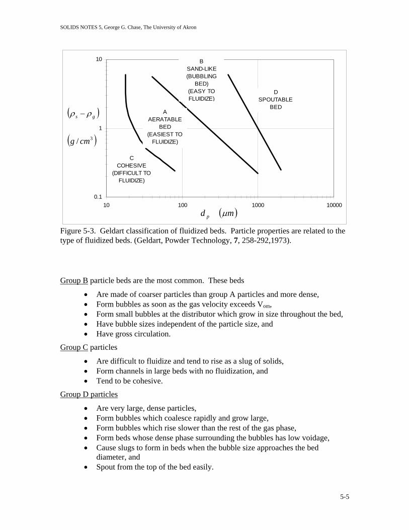
SOLIDS NOTES 5, George G. Chase, The University of Akron
0.1
1
10
10 100 1000 10000
DSPOUTABLE
BED
BSAND-LIKE(BUBBLING
BED)(EASY TO FLUIDIZE)
AAERATABLE
BED(EASIEST TO
FLUIDIZE)
CCOHESIVE
(DIFFICULT TO FLUIDIZE)
( )
( )3/ cmg
gs ρρ −
( )md p µ
Figure 5-3. Geldart classification of fluidized beds. Particle properties are related to the type of fluidized beds. (Geldart, Powder Technology, 7, 258-292,1973).
Group B particle beds are the most common. These beds
• Are made of coarser particles than group A particles and more dense, • Form bubbles as soon as the gas velocity exceeds Vom, • Form small bubbles at the distributor which grow in size throughout the bed, • Have bubble sizes independent of the particle size, and • Have gross circulation.
Group C particles
• Are difficult to fluidize and tend to rise as a slug of solids, • Form channels in large beds with no fluidization, and • Tend to be cohesive.
Group D particles
• Are very large, dense particles, • Form bubbles which coalesce rapidly and grow large, • Form bubbles which rise slower than the rest of the gas phase, • Form beds whose dense phase surrounding the bubbles has low voidage, • Cause slugs to form in beds when the bubble size approaches the bed
diameter, and • Spout from the top of the bed easily.
5-5

SOLIDS NOTES 5, George G. Chase, The University of Akron
Kunii and Levenspeil present a more generalized diagram (ibid, Figure 16) for classifying fluidization regimes. They plot a dimensionless particle diameter, versus a dimensionless velocity where
d p *u *
( ) ( )d d
gC Rp p
pD ep*=
−⎡
⎣⎢⎢
⎤
⎦⎥⎥
=ρ ρ ρ
µ 2
13
34
21
3 (5-1)
and
( )u ug
RC
p
ep
D
*=−
⎡
⎣
⎢⎢
⎤
⎦
⎥⎥
=⎛
⎝⎜
⎞
⎠⎟
ρ
µ ρ ρ
21
3 134
3. (5-2)
With the data arranged this way they identify several interesting features including:
• Geldart’s classification, • Terminal velocity, , ut
• Minimum fluidization velocity, , and umf
• Types of fluidization (spouted beds, bubbling, fast fluidized beds and pneumatic transport).
5.5 Prediction of Minimum Fluidization A minimum velocity is needed to fluidized a bed. If the velocity is too small the bed stays fixed and operates as a packed bed.
Recall the Ergun Equation is presented in dimensionless form in Eq.(4-25) which relates the pressure drop to the flow rate through a packed bed. At the onset of fluidization the particles are still close enough together that the pressure drop is related to the velocity by the Ergun Equation. Also, a free body diagram tells us that the force due to pressure drop is also related to the net weight of the solids in the bed
( )( )( )∆P A A Lggp f f
c
= − −ρ ρ ε1 (5-3)
where the right side of Eq.(5-3) is the weight of the solids minus the buoyant force due to the displaced fluid. The subscripts f mean that the quantity is for a fluidized bed.
If we consider a total mass balance on the solids, assuming that no solids are entrained and carried out of the bed, then the total mass of solids is constant given by
( )M ALsolids p f f= − =ρ ε1 constant (5-4)
5-6

SOLIDS NOTES 5, George G. Chase, The University of Akron
At different fluidization rates the porosity, ε , and the bed height, , vary but the rest of the terms in Eq.(5-4) are constants. This means that at the porosities and bed heights at flow rates 1 and 2 are related by
L
( ) ( )1 11 1 2 2− = −ε εL L . (5-5)
For liquids and for gases, as long as the pressure drop is small, the fluid phase density is constant. Hence, the right hand side of Eq.(5-3) is constant and thus the pressure drop in a fluidized bed is constant independent of the velocity.
Experimental data show this to be true. A typical plot of the pressure drop versus the velocity is shown in Figure 5-4.
Substitution of Eq.(5-3) into Eq.(4-25) gives the modified Ergun Equation for fluidized beds
( )
GAfepf
f
fepf
NRR =Φ
−+
Φ 232
3
118080.1ε
εε
(5-6)
where
RV d
ep f
of p=ρ
µ (5-7)
and ( )
Nd g
GAp p
=−3
2
ρ ρ ρ
µ. (5-8)
LOOSE PACKED
DENSE PACKED(FIRST TIME BED IS FLUIDIZED)
V
FLUIDIZED BEDOPERATION
P
PACKED BEDOPERATION
V m
Figure 5-4. Typical pressure drop versus velocity plot for fluidized beds. Initially if the bed is densely packed the pressure drop overshoots the fluidization pressure until the particles separate and fluidize.
5-7

SOLIDS NOTES 5, George G. Chase, The University of Akron
For small , such as with very small particles, we can neglect the term and
get the Blake-Kozeny expression
Rep f<1 Rep f
2
( )
GAfepf
f NR =Φ
−23
1180ε
ε for Rep f
<1 (5-9)
or ( )
( )f
fppof
gdV
εε
µρρ
−
Φ−=
1180
232
(5-10)
which relates the fluidization velocity to the void volume fraction of the expanded bed.
To estimate the onset of fluidization, we can estimate the minimum fluidization conditions. The minimum fluidization porosity, mε , can be estimated from Figure 4-1 for loose packing and known sphericity, Φ . Using this value for mε we can solve the Ergun Equation, Eq.(5-6) for the minimum fluidization velocity, . moV
When mε and are not known, we can still estimate the minimum fluidization velocity. The modified Ergun Equation, Eq.(5-6) is rewritten as
Φ
(5-11) GAmepmep NRKRK =+ 12
2
where ( )
2311180Φ−
=m
mKε
ε and
Φ= 32
8.1
m
Kε
Wen and Yu (AIChE J, 12(3), 610-612, 1966) noted that and stay nearly constant over a wide range of particles and for
K1 K 2
4000001.0 <<mepR ; thus giving a prediction of
with a 34% standard deviation. Vo mf
Equation (5-11) can be solved for the minimum fluidization velocity, provided and are known, gives
K1
K 2
⎟⎟⎠
⎞⎜⎜⎝
⎛−+⎟⎟
⎠
⎞⎜⎜⎝
⎛=
2
1
2
2
2
1
21
2 KK
NKK
KR GAmep (5-12)
for which Wen and Yu determined KK
1
22337
⎛⎝⎜
⎞⎠⎟ = . and
10 0408
2K= . .
Since the work of Wen and Yu, others have determined values for and . Table 5-1 summarizes values for fine and coarse particles.
K1 K 2
5-8
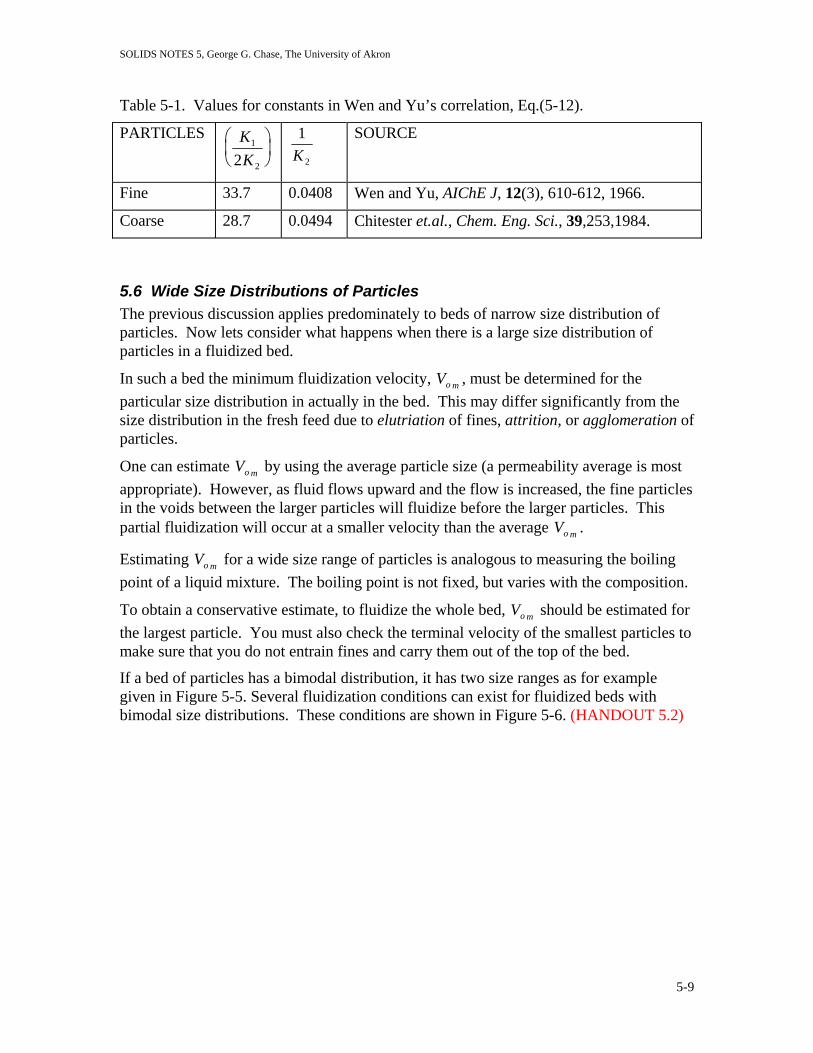
SOLIDS NOTES 5, George G. Chase, The University of Akron
Table 5-1. Values for constants in Wen and Yu’s correlation, Eq.(5-12).
PARTICLES KK
1
22⎛⎝⎜
⎞⎠⎟
1
2K
SOURCE
Fine 33.7 0.0408 Wen and Yu, AIChE J, 12(3), 610-612, 1966.
Coarse 28.7 0.0494 Chitester et.al., Chem. Eng. Sci., 39,253,1984.
5.6 Wide Size Distributions of Particles The previous discussion applies predominately to beds of narrow size distribution of particles. Now lets consider what happens when there is a large size distribution of particles in a fluidized bed.
In such a bed the minimum fluidization velocity, , must be determined for the particular size distribution in actually in the bed. This may differ significantly from the size distribution in the fresh feed due to elutriation of fines, attrition, or agglomeration of particles.
moV
One can estimate by using the average particle size (a permeability average is most appropriate). However, as fluid flows upward and the flow is increased, the fine particles in the voids between the larger particles will fluidize before the larger particles. This partial fluidization will occur at a smaller velocity than the average .
moV
moV
Estimating for a wide size range of particles is analogous to measuring the boiling point of a liquid mixture. The boiling point is not fixed, but varies with the composition.
moV
To obtain a conservative estimate, to fluidize the whole bed, should be estimated for the largest particle. You must also check the terminal velocity of the smallest particles to make sure that you do not entrain fines and carry them out of the top of the bed.
moV
If a bed of particles has a bimodal distribution, it has two size ranges as for example given in Figure 5-5. Several fluidization conditions can exist for fluidized beds with bimodal size distributions. These conditions are shown in Figure 5-6. (HANDOUT 5.2)
5-9

SOLIDS NOTES 5, George G. Chase, The University of Akron
Particle Size
Number
Bimodal Distribution
Figure 5-5. Bimodal distribution of particle sizes showing two peaks (modes) in the number of particles of each size.
5-10

SOLIDS NOTES 5, George G. Chase, The University of Akron
d large
dp avg
p
d smallp
ε
d large
FLOW
d small
p
p
(a) Complete segregation of particles into a region of predominately
small particles and a region of predominately large particles. The segregation may also be characterized by an abrupt change in bed porosity.
d large
dp avg
p
ε
d smallp
d mixedp
d large
FLOW
p
d small
d mixed
p
p
(b) Partial segregation into two regions with different particle sizes
separated by a layer of mixed particle sizes.
dp avg
d mixedp
ε FLOW
d mixed.p
(c) No segregation of particles. The average particle size may gradually
vary throughout the depth of the bed.
Figure 5-6. Fluidized beds with bimodal size distribution.
5-11

SOLIDS PROCESSING HANDOUTS, George G. Chase, The University of Akron
HANDOUT 5.1
0.1
1
10
10 100 1000 10000
DSPOUTABLE
BED
BSAND-LIKE(BUBBLING
BED)(EASY TO FLUIDIZE)
AAERATABLE
BED(EASIEST TO
FLUIDIZE)
CCOHESIVE
(DIFFICULT TO FLUIDIZE)
( )
( )3/ cmg
gs ρρ −
( )md p µ
Figure 5-3. Geldart classification of fluidized beds. Particle properties are related to the type of fluidized beds. (Geldart, Powder Technology, 7, 258-292,1973).
1
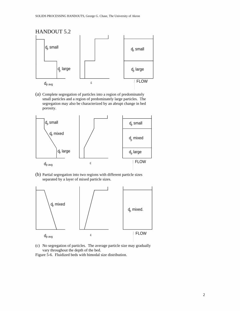
SOLIDS PROCESSING HANDOUTS, George G. Chase, The University of Akron
HANDOUT 5.2
d large
dp avg
p
d smallp
ε
d large
FLOW
d small
p
p
(a) Complete segregation of particles into a region of predominately
small particles and a region of predominately large particles. The segregation may also be characterized by an abrupt change in bed porosity.
d large
dp avg
p
ε
d smallp
d mixedp
d large
FLOW
p
d small
d mixed
p
p
(b) Partial segregation into two regions with different particle sizes
separated by a layer of mixed particle sizes.
dp avg
d mixedp
ε FLOW
d mixed.p
(c) No segregation of particles. The average particle size may gradually
vary throughout the depth of the bed. Figure 5-6. Fluidized beds with bimodal size distribution.
2

Solids Notes 6, George G. Chase, The University of Akron
6. ELUTRIATION OF PARTICLES FROM FLUIDIZED BEDS Elutriation is the process in which fine particles are carried out of a fluidized bed due to the fluid flow rate passing through the bed. Typically, fine particles are elutriated out of a bed when the superficial velocity through the bed exceeds the terminal velocity of the fines in the bed. However, elutriation can also occur at slower velocities. Fine particles are present in fluidized beds from several sources:
Feed streams Mechanical attrition or breakage of larger particles Temperature stress cracking Size reduction due to chemical reactions, shrinkage, etc.
When fines elutriation is a significant problem and modifications to the bed design cannot aid in reducing the problem, fines can often be recovered such as with cyclones or hydrocyclones. Leva (Chem. Engr. Prog., 47, 39, 1951) measured the rate of elutriation (total mass per time) from a bed of particles with a bimodal size distribution. He found that
(1) When the column height above the bed is small, the elutriation rate is high. But if the height exceeds a certain minimum size then the rate is a constant minimum value (Figure 6-1).
This occurs because small particles that are expelled from the top of the bed have high velocities and they require greater distance to slow down and turn around to return to the bed.
(2) The elutriation process causes a decrease in particle concentration. The
concentrations may be empirically modeled by an Arrhenius type expression as
MteCC −= 0 (6-1)
where C = concentration at time, t; Co is the initial concentration; and M is an empirical constant.
6-1
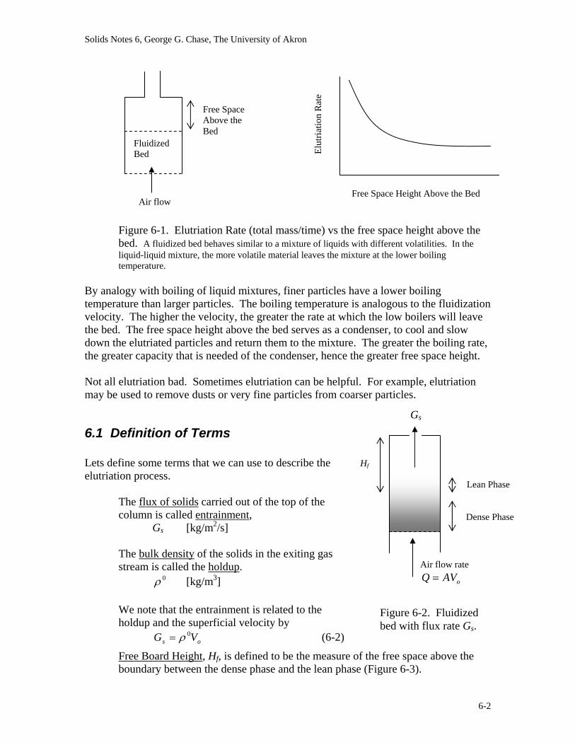
Solids Notes 6, George G. Chase, The University of Akron
Fluidized Bed
Air flow
Figure 6-1. Elutriation Rate (total mass/time) vs the free space height above the bed. A fluidized bed behaves similar to a mixture of liquids with different volatilities. In the liquid-liquid mixture, the more volatile material leaves the mixture at the lower boiling temperature.
By analogy with boiling of liquid mixtures, finer particles have a lower boiling temperature than larger particles. The boiling temperature is analogous to the fluidization velocity. The higher the velocity, the greater the rate at which the low boilers will leave the bed. The free space height above the bed serves as a condenser, to cool and slow down the elutriated particles and return them to the mixture. The greater the boiling rate, the greater capacity that is needed of the condenser, hence the greater free space height. Not all elutriation bad. Sometimes elutriation can be helpful. For example, elutriation may be used to remove dusts or very fine particles from coarser particles.
6.1 Definition of Terms Lets define some terms that we can use to describe the elutriation process.
The flux of solids carried out of the top of the column is called entrainment, Gs [kg/m2/s] The bulk density of the solids in the exiting gas stream is called the holdup. [kg/m0ρ 3] We note that the entrainment is related to the holdup and the superficial velocity by (6-2) os VG 0ρ=
Free Board Height, Hf, is defined to be the measure of the free space above the boundary between the dense phase and the lean phase (Figure 6-3).
Free Space Height Above the Bed
Gs
Air flow rate
oAVQ =
Hf
Dense Phase
Lean Phase
Figure 6-2. Fluidized bed with flux rate Gs.
Elut
riatio
n R
ate
Free Space Above the Bed
6-2

Solids Notes 6, George G. Chase, The University of Akron
For design, we need to know the rate of entrainment and the size distribution of the entrained particles in relation to the size of the particles in the bed. A fluidized bed usually has two regions or phases: dense bubbling phase and lean dispersed phase (Figure 6-2).
Air flow rate
oAVQ =
Dense Phase
TDH Both fines and coarse particles are entrained in this region
Only fines are entrained in this region
Bulk density, 0ρ
Hf
Figure 6-3. Both fines and coarse particle are entrained in the Transport Disengagement Height (TDH) region. Above the TDH only fines are entrained.
The Transport Disengagement Height (TDH) is the height above the dense-phase/lean-phase boundary above which entrainment and bulk density do not change appreciably. TDH depends upon the superficial velocity and the particle properties. The TDH is the height at which the kinetic energies of particles due to the collisions in the bed has been expended against gravity potential, and the coarse particles whose terminal velocities are greater than the superficial velocity are able to fall back down to the bed. The fine particles, whose terminal velocities are less than the superficial velocity, continue to be entrained out of the column. When Hf > TDH then the holdup and entrainment rates are close to their minimums. Usually Hf = TDH is the most economical design height for the fluidized bed. If Hf < TDH then coarse particles will be carried out of the column.
6-3

Solids Notes 6, George G. Chase, The University of Akron
6.2 Estimation of TDH for Geldart A Particles. For beds of fine particles (Geldart A classification, see Fluidization notes 5) there are several methods discussed in literature. Kunii and Levenspiel give a good review of this literature. In these notes you are only given a brief introduction. METHOD 1. Zenz and Weil (AICHE J. 4, 472, 1958) proposed a correlation between dimensionless TDH and the vessel diameter. For catalyst pellets in 20 to 150 micron size range, on a log-log plot, the relation between the dimensionless TDH and the vessel diameter are nearly linear (see Kunii and Levenspiel Figure 5 page 173) as indicated in Figure 6-4.
Vo
dt
TDH
/dt
Figure 6-4. Dimensionless TDH/dt vs vessel diameter, dt. We can model the data on the chart in the form of ( ) ( ) ( )bLogdmLogdTDHLog tt +=/ (6-1) where dt is the vessel diameter. Taking data points from the chart and plotting them we can curve fit to find the parameters m and b: (6-2) 587.0115.0 −−= oVm (6-3) oVb 64.4= Finally, we take the above equations and try to compress the chart by plotting the dimensionless TDH/dt versus the Froude Number, to get the plot shown in Figure 6-5. (HANDOUT 6.1)
gdVF tor //2=
6-4

Solids Notes 6, George G. Chase, The University of Akron
y = 23.171xR2 = 0.8972
0
5
10
15
20
25
30
0 0.2 0.4 0.6 0.8 1 1.2 1.4
Vo2/dt/g
TDH
/dt
Figure 6-5. Dimensionless TDH/dt versus Froude Number. If we take the linear fit in Figure 6-5 to represent the material behavior, then we can relate
gd
Vd
TDH
t
o
t
2
171.23= (6-4)
or, upon rearrangement, we get
0432.0constant 2
==gTDH
Vo (6-5)
The constant in Eq.(6-5) is likely to be material specific. Fournol et.al. (Can. J. Chem. Engr., 51, 401, 1973) independently determined, for a fluidized bed of fine catalyst particles, dp=58 microns, the TDH for this material to be given by
.0010 2
=gTDH
Vo (6-6)
6-5

Solids Notes 6, George G. Chase, The University of Akron
6.3 Entrainment Rate from Tall Vessels There are several methods for estimating entrainment rates. Following the work by Zenz et.al. (AICHE J., 4, 472, 1958; and Fluidization III, Grace & Matsen, eds., Plenum, N.Y. 1980) we assume that the flux rate of solid size dpi is proportional to its mass fraction, xi, (6-7) *
siisi GxG = where is the flux rate from an imaginary bed of all particles of size d*
siG pi. This approach extends the analogy between fluidized beds and boiling of a liquid mixture (discussed in the introduction to Section 6). Raoult’s Law for an ideal fluid mixture (R.E. Balzhiser, M.R. Samuels, and J.D. Eliassen, Chemical Engineering Thermodynamics, Prentice Hall, Englewood Cliffs, New Jersey, 1972) equates the partial pressure of component i in the vapor phase to the mole fraction in the liquid phase times the pure fluid vapor pressure. (6-8) *
iii PxP = hence, the flux rates are analogous to the vapor pressures. The procedure to determine the flux rate from a bed with known particle size distribution is as follows:
1. Divide the size distribution into narrow intervals and find which intervals have terminal velocities greater than the superficial velocity (these are the particles that are entrained, because Hf > TDH).
2. Find for each size range. *siG
3. The total entrainment is given by ∑= *
siis GxG (6-9) In terms of a continuous size distribution, P(dp), the total entrainment rate is given by
∫= ppsis dddPGG )(* (integration over all particles entrained) (6-10) To apply this procedure, a correlation such as shown in Figure 6-6 is required to find
. *siG
6-6

Solids Notes 6, George G. Chase, The University of Akron
6-7
1
10
100
1000
10000
0.01 0.1 1 10 100
1
10
100
1000
10000
og
s
uG
ρ
*
( )p
to
gduu 2−
p
o
gdu 2510
Geldart A beds with most particles entrainable
Fines removed from larger particle beds
Figure 6-6. Data taken from Kunii & Levenspeil, Fluidization Engineering, 2ed, Butterworth, Boston, 1991 (figure 6 page 175). From this plot the value of G*s may be determined for Geldart A particles and for fines removed from larger particle beds. For Geldart class B, C, or D particles (the larger particles) other predictive models are available. Recommended references: Kunii and Levenspiel (J. Chem. Eng. Japan, 2, 84, 1969) Lewis et. al. (Chem. Eng. Prog. Symposium Series, 58 (38), 65, 1962) Wen and Chen (AICHE J., 28, 117, 1982) Kunii and Levenspiel (Fluidization Engineering, 2ed, Butterworth, Boston, 1991).

SOLIDS PROCESSING HANDOUTS, George G. Chase, The University of Akron
HANDOUT 6.1
y = 23.171xR2 = 0.8972
0
5
10
15
20
25
30
0 0.2 0.4 0.6 0.8 1 1.2 1.4
Vo2/dt/g
TDH
/dt
Figure 6-5. Dimensionless TDH/dt versus Froude Number.
1
10
100
1000
10000
0.01 0.1 1 10 100
1
10
100
1000
10000
og
s
uG
ρ
*
( )p
to
gduu 2−
p
o
gdu 2510
Geldart A beds with most particles entrainable
Fines removed from larger particle beds
Figure 6-6. Data taken from Kunii & Levenspeil, Fluidization Engineering, 2ed, Butterworth, Boston, 1991 (figure 6 page 175). From this plot the value of G*s may be determined for Geldart A particles and for fines removed from larger particle beds.
1

SOLIDS NOTES 7, George G. Chase, The University of Akron
7. SOLID/LIQUID SEPARATIONS
7.1 INTRODUCTION There are large varieties of separation equipment available to industry for Solid/Liquid separations. A frequent question is: “Which is the right choice for my application”? A number of authors have published selection guides to help the practicing engineers. Because of its complexity an number of approaches have been developed. As part of the introduction I summarize these approaches for you. REFERENCES: 1. D.B. Purchase, Solid/Liquid Separation Technology, Uplands Press, Croydon, England, 1981. 2. F.M. Tiller, “Bench Scale Design of SLS Systems,” Chem. Eng., 81, 117-119, 1974. 3. M. Ernst, R.M. Talcott, H.C. Romans, G.R.S. Smith, “Tackle Solid-Liquid Separation Problems,”
Chem. Eng. Prog., 87(7), 22-28, 1991. There are four stages to S/L Separations. Not all of these stages are present in all processes. These stages are: PRETREATMENT SOLIDS CONCENTRATION SOLIDS SEPARATIONS POST TREATMENT Table 7-1 further breaks these topic down into sub categories (HANDOUT 7.1).
7-1

SOLIDS NOTES 7, George G. Chase, The University of Akron
Table 7-1. Four Stages of Solid Liquid Separations. PRETREATMENT
To increase particle size, reduce viscosity.
CHEMICAL PHYSICAL coagulation crystallization flocculation aging freezing/heating filteraid admix SOLIDS CONCENTRATION
To reduce the volume of material to process.
CLARIFICATION THICKENING gravity sedimentation gravity sedimentation cross flow filtration cyclones periodic pressure filters SOLIDS SEPARATION
To separate the solids from the liquid; to form cakes of dry solids or to produce particulate free liquid.
CLARIFICATION FILTRATION CENTRIFUGATION granular bed vacuum sedimenting centrifuge precoat drum gravity filtering centrifuge pressure cyclone expression POST TREATMENT
To remove solubles, remove moisture, reduce cake porosity, or prepare material for downstream processes.
PHYSICAL washing drying repulping deliquoring
7-2

SOLIDS NOTES 7, George G. Chase, The University of Akron
7.2 Pretreatment The cost of S/L separations is directly related to the volume of material that must be processed. Pressurized equipment such as pressure filters are more expensive to operate than thickeners, for example. Hence, there is incentive to optimize the process by setting up the equipment in series. (HANDOUT 7.2) For example, suppose you have slurry feed that is 1% solids. You run this slurry through a thickener that concentrates it to 10% solids, followed by a filter centrifuge that filters it to 25% solids. The centrifuge is then used to deliquor the cake with a resulting cake of 50% solids. In each of these steps how much of the original slurry is processed and how much liquid is removed? Basis: 100 unit volumes of slurry feed Table 7-2. Effect of concentrating a slurry on the volume. Step Solids
Volume % Volume Solids
Volume Liquid In Mixture
Volume Liquid Removed
% Liquid Removed from Feed
Volume of Mixture (After Treatment)
Feed
1 1 99 0 0 100
Thickener 10 1 9 90 90/99 = 90.9
10
Filter
25 1 3 6 6/99 = 6.1
4
Deliquoring 50 1 1 2 2/99 = 2.0
2
Hence, you can see that even though the thickener only concentrated the solids from 1 to 10%, 91% of the liquid was removed and the mixture yet to be treated was only 10% of the volume of the original feed.
Thickener
Filter Cost
s Size
Figure 7-1. Relative costs of filters and thickeners as related to size.
Pretreatment aids in reducing costs by prethickening the slurry, as in the previous example. There are a number of pretreatment techniques that can be used and that have this effect. These pretreatment techniques are summarized in Table 7-3. (HANDOUT 7.1)
Table 7-3. Pretreatment techniques.
7-3
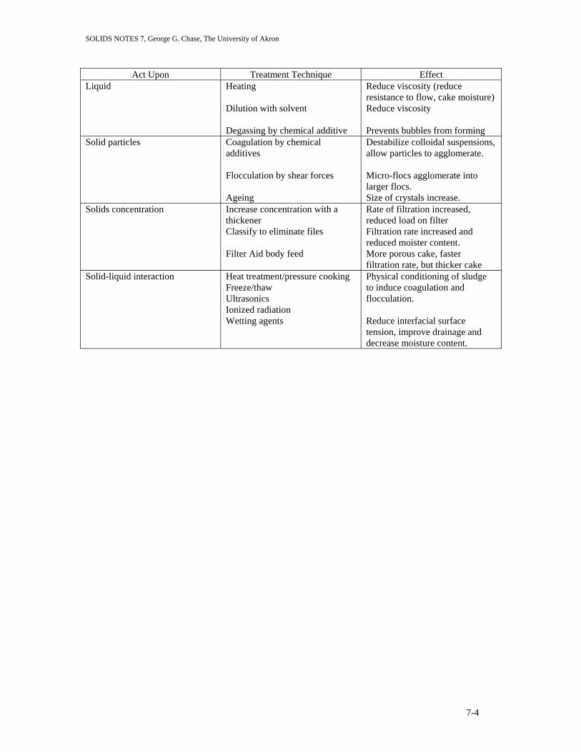
SOLIDS NOTES 7, George G. Chase, The University of Akron
Act Upon Treatment Technique Effect Liquid Heating
Dilution with solvent Degassing by chemical additive
Reduce viscosity (reduce resistance to flow, cake moisture) Reduce viscosity Prevents bubbles from forming
Solid particles Coagulation by chemical additives Flocculation by shear forces Ageing
Destabilize colloidal suspensions, allow particles to agglomerate. Micro-flocs agglomerate into larger flocs. Size of crystals increase.
Solids concentration Increase concentration with a thickener Classify to eliminate files Filter Aid body feed
Rate of filtration increased, reduced load on filter Filtration rate increased and reduced moister content. More porous cake, faster filtration rate, but thicker cake
Solid-liquid interaction Heat treatment/pressure cooking Freeze/thaw Ultrasonics Ionized radiation Wetting agents
Physical conditioning of sludge to induce coagulation and flocculation. Reduce interfacial surface tension, improve drainage and decrease moisture content.
7-4
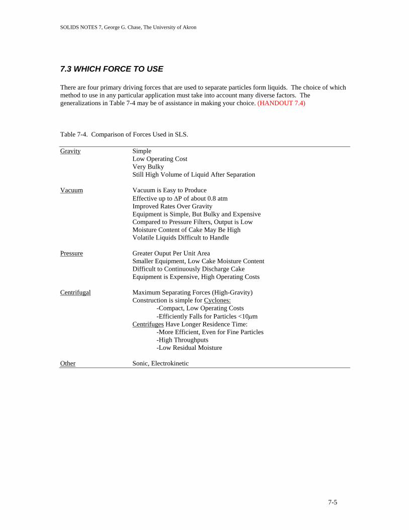
SOLIDS NOTES 7, George G. Chase, The University of Akron
7.3 WHICH FORCE TO USE There are four primary driving forces that are used to separate particles form liquids. The choice of which method to use in any particular application must take into account many diverse factors. The generalizations in Table 7-4 may be of assistance in making your choice. (HANDOUT 7.4) Table 7-4. Comparison of Forces Used in SLS. Gravity Simple Low Operating Cost Very Bulky Still High Volume of Liquid After Separation Vacuum Vacuum is Easy to Produce
Effective up to ∆P of about 0.8 atm Improved Rates Over Gravity Equipment is Simple, But Bulky and Expensive Compared to Pressure Filters, Output is Low Moisture Content of Cake May Be High Volatile Liquids Difficult to Handle
Pressure Greater Ouput Per Unit Area Smaller Equipment, Low Cake Moisture Content Difficult to Continuously Discharge Cake Equipment is Expensive, High Operating Costs Centrifugal Maximum Separating Forces (High-Gravity) Construction is simple for Cyclones: -Compact, Low Operating Costs -Efficiently Falls for Particles <10µm Centrifuges Have Longer Residence Time: -More Efficient, Even for Fine Particles -High Throughputs -Low Residual Moisture Other Sonic, Electrokinetic
7-5

SOLIDS NOTES 7, George G. Chase, The University of Akron
7.4 RANGE OF APPLIED FORCES AND COMPACTIBILITY As the slurries are thickened, and as cakes are formed, the mixture transitions from a condition in which there is a relatively large mean-free distance between particles, to one in which particles are in contact. (HANDOUT 7.5)
Low Concentration Slurry, Little Particle-Particle Contact
Electrical Field Surrounding the particles
High Concentration Mixture (Low Porosity) With Significant Particle-Particle Contact
Figure 7-2. Particle contact as a function of concentration. Surface charges and electrostatic forces can keep particles separated, requiring compressive forces to push particles together.
Especially in filter cakes, the drag force of the fluid on the particles can cause significant stresses to develop on the skeletal matrix of the solids. Compaction occurs when particles rearrange their relative positions to each other to pack more closely together. A certain amount of force is required to squeeze the fluid phase out of the pore spaces between the particles. The smaller the pores (typically with smaller particles) the greater the force required. However, very small particles can also have large repulsive forces due to surface charges and electrostatic effects. One measure of the surface charge is Zeta Potential. At the isokinetic point the zeta potential is zero and the particles can pack more closely together with the least amount of force (R.J. Wakeman and E.S. Tarleton, Filtration: Equipment Selection Modeling and Process Simulation, Elsevier, Oxford, 1999). Zeta potential is influenced by material properties of the particles as well as the pH and salt concentration of the solution. Several instruments are available for measuring zeta potential such as the Zeta Meter and the Anton Paar EKA. Typical zeta potential values are shown in Figures 7-3 and 7-4. (HANDOUT 7.6) Fibrous materials are also known to compact. Their compaction may be a combination of surface charges and bending of the fibers. This stress on the solids matrix can cause the matrix to compact. The degree of compactability has a profound effect on the way the solid matrix reacts to changes in the applied pressure. Some data reported in literature is shown in Figure 7-5. (HANDOUT 7.7)
7-6
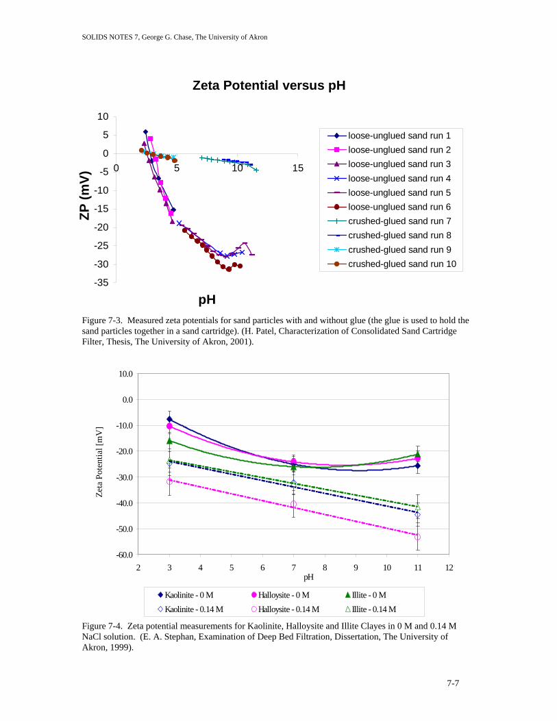
SOLIDS NOTES 7, George G. Chase, The University of Akron
Zeta Potential versus pH
-35
-30
-25
-20
-15
-10
-5
0
5
10
0 5 10 15
pH
ZP (m
V)
loose-unglued sand run 1loose-unglued sand run 2loose-unglued sand run 3loose-unglued sand run 4loose-unglued sand run 5loose-unglued sand run 6crushed-glued sand run 7crushed-glued sand run 8crushed-glued sand run 9crushed-glued sand run 10
Figure 7-3. Measured zeta potentials for sand particles with and without glue (the glue is used to hold the sand particles together in a sand cartridge). (H. Patel, Characterization of Consolidated Sand Cartridge Filter, Thesis, The University of Akron, 2001).
-60.0
-50.0
-40.0
-30.0
-20.0
-10.0
0.0
10.0
2 3 4 5 6 7 8 9 10 11 12pH
Zeta
Pot
entia
l [m
V]
Kaolinite - 0 M Halloysite - 0 M Illite - 0 MKaolinite - 0.14 M Halloysite - 0.14 M Illite - 0.14 M
Figure 7-4. Zeta potential measurements for Kaolinite, Halloysite and Illite Clayes in 0 M and 0.14 M NaCl solution. (E. A. Stephan, Examination of Deep Bed Filtration, Dissertation, The University of Akron, 1999).
7-7

SOLIDS NOTES 7, George G. Chase, The University of Akron
0.3
0.4
0.5
0.6
0.7
0.8
0.9
1
1 10 100 1000 10000
Applied Compressive Stress, kPa
Poro
sity
Grade E Carbonyl IronKaolinLatexTalcSupercelFine Silica
Figure 7-5. Compressibility of packed beds of selected materials (H.P. Grace, “Resistance and Compressibility of Filter Cakes (Part I and II), Chem. Eng. Prog., 49, 303-318, 367-377, 1953).
The carbonyl iron typifies particles which form incompressible beds and have sufficient internal strength to resist crushing. The Supercel (processed diatomaceous earth) is slightly compactable with a fragile structure which disintegrates under sufficient pressure or shear force. Its open structure results from the unusual shape of diatoms which are the basic raw material. The kaolin is moderately compactable. The fine silica and talc are highly compactable, and the flocculated latex is super-compactable. In sedimentation and thickening, the forces occur in the low pressure range. If a material is highly compactable, such as a floc, then we typically see changes in porosity in the range of 0.9 to 0.8. Particles flow into unoccupied voids and flocs are squeezed. At the other extreme, in high-pressure expression, the effective pressure may range up to hundreds of atmospheres. At his high pressure range the compaction occurs due to particle deformation and crushing (where the material’s intrinsic coefficient of elasticity, ultimate strength, and loss of bound water are important). A diagram of the ranges of pressures encountered in SLS and corresponding porosities are shown in the Figure 7-6. (HANDOUT 7.7)
7-8

SOLIDS NOTES 7, George G. Chase, The University of Akron
0
0.2
0.4
0.6
0.8
1
0.01 0.1 1 10 100 1000
Compressive Stress, ATM
Poro
sity
THICKENER
GRAVITY FILTER
VACUUM FILTER
PRESSURE FILTER
CENTRIFUGE
EXPRESSION
PARTICLEDEFORMATION
Figure 7-6. Compressive Stress relation to separation operation. (F. Tiller and W. Li, Theory and Practice of Solid/Liquid Separation, 4th ed., University of Houston, 2002.
7.5 Selecting the Right Equipment It is rare if ever true that there is an absolute “right” choice for SLS equipment, which is superior in all respects to other equipment. This is due to the multiple operating factors and that often the “right” choice is a combination of 2 or more items operating in series or in parallel. Because of this difficulty a master selection chart is yet to be developed. On the other hand, it is possible to separate out the “wrong” choices. It is in this respect that the available charts are of the most value. Table 7-5 gives a selection chart for selecting between different types of filters. Table 7-6 gives a similar chart for selecting between different types of centrifuges. These charts are based on typical operating ranges in solid mass fractions and particle sizes. The charts also give a ranking or score of 0 (worst) to 9 (best) on four different criteria: crystal breakage (ie, least amount of breakage of crystal particles), clarity of the filtrate, washability of the formed cake, and cake dryness. (HANDOUTS 7.8, 7.9) Other similar tables are available in literature (D.B. Purchas, Solid/Liquid Separation Technology, Uplands Press, Croydon, 1981) that considers criteria such as power, space, and costs.
7-9

SOLIDS NOTES 7, George G. Chase, The University of Akron
Table 7-5. Filter Selection Chart. (data from D.B. Purchas, Solid/Liquid Separation Technology, Uplands Press, Croydon, 1981, E. Davies, Filtr., Sep 7(1) 76-79, 1970).
TYPICAL OPERATING RANGE PERFORMANCE SCORE 0 TO 9
(9 IS BEST) Filter
% (mass) OF SOLIDS IN THE FEED
PARTICLE SIZE OF SOLIDS, MICRONS
CA
KE D
RY
NESS
WA
SH
PERFO
RM
AN
CE
FILTRA
TE C
LAR
ITY
CR
YSTA
L B
REA
KA
GE
LEAF
0.01 – 1 0.5 TO 500 5-6 6 7-8 8
PLATE
0.001 – 0.1 0.5 – 100 5 8 8-9 8
CANDLE/PRECOAT
0.001 - 0.1 0.5 - 200 5 7 7-8 8
CARTRIDGE
0.001 – 0.1 0.5 – 80 5 7 7-9 8
FILTER PRESS
0.001 – 50 1 – 100 6-7 7 7-8 8
SHEET FILTER
0.001 – 1 0.1 – 80 5-6 7 8-9 -
STRAINER
0.001 – 0.05 5 – 500 - - 7 -
VACUUM DRUM
2 – 90 1 –500 4-5 7 7-8 8
VACUUM DRUM WITH PRECOAT
0.005 – 0.2 0.5 – 100 - - 8 -
VACUUM DISC
2 – 90 1 – 500 2-3 2 6 8
BAND, PAN, TABLE
5 – 90 5 – 100,000 5-7 9 7 8
WATER SCREEN
0.001 – 0.1 20 – 100,000 - - 6 -
DEEP BED
0.001 – 0.1 0.1 – 80 - - 7-9 -
7-10

SOLIDS NOTES 7, George G. Chase, The University of Akron
Table 7-6. Centrifuge Selection Chart (data from D.B. Purchas, Solid/Liquid Separation Technology, Uplands Press, Croydon, 1981; E. Davies, Filtr., Sep 7(1) 76-79, 1970). ).
TYPICAL OPERATING RANGE PERFORMANCE SCORE 0 TO 9
(9 IS BEST) Centrifuge
% (mass) OF SOLIDS IN THE FEED
PARTICLE SIZE OF SOLIDS, MICRONS
CA
KE D
RY
NESS
WA
SH
PERFO
RM
AN
CE
FILTRA
TE C
LAR
ITY
CR
YSTA
L B
REA
KA
GE
PUSHER
8 – 90 50 – 80,000 9 5 4 4
PEELER/SCRAPER
5 – 80 2 – 20,000 9 6 5 5
WORM SCREEN
3 – 90 100 – 20,000 9 5 4 4
OSCILLATING SCREEN
3 – 90 100 – 30,000 7-9 5 4 3
BASKET
2 –80 2 – 20,000 9 6 5 6
CONICAL SCREEN
5 – 90 100 – 20,000 7 - 5 7
SCREEN BOWL
2 – 70 90 – 20,000 6 5 4 5
DECANTER
2 – 70 1 – 20,000 4 3 4 -
TUBULAR BOWL
0.01 – 1 0.1 – 100 - - 6-7 -
DISC (MANUAL)
0.003 –0.08 0.1 – 100 3 - 6-7 -
DISC (SELF CLEANING)
0.02 – 2 0.1 – 100 3 - 6-7 -
NOZZLE BOWL
0.05 – 5 0.1 – 100 3 - 6-7 -
7-11

SOLIDS NOTES 7, George G. Chase, The University of Akron
Another way to select equipment type is on the rate of cake formation as suggested by F. Tiller in Table 7-7. (HANDOUT 7.10) Table 7-7. Selection based on cake formation rate (F. Tiller, Chem. Eng. Progr. Oct. 1977, 65-76). Cake Formation Rate (rate at which cake height grows in a gravity filter).
Separation type Equipment
0.1 to 10 cm/sec Rapid Filtering Gravity pans; screens; horizontal belt or top-feed drum filter; continuous feed pusher centrifuge
0.1 to 10 cm/min Medium Filtering Vacuum drum, disc, horizontal belt, pan filters, peeler centrifuge
0.1 to 10 cm/hr Slow Filtering Pressure filters, disc and tubular centrifuges, sedimenting centrifuges
Negligible cake Clarification Cartridges, granular beds, precoat drums, filter aid admix
A paper by Ernst et.al. (M. Ernst, R.M. Talcott, H.C. Romans, G.R.S. Smith, Tackle Solid-Liquid Separation Problems, CEP, 87(7), 22-28, 1991). The selection method eliminates unsuitable equipment and it ranks suitable equipment on how well they can perform the separation. This ranking allows us to narrow down options so that only a small number of types of equipment need to be evaluated.
7-12

SOLIDS PROCESSING HANDOUTS, George G. Chase, The University of Akron
HANDOUT 7.1 Table 7-1. Four Stages of Solid Liquid Separations PRETREATMENT
To increase particle size, reduce viscosity.
CHEMICAL PHYSICAL coagulation crystallization freezing/heating flocculation aging filteraid admix SOLIDS CONCENTRATION
To reduce the volume of material to process.
CLARIFICATION THICKENING gravity sedimentation gravity sedimentation cyclones cross flow filtration periodic pressure filters SOLIDS SEPARATION
To separate the solids from the liquid; to form cakes of dry solids or to produce particulate free liquid.
CLARIFICATION FILTRATION CENTRIFUGATION granular bed vacuum sedimenting centrifuge precoat drum gravity filtering centrifuge pressure cyclone expression POST TREATMENT
To remove solubles, remove moisture, reduce cake porosity, or prepare material for downstream processes.
PHYSICAL washing repulping drying deliquoring
Table 7-3. Pretreatment techniques. Act Upon Treatment Technique Effect
Liquid Heating Dilution with solvent Degassing by chemical additive
Reduce viscosity (reduce resistance to flow, cake moisture) Reduce viscosity Prevents bubbles from forming
Solid particles Coagulation by chemical additives Flocculation by shear forces Ageing
Destabilize colloidal suspensions, allow particles to agglomerate. Micro-flocs agglomerate into larger flocs. Size of crystals increase.
Solids concentration Increase concentration with a thickener Classify to eliminate files Filter Aid body feed
Rate of filtration increased, reduced load on filter Filtration rate increased and reduced moister content. More porous cake, faster filtration rate, but thicker cake
Solid-liquid interaction Heat treatment/pressure cooking Freeze/thaw Ultrasonics Ionized radiation Wetting agents
Physical conditioning of sludge to induce coagulation and flocculation. Reduce interfacial surface tension, improve drainage and decrease moisture content.
1

SOLIDS PROCESSING HANDOUTS, George G. Chase, The University of Akron
HANDOUT 7.2 Table 7-2. Effect of concentrating a slurry on the volume. Step Solids
Volume %
Volume Solids
Volume Liquid In Mixture
Volume Liquid Removed
% Liquid Removed from Feed
Volume of Mixture (After Treatment)
Feed
1 1 99 0 0 100
Thickener 10 1 9 90 90/99 = 90.9
10
Filter
25 1 3 6 6/99 = 6.1
4
Deliquoring
50 1 1 2 2/99 = 2.0
2
Hence, you can see that even though the thickener only concentrated the solids from 1 to 10%, 91% of the liquid was removed and the mixture yet to be treated was only 10% of the volume of the original feed.
r
Costs
Figure 7-1. Relativ
Filte
r
Size e costs of filters and thicke
Thickene
ners as related to size.
2

SOLIDS PROCESSING HANDOUTS, George G. Chase, The University of Akron
HANDOUT 7.4 Table 7-3. Comparison of Forces Used in SLS.
Gravity Simple Low Operating Cost Very Bulky Still High Volume of Liquid After Separation Vacuum Vacuum is Easy to Produce
Effective up to ∆P of about 0.8 atm Improved Rates Over Gravity Equipment is Simple, But Bulky and Expensive Compared to Pressure Filters, Output is Low Moisture Content of Cake May Be High Volatile Liquids Difficult to Handle
Pressure Greater Ouput Per Unit Area Smaller Equipment, Low Cake Moisture Content Difficult to Continuously Discharge Cake Equipment is Expensive, High Operating Costs Centrifugal Maximum Separating Forces (High-Gravity) Construction is simple for Cyclones: -Compact, Low Operating Costs -Efficiently Falls for Particles <10µm Centrifuges Have Longer Residence Time: -More Efficient, Even for Fine Particles -High Throughputs -Low Residual Moisture Other Sonic, Electrokinetic
3

SOLIDS PROCESSING HANDOUTS, George G. Chase, The University of Akron
HANDOUT 7.5
Low Concentration Slurry, Little Particle-Particle Contact
Electrical Field Surrounding the particles
High ConcentrationMixture (Low Porosity) With Significant Particle-Particle Contact
Figure 7-2. Particle contact as a function of concentration. Surface charges and electrostatic forces can keep particles separated, requiring compressive forces to push particles together.
4

SOLIDS PROCESSING HANDOUTS, George G. Chase, The University of Akron
HANDOUT 7.6
Zeta Potential versus pH
-35
-30
-25
-20
-15
-10
-5
0
5
10
0 5 10 15
pH
ZP (m
V)
loose-unglued sand run 1loose-unglued sand run 2loose-unglued sand run 3loose-unglued sand run 4loose-unglued sand run 5loose-unglued sand run 6crushed-glued sand run 7crushed-glued sand run 8crushed-glued sand run 9crushed-glued sand run 10
Figure 7-3. Measured zeta potentials for sand particles with and without glue (the glue is used to hold the sand particles together in a sand cartridge). (H. Patel, Characterization of Consolidated Sand Cartridge Filter, Thesis, The University of Akron, 2001).
-60.0
-50.0
-40.0
-30.0
-20.0
-10.0
0.0
10.0
2 3 4 5 6 7 8 9 10 11 12pH
Zeta
Pot
entia
l [m
V]
Kaolinite - 0 M Halloysite - 0 M Illite - 0 MKaolinite - 0.14 M Halloysite - 0.14 M Illite - 0.14 M
Figure 7-4. Zeta potential measurements for Kaolinite, Halloysite and Illite Clayes in 0 M and 0.14 M NaCl solution. (E. A. Stephan, Examination of Deep Bed Filtration, Dissertation, The University of Akron, 1999).
5

SOLIDS PROCESSING HANDOUTS, George G. Chase, The University of Akron
HANDOUT 7.7
0.3
0.4
0.5
0.6
0.7
0.8
0.9
1
1 10 100 1000 10000
Applied Compressive Stress, kPa
Poro
sity
Grade E Carbonyl Iron
Kaolin
Latex
Talc
Supercel
Fine Silica
Figure 7-3. Compressibility of packed beds of selected materials (H.P. Grace, “Resistance and Compressibility of Filter Cakes (Part I and II), Chem. Eng. Prog., 49, 303-318, 367-377, 1953).
0
0.2
0.4
0.6
0.8
1
0.01 0.1 1 10 100 1000
Compressive Stress, ATM
Poro
sity
THICKENER
GRAVITY FILTER
VACUUM FILTER
PRESSURE FILTER
CENTRIFUGE
EXPRESSION
PARTICLEDEFORMATION
Figure 7-6. Compressive Stress relation to separation operation. (F. Tiller and W. Li, Theory and Practice of Solid/Liquid Separation, 4th ed., University of Houston, 2002.
6

SOLIDS PROCESSING HANDOUTS, George G. Chase, The University of Akron
HANDOUT 7.8 Table 7-5. Filter Selection Chart. (data from D.B. Purchas, Solid/Liquid Separation Technology, Uplands Press, Croydon, 1981).
TYPICAL OPERATING RANGE PERFORMANCE SCORE 0 TO 9
(9 IS BEST)
Filter
% (mass) OF SOLIDS IN THE FEED
PARTICLE SIZE OF SOLIDS, MICRONS
CA
KE D
RY
NESS
WA
SH
PERFO
RM
AN
CE
FILTRA
TE C
LAR
ITY
CR
YSTA
L B
REA
KA
GE
LEAF
0.01 – 1 0.5 TO 500 5-6 6 7-8 8
PLATE
0.001 – 0.1 0.5 – 100 5 8 8-9 8
CANDLE/PRECOAT
0.001 - 0.1 0.5 - 200 5 7 7-8 8
CARTRIDGE
0.001 – 0.1 0.5 – 80 5 7 7-9 8
FILTER PRESS
0.001 – 50 1 – 100 6-7 7 7-8 8
SHEET FILTER
0.001 – 1 0.1 – 80 5-6 7 8-9 -
STRAINER
0.001 – 0.05 5 – 500 - - 7 -
VACUUM DRUM
2 – 90 1 –500 4-5 7 7-8 8
VACUUM DRUM WITH PRECOAT
0.005 – 0.2 0.5 – 100 - - 8 -
VACUUM DISC
2 – 90 1 – 500 2-3 2 6 8
BAND, PAN, TABLE
5 – 90 5 – 100,000 5-7 9 7 8
WATER SCREEN
0.001 – 0.1 20 – 100,000 - - 6 -
DEEP BED
0.001 – 0.1 0.1 – 80 - - 7-9 -
7

SOLIDS PROCESSING HANDOUTS, George G. Chase, The University of Akron
HANDOUT 7.9 Table 7-6. Centrifuge Selection Chart (data from D.B. Purchas, Solid/Liquid Separation Technology, Uplands Press, Croydon, 1981).
TYPICAL OPERATING RANGE PERFORMANCE SCORE 0 TO 9
(9 IS BEST)
Centrifuge
% (mass) OF SOLIDS IN THE FEED
PARTICLE SIZE OF SOLIDS, MICRONS
CA
KE D
RY
NESS
WA
SH
PERFO
RM
AN
CE
FILTRA
TE C
LAR
ITY
CR
YSTA
L B
REA
KA
GE
PUSHER
8 – 90 50 – 80,000 9 5 4 4
PEELER/SCRAPER
5 – 80 2 – 20,000 9 6 5 5
WORM SCREEN
3 – 90 100 – 20,000 9 5 4 4
OSCILLATING SCREEN
3 – 90 100 – 30,000 7-9 5 4 3
BASKET
2 –80 2 – 20,000 9 6 5 6
CONICAL SCREEN
5 – 90 100 – 20,000 7 - 5 7
SCREEN BOWL
2 – 70 90 – 20,000 6 5 4 5
DECANTER
2 – 70 1 – 20,000 4 3 4 -
TUBULAR BOWL
0.01 – 1 0.1 – 100 - - 6-7 -
DISC (MANUAL)
0.003 –0.08 0.1 – 100 3 - 6-7 -
DISC (SELF CLEANING)
0.02 – 2 0.1 – 100 3 - 6-7 -
NOZZLE BOWL
0.05 – 5 0.1 – 100 3 - 6-7 -
8

SOLIDS PROCESSING HANDOUTS, George G. Chase, The University of Akron
HANDOUT 7.10 Table 7-7. Selection based on cake formation rate (F. Tiller, Chem. Eng. Progr. Oct. 1977, 65-76). Cake Formation Rate (rate at which cake height grows in a gravity filter).
Separation type Equipment
0.1 to 10 cm/sec Rapid Filtering Gravity pans; screens; horizontal belt or top-feed drum filter; continuous feed pusher centrifuge
0.1 to 10 cm/min Medium Filtering Vacuum drum, disc, horizontal belt, pan filters, peeler centrifuge
0.1 to 10 cm/hr Slow Filtering Pressure filters, disc and tubular centrifuges, sedimenting centrifuges
Negligible cake Clarification Cartridges, granular beds, precoat drums, filter aid admix
9

SOLIDS NOTES 8, George G. Chase, The University of Akron
8. PRETREATMENT OF S/L MIXTURES The separation of solids from liquids can often be enhanced by pretreating the slurry. There are a number of factors that influence the separation and which can be improved by the pretreatment. A summary of pretreatment techniques are listed in Table 7-3. A few of these techniques are expanded upon here.
8.1 Treatment of the Liquid The most common treatment of the liquid is to change its viscosity. The viscosity of the liquid affects the viscosity of the slurry (and its associated pressure losses for pumping this slurry) and it affects the pressure loss for the liquid passing through the cake filter medium, etc. There are several correlations available for estimating the slurry viscosity as given in Solids Notes 4: Bulk Properties of Powders and Slurries. Most of these correlations are of the form (8-1) )(εµµ fo = From this, we can see that a change in the liquid viscosity will result in a proportional change in the slurry viscosity. In practice there are two techniques available for reducing the viscosity -raise the temperature -dilute with a less viscous liquid. A large reduction in viscosity can be obtained from a small increase in the temperature. For example, the viscosity of water can be reduced by almost 50% by heating it from 20° to 55° C. Typically, the effect of temperature on a liquid viscosity is shown in the generalized curve in Figure 8-1. The greatest advantage in changing temperature is obtained with highly viscous materials. Dilution with a less viscous liquid is a useful technique, but it also has its drawbacks. It increases the slurry volume and the filtrate may require additional processing such as liquid-liquid extraction. Another pretreatment of the liquid is degassing. As a liquid passes through a filter its absolute pressure decreases. If dissolved gases are in the liquid then these gases may form bubbles within the cake (G.G. Chase and M.S. Willis, "Flow Resistance in Filter Cakes Due to Air," Sep. Sci. Technol., 26(1), 117-126, 1991). These bubbles reduce the area available for the liquid flux through the cake and hence cause the pressure drop to increase. Pressure drop increases as much as 300% have been reported.
0.001
0.01
0.1
1
10
100
1000
TEMPERATURE CHANGE
VISC
OSI
TY IN
PO
ISE
100 C
Figure 8-1. Viscosity – temperature relationship for liquids.
8-1

SOLIDS NOTES 8, George G. Chase, The University of Akron
8.2 Treatment of the Solid Particles
8.2.1 Coagulation and flocculation Terminology:
Coagulation - Describes the phenomena in which very fine particles of colloidal size adhere directly to each other as a consequence of Brownian motion (once repulsing electrical surface forces are sufficiently depressed by addition of ions).
Flocculation- Formation of open aggregates formed by coagulations through bridging action
of polymers between separate particles.
Colloid- Particle smaller than 1 µm.
Solution- Dispersion of colloids (aerosol- dispersion of colloidal droplets in air)
Supercolloids- Particles <0.2 µm. Although colloids are larger than molecules, they are too small to be seen under a microscope
Suspensions- Dispersions of larger particles
The separation of the very small particles in solutions present more problems than do larger particles. Hence techniques have been developed to agglomerate these particles to improve the separations. Solutions can be classified into either lyophilic (hydrophilic) or lyophobic (hydrophobic) colloids.
Lyophobic- Examples – clays, hydrated oxides can be formed chemically or with mechanical mixingsensitive to addition of electrolytes and can be coagulated.
Lyophilic- Examples – proteins, humic acidsless sensitive to electrolytes. Very high
concentrations of electrolyte salts required for precipitation. The basic requirement for the formation of larger particles is for the small particles to come together. All particles carry a residual charge. Attracting forces such as Van der Waal’s and London forces are opposed by the repulsion between like charges. If the charge on the particles can be reduced, then close approach is possible.
+ - + +- - - -
REPULSION BETWEEN PARTICLES
ATTRACTION BETWEEN PARTICLES
Figure 8-2. Attraction and repulsion forces between particles.
8-2

SOLIDS NOTES 8, George G. Chase, The University of Akron
FOR
CE
DISTANCE BETWEEN PARTICLES
LONDON-VDW – PROPORTIONAL TO r -6
ELECTROSTATIC – PROPORTIONAL TO r -2
NET REPULSION
NET ATTRACTION
Format 8-3. Relative attractive and Repulsive forces acting on small particles.
8.2.2 The Colloidal Model Most particles carry a residual charge on their solid surface. Usually it is negative (minerals and clay) but in some cases it is positive (sewage sludge). There are 3 postulated mechanisms which cause this charge:
(1) Crystal Lattice Defects – Thus an excess of anions (negative) or cations (positive) exist at the surface,
(2) Sparingly Soluble Ionic Crystals – when dispersed in water they exist in equilibrium with a concentration of product ions. The charge potential of the solid ψ0 is determined from the Nernst equilibrium condition
⎟⎟⎠
⎞⎜⎜⎝
⎛⎟⎠⎞
⎜⎝⎛=Ψ
00 ln
cc
FRTν
(8-2)
where ν is the valence, is the Faradays constant, and is the zero charge concentration. F 0c(3) Adsorption of Ions From Solution – such as via hydrogen bonding when large organic molecules
are absorbed. Such agents are useful in changing positively charged particles into negatively charged particles.
The Double Layer The model for a net negatively charged particle is shown in Figure 8-4. The negative surface is surrounded by a layer of attached positive ions. This in turn is surrounded by a layer of loosely attracted negative ions (hence “double” layer). The charge extends out into the bulk and becomes diffuse and random (a Boltzmann distribution is assumed). A shear layer on surface exists between the attached positive layer and the loosely attracted negative layer. The Nernst potential is the potential between the bulk fluid at a long distance from the particle surface and the potential of the solid surface. The zeta, ζ, potential is the potential difference between the bulk fluid and the potential of the shear plane, which is the plane between the attached positive layer and the loosely attracted negative layer. The ζ potential is directly measurable whereas the Nernst potential is not easily measured.
8-3
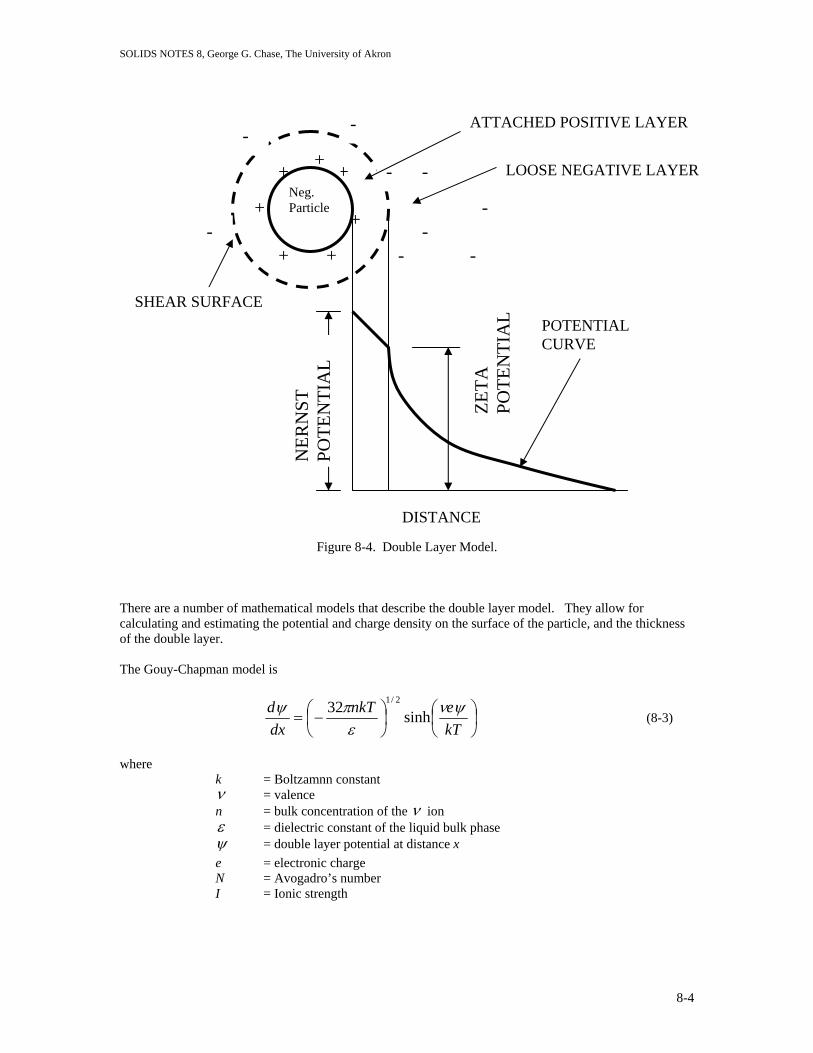
SOLIDS NOTES 8, George G. Chase, The University of Akron
Figure 8-4. Double Layer Model.
-
-
+
+
+ +
+
+ +
-
-
-
- -
-
- Neg. Particle
ATTACHED POSITIVE LAYER
LOOSE NEGATIVE LAYER
POTENTIAL CURVE
ZETA
PO
TEN
TIA
L
NER
NST
PO
TEN
TIA
L SHEAR SURFACE
DISTANCE
There are a number of mathematical models that describe the double layer model. They allow for calculating and estimating the potential and charge density on the surface of the particle, and the thickness of the double layer. The Gouy-Chapman model is
⎟⎠⎞
⎜⎝⎛
⎟⎠⎞
⎜⎝⎛−=
kTenkT
dxd ψν
επψ sinh32 2/1
(8-3)
where
k = Boltzamnn constant ν = valence n = bulk concentration of the ν ion ε = dielectric constant of the liquid bulk phase ψ = double layer potential at distance x e = electronic charge N = Avogadro’s number I = Ionic strength
8-4

SOLIDS NOTES 8, George G. Chase, The University of Akron
Integration of Eq.(8-3) gives ( )xχ−Ψ=Ψ exp0 (8-4) where χ is the Debeye-Huckel function
RT
INeε
πχ10008 22
= (8-5)
The potential approaches zero (becomes small enough that it is essentially zero) at x ≈ 3/χ. For small colloid particles of low charge, and in presence of electrolyte, the thickness of the double layer, d, is approximately 1/χ. For water
I
cmxd9103.2 −
≅ (8-6)
Hence, we see that the thickness is inversely proportional to the square root of the ionic strength. Some example values are listed in Table 8-1.
Table 8-1. Examples of Double layer Thickness
Medium d=1/χ, µm Distilled water 900 10-4M NaCl 31 10-4M MgSO4 15 Sea Water 0.4
A practical result of this is that the smaller the double layer thickness the closer the particles may come together and consequently are easier to coagulate. The addition of electrolyte (as long as it does not absorb on the surface) will reduce the double layer thickness.
8-5

SOLIDS NOTES 8, George G. Chase, The University of Akron
8.2.3 The Rate of Aggregation The rate of aggregation (i.e., coagulation) depends upon the rate of collisions between particles and the probability that collided particles will stick together. If, with pretreatment of electrolyte, electrical repulsion forces are absent, then aggregation depends upon the motion of the particles to collide.
Perikinetic Coagulation – coagulation due to Brownian motion Brownian motion alone has too low a collision rate (theory not presented here). Hence, it will not produce flocs of suitable size (1 mm) within a reasonable time.
Orthokinetic Coagulation – coagulation due to stirring and agitation Orthokinetic coagulation occurs when velocity gradients exist within the system (Figure 8-5).
Particles moving with the fluid Velocity
Velocity Profile
Figure 8-5. The relative velocities of particles bring the particles together so that they can coagulate.
Mixing and agitating devices can be divided into 4 groups. Paddles (stirred tanks) Baffles (in pipes, channels, or tanks) Pipes (wall affects, static mixers) Particles (packed or fluidized beds, bubble swarms, differential settling Various handbooks are available for sizing and designing such equipment. One obvious limitation to orthokinetic coagulation is if the velocity gradient becomes too large it can actually break up the flocs.
8-6

SOLIDS NOTES 8, George G. Chase, The University of Akron
Paddle Coagulation For the paddle wheel design the power is given by TOTAL
AREA
∑= AAp
(8-7) where CD= Drag Coefficient Ap = Projected paddle area of all paddles (Vp-V) ≈ (0.8) ⟨Vp⟩ Figure 8-6. Paddle Wheel Stirrer. Vp = Mean paddle speed The Mean Velocity Gradient is given by (8-8) The rule of thumb for effective coagulation is 20 s-1 < G < 75 s-1.
Paddle Example Calculate the mean velocity gradient for a 4- blade paddle in a 100 m3 tank of water at 20°C. ρ = 1 × 10³ kg/m3 CD = 1.2 (assumed) µ = 1.0 × 10⁻³ kg/ms Vp = (1 m)(2π)(4 rpm)(8 min/60 s) = 0.419 m/s Then
Which is adequate for the design. Figure 8-7. Example Paddle Wheel Stirrer.
n
( ) ( )VVAVV
ppp −×
−
A A
r
=
×=×=
2
C
Velocity ForceTime Distance/ ForcePower
2Dρ
Drag Force Relative velocity between paddle
and fluid
( )( ) ⎟⎠⎞
⎜⎝⎛==
sec60min2r rn rpmVp π
4rpm
3 m
0.5 m
1 m
( )µV
AVV
G
ppD
2
Mixture ofViscosity x VolumePower
3−
=
ρC=
( )( ) (( )( )
)
ssmkgm
mmsmmkgG
/36//101002
35.04/33.0/102.133
322
=
××= −
8-7

SOLIDS NOTES 8, George G. Chase, The University of Akron
Pipe Coagulators In straight horizontal pipes, the pressure loss is given by
fhP
=∆
ρ (8-9)
where c
f gV
DLfh
24
2
= (8-10)
f = Friction factor L = Pipe length D = Diameter gc = gravity constant
The mean velocity gradient is given by
µLA
PgQityvisxvolume
powerG c∆==
cos (8-11)
Substituting in Eqs.(8-9) and (8-10) gives
µD
fVG32
= (8-12)
In this geometry the criterion for G is 104 < G t < 105 for coagulation where t=L/V is the fluid residence time. Packed Bed Coagulation Steep velocity gradients are possible in packed beds. For spherical particles and low Reynolds number,
, the Ergun Equation, Eq.(4-25) in Chapter 4 simplifies to the Carman-Kozeny equation as 1≤eR
cp gd
VLP
32
20 )1(180ε
εµ −=
∆ (8-13)
and G becomes
µεAL
PgQxvolumefluid
powerG c∆==
viscosity
( ) 20
42
20
2 )1(56
)1(180εε
εε
pp dV
dV
G−
=−
= (8-14)
The same criterion for pipe flow applies here 104 < G t < 105 where the residence time is given by
0VL
rateflowvolumetricvolumeporet ε
== (8-15)
8-8

SOLIDS NOTES 8, George G. Chase, The University of Akron
Packed Bed Example: Calculate Gt and G for a fixed sand bed filter where
dp = 0.5 mm ε = 0.4 L = 0.6 m Vo = 5 m/hr
4
2
1004.6)/140)(432(
432/00139.0
6.0
/140/3600
/5)4.0(0005.0
)4.01(56
xssGt
ssm
mt
shrs
hrmm
G
==
==
=⎟⎠⎞
⎜⎝⎛−
= G is a relatively high value so large flocs will not form. However, this is appropriate because large flocs could clog the sand bed. Gt is in the design range criteria.
8.3 Zeta Potential A practical way to characterize the double layer is to measure its zeta potential. Several techniques are possible. One way is to measure the electro-phoretic effect. Electro-phoretic movement of small particles due to a voltage potential See website http://www.oxywave.com/nutrition/pdfs/zeta.pdf for more information on Zeta Potential.
Figure 8-8. Electrical field applied to a solution with particles. The particles migrate in the electrical field due to the strength of the field.
Commercial equipment are available (such as the Zeta Meter). The basic feature is to observe and measure the velocity of particles through a microscope. The observed velocity, VE, can be related to the zeta potential by
πµςε
4EVE = (8-16)
ε = dielectric constant of fluid E = external field ς = zeta potential
Changes in zeta potential ς can be observed when electrolyte is added as shown in Figure 7-4. The usual dosage for a useful coagulant in water is 100 to 400 mg/liter. A large number of salts such as Al2(SO4)3 and Na2P2O7 are available. Normally we want ς to be zero ( so that there is minimal repulsing force due to charge). There is a critical concentration, Cf, which is the concentration required of the salt to cause coagulation. Lists of Cf for electrolytes and solutions exist in literature.
8-9

SOLIDS NOTES 8, George G. Chase, The University of Akron
8.4 Flocculation by Polyelectrolytes The term flocculation is being used here to refer to the effects that polyelectrolytes (polymers) have on causing small particles to form large aggregates. One of the greatest advances in recent years in solid-liquid separation has been the development of polymers with remarkable properties to flocculate solutions when added only in trace quantities. Chemical Nature of Synthetic Polyelectrolytes Types of synthetic polymer flocculants fall into three categoreis: non-ionic (neutral) anionic (negative) cationic (positive) MONOMERS Acrylamide CH2=CH-CONH2
Sodium Acrylate CH2=CH-C-O- Na+
O O R1 Poly quaternary ester C-O-C2H4-N+ Cl- CH2=CH R2 R3 POLYMERS Non-Ionic Polyacrylamides (CH2-CH) CONH2 x Polyethyleneoxide (O-CH2-CH2) x Anionic Acrylamide (CH2-CH) (CH2-CH) Co-Polymer COOH x CONH2 y Polyacrylics (CH2-CH) COOH x Cationic Polyamines (CH2-CH2NH-CH2CH2NH) x
Notes: RNH2 Amino HC-C=O Carbonyl R-C-H Aldehydic
O C=C-H Vinylic CH2=CHCOOH Acrylic Acid (Reacts with base and GST sodium acrylate)
8-10

SOLIDS NOTES 8, George G. Chase, The University of Akron
Acrylamide (CH2-CH) (CH2-CH) Co-Polymers CONH2 x CH2
N+ Cl- CH3 CH3 CH3 y (CH2-CH) (CH2-CH) CONH2 x CO O- Na+ y The anionic/cationic character can be altered by co-polymerization of the various monomers. Any one product is characterized by
(1) Average molecular weight, and (2) Charge density distribution within the polymer molecule.
Molecular weights are classified as
High 20x106 Medium 10x106 Low 5x10⁶ Very Low <1x10⁶
More on chemistry of polyelectrolytes is given by W.L.K. Schwuyer, “Polyelectrolytes for Water and Waste Water Treatment”, CRC Press, Boca Raton, FL, 1981. Mode of Action and Application The mechanism of flocculation is charge neutralization and bridging.
+ + + + + + + + + + + +
+ +
+ +
+Increasing Ionic Strength
Figure 8-9. Positively charged polymers wrapping around negatively charged particles to form flocs.
8-11

SOLIDS NOTES 8, George G. Chase, The University of Akron
The best choice of polyelectrolyte is best maybe after laboratory trials of samples of the liquid to be clarified. Usually, for a given charge density, the polymer with the highest molecular weight will give the fastest sedimentation rate. Some practical points on efficient polyelectrolyte usage:
Add the polyelectrolyte to the main stream in a very dilute (<0.1%) solution Add as near as possible to the point where flocculation is required Add at points of local turbulence Add in stages at different points Add across whole stream to be treated Avoid turbulence after floc formation At high solids concentrations, add recycled or other dilution water to the system At low solids concentrations, recycle settled solids into the stream
8-12

SOLIDS NOTES 9, George G. Chase, The University of Akron
9. SEGREGATION Separation articles by size, density, or other material properties occurs when concentrations of one type of particle in a hopper or pile is much greater than the average for the entire mass. The process of separating the particles into different relative concentrations is referred to as segregation is the opposite. Segregation processes are the opposite of mixing processes, which in the latter the particles are blended into relatively uniform consistency.
Segregation is important in handling of powders because in many operations you want to avoid concentrations of one particle type or another.
9.1 Mechanisms We need to understand the mechanisms that cause segregation before we can design systems to minimize the effect. Differences in size, density, shape and resilience all contribute to segregation. By far, particle size difference is the most important parameter.
Four primary mechanisms cause segregation:
• TRAJECTORY SEGREGATION. When a powder cloud is in flight, groups of fine particles can travel farther than single large particles. For coarse particles, the larger particles tend to travel the farthest.
• PERCOLATION OF FINES (also called sifting). If a mass of particles is disturbed (by stirring, shaking, vibrating) such that the individual particles move relative to each other, a rearrangement in the packing occurs.
If a powder has a size distribution, it is easier for smaller particles to move into the void spaces between larger particles during the disturbance. Hence, in a storage hopper there is a tendency for small particles to migrate downward in the direction of gravity. A very small size difference is sometimes sufficient to cause a measurable segregation.
Segregation upon pouring a powder into a pile occurs frequently due to the percolation (as well as trajectory) mechanisms (Figure 9-1).
Figure 9-1. Segregation of particles when poured into a
HIGHER CONCENTRATIONIN LARGER PARTICLES
HIGHER CONCENTRATIONIN SMALLER PARTICLES
pile due to percolation.
9-1

SOLIDS NOTES 9, George G. Chase, The University of Akron
• RISE OF COARSE PARTICLES UPON VIBRATION. This effect can be demonstrated by submerging a large steel ball bearing in sand in a beaker. Upon vibrating the beaker the ball bearing rises to the top of the sand. This occurs even when the larger particle is much denser than the fine particles.
• ELUTRIATION SEGREGATION (also called fluidization). When a powder is discharged from a hopper, or is poured into the top of a hopper, a large volume of air is displaced. The air velocity may exceed the terminal velocity of the smaller particles. This can cause the fines to suspend while the coarse particles settle out.
The fines eventually settle on top of the suspension and form a layer on top of the powder that is concentrated in the fines.
9.2 Reduction in Segregation Methods to reduce segregation are aimed at reducing the effects that cause segregation.
• Make sizes of components as close as possible to the same size.
• Reduce the absolute size of the particles. Usually segregation is not a problem for particles smaller than about 30 microns for particle densities in the 2000 to 3000 kg/m3 range. For more dense particles the size must be smaller than 30 microns.
For very small particles the surface forces act to minimize the segregation effect on individual particles. However, if the surface forces cause the particles to agglomerate into larger particles, then segregation may become a problem again.
• A small amount of liquid may be added to a powder to increase its attractive forces between particles and minimize fines migration.
• Avoid situations that promote segregation
o Avoid pouring where the powder forms a sloping surface,
o Avoid pouring into the core of a hopper,
o Avoid vibrations, shaking, stirring (unless done to promote mixing),
o Use mass flow hoppers.
• Use continuous mixing.
• Use materials with large aspect ratios. Fibers and flakes do not segregate as easily as spherical shapes. Rough surfaces also reduce the segregation effect.
9-2

SOLIDS NOTES 9, George G. Chase, The University of Akron
9.3 Example A transport truck is loaded with a well mixed powder with a wide size distribution. The truck delivers the product to a facility 20 miles from the its loading point.
Is the material likely to segregate?
Yes, due to vibrations from the transport.
What material will exit first? Last?
Fines are more likely to exit first and coarse to exit last.
What options do you have to minimize the segregation at the delivery site?
Additives to reduce segregation (liquid? Fibers?)
Do the mixing at the delivery site.
Change the particle size mixture at the supply site to a more uniform size.
9-3

SOLIDS NOTES 10, George G. Chase, The University of Akron
10. HOPPER DESIGN People have stored powdered materials for thousands of years, at least as far back as man has harvested and stored crops. Prior to the 1960s storage bins were designed largely by guessing. This was all changed by the research of Andrew W. Jenike in the 1960s. His work identified the criteria that affect material flow in storage vessels. Jenike developed the theory and methods to apply the theory, including the equations and measurement of the necessary material properties. His primary works are published in "Gravity Flow of Bulk Solids", Bulletin 108, University of Utah Engineering Experiment Station, October 1961, and Bulletin 123, November 1964.*
Hoppers are used in industry for protection and storage of powdered materials. Hoppers must be designed such that they are easy to load. More importantly, hoppers must be designed such that they are easy to unload.
The way the hopper is designed affects the rate of flow of the powder out of the hopper, if it flows at all. Also, the way the hopper is designed affects how much of the stored material can discharge and whether there mixing of solid sizes or dead space that reduces the effective holding capacity of the hopper. These issues and others discussed here are important to consider when designing storage hoppers.
10.1 Flow Modes There are two primary and distinct types of flow of solids in hoppers, mass flow and funnel flow. There is also a special case that is a combination of these two flows called expanded flow. These flows get their names from the way in which solids move in the hoppers. The characteristics and differences between the flows are depicted in Figure 10-1.
The primary difference between mass and funnel flow is that in mass flow all of the material in the bin is in motion, though not necessarily all with the same velocity. In funnel flow only a core of material in the center above the hopper outlet is in motion while material next to the walls is stationary (stagnant).
Hoppers come in a variety of shapes and designs, not just conical. Figure 10-2 shows some of the more common designs found for mass flow hoppers. Also, a variety of designs are possible for funnel flow hoppers, shown in Figure 10-3.
* Other references that give a good summary on this topic include:
1. J. Bridgwater and A.M. Scott, “Flow of Solids in Bunkers,” in Handbook of Fluids in Motion, N.P. Cheremisinoff and R. Gupta eds., Butterworth, Ann Arbor, chapter 31, 807-846, 1983.
2. R. Holdich, Fundamentals of Particle Technology, Midland, Loughborough, UK, 2002.
3. M. Rhodes, Principles of Powder Technology, Wiley, New York, 1990.
10-1

SOLIDS NOTES 10, George G. Chase, The University of Akron
(B) FUNNEL FLOW
ACTIVE FLOWCHANNEL
STAGNANTREGION
MINIMUM LEVELFOR MASS FLOWIN HOPPER IS0.75 TO 1 x D
(A) MASS FLOW
D
FLOW
(C) EXPANDED FLOW
MASS FLOW
FUNNEL
Figure 10-1. In mass flow (A) all material moves in the bin including near the walls. In funnel flow (B) the material moves in a central core with stagnant material near the walls. Expanded flow (C) is a combination of mass flow in the hopper exit and funnel flow in the bin above the hopper (normally used in retrofit situations).
β Dp
L
p
(E) WEDGE (F) PYRAMID
(A) CONICAL HOPPER
Da
(B) SQUARE OPENING
β
(C) CHISEL
Figure 10-2. Common designs for mass flow hoppers.
10-2

SOLIDS NOTES 10, George G. Chase, The University of Akron
D
(A) PYRAMID,SQUARE OPENING
p Dc(B) CONICAL (D) CYLINDRICAL
FLAT-BOTTOMEDCIRCULAR OPENIN
(C) CYLINDRICALFLAT-BOTTOMEDSLOT OPENING
Dc
Figure 10-3. Common designs for funnel flow hoppers.
10.2 Hopper Design Problems Hopper design problems are normally one of two types; either the material does not discharge adequately from the opening in the hopper or the material segregates during the flow. The problems that we would like to solve or avoid are
• RATHOLING/PIPING. Ratholing or piping occurs when the core of the hopper discharges (as in funnel flow) but the stagnant sides are stable enough to remain in place without flowing, leaving a hole down through the center of the solids stored in the bin (See Figure 10-4a).
• FLOW IS TOO SLOW. The material does not exit from the hopper fast enough to feed follow on processes.
• NO FLOW DUE TO ARCHING OR DOMING. The material is cohesive enough that the particles form arch bridges or domes that hold overburden material in place and stop the flow completely (Figure 10-4b).
• FLUSHING. Flushing occurs when the material is not cohesive enough to form a stable dome, but strong enough that the material discharge rate slows down while air tries to penetrate into the packed material to loosen up some of the material. The resulting effect is a sluggish flow of solids as the air penetrates in a short distance freeing a layer of material and the process starts over with the air penetrating into the freshly exposed surface of material (Figure 10-4c).
• INCOMPLETE EMPTYING. Dead spaces in the bin can prevent a bin from complete discharge of the material.
10-3
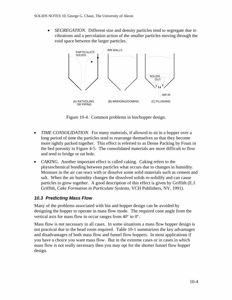
SOLIDS NOTES 10, George G. Chase, The University of Akron
• SEGREGATION. Different size and density particles tend to segregate due to vibrations and a percolation action of the smaller particles moving through the void space between the larger particles.
(B) BRIDGING/DOMING(A) RATHOLING OR PIPING
PARTICULATESOLIDS
BIN WALLS
SOLIDS
AIR IN
(C) FLUSHING
OUT
Figure 10-4. Common problems in bin/hopper design.
• TIME CONSOLIDATION. For many materials, if allowed to sit in a hopper over a long period of time the particles tend to rearrange themselves so that they become more tightly packed together. This effect is referred to as Dense Packing by Foust in the bed porosity in Figure 4-5. The consolidated materials are more difficult to flow and tend to bridge or rat hole.
• CAKING. Another important effect is called caking. Caking refers to the physiochemical bonding between particles what occurs due to changes in humidity. Moisture in the air can react with or dissolve some solid materials such as cement and salt. When the air humidity changes the dissolved solids re-solidify and can cause particles to grow together. A good description of this effect is given by Griffith (E.J. Griffith, Cake Formation in Particulate Systems, VCH Publishers, NY, 1991).
10.3 Predicting Mass Flow Many of the problems associated with bin and hopper design can be avoided by designing the hopper to operate in mass flow mode. The required cone angle from the vertical axis for mass flow to occur ranges from 40° to 0°.
Mass flow is not necessary in all cases. In some situations a mass flow hopper design is not practical due to the head room required. Table 10-1 summarizes the key advantages and disadvantages of both mass flow and funnel flow hoppers. In most applications if you have a choice you want mass flow. But in the extreme cases or in cases in which mass flow is not really necessary then you may opt for the shorter funnel flow hopper design.
10-4

SOLIDS NOTES 10, George G. Chase, The University of Akron
Table 10-1. Advantages and Disadvantages of Mass and Funnel Flow Hoppers
MASS FLOW FUNNEL FLOW
ADVANTAGES • Flow is more consistent • Reduced radial segregation • Stresses on walls are more
predictable • Effective use of full bin
capacity • First-in = First-out
• Low head room required
DISADVANTAGES • More wear of wall surfaces • Higher stresses on the
walls • More head room required
• Rat holing • Segregation • First-in = Last-out • Time consolidation effects
can be severe • Poor distribution of
stresses on walls may cause silo collapse
• Flooding • Reduction of effective
storage capacity.
10.3.1 BINDING MECHANISMS There are a number of mechanisms that cause solid materials to bind together and thus make flow difficult if not impossible. Some of these have been mentioned above.
Binding mechanisms include:
1. Solids Bridge (ie. Caking)
• Mineral Bridges • Chemical reactions • Partial melting • Binder hardening • Crystallization of dissolved substances
2. Adhesion and Cohesion
• There are a number of effects that are lumped together and are termed adhesion and cohesion. These include mechanically deformable particles that can plastically deform and bind to each other or with bin walls. Usually, very small particles display adhesion properties.
3. Interfacial forces.
10-5

SOLIDS NOTES 10, George G. Chase, The University of Akron
• Interfacial forces include liquid bridges and capillary forces between particles. These effects are due the contact surfaces between three phases (solid, liquid and gas) and interfacial tensions.
4. Attractive forces.
• Attractive forces include intermolecular forces such as van der Waal’s force, as well as longer range electrostatic and magnetic forces. There are also short range repulsive forces, but if the particles are in close enough contact the attractive forces are stronger.
5. Interlocking forces.
• Interlocking forces are due to the geometric entanglement that occurs with fibrous materials, analogous to what happens when you store coat hangers in a box - they become entangled.
Many earlier bin designs were based upon the angle of repose (see Chapter 4). However, the angle of repose alone is not sufficient to account for all of the mechanisms affecting hopper performance. The angle of repose is only useful in determining the contour of a pile, and its popularity among engineers is not due to its usefulness but due to the ease with which it can be measured.
10.3.2 TESTING REQUIREMENTS To design storage hoppers, the following material properties are needed:
• Internal friction coefficient • Wall friction coefficient • Permeability • Compressibility
Other factors that should be considered include temperature and moisture content along with phase diagrams if caking may be a problem.
One of the more common test apparatus is the Jenike Shear Tester. The Jenike Shear Tester has similarity to the Triaxial shear tester mentioned in Chapter 4. The powder sample is placed in a sample holder. The movement of the sample holder causes shear between a powder sample and a sample of the hopper wall as in Figure 10-5(a) to determine the wall friction coefficient. Or, the movement causes a shear internally in the powder sample as in Figure 10-5(b) to determine the internal coefficient of friction.
10-6

SOLIDS NOTES 10, George G. Chase, The University of Akron
COVERAPPLIED WEIGHT(NORMAL FORCE)
BRACKET
SAMPLE WALL MATERIAL
RING
POWDER SAMPLE
SHEAR FORCE
SHEAR FORCE
(a) Wall Friction Test. The powder sample is in contact with a wall sample. Shearing occurs between the powder and wall samples.
COVERAPPLIED WEIGHT(NORMAL FORCE)
BRACKET
RING
POWDER SAMPLE
SHEAR FORCE
SHEAR FORCE
(b) Internal Friction Test. The powder sample is sheared within itself.
Figure 10-5. Internal and wall friction tests with the Janike Shear Tester.
The friction tests are simple application of physics to determine the friction coefficients as discussed in Chapter 4 where the shearing force is related to the normal force N by the coefficient of friction
Fµ in the equation
F N= µ (10-1)
As commonly practiced, the coefficient of friction is expressed as the “angle” of wall friction given by φ as
φ µ= arctan( ) . (10-2)
Other shear test devices are available commercially, such as the rotating disk test called Peschl Tester, developed by I.A.S.Z. Peschl of The Netherlands, which operates by placing a sample between two circular disks and rotating the disks about their center axis relative to one another. This has an advantage over the Jenike Shear tester because the
10-7

SOLIDS NOTES 10, George G. Chase, The University of Akron
shearing can occur for longer periods of time, giving the particles opportunity to compact. However friction between the moving parts of the sample holder can cause doubt about the accuracy of the measured results and there are some doubts about the assumed zero stress at the center of the rotating disks.
Another test that has been around for many years is the annular shear cell. As with the rotating disk tester, the annular shear cell has infinite travel. The sample is placed in the annular space between two cylinders. A cover is placed on top of the sample to hold the powder in the annular space and to apply the desired normal force. The cover is rotated relative to the rest of the assembly, causing shearing of the sample. This device is good for elastic materials and for pastes. The measured results have not been fully tested for use in bin design and sealing powders can be a problem.
10.3.3 STRESSES IN HOPPERS AND SILOS Consider the equilibrium of forces acting on a differential element, , in a straight sided cylindrical silo (Figure 10-6). In the stationary situation the surrounding fluid (air) pressure acts uniformly on all solid particles throughout the silo.
dz
However, there are compressive normal stresses, , acting on the cross sectional area, A, due to the overburden of material above the volume element. There are also shear stresses,
Pv
τ R , of the solid phase acting on the silo walls. We list the various components contributing to the force in the z-direction:
zD z
z + dz
z
vv dPP +
vP
Overburden normal stress acting downward on the surface at z
P Av
Normal stress acting upward on the surface at
z z+ ∆
( )− +P dP Av v
Shear stress acting on the silo walls acting upward
− τ πR D dz
Gravity force acting downward on the differential element
ρ o Adz g
Rτ
Figure 10-6. Differential force balance on a cylindrical storage bin.
10-8

SOLIDS NOTES 10, George G. Chase, The University of Akron
At steady state (no accelerations, or neglecting inertial terms) the sum of the forces must equal zero. This gives the balance of forces as
( ) ( )A P A P dP Ddz Adz gv v v Ro− + − + =τ π ρ 0 (10-3)
which reduces to
(10-4) ( )− − +A dP Ddz Adz gv Roτ π ρ 0=
From physics we relate the shear stress at the wall to the lateral normal stress acting in the radial direction at the wall, , with the coefficient of friction, Pw µ ,
τ µR P= w
=
v
(10-5)
Substitution of Eq.(10-5) into (10-4) gives
(10-6) ( )− − +A dP P Ddz Adz gv woµ π ρ 0
which has both and terms. Pw Pv
Janssen solved this equation (H.A. Janssen, Versuche über Getreidedruck in Silozellen, Verein Deutcher Ingenieure, Zeitschrift, 39, August 1985, 1045-1049) by assuming that the vertical normal stress is proportional to the lateral normal stress (section 4.2.3), where
. (10-7) P KPw =
Substituting Eq. (10-7) into (10-6) and rearranging, where AD
=π 2
4, we get
dPK
DP
gDK
dzv v
o
= − −⎛⎝⎜
⎞⎠⎟
44
µ ρµ
. (10-8)
Equation (10-8) is integrated with the boundary condition that Pv = 0 at , to obtain z = 0
PgDKg
KzDv
o
c= − −
⎛⎝⎜
⎞⎠⎟
⎛⎝⎜
⎞⎠⎟
ρµ
µ4
14
exp . (10-9)
where the is the gravity constant conversion factor to convert the result from units of mass to units of force. This latter expression is known as the Janssen Equation. When we plot the pressure in the silo as a function of depth from the free surface of the granular material at the top we get a plot as shown in Figure 10-7.
gc
10-9

SOLIDS NOTES 10, George G. Chase, The University of Akron
PRESSURE
zHYDROSTATIC
BULK SOLIDS
Figure 10-7. Vertical normal stress profile in a silo.
Note that in Figure 10-7 the asymptotic pressure for large depth is only a function of the silo diameter and not on depth. This is one reason why commercial silos are designed tall and narrow rather than short and squat.
At the bottom of the silo is the converging hopper section. Andrew Jenike (A.W. Jenike, Storage and Flow of Solids, Bulletin No. 123, Utah Engineering Experiment Station, University of Utah, Salt Lake City, Utah, 1964) postulated that the magnitude of stress in the converging section is proportional to the distance from the hopper apex (as well as a dependence on the angle). The stress is written as
. (10-10) as indicated in Figure 10-8.
(σ σ θ= r, )
θ
σr
HOPPER OPENING
Figure 10-8. The stress, σ , in the hopper is a function of position ),( θr .
10-10
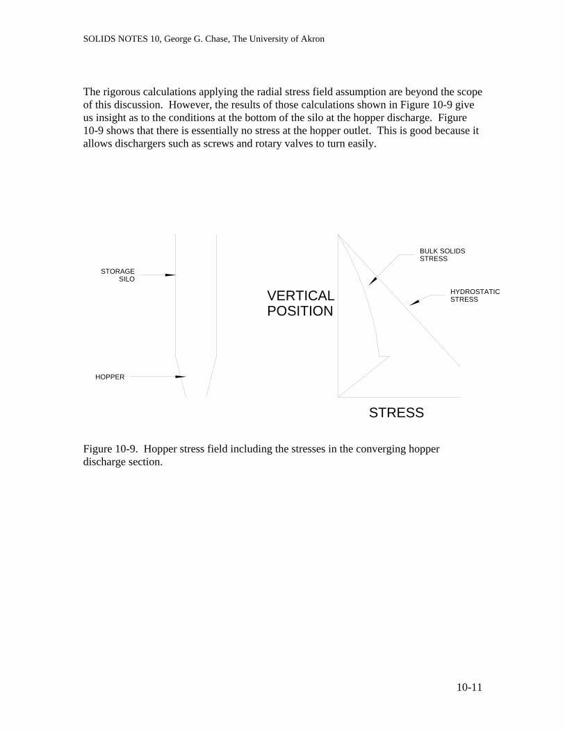
SOLIDS NOTES 10, George G. Chase, The University of Akron
The rigorous calculations applying the radial stress field assumption are beyond the scope of this discussion. However, the results of those calculations shown in Figure 10-9 give us insight as to the conditions at the bottom of the silo at the hopper discharge. Figure 10-9 shows that there is essentially no stress at the hopper outlet. This is good because it allows dischargers such as screws and rotary valves to turn easily.
STORAGESILO
HOPPER
STRESS
VERTICALPOSITION
HYDROSTATICSTRESS
BULK SOLIDSSTRESS
Figure 10-9. Hopper stress field including the stresses in the converging hopper discharge section.
10-11
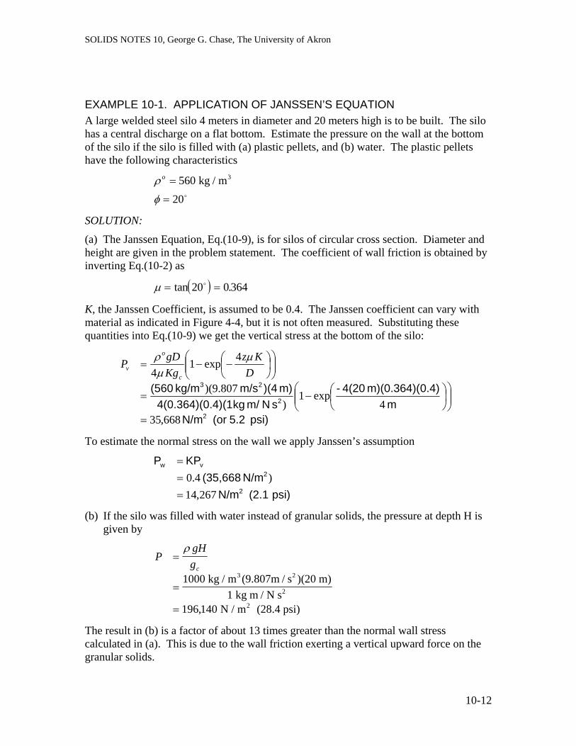
SOLIDS NOTES 10, George G. Chase, The University of Akron
EXAMPLE 10-1. APPLICATION OF JANSSEN’S EQUATION A large welded steel silo 4 meters in diameter and 20 meters high is to be built. The silo has a central discharge on a flat bottom. Estimate the pressure on the wall at the bottom of the silo if the silo is filled with (a) plastic pellets, and (b) water. The plastic pellets have the following characteristics
ρ
φ
o =
=
56020
kg / m3
o
SOLUTION:
(a) The Janssen Equation, Eq.(10-9), is for silos of circular cross section. Diameter and height are given in the problem statement. The coefficient of wall friction is obtained by inverting Eq.(10-2) as
( )µ = =tan .20 0 364o
K, the Janssen Coefficient, is assumed to be 0.4. The Janssen coefficient can vary with material as indicated in Figure 4-4, but it is not often measured. Substituting these quantities into Eq.(10-9) we get the vertical stress at the bottom of the silo:
psi) 5.2 (or N/m m
0.4)m)(0.364)( 4(20-s Nm/ kg .4)(14(0.364)(0
m) )(4m/s kg/m (560
2
2
23
668,354
exp1)
807.9)(
4exp14
=
⎟⎟⎠
⎞⎜⎜⎝
⎛⎟⎠⎞
⎜⎝⎛−=
⎟⎟⎠
⎞⎜⎜⎝
⎛⎟⎠⎞
⎜⎝⎛−−=
DKz
KggDP
c
o
vµ
µρ
To estimate the normal stress on the wall we apply Janssen’s assumption
psi) (2.1 N/m
N/m (35,668 KPP
2
2vw
267,14)4.0
===
(b) If the silo was filled with water instead of granular solids, the pressure at depth H is given by
PgHgc
=
=
=
ρ
1000 kg / m (9.807m / s )(20 m)1 kg m / N s
N / m (28.4 psi)
3 2
2
2196 140,
The result in (b) is a factor of about 13 times greater than the normal wall stress calculated in (a). This is due to the wall friction exerting a vertical upward force on the granular solids.
10-12

SOLIDS NOTES 10, George G. Chase, The University of Akron
10.3.4 HOPPER ANGLE AND OUTLET SIZE FOR MASS FL0W HOPPERS To size and design a hopper we determine the design necessary for mass flow operation based upon the material properties. The properties that are used in the design of a mass flow hopper are the effective angle of internal friction, the material flow function, and the angle of wall friction between the powder material and the wall material.
In a mass flow hopper during discharge the stress distribution is such that a stable arch or funnel flow do not occur and therefore the flow will not stop. This analysis can be used in the design of a new hopper or to check the suitability of an existing hopper for use with a particular material.
10.3.4.1 The Material Flow Function Whether a hopper operates in mass flow or funnel flow depends on the flow properties of the powder material and how it interacts with the hopper walls. One way of analyzing stresses in a solid is through Mohr Circles. Mohr circles relate shear stress to the normal stress.
Given normal and shear stresses on a solid block (Figure 10-10), it is possible to find an angle (θ ) of a surface within the block such that the normal stress on the new surface is a maximum (or minimum) and the shear forces are zero.
xxσ
Figure 10-10. Stresses on a block. (a) Angle θ is a surface with maximum/minimum normal force with zero shear. (b) Triangle shows maximum and minimum normal forces with no shear. (c) Mohr Circle.
θ
yxσ
xyσ
yyσ
yxσ
xxσ
Normal
Max
Min
Shear
(b)
SHEA
R S
TRES
S A
XIS
NORMAL AXIS
MAX NORMAL
MIN NORMAL
MOHR
CIRCLE
(c)
yyσ
xyσ
(a)
10-13

SOLIDS NOTES 10, George G. Chase, The University of Akron
Similarly, we can find an angle at which the shear stress is a maximum or minimum. Usually this occurs 90° from the maximum normal stress. The maximum and minimums are plotted on the stress plot (Figure 10-10 (c)).
For powder flow in a hopper, we want to know the shear stress needed to initiate flow (overcome the coefficient of static friction). A material’s flowability depends upon the shear strength and how the shear strength changes with compacting stresses.
In experiments on a shear tester you must pre-stress the sample by applying a maximum load (critical point on the Jeniky Yield Locus (JYL) curve) and then reducing the applied stress during the experiments (Figure 10-11). Several different maximum loads are applied to generate at least three different JYL curves.
• If the material is cohesive, the JYL is not a straight line and does not pass through the origin. When extrapolated down to the zero shear stress the JYL crosses perpendicular to the Normal Stress axis.
• The JYL represents a surface that divides between operating conditions. Above the JYL the shear stress is sufficient to cause powder movement. Below the JYL the normal stress is too large for the powder to flow at the give shear stress.
JYL
Critical Point
(End Point) Shea
r Stre
ss
Normal Stress
Figure 10-11. Jeniky Yield Locus (JYL) curve plotted from experimental data of Shear Stress versus Normal Stress for a given starting Critical Point.
10-14

SOLIDS NOTES 10, George G. Chase, The University of Akron
Several Mohr Circles may be drawn that are tangent to the JYL. We are interested in two in particular.
1. The Mohr Circle passing through the origin and tangent to the JYL represents the stress needed to initiate flow in an arch (ie, to cause the arch to collapse) (Figure 10-12). The diameter of this Mohr Circle is the Unconfined Yield Stress (UYS),
. cf
Shea
r Stre
ss
Normal Stress
cf
JYL
Figure 10-12. Mohr Circle passing through origin and tangent to the JYL. This is used to determine the value of , the Unconfined Yield Stress (UYS). cf
10-15

SOLIDS NOTES 10, George G. Chase, The University of Akron
2. The Mohr Circle passing through the critical point (end point) represents the state of the material at the compacting stress (Figure 10-13).
This represents the conditions for failure without volume change.
We assume it represents the stress conditions of the powder as it flows downward towards the outlet.
Normal Stress
Mohr circle
Intersects Critical Point and is tangent to the JYL
1σ
JYL
Critical Point
(End Point)
Shea
r Stre
ss
Figure 10-13. Mohr Circle passing through the critical point and tangent to the JYL. This is used to determine the value of 1σ .
Each JYL gives an and cf 1σ . The versus cf 1σ data are plotted to obtain the Material Flow Function (MFF) (Figure 10-14). The MFF curve represents the stress needed to make an arch collapse as a function of the compacting stress under which it was formed. Stresses below the MFF and the arch is stable. For points above the MFF the material is flowing and the frictional analysis in deriving the MFF does not apply.
10-16

SOLIDS NOTES 10, George G. Chase, The University of Akron
MFF
Non-cohesive
Less cohesive
More cohesive
cf
1σ
Figure 10-14. The Material Flow Function. More cohesive materials have larger values. Non-cohesive materials have small values.
cf
cf
10.3.4.2 The Effective Angle of Internal Friction The effective angle of internal friction, δ , is determined from the JYL plot. δ is the angle of the slope of the line through the origin that is tangent to the Mohr Circles at the critical point, as shown in Figure 10-15.
Figure 10-15. The angle δ is the angle of the tangent line to the Mohr Circles at the critical points that passes through the origin.
Normal Stress
Shea
r Stre
ss
Critical Points
δ
Multiple JYL curves
10-17

SOLIDS NOTES 10, George G. Chase, The University of Akron
10.3.4.3 The Angle of Wall Friction The last property needed is the wall friction, wφ , between the powder and the wall of the hopper. This property is determined from experiments run with the shear tester as shown in Figure 10-5(a) where the measured shear force is plotted versus to the normal load (Figure 10-16). Often the data are linear. If they are nonlinear then the smallest angle is used.
wδ
Shea
r Stre
ss
Normal Stress
Figure 10-16. Plot to determine the wall angle, wδ .
10.3.4.4 Determining the Minimum Hopper Outlet Size The forces acting on the powdered material stored in a hopper tend to (1) compact the powder (i.e., reduce its bulk density), and (2) the shear stresses in the material tend to make it flow. Jenike (A.W. Jenike, Storage and Flow of Solids, Bulletin No. 123, Utah Engineering Experiment Station, University of Utah, Salt Lake City, Utah, 1964) showed that for an element at any position inside of a mass flow hopper, the ratio of the compacting stress to the shear stress has a constant value that he called the flow factor:
AS
ff 1
stressshear appliedstress compacting= factor, flow σ
= (10-11)
Jenike published charts from which ff is determined. Charts for symmetrical slot outlet hoppers and for conical hoppers are shown in Figures 10-17 and 10-18.
10-18

SOLIDS NOTES 10, George G. Chase, The University of Akron
0
10
20
30
40
50
0 10 20 30 40 50 60 70
Semi-included angle, degrees
Wal
l Fric
tion,
deg
rees
1
1.1
1.2
1.3
1.4
1.5
1.6
1.7
1.8
1.9
2
δ=30
δ=40
δ=60
δ=50δ=60
δ=40
δ=30
δ=50
δ=60
δ=50
δ=45
δ=40
δ=35
δ=30
Flow
Fac
tor,
ff
Flow Factor Curves
Wall Friction Curves
Figure 10-17. Design chart for symmetrical slot outlet hoppers. For example (dashed arrows), and gives and o22=wφ
o50=δ o5.30=θ 19.1=ff .
10-19

SOLIDS NOTES 10, George G. Chase, The University of Akron
0
10
20
30
40
0 5 10 15 20 25 30 35 40 45
Semi-included angle, degrees
Wal
l Fric
tion,
deg
rees
1
1.1
1.2
1.3
1.4
1.5
1.6
1.7
1.8
1.9
2
δ=30
δ=40
δ=60
δ=50
δ=60
δ=40δ=30
δ=50
δ=60
δ=50
δ=40
δ=35
δ=30
Flow
Fac
tor,
ff
Flow Factor Curves
Wall Friction Curves
Figure 10-18. Design chart for conical outlet hoppers. For example, and gives and
o22=wφo50=δ o5.20=θ 29.1=ff .
10-20

SOLIDS NOTES 10, George G. Chase, The University of Akron
The intersection of the MFF curve in Figure 10-14 with the line through the origin having a slope of 1/ff is the Critical Applied Stress (CAS) (Figure 10-19). Recall that the condition of flow (no arching) occurs for points on or above the MFF curve. Therefore the hopper should operate where the 1/ff curve is above the MFF curve, ie, above or to the right of the CAS.
MFF
1/ff curve
CAS
Unconfined
Yield Stress, cf
or
Applied Stress, AS
1σ
Figure 10-19. Intersection of the 1/ff and MFF curves defines the Critical Applied Stress (CAS).
The stress in the outlet of the hopper may drop below the CAS if the opening is too small. Hence, the outlet opening size must ensure that the applied stress exceeds the CAS. Correlations relating the outlet size to the CAS are provided.
θ
D
Semi included angle
For conical hoppers, Figure 10-20, the opening diameter, , is given by D
co ggCASHD
/)(ρ
θ= (10-12)
602)( θθ +=H (10-13)
Where θ is in degrees, from the charts in Figures 10-17 or 10-18. Typical values for H are about 2.4. Figure 10-20. Conical Hopper with
outlet size D and semi included angle θ .
10-21

SOLIDS NOTES 10, George G. Chase, The University of Akron
W
L
For symmetrical slot outlet hoppers the opening size is determined from
co ggCASHW
/)(ρ
θ= (10-14)
1801)( θθ +=H (10-15)
Figure 10-21. Symmetrical slot ohopper of opening size W x L.
utlet WL 3> (10-16)
These are the minimum dimensions for the outlets to ensure mass flow. In the next section some correlations are given for estimating the flow throughput of the solids through the opening. Larger openings may be used for greater throughput and still maintain mass flow. In practical design the angle θ is reduced by as a margin of safety.
o3
EXAMPLE 10-2. EXAMPLE HOPPER DESIGN The Shear Stress – Yield Stress JYL plots for a certain material yield the data in Table 10-2. Determine the wall slope and opening size to ensure mass flow in a conical hopper for this material. Assume the bulk density is 1300 kg/m3.
Table 10-2. Experimental Shear Stress data on example powder.
Shear Stress Internal Friction JYL Curve number (Figures 10-12 and 10-13)
1σ(kPa)
cf (kPa)
1 2.4 0.97 2 2.0 0.91 3 1.6 0.85 4 1.3 0.78
Wall Friction Measurements (Figure 10-16)
Normal Force (kPa)
Shear Force (kPa)
1 2.0 0.689 2 3.0 1.03
Effective Angle of Internal Friction, δ (Figure 10-15)
Rise, y∆ (kPa)
Run, x∆ (kPa)
Data taken from tangent line to Mohr Circle at critical point
1.0 1.73
10-22
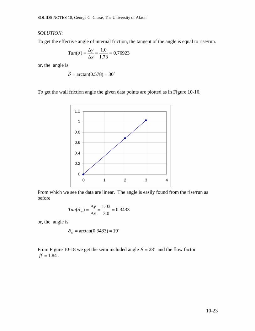
SOLIDS NOTES 10, George G. Chase, The University of Akron
SOLUTION:
To get the effective angle of internal friction, the tangent of the angle is equal to rise/run.
76923.073.10.1)( ==
∆∆
=xyTan δ
or, the angle is o30)578.0arctan( ==δ
To get the wall friction angle the given data points are plotted as in Figure 10-16.
0
0.2
0.4
0.6
0.8
1
1.2
0 1 2 3 4
From which we see the data are linear. The angle is easily found from the rise/run as before
3433.00.3
03.1)( ==∆∆
=xyTan wδ
or, the angle is o19)3433.0arctan( ==wδ
From Figure 10-18 we get the semi included angle and the flow factor .
o28=θ84.1=ff
10-23

SOLIDS NOTES 10, George G. Chase, The University of Akron
The vs cf 1σ data are plotted to obtain the Material Flow Function (MFF), and the ff value is used to plot the 1/ff curve as in Figure 10-19, to obtain the CAS value
00.20.40.60.8
11.21.4
0 1 2 3
Stre
ss,
fc
σ1
CAS
Hence, the CAS = 0.83 kPa.
From Eq. 10-13
H = 2.47
From Eq.10-12
( )m
sNmkg
smmkgPamNkPaPakPaD
161.0
1/807.9/1300
)//1)(/1000)(83.0(47.2 223
2
=
⋅=
Hence, for a mass flow conical hopper the minimum diameter of the opening is 0.161 m. As a margin of safety, the semi included angle is reduced by 3 degrees and the hopper design angle is 24 degrees.
10-24

SOLIDS NOTES 10, George G. Chase, The University of Akron
10.4 Rate of Discharge from Hoppers There are a number of methods for calculating discharge rates from silos or hoppers. A few of the equations are provided here.
10.4.1 COARSE PARTICLES
For coarse particles (particles > 500 microns in diameter) there are two equations commonly used, one for mass flow and one for funnel flow
MASS FLOW – JOHANSON EQUATION
The Johanson equation, derived from fundamental principles (Trans. Min. Engrs. AIME, 232, 69-80, (1965); Trans. ASME, 224-230 (1966) is
)()1(2 θρ
TanmBgAm o
+=& (10-17)
where θ = semi included angle of the hopper
m& = discharge rate (kg/sec) oρ = bulk density (kg/m3)
g = gravity acceleration (9.807 m/s2)
Depending on whether a conical or symmetric slot opening hopper the remaining parameters in the equation are given in Table 10-3.
Table 10-3. Parameters in the Johanson Equation, Eq.(10-18)
Parameter Conical hopper Symmetric slot hopper
B D, diameter of outlet W
A 2
4Dπ WL
m 1 0
FUNNEL FLOW – BEVERLOO EQUATION
A theoretical expression for funnel flow discharge is not available. Beverloo (W.A. Beverloo, H.A. Leniger, J. van de Velde, The Flow of Granular Solids Through Orifices, Chem Eng Sci, 115, 260-269, 1961) tested a variety of seeds and derived an empirical equation. The Beverloo Equation is
5.25.0 )(58.0 po kdDgm −= ρ& (10-18)
where dp = particle diameter (m)
10-25

SOLIDS NOTES 10, George G. Chase, The University of Akron
k = constant, typically 1.3 < k < 2.9 with k = 1.4 if not discharge rate data are available. The term accounts for the wall effect where the particles do not fully flow at the perimeter of the outlet.
pkd
D = outlet diameter (m). For non-circular outlets the hydraulic diameter is used
)perimeteroutlet ()area sectional cross(4
=D
The remaining parameters are defined as in Eq.(10-17).
10.4.2 FINE PARTICLES
Fine particles (dp < 500 microns) tend to flow slower by a factor of 100 to 1000 than that predicted by the Johanson equation. The reason for this is the effect of air drag on the motion of the particles is much greater for fine particles.
Particle beds need to dilate (increase distance between particles) before the powder can flow. This means air must penetrate into the bed through the bottom surface of the hopper as the powder moves through the constriction formed by the conical walls. For fine particles the pore diameters in the powder bed are small and there is a significant amount of air drag that resists the powder motion.
Carleton gives an expression for predicting the velocity of the solids as (Powder Tech., 6, 91-96, 1972)
gd
VB
V
pp
oo =+3
5
34
32
312
15sin4
ρ
µρθ (10-19)
oo AVm ρ=&
where = average velocity of solids discharging (m/s) oV
A, B = given in Table 10-3
µρ , = air density and viscosity
pρ = particle density
oρ = bulk density of the powder bed
The remaining parameters are defined with Equations (10-17) and (10-18).
10-26

HANDOUT 10-1
xxσ
θ
xyσ
yxσ
xyσ
yyσ
yxσ
xxσ
(a)
(b)
Normal
Shear
Min
Max
yyσ
MAX NORMAL
NORMAL AXIS
SHEA
R S
TRES
S A
XIS
MIN NORMAL
MOHR CIRCLE
(c)

HANDOUT 10-2
Normal Stress Sh
ear S
tress
Critical Point (End Point)
Normal Stress
Shea
r Stre
ss
cf
Normal Stress
Critical Point (End Point)
1σ
JYL
Shea
r Stre
ss
JYL
JYL

HANDOUT 10-3
Normal Stress
Shea
r Stre
ss
Critical Points
δ
MFF
Non-cohesive
Less cohesive
More cohesive
Multiple JYL curves
cf
1σ

HANDOUT 10-4
0
10
20
30
40
50
0 10 20 30 40 50 60 70
Semi-included angle, degrees
Wal
l Fric
tion,
deg
rees
1
1.1
1.2
1.3
1.4
1.5
1.6
1.7
1.8
1.9
2
δ=30
δ=40
δ=60
δ=50δ=60
δ=40
δ=30
δ=50
δ=60
δ=50
δ=45
δ=40
δ=35
δ=30
Flow
Fac
tor,
ff
Flow Factor Curves
Wall Friction Curves
Figure 10-17. Design chart for symmetrical slot outlet hoppers. For example (dashed arrows),
and gives and
o22=wφo50=δ o5.30=θ 19.1=ff .
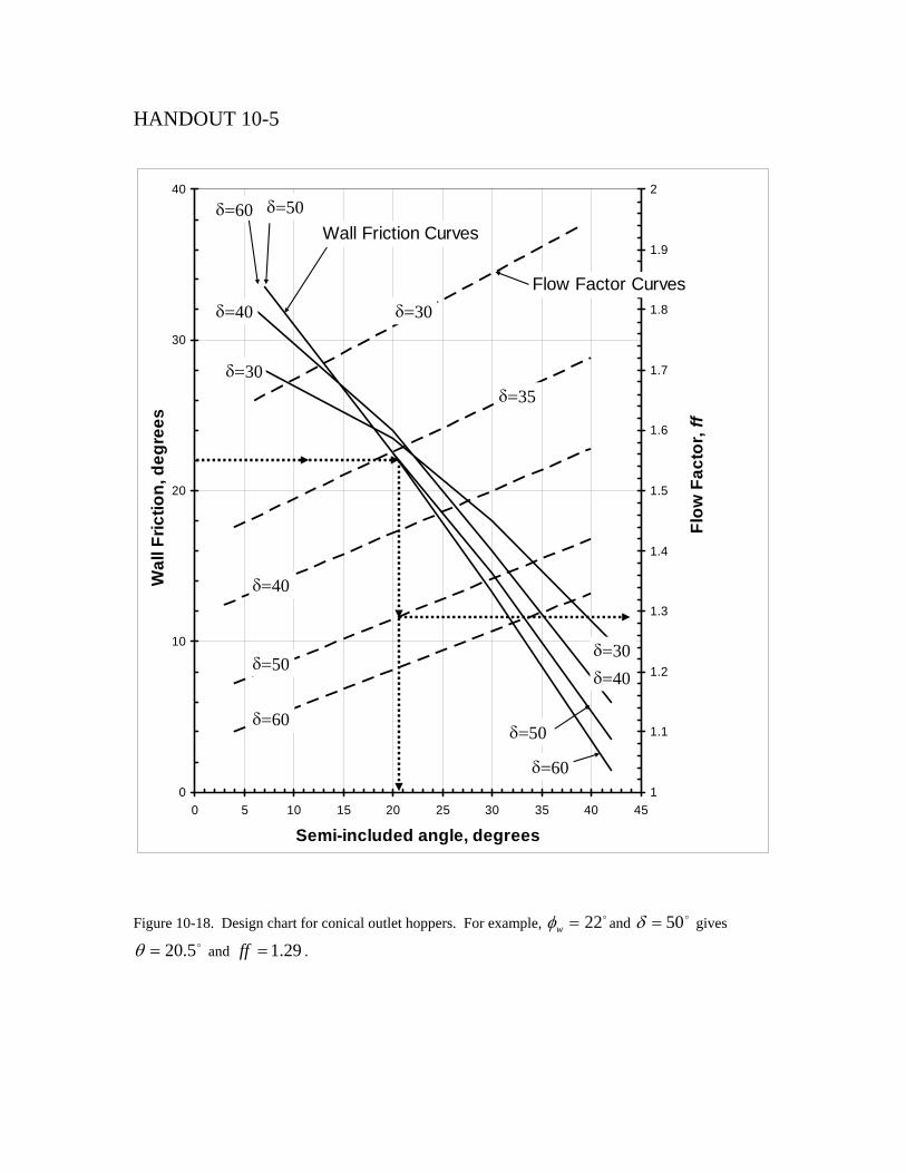
HANDOUT 10-5
0
10
20
30
40
0 5 10 15 20 25 30 35 40 45
Semi-included angle, degrees
Wal
l Fric
tion,
deg
rees
1
1.1
1.2
1.3
1.4
1.5
1.6
1.7
1.8
1.9
2
δ=30
δ=40
δ=60
δ=50
δ=60
δ=40δ=30
δ=50
δ=60
δ=50
δ=40
δ=35
δ=30
Flow
Fac
tor,
ff
Flow Factor Curves
Wall Friction Curves
Figure 10-18. Design chart for conical outlet hoppers. For example, and gives
and .
o22=wφo50=δ
o5.20=θ 29.1=ff

HANDOUT 10-6 Steps on using the shear stress data to design a hopper.
1. Rotating Shear Test Plot SHEAR STRESS vs NORMAL STRESS
Internal Friction Get fc vs σ1
Get δ
δ
SHEAR STRESS
fc σ1 NORMAL STRESS
JYL
2. Rotating Shear Test Wall material
Get φw
3. Fit φw and δ to hopper correlation
Get θ and ff. (θ is the theoretical angle of the hopper; in final design subtract 3 degrees for margin of safety)
4. Plot 1/ff on mff curve (fc vs σ1) to get CAS
Get CAS
5. Use CAS and θ in correlations to select opening size.
SHEARSTRESS
NORMAL STRESS
φw
δ
δ
wφ
ff
θ
fc
MFF CAS
Slope 1/ff
σ1

HANDOUT 10-7
D
θ Semi included angle
For conical hoppers, Figure 10-20, the opening diameter, , is given by D
co ggCASHD
/)(ρ
θ= (10-12)
602)( θθ +=H (10-13)
Where θ is in degrees, from the charts in Figures 10-17 or 10-18. Typical values for H are about 2.4.
Figure 10-20. Conical Hopper with outlet size D and semi included angle θ .
L
W
For symmetrical slot outlet hoppers the opening size is determined from
co ggCASHW
/)(ρ
θ= (10-14)
1801)( θθ +=H (10-15)
WL 3> (10-16) Figure 10-21. Symmetrical slot outlet h
of opening size W x L. opper

HANDOUT 10-8 10.4.1 COARSE PARTICLES (particles > 500 microns in diameter)
MASS FLOW – JOHANSON EQUATION
)()1(2 θρ
TanmBgAm o
+=& (10-17)
where θ = semi included angle of the hopper m& = discharge rate (kg/sec)
oρ = bulk density (kg/m3) g = gravity acceleration (9.807 m/s2)
Table 10-3. Parameters in the Johanson Equation, Eq.(10-18) Parameter Conical hopper Symmetric slot hopper
B D, diameter of outlet W
A 2
4Dπ
WL
m 1 0
FUNNEL FLOW – BEVERLOO EQUATION
5.25.0 )(58.0 p
o kdDgm −= ρ& (10-18) where dp = particle diameter (m)
k = constant, typically 1.3 < k < 2.9 with k = 1.4 if not discharge rate data are available.
)perimeteroutlet ()area sectional cross(4
=D
10.4.2 FINE PARTICLES (dp < 500 microns)
CARLETON EQUATION
gd
VB
V
pp
oo =+3
5
34
32
312
15sin4
ρ
µρθ (10-19)
oo AVm ρ=&
where = average velocity of solids discharging (m/s) oVA, B = given in Table 10-3
µρ, = air density and viscosity
pρ = particle density oρ = bulk density of the powder bed

SOLIDS NOTES 11, George G. Chase, The University of Akron
11. GRADE EFFICIENCY Classification is the art of separating solid particles in a mixture of solids and fluid into fractions according to particle size or density by methods other than screening. Most methods of separation are not 100% effective. There is usually a range of particle sizes that are separated with varying degrees of efficiency. The variation in the efficiency is referred to as the Grade Efficiency Curve. A good discussion on Grade Efficiency is given by Svarovsky.1
The grade efficiency is a way of characterizing how well particles are separated according to size (density, or some other desired property). Separation of particles by size is referred to as classification.
The process of classification has been used for many years. Some methods make a sloppy separation while others make a sharp classification. Usually for the same production rate, the sharp separation will be more expensive, as could be deduced from the 2nd Law of Thermodynamics.
11.1 Why Do We Classify Particles? We classify particles to remove contaminants and unlike particles (wheat from chaff, or metal particles from polymers). We classify to remove unwanted parts of a size distribution. In Figure 11-1 indicates the tailings and oversize particles that may be removed from a material for a particular purpose.
FREQUENCY
SIZE
TAILINGS OVERSIZE
Figure 11-1. Size distribution indicating undesired tailings and oversize particle ranges.
1 Ladislav Svarovsky, Solid-Liquid Separation, 3rd ed., Butterworths, London, 1990, Chapter 3.
11-1

SOLIDS NOTES 11, George G. Chase, The University of Akron
There are many processes that may be used to classify particles:
Screening
Sieving
These methods are effective, but rate of production may be low.
Air or water classification These methods take advantage of different drag forces acting on different size particles.
Physical separations
• Magnetic • Gravity • Electrostatic • Radiation • Color
These methods rely on physical properties other than differences in fluid drag to classify.
An example of gravity separation if a mixture of plastic milk jugs (high density poly ethylene, density of 0.95 g/cc) and plastic ware (polystyrene, density of 1.05 g/cc) is dumped into a tank of water, the milk jug plastic will float while the plastic ware will sink. This provides a simple means for separation. Some additional examples of separators are given in Figures 11-2 through 11-4.
r
Solid Trash Feed Stream
r Paper Exit Stream
Figure 11-2. Air classifier for separating large drag force to gravitational force ratiopaper to separate from plastics and metals
Plastic and metals input
Figure 11-3. Example of a magnetized seroller the ferrous materials cling longer toseparation.
Ai
Plasticmetals
Metals anPlastics EStream
paper and l of the air
.
parator. As the belt tha
Air
Ai
and input
d xit
ow density materials from solid waste streams. The on the low density materials causes materials such as
Magnetized cylinder
t
Rotating belPlastic and non-ferrous metals output
Ferrous metals output
the belt rotates around the magnetized cylindrical n non-ferrous materials fall off and thus allow
11-2

SOLIDS NOTES 11, George G. Chase, The University of Akron
sw
Fmcin
1Sop
Tosh
T
Wme
2 CT
Top Vie
t
t
Monolayer of Chopped plastic
Laser scan to ID colors by location
Air jets use puffs of air to blow plastic squares into separate bins
w
Side Vies
igure 11-4. Separation by color. Chopped plastic pieces are spread in a monolayer on a poving belt. Lasers scan the belt and identify the locations of plastic pieces of specific col
orresponding to the locations of the identified plastic pieces apply puffs of air to blow the to bins.
0.2 Measuring Efficiency eparation efficiency is directly related to processing costs. Most separations are not 100%utlet streams of the separation may be concentrated in the desired or undesired products, bure. The challenge is to determine the best way to define and measure the efficiency of th
he method of separation considered here is called the Grade Efficiency (For an alternativen thermodynamic entropy, see the paper by Guistino et.al.2). A black box powder separatiown in Figure 11-5. The total mass balance gives
. fc MMM +=
he total separation efficiency, , is defined as TE
M
MMME fc
T −== 1 .
e assume that there is no agglomeration or communition in the separator. For a particle sasses of size x in each stream are noted by . By analogy with Eq.(11-2),
fficiency of separation of size x is defined as cxfxx MMM ,,
x
cxx M
MG =
JM Giustino, G.G. Chase, and M.S. Willis, “Thermodynamic Separation Efficiency and Sriteria for Multiphase Processes: A Comparison of Rigorous and Approximate Models,” Sechnology, 5 (3), 153-164, 1995.
Air Hole
Moving Bel
Moving Bel
Air Jet
erforated ors. Air jets plastic pieces
efficient. The ut may not be e separation.
method based on process is
(11-1)
(11-2)
ize, x, the the grade
(11-3)
edimentation eparations
11-3

SOLIDS NOTES 11, George G. Chase, The University of Akron
Fines Stream Total mass Mf of powder
Coarse Stream Total mass Mc of powder
Black box Separation Process
Feed Stream Total mass M of powder
Figure 11-5. Black box (hypothetical) separation process to separation coarse particles from fine particles.
We know from the definitions of frequency distributions (see notes Section 3, Properties of Particulate Solids) that the mass and mass components of each stream are related by
(11-4)
x
x
x
dFMdxfM
MM
===
x)size of fraction(
similarly, cxccxccx dFMdxfMM == (11-5)
Hence, the grade efficiency is related to the size distribution functions by
x
cxc
MffMxG =)( . (11-6)
A typical plot of the grade efficiency versus the particle size is shown in Figure 11-5. The area under the curve plotted in Figure 11-6 represents the coarse cut (the stream with the larger particles) and the area above the plotted curve represents the fines cut. Svrovsky1 gives more detail on defining and measuring these curves.
1Fines Cut
Coarse Cut
)(xG
0
x
Figure 11-6. Typical S-shaped grade efficiency curve. At a point, x, on the curve, G(x) represents the fraction of particles of size x that are separated out of the feed stream and contained in the fines product stream.
11-4

SOLIDS NOTES 11, George G. Chase, The University of Akron
For a continuous steady process the curve in Figure 11-6 is steady. For an unsteady process such as filtration, the curve changes with time, as shown in Figure 11-7.
Increasing Time
Increasing Time
)(xG
)(xG
xCake Filtration
xDepth Filtration
Figure 11-7. Comparison of typical grade efficiency curves for Cake Filtration and Depth Filtration. In a typical cake filtration, as the filter cake depth increases, the cake itself improves the separation and the grade efficiency shifts with increasing efficiencies for smaller particles. In Depth filtration, initially the filter may perform very well. Gradually the capture sites in a typical depth filter are occupied (though other mechanisms such as straining may occur) and the fine particles start to bleed through. Hence in Depth Filtration the grade efficiency curve shifts toward larger particles as the filter becomes less efficient at capturing small particles.
As an example of how you might apply the grade efficiency curve, consider the water filter pumps used by backpackers on a hiking trail. One of the objectives of the filter is to remove harmful bacteria from water. Bacteria are typically greater than 1 micron in size. If you have the choice of two filters with grade efficiency curves shown in Figure 11-8, the savy backpacker would choose filter A because it is better than 99.99% effective at removing 1 micron particles. Filter B appears to be only about 50% effective at removing 1 micron particles.
1 10
AB
x, microns
)(xG
Figure 11-8. Comparison of grade efficiency curves for two filters, A and B. Filter A is approximately 99+% efficient at removing 1 micron particles. Filter B is only about 50% efficient at removing 1 micron particles, though it is 99+% efficient at removing 10 micron particles.
11-5

SOLIDS NOTES 11, George G. Chase, The University of Akron
One of the reasons for inventing the Grade Efficiency is that it makes some calculations regarding the separation of particles by size easier. Consider an arbitrary process in Figure 11-9a, where the amount of material of size x entering the process is given by Mx and the amount of material of size x leaving in the coarse and fine streams are given by
(11-7) xxcx MGM =
(11-8) ( ) xxcx MGM −= 1
You can use the grade efficiency to determine the amounts of material of size x in various streams of processes that are cascaded in series or parallel. For example, in Figure 11-9b the streams exiting process 2 have amounts of size x given by
(11-9) xxxxc MGGM 122 =
( ) xxxxf MGGM 122 1−= (11-10)
Suppose Mc2x is your product in stream C2 in Figure 11-9b. The amount of product in stream C1 is Mc1x = G1xMx as given by Eq.(11-7). Because G < 1, then Mc2x < Mc1x. This can be generalized to conclude that the more separations steps in your process the smaller the yield of your product.
Mcx G(x)
Mx
Mfx
a. Arbitrary process that divides the feed stream M into fines and coarse streams. The grade efficiency of this process is given by G.
Mc2x
C1
C2 2 G2x 1
G1x
Mx Mf2x
Mf1x
b. Two arbitrary process in series with grade efficiencies G1 and G2 .
Figure 11-9. One and Two arbitrary processes in series with corresponding Grade Efficiencies.
11-6

SOLIDS NOTES 11, George G. Chase, The University of Akron
11-7
11.3 Cut Size and Sharpness of Cut To compare efficiencies between steady state processes, we define cut size and sharpness of cut. Normally, cut size refers to the 50% cut size, denoted . This is the particle size for which 50% of the particles exit the separation process in the coarse product stream and 50% exit in the fines product stream.
50x
Sharpness of cut is defined as a ratio of particle sizes specified at two efficiencies, typically at 20% and 80%. The sharpness of cut is defined as
20
8020/80 x
xI = (11-11)
By this definition, and because the grade efficiency is a monotonically increasing curve, the sharpness must be greater than or equal to unity. In an idealized case in which there is a perfect separation, where all particles less than the 50% cut size exit in the fines stream and all particles greater than the cut size exit in the coarse stream, the sharpness of cut equals unity. Real separation processes have a sharpness of cut greater than unity. These concepts are shown in Figure 11-10.
Idealized sharp cutoff
with 120
80 =xx
)(xG
x x
)(xG
80
50
20
50
x20 x50 x80 x50
The sharper the cut the smaller the triangular areas between the real and idealized grade efficiency curves.
(a) (b)
Figure 11-10. (a)Typical grade efficiency curve with the particle sizes indicated for which the separation is 20, 50, and 80 percent efficient. (b) The idealized sharp cutoff grade efficiency curve is a vertical line
Other definitions of sharpness of cut are also used, including
1. 80
2080/20 x
xI = which is the inverse of . x values such as 90/10 could also be defined. 20/80I
2. Variance in the slope, dxdG
.
3. Slope of the grade efficiency curve, dx
xdGI x)(
=
4. Sum of triangular areas in Figure 11-10(b).

SOLIDS NOTES 11, George G. Chase, The University of Akron
11.4 Construction of the Grade Efficiency Curve In the ideal case you would feed into your separator a material with a monodispersed particle size distribution (of size x).
You would
• Measure , , , xM cxM fxM
• Calculated , )(xG
• Repeat for other size x (until you have enough points to construct your curve or you loose patience).
This approach is not very realistic because of the difficulty in obtaining monodispersed materials (especially in the very small particle size range) and because of the time and effort required.
In real applications you need to measure two of the following
• Feed rate,
• Coarse product rate,
• Fines product rate,
and you need at least two of the following,
• Feed particle size distribution,
• Coarse particle size distribution,
• Fine particle size distribution.
It is best to have data from the smaller of the two product streams because errors in sampling are smaller than when you subtract two larger streams to get the smaller stream. As indicated in Figure 11-11, the flow rate of the smaller stream may be less than the error of measurement of the larger streams.
10 lbm/hr ± ?
10,000 lbm/hr ± 50 lbm/hr
9,990 lbm/hr ± 50 lbm/hr
Figure 11-11. Example in which the size of the smaller product stream is smaller than the error in measurements of the other two steams. Due to the error, it is better to measure the smaller stream directly instead of calculating it from the two larger streams.
11-8

SOLIDS NOTES 11, George G. Chase, The University of Akron
11.5 Example 1 A sample of the feed, coarse, and fines streams for a separation of a material "Hexamethyl chicken wire" is screened with the following results:
Screen Size (microns)
Average Particle Size
Feed Size mass Fraction retained on screen
xF∆
Mass Rate of particles size x in Feed Stream
xM
Coarse Size mass Fraction retained on screen
cxF∆
Mass Rate of particles size x in Coarse Stream
cxM
Fines Size mass Fraction retained on screen
fxF∆
Mass Rate of particles size x in Fines Stream
fxM
( )x
cx
MM
xG =
850 ~0 ~0 ~0
600 725 0.30 0.45 0.075
425 512.5 0.40 0.45 0.325
300 362.5 0.20 0.09 0.365
212 256 0.10 0.01 0.235
Total 1 1 1
The stream rates are:
0
0.1
0.2
0.3
0.4
0.5
0.6
0.7
0.8
0.9
1
0 100 200 300 400 500 600 700 800 900 1000
Size, microns
G(x
)
• Feed rate = 100 lbm/hr
• Coarse Product Rate = 60 lbm/hr
• Fines Product Rate = 40 lbm/hr
Plot the grade efficiency curve and calculate I20/80.
11-9

SOLIDS NOTES 11, George G. Chase, The University of Akron
SOLUTION
A sample of the feed, coarse, and fines streams for a separation of a material "Hexamethyl chicken wire" is screened with the following results:
Screen Size (microns)
Average Particle Size
Feed Size mass Fraction retained on screen
xF∆
Mass Rate of particles size x in Feed Stream
xM
Coarse Size mass Fraction retained on screen
cxF∆
Mass Rate of particles size x in Coarse Stream
cxM
Fines Size mass Fraction retained on screen
fxF∆
Mass Rate of particles size x in Fines Stream
fxM
( )x
cx
MM
xG =
850 ~0 0 ~0 0 ~0 0 1
600 725 0.30 30 0.45 27 0.075 3 0.9
425 512.5 0.40 40 0.45 27 0.325 13 0.68
300 362.5 0.20 20 0.09 5.4 0.365 14.6 0.27
212 256 0.10 10 0.01 0.6 0.235 9.4 0.06
Total 1 100 1 60 1 40
The stream rates are:
• Feed rate = 100 lbm/hr
• Coarse Product Rate = 60 lbm/hr
• Fines Product Rate = 40 lbm/hr
Plot the grade efficiency curve and calculate I20/80.
0
0.1
0.2
0.3
0.4
0.5
0.6
0.7
0.8
0.9
1
0 100 200 300 0 500 00 700 800 900 1000
G(x
)
BLANK FORM FOR CALCULATING GRADE EFFICIENCY
SOLUTION:
Recall that xx FMM ∆=
cxccx FMM ∆=
fxffx FMM ∆=
Using these equations and a basis of 1 hour, the table is filled in.
The calculated points for the Grade Efficiency are plotted on the graph and a curve is fitted to the points. From the curve the , , and values are estimated to be 330, 450, and 625 microns respectively.
20x 50x 80x
The sharpness of cut is calculated to be
Note, mass retained on the 850 micron screen is zero. In the limit Gx approaches 1 at this size (Gx = 1 at the size for which all particles exit the separator in the Coarse stream). Plot Gx vs the Average particle size to determine the x20, x50, and x80 values.
. 528.0625330
80/20 ==I
20x 50x 80x
40 Size, mic6
rons
11-10

SOLIDS NOTES 11, George G. Chase, The University of Akron
creen
s)
Average Feed Size
Mass f
Coarse ss
SSize (micron
Particle Size
mass Fraction retained on screen
xF∆
Rate oparticlessize x in Feed Stream
xM
Size maFraction retained on screen
cxF∆
Mass f
Fines Size
Rate oparticlessize x in Coarse Stream
cxM
mass Fraction retained on screen
fxF∆
Mass f
Rate oparticlessize x in Fines Stream
fxM
( )x
cx
MM
xG =
0
0.1
0.2
0.3
0.4
0.5
0.6
0.7
0.8
0.9
1
0 100 200 300 400 500 600 700 800 900 1000
Size, microns
G(x
)
he stream rates are:
ct Rate =
Plot the nd
T
• Feed rate =
• Coarse Produ
• Fines Product Rate =
grade efficiency curve acalculate I20/80.
11-11

SOLIDS NOTES 11, George G. Chase, The University of Akron
11.5 Example 2 The grade efficiency represents the fractional amount of particles by mass of size x in the feed stream that exits the separator in the coarse stream. Derive a formula in terms of Grade efficiencies for determining the fractional amount of particles of size x in the coarse stream exiting separator 2 in the compound process shown in Figure 11-12 where the grade efficiencies of both processes are the same (ie., G1x = G2x).
2 G2
1 G1
M feed Mc1 coarse
Mc2 coarse
Mf2 fines
Mf1 fines
SOLUTION
The fractional amount of size x in the coarse stream exiting separator 2 can by determined by
(the subscript ‘x’ is dropped from this notation, but is implied).
For an arbitrary process, from Eqs.(11-7) and (11-8)
and GMM c = ( )MGM f −= 1
Hence
and MGM c 11 = ( )MGM f 11 1−= (1)
For process 2
122 fc MGM = and ( ) 122 1 ff MGM −= (2)
where is the feed stream to process 2. 1fM
Hence, by combining equations (1) and (2) we get
( )( )MGGM f 122 11 −−=
Since G1 = G2 this expression simplifies to
( ) MGM f2
2 1−=
or
( )22 1 GM
M f −= .
11-12

HANDOUT 11-1
FREQUENCY
SIZE
TAILINGS OVERSIZE
Figure 11-1. Size distribution indicating undesired tailings and oversize particle ranges.
There are many processes that may be used to classify particles:
Screening
Sieving
These methods are effective, but rate of production may be low.
Air or water classification These methods take advantage of different drag forces acting on different size particles.
Physical separations
• Magnetic • Gravity • Electrostatic • Radiation • Color
These methods rely on physical properties other than differences in fluid drag to classify.
Paper Exit Stream
r
r
Solid Trash Feed Stream
Figure 11-2. Air classifier for separating large drag force to gravitational force ratiopaper to separate from plastics and metals
Ai
Metals anPlastics EStream
paper and l of the air
.
Air
Ai
d xit
ow density materials from solid waste streams. The on the low density materials causes materials such as
11-1

HANDOUT 11-2 Magnetized cylinder
t Plastic and metals input
Figure 11-3. Example of a magnetized separator. Asroller the ferrous materials cling longer to the belt thaseparation.
t
t
Monolayer of Chopped plastic
w
w
Figure 11-4. Separation by color. Chopped plastic pmoving belt. Lasers scan the belt and identify the loccorresponding to the locations of the identified plastiinto bins.
Rotating bel
Plastic and non-ferrous metals output
Ferrous metals output
the belt rotates around the magnetized cylindrical n non-ferrous materials fall off and thus allow
s
Top VieLaser scan to ID colors by location
Air jets use puffs of air to blow plastic squares into separate bins
Side Vie
s
ieces are spread in a monolayer on a pations of plastic pieces of specific col
c pieces apply puffs of air to blow the
Air Hole
Moving Bel
Moving Bel
Air Jet
erforated ors. Air jets plastic pieces
11-2

HANDOUT 11-3
Figure 11-5. Black box (hypothetical) separation process to separation coarse particles from fine particles.
Fines Stream Total mass Mf of powder
Coarse Stream Total mass Mc of powder
Black box Separation Process
Feed Stream Total mass M of powder
The total mass balance gives fc MMM += . (11-1)
The total separation efficiency, , is defined as TEM
MMME fc
T −== 1 . (11-2)
Assume that there is no agglomeration or comminution in the separator. For a particle size, x, the masses of size x in each stream are noted by . The cxfxx MMM ,, grade efficiency of separation of size x is defined as
x
cxx M
MG = (11-3)
(11-4)
x
x
x
dFMdxfM
MM
===
x)size of fraction(
For the Coarse Steam cxccxccx dFMdxfMM == (11-5)
Hence x
cxc
MffMxG =)( . (11-6)
1
Figure 11-6. Typical S-shaped grade efficiency curve. At a point, x, on the curve, G(x) represents the fraction of particles of size x that are separated out of the feed stream and contained in the fines product stream.
Fines Cut
Coarse Cut
x
)(xG
0
11-3

HANDOUT 11-4
A sample of the feed, coarse, and fines streams for a separation of a material "Hexamethyl chicken wire" is screened with the following results: Screen Size (microns)
Average Particle Size
Feed Size mass Fraction retained on screen
xF∆
Mass Rate of particles size x in Feed Stream
xM
Coarse Size mass Fraction retained on screen
cxF∆
Mass Rate of particles size x in Coarse Stream
cxM
Fines Size mass Fraction retained on screen
fxF∆
Mass Rate of particles size x in Fines Stream
fxM
( )x
cx
MM
xG =
850 ~0 ~0 ~0
600 725 0.30 0.45 0.075
425 512.5 0.40 0.45 0.325
300 362.5 0.20 0.09 0.365
212 256 0.10 0.01 0.235
Total 1 1 1
The stream rates are:
0
0.1
0.2
0.3
0.4
0.5
0.6
0.7
0.8
0.9
1
0 100 200 300 400 500 600 700 800 900 1000
Size, microns
G(x
)
• Feed rate = 100 lbm/hr
• Coarse Product Rate = 60 lbm/hr
• Fines Product Rate = 40 lbm/hr
Plot the grade efficiency curve and calculate I20/80.
11-4

SOLIDS NOTES 14, George G. Chase, The University of Akron
14. DUST EXPLOSIONS Historically dust explosions have occurred in processing plants where dry organic powdered are handled. Grain elevators (storing corn, rice, oats, soybeans, wheat, etc.) are well known for dust explosions, but other powdered materials can cause explosions as well. It is common knowledge that organic materials can burn. Most often the burning of organic materials does not cause an explosive force. What makes the powdered materials different that when burned they can cause an explosion? Powdered materials have very high surface areas per unit mass. When burned, a powdered material gives off product gases (CO2, H2O, etc.) at a rate in proportion to the surface area. When the powdered material is confined within a grain elevator or storage building the rapid release of product gases can create a significant gas pressure within the building. With the right conditions dust explosions can exceed 100 psi. Most buildings will collapse if the interior pressure exceeds about 10 psi (70 kPa). Reinforced concrete structures typically can withstand 2 – 8 psi of static pressure. The dryer and finer the dust, the more explosive is its nature. An acceptable minimum concentration of dust is 1.13 g/cm3; higher concentrations are considered dangerous. Dust explosions can occur within storage buildings, conveying systems, hoppers, sieves, etc. when the conditions are right. When a dust explosion occurs seven conditions are nearly always present:
1. Oxygen (air) 2. Fuel source (the dust itself) 3. Dust is mixed or suspended in air 4. The dust concentration exceeds a minimum needed for the explosive reaction 5. Ignition source 6. Dry dust 7. All of the elements are in a confined space
Removal of one or more of these conditions can prevent a dust explosion (elimination of three or more is preferred). Motion sensors, belt alignment sensors, heat sensors, and magnets are common safety devices used to prevent dust explosions. How are these devices used to prevent dust explosions?
• Motion sensors can be used to detect when machinery moves in ways that they are not designed (vibrations, friction, etc, that might cause sparks).
• Belts must be properly aligned otherwise the rubbing of belts can cause friction and the friction can cause heat that could be an ignition source.
• Heat sensors can alert operators to trouble spots so that heat sources can be eliminated before an explosion occurs.
• Magnets can remove iron and other metals that when conveyed in the powder can cause sparks.
By their nature, grain elevators and hoppers must handle dusts in concentrations greater than the minimum required. Proper designs of these devices include pressure relief panels that can blow away to reduce the pressure and prevent the explosion from damaging the whole building. Catastrophic explosions (destruction of a large building) usually occur due to secondary explosions. The secondary explosions occur in other locations in building when powders are suddenly suspended into the air because of the vibrations and shocks caused by the primary explosion (the first explosion in a grain elevator). Probably the most important prevention of secondary explosions is good housekeeping. Do not let powder to accumulate on floors, pipes, walkways, etc. Removal of these powders removes the fuel source for the secondary explosions.
14-1

SOLIDS NOTES 14, George G. Chase, The University of Akron
References
1. Bodurtha, F.T., Industrial Explosion Prevention and Protection, McGraw-Hill, NY, 1980.
2. Field, P. Dust Explosions, Elsevier, N.Y., 1982.
3. Bartknecht, W. Dust Explosions, Springer-Verlag, N.Y., 1989.
4. Eckhoff, R.K., Dust Explosions in the Process Industries, Butterworth, Rushden, United Kingdom, 1991.
5. Crowl, D.A. and Luvar, J.F., Chemical Process Safety: Fundamentals with Applications, Prentice
Hall, Englewood Cliffs, NJ, 1990.
14-2