Solar and Stellar Photospheric Abundances

Carlos Allende PrietoInstituto de Astrofısica de Canarias

C/ Vıa Lactea S/N, E-38200 La Laguna, Tenerife, Spainemail: callende@iac.es

http://hebe.as.utexas.edu

Abstract

The determination of photospheric abundances in late-type stars from spectroscopic obser-vations is a well-established field, built on solid theoretical foundations. Improving those foun-dations to refine the accuracy of the inferred abundances has proven challenging, but progresshas been made. In parallel, developments on instrumentation, chiefly regarding multi-objectspectroscopy, have been spectacular, and a number of projects are collecting large numbers ofobservations for stars across the Milky Way and nearby galaxies, promising important advancesin our understanding of galaxy formation and evolution. After providing a brief description ofthe basic physics and input data involved in the analysis of stellar spectra, a review is madeof the analysis steps, and the available tools to cope with large observational efforts. Thepaper closes with a quick overview of relevant ongoing and planned spectroscopic surveys, andhighlights of recent research on photospheric abundances.

1

arX

iv:1

602.

0112

1v1

[as

tro-

ph.S

R]

2 F

eb 2

016

Contents

1 Introduction 3

2 Physics 72.1 Model atmospheres . . . . . . . . . . . . . . . . . . . . . . . . . . . . . . . . . . . . 72.2 Line formation theory . . . . . . . . . . . . . . . . . . . . . . . . . . . . . . . . . . 9

2.2.1 Opacity: lines and continua . . . . . . . . . . . . . . . . . . . . . . . . . . . 102.2.2 Departures from LTE . . . . . . . . . . . . . . . . . . . . . . . . . . . . . . 11

3 Working Procedures 143.1 Obtaining stellar spectra and reference data . . . . . . . . . . . . . . . . . . . . . . 143.2 Atmospheric parameters . . . . . . . . . . . . . . . . . . . . . . . . . . . . . . . . . 153.3 Determining abundances from spectra . . . . . . . . . . . . . . . . . . . . . . . . . 173.4 Tools for abundance determination . . . . . . . . . . . . . . . . . . . . . . . . . . . 18

3.4.1 Interactive tools . . . . . . . . . . . . . . . . . . . . . . . . . . . . . . . . . 183.4.2 Automated tools . . . . . . . . . . . . . . . . . . . . . . . . . . . . . . . . . 19

4 Observations 204.1 Libraries . . . . . . . . . . . . . . . . . . . . . . . . . . . . . . . . . . . . . . . . . . 204.2 Ongoing projects . . . . . . . . . . . . . . . . . . . . . . . . . . . . . . . . . . . . . 204.3 In the future . . . . . . . . . . . . . . . . . . . . . . . . . . . . . . . . . . . . . . . 224.4 Examples of recent applications . . . . . . . . . . . . . . . . . . . . . . . . . . . . . 23

4.4.1 The Galactic disk . . . . . . . . . . . . . . . . . . . . . . . . . . . . . . . . . 234.4.2 Globular clusters . . . . . . . . . . . . . . . . . . . . . . . . . . . . . . . . . 234.4.3 The most metal-poor stars . . . . . . . . . . . . . . . . . . . . . . . . . . . 234.4.4 Solar analogs . . . . . . . . . . . . . . . . . . . . . . . . . . . . . . . . . . . 24

5 Reflections and Summary 24

2

1 Introduction

Stars drive the chemical evolution of the universe. Starting from hydrogen, stars build up heavierelements, first by nuclear fusion in their cores, and later by neutron bombardment in the finalstages of their lives. A fraction of the gas processed in stars makes it back to the interstellarmedium, where it can again collapse under gravity and form new stars, repeating the cycle.

This picture is complicated by the fact that the stellar-processed gas mixes with unpolluted (orless polluted) gas, diluting the metals1 available at any given location. Far from being a closed box,the Milky Way strips stars and gas from its immediate neighbors. Depending mainly on their mass,stars of different masses produce (and sometimes destroy) nuclei of different elements, but theirnucleosynthetic yields also depend on other parameters such as chemical composition. Most heavyelements are actually produced during the final stages of the lives of stars, in nuclear reactionsdriven by supernovae explosions. Mixing within stars blurs and modifies the radial stratificationpredicted by simple, spherically symmetric, models of stars. In addition, close binaries lead tofar more complex stellar evolution scenarios where the events expected for an isolated star mayhappen sooner, or never take place.

The formation and chemical evolution of the Galaxy is therefore closely entangled with theproblem of stellar structure and evolution, which includes energy production and nucleosynthesisin stars. Observationally, we see the progressive enrichment in metals of the Milky Way in thechemical compositions of intermediate and low-mass stars that were born at different times. Thechemical mixtures found in the surfaces of main-sequence stars, essentially undisturbed by thenuclear reactions going on deep in the interior, sample the chemistry of the gas in the interstellarmedium from which they formed. Stars preserve those samples for us to study.

Reading the chemical patterns frozen in the stellar surfaces involves solving a different problem,that of the structure of the outermost layers of a star. Part of the energy initially produced inthe nuclear reactions in the interior of a star escapes immediately in the form of neutrinos; thisamounts to ∼ 2% in the solar case. The rest diffuses outwards slowly, finally reaching the surfaceof the star where photons decouple from matter. The distribution of escaping photons reflects thestate of the gas in the stellar atmosphere. Conversely, the radiation field has a profound influenceon the physical structure of the atmosphere through its effect on the energy balance.

To model a stellar atmosphere we need to know how much energy flows through it, σT 4eff ,

where σ is the Stefan–Boltzmann constant, the surface gravity of the star, g = GM/R2, and itschemical composition. The observed spectrum constrains these parameters, but sometimes thereis additional information available. For example, if we know the parallax of a star and its angulardiameter, we can readily compute its radius.

Deep enough, the atmosphere is optically thick and Local Thermodynamic Equilibrium (LTE)holds, so that the radiation field is known directly from the gas temperature. As we move upwardsin the gravitationally stratified atmosphere, density decreases, photons travel longer distancesbetween their emission and reabsorption or scattering, and begin to escape, cooling the gas (seeFigure 1). Bound-bound transitions within discrete energy levels in atoms and molecules blockthe light at specific wavelengths, at which the increased opacity shifts the optical depth scaleoutwards, to cooler atmospheric layers, imprinting dark stripes, absorption lines, in the spectrum,as illustrated in Figure 2.

Absorption lines are easily seen at high spectral resolution, and constitute the main indicatorof the chemical composition of the gas in a stellar atmosphere. Of course, line strengths areheavily influenced by temperature, which dictates the relative populations of the energy levels,and somewhat by pressure, which has an impact on ionization and molecular equilibrium, andthrough collisional broadening. But for any given values of temperature and pressure, the strength

1 We talk about metals when referring to any element heavier than helium.

3

Figure 1: Relative LTE populations for three atomic levels of an atom with energies ∆E = 0, 1 and2 eV from the ground state (assuming the same level degeneracy) as a function of Rosseland opticaldepth (τ) in the solar atmosphere. The populations are arbitrarily normalized to be unity for theground level in the innermost layer shown. The color in the background indicates temperature,increasing from black (about 3000 K) to white (about 10 000 K). At the layers relevant for lineformation, typically −3 < log τ < 0, the populations of levels separated by 1 eV differ by a factorof about five.

of an unsaturated absorption line is proportional to the number of absorbers. This simple fact,allows us to determine the chemical composition of stars.

There is a favorite among the stars: the Sun. This is arguably the best-observed and best-understood star, and constitutes a perfect test bed for spectral analysis techniques. The comparisonof the Sun with other stars, and in particular, the derivation of accurate absolute fluxes is com-plicated by its large angular size, but otherwise it offers multiple advantages. We can resolve itssurface, determine the statistical properties of solar granulation, quantify limb darkening, or ex-amine the center-to-limb variation of spectral lines. With the exception of highly volatile elements(hydrogen, carbon, nitrogen, oxygen, and the noble gases), we can compare the derived abundancesaccessible from the solar spectrum with those in CI carbonaceous chondrites, which are thoughtto preserve the abundance proportions in the pre-solar nebula.

In the context of the solar system, solar photospheric abundances, having suffered little variationsince the formation of the pre-solar nebula,2 serve as a reference. In a stellar context, the Sun isbasically a calibrator for our models, both of model atmospheres as explained above, as well asmodels of stellar structure and evolution, which still have a number of tunable parameters. For

2 Over the solar birth, elements heavier than hydrogen are expected to be reduced at the solar surface by up to10% due to diffusion (Turcotte and Wimmer-Schweingruber, 2002).

4

Figure 2: A small section of a high resolution spectrum of the red giant Arcturus, the nearest giantat merely 11 pc from us. The strongest transitions in this spectral window are the Na i D doublet.

example, it is typically imposed that a one-solar mass model has the solar radius and luminosity at4.5 Gyr, the age of the Sun. In the context of the Galaxy, and galaxy evolution, solar abundancesset again a reference to anchor the rest of the abundances – it corresponds to the abundances inthe interstellar medium 4.5 Gyr ago at a distance from the Galactic center of about 8 kpc.

Abundances in the Sun can also be measured from emission lines formed in the upper atmo-sphere, where the temperature gradient reverses to reach millions of degrees in the solar corona,and from solar energetic particles ejected in flares, or from particles collected from the solar wind.Nevertheless, these measurements are subject to larger uncertainties than those typically involvedin the analysis of photospheric absorption lines. The additional sources of error are associated withour limited knowledge about the physical conditions in the upper solar atmosphere, required tointerpret measurements, or with distortions introduced before or in the process of performing themeasurements. In addition, a poorly-understood fractionation process related to the so-called firstionization potential (FIP) effect leads to elements with ionization energies lower than about 10 eVto appear more abundant in solar energetic particles and in the corona than in the underlyingphotosphere.

Despite that the Sun’s composition sets a reference for abundances elsewhere in the universe,there are still important gaps in our knowledge of the solar composition. Solar photosphericabundances are usually determined relative to hydrogen, given that the strength of spectral lines isproportional to the ratio of line and continuum opacity, and H− is the dominant source of continuumopacity for a solar-like star. Meteoritic abundances, in turn, need to be referred to other elements(usually silicon), as meteorites have no hydrogen left. After rescaling, the agreement between solarphotospheric abundances and CI chondrites abundances is better than 10% for most elements,

5

but there are notable exceptions: Sc, Co, Rb, Ag, Hf, W, and Pb show differences in excess of20%, and beyond the estimated uncertainties. In addition, there are some elements for whichthe photospheric values have associated significant uncertainties (Cl, Rh, In, Au, and Tl), andthe interesting case of Mg, where the estimated error bars appear slightly inconsistent with theobserved difference between the Sun and meteorites (Asplund et al., 2009; Lodders, 2003).

The biggest headaches are caused by the lack of information from CI chondrites on the abun-dances of carbon and oxygen in the pre-solar nebula. These elements are quite abundant (oxygenand carbon are the third and fourth most abundant elements in the Sun, respectively, after hydro-gen and helium) and therefore have a large weight on the overall metallicity of the Sun. A numberof studies have recently reduced by 40 – 50% the photospheric abundances for these elements, andsolar models with updated opacities exhibit significant discrepancies with helioseismic determi-nations of the location of the base of the solar convection zone and the helium mass fraction atthe surface (see, e.g., Serenelli et al., 2009, and references therein). There is indication that thisproblem may find a solution in the opacity calculations used in the interior models (Bailey et al.,2015).

In the century that humankind has been practicing spectroscopy, progress has been spectac-ular. Detectors have evolved from photographic to photoelectric, expanding into the UV and IRwavelengths. Telescopes and spectrographs that could only observe the Sun have been replaced byever larger instruments that allow observations of up to thousands of stars simultaneously. Anal-yses have also evolved from using the simplest two-layer models to sophisticated 3D (magneto)hydrodynamical simulations. Our ability to calculate fundamental atomic and molecular constantshas seen dramatic improvements. Together, these advances open up new lines of research, andconnect research subjects that were, just a few years earlier, seemingly unrelated.

This aims to explain the motivation for our excitement about stellar spectroscopy, and as anoverview of the procedures involved in the analysis of stellar spectra, in particular the derivationof chemical compositions of stars. Section 2 describes the basic ingredients needed to modelstellar spectra. Section 3 addresses the most important steps that need to be followed to deriveabundances, and the software tools available for it. The paper closes with an overview of ongoingobservational projects, selected examples of recent research, and a few reflections on the near- andmid-term future of the field.

Recent or not-so-recent but excellent reviews on closely related subjects have been writtenby Gustafsson (1989), Gustafsson and Jorgensen (1994), Asplund (2005), Asplund et al. (2009),Nordlund et al. (2009), and Lodders et al. (2009). A clear and concise summary of the theory ofstellar atmospheres is given by Hubeny (1997), and more detailed accounts are provided by Gray(2008) and Hubeny and Mihalas (2014).

6

2 Physics

The necessary physical ingredients to quantify chemical abundances in stars can be divided in twomain categories: line formation and stellar atmospheres. Both the theory of atmospheres and lineformation are nothing but the application of well-known physics, essentially fluid dynamics, statis-tical mechanics, and thermodynamics. Line formation and stellar atmospheres are tightly coupled,since spectral lines affect the atmospheric structure by blocking and redistributing radiation, andthe atmospheric structure will largely control how lines take shape in the spectrum of a star; theyare two parts of the same problem that we artificially split for practical purposes.

In addition to the environmental conditions of an atmosphere, namely the stellar surface gravityand the energy per unit area that enters its inner boundary, modeling stellar spectra requiresknowledge of the physical constants that define the relationship between atoms, molecules, and theradiation field. These constants are mainly radiative transition probabilities, excitation, ionizationand dissociation energies, as well as line broadening constants.

Quantum mechanics is at the source of the microphysics data: distribution functions of theprobabilities for atoms and molecules to change from one state to another by collisions with otherparticles, or the absorption, emission or scattering of light by matter. Depending on the particularprocess under consideration, these distribution functions and their integrals are labeled collisionalor radiative transition probabilities, line absorption profiles, or photoionization and scatteringcross-sections, but they are all either computed from first principles, or determined from laboratoryexperiments.3 These input data are further discussed in Sections 2.2.1 and 2.2.2.

Stellar atmospheres are optically thick in their deepest layers, and optically thin in the out-ermost regions. Radiative transfer calculations are necessary to evaluate the radiation field, anddetermine its role in the energy balance, which is critical when computing model atmospheres. Atthat stage, some approximations can be adopted, and coarse frequency grids are commonly used.However, much more detailed calculations are usually necessary to compute the spectra that willbe compared with observations, and this is commonly performed with dedicated codes. We deepeninto this subject in Section 3.4.

2.1 Model atmospheres

In the early days, the excitation of atoms and ions was computed using the Boltzmann equation (5)for a single value of temperature (see, e.g., Russell, 1929). Based on theoretical developments bySchwarzschild, Milne, and Eddington, McCrea (1931) started the construction of non-gray modelatmospheres, which have grown in sophistication ever since. Line-blanketed models, those takinginto account the effect of line opacity on the atmospheric structure, made an appearance in the1970s (Carbon and Gingerich, 1969; Parsons, 1969; Alexander and Johnson, 1972; Peytremann,1970; Gustafsson et al., 1975; Kurucz, 1979) and continued to evolve, hand in hand with morecomplete sets of opacities and improvements in computational facilities providing a better descrip-tion of the radiation field (see, e.g., Kurucz, 1992; Hauschildt et al., 1999a,b; Castelli and Kurucz,2004; Gustafsson et al., 2008, but we refer to Hubeny and Mihalas’ book for a more exhaustivelist).

As mentioned in the introduction, the fundamental parameters than define a model atmosphereare the energy flux that traverses it (parameterized as a function of the effective temperature Teff),surface gravity, and chemical composition. Only a few elements in the periodic table are relevant,and therefore this latter parameter is usually simplified to just one quantity, the metallicity:4

[Fe/H] = log (NFe/NH)− log (NFe/NH)� . (1)

3 Hybrid (semi-empirical) techniques are used sometimes.4 Occasionally the metal mass fraction is used: Z =

∑iAiNi/NH, where A is the atomic mass in units of the

hydrogen mass

7

where NX represents number density of nuclei of the elements X. This is practical because reason-ably constant ratios are found between the abundances of iron and most other metals, and ironis in general the element easiest to measure with precision due to the large number of iron linesvisible in stellar spectra.

Models for hot stars, for which it is quite important to consider departures from LTE, havealso made parallel progress since the early developments (see, e.g., Auer and Mihalas, 1969), tomore recent fully-blanketed calculations (Hubeny and Lanz, 1995; Lanz and Hubeny, 1995; Lanzet al., 1997; Lanz and Hubeny, 2003, 2007). At the hot end of the spectrum, it becomes necessaryto account for stellar winds, and unified models have been presented by, e.g., Pauldrach et al.(1986), Gabler et al. (1989), Puls et al. (1996), or Hillier (2012). LTE models for white dwarfs,where the high density helps to maintain LTE valid, have also been calculated (see Koester, 2010,and references therein). A general code, with an emphasis on parallel computations, has beendescribed by Hauschildt et al. (1997) and Hauschildt et al. (2001). On the cool end of the massrange, models for low-mass stars, brown dwarfs and planets have seen extraordinary developmentin the last decade (e.g., Allard et al., 1997; Marley and Robinson, 2014).

In parallel with refinements in 1D models, 2D and 3D models have emerged and started to beapplied to stars (Nordlund and Dravins, 1990; Dravins and Nordlund, 1990a,b; Stein and Nordlund,1989, 1998; Asplund et al., 2000; Magic et al., 2013; Wedemeyer et al., 2004; Freytag et al., 2012;Tremblay et al., 2013). These models deal with the hydrodynamics of stellar envelopes, anddescribe convection, which accounts for up to ∼ 10% of the energy transported outward in thesolar photosphere, from first principles. The onset of convection is caused by the recombinationof hydrogen at the solar surface. When hydrogen becomes ionized, the number of free electronsincreases dramatically, and so does the blocking effect on radiation caused by electron scattering.This takes place when the gas temperature is about 10 000 K, as one would expect from Saha’sequation (6), and 100 km above those layers the average temperature in the solar atmosphere dropsto nearly 5000 K.

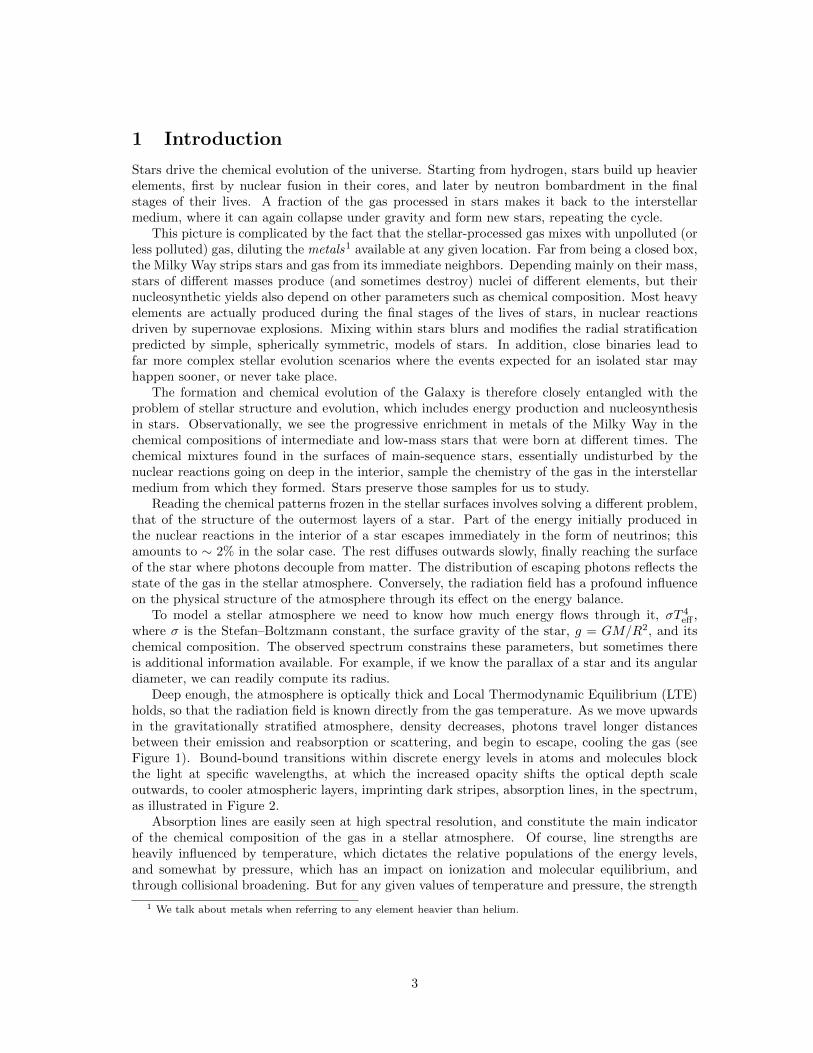
The low viscosity of the stellar plasma, and consequently high Reynolds numbers, is responsiblefor the turbulent behavior of the gas in the solar envelope, including deep photospheric layers.Compared to the classical 1D (hydrostatic equilibrium) models, 3D simulations fully account forthe effect of velocity fields on the atmospheric structure and spectral lines, which get broadenedand (typically) blue-shifted. This is illustrated in Figure 3, where spectra computed for a solar-likestar using a 1D classical model and a CO5BOLD simulation of surface convection are compared.On the other hand, the fact that the model is 3D (spatially) and time-dependent, necessarilyrequires simplifying the calculation of the radiation field to evaluate the energy balance, and theradiative transfer is typically solved for only a few (wisely chosen) frequency bins.

In terms of availability, not all models are made equal. The most complex and costly-to-calculate models tend to be custom-made. On the other hand, large grids of 1D models arepublicly available from Kurucz5 (3500 ≤ Teff ≤ 50 000 K), the Uppsala group 6, and Hubeny &Lanz7 (NLTE models; 15000 ≤ Teff ≤ 55 000 K). Others are available as well, but have beenless frequently used, e.g., the PHOENIX models published by Husser et al. (2013) or those atFrance Allard’s web site.8 Many other families of models, in particular 3D models, are proprietary,but some can be obtained directly from their authors upon request or negotiation. The same istrue for the model-atmosphere codes. Kurucz’s codes and Tlusty are publicly available from thecorresponding web sites9.

5 kurucz.harvard.edu and www.iac.es/proyecto/ATLAS-APOGEE/, but see also www.univie.ac.at/nemo/6 marcs.astro.uu.se7 nova.astro.umd.edu8 http://perso.ens-lyon.fr/france.allard/9 Note that Kurucz’s codes have now been ported to Linux, and there is documentation available. See Section 3.3

8

Figure 3: Spectra in the vicinity of the Ca i λ616.2 nm line computed for a solar-like starusing a classical hydrostatic model (black) and a CO5BOLD hydrodynamical simulation (red;see Tremblay et al., 2013).

2.2 Line formation theory

Radiation plays a key role in determining the atmospheric structure, and therefore has to bedescribed adequately in calculations of model atmospheres. Conversely, once we have a modelstructure it becomes feasible to perform much more detailed radiation transfer calculations topredict stellar spectra. Armed with an appropriate model atmosphere and the necessary line data,we can proceed to compute spectra that can be compared with observations to infer the chemicalmakeup of stars.

The detailed shapes and strengths of spectral lines depend on the thermodynamic structure ofthe atmosphere, which under LTE will dictate the ionization and excitation of atoms and molecules,as well as thermal and collisional broadening. As opposed to the situation with radiative linetransition probabilities, laboratory experiments on line broadening by hydrogen atoms, the mainperturber in solar-like stars, are extremely hard, and the sensitivity of lines to collisions is usuallyderived from calculations, as illustrated, e.g., by Barklem et al. (1998) or Barklem and Aspelund-Johansson (2005). As mentioned in Section 2.1, convective motions in late-type stars will alsodirectly broaden the line profiles, and the lack of them in 1D models is compensated by introducingtwo ad hoc parameters: micro- and macro- turbulence.

Depending on the geometry of the model, the radiative transfer equation for quasi-static con-ditions

∂Iν∂x

= ην − κνIν , (2)

where Iν is the intensity of the radiation field (energy per unit area, per unit of time, per unit

9

of frequency, per unit of solid angle) at a frequency ν, x is the spatial coordinate along the ray,κν is the opacity, and ην the emissivity at that frequency ν, will need to be solved somewherebetween three (three ray inclination angles for a plane-parallel model neglecting scattering) andmillions (3D time-dependent models) of times per frequency. Departures from LTE, considered inSection 2.2.2, usually involve many more calculations, as the statistical equilibrium equations aresolved iteratively, requiring multiple evaluations of the radiation field at all depths.

A number of LTE codes for solving the radiation transfer equation and computing detailedspectra are available. Typically, there is one such code associated with each of the packages usedto compute model atmospheres. For example, there is Turbospectrum for MARCS (Uppsala)models, SYNTHE for Kurucz models, and Synspec for Tlusty models.

2.2.1 Opacity: lines and continua

Under the assumption of LTE, two thermodynamic variables (e.g., temperature and gas pressure)determine the ionization and excitation fractions, which, together with the line collisional broad-ening, can be used to calculate how opaque to radiation is matter. Opacity is characterized bythe likelihood that a photon is absorbed per flying unit length, which is of course a function offrequency: κν . Restricting our discussion to LTE, the thermal component of the emissivity, ην , istrivially calculated from the opacity, as the source function, Sν , is equal to the Planck’s law, andtherefore only depends on temperature

Sν ≡ ην/κν = Bν(T) =2hν3

c21

ehνkT − 1

, (3)

where T is temperature, ν is frequency, c is the speed of light, h is the Planck constant, and k isthe Boltzmann constant.

All absorption is divided into transitions between bound energy levels (lines), or betweenbound levels and the continuum (continua). Transitions between short-lived unbound states, i.e.,the absorption of a photon by an atom, ion, or molecule that temporarily forms by the proximityof two particles (e.g., an atom and an electron in the case of H−), cannot only happen, but maycontribute significant free-free opacity. The strength of a spectral line is critically dependent on theline-to-continuum opacity, and the line opacity can be written as lν = Nα, where N is the numberdensity of absorbers (i.e., the abundance of ions or molecules with the appropriate excitation readyto absorb the photon), and α is the absorption coefficient per absorber (i.e., the cross-section)

α(ν) =πe2

mcfφ(ν) , (4)

where e and m are the charge and mass of the electron, f is the oscillator strength or f -value(proportional to the radiative transition probability A), and φ(ν) is the Voigt function, the resultof the convolution of a Gaussian (due to thermal broadening) and a Lorentzian (due to naturalbroadening and collisional damping), describing the shape of the absorption probability distributionaround the central frequency of the line.

Under LTE, the number density of the absorbers can be split into three factors

N =g

ujNje

− EkT , (5)

where j is the charge (in units of the charge of the electron) of the ion (i.e., j = 0 for neutralatoms), Nj is the abundance (number density) and uj the partition function for the ion j, E isthe energy of the state (above the ground level), and g is its degeneracy. The fraction of nuclei ofa given element that are tied in an ion j is given by Saha’s equation (see Fowler, 2012)

Nj∑iNi

=γjuj∑

i γiuie−

βikT

e−βjkT , (6)

10

where γ = 2/(neh3)(2πmk)

32T

32 , ne is the number density of electrons, and βj =

∑ji=0 χi, where

χi is the energy required to rip an electron from the ion i− 1 (χ0 = 0) in the ground state.Radiative transition probabilities, or f -values, have a direct influence on line strength, just

the same as the number density of absorbers. Unfortunately, only for simple (light) elements it isfeasible to calculate accurately, using quantum mechanics, radiative transition probabilities. Formore complex atoms, most data need to be determined from laboratory experiments, a difficultand time-consuming work. Traditionally, the US National Institute for Standards and Technology(NIST) has done useful compilations, formerly available through a series of books, and now online.10

Kurucz (and colleagues) have made a tremendous effort to augment significantly the number oflines with available transition probabilities, by performing semi-empirical calculations (see, e.g.,Kurucz and Peytremann, 1975), even though those are of significantly lower quality than laboratorymeasurements. Another useful resource for transition probabilities is the Vienna Atomic LineDatabase (Heiter et al., 2008; Ryabchikova et al., 2011, and references therein), which tries tocatch up with the many papers in the literature on line data, whatever its source.

Calculations of bound-free absorption (photoionization) made for light elements (Z ≤ 26) in thecontext of the Opacity Project (OP, see Seaton, 2005; Badnell et al., 2005, and references providedthere), have been available for a long time (Mendoza et al., 2001). This work has been extendedmore recently by the Iron Project team and Sultana Nahar maintains an online database11 (Nahar,2011). The accuracy of the energies computed by these ab initio calculations is about 1%, andtherefore it has been recommended that the photoionization cross-section be smoothed accordingly(see, e.g., Bautista et al., 1998). Allende Prieto et al. (2003) have applied this procedure to the OPdata, and compiled model ions for use with the codes Synspec and Tlusty (Hubeny and Lanz,1995). Free-free absorption, as mentioned above, can be important for abundant species, such asH, H−, or He−. In fact, H− bound-free absorption is the dominant source of continuum opacity inthe optical for the solar photosphere, followed by atomic H, and free-free opacity from the sameion dominates in the IR. Figure 4 illustrates the estimated impact of bound-free absorption bydifferent atoms relative to the total hydrogen (atomic H and H−) continuum opacity on the solarspectrum.

Although we are discussing mainly upward transitions because those are directly observed in thephotospheric spectrum, the opposite downward processes are also taking place – at about the samerate, to have equilibrium. Along with radiative excitation and ionization, we have radiative de-excitation and recombination. Spontaneous (downward) radiative transitions also occur. Finally,collisional processes are always competing, though we do not need to take them into account tocompute the opacity under LTE, as each process is exactly balanced by the opposite, i.e., detailedbalance holds (the sum of all radiative transitions between a given energy state and all others mustbe equal to the sum of radiative transitions from all other states to that one, independently fromthe collisional transitions).

2.2.2 Departures from LTE

Under the assumption of LTE, radiation and matter are coupled locally, and the source function isequal to the Planck function. But no physical law enforces LTE, in particular when the photon’smean free path is long. From a more general perspective, we can consider a case in which the levelpopulations are time independent, i.e., the sum of all radiative and collisional transitions from anenergy level and all others equals the sum of all transitions from all other levels to that one

ni∑j

(Rij + Cij) =∑j

nj(Rji + Cji) , (7)

10 www.nist.gov11 http://www.astronomy.ohio-state.edu/~nahar/nahar_radiativeatomicdata/

11

Figure 4: Impact of continuum opacity of different atoms on the shape of the solar flux relative tothe dominant source of continuum opacity, bound-free H and H− absorption. Image reproducedwith permission from Allende Prieto et al. (2003), copyright by AAS.

where Rij and Cij indicate the radiative and collisional rates, respectively, between the stateslabeled i and j. Note that Rij is closely related to the line absorption coefficient introduced inEq. (4); it is proportional to the product of α times the photon density, integrated over the lineprofile (plus a contribution from spontaneous emission if i > j). The system of equations 7 for nstates includes n − 1 linearly dependent equations, and therefore it needs to be closed by addinga total particle number conservation equation.

Solving the statistical equilibrium equations requires many data which are not needed underLTE. To evaluate all possible transition rates across states and ions we need not only radiativecross-sections (i.e., transition probabilities and photoionization cross sections) but also collisionalstrengths (collisional transition probabilities, if you will). Given their high density, electrons andhydrogen atoms are the main particles responsible for inelastic collisions. As discussed in Sec-tion 2.2 for line broadening (elastic collisions), laboratory experiments on inelastic collisions withatomic hydrogen are very hard to carry. Approximate formulae exist for electron-impact collisionalexcitation and ionization (see Allende Prieto et al., 2003), although these are, at best, only good toprovide order-of-magnitude estimates. Quantum mechanical calculations of atomic structure canprovide much better estimates for collisional strengths for electron impacts (see, e.g., Zatsarinnyand Tayal, 2003; Barklem, 2007a; Belyaev et al., 2014; Osorio et al., 2015), but more involvedmethods, requiring an adequate knowledge of the relevant molecular potentials, are needed toderive reliable estimates for hydrogen collisions (e.g., Krems et al., 2006; Barklem et al., 2012).

Under solar photospheric conditions, hydrogen atoms dominate by number over free electrons,but inelastic hydrogen collisions tend to have a limited role on line formation (Allende Prieto et al.,2004a; Pereira et al., 2013). Figure 5 illustrates, however, that their effect is visible in the changes

12

of strength experienced by lines such as the O i triplet at 777 nm as a function of heliocentricangle. At lower metallicities, higher pressure and a lower density of free electrons combine to makethe role of hydrogen collisions much more important, as discussed for example by Gratton et al.(1999). Shchukina et al. (2005) predict abundance corrections due to NLTE effects on Fe i in themetal-poor subgiant HD 140283 as large as 0.6 dex for a 1D model atmosphere, and as large as0.9 dex for a 3D model, in the absence of inelastic hydrogen collisions.

Figure 5: Observed behavior of the the O i triplet at 777 nm in the Sun as a function of theinclination of rays from the solar surface (µ = cos θ, where θ is the angle between the observer andthe normal to the solar surface). The filled circles correspond to observations, and the solid lines tomodels. The observations at disk center (µ = 1) are reproduced in all cases, by changing the oxygenabundance, and the comparison near the limb (µ = 0.32) tests the realism of the calculations. Thebehavior of the lines can be reproduced considering inelastic collisions with hydrogen atoms inthe rate equations. The factor SH is introduced to enhance the approximate collisional rates froma Drawin-like formula as proposed by Steenbock and Holweger (1984). Image reproduced withpermission from Allende Prieto et al. (2004a), copyright by ESO.

Departures from LTE can be very important in some situations. If they involve importantspecies (say, hydrogen, helium, iron), their impact can be profound and the statistical equilibriumequations may need to be solved together with the model atmosphere problem, as it is usually donefor hot stars. In many other cases, the departures affect trace species and particular transitionsof interest, which may induce a modest effect on the overall atmospheric structure, but anywaymust be considered in order to avoid large systematic errors in the calculated line profiles, andtherefore the derived abundances. In this latter case, one can adopt the thermal structure of theatmosphere plus a second thermodynamic variable (usually the electron density) and solve thestatistical equilibrium equations (7) for the relevant ions in isolation from the model atmosphere,what is usually referred to as the restricted NLTE problem.

There are NLTE codes available for solving the full NLTE problem (statistical equilibrium plusatmospheric structure) and some limited to the restricted NLTE problem. Among the former, wefind the publicly available codes CMFGEN12 (Hillier, 2012) the suite of Munich codes13 (Pauldrachet al., 1998), and Tlusty14 (Hubeny and Lanz, 1995), three packages originally developed in thecontext of hot stars. The code MULTI15 (Carlsson, 1992) deals with the restricted NLTE problem,and has been widely used in the context of late-type atmospheres.

12 http://kookaburra.phyast.pitt.edu/hillier/web/CMFGEN.htm13 http://www.usm.uni-muenchen.de/people/adi/Programs/Programs.html14 http://nova.astro.umd.edu/15 http://folk.uio.no/matsc/mul22/

13

3 Working Procedures

With the basic blocks described above – adequate opacities, and codes to compute model atmo-spheres and spectra – the only remaining input is an observed spectrum, and a work plan.

The various elements entering in the analysis are tightly coupled. To calculate a model at-mosphere, we need to know the basic atmospheric parameters and abundances, precisely the veryvariables we seek to derive from the spectral analysis. Thus, it is only natural to address theproblem iteratively. First, atmospheric parameters are guessed, then a spectrum computed andconfronted with the observations to determine the parameters, repeating the cycle as needed. Suchprocess can, in some situations, be simplified, provided we are confident that some parameters aredecoupled from others – for example, when we derive the abundance of iron in a solar-like star fromlines of singly-ionized Fe ions, which have only a weak sensitivity to the surface gravity. In somecases, parameters derived from external data, free from systematic errors that model spectra aresubject to, are preferred, and that also simplifies the analysis, eliminating the need for iteration.

The amount of information available directly from a spectrum will be limited by its spectralcoverage, signal-to-noise, and resolution.16 In addition, spectra show a strong response to someparameters (e.g., the effective temperature), and a much weaker or null reaction to others (e.g.,the abundance of ytterbium). Tracking correlations is extremely important to arrive at reliableuncertainty estimates in the inferred abundances.

Because of the low temperature and shallow temperature structure in the outer layers of thephotosphere, lines with fairly opaque cores saturate, i.e., their strength does not grow linearlywith the abundance of the absorbers, and therefore relatively weak lines are preferred. Weaklines demand high spectral dispersion, which usually implies narrow spectrograph slits and highfrequency variations in the instrument’s throughput (i.e., poor accuracy in flux calibration), andmore limited spectral windows. For this reason, the analysis of high-resolution spectra is usuallysupplemented with lower-dispersion spectrophotometry or photometry.

In what follows, we will briefly split the abundance determination process into three steps:gathering data, choosing atmospheric parameters, and deriving abundances.

3.1 Obtaining stellar spectra and reference data

Because the atmospheric parameters are related to the fundamental stellar parameters, and thesecan be constrained from many other data independent from spectra, we should compile all therelevant information available from the literature. If we aspire to provide a physically consistentpicture of the observed objects, the atmospheric parameters used in the spectroscopic analysis needto be consistent both with the spectrum and with the available external data, whenever possible.

Examples of useful data are: trigonometric parallaxes from astrometric measurements, angulardiameters from interferometry, or mean densities from asteroseismology (see, e.g., Bruntt et al.,2010a; Pinsonneault et al., 2014; Coelho et al., 2015; Silva Aguirre et al., 2015). However, be awarethat in most cases deriving fundamental quantities such as radii, masses, or distances from theseobservations involves to some extent the use of models of stellar structure and evolution, subjectto their own issues and systematic errors. If the stars of interest are members of binary systems,there may be very useful constraints on the stellar masses from the system dynamics, and if we arelucky enough to have an eclipsing system, then masses and radii may be constrained with exquisiteaccuracy (Popper, 1980; Andersen, 1991; Torres et al., 2010), but the likelihood for such alignmentis very low.

Digital data can be handled and stored with ease, and as instruments become more efficientand observations more homogeneous, there are more and more data archives that offer collections

16 One may define a power-to-resolve P that combines these three parameters to quantify approximately theinformation content in a spectrum (Allende Prieto, 2016).

14

of stellar photometry and spectra of different kinds. In Section 4.1 we provide a list of some of themost popular collections of spectra for nearby and bright stars.

Photometric information, and most of all, spectrophotometric information, is of high value whenit comes to constraining atmospheric parameters, in particular effective temperature, although theinterstellar extinction complicates the analysis. There are large libraries with spectrophotometryfor stars, some of which are mentioned in Section 4.1.

A word should be said here about photometric calibrations for deriving stellar effective tem-peratures from photometry. Direct calibrations are rarely used, due to the high sensitivity of themodel atmospheres and irradiance calculations to the input physics, and in particular the equa-tion of state. The most widely-used calibrations are based on the so-called infrared flux method(Blackwell et al., 1980; Alonso et al., 1999; Ramırez and Melendez, 2005; Gonzalez Hernandez andBonifacio, 2009; Casagrande et al., 2010), which exploits a more robust prediction from the models,the ratio of the monochromatic flux at a given infrared wavelength to the bolometric flux of a star.

In many cases, spectra for the stars of interest are not available from existing data bases, and wewill need to obtain new observations. Observing facilities are continuously progressing. However,spectral resolution is not increasing as spectrographs become larger to mate with larger telescopes.For a given grating, the product of the resolving power and the slit width are proportional tothe ratio of the collimator and telescope diameters, making it difficult to reach high dispersionwithout using narrow slits and losing light. In addition, there has only been modest progress infeeding multiple objects to high-resolution spectrographs, at least in comparison with the massivemultiplexing capabilities now available and planned for lower dispersion instruments.17 Manyobservatories offer high-resolution spectrographs, but reviewing the existing choices is out of thescope of this paper. We will go back to discussing some of the largest projects, ongoing andplanned, in Section 4.

3.2 Atmospheric parameters

Provided with a wide spectral range, it may be feasible and convenient to derive all the relevantatmospheric parameters needed to calculate a model atmosphere from the very same high-resolutionspectra that will be later used to derive abundances. Nevertheless, alternative paths are usefulfor two reasons: as a sanity check (remember that the analysis of the high-resolution spectra willhave associated caveats, as it involves many approximations), or simply because a high-resolutionspectrum will have a limited sensitivity to some parameters, with surface gravity being the mosttypical case. We mentioned in the previous section several possibilities to constrain the atmosphericparameters from measurements other than high-resolution spectra. Here we will highlight the mostuseful features available in spectra when lines are resolved.

The effective temperature is usually derived from the excitation balance of atomic iron, calcium,silicon or titanium, i.e., by requiring that lines with different excitation energy give the sameabundance. This technique simply takes advantage of the Boltzmann equation [see Eq. (5)], whereT is the temperature in the relevant atmospheric layers for the lines, which is of course tightlycoupled to the effective temperature of the star Teff . Unfortunately, the de-saturation of stronglines induced by small-scale motions of the iron atoms (micro-turbulence), complicates somewhatthe performance of this method, which is sensitive to this parameter, as well as to departures fromLTE.

The damping wings of hydrogen lines, largely controlled by Stark broadening induced by elasticcollisions with free electrons, but also affected by collisions with the surrounding hydrogen atoms,are also highly dependent on the thermal structure in layers close to Rosseland optical depth τ ∼ 1,which provides an excellent thermometer (see Fuhrmann et al., 1993, 1994; Barklem et al., 2000,

17 MUSE for the VLT employs image slicers to feed 24 spectrographs at once (Bacon et al., 2012), and VIRUSfor the Hobby-Eberly telescope has some 30 000 fibers feeding 75 spectrographs simultaneously (Hill et al., 2012).

15

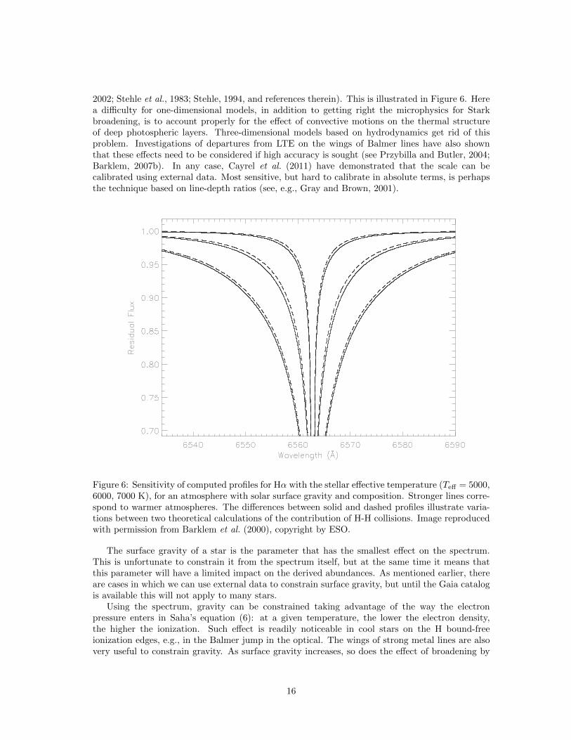
2002; Stehle et al., 1983; Stehle, 1994, and references therein). This is illustrated in Figure 6. Herea difficulty for one-dimensional models, in addition to getting right the microphysics for Starkbroadening, is to account properly for the effect of convective motions on the thermal structureof deep photospheric layers. Three-dimensional models based on hydrodynamics get rid of thisproblem. Investigations of departures from LTE on the wings of Balmer lines have also shownthat these effects need to be considered if high accuracy is sought (see Przybilla and Butler, 2004;Barklem, 2007b). In any case, Cayrel et al. (2011) have demonstrated that the scale can becalibrated using external data. Most sensitive, but hard to calibrate in absolute terms, is perhapsthe technique based on line-depth ratios (see, e.g., Gray and Brown, 2001).

Figure 6: Sensitivity of computed profiles for Hα with the stellar effective temperature (Teff = 5000,6000, 7000 K), for an atmosphere with solar surface gravity and composition. Stronger lines corre-spond to warmer atmospheres. The differences between solid and dashed profiles illustrate varia-tions between two theoretical calculations of the contribution of H-H collisions. Image reproducedwith permission from Barklem et al. (2000), copyright by ESO.

The surface gravity of a star is the parameter that has the smallest effect on the spectrum.This is unfortunate to constrain it from the spectrum itself, but at the same time it means thatthis parameter will have a limited impact on the derived abundances. As mentioned earlier, thereare cases in which we can use external data to constrain surface gravity, but until the Gaia catalogis available this will not apply to many stars.

Using the spectrum, gravity can be constrained taking advantage of the way the electronpressure enters in Saha’s equation (6): at a given temperature, the lower the electron density,the higher the ionization. Such effect is readily noticeable in cool stars on the H bound-freeionization edges, e.g., in the Balmer jump in the optical. The wings of strong metal lines are alsovery useful to constrain gravity. As surface gravity increases, so does the effect of broadening by

16

collisions between the absorber and H (and partly He) atoms, enhancing the wings of metal lines,as illustrated in Figure 7 for one of the lines of the Mg ib triplet in the spectrum of the metal-poorstar BD+17 4708.

Figure 7: The top panel shows part of the spectrum of the metal-poor star BD+17 4708, while thebottom panel provides a close view of one of the Mg ib lines in the spectrum of the star comparedwith calculations for models with a range in surface gravity. The analysis focuses on the wings,since the line core is not matched due to departures from LTE. Image reproduced with permissionfrom Ramırez et al. (2006), copyright by ESO.

The overall metallicity, usually approximated by the iron abundance, is derived, like any otherabundance, from lines of weak-to-moderate strength. This is either done from equivalent widthsor line profiles, but this choice will be further discussed in the next section.

3.3 Determining abundances from spectra

Once we have decided on the best set of atmospheric parameters for a star which, we recall, arelikely to be revised during the analysis, we can proceed calculating, or obtaining from a database, an appropriate model atmosphere. Of course, if some or all of the atmospheric parametersare constrained from observed line strengths, as opposed to other external information such asphotometry, spectrophotometry, or astrometry, we will need the model atmospheres earlier in theprocess. Any theoretical fluxes to be compared to observations, i.e., photometry or spectrophotom-etry, also require model atmospheres, but unlike high-resolution spectra, these fluxes are usuallyavailable together with the libraries of model atmospheres, and one does not need to calculatethem in most instances.

17

Depending on the type of star, the accuracy being sought, more mundane factors such asaccess to computing resources and human collaborators, we should decide on the type of modelatmosphere to adopt, and how to secure it. We have already mentioned the most widely usedpossibilities in Section 2.1.

The Kurucz codes have been used in modern operating systems, and are publicly available(e.g., from Castelli’s site18). The MARCS code is not, although custom-made models are kindlyprovided by the core MARCS community – mostly residents or former residents of the Swedishtown of Uppsala. There are many different interpolation tools that have been used in the literature,although few are publicly available and documented. An interpolation code for MARCS models isavailable from the MARCS site, and others for Kurucz’s models are available from A. McWilliamand from me.19

As mentioned earlier, in addition to a model atmosphere, deriving abundances requires basicdata associated with the atomic or molecular transitions we plan on using as diagnostics: wave-lengths, transition probabilities, the energy of the lower level connected by the transition, anddamping constants. With these inputs, we have all we need to calculate a model spectrum, sinceother auxiliary data are typically included in radiative transfer codes. Once we are able to computemodel spectra, we can iteratively compare those with observations to infer the chemical composi-tions of stars. Section 3.4 is devoted to tools commonly used for these tasks.

3.4 Tools for abundance determination

As outlined above, the process of abundance determination requires a certain degree of iteration.At the very least, when the atmospheric parameters are well constrained, and the overall metalcontent of the star is known in advance, we need to iterate the last step of calculating a syntheticspectra to arrive at the chemical composition that best matches the observations.

Traditionally, for the analysis of a small number of spectra, iterations are performed underthe careful control of a person. The basic workhorse software is a radiative transfer code, thatpredicts what the observed spectrum would look like for a given model atmosphere and chemicalcomposition. We mention the most popular choices (there are many more!) in Section 3.4.1. Whenthe number of spectra to analyze is very large, a manual analysis using interactive software is nolonger possible, and more powerful tools become necessary. These are the subject of Section 3.4.2.

3.4.1 Interactive tools

The fundamental tool for chemical analysis is a spectral synthesis code. For a fixed set of inputdata: model atmosphere, and atomic and molecular line and continuum opacities, the code can beused to predict spectra for different abundances to identify the value that matches observations– one or an array of absorption lines. Some of the most commonly used spectral synthesis codespublicly available have already been mentioned in Section 2.2: these are MOOG20 (Sneden, 1974),Synspec21 by Hubeny & Lanz, Turbospectrum22 by Plez (2012) (see also Alvarez and Plez,1998). Many more codes are available but less frequently used, for example MISS by Allende Prietoet al. (1998) (see also Ruiz Cobo and del Toro Iniesta, 1992), RH by Uitenbroek23, ASSET byKoesterke (2009), or SPECTRUM24 by R. O. Gray.

18 http://wwwuser.oat.ts.astro.it/atmos/ and http://wwwuser.oat.ts.astro.it/castelli/19 See kmod.pro at http://www.as.utexas.edu/~hebe/stools/20 http://www.as.utexas.edu/~chris/moog.html21 http://nova.astro.umd.edu/Synspec49/synspec.html22 http://www.pages-perso-bertrand-plez.univ-montp2.fr/23 http://www4.nso.edu/staff/uitenbr/rh.html24 http://www.appstate.edu/~grayro/spectrum/spectrum.html

18

Using line equivalent widths (the total absorption associated with a spectral line) is opera-tionally convenient (one number per transition instead of an array of fluxes) and makes the resultsindependent from macro-turbulence and rotational broadening. For those reasons, despite it repre-sents a loss of information, equivalent widths are still used in many studies. This requires measuringline equivalent widths in both observed and model spectra. One of the software packages commonlyused to measure manually equivalent widths is the splot package within IRAF.25 Codes such asMOOG can be used to provide abundances directly from equivalent widths (see Section refauto-mated). This modus operandi is highly effective for processing large numbers of transitions formany stars, and it has been used with success in numerous projects (see, e.g., Reddy et al., 2003;Bensby et al., 2003; Santos et al., 2004; Fulbright et al., 2010; Nissen, 2015, to mention a fewexamples).

3.4.2 Automated tools

There are several codes that automate the measurement of equivalent widths. The most used onesare ARES (Sousa et al., 2007) and DAOSPEC (Stetson and Pancino, 2008; Cantat-Gaudin et al.,2014). As already mentioned, the derivation of abundances from observed equivalent widths hasbeen automated for a long time in codes such as MOOG or those in the Uppsala package. Theautomation of the task of directly fitting spectra with models has a more recent history.

Spectroscopy Made Easy26 by Valenti and Piskunov (1996) is a package for fitting spectraby wrapping an optimization algorithm around a spectral synthesis code. ULySS27 by Kolevaet al. (2009) is also spreading in use. FERRE28 by Allende Prieto et al. (2006) includes severalalgorithms and is optimized for dealing with large samples. Another option is VWA29 by Brunttet al. (2010b). Many more packages of general application have been employed in the literature, butthey are not publicly available, e.g., MATISSE by Recio-Blanco et al. (2006), TGMET30 by Katzet al. (1998), or MyGIsFOS by Sbordone et al. (2013). Some packages have been developed forparticular instruments or projects, such as various parts of the SEGUE Stellar Parameter Pipeline(Lee et al., 2008a,b; Allende Prieto et al., 2008; Lee et al., 2011a), or the original RAVE analysispipeline (e.g., Boeche et al., 2011; Siebert et al., 2011).

Although these tools are very useful to deal with large samples, one should avoid using themblindly. There is no substitute for understanding which spectral features can be modeled accuratelyand which ones cannot. The importance of checking thoroughly, using well-studied stars, theperformance of an automated tool on a particular data set, cannot be overemphasized.

25 IRAF (Image Reduction and Analysis Facility) is distributed by the National Optical Astronomy Observatory,which is operated by the Association of Universities for Research in Astronomy (AURA) under cooperative agreementwith the US National Science Foundation.

26 http://www.stsci.edu/~valenti/sme.html27 http://ulyss.univ-lyon1.fr/28 http://hebe.as.utexas.edu/ferre29 https://sites.google.com/site/vikingpowersoftware/30 http://www.obs-hp.fr/guide/elodie/tgmet-doc/TGMET1.HTML

19

4 Observations

There is a wide variety of collections of spectra readily available on the internet. This includeslibraries with typically high-quality data for specific sets of stars, and data repositories for largesurveys. We describe the most significant ones below, as well as the most exciting instruments nowin operation or being planned for the future.

4.1 Libraries

If you are interested in a bright star, its high-resolution optical spectrum may be available inthe Elodie archive31 (Moultaka et al., 2004), S4N32 (Allende Prieto et al., 2004b), the UVES-Paranal library33 (Jehin et al., 2005), or the Nearby Stars Project34 (Luck and Heiter, 2005). Ifthe spectrum has been ever obtained with HST, you will find it in MAST,35 and if it has beensecured in recent times with ESO instruments, there is a good chance it is publicly available in theESO archive36, although you may need to reduce the data yourself. Other observatories have theirown archives, and very many are now becoming publicly available, but they are too many to listhere, and their reservoir of public high-dispersion spectra is anyway limited. A new library underdevelopment at Leiden is based on observations with X-Shooter, offering a wide spectral coverageat medium-high resolving power (Chen et al., 2012).

Regarding spectrophotometry, it is worthwhile to highlight the Indo-US library37 by Valdeset al. (2004), and MILES38 by (Falcon-Barroso et al., 2011, and references therein) from the ground,and the STIS Next Generation Spectral Library39 by Gregg et al. (2006) and Heap and Lindler(2007) from space. The ESA mission Gaia should bring accurate parallaxes and spectrophotometry(with very low resolution though) for 109 stars before the end of the decade (Lindegren et al., 2008),but we will come back to this important observatory in Section 4.3.

4.2 Ongoing projects

We live in a time when instruments with high multiplexing capabilities are revolutionizing thestudy of the chemical compositions of stars in the Milky Way and other nearby galaxies. For themost part, the distinction between instruments and surveys is blurred, since these instrumentsserve mainly a single or a small number of projects.

For the sake of limiting the size of this article, we will concentrate on the largest projects andthe instruments with the largest multiplexing capabilities currently in operation, and which arebeing massively used for the acquisition of stellar spectra that have become or will soon becomepublic, at the expense of leaving out excellent instruments that do not meet those conditions.

The Sloan Digital Sky Survey (SDSS; York et al., 2000) is the most dramatic example of amodern survey making efficient use of a suite of instruments. In addition to five-band photo-electric photometry of a third of the sky, the SDSS has obtained R = 2000 spectra for severalmillion galaxies and about a million stars since it started operations in 2000. The project uses adedicated 2.5-m telescope (Gunn et al., 2006) with a field-of-view of 7 square degrees. Originallyequipped with two double-arm spectrographs (Smee et al., 2013), fed by 640 fibers, and subse-quently upgraded to 1000, providing a wide spectral coverage (360 – 1000 nm approximately) the

31 http://atlas.obs-hp.fr/elodie/32 http://hebe.as.utexas.edu/s4n/33 https://www.eso.org/sci/observing/tools/uvespop/interface.html34 http://bifrost.cwru.edu/NStars/35 https://archive.stsci.edu/36 http://archive.eso.org/cms.html37 http://www.noao.edu/cflib/38 http://www.iac.es/proyecto/miles/pages/stellar-libraries/miles-library.php39 https://archive.stsci.edu/prepds/stisngsl/

20

project concentrates on stars in the magnitude range 14 < V < 21. These data have been used forstudying the structure of the Milky Way disk and halo in a series of papers (see, e.g., Allende Prietoet al., 2006; Schlaufman et al., 2009; Bond et al., 2010; Schlaufman et al., 2011; Lee et al., 2011b;Cheng et al., 2012; Schlaufman et al., 2012; Schlesinger et al., 2012; Fernandez-Alvar et al., 2015;Lopez-Corredoira and Molgo, 2014), but many more studies are to be expected as observationscontinue (at least to 2020). SDSS releases their data publicly every one or two years, a move thathas been decisive in making it one of the most scientifically productive observatories in the world.

A few years ago, SDSS added a new instrument optimized for the observation of stars in theH-band (1.5 – 1.7 µm) at high R = 22 500. The Apache Point Galactic Evolution Experiment(APOGEE) has collected so far nearly half a million spectra for some 100 000 stars in the MilkyWay (see Holtzman et al., 2015; Majewski et al., 2015) and results are already appearing on varioussubjects (see, e.g., Deshpande et al., 2013; Majewski et al., 2013; Frinchaboy et al., 2013; Meszaroset al., 2013; Zasowski et al., 2013; Garcıa Perez et al., 2013; Bovy et al., 2012; Nidever et al.,2014; Hayden et al., 2015). The project will expand this collection of spectra by a factor of severalbetween 2014-2020, including observations from Las Campanas, accessing the Magellanic clouds,parts of the disk not available from the North, and getting a better perspective of the central partsof the Milky Way. In the SDSS tradition, APOGEE’s spectra and derived data products are madepublic on a regular basis.

The Radial Velocity Experiment (RAVE) (see, e.g., Kordopatis et al., 2013a, and referencestherein), already done with the data taking, has targeted stars with brighter magnitudes (5 <V < 14) and therefore located at closer distances, with higher resolution R = 8500 and a narrowerspectral range (837 – 874 nm) than SDSS. The results from the survey are already coming out,(among their most recent publications see, e.g. Kordopatis et al., 2013a; Piffl et al., 2014; Conradet al., 2014; Kordopatis et al., 2013b; Kos et al., 2013; Williams et al., 2013) and the associatedspectra for about half a million stars will probably become public sometime in the future.

The Large Area Multi Object fiber Spectroscopic Telescope (LAMOST) resembles in manyrespects SDSS but with 4000 fibers, an original telescope with an effective aperture between 3.6 –5.9 m, and a robotic fiber positioner. After some difficulties the project is now starting to showresults (see, e.g., Yi et al., 2014; Yang et al., 2014; Ren et al., 2013; Zhang et al., 2013; Zhao et al.,2013; Liu et al., 2015), and a lot more is envisioned to come out in coming years.

The Gaia-ESO Survey (GES) is a massive ESO public survey that is using 300 nights on theVery-Large Telescope to obtain high-resolution spectra for about 100,000 stars (Gilmore et al.,2012), thought out to complement the observations from Gaia (see Section 4.3). About 90% ofthe observations are made at a resolving power of about 15,000 with the GIRAFFE spectrograph(Hammer et al., 1999; Blecha et al., 2000), and the remainder at higher resolution with the cross-dispersed UVES spectrograph (Dekker et al., 1992; Hammer et al., 1999). It involves a largeEuropean collaboration, and has two distinct parts, one focusing on field stars and a second onedevoted to clusters. The observations started at the end of 2012, the raw spectra are quickly madepublic on the ESO archive, and the advanced data products (fully reduced spectra, radial velocitiesand stellar parameters including abundances) are following on a fast-paced schedule. There arealready plenty of examples of science results from this project (e.g., Magrini et al., 2015; Lindet al., 2015; Sacco et al., 2015).

The GALactic Archaeology with HERMES project (GALAH) (see Zucker et al., 2013) expandson the idea of chemical tagging and producing a chemical map of stars in the Galaxy to provideoptical high-resolution spectroscopy (R = 28 000) for over a million stars using the 4-m AATtelescope in Australia. The HERMES instrument was commissioned at the end of 2013, and thefirst results are eagerly expected.

The Hobby-Eberly Telescope Dark Energy Experiment (HETDEX; Hill et al., 2012), althoughconceived mainly as a cosmology project, leaves no star behind, at least of those that fall on theirIntegral-Field Units during the course of the experiment, which last five years. These spectra will

21

be deep (V < 22) and reach into the UV (350 – 550 nm), although of low resolution (R = 700), withthe particular plus of having no selection biases (like Gaia). As of this writing the observationsare a few months from starting.

4.3 In the future

If current and ongoing surveys are tremendously exciting, there are instruments in the design andconstruction phase that will make the future even more thrilling. Having in mind that this is alive review, and accepting the task of coming back to complete information as time progresses, thefollowing paragraphs will only mention projects that are subjectively perceived by this writer asthe most promising ones.

Gaia has long been declared as the ultimate survey of the Milky Way. There is no doubtthat Gaia’s capabilities are impressive. The satellite was launched in December 2013, and thefirst catalog is expected in 2016. This ESA cornerstone mission is building a full-sky catalog ofthe stars in the Milky Way with a unique suite of instruments that provide exquisite astrometry,and (spectro-)photometry for about 109 stars, and high-resolution spectroscopy (847 – 874 nm)for about 108 stars. Rather than providing all the details on Gaia, I will simply refer the readerto Lindegren et al. (2008), but not without noting that all other spectroscopic efforts are largelycomplementary to Gaia, since its high-resolution spectrograph is only effective to provide radialvelocities for a small fraction of the sample, due to the short integration times and the implied lowsignal-to-noise ratio of the spectra.

The Dark Energy Spectral Instrument (DESI; Levi et al., 2013) is an ambitious project con-ceived as a natural follow-up of the Baryon Oscillations Spectroscopic Survey (BOSS; Schlegelet al., 2007; Eisenstein et al., 2011), part of the SDSS. Improving on telescope area (from the2.5-m SDSS telescope to the 4-m Mayall telescope at Kitt Peak), doubling spectral resolution,enhancing multiplexing capabilities (from 1000 to 5000 fibers, from plug-plates to a robotic po-sitioner), all without losing field of view and synoptic operations. Like BOSS and the follow-upeBOSS project, DESI will mainly measure redshifts to identify the imprint left by primordial bary-onic acoustic oscillations on large scale structure, but there is no doubt that this instrument willalso make an important contribution for Galactic studies of stars.

In addition to DESI, there are other instruments planned for 4-m-class telescopes. Theseinstruments have somewhat more modest multiplexing capabilities but differ from DESI in thatthey provide various spectral settings, allowing higher resolution observations, and therefore willenable stellar science that DESI cannot do, and smaller, more targeted projects. These are WEAVEfor the 4.2-m WHT in La Palma (Dalton et al., 2014), or 4MOST for the 4-m VISTA at Paranal(de Jong et al., 2014). Yet another high-multiplexing spectrograph with the ability of reaching aresolving power of R = 20 000 in the infrared for up to ∼ 1000 targets simultaneously, MOONS, isprojected for the 8-m ESO VLT (Cirasuolo et al., 2014; Oliva et al., 2014).

One can imagine the ultimate spectroscopic experiment, let’s call it the Final Uniform Spec-troscopic Survey, using a Field Ultra-dense Survey Spectrograph (FUSS), a natural endpoint of allthe surveys described above, providing radial velocities and chemistry to complement Gaia’s as-trometry and photometry. This would consist of a pair of large-field large-aperture telescopes (oneper hemisphere), perhaps 6 to 8-m-class, resembling the LSST, with massive integral field units(IFU) covering their entire field of view a la VIRUS (the HETDEX spectrograph), surrounded bya farm with tens of thousands of compact fiber-fed spectrographs. Over the course of the project,probably about a decade, these telescopes would scan the entire sky once, getting spectra of ev-erything down to V = 20 mag. This project has not yet been seriously proposed, but I would besurprised if it is not started by 2025!

22

4.4 Examples of recent applications

The analysis of stellar spectra to derive chemical compositions of stars has led, in the last decade,to vast progress across fields in astrophysics. With the aim of highlighting practical applicationsof stellar photospheric abundances, a series of topics that are the subject of active research arebriefly presented below. These are only a few examples, and other writers would surely chooseother topics.

4.4.1 The Galactic disk

Stars in the Galactic disk were found to split nicely into two components with densities fallingexponentially from the plane and scale heights of about 0.3 (thin disk) and 1 kpc (thick diskGilmore and Reid, 1983). The spectroscopic studies of these populations carried out in the lastdecade have also shown a split in their α-element (O, Mg, Si, Ca, Ti) to iron abundance ratios, aswell as in age, with stars in the thick disk being fairly old (> 8 Gyr) and those in the thin diskyounger, between 1 – 8 Gyr (see, e.g., Fuhrmann, 1998; Bensby et al., 2003; Reddy et al., 2006;Allende Prieto et al., 2006; Adibekyan et al., 2013; Nidever et al., 2014; Anders et al., 2014; Ruchtiet al., 2015).

Despite the rich information available from spectroscopic data, it is yet unclear how this two-component structure came together, and even whether the two disks are intimately connected ornot. It is recognized that gas accretion from early galactic neighbors and radial migration of starsin the disk must have played a role, but the sequence of events that gave rise to the present-dayGalactic disk has so far evaded our understanding. This is an area where the data flow from Gaiaand the spectroscopic surveys mentioned above, hand by hand with models and simulations, willlikely be of great help in the following years.

4.4.2 Globular clusters

For the most part of the 20th century, globular clusters were considered groups of stars sharingage and chemical composition. Unlike Galactic (open) clusters, globulars are old and metal-poor,associated with the Milky Way halo (or thick disk), and as such are excellent probes to study theearly evolution of the Galaxy. Then we came to realize that was not true. Star to star variationsin some elements became apparent. Sodium to oxygen or magnesium to aluminum correlations.Even worse, space-based photometric studies revealed multiple sequences, suggestive of differenthelium fractions, in the most massive clusters (see, e.g., Norris, 2004).

The details of how globular clusters formed remain elusive, but it seems clear that some of thestars in the clusters formed from gas that has been polluted by previous cluster stars (Grattonet al., 2004). Furthermore, at least some of the most massive globular clusters in the Milky Wayappear to be the remnants of small galaxies that ended up torn apart in the Galactic potential(Bellazzini et al., 2003).

4.4.3 The most metal-poor stars

Since the chemical composition of the Universe after the primordial nucleosynthesis following theBig Bang was basically hydrogen and helium, the overall lack of heavier elements in a star can beinterpreted as a sign of a primitive composition and a very old age. Observational cosmology hastraditionally targeted galaxies at high redshift, but the objects with the most primitive composi-tions have been found right here in the Milky Way. These are extremely metal-poor stars withiron-to-hydrogen ratios orders of magnitude lower than the Sun: up to 7 orders of magnitude inthe case of the star recently discovered by Keller et al. (2014).

23

The relative numbers of stars with different metallicities in the halo constrain the star formationhistory and initial mass function in the early Milky Way. Furthermore, the oldest stars in theGalaxy can inform us about what happened in the early Universe.

For stars to form, the gas in the interstellar medium needs to cool down for gravity to win overpressure. At very low metallicity, the lack of lines from metals makes it very difficult for gas toradiate and cool down. As a result, massive stars form, but no low-mass stars, producing a massdistribution shifted to higher masses than what we observe today in the disk of the Milky Way(Bromm and Larson, 2004). The discovery a few years ago by Caffau et al. (2012) of a dwarf starin the halo with an overall metallicity of [Fe/H]' −4 sets an upper limit to where that thresholdcan be, constraining theories of star formation.

4.4.4 Solar analogs

Uncertainties in atomic and molecular data, especially oscillator strengths, directly propagate intothe derived abundances from stellar spectra. That applies to absolute abundances. However, in adifferential analysis between two stars that are very similar, systematic errors cancel out.

Differential studies between the Sun and similar stars can render a precision in the derivationof atmospheric parameters at the level of a few K in Teff and 0.01 dex in log g, which are alsoaccurate to that level, since the absolute surface temperature and gravity of the Sun are knowneven better. In this fashion, relative abundances can be derived to better than 0.01 dex in [Fe/H]Nissen (2015), or more than 10 times better than absolute abundances.

This level of precision opens new opportunities for discovery in astrophysics. Detailed studiesof nearby stars with parameters very close to solar have shown that there are subtle differencesin composition between most of them and the Sun (Melendez et al., 2009; Ramırez et al., 2009),which may be related to the sequestration in rocks or rocky planets of refractory elements that donot make it into the star. Needless to say, we look forward to future applications of this techniqueto other types of stars.

5 Reflections and Summary

The analysis of the chemical compositions of stars evolved from early experiments by Bunsen,Kirchhoff and Fraunhofer in the 19th century into a quantitative field through the theoreticalfoundations provided by Schwarzschild, Eddington, Milne, and others. The LTE numerical codesfor computing model atmospheres developed in the 1970s and 80s, mainly by Gustafsson andKurucz, set the standard for modern analyses of AFGKM-type stars, while NLTE codes weredeveloped for warmer ones. Atomic and molecular data, at a modest pace, has been perhapsthe most significant improvement in modeling late-type stellar spectra over the last two decades,with the exception of the development of hydrodynamical models, which represent a dramaticadvancement in our ability to match in close detail spectral line shapes, even though their overallimpact on the inferred abundances is limited.

The rate at which spectroscopic observations are gathered has been revolutionized, and a fewindividual projects have obtained more spectra in the last few years than the accumulated datafrom previous history. These projects are providing vast and homogeneous data sets, which havenot been fully explored, while new and larger projects are appearing in the scene. In response,spectral analysis software is being transformed from interactive tools to industrial chain processing.

The extraordinary new observations soon to become available from the Gaia mission, andthe constraints on atmospheric parameters for individual stars that they will provide, will helpenormously to uncover the deficiencies of standard analyses, driving improvements in modelingspectra. The new spectroscopic data from large ongoing and upcoming ground-based surveys will

24

slowly but surely enlighten our understanding of the formation and evolution of the Milky Way,and as result, of galaxy formation and evolution in general.

These large spectroscopic efforts are producing large data bases of atmospheric parameters andchemical abundances, which in order to materialize into knowledge will need to be confronted withmodels of galaxies and their chemical evolution. At the same time, the making of such models isinformed by the results of observational efforts. Hopefully, the process will, over the next decade,converge to provide us with some clear quantitative statements on many of the pending questions.Among the highest priority issues, we need to find out how many of the Milky Way stars wereformed in situ and how many come from smaller galaxies that merged, what are the time scalesand formation processes for each of the main stellar populations in the galaxy, and how they relate.

Massive observational projects are providing us with a detailed census of a significant fractionof the Milky Way stars and their fundamental parameters. This information will allow progress onmany other fields aside from galaxy evolution. To cite a few examples, the information will shedlight on stellar evolution, extrasolar planetary systems and their relation to the chemistry of theirhosting stars, the structure of the interstellar medium, or star formation and stellar dynamics.

Acknowledgements

Thanks are due to those that set the foundations for the work we are currently doing, and ofcourse to my colleagues for their partnership and patience. I am in debt to Paul Barklem, NicolasGrevesse, Ivan Hubeny, Basilio Ruiz Cobo, and an anonymous referee, for valuable comments andsuggestion on a draft of this article. I would like to request readers that find mistakes or omissionsto please send those to me and they will be fixed!

25

References

Adibekyan, V. Z., Figueira, P., Santos, N. C. et al., 2013, “Kinematics and chemical propertiesof the Galactic stellar populations. The HARPS FGK dwarfs sample”, Astron. Astrophys., 554,A44. [DOI], [ADS], [arXiv:1304.2561 [astro-ph.GA]].

Alexander, D. R. and Johnson, H. R., 1972, “Model Atmospheres for Cool Supergiant Stars”,Astrophys. J., 176, 629. [DOI], [ADS].

Allard, F., Hauschildt, P. H., Alexander, D. R. and Starrfield, S., 1997, “Model Atmospheres ofVery Low Mass Stars and Brown Dwarfs”, Annu. Rev. Astron. Astrophys., 35, 137–177. [DOI],[ADS].

Allende Prieto, C., 2016, “Automated Pipelines for Spectroscopic Analysis”, in Reconstructingthe Milky Way’s History: Spectroscopic Surveys, Asteroseismology and Chemodynamical Mod-els, 592. WE-Heraeus-Seminar, Bad Honnef, Germany, June 1 – 5, 2015, (Eds.) Chiappini, C.,Montalban, J., Steffen, M., Astron. Nachr., in press, Wiley-VCH, Weinheim.

Allende Prieto, C., Ruiz Cobo, B. and Garcıa Lopez, R.J., 1998, “Model Photospheres for Late-Type Stars from the Inversion of High-Resolution Spectroscopic Observations: The Sun”, As-trophys. J., 502, 951. [DOI], [ADS], [astro-ph/9802353].

Allende Prieto, C., Lambert, D. L., Hubeny, I. and Lanz, T., 2003, “Non-LTE Model Atmospheresfor Late-Type Stars. I. A Collection of Data for Light Neutral and Singly Ionized Atoms”,Astrophys. J. Suppl. Ser., 147, 363–368. [DOI], [ADS], [astro-ph/0303559].

Allende Prieto, C., Asplund, M. and Fabiani Bendicho, P., 2004a, “Center-to-limb variation of solarline profiles as a test of NLTE line formation calculations”, Astron. Astrophys., 423, 1109–1117.[DOI], [ADS], [astro-ph/0405154].

Allende Prieto, C., Barklem, P. S., Lambert, D. L. and Cunha, K., 2004b, “S4N: A spectroscopicsurvey of stars in the solar neighborhood. The Nearest 15 pc”, Astron. Astrophys., 420, 183–205.[DOI], [ADS], [astro-ph/0403108].

Allende Prieto, C., Beers, T. C., Wilhelm, R., Newberg, H. J., Rockosi, C. M., Yanny, B. and Lee,Y. S., 2006, “A Spectroscopic Study of the Ancient Milky Way: F- and G-Type Stars in theThird Data Release of the Sloan Digital Sky Survey”, Astrophys. J., 636, 804–820. [DOI], [ADS],[astro-ph/0509812].

Allende Prieto, C., Sivarani, T., Beers, T. C. et al., 2008, “The SEGUE Stellar Parameter Pipeline.III. Comparison with High-Resolution Spectroscopy of SDSS/SEGUE Field Stars”, Astron. J.,136, 2070–2082. [DOI], [ADS], [arXiv:0710.5780].

Alonso, A., Arribas, S. and Martınez-Roger, C., 1999, “The effective temperature scale of giantstars (F0-K5). II. Empirical calibration of Teff versus colours and [Fe/H]”, Astron. Astrophys.Suppl. Ser., 140, 261–277. [DOI], [ADS].

Alvarez, R. and Plez, B., 1998, “Near-infrared narrow-band photometry of M-giant and Mira stars:models meet observations”, Astron. Astrophys., 330, 1109–1119. [ADS], [astro-ph/9710157].

Anders, F., Chiappini, C., Santiago, B. X. et al., 2014, “Chemodynamics of the Milky Way. I.The first year of APOGEE data”, Astron. Astrophys., 564, A115. [DOI], [ADS], [arXiv:1311.4549

[astro-ph.GA]].

26

Andersen, J., 1991, “Accurate masses and radii of normal stars”, Astron. Astrophys. Rev., 3,91–126. [DOI], [ADS].

Asplund, M., 2005, “New Light on Stellar Abundance Analyses: Departures from LTE and Homo-geneity”, Annu. Rev. Astron. Astrophys., 43, 481–530. [DOI], [ADS].

Asplund, M., Nordlund, A., Trampedach, R. and Stein, R. F., 2000, “Line formation in solargranulation. II. The photospheric Fe abundance”, Astron. Astrophys., 359, 743–754. [ADS],[astro-ph/0005321].

Asplund, M., Grevesse, N., Sauval, A. J. and Scott, P., 2009, “The Chemical Composition of theSun”, Annu. Rev. Astron. Astrophys., 47, 481–522. [DOI], [ADS], [arXiv:0909.0948 [astro-ph.SR]].

Auer, L. H. and Mihalas, D., 1969, “Non-Lte Model Atmospheres. III. A Complete-LinearizationMethod”, Astrophys. J., 158, 641. [DOI], [ADS].

Bacon, R., Accardo, M., Adjali, L. et al., 2012, “News of the MUSE”, Messenger , 147, 4–6. [ADS].

Badnell, N. R., Bautista, M. A., Butler, K., Delahaye, F., Mendoza, C., Palmeri, P., Zeippen, C. J.and Seaton, M. J., 2005, “Updated opacities from the Opacity Project”, Mon. Not. R. Astron.Soc., 360, 458–464. [DOI], [ADS], [astro-ph/0410744].

Bailey, J. E., Nagayama, T., Loisel, G. P. et al., 2015, “A higher-than-predicted measurement ofiron opacity at solar interior temperatures”, Nature, 517, 56–59. [DOI].

Barklem, P. S., 2007a, “Electron-impact excitation of neutral oxygen”, Astron. Astrophys., 462,781–788. [DOI], [ADS], [astro-ph/0609684].

Barklem, P. S., 2007b, “Non-LTE Balmer line formation in late-type spectra: effects of atomicprocesses involving hydrogen atoms”, Astron. Astrophys., 466, 327–337. [DOI], [ADS], [astro-

ph/0702222].

Barklem, P. S. and Aspelund-Johansson, J., 2005, “The broadening of Fe II lines by neutralhydrogen collisions”, Astron. Astrophys., 435, 373–377. [DOI], [ADS], [astro-ph/0502098].

Barklem, P. S., O’Mara, B. J. and Ross, J. E., 1998, “The broadening of d-f and f-d transitionsby collisions with neutral hydrogen atoms”, Mon. Not. R. Astron. Soc., 296, 1057–1060. [DOI],[ADS].

Barklem, P. S., Piskunov, N. and O’Mara, B. J., 2000, “Self-broadening in Balmer line wingformation in stellar atmospheres”, Astron. Astrophys., 363, 1091–1105. [ADS], [astro-ph/0010022].

Barklem, P. S., Stempels, H. C., Allende Prieto, C., Kochukhov, O. P., Piskunov, N. and O’Mara,B. J., 2002, “Detailed analysis of Balmer lines in cool dwarf stars”, Astron. Astrophys., 385,951–967. [DOI], [ADS], [astro-ph/0201537].

Barklem, P. S., Belyaev, A. K., Spielfiedel, A., Guitou, M. and Feautrier, N., 2012, “InelasticMg+H collision data for non-LTE applications in stellar atmospheres”, Astron. Astrophys., 541,A80. [DOI], [ADS], [arXiv:1203.4877 [astro-ph.SR]].

Bautista, M. A., Romano, P. and Pradhan, A. K., 1998, “Resonance-averaged PhotoionizationCross Sections for Astrophysical Models”, Astrophys. J. Suppl. Ser., 118, 259–265. [DOI], [ADS],[astro-ph/9712037].

Bellazzini, M., Ibata, R., Ferraro, F. R. and Testa, V., 2003, “Tracing the Sgr Stream with 2MASS.Detection of Stream stars around Outer Halo globular clusters”, Astron. Astrophys., 405, 577–583. [DOI], [ADS], [astro-ph/0304502].

27

Belyaev, A. K., Yakovleva, S. A. and Barklem, P. S., 2014, “Inelastic silicon-hydrogen collisiondata for non-LTE applications in stellar atmospheres”, Astron. Astrophys., 572, A103. [DOI],[ADS].

Bensby, T., Feltzing, S. and Lundstrom, I., 2003, “Elemental abundance trends in the Galactic thinand thick disks as traced by nearby F and G dwarf stars”, Astron. Astrophys., 410, 527–551.[DOI], [ADS].

Blackwell, D. E., Petford, A. D. and Shallis, M. J., 1980, “Use of the Infra-red Flux Method forDetermining Stellar Effective Temperatures and Angular Diameters; the Stellar TemperatureScale”, Astron. Astrophys., 82, 249–252. [ADS].

Blecha, A., Cayatte, V., North, P., Royer, F. and Simond, G., 2000, “Data-reduction software forGIRAFFE, the VLT medium-resolution multi-object fiber-fed spectrograph”, in Optical and IRTelescope Instrumentation and Detectors, (Eds.) Iye, M., Moorwood, A. F., Proc. SPIE, 4008,pp. 467–474, SPIE, Bellingham, WA. [ADS].

Boeche, C., Siebert, A., Williams, M. et al., 2011, “The RAVE Catalog of Stellar ElementalAbundances: First Data Release”, Astron. J., 142, 193. [DOI], [ADS], [arXiv:1109.5670 [astro-

ph.GA]].

Bond, N. A., Ivezic, Z, Sesar, B. et al., 2010, “The Milky Way Tomography with SDSS. III. StellarKinematics”, Astrophys. J., 716, 1–29. [DOI], [ADS], [arXiv:0909.0013 [astro-ph.GA]].

Bovy, J., Allende Prieto, C., Beers, T. C. et al., 2012, “The Milky Way’s Circular-velocity Curve be-tween 4 and 14 kpc from APOGEE data”, Astrophys. J., 759, 131. [DOI], [ADS], [arXiv:1209.0759

[astro-ph.GA]].

Bromm, V. and Larson, R. B., 2004, “The First Stars”, Annu. Rev. Astron. Astrophys., 42, 79–118.[DOI], [ADS], [astro-ph/0311019].

Bruntt, H., Bedding, T. R., Quirion, P.-O. et al., 2010a, “Accurate fundamental parametersfor 23 bright solar-type stars”, Mon. Not. R. Astron. Soc., 405, 1907–1923. [DOI], [ADS],[arXiv:1002.4268 [astro-ph.SR]].

Bruntt, H., Deleuil, M., Fridlund, M. et al., 2010b, “Improved stellar parameters of CoRoT-7.A star hosting two super Earths”, Astron. Astrophys., 519, A51. [DOI], [ADS], [arXiv:1005.3208

[astro-ph.SR]].

Caffau, E., Bonifacio, P., Francois, P. et al., 2012, “A primordial star in the heart of the Lion”,Astron. Astrophys., 542, A51. [DOI], [ADS], [arXiv:1203.2607 [astro-ph.GA]].

Cantat-Gaudin, T., Donati, P., Pancino, E. et al., 2014, “DOOp, an automated wrapper forDAOSPEC”, Astron. Astrophys., 562, A10. [DOI], [ADS], [arXiv:1312.3676 [astro-ph.IM]].

Carbon, D. F. and Gingerich, O., 1969, “The Grid of Model Stellar Atmospheres from 4000◦ to10, 000◦”, in Theory and Observation of Normal Stellar Atmospheres, 3rd Harvard-SmithsonianConference on Stellar Atmospheres, (Ed.) Gingerich, O., p. 377, MIT Press, Cambridge, MA.[ADS].

Carlsson, M., 1992, “The MULTI Non-LTE Program”, in Cool Stars, Stellar Systems, and the Sun:Seventh Cambridge Workshop, Tuscon, Arizona, October 9 – 12, 1991, (Eds.) Giampapa, M. S.,Bookbinder, J. A., ASP Conference Series, 26, p. 499, Astronomical Society of the Pacific, SanFrancisco. [ADS].

28

Casagrande, L., Ramırez, I., Melendez, J., Bessell, M. and Asplund, M., 2010, “An absolutelycalibrated Teff scale from the infrared flux method. Dwarfs and subgiants”, Astron. Astrophys.,512, A54. [DOI], [ADS], [arXiv:1001.3142 [astro-ph.SR]].

Castelli, F. and Kurucz, R.L., 2004, “New Grids of ATLAS9 Model Atmospheres”, arXiv , e-print.[ADS], [arXiv:astro-ph/0405087].

Cayrel, R., van’t Veer-Menneret, C., Allard, N. F. and Stehle, C., 2011, “The Hα Balmer line asan effective temperature criterion. I. Calibration using 1D model stellar atmospheres”, Astron.Astrophys., 531, A83. [DOI], [ADS].

Chen, Y. P., Trager, S. C., Peletier, R. F., Lancon, A., Prugniel, P. and Koleva, M., 2012, “TheX-Shooter spectral library”, in International Workshop on Stellar Libraries, Proceedings of aconference held 5 – 9 December, 2011 at University of Delhi, India, (Eds.) Prugniel, P., Singh,H. P., ASI Conference Series, 6, pp. 13–21, Astronomical Society of India, Delhi. [ADS].

Cheng, J. Y., Rockosi, C. M., Morrison, H. L. et al., 2012, “A Short Scale Length for the α-enhanced Thick Disk of the Milky Way: Evidence from Low-latitude SEGUE Data”, Astrophys.J., 752, 51. [DOI], [ADS], [arXiv:1204.5179 [astro-ph.GA]].

Cirasuolo, M., Afonso, J., Carollo, M. et al., 2014, “MOONS: the Multi-Object Optical and Near-infrared Spectrograph for the VLT”, in Ground-based and Airborne Instrumentation for Astron-omy V , Montreal, Quebec, Canada, June 22, 2014, (Eds.) Ramsay, S. K., McLean, I. S., Takami,H., Proc. SPIE, 9147, 91470N, SPIE, Bellingham, WA. [DOI], [ADS].

Coelho, H. R., Chaplin, W. J., Basu, S., Serenelli, A., Miglio, A. and Reese, D. R., 2015, “A test ofthe asteroseismic νmax scaling relation for solar-like oscillations in main-sequence and subgiantstars”, Mon. Not. R. Astron. Soc., 451, 3011–3020. [DOI], [ADS], [arXiv:1505.06087 [astro-ph.SR]].

Conrad, C., Scholz, R.-D., Kharchenko, N. V. et al., 2014, “A RAVE investigation on Galacticopen clusters. I. Radial velocities and metallicities”, Astron. Astrophys., 562, A54. [DOI], [ADS],[arXiv:1309.4325 [astro-ph.SR]].

Dalton, G., Trager, S., Abrams, D. C. et al., 2014, “Project overview and update on WEAVE: thenext generation wide-field spectroscopy facility for the William Herschel Telescope”, in Ground-based and Airborne Instrumentation for Astronomy V , Montreal, Quebec, Canada, June 22,2014, (Eds.) Ramsay, S. K., McLean, I. S., Takami, H., Proc. SPIE, 9147, 91470L, SPIE, Belling-ham, WA. [DOI], [ADS], [arXiv:1412.0843 [astro-ph.IM]].

de Jong, R. S., Barden, S., Bellido-Tirado, O. et al., 2014, “4MOST: 4-metre Multi-Object Spectro-scopic Telescope”, in Ground-based and Airborne Instrumentation for Astronomy V , Montreal,Quebec, Canada, June 22, 2014, (Eds.) Ramsay, S. K., McLean, I. S., Takami, H., Proc. SPIE,9147, 91470M, SPIE, Bellingham, WA. [DOI], [ADS].

Dekker, H., Delabre, B., Hess, G. and Kotzlowski, H., 1992, “The UV-Visual Echelle Spectrographfor the VLT (UVES)”, in Progress in Telescope and Instrumentation Technologies, ESO, Garch-ing, 27 – 30 April 1992, (Ed.) Ulrich, M.-H., ESO Conference and Workshop Proceedings, 42, p.581, European Southern Observatory, Garching. [ADS].

Deshpande, R., Blake, C. H., Bender, C. F. et al., 2013, “The SDSS-III APOGEE Radial VelocitySurvey of M Dwarfs. I. Description of the Survey and Science Goals”, Astron. J., 146, 156.[DOI], [ADS], [arXiv:1307.8121 [astro-ph.SR]].

Dravins, D. and Nordlund, A., 1990a, “Stellar granulation. IV. Line formation in inhomogeneousstellar photospheres”, Astron. Astrophys., 228, 184–202. [ADS].

29

Dravins, D. and Nordlund, A., 1990b, “Stellar granulation. V. Synthetic spectral lines in disk-integrated starlight”, Astron. Astrophys., 228, 203–217. [ADS].

Eisenstein, D. J., Weinberg, D. H., Agol, E. et al., 2011, “SDSS-III: Massive Spectroscopic Surveysof the Distant Universe, the Milky Way, and Extra-Solar Planetary Systems”, Astron. J., 142,72. [DOI], [ADS], [arXiv:1101.1529 [astro-ph.IM]].

Falcon-Barroso, J., Sanchez-Blazquez, P., Vazdekis, A., Ricciardelli, E., Cardiel, N., Cenarro, A. J.,Gorgas, J. and Peletier, R. F., 2011, “An updated MILES stellar library and stellar populationmodels”, Astron. Astrophys., 532, A95. [DOI], [ADS], [arXiv:1107.2303].

Fernandez-Alvar, E., Allende Prieto, C., Schlesinger, K. J. et al., 2015, “Deep SDSS optical spec-troscopy of distant halo stars. II. Iron, calcium, and magnesium abundances”, Astron. Astrophys.,577, A81. [DOI], [ADS], [arXiv:1503.04362 [astro-ph.SR]].

Fowler, J. W., 2012, “Saha Equation Normalized to Total Atomic Number Density”, arXiv , e-print.[ADS], [arXiv:1209.1111 [astro-ph.SR]].

Freytag, B., Steffen, M., Ludwig, H.-G., Wedemeyer-Bohm, S., Schaffenberger, W. and Steiner,O., 2012, “Simulations of stellar convection with CO5BOLD”, J. Comput. Phys., 231, 919–959.[DOI], [ADS], [arXiv:1110.6844 [astro-ph.SR]].

Frinchaboy, P. M., Thompson, B., Jackson, K. M. et al., 2013, “The Open Cluster ChemicalAnalysis and Mapping Survey: Local Galactic Metallicity Gradient with APOGEE Using SDSSDR10”, Astrophys. J. Lett., 777, L1. [DOI], [ADS], [arXiv:1308.4195 [astro-ph.GA]].

Fuhrmann, K., 1998, “Nearby stars of the Galactic disk and halo”, Astron. Astrophys., 338, 161–183. [ADS].

Fuhrmann, K., Axer, M. and Gehren, T., 1993, “Balmer lines in cool dwarf stars. I. Basic influenceof atmospheric models”, Astron. Astrophys., 271, 451. [ADS].

Fuhrmann, K., Axer, M. and Gehren, T., 1994, “Balmer lines in cool dwarf stars. II. Effectivetemperatures and calibration of colour indices”, Astron. Astrophys., 285, 585–594. [ADS].

Fulbright, J. P., Wyse, R. F. G., Ruchti, G. R. et al., 2010, “The RAVE Survey: Rich in VeryMetal-poor Stars”, Astrophys. J. Lett., 724, L104–L108. [DOI], [ADS], [arXiv:1010.4491 [astro-

ph.SR]].

Gabler, R., Gabler, A., Kudritzki, R. P., Puls, J. and Pauldrach, A., 1989, “Unified NLTE modelatmospheres including spherical extension and stellar winds: method and first results”, Astron.Astrophys., 226, 162–182. [ADS].

Garcıa Perez, A. E., Cunha, K., Shetrone, M. et al., 2013, “Very Metal-poor Stars in the OuterGalactic Bulge Found by the APOGEE Survey”, Astrophys. J. Lett., 767, L9. [DOI], [ADS],[arXiv:1301.1367 [astro-ph.SR]].

Gilmore, G. and Reid, N., 1983, “New light on faint stars – III. Galactic structure towards theSouth Pole and the Galactic thick disc”, Mon. Not. R. Astron. Soc., 202, 1025–1047. [ADS].

Gilmore, G., Randich, S., Asplund, M. et al., 2012, “The Gaia-ESO Public Spectroscopic Survey”,Messenger , 147, 25–31. [ADS].

Gonzalez Hernandez, J. I. and Bonifacio, P., 2009, “A new implementation of the infraredflux method using the 2MASS catalogue”, Astron. Astrophys., 497, 497–509. [DOI], [ADS],[arXiv:0901.3034 [astro-ph.SR]].

30

Gratton, R., Sneden, C. and Carretta, E., 2004, “Abundance Variations Within Globular Clusters”,Annu. Rev. Astron. Astrophys., 42, 385–440. [DOI], [ADS].

Gratton, R. G., Carretta, E., Eriksson, K. and Gustafsson, B., 1999, “Abundances of light elementsin metal-poor stars. II. Non-LTE abundance corrections”, Astron. Astrophys., 350, 955–969.[ADS].

Gray, D. F., 2008, The Observation and Analysis of Stellar Photospheres, Cambridge UniversityPress, Cambridge, UK. [ADS].

Gray, D. F. and Brown, K., 2001, “Line-Depth Ratios: Temperature Indices for Giant Stars”, Publ.Astron. Soc. Pac., 113, 723–735. [DOI], [ADS].

Gregg, M. D., Silva, D., Rayner, J. et al., 2006, “The HST/STIS Next Generation Spectral Li-brary”, in The 2005 HST Calibration Workshop: Hubble After the Transition to Two-Gyro Mode,Baltimore, MD, October 26 – 28, 2005, (Eds.) Koekemoer, A. M., Goudfrooij, P., Dressel, L. L.,p. 209, NASA, Greenbelt, MD. [ADS].

Gunn, J. E., Siegmund, W. A., Mannery, E. J. et al., 2006, “The 2.5 m Telescope of the SloanDigital Sky Survey”, Astron. J., 131, 2332–2359. [DOI], [ADS], [astro-ph/0602326].

Gustafsson, B., 1989, “Chemical analyses of cool stars”, Annu. Rev. Astron. Astrophys., 27, 701–756. [DOI], [ADS].

Gustafsson, B. and Jorgensen, U. G., 1994, “Models of late-type stellar photospheres”, Astron.Astrophys. Rev., 6, 19–65. [DOI], [ADS].

Gustafsson, B., Bell, R. A., Eriksson, K. and Nordlund, A., 1975, “A grid of model atmospheresfor metal-deficient giant stars. I”, Astron. Astrophys., 42, 407–432. [ADS].

Gustafsson, B., Edvardsson, B., Eriksson, K., Jørgensen, U. G., Nordlund, A. and Plez, B., 2008,“A grid of MARCS model atmospheres for late-type stars. I. Methods and general properties”,Astron. Astrophys., 486, 951–970. [DOI], [ADS], [arXiv:0805.0554].

Hammer, F., Hill, V. and Cayatte, V., 1999, “GIRAFFE sur le VLT: un instrument dedie a laphysique stellaire et extragalactique”, Journal des Astronomes Francais, 60, 19–25. [ADS].

Hauschildt, P. H., Baron, E. and Allard, F., 1997, “Parallel Implementation of the PHOENIX Gen-eralized Stellar Atmosphere Program”, Astrophys. J., 483, 390–398. [ADS], [astro-ph/9607087].

Hauschildt, P. H., Allard, F. and Baron, E., 1999a, “The NextGen Model Atmosphere Grid for3000 ≤ Teff ≤ 10, 000 K”, Astrophys. J., 512, 377–385. [DOI], [ADS], [astro-ph/9807286].

Hauschildt, P. H., Allard, F., Ferguson, J., Baron, E. and Alexander, D. R., 1999b, “The NextGenModel Atmosphere Grid. II. Spherically Symmetric Model Atmospheres for Giant Stars withEffective Temperatures between 3000 and 6800 K”, Astrophys. J., 525, 871–880. [DOI], [ADS],[astro-ph/9907194].

Hauschildt, P. H., Lowenthal, D. K. and Baron, E., 2001, “Parallel Implementation of thePHOENIX Generalized Stellar Atmosphere Program. III. A Parallel Algorithm for Direct Opac-ity Sampling”, Astrophys. J. Suppl. Ser., 134, 323–329. [DOI], [ADS], [astro-ph/0104258].

Hayden, M. R., Bovy, J., Holtzman, J. A. et al., 2015, “Chemical Cartography with APOGEE:Metallicity Distribution Functions and the Chemical Structure of the Milky Way Disk”, Astro-phys. J., 808, 132. [DOI], [ADS], [arXiv:1503.02110].

31

Heap, S. R. and Lindler, D., 2007, “Hubble’s Next Generation Spectral Library”, in Stellar Popu-lations as Building Blocks of Galaxies, (Eds.) Vazdekis, A., Peletier, R., IAU Symposium, 241,pp. 95–96, Cambridge University Press, Cambridge. [DOI], [ADS].

Heiter, U., Barklem, P., Fossati, L. et al., 2008, “VALD: an atomic and molecular database forastrophysics”, J. Phys.: Conf. Ser., 130, 012011. [DOI], [ADS].

Hill, G. J., Gebhardt, K., Drory, N. et al. [HETDEX Collaboration], 2012, “HETDEX: Overview ofthe Hobby-Eberly Telescope Dark Energy Experiment and Instrumentation”, Bull. Am. Astron.Soc., 44, 424.01. [ADS].

Hillier, D. J., 2012, “Hot Stars with Winds: The CMFGEN Code”, in From Interacting Binariesto Exoplanets: Essential Modeling Tools, (Eds.) Richards, M. T., Hubeny, I., IAU Symposium,S282, pp. 229–234, Cambridge University Press, Cambridge. [DOI], [ADS].

Holtzman, J. A., Shetrone, M., Johnson, J. A. et al., 2015, “Abundances, Stellar Parame-ters, and Spectra From the SDSS-III/APOGEE Survey”, Astron. J., 150, 148. [DOI], [ADS],[arXiv:1501.04110].

Hubeny, I., 1997, “Stellar Atmosphers Theory: An Introduction”, in Stellar Atmospheres: Theoryand Observations, Astrophysics School IX, Brussels, Belgium, 10 – 19 September 1996, (Eds.)De Greve, J. P., Blomme, R., Hensberge, H., Lecture Notes in Physics, 497, pp. 1–68, Springer,Berlin; New York. [DOI], [ADS].

Hubeny, I. and Lanz, T., 1995, “Non-LTE line-blanketed model atmospheres of hot stars. I. Hy-brid complete linearization/accelerated lambda iteration method”, Astrophys. J., 439, 875–904.[DOI], [ADS].

Hubeny, I. and Mihalas, D., 2014, Theory of Stellar Atmospheres, Princeton University Press,Princeton, NJ. [ADS].

Husser, T.-O., Wende-von Berg, S., Dreizler, S., Homeier, D., Reiners, A., Barman, T. andHauschildt, P. H., 2013, “A new extensive library of PHOENIX stellar atmospheres and syntheticspectra”, Astron. Astrophys., 553, A6. [DOI], [ADS], [arXiv:1303.5632 [astro-ph.SR]].

Jehin, E., Bagnulo, S., Melo, C., Ledoux, C. and Cabanac, R., 2005, “The UVES Paranal Obser-vatory Project: a public library of high resolution stellar spectra”, in From Lithium to Uranium:Elemental Tracers of Early Cosmic Evolution, Paris, France, May 23 – 27, 2005, (Eds.) Hill,V., Francois, P., Primas, F., IAU Symposium, 228, pp. 261–262, Cambridge University Press,Cambridge. [DOI], [ADS].

Katz, D., Soubiran, C., Cayrel, R., Adda, M. and Cautain, R., 1998, “On-line determination ofstellar atmospheric parameters Teff , log g, [Fe/H] from ELODIE echelle spectra. I. The method”,Astron. Astrophys., 338, 151–160. [ADS], [astro-ph/9806232].

Keller, S. C., Bessell, M. S., Frebel, A. et al., 2014, “A single low-energy, iron-poor supernovaas the source of metals in the star SMSS J 031300.36-670839.3”, Nature, 506, 463–466. [DOI],[ADS], [arXiv:1402.1517 [astro-ph.SR]].

Koester, D., 2010, “White dwarf spectra and atmosphere models”, Mem. Soc. Astron. Ital., 81,921. [ADS].

Koesterke, L., 2009, “Quantitative Spectroscopy in 3D”, in Recent Directions in AstrophysicalQuantitative Spectroscopy and Radiation Hydrodynamics, Proceedings of the International Con-ference in Honor of Dimitri Mihalas for His Lifetime Scientific Contributions on the Occasion of

32

His 70th Birthday, Boulder, Colorado, 30 March – 3 April 2009, (Eds.) Hubeny, I., Stone, J. M.,MacGregor, K., Werner, K., AIP Conf. Proc., 1171, pp. 73–84, American Institute of Physics,Melville, NY. [DOI], [ADS].

Koleva, M., Prugniel, P., Bouchard, A. and Wu, Y., 2009, “ULySS: a full spectrum fitting package”,Astron. Astrophys., 501, 1269–1279. [DOI], [ADS], [arXiv:0903.2979 [astro-ph.IM]].

Kordopatis, G., Gilmore, G., Steinmetz, M. et al., 2013a, “The Radial Velocity Experiment(RAVE): Fourth Data Release”, Astron. J., 146, 134. [DOI], [ADS], [arXiv:1309.4284 [astro-

ph.GA]].

Kordopatis, G., Gilmore, G., Wyse, R. F. G. et al., 2013b, “In the thick of it: metal-poor discstars in RAVE”, Mon. Not. R. Astron. Soc., 436, 3231–3246. [DOI], [ADS], [arXiv:1310.1919

[astro-ph.GA]].

Kos, J., Zwitter, T., Grebel, E. K. et al., 2013, “Diffuse Interstellar Band at 8620 A in RAVE: ANew Method for Detecting the Diffuse Interstellar Band in Spectra of Cool Stars”, Astrophys.J., 778, 86. [DOI], [ADS], [arXiv:1309.4273 [astro-ph.GA]].

Krems, R. V., Jamieson, M. J. and Dalgarno, A., 2006, “The 1D-3P Transitions in Atomic OxygenInduced by Impact with Atomic Hydrogen”, Astrophys. J., 647, 1531–1534. [DOI], [ADS].

Kurucz, R. L., 1979, “Model atmospheres for G, F, A, B, and O stars”, Astrophys. J. Suppl. Ser.,40, 1–340. [DOI], [ADS].

Kurucz, R. L., 1992, “Model Atmospheres for Population Synthesis”, in The Stellar Populationsof Galaxies, Proceedings of the 149th Symposium of the IAU, held in Angra dos Reis, Brazil,August 5 – 9, 1991, (Eds.) Barbuy, B., Renzini, A., p. 225, Kluwer, Dordrecht. [DOI], [ADS].

Kurucz, R. L. and Peytremann, E., 1975, A table of semiempirical gf values. Part 1: Wavelengths:5.2682 nm to 272.3380 nm, Smithsonian Institution Astrophysical Observatory, Cambridge,MA. [ADS].

Lanz, T. and Hubeny, I., 1995, “Non-LTE line-blanketed model atmospheres of hot stars. 2: Hot,metal-rich white dwarfs”, Astrophys. J., 439, 905–916. [DOI], [ADS].

Lanz, T. and Hubeny, I., 2003, “A Grid of Non-LTE Line-blanketed Model Atmospheres of O-TypeStars”, Astrophys. J. Suppl. Ser., 146, 417–441. [DOI], [ADS], [astro-ph/0210157].

Lanz, T. and Hubeny, I., 2007, “A Grid of NLTE Line-blanketed Model Atmospheres of EarlyB-Type Stars”, Astrophys. J. Suppl. Ser., 169, 83–104. [DOI], [ADS], [astro-ph/0611891].

Lanz, T., Hubeny, I. and Heap, S. R., 1997, “Non-LTE Line-blanketed Model Atmospheres of HotStars. III. Hot Subdwarfs: The sdO Star BD +75◦325”, Astrophys. J., 485, 843. [DOI], [ADS].

Lee, Y. S., Beers, T. C., Sivarani, T. et al., 2008a, “The SEGUE Stellar Parameter Pipeline. I.Description and Comparison of Individual Methods”, Astron. J., 136, 2022–2049. [DOI], [ADS],[arXiv:0710.5645].

Lee, Y. S., Beers, T. C., Sivarani, T. et al., 2008b, “The SEGUE Stellar Parameter Pipeline. II.Validation with Galactic Globular and Open Clusters”, Astron. J., 136, 2050–2069. [DOI], [ADS],[arXiv:0710.5778].

Lee, Y. S., Beers, T. C., Allende Prieto, C. et al., 2011a, “The SEGUE Stellar Parameter Pipeline.V. Estimation of Alpha-element Abundance Ratios from Low-resolution SDSS/SEGUE StellarSpectra”, Astron. J., 141, 90. [DOI], [ADS], [arXiv:1010.2934 [astro-ph.IM]].

33

Lee, Y. S., Beers, T. C., An, D. et al., 2011b, “Formation and Evolution of the Disk System of theMilky Way: [α/Fe] Ratios and Kinematics of the SEGUE G-dwarf Sample”, Astrophys. J., 738,187. [DOI], [ADS], [arXiv:1104.3114 [astro-ph.GA]].

Levi, M., Bebek, C., Beers, T. et al. [DESI collaboration], 2013, “The DESI Experiment, a whitepa-per for Snowmass 2013”, arXiv , e-print. [ADS], [arXiv:1308.0847 [astro-ph.CO]].

Lind, K., Koposov, S. E., Battistini, C. et al., 2015, “The Gaia-ESO Survey: A globular clusterescapee in the Galactic halo”, Astron. Astrophys., 575, L12. [DOI], [ADS], [arXiv:1502.03934

[astro-ph.SR]].

Lindegren, L., Babusiaux, C., Bailer-Jones, C. et al., 2008, “The Gaia mission: science, organiza-tion and present status”, in A Giant Step: from Milli- to Micro-arcsecond Astrometry , (Eds.)Jin, W. J., Platais, I., Perryman, M. A. C., IAU Symposium, 248, pp. 217–223, CambridgeUniversity Press, Cambridge. [DOI], [ADS].

Liu, X.-W., Zhao, G. and Hou, J.-L., 2015, “Preface: The LAMOST Galactic surveys and earlyresults”, Res. Astron. Astrophys., 15, 1089. [DOI], [ADS].

Lodders, K., 2003, “Solar System Abundances and Condensation Temperatures of the Elements”,Astrophys. J., 591, 1220–1247. [DOI], [ADS].

Lodders, K., Palme, H. and Gail, H.-P., 2009, “Abundances of the Elements in the Solar System”,Landolt Bornstein, 4B, 44. [DOI], [ADS], [arXiv:0901.1149 [astro-ph.EP]].

Lopez-Corredoira, M. and Molgo, J., 2014, “Flare in the Galactic stellar outer disc detected inSDSS-SEGUE data”, Astron. Astrophys., 567, A106. [DOI], [ADS], [arXiv:1405.7649].

Luck, R. E. and Heiter, U., 2005, “Stars within 15 Parsecs: Abundances for a Northern Sample”,Astron. J., 129, 1063–1083. [DOI], [ADS].

Magic, Z., Collet, R., Asplund, M., Trampedach, R., Hayek, W., Chiavassa, A., Stein, R. F. andNordlund, A., 2013, “The Stagger-grid: A grid of 3D stellar atmosphere models. I. Methods andgeneral properties”, Astron. Astrophys., 557, A26. [DOI], [ADS], [arXiv:1302.2621 [astro-ph.SR]].

Magrini, L., Randich, S., Donati, P. et al., 2015, “The Gaia-ESO Survey: Insights into the inner-disc evolution from open clusters”, Astron. Astrophys., 580, A85. [DOI], [ADS], [arXiv:1505.04039].

Majewski, S. R., Hasselquist, S., Lokas, E. L. et al., 2013, “Discovery of a Dynamical Cold Pointin the Heart of the Sagittarius dSph Galaxy with Observations from the APOGEE Project”,Astrophys. J. Lett., 777, L13. [DOI], [ADS], [arXiv:1309.5535 [astro-ph.GA]].

Majewski, S. R., Schiavon, R. P., Frinchaboy, P. M. et al., 2015, “The Apache Point Observa-tory Galactic Evolution Experiment (APOGEE)”, arXiv , e-print. [ADS], [arXiv:1509.05420 [astro-

ph.IM]].

Marley, M. S. and Robinson, T. D., 2014, “On the Cool Side: Modeling the Atmospheres ofBrown Dwarfs and Giant Planets”, Annu. Rev. Astron. Astrophys., 53, 279–323. [DOI], [ADS],[arXiv:1410.6512 [astro-ph.EP]].

McCrea, W. H., 1931, “Model stellar atmospheres”, Mon. Not. R. Astron. Soc., 91, 836. [ADS].

Melendez, J., Asplund, M., Gustafsson, B. and Yong, D., 2009, “The Peculiar Solar Compositionand Its Possible Relation to Planet Formation”, Astrophys. J. Lett., 704, L66–L70. [DOI], [ADS],[arXiv:0909.2299 [astro-ph.SR]].

34

Mendoza, C., Nahar, S., Pradhan, A., Seaton, M. and Zeippen, C., 2001, “TIPTOPbase: the IronProject and the Opacity Project Atomic Database”, Bull. Am. Astron. Soc., 46, 5079. [ADS].DAMOP Meeting 2001, May 16 – 19, 2001, London, Ontario, Canada.

Meszaros, S., Holtzman, J., Garcıa Perez, A. E. et al., 2013, “Calibrations of Atmospheric Param-eters Obtained from the First Year of SDSS-III APOGEE Observations”, Astron. J., 146, 133.[DOI], [ADS], [arXiv:1308.6617 [astro-ph.SR]].

Moultaka, J., Ilovaisky, S. A., Prugniel, P. and Soubiran, C., 2004, “The ELODIE Archive”, Publ.Astron. Soc. Pac., 116, 693–698. [DOI], [ADS], [astro-ph/0405025].

Nahar, S. N., 2011, “High accuracy radiative data for plasma opacities”, Can. J. Phys., 89, 439–449. [DOI], [ADS].

Nidever, D. L., Bovy, J., Bird, J. C. et al., 2014, “Tracing Chemical Evolution over the Extent ofthe Milky Way’s Disk with APOGEE Red Clump Stars”, Astrophys. J., 796, 38. [DOI], [ADS],[arXiv:1409.3566].

Nissen, P. E., 2015, “High-precision abundances of elements in solar twin stars. Trends with stel-lar age and elemental condensation temperature”, Astron. Astrophys., 579, A52. [DOI], [ADS],[arXiv:1504.07598 [astro-ph.SR]].

Nordlund, A. and Dravins, D., 1990, “Stellar granulation. III. Hydrodynamic model atmospheres”,Astron. Astrophys., 228, 155–183. [ADS].

Nordlund, A., Stein, R. F. and Asplund, M., 2009, “Solar Surface Convection”, Living Rev. SolarPhys., 6, lrsp-2009-2. [DOI], [ADS]. URL (accessed 18 March 2014):http://www.livingreviews.org/lrsp-2009-2.

Norris, J. E., 2004, “The Helium Abundances of ω Centauri”, Astrophys. J. Lett., 612, L25–L28.[DOI], [ADS].

Oliva, E., Todd, S., Cirasuolo, M. et al., 2014, “Updated optical design and trade-off study forMOONS, the Multi-Object Optical and Near Infrared spectrometer for the VLT”, in Ground-based and Airborne Instrumentation for Astronomy V , Montreal, Quebec, Canada, June 22,2014, (Eds.) Ramsay, S. K., McLean, I. S., Takami, H., Proc. SPIE, 9147, 91472C, SPIE, Belling-ham, WA. [DOI], [ADS], [arXiv:1407.3054 [astro-ph.IM]].

Osorio, Y., Barklem, P. S., Lind, K., Belyaev, A. K., Spielfiedel, A., Guitou, M. and Feautrier,N., 2015, “Mg line formation in late-type stellar atmospheres. I. The model atom”, Astron.Astrophys., 579, A53. [DOI], [ADS], [arXiv:1504.07593 [astro-ph.SR]].

Parsons, S. B., 1969, “Model Atmospheres for Yellow Supergiants”, Astrophys. J. Suppl. Ser., 18,127. [DOI], [ADS].

Pauldrach, A., Puls, J. and Kudritzki, R. P., 1986, “Radiation-driven winds of hot luminous stars.Improvements of the theory and first results”, Astron. Astrophys., 164, 86–100. [ADS].

Pauldrach, A. W. A., Lennon, M., Hoffmann, T. L., Sellmaier, F., Kudritzki, R.-P. and Puls, J.,1998, “Realistic Models for Expanding Atmospheres”, in Boulder-Munich II: Properties of HotLuminous Stars, (Ed.) Howarth, I., ASP Conference Series, 131, p. 258, Astronomical Societyof the Pacific, San Francisco. [ADS].

Pereira, T. M. D., Asplund, M., Collet, R., Thaler, I., Trampedach, R. and Leenaarts, J., 2013,“How realistic are solar model atmospheres?”, Astron. Astrophys., 554, A118. [DOI], [ADS],[arXiv:1304.4932 [astro-ph.SR]].

35

Peytremann, E., 1970, Modeles D’atmospheres Stellaires et Interpretation de Mesures Pho-tometriques, Ph.D. thesis, Observatoire de Geneve, Geneve. [ADS].

Piffl, T., Scannapieco, C., Binney, J. et al., 2014, “The RAVE survey: the Galactic escape speedand the mass of the Milky Way”, Astron. Astrophys., 562, A91. [DOI], [ADS], [arXiv:1309.4293

[astro-ph.GA]].

Pinsonneault, M. H., Elsworth, Y., Epstein, C. et al., 2014, “The APOKASC Catalog: An Aster-oseismic and Spectroscopic Joint Survey of Targets in the Kepler Fields”, Astrophys. J. Suppl.Ser., 215, 19. [DOI], [ADS], [arXiv:1410.2503 [astro-ph.SR]].

Plez, B., 2012, “Turbospectrum: Code for spectral synthesis”, ascl , e-print. [ADS], [ascl:1205.004].Astrophysics Source Code Library.

Popper, D. M., 1980, “Stellar masses”, Annu. Rev. Astron. Astrophys., 18, 115–164. [DOI], [ADS].

Przybilla, N. and Butler, K., 2004, “Non-LTE Line Formation for Hydrogen Revisited”, Astrophys.J., 609, 1181–1191. [DOI], [ADS], [astro-ph/0406458].

Puls, J., Kudritzki, R.-P., Herrero, A. et al., 1996, “O-star mass-loss and wind momentum ratesin the Galaxy and the Magellanic Clouds Observations and theoretical predictions”, Astron.Astrophys., 305, 171. [ADS].

Ramırez, I. and Melendez, J., 2005, “The Effective Temperature Scale of FGK Stars. II.Teff :Color:[Fe/H] Calibrations”, Astrophys. J., 626, 465–485. [DOI], [ADS], [astro-ph/0503110].

Ramırez, I., Allende Prieto, C., Redfield, S. and Lambert, D. L., 2006, “Fundamental parametersand abundances of metal-poor stars: the SDSS standard BD +17 4708”, Astron. Astrophys.,459, 613–625. [DOI], [ADS], [astro-ph/0608559].

Ramırez, I., Melendez, J. and Asplund, M., 2009, “Accurate abundance patterns of solar twins andanalogs. Does the anomalous solar chemical composition come from planet formation?”, Astron.Astrophys., 508, L17–L20. [DOI], [ADS].

Recio-Blanco, A., Bijaoui, A. and de Laverny, P., 2006, “Automated derivation of stellar atmo-spheric parameters and chemical abundances: the MATISSE algorithm”, Mon. Not. R. Astron.Soc., 370, 141–150. [DOI], [ADS], [astro-ph/0604385].

Reddy, B. E., Tomkin, J., Lambert, D. L. and Allende Prieto, C., 2003, “The chemical compositionsof Galactic disc F and G dwarfs”, Mon. Not. R. Astron. Soc., 340, 304–340. [DOI], [ADS], [astro-

ph/0211551].

Reddy, B.E., Lambert, D. L. and Allende Prieto, C., 2006, “Elemental abundance survey of theGalactic thick disc”, Mon. Not. R. Astron. Soc., 367, 1329–1366. [DOI], [ADS], [astro-ph/0512505].

Ren, J., Luo, A., Li, Y., Wei, P., Zhao, J., Zhao, Y., Song, Y. and Zhao, G., 2013, “White-dwarf-Main-sequence Binaries Identified from the LAMOST Pilot Survey”, Astron. J., 146, 82. [DOI],[ADS], [arXiv:1308.4344 [astro-ph.SR]].

Ruchti, G. R., Read, J. I., Feltzing, S. et al., 2015, “The Gaia-ESO Survey: a quiescent MilkyWay with no significant dark/stellar accreted disc”, Mon. Not. R. Astron. Soc., 450, 2874–2887.[DOI], [ADS], [arXiv:1504.02481].

Ruiz Cobo, B. and del Toro Iniesta, J. C., 1992, “Inversion of Stokes profiles”, Astrophys. J., 398,375–385. [DOI], [ADS].

36

Russell, H. N., 1929, “On the Composition of the Sun’s Atmosphere”, Astrophys. J., 70, 11. [DOI],[ADS].

Ryabchikova, T. A., Pakhomov, Y. V. and Piskunov, N. E., 2011, “New release of ViennaAtomic Line Database (VALD) and its integration in Virtual Atomic and Molecular Data Cen-tre (VAMDC)”, Kazan. Gos. Univ. Uchen. Zap. Ser. Fiz.-Mat. Nauki , 153, 61–66. [ADS]. InRussian.

Sacco, G. G., Jeffries, R. D., Randich, S. et al., 2015, “The Gaia-ESO survey: Discovery of aspatially extended low-mass population in the Vela OB2 association”, Astron. Astrophys., 574,L7. [DOI], [ADS], [arXiv:1501.01330 [astro-ph.SR]].

Santos, N. C., Israelian, G. and Mayor, M., 2004, “Spectroscopic [Fe/H] for 98 extra-solar planet-host stars. Exploring the probability of planet formation”, Astron. Astrophys., 415, 1153–1166.[DOI], [ADS], [astro-ph/0311541].

Sbordone, L., Caffau, E., Bonifacio, P. and Duffau, S., 2013, “MyGIsFOS: an automated code forparameter determination and detailed abundance analysis in cool stars”, arXiv , e-print. [ADS],[arXiv:1311.5566 [astro-ph.IM]].

Schlaufman, K. C., Rockosi, C. M., Allende Prieto, C. et al., 2009, “Insight into the Formationof the Milky Way Through Cold Halo Substructure. I. The ECHOS of Milky Way Formation”,Astrophys. J., 703, 2177–2204. [DOI], [ADS], [arXiv:0908.2627 [astro-ph.CO]].

Schlaufman, K. C., Rockosi, C. M., Lee, Y. S., Beers, T. C. and Allende Prieto, C., 2011, “In-sight into the Formation of the Milky Way through Cold Halo Substructure. II. The ElementalAbundances of ECHOS”, Astrophys. J., 734, 49. [DOI], [ADS], [arXiv:1104.1424 [astro-ph.GA]].

Schlaufman, K. C., Rockosi, C. M., Lee, Y. S., Beers, T. C., Allende Prieto, C., Rashkov, V.,Madau, P. and Bizyaev, D., 2012, “Insight into the Formation of the Milky Way through ColdHalo Substructure. III. Statistical Chemical Tagging in the Smooth Halo”, Astrophys. J., 749,77. [DOI], [ADS], [arXiv:1202.2360 [astro-ph.GA]].

Schlegel, D.J., Blanton, M., Eisenstein, D. et al., 2007, “SDSS-III: The Baryon Oscillation Spec-troscopic Survey (BOSS)”, Bull. Am. Astron. Soc., 39, 132.29. [ADS].

Schlesinger, K. J., Johnson, J. A., Rockosi, C. M. et al., 2012, “The Metallicity DistributionFunctions of SEGUE G and K Dwarfs: Constraints for Disk Chemical Evolution and Formation”,Astrophys. J., 761, 160. [DOI], [ADS], [arXiv:1112.2214 [astro-ph.SR]].

Seaton, M. J., 2005, “Opacity Project data on CD for mean opacities and radiative accelerations”,Mon. Not. R. Astron. Soc., 362, L1–L3. [DOI], [ADS], [astro-ph/0411010].

Serenelli, A. M., Basu, S., Ferguson, J. W. and Asplund, M., 2009, “New Solar Composition:The Problem with Solar Models Revisited”, Astrophys. J. Lett., 705, L123–L127. [DOI], [ADS],[arXiv:0909.2668 [astro-ph.SR]].

Shchukina, N. G., Trujillo Bueno, J. and Asplund, M., 2005, “The Impact of Non-LTE Effects andGranulation Inhomogeneities on the Derived Iron and Oxygen Abundances in Metal-Poor HaloStars”, Astrophys. J., 618, 939–952. [DOI], [ADS], [astro-ph/0410475].

Siebert, A., Williams, M. E. K., Siviero, A. et al., 2011, “The RAdial Velocity Experiment (RAVE):Third Data Release”, Astron. J., 141, 187. [DOI], [ADS], [arXiv:1104.3576 [astro-ph.GA]].

37

Silva Aguirre, V., Davies, G. R., Basu, S. et al., 2015, “Ages and fundamental properties of Keplerexoplanet host stars from asteroseismology”, Mon. Not. R. Astron. Soc., 452, 2127–2148. [DOI],[ADS], [arXiv:1504.07992 [astro-ph.SR]].

Smee, S. A., Gunn, J. E., Uomoto, A. et al., 2013, “The Multi-object, Fiber-fed Spectrographsfor the Sloan Digital Sky Survey and the Baryon Oscillation Spectroscopic Survey”, Astron. J.,146, 32. [DOI], [ADS], [arXiv:1208.2233 [astro-ph.IM]].

Sneden, C., 1974, Carbon and nitrogen abundances in metal-poor stars, Ph.D. thesis, Texas Uni-versity, Austin, TX. [ADS].

Sousa, S. G., Santos, N. C., Israelian, G., Mayor, M. and Monteiro, M. J. P. F. G., 2007, “Anew code for automatic determination of equivalent widths: Automatic Routine for line Equiv-alent widths in stellar Spectra (ARES)”, Astron. Astrophys., 469, 783–791. [DOI], [ADS], [astro-

ph/0703696].

Steenbock, W. and Holweger, H., 1984, “Statistical equilibrium of lithium in cool stars of differentmetallicity”, Astron. Astrophys., 130, 319–323. [ADS].

Stehle, C., 1994, “Stark broadening of hydrogen Lyman and Balmer in the conditions of stellarenvelopes”, Astron. Astrophys. Suppl. Ser., 104, 509–527. [ADS].

Stehle, C., Mazure, A., Nollez, G. and Feautrier, N., 1983, “Stark broadening of hydrogen lines.New results for the Balmer lines and astrophysical consequences”, Astron. Astrophys., 127,263–266. [ADS].

Stein, R. F. and Nordlund, A., 1989, “Topology of convection beneath the solar surface”, Astrophys.J. Lett., 342, L95–L98. [DOI], [ADS].

Stein, R. F. and Nordlund, A., 1998, “Simulations of Solar Granulation. I. General Properties”,Astrophys. J., 499, 914. [DOI], [ADS].

Stetson, P. B. and Pancino, E., 2008, “DAOSPEC: An Automatic Code for Measuring EquivalentWidths in High-Resolution Stellar Spectra”, Publ. Astron. Soc. Pac., 120, 1332–1354. [DOI],[ADS], [arXiv:0811.2932].

Torres, G., Andersen, J. and Gimenez, A., 2010, “Accurate masses and radii of normal stars: mod-ern results and applications”, Astron. Astrophys. Rev., 18, 67–126. [DOI], [ADS], [arXiv:0908.2624

[astro-ph.SR]].

Tremblay, P.-E., Ludwig, H.-G., Freytag, B., Steffen, M. and Caffau, E., 2013, “Granulationproperties of giants, dwarfs, and white dwarfs from the CIFIST 3D model atmosphere grid”,Astron. Astrophys., 557, A7. [DOI], [ADS], [arXiv:1307.2810 [astro-ph.SR]].

Turcotte, S. and Wimmer-Schweingruber, R. F., 2002, “Possible in situ tests of the evolution ofelemental and isotopic abundances in the solar convection zone”, J. Geophys. Res., 107, 1442.[DOI], [ADS], [astro-ph/0210219].

Valdes, F., Gupta, R., Rose, J. A., Singh, H. P. and Bell, D. J., 2004, “The Indo-US Libraryof Coude Feed Stellar Spectra”, Astrophys. J. Suppl. Ser., 152, 251–259. [DOI], [ADS], [astro-

ph/0402435].

Valenti, J. A. and Piskunov, N., 1996, “Spectroscopy made easy: A new tool for fitting observationswith synthetic spectra.”, Astron. Astrophys. Suppl. Ser., 118, 595–603. [ADS].

38

Wedemeyer, S., Freytag, B., Steffen, M., Ludwig, H.-G. and Holweger, H., 2004, “Numerical simu-lation of the three-dimensional structure and dynamics of the non-magnetic solar chromosphere”,Astron. Astrophys., 414, 1121–1137. [DOI], [ADS], [astro-ph/0311273].

Williams, M. E. K., Steinmetz, M., Binney, J. et al., 2013, “The wobbly Galaxy: kinematics northand south with RAVE red-clump giants”, Mon. Not. R. Astron. Soc., 436, 101–121. [DOI], [ADS],[arXiv:1302.2468 [astro-ph.GA]].

Yang, F., Deng, L., Liu, C. et al., 2014, “Hydrogen lines in LAMOST low-resolution spectra of RRLyrae stars”, New Astronomy , 26, 72–76. [DOI], [ADS], [arXiv:1306.3754 [astro-ph.SR]].

Yi, Z., Luo, A., Song, Y. et al., 2014, “M Dwarf Catalog of the LAMOST Pilot Survey”, Astron.J., 147, 33. [DOI], [ADS], [arXiv:1306.4540 [astro-ph.SR]].

York, D. G., Adelman, J., Anderson, J. E. et al. [SDSS Collaboration], 2000, “The Sloan DigitalSky Survey: Technical Summary”, Astron. J., 120, 1579–1587. [DOI], [ADS], [astro-ph/0006396].

Zasowski, G., Johnson, J. A., Frinchaboy, P. M. et al., 2013, “Target Selection for the ApachePoint Observatory Galactic Evolution Experiment (APOGEE)”, Astron. J., 146, 81. [DOI],[ADS], [arXiv:1308.0351 [astro-ph.GA]].

Zatsarinny, O. and Tayal, S. S., 2003, “Electron Collisional Excitation Rates for O I Using theB-Spline R-Matrix Approach”, Astrophys. J. Suppl. Ser., 148, 575–582. [DOI], [ADS].

Zhang, Y.-Y., Deng, L.-C., Liu, C. et al., 2013, “DA White Dwarfs Observed in the LAMOSTPilot Survey”, Astron. J., 146, 34. [DOI], [ADS], [arXiv:1307.2021 [astro-ph.SR]].

Zhao, J. K., Luo, A. L., Oswalt, T. D. and Zhao, G., 2013, “70 DA White Dwarfs Identified inLAMOST Pilot Survey”, Astron. J., 145, 169. [DOI], [ADS], [arXiv:1304.3551 [astro-ph.SR]].

Zucker, D.B., De Silva, G., Freeman, K.C. and Bland-Hawthorn, J. [HERMES Team], 2013,“GALAH Takes Flight”, Bull. Am. Astron. Soc., 221, 234.06. [ADS].

39