Sol2 math6911 w07 - YorkU Math and Statshmzhu/Math-4143/assignments/Solution3/solution… · lim M...

Problem 3.a (5 points)

In this problem, the option is vanilla option, which is path independent, thus we canuse the following formula to simulate the stock price at maturity directly:

S(T ) = S(0)e(r−σ2

2)T+σ

√Tεi , (3)

and the option price in each trial is

Xi = e−rT max{0, S(0)e(r−σ2

2)T+σ

√Tεi − K}.

In fact, this approach is equivalent with the step-by-step approach computed byEquation (2) in Problem 2, which is proved as follows:

Since

ln S(t + δt) − ln S(t) = (r − σ2

2)δt + σ

√δtε,

we have:

ln S(T ) = ln S(0) + (r − σ2

2)Mδt + σ

√δt

M∑i=1

εi. (4)

Since εi ∼ N(0, 1), according to the central limit theorem, we know

limM→∞

M∑i=1

εi√M∑i=1

1

= limM→∞

M∑i=1

εi

√M

∼ N(0, 1).

Let ε ∼ (0, 1), then the Equation (4) can be written as:

ln S(T ) = ln S(0) + (r − σ2

2)Mδt + σ

√Mδtε,

Therefore, we obtain the Equation (2):

S(T ) = S(0)e(r−σ2

2)T+σ

√Tε.

When calculating European options, which is path-independent, we only need toknow the stock price at the maturity, so it is not necessary to generate the wholerandom path of the stock prices, which is not efficient both in time and storage space.Therefore, we use Equation (3) to compute the stock price at the maturity.

Applying antithetic variance technique (AVT), a Matlab routine opt Euro MCAV

is made (see Appendix B). AVT generates M random variables εi, i = 1, . . . M , andother M random variables are obtained by flipping the sign of the first M randomvariables. By the first M random variables {εi}, we get a mean option price X̄1, andget another mean option price X̄2 by {−εi}. Then let X̄ = (X̄1 + X̄2)/2 be our finaloption price.

To show the effect of AVT, we write another Matlab function opt Euro MC (see

5

Appendix C), which is without AVT. In both routines, the confidence intervals areestimated by

X̄ ± z1−α/2

√ω2/M. (5)

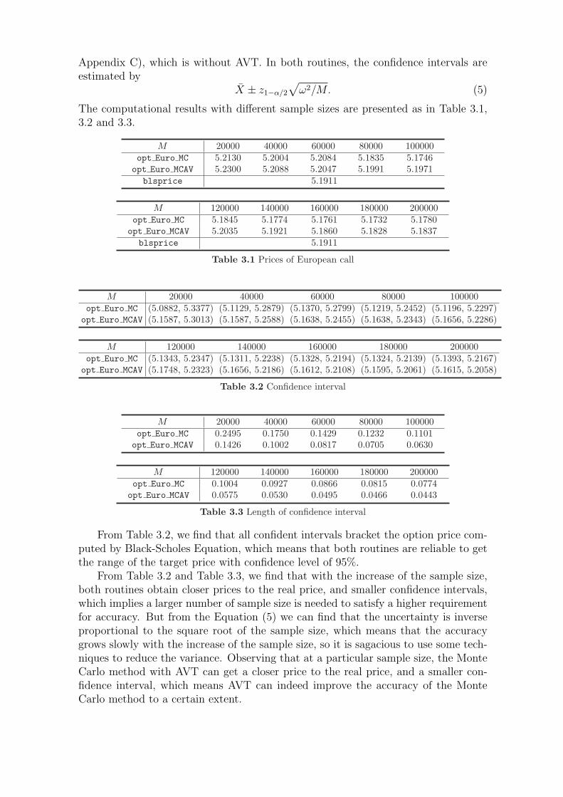
The computational results with different sample sizes are presented as in Table 3.1,3.2 and 3.3.

M 20000 40000 60000 80000 100000opt Euro MC 5.2130 5.2004 5.2084 5.1835 5.1746

opt Euro MCAV 5.2300 5.2088 5.2047 5.1991 5.1971blsprice 5.1911

M 120000 140000 160000 180000 200000opt Euro MC 5.1845 5.1774 5.1761 5.1732 5.1780

opt Euro MCAV 5.2035 5.1921 5.1860 5.1828 5.1837blsprice 5.1911

Table 3.1 Prices of European call

M 20000 40000 60000 80000 100000opt Euro MC (5.0882, 5.3377) (5.1129, 5.2879) (5.1370, 5.2799) (5.1219, 5.2452) (5.1196, 5.2297)

opt Euro MCAV (5.1587, 5.3013) (5.1587, 5.2588) (5.1638, 5.2455) (5.1638, 5.2343) (5.1656, 5.2286)

M 120000 140000 160000 180000 200000opt Euro MC (5.1343, 5.2347) (5.1311, 5.2238) (5.1328, 5.2194) (5.1324, 5.2139) (5.1393, 5.2167)

opt Euro MCAV (5.1748, 5.2323) (5.1656, 5.2186) (5.1612, 5.2108) (5.1595, 5.2061) (5.1615, 5.2058)

Table 3.2 Confidence interval

M 20000 40000 60000 80000 100000opt Euro MC 0.2495 0.1750 0.1429 0.1232 0.1101

opt Euro MCAV 0.1426 0.1002 0.0817 0.0705 0.0630

M 120000 140000 160000 180000 200000opt Euro MC 0.1004 0.0927 0.0866 0.0815 0.0774

opt Euro MCAV 0.0575 0.0530 0.0495 0.0466 0.0443

Table 3.3 Length of confidence interval

From Table 3.2, we find that all confident intervals bracket the option price com-puted by Black-Scholes Equation, which means that both routines are reliable to getthe range of the target price with confidence level of 95%.

From Table 3.2 and Table 3.3, we find that with the increase of the sample size,both routines obtain closer prices to the real price, and smaller confidence intervals,which implies a larger number of sample size is needed to satisfy a higher requirementfor accuracy. But from the Equation (5) we can find that the uncertainty is inverseproportional to the square root of the sample size, which means that the accuracygrows slowly with the increase of the sample size, so it is sagacious to use some tech-niques to reduce the variance. Observing that at a particular sample size, the MonteCarlo method with AVT can get a closer price to the real price, and a smaller con-fidence interval, which means AVT can indeed improve the accuracy of the MonteCarlo method to a certain extent.

6

Problem 3.b (5 points)

In this problem, the payoff the European vanilla call at maturity is determinedby {

S(T ) − K if K ≤ S(T ) ≤ Sb,

0 otherwise;(6)

where Sb = 70 and other parameters are the same as the previous problem. Forimplementation, it is exactly same as the previous one except calculating the payoff atmaturity by (6). Matlab routines opt EuroVanilla MCAV and opt EuroVanilla MC

are made (see Appendix D and E), and the results are listed as follows.

M 20000 40000 60000 80000 100000opt EuroVanilla MC 2.4295 2.4685 2.4876 2.4818 2.4865

opt EuroVanilla MCAV 2.4798 2.4865 2.4876 2.4876 2.4962



Table 3.4 Prices of European call with truncated payoff

M 20000 40000 60000 80000 100000opt EuroVanilla MC (2.3692, 2.4898)(2.4254, 2.5116)(2.4522, 2.5229)(2.4512, 2.5123)(2.4591, 2.5138)

opt EuroVanilla MCAV(2.4440, 2.5156)(2.4612, 2.5119)(2.4670, 2.5083)(2.4698, 2.5055)(2.4802 ,2.5122)

M 120000 140000 160000 180000 200000opt EuroVanilla MC (2.4635, 2.5135)(2.4692, 2.5155)(2.4720, 2.5153)(2.4727, 2.5135)(2.4696, 2.5082)

opt EuroVanilla MCAV(2.4832, 2.5125)(2.4906, 2.5177)(2.4907, 2.5160)(2.4905, 2.5144)(2.4890, 2.5116)

Table 3.5 Confidence interval





Table 3.6 Length of confidence interval

7

Problem 3.c (5 points)

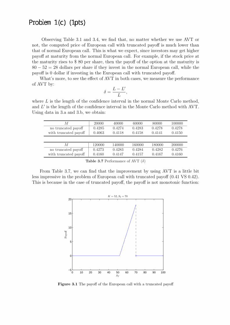
Observing Table 3.1 and 3.4, we find that, no matter whether we use AVT ornot, the computed price of European call with truncated payoff is much lower thanthat of normal European call. This is what we expect, since investors may get higherpayoff at maturity from the normal European call. For example, if the stock price atthe maturity rises to $ 80 per share, then the payoff of the option at the maturity is80 − 52 = 28 dollars per share if they invest in the normal European call, while thepayoff is 0 dollar if investing in the European call with truncated payoff.

What’s more, to see the effect of AVT in both cases, we measure the performanceof AVT by:

δ =L − L′

L,

where L is the length of the confidence interval in the normal Monte Carlo method,and L′ is the length of the confidence interval in the Monte Carlo method with AVT.Using data in 3.a and 3.b, we obtain:

M 20000 40000 60000 80000 100000no truncated payoff 0.4285 0.4274 0.4283 0.4278 0.4278

with truncated payoff 0.4063 0.4118 0.4158 0.4141 0.4150

M 120000 140000 160000 180000 200000no truncated payoff 0.4273 0.4283 0.4284 0.4282 0.4276

with truncated payoff 0.4160 0.4147 0.4157 0.4167 0.4160

Table 3.7 Performance of AVT (δ)

From Table 3.7, we can find that the improvement by using AVT is a little bitless impressive in the problem of European call with truncated payoff (0.41 VS 0.42).This is because in the case of truncated payoff, the payoff is not monotonic function:

0 10 20 30 40 50 60 70 80 90 100−5

0

5

10

15

20K = 52, Sb = 70

ST

Pay

off

Figure 3.1 The payoff of the European call with a truncated payoff

8

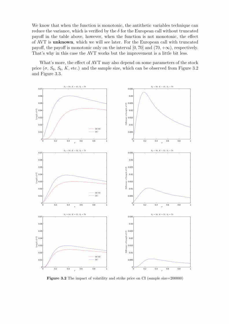
We know that when the function is monotonic, the antithetic variables technique canreduce the variance, which is verified by the δ for the European call without truncatedpayoff in the table above, however, when the function is not monotonic, the effectof AVT is unknown, which we will see later. For the European call with truncatedpayoff, the payoff is monotonic only on the interval [0, 70] and (70, +∞), respectively.That’s why in this case the AVT works but the improvement is a little bit less.

What’s more, the effect of AVT may also depend on some parameters of the stockprice (σ, S0, Sb, K, etc.) and the sample size, which can be observed from Figure 3.2and Figure 3.3.

0 0.2 0.4 0.6 0.8 10

0.01

0.02

0.03

0.04

0.05

0.06

0.07S0 = 50, K = 45, Sb = 70

σ

Leng

thof

CI

MCAVMC

0 0.2 0.4 0.6 0.8 10

0.005

0.01

0.015

0.02

0.025

0.03

0.035S0 = 50, K = 45, Sb = 70

σ

Diff

eren

ceof

Leng

thof

CI

0 0.2 0.4 0.6 0.8 10

0.01

0.02

0.03

0.04

0.05

0.06

0.07S0 = 50, K = 52, Sb = 70

σ

Leng

thof

CI

MCAVMC

0 0.2 0.4 0.6 0.8 10

0.005

0.01

0.015

0.02

0.025

0.03

0.035S0 = 50, K = 52, Sb = 70

σ

Diff

eren

ceof

Leng

thof

CI

0 0.2 0.4 0.6 0.8 10

0.01

0.02

0.03

0.04

0.05

0.06

0.07S0 = 50, K = 55, Sb = 70

σ

Leng

thof

CI

MCAVMC

0 0.2 0.4 0.6 0.8 10

0.005

0.01

0.015

0.02

0.025

0.03

0.035S0 = 50, K = 55, Sb = 70

σ

Diff

eren

ceof

Leng

thof

CI

Figure 3.2 The impact of volatility and strike price on CI (sample size=200000)

9

0 0.5 1 1.5 2

x 105

0

0.1

0.2

0.3

0.4

0.5

0.6

0.7

0.8

0.9S0 = 50, K = 45, Sb = 70

σ

Leng

thof

CI

MCAVMC

0 0.5 1 1.5 2

x 105

0

0.05

0.1

0.15

0.2

0.25

0.3

0.35S0 = 50, K = 45, Sb = 70

σ

Diff

eren

ceof

Leng

thof

CI

0 0.5 1 1.5 2

x 105

0

0.1

0.2

0.3

0.4

0.5

0.6

0.7

0.8

0.9S0 = 50, K = 52, Sb = 70

σ

Leng

thof

CI

MCAVMC

0 0.5 1 1.5 2

x 105

0

0.05

0.1

0.15

0.2

0.25

0.3

0.35S0 = 50, K = 52, Sb = 70

σ

Diff

eren

ceof

Leng

thof

CI

0 0.5 1 1.5 2

x 105

0

0.1

0.2

0.3

0.4

0.5

0.6

0.7

0.8

0.9S0 = 50, K = 55, Sb = 70

σ

Leng

thof

CI

MCAVMC

0 0.5 1 1.5 2

x 105

0

0.05

0.1

0.15

0.2

0.25

0.3

0.35S0 = 50, K = 55, Sb = 70

σ

Diff

eren

ceof

Leng

thof

CI

Figure 3.3 The impact of sample size and strike price on CI (σ = 0.4)

From Figure 3.1, when S0 = 50, Sb = 70, r = 0.1, and sample size M = 200000are fixed, for European call with a truncated payoff, we can find:

1. As long as the volatility of the stock price and the strike price are fixed, MonteCarlo method with AVT always get a smaller confidence interval than Monte Carlomethod without AVT. This implies that means AVT improves the accuracy to a cer-tain extent.

2. For both of these two Monte Carlo methods, with the increase of the volatilityof the stock price, the length of confidence interval goes up rapidly to a particularpeak, and then goes down slowly. This implies that Monte Carlo method with AVTis more accurate when the volatility of stock price is small.

3. Compared with Monte Carlo method without AVT, the confidence interval

10

changes less acutely in Monte Carlo method with AVT. This implies that the volatil-ity has less impact on Monte Carlo method with AVT.

4. No matter what the volatility of the stock price is, when the strike price goesup, the length of confidence interval decreases in both of these two Monte Carlo meth-ods. This implies that the higher the strike price is, the more accurate option pricesthese two Monte Carlo methods will get.

5. With the increase of the volatility of the stock price, the difference of confi-dence interval between these two methods first goes up from around 0 to a particularpeak, then goes down to less than 0.005. This implies that when the volatility ofthe stock price is too small or too large, AVT will not improve Monte Carlo methodimpressively.

6. No matter what the volatility of the stock price is, when the strike price goesup, the difference of confidence interval between these two methods decreases. Thisimplies the lower the strike price is, the more impressively that AVT improves MonteCarlo method.

From Figure 1.2, when S0 = 50, Sb = 70, r = 0.1, and σ = 0.4 are fixed, forEuropean call with a truncated payoff, we can find:

1. As long as the sample size and the strike price are fixed, Monte Carlo methodwith AVT always get a smaller confidence interval than Monte Carlo method withoutAVT. This implies that means AVT improves the accuracy to a certain extent.

2. For both of these two Monte Carlo methods, with the increase of the samplesize, the length of confidence interval goes down rapidly first, then goes down veryslowly. This implies that although increasing the sample size can improve the accu-racy, it is not necessary to use a huge sample (say sample size of 1000000). For thisproblem, 50000 is an appropriate sample size.

3. Compared with Monte Carlo method without AVT, the confidence intervalchanges less acutely in Monte Carlo method with AVT. This implies that the samplesize has less impact on Monte Carlo method with AVT.

4. No matter what the sample size is, when the strike price goes up, the length ofconfidence interval decreases in both of these two Monte Carlo methods. This impliesthat the higher the strike price is, the more accurate option prices these two MonteCarlo methods will get.

5. With the increase of the volatility of the stock price, the difference of con-fidence interval between these two methods first goes down very rapidly, then goesdown very slowly. This implies that although a larger sample will enhance the supe-riority of AVT, is not sagacious to use a huge sample (say sample size of 1000000).For this problem, 50000 is an appropriate sample size.

6. No matter what the sample size is, when the strike price goes up, the differenceof confidence interval between these two methods decreases. This implies the lowerthe strike price is, the more impressively that AVT improves Monte Carlo method.

Last but not least, although AVT reduces the sample variance when the func-tion of ε is monotonic, it may be a backfire when the function of ε is not monotonic.This can be proved as follows.

Considering continuous function X = X(ε), where ε ∼ N(0, 1), so X is a randomvariable. Let X̄ be the sample mean of X without using AVT, and X̄AV be the sample

11

mean of X with using AVT.If we do not use AVT, we can generate the following random series:

{ε1, . . . , εn, . . . , ε2n},where εi ∼ N(0, 1), i = 1, . . . , 2n and they are independent. Then

X̄ =

2n∑i=1

X(εi)

2n.

If using AVT, we need to generate

{ε1, . . . , εn,−ε1, . . . ,−εn},where εi ∼ N(0, 1), i = 1, . . . , n and they are independent. And

X̄AV =X̄1 + X̄2

2,

where

X̄1 =

n∑i=1

X(εi)

n, X̄2 =

n∑i=1

X(−εi)

n.

Therefore,

X̄AV =

n∑i=1

X(εi) +n∑

i=1

X(−εi)

2n.

Computing the variance of X̄ and X̄AV relatively:

V ar[X̄] = V ar

⎡⎢⎢⎣

2n∑i=1

X(εi)

2n

⎤⎥⎥⎦ .

Since εi, i = 1, . . . , 2n are independent and X(ε) is continuous, then X(εi), i =1, . . . , 2n are independent. Thus

V ar[X̄] =1

4n2

2n∑i=1

V ar[X(εi)].

Because εi, i = 1, . . . , 2n are also subject to a same distribution. Let σ∗ = V ar[X(εi)]X(εi), i = 1, . . . , 2n, then

V ar[X̄] =1

2nσ∗.

For X̄AV ,

V ar[X̄AV ] = V ar

⎡⎢⎢⎣

n∑i=1

X(εi) +n∑

i=1

X(−εi)

2n

⎤⎥⎥⎦

=1

4n2V ar

[n∑

i=1

X(εi) +n∑

i=1

X(−εi)

]

12

Considering εi and εj are independent for i �= j, thus

Cov(X(εi), X(εj)

)= 0, ∀i �= j,

Cov(X(εi), X(−εj)

)= 0, ∀i �= j,

then

V ar[X̄AV ] =1

4n2

{n∑

i=1

V ar[X(εi)] +n∑

i=1

V ar[X(−εi)] + 2n∑

i=1

Cov(X(εi), X(−εi)

)}

Since εi ∼ N(0, 1), then −εi ∼ N(0, 1), indicating X(εi) and X(−εj) are subject tothe same distribution for all i and j. Therefore,

V ar[X̄AV ] =1

4n2

{2nσ∗ + 2

n∑i=1


)}

=σ∗

2n+

1

2n2

n∑i=1


).

Then

V ar[X̄] − V ar[X̄AV ] = − 1

2n2

n∑i=1


).

If x(ε) is monotonic increasing / decreasing, we have shown in Problem 1 that


)< 0.

Therefore, when X(ε) is monotonic,

V ar[X̄] − V ar[X̄AV ] > 0,

which means AVT reduces the sample variance. However, if X(ε) is not monotonic,for example X = ε2, the following will be true:

εi ↑{

X(εi) ↑, X(−εi) ↑ εi > 0

X(εi) ↓, X(−εi) ↓ εi < 0

εi ↓{

X(εi) ↓, X(−εi) ↓ εi > 0

X(εi) ↑, X(−εi) ↑ εi < 0

which meansCov

(X(εi), X(−εi)

)> 0,

This leads toV ar[X̄] − V ar[X̄AV ] < 0.

In this case, AVT increases the sample variance.

13

Question 2(5 pts)

”1 day 95% VaR for the portfolio in Microsoft is $500,000” means:” We are 95%

certain that we will not lose more than $500,000 dollars in the next 1 day”.

The advantage of VaR:

1, Simple: It provides a single number to summarize the total risk in a portfolio of

financial assets.

2, Intuitive: To ask ”how bad can things get”

3, Monitoring: easy to control and monitor the risk excesses by portfolio and by business

against approved limits.

Disadvantage of VaR: Risk is usually multi-dimensional and has heavy-tail, one number

cannot exactly describe the risk profiles and captures certain key risk factors.

(b) For stock A:

σday = 0.12, N = 1, X = 99, N(−2.33) = 0.01

The size of the position is $1,000,000

so the standard deviation of the change is:

$1, 000, 000 ∗ 0.12 = $12, 000

The 1-day 99% VaR is :

$12, 000 ∗ 2.33 = $27, 960

The 10-day %99 VaR is:

$27, 960 ∗√

10 = $88, 417

1

tailang

文本框

(a)

function [price, CI] = opt_Euro_MC(S0, K, r, T, sigma, type, N, alpha)%**************************************************************************% METHOD: basic Monte Carlo Method for basic European option%**************************************************************************% INPUT:

% type = 1: put option.

% alpha: 1 - alpha is the confidence level (optional).%**************************************************************************% OUTPUT:

% CI: confidence interval.%**************************************************************************

if nargin < 8% default confidence level

end

randn('seed'if type == 0 % compute price of call option PriceVector = exp(- r * T) * max(0, S0 * exp((r - 0.5 * sigma ^ 2)...

else % compute price of put option PriceVector = exp(- r * T) * max(0, K - S0 * exp((r - 0.5 * ...

end

% compute the confidence interval

Appendix B MALAB code for MC Method for pricingEuropean call

function [price, CI] = opt_Euro_MCAV(S0, K, r, T, sigma, type, N, alpha)%**************************************************************************% METHOD: Monte Carlo Method With antithetic variable techniques for basic% European option%**************************************************************************% INPUT:




if nargin < 8% default confidence level: 0.95

end

randn('seed' % generate two random matrice

if type == 0 % compute price of call option PriceVector1 = exp(- r * T) * max(0, S0 * exp((r - 0.5 * sigma ^ 2) * T + sigma *

PriceVector2 = exp(- r * T) * max(0, S0 * exp((r - 0.5 * sigma ^ 2) * T + sigma *

else % compute price of put option PriceVector1 = exp(- r * T) * max(0, K - S0 * exp((r - 0.5 * sigma ^ 2) * T + sigma

PriceVector2 = exp(- r * T) * max(0, K - S0 * exp((r - 0.5 * sigma ^ 2) * T + sigma

end


Appendix C MALAB code for MC Method with antitheticvariable technique for pricing European call

function [price, CI] = opt_EuroVanilla_MC(S0, K, r, T, sigma, Sb, type, N, alpha)%**************************************************************************% METHOD: basic Monte Carlo Method for basic European option with a % truncated payoff%**************************************************************************% INPUT:





end

randn('seed'PriceStock = S0 * exp((r - 0.5 * sigma ^ 2) * T + sigma ...

if type == 0 % compute price of call option


else % compute price of put option disp('payoff not defined')end

Appendix D MALAB code for MC Method for pricingEuropean call with truncated payoff

function [price, CI] = opt_EuroVanilla_MCAV(S0, K, r, T, sigma, Sb, type, N, alpha)%**************************************************************************% METHOD: Monte Carlo Method with antithetic variable techniques for % European option with a truncated payoff%**************************************************************************% INPUT:





end

randn('seed' % generate two random matrice

PriceStock1 = S0 * exp((r - 0.5 * sigma ^ 2) * T + sigma ...

PriceStock2 = S0 * exp((r - 0.5 * sigma ^ 2) * T + sigma ...

if type == 0 % compute price of call option


else % compute price of put option disp('payoff not defined'end

Appendix E MALAB code for MC Method with antithetic variabletechnique for pricing European call with truncated payoff

Sol2 math6911 w07 - YorkU Math and Statshmzhu/Math-4143/assignments/Solution3/solution… · lim M...

Documents

Transcript of Sol2 math6911 w07 - YorkU Math and Statshmzhu/Math-4143/assignments/Solution3/solution… · lim M...