1

Project Number: LDA-1006

Project Number: MT- 1003

Soil Reinforcement with Natural Fibers for Low-Income Housing Communities

A Major Qualifying Project

Submitted to the Faculty of

WORCESTER POLYTECHINIC INSTITUTE

In partial fulfillment of the requirement for the

Degree of Bachelor of Science

By

_________________________

Bryan Gaw

_________________________

Sofia Zamora

Approved by:

________________________

Professor Leonard D. Albano, Advisor

_______________________

Professor Mingjiang Tao, Co-Advisor

2

Abstract

The objective of this project is to identify a natural fiber to enhance the shear strength

and bearing capacity of a cohesive soil. This study includes a proposed protection method to

increase the durability of the selected fiber, determination of the optimum reinforcement

scheme in terms of fiber’s content and length, and investigation of the reinforced soil through

laboratory experiments on footing bearing capacity and slope stability analysis.

3

Acknowledgements

We would like to thank the following people for their role in helping make this project a

success:

Don Pellegrino - Laboratory Manager

Dean Daigneault – Laboratory Manager

Leonard Albano – Associate Professor of Civil and Environmental Engineering

Mingjiang Tao – Assistant Professor of Civil and Environmental Engineering

4

Authorship Page

This report was authored by the following individuals, each had specific authorship

responsibilities and each collaborated between disciplines across the completion of the project.

Bryan Gaw ______________________________

- Selection of protection method.

- Testing implementation.

- Preparation of test specimens and testing.

- Co-analyzing data.

- Authorship of Background and Methodology.

- Editing.

Sofia Zamora ______________________________

- Selection of reinforcement method and natural fiber.

- Planning of experimental implementation.

- Design of special devices for tests.

- Preparation of test specimens and testing.

- Co-analyzing data.

- Modeling and analysis of implementation.

- Cost estimation.

- Authorship of Introduction, Analysis and Results and Applications Chapters.

- Formatting and editing.

5

Capstone Design Statement

The capstone design criteria aim towards driving the students through a decision making

process where the solution to a problem is developed though synthesis and analysis of different

aspects that shape the final solution design. The main eight realistic constraints that shaped the

design process during this project are the following: economic, environmental, sustainability,

constructability, ethical, health and safety, social and political.

The economic and social constraints were the leading aspects in the design of the

project. The social constraint determined the population we aimed to provide a solution for.

We are aware of the large disparity among social classes in developing countries and the low

living standards this brings to the poorest communities; therefore we decided to focus on the

poorest social groups in these countries. Our main concern is the high-risk conditions in which

these communities develop their housing. The project focuses on beginning to develop a

solution for these communities to establish on hillsides under safer conditions. We determined

the improvement of safety required the stabilization of the ground to be developed.

The scarcity of resources available to these communities made the economic constraint the

leading criteria in the selection of the soil reinforcement method. We evaluated different

reinforcing methods and selected the most feasible one for these communities. Therefore we

studied a method that properly reinforced a cohesive soil type, commonly encountered in

developing nations and that required inexpensive, locally attainable materials and minimal

construction effort and machinery.

The environmental and sustainability constraints were also part of the core design. The

environmental constraint determined the materials and process used for the reinforcement

method. We selected natural fibers, and used a 100% natural protection method for the

selected fiber, because we wanted to prevent contaminating the soil with detrimental

materials. Following the environmental concept of reducing drastic modifications to the

landscape as to not disrupt the existing ecosystem, we aimed to sufficiently increase the shear

strength of the soil in the slope to minimize the grading process and the change in runoff. The

sustainability constraint determined our design approach. Our design aimed to provide a

6

reinforcement method which at the end of its useful life would become an asset to the soil

while allowing other stability methods to come in place. Therefore we selected biodegradable

materials which will not endanger the species or the type of organisms that inhabit in the area.

The key aspect of the design became to provide a temporary solution while a more permanent

but equally sustainable solution could be implemented. An example of such a method is

planting a specific species of tree capable of growing strong widespread roots during the

lifespan of the fiber reinforcement. The roots of the trees only need to hold the upper 3 or 4

feet of soil. The design aims to behave as an item in a closed ecosystem cycle.

The constructability constrains the manner how the fibers would be implemented. We

evaluated the construction resources available to the target-users and we determined the most

feasible implementation would be by mixing the fibers into the soil instead of inserting layers of

fiber fabric or ties. We evaluated the difficulties of the soil removal, fiber preparation, and soil

mixing and compaction and provided a basic cost and schedule estimate. We designed a basic

reinforcing method through the modeling of grading, soil compaction and basic drainage. The

models evaluate the increment in factor of safety of the slope when the reinforcement is in

place. The models were modified iteratively aiming to minimize the required depth of

reinforcement while the increase of factor of safety remained acceptable.

The health and safety constraint shaped the criteria by which the reinforcement method

was deemed successful. The fibers and the components of the protective coating were selected

based on their toxicity reports. All of the materials are non-toxic. Also, as described in the

previous paragraph, the reinforcement models were deemed successful when they had a factor

of safety larger than 1.1. This extra 0.1 accounted for the peak load concentrations that could

occur during the construction process. The design of the bearing capacity test and the models,

were done in compliance with the safe dimensions dictated in the Central American Building

Code,1996 .

The political constraint dictated the Construction Manuals and Building Codes that were

consulted in order to comply with the construction practices allowed in the focus areas. Also, in

7

recognition of the political atmosphere in these communities, we simplified the communal

decisions and collective work required for the implementation of the reinforcement.

The ethical constraint lead to us to complete this project according to Code of Ethics for

Engineers, 2003. According to the 6th Fundamental Canon, we conducted ourselves honor ably,

responsibly, ethically, and lawfully so as to enhance the honor, reputation, and usefulness of

the profession. We determined our conclusions and recommendations according to the

Professional Obligations One and Two.

8

Table of Contents Abstract ........................................................................................................................................... 2

Acknowledgements ......................................................................................................................... 3

Authorship Page .............................................................................................................................. 4

Capstone Design Statement ........................................................................................................... 5

List of Figures ................................................................................................................................ 10

List of Tables ................................................................................................................................. 12

Chapter 1: Introduction ................................................................................................................ 14

Chapter 2: Background ................................................................................................................. 19

Current Soil Stabilization Technologies ..................................................................................... 20

Effect of Soil-Fiber Reinforcement on Soil Shear Strength ....................................................... 25

Important Impact of Soil-Fiber Reinforcement: Improvement of Soil Bearing Capacity ......... 27

Chapter 3: Methodology ............................................................................................................... 31

Selection of Fiber and Experimental Design Parameters .......................................................... 31

Selection of Testing Sequence and Procedures ........................................................................ 32

Soil Selection ............................................................................................................................. 35

Soil Synthesis ............................................................................................................................. 38

Fiber Preparation ...................................................................................................................... 41

Testing ....................................................................................................................................... 44

1. Tensile Strength Test of Coconut Fiber .......................................................................... 44

2. Proctor Compaction Test ............................................................................................... 45

3. Shear Strength Test ........................................................................................................ 47

4. Indirect Tensile Strength Test ........................................................................................ 50

5. Bearing Capacity Test ..................................................................................................... 52

Modeling of Slope Stability with Soil Fiber Reinforcement ...................................................... 59

Chapter 4: Results and Analysis of Testing ................................................................................... 63

Particle Distribution of the Soil ................................................................................................. 63

Tensile Strength Test of Fibers .................................................................................................. 66

Proctor Compaction Test .......................................................................................................... 68

Unconfined Compression Test .................................................................................................. 69

9

Indirect Tensile Test .................................................................................................................. 83

Bearing Capacity Test ................................................................................................................ 85

Modeling of Slope Stability with Soil Fiber Reinforcement ...................................................... 89

Chapter 5: Implementation of Reinforcement in Low-Income Communities .............................. 91

Chapter 6: Conclusions and Recommendations ........................................................................... 97

Preparation of the fibers ........................................................................................................... 97

Testing Coated Fibers ................................................................................................................ 98

Mixing the fibers into the soil ................................................................................................... 98

Shear Strength Test ................................................................................................................... 99

Saturated Test ......................................................................................................................... 100

Bearing Capacity ...................................................................................................................... 100

Modeling of Slope Stability with Soil Fiber Reinforcement .................................................... 101

Bibliography ................................................................................................................................ 102

Appendix A .................................................................................................................................. 106

Devastating Effects of Natural Disasters on Low Income Settlements ................................... 106

Appendix B .................................................................................................................................. 110

Practices in Adobe Construction ................................................................................................. 110

Appendix C .................................................................................................................................. 113

Proctor Compaction Test Procedures and Results .................................................................. 113

Appendix D .................................................................................................................................. 115

Sample Data Tables per UCT sample and Stress-Strain Curves per UCT specimen. ............... 115

0.8% 35 mm ......................................................................................................................... 115

0.8% 50 mm ......................................................................................................................... 119

1.8% 35 mm ......................................................................................................................... 124

Appendix E .................................................................................................................................. 129

Results of Statistical T-Test ..................................................................................................... 129

Appendix F: Proposal .................................................................................................................. 130

Abstract ................................................................................................................................... 131

Introduction and Problem Statement ..................................................................................... 133

10

Scope of Work ......................................................................................................................... 137

Capstone Design ...................................................................................................................... 140

Methodology ........................................................................................................................... 143

List of Figures

Figure 1: Types of landslide movements. Copyright Geosciences Australia ................................ 19

Figure 2: Bishop's Method. Copyright Tsushida, 2002. ................................................................ 21

Figure 3: Distribution of stresses in SWR ...................................................................................... 23

Figure 4: Date Palm Study 40 mm CBR Results. Copyright Marandi, 2008. ................................. 26

Figure 5: Load-penetration curves for varying reinforcement content. Copyright Yetimoglu,

2004 .............................................................................................................................................. 27

Figure 6: Zones evaluated in Terzaghi's Bearing Capacity Theory. Copyright CE-REF.com. ........ 28

Figure 7: Typical low income adobe house in Rio de Janeiro. Copyright VIVERCIDADES, 2006) . 36

Figure 8: Taxonomy Soil Classification Pyramid. Copyright NRCS, 2009. ..................................... 37

Figure 9A: WPI Sand Sieve Analysis. Figure 9B: Weighing of the Soil

Materials for Mixing ...................................................................................................................... 40

Figure 10: Comparison of fiber dimensions with a dime. ............................................................. 41

Figure 11: Complete mix of coating .............................................................................................. 42

Figure 12: Fiber cutting process .................................................................................................... 43

Figure 13: Preparation of coated-fiber samples for Ultimate Tensile Test. ................................. 44

Figure 14: PCT Fiber Reinforced Mold .......................................................................................... 46

Figure 15: Adding fibers to the soil. .............................................................................................. 47

Figure 16: 20% MC Reinforced Soil Sample Preparation .............................................................. 47

Figure 17: Placing an UCT sample ................................................................................................. 49

Figure 18A: Non-Reinforced Failure Figure 18B: 3.2% Reinforced Failure ............... 50

Figure 19: ITT sample loading. ...................................................................................................... 51

Figure 20A: Non-reinforced ITT Failure Figure 20B: 1.8% ITT Failure Figure

20C: 2.4% ITT Failure ..................................................................................................................... 52

11

Figure 21: Typical dimensions of low income housing ................................................................. 53

Figure 22: 1 ft long housing strip footing ...................................................................................... 54

Figure 23: Scaled down footing .................................................................................................... 57

Figure 24: Bearing Capacity Test Box ............................................................................................ 57

Figure 25A: Bearing Capacity Test Figure 25B: Failed reinforced soil ................................. 59

Figure 26: Proposed configuration for development. .................................................................. 60

Figure 27: STB Software Input Values ........................................................................................... 62

Figure 28: 37% or 20 degree- slope .............................................................................................. 62

Figure 29: 47% or 25 degree-slope ............................................................................................... 62

Figure 30: 70% or 35 degree-slope .............................................................................................. 62

Figure 31: 84% or 40 degree-slope ............................................................................................... 62

Figure 32: Particle Distribution Graph Ideal vs. WPI Sand ............................................................ 64

Figure 33: Tropical Soil Particle Distribution ................................................................................ 65

Figure 34: 10-Fiber Tensile Test Load vs. Extension Graph .......................................................... 66

Figure 35: Proctor Compaction Test Results................................................................................. 68

Figure 36 A: Non-reinforced B: 0.8% C: 1.8% D: 2.4% E: 3.2% F: Clumping behavior of soil

layers with 3.2% fiber content. ..................................................................................................... 71

Figure 37: Non-Fiber UCT Specimen 1 .......................................................................................... 72

Figure 38: Representation of soil re-compressive behavior through a spring ............................. 73

Figure 39: 1.8% 50 mm UCT True Stress-Strain Curve, Specimen # 2 .......................................... 74

Figure 40: 1.8% 50 mm UCT Eng. Stress-Strain Curve, Spec. # 2 .................................................. 74

Figure 41: Comparison of Maximum Shear Strength according to the different fiber content and

length combinations ..................................................................................................................... 77

Figure 42: Comparison of Maximum Shear Strength according to Fiber Length ......................... 78

Figure 43: Comparison of Maximum Shear Strength according to fiber % ................................. 79

Figure 44: Cube subjected to compressive and shear stresses. Li and Kapania, 2007. ................ 81

Figure 45: Generation of Mohr's Circle through the transformation equations for angles 0-360.

Li and Kapania, 2007. .................................................................................................................... 81

Figure 46: Mohr's Circle Model for Reinforced and Un-Reinforced Soil Samples. ....................... 82

12

Figure 47: Tensile Strength in PSI vs. Fiber % by weight .............................................................. 85

Figure 48: Un-reinforced Stress vs Settlement Curve................................................................... 86

Figure 49: Reinforced Soil: Stress vs Settlement Curve ................................................................ 87

Figure 50: 1:4 scaled down footing ............................................................................................... 88

Figure 51: 1:4 Scale Stress-Strain Curve. Results of Reinforced and Un-reinforced soils. ........... 88

Figure 52: Slope angle vs Factor of Safety % Improvement. ........................................................ 90

Figure 53: Current Construction Methods in Low-Income Communities .................................... 92

Figure 54: Slope Grading Method for 25 degrees ........................................................................ 93

Figure 55: Required Grading Process for 40 degrees. .................................................................. 93

Figure 56: Drainage System Suggestion ........................................................................................ 95

List of Tables

Table 1: Testing Procedures .......................................................................................................... 34

Table 2: Optimum soil for Adobe composition ............................................................................. 36

Table 3: Ranges of soil percentages by weight for sandy loam .................................................... 37

Table 4: Lbs of soil required per set of tests ................................................................................. 38

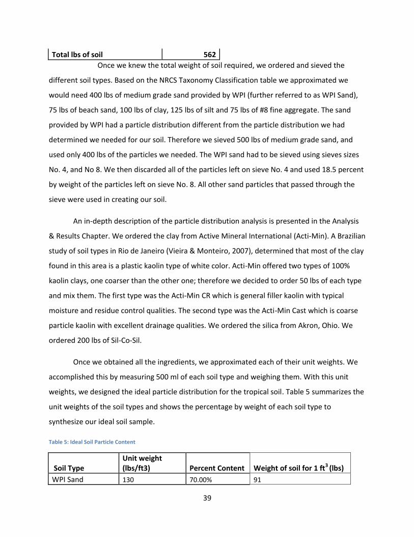
Table 5: Ideal Soil Particle Content ............................................................................................... 39

Table 6: Actual Soil Type Content ................................................................................................. 40

Table 7: Lbs of Coated Fiber required per set of tests.................................................................. 43

Table 8: UCT Specimens ................................................................................................................ 48

Table 9: Loading from Central American Building Code ............................................................... 54

Table 10: Ultimate Load Calculations ........................................................................................... 54

Table 11: Calculations ................................................................................................................... 57

Table 12: Vesic's Shape Factors .................................................................................................... 58

Table 13: Particle Distribution of Ideal Sand ................................................................................ 63

Table 14: Particle Distribution of WPI Sand .................................................................................. 64

Table 15: Fiber Ultimate Tensile Strength Test Results ................................................................ 67

Table 16: UCT Data Sample Calculation ........................................................................................ 69

Table 17: UCT Data Sample Calculation ........................................................................................ 70

13

Table 18: Peak Stress Summary Table .......................................................................................... 75

Table 19: Table summarizing ANOVA Comparisons ..................................................................... 76

Table 20: ANOVA Comparison 1 ................................................................................................... 77

Table 21: ANOVA Comparison 2 ................................................................................................... 78

Table 22: ANOVA Comparison 3 ................................................................................................... 79

Table 23: Mean shear stress per reinforcement combination ..................................................... 80

Table 24: T-Test results ................................................................................................................. 80

Table 25: Indirect Tensile Test results .......................................................................................... 83

Table 26: ANOVA results for IIT .................................................................................................... 84

Table 27: Modeling Results ........................................................................................................... 89

Table 28: Estimated costs for a 40 ft x 20 ft area stabilization. .................................................... 96

14

Chapter 1: Introduction

Currently 1.4 billion people live below the international poverty line of $1.25 income per

day. Many social problems that currently affect the world are caused by poverty, which causes

the deficient access to basic needs for many humans. This is reflected by the frequent

occurrence of disasters in low income housing settlements. The most common are (UNEP,

1996):

Fires: Necessity does not allow most low income housing around the world to follow fire

protection precautions.

Floods: Deficient resources do not allow for proper planning, which results in inadequate

draining facilities.

Earthquakes: Non-engineered construction does not include a horizontal resistant frame

that can withstand seismic forces which results in the collapse of the structures.

Landslides: Low income communities in developing countries tend to build their housing in

landslide prone hillsides.

The problems developed by poverty can be summarized into: political and economical

instability, social and economic dependency and low living standards and access to basic needs

(Shah [1], 2009).

The disaster that has been minimally addressed for low income settlements is landslides on

hillsides. As previously mentioned, the countries with the highest frequency of landslide

disasters are the developing nations. These nations have large communities with minimal

resources which need to settle on high risk hillsides in order to have access to the cities with

the highest employment resources. Additionally, these countries are divided by their high

educational disparity, which doesn’t allow the least educated groups to understand and

evaluate the consequences of unsustainable development practices (Sassa & Canuti, 2008).

Examples of these activities are clearing the vegetative cover in order to grow crops, livestock

and developing settlements on hillsides without adequate environmental planning. This

inadequate planning does not allow enough water to reach the groundwater table which

15

creates drastic drops in its levels, weakening the soil. Other effects are the erosion of the soil

caused by excessive runoff and the addition of significant weight to the running material due to

the accumulation of large amounts of water in between houses (Alexander, 1992). These

populations not only develop housing settlements in ways that leave the soil completely

unprotected but they also build houses right on the slope border. This causes an extreme

burden on the shear strength of the soil in the hillside increasing the probability of landslide

occurrence.

For instance, in 1999 an abrupt landslide occurred in Vargas State, Venezuela, causing a

disaster known as the Tragedy of Vargas. Vargas State is one of the poorest states in the

country, with many settlements on hillsides with poor development practices. This reflected on

the tragedy killing tens of thousands of people and destroying thousands of homes, causing the

complete collapse of the state’s infrastructure. The gigantic mudslides were triggered by the

rainfall of a strong tropical storm (Venezuelan Government, 2007). Another country where

landslides have had disastrous effects on hillside settlements is Brazil. Brazil is an ideal sample

location around which to focus a case study because the Brazilian government has very in-

depth records about landslide disasters and shares similar social and topographical

characteristics with most developing countries.

The area with the most frequent landslides occurrence within Brazil is Serra do Mar, a

long coast range that runs from the south to the southeastern regions of the country. Due to

the low costs of establishing housing in unwanted territories, many settlements were built

upon the hillsides in and around cities along Serra do Mar, since the 1960’s. These communities

are internationally known as the slums of Rio de Janeiro. Nowadays, these hillsides are densely

populated and the population’s unsustainable practices have increased the probability of slope

failure to occur. These conditions have caused the erosion of large amounts of soil, which has

significantly increased the occurrence of landslides (Fernandez, et. al, 2003). Please see

Appendix A for further details.

The soil at the base of the steep slopes in Rio de Janeiro is made of an upper layer of

clay soil with an approximate content of 40% clay which lies over a sandy silt saprolite soil

16

(Fernandez, et. al, 2003). This configuration has caused two main concerns among experts. The

first one is that clay soil significantly varies its moisture content because it holds moisture

according to the weather conditions. This can cause structures to sink when moisture content

decreases drastically and to crack when moisture content increases drastically. A way to avoid

this is through proper ground compaction, so the ground does not shift under the weight of the

home (Smith, 2007). The second concerning factor is the steepness of the hillsides on which

these settlements are constructed (Fernandez, et. al, 2003). A recent field study establishes

that the slope angles of the hills in Serra do Mar vary from 20: to 29: (Cruz O. and Colangelo,

2000). A study by Zhou, et al (2002) observed that landslide potential is very high for slopes

with threshold angles of 25˚ to 30˚ and a study by GAO (1993) presents that the landslide

potential increases rapidly for hill slopes above 31˚.

There are several methods for stabilizing shear strength of slopes, some of the most

common ones are:

Reinforcing compacted soil layers with steel wire mesh.

Reinforcing compacted soil layers with geo-synthetics.

Mixing lime with the soil.

Randomly mixing fibers into the soil.

Most of these methods require a lot of organization, planning, heavy machinery,

qualified workers and a high monetary investment; all resources to which these communities

do not have access to. We believe future development should be sustainable; therefore we

want to help produce a soil stabilization method that has a positive contribution on the

environment. Based on this idea and the resources the sample communities have available to

them, we determined the reinforcement method that aligns the most with our objectives is the

random mix of environmentally friendly fibers into the soil. Key concepts within the idea of

sustainability for this project are to use materials locally available to these communities and

minimally modify the landscape, which would decrease the required work effort.

17

Increasing the bearing capacity of the soil and the stability of soil in slopes are only two

applications of reinforcing the soil with fibers. The main effect of this reinforcement is the

increase of shear strength of the soil. Previous fiber soil reinforcement studies indicate that the

fibers significantly increase the shear strength of different types of soils in optimum conditions

(Wayne, 1988). According to Tezarghi’s and Vesic’s soil bearing capacity studies, the bearing

capacity of the soil has a direct relationship with the shear strength of the soil. In foundation

engineering the bearing capacity of the soil is defined as the maximum homogeneously

distributed pressure in direct contact, a soil can withstand before suffering shear failure.

Therefore an increase in the bearing capacity of the soil would allow the soil to hold a larger

load in the same area, which can prove useful in many aspects of housing development. Some

of these aspects are the ability to build larger structures, reduce the size of footings, and easily

stabilize soil for roads.

The goal of our project was to test the shear strength, tensile strength and bearing capacity

behavior of tropical soil reinforced with randomly mixed coir fiber. In order to accomplish this

goal we separated the required work into the following nine steps:

1. Select a fiber that is easily attainable to low income housing areas.

2. Emulate a soil where landslides have devastating effects on low income housing.

3. Determine the fiber treatment process and apply it.

4. Determine the properties of the treated and non-treated fiber through tensile strength

tests and measurements of the dimensions of the fibers.

5. Obtain the compaction parameters through the Proctor Compaction test.

6. Identify the optimal stabilization parameters: the fiber content and fiber length. Testing

procedures: Unconfined Compression Test (UCT), Indirect Tensile Test (ITT) and

Saturated Unconfined Compression Test (SUCT).

7. Determine the benefits obtained in the soil bearing capacity.

8. Determine the benefits from fiber reinforcement in slope stability.

9. Analyze the results and elaborate conclusions and recommendations.

18

Our Major Qualifying Project demonstrated how an easily attainable and inexpensive

material for low income communities worldwide could reinforce tropical soil to improve its

bearing capacity. The reinforcement parameters found in this study provide a good base for

future investigation and design of soil stabilization methods. The reinforcement benefits can be

extended to other construction fields.

19

Chapter 2: Background

A landslide is a mass movement of soil, debris or rocks down slope under the direct

influence of gravity (Cruden, 1991). Slope failure is the phenomenon that creates a landslide;

this occurs when the weight of the material on a slope exceeds the strength of the material that

composes the slope. The strongest determinant of the feasibility of a location to fail is its

topography: the angle and shear strength of the slope soil. The movement of materials in a

landslide can occur abruptly, or gradually and slowly. Figure 1 illustrates the different ways

landslides can occur: as a flow, slump, topple, slide, and creep or as a fall. Sudden events are

extremely dangerous because of the fast speed of the material and the momentum it carries.

Meanwhile gradual events might move only millimeters per year and remain active for long

periods. Even though this last type of landslide is not life-threatening it causes considerable

damage to structures (Geosciences Australia, 2009). We can conclude that the most dangerous

landslides are the ones that occur abruptly. Please refer to Appendix A for further detail.

Figure 1: Types of landslide movements. Copyright Geosciences Australia

20

One major problem that occurs frequently is the necessity of low-income families to

establish their residence on steep hillsides prone to landslides. Currently, most people that

move into these poor housing developments participate in unsustainable practices that

increase their risk. Most of these practices significantly increase the free-to-run weight of

materials laying on the hillside surface. Landslides occur when the stability of a slope changes

from a stable to an unstable condition. Currently, several stabilization methods are used to

increase the factor of safety in areas developed on steep hillsides. One of the easiest methods

to apply is the reinforcement of the soil with randomly mixed fibers. The stabilization is one of

the many impacts of this procedure. The main effect is an increase in the shear strength of the

soil. Laboratory tests were performed to determine the characteristics of the optimum

reinforcement and the benefits of the reinforcement on the soil shear strength and bearing

capacity. Additionally, a slope stability program was used to model the effect of the

reinforcement of a shallow soil layer on a hillside.

Current Soil Stabilization Technologies

The shear strength of a soil influences the stability of the structures it supports. The

shear strength, t (tau), of a soil is the internal resistance per unit area that a soil mass can

provide to resist failure and sliding along its plane. Most geotechnical failures involve a shear-

type failure which is determined by the nature of the soil. Soil is composed of individual

particles that slide when the soil is loaded. The characteristics of the different types of soil

particles and their proportions in the soil establish the amount of cohesion and friction

between particles. Mohr-Coulomb’s equation describes the relationship between shear

strength and normal stress, angle of friction and cohesion (Day, 1999):

𝑡 = 𝑐′ + 𝜎 ′ ∙ tan𝜃′ (1)

21

As Equation1 presents, the shear strength of a soil has a direct relationship to the soil

cohesion, c’, and angle of friction, θ’ (Izad, 2008). When the maximum shear resistance of a soil

is reached, the soil is regarded as having failed. The total stress on any plane can be determined

by the normal stress, σ’, which acts perpendicular to the surface and the shearing stress which

acts along the surface. The shear strength of a soil depends on its moisture content and its

compaction level.

A stable slope can be defined as a slope where the forces available to resist movement

within the soil are greater than the forces driving movement. Slope stability encompasses the

analysis of static and dynamic stability of embankments and natural slopes. In order to

establish the stability condition of a slope, the slope’s factor of safety is calculated. The factor

of safety is the ratio of the forces resisting movement to the forces driving movement. If the

factor of safety (FS) is equal or greater than 1, then the slope is stable, and if the factor of safety

is less than 1, then the slope is unstable. The planes along which the factor must be calculated

in slope stability analysis are usually irregular, which makes the process very complex. A

method for determining the factor of safety in a slope is Bishop’s Method (Coduto, 1998).

Figure 2: Bishop's Method. Copyright Tsushida, 2002.

22

The Simplified Bishop’s Method is a method for calculating the stability of slopes. The

method can produce factor of safety values within a few percent of the correct values. The

Simplified Bishop’s Method is as follows:

Where (2)

D is the effective cohesion

Φ is the effective internal angle of internal friction

b is the width of each slice

W is the weight of each slice

u is the water pressure at the base of each slice

α is the slope angle

Equation # 2 must be solved iteratively because it contains F on both sides of the

equation. Since the process to reach convergence can be long and tedious, several simple

programs exist to model Bishop’s method in different circumstances. According to this method

the failure occurs along a cylindrical slip surface generated by the rotation of a block of soil

around a center point O. The method obtains the factor of safety of the slip surface by

evaluating the whole system moment equilibrium about O. This is a simplified method because

all the inter-slice forces are assumed horizontal. Figure 2 illustrates Bishops’ analysis method.

Currently there are several methods to improve slope stability. We searched for a

method that could be implemented in our study area. This required that we focused on

methods that were relatively inexpensive and that required minimum machinery. The following

methods align the best with these requirements:

Steel wire reinforcement: This method consists of dividing the soil in compacted layers and

then reinforcing each layer with steel wire mesh. The forces that the mesh induces into the

soil depend on the mesh geometry, frictional characteristics, vertical soil pressure on the

strip, and strength and stiffness characteristics of the strip. The mesh should be designed to

23

include a layer of steel that will corrode during the expected life of the mesh preventing loss

of critical mesh cross-area. The durability of this soil reinforcement relies on the ability of

the mesh to retain a pre-established level of tensile strength. The following comparison

illustrates how the reinforcement works: Figure 3-A illustrates that if a vertical stress is

applied on unreinforced soil it deforms both laterally and vertically until it reaches a new

equilibrium. Figure 3-B illustrates that if a vertical stress is applied to a mass of soil

reinforced with metal sheets on planes perpendicular to the normal stress, the soil

deformations are constrained due to the interaction between the soil and the mesh.

Figure 3: Distribution of stresses in SWR

One of the advantages of using this method is that the construction materials are light,

easy to transport and quick to construct. Other advantages are the only machinery required

is a backhoe and a compactor, and it’s not extremely expensive. Disadvantages of this

method are that it cannot be implemented in soils with a high content of silt and clay, and it

is very difficult to apply it to extensive sloped areas. Another problem is that it has

detrimental impacts to the environment at the end of its useful life because the corroded

steel is toxic to the environment (Pereira, 1994).

Geo-synthetic reinforcement: This method consists of dividing the soil in compacted layers

and reinforcing each layer with geo-synthetics. The synthetics are used in two ways during

slope reinforcement. The first approach is to provide increased lateral confinement at the

slope face by placing narrow strips at the edge of the slope. This prevents sloughing and

reduces erosion. In cohesive soils special geo-textiles with great drainage capabilities allow

for rapid pore pressure dissipation. The second approach is to insert strips of the synthetic

perpendicularly to the normal stress plane. The tensile capacity and orientation of the

24

layers that intersect the slip surface increase the resisting moment occurring here.

Advantages of this method are that the material allows for good filtration and drainage, it is

very flexible, and its manmade properties gives the synthetic a long durability. Its durability

has been calculated between 500 and 5000 years, although its strength characteristics have

to be adjusted periodically. These properties allow for this method to be applied in all types

of soil. However, the materials are not readily available to poor communities, plants cannot

grow through them, the implementation has average costs and its implementation in large

sloped areas is complex (Brown 2006) (Holtz, 2001).

Adding lime to the soil: This method consists of mixing lime with the soil to increase the

load bearing capacity of the soil. The most improvement caused by this method occurs in

clay soils of moderate to high plasticity. The increase in strength occurs because the calcium

cations in the hydrated lime replace the cations present in the clay mineral. This alteration

in clay reduces its plasticity, the moisture-holding capacity and swell. Advantages of this

method are that it is easily and rapidly implemented and it works well with our focus soil.

Disadvantages of this method are that it is a short term stabilization method and it is toxic

for plans and human health (The National Lime Association, 2003).

Randomly mix fibers into the soil: This method consists of randomly mixing fibers into the

soil to increase its shear strength. The fibers increase the cohesion among the soil particles.

In addition the interaction of the fibers among themselves and the fibers’ flexibility makes

them behave as a structural mesh that holds the soil together increasing the soil structural

integrity. Advantages of this method are that there are several different materials that can

be used to reinforce the soil, the machinery required is minimal, the fibers can be

inexpensive and environmentally friendly, and it can be implemented in all types of soils.

Disadvantages of this method are that some of the fiber only last short periods of time and

can only be implemented in shallow depths. However, this characteristic of the

reinforcement method allows it to be easily implemented in large areas (Babu & Vasudevan,

2008).

Most of these methods require a lot of organization, planning, working with heavy

machinery, qualified workers and a high monetary investment; all resources to which these

25

communities do not have access to. We believe future development should be sustainable;

therefore we want to help produce a soil stabilization method that has a positive

contribution on the environment. Based on this idea and the resources available to the

sample communities, we determined the reinforcement method that aligns the most with

our objectives is the random mix of environmentally friendly fibers into the soil. Key

concepts within the idea of sustainability for this project are to use materials locally

available to these communities which minimally modify the landscape. This last concept can

significantly decrease the required work effort.

Effect of Soil-Fiber Reinforcement on Soil Shear Strength

Evaluation of Fiber-Reinforcement on Shear Strength through California Bearing Ratio Test

The results of a study conducted by Islam, Mohammad S. and Kazuyoshi Iwashita in

2009 about fiber reinforcement using date palm fibers performed on a silty-sand soil clearly

indicated that in the reinforced specimens where the soil grains are replaced by fibers, the

fibers control the behavior of the specimen. There was a direct relationship between the fiber

length and content and the bearing capacity of the soil. In this study a California Bearing Ratio

(CBR) test was performed on 12 different wet samples: two control groups (unreinforced soil)

and ten combinations of one of two different fiber lengths (20 mm and 40 mm) and one of five

different fiber contents (0.25%, 0.50%, 0.75%, 1.00% and 1.50%). The CBR tests the penetration

resistance of a standard plunger on a soil sample. The CBR test procedure is described in ASTM

Standards D1883-05. This study ran CBR test for wet and saturated soil samples. We chose to

focus on the results obtained from the wet samples because our project will focus on failure

under regular conditions. Figure 4 compares the different CBR stresses applied by the piston to

the penetration achieved by the plunger in six different samples, where the fiber length

remains constant. The figure illustrates that the shear strength of the unreinforced wet soil at a

penetration of 13 mm is 6000 kPa and the shear strength of the reinforced soil with the highest

fiber content of 1.50% at the same penetration is 16000 kPa. 𝑆𝑡𝑟𝑒𝑛𝑔𝑡𝑕 𝑖𝑛𝑐𝑟𝑒𝑎𝑠𝑒 =16000

600=

26.7 ; In conclusion this study presents that the reinforcement of a soil with natural fibers

increases more than twenty-six times the penetration strength of a cohesive soil (Marandi,

26

2008). It can be implied that the bearing capacity of this soil would present a similar increment

when reinforced in this manner.

Figure 4: Date Palm Study 40 mm CBR Results. Copyright Marandi, 2008.

A similar study, performed by Sassa, Kyoji, and Canuti, which evaluated the load-

penetration behavior of a reinforced soil, established the same relationship between the fiber

content of the reinforcement and the bearing capacity of the soil. The study was performed on

a soil consisting of a sand fill overlaid by soft clay which was reinforced by randomly mixing 20

mm long Polypropylene fibers (Duomix F20). The effects of the reinforcement were also

evaluated through CBR testing. Figure 5 summarizes the results. The upper key on the graph

indicates the different fiber content by weight (ρ) of each sample. As it can be seen the sample

with the lowest maximum stress on Piston is the non-reinforced sample, with a maximum stress

of 1100 kPa. The sample with the highest maximum stress on Piston is the sample with the

largest fiber content of ρ = 1.00%. The maximum stress resisted by the sample equals 6500 kPa.

𝑆𝑡𝑟𝑒𝑛𝑔𝑡𝑕 𝑖𝑛𝑐𝑟𝑒𝑎𝑠𝑒 =6500

1100= 5.91

27

In conclusion this study presents that the reinforcement of a soil with natural fibers increases

almost six times the shear strength of a non-cohesive soil (Yetimoglu, et al, 2004).

Figure 5: Load-penetration curves for varying reinforcement content. Copyright Yetimoglu, 2004

Important Impact of Soil-Fiber Reinforcement: Improvement of Soil Bearing Capacity

The reinforcement of soil with randomly mixed fibers has several applications such as

slope stabilization, preparation of soils for roadways, improvement of inadequate soils for

future developments, etc. The main effect of the fiber reinforcement is the significant increase

of shear strength. As indicated before, the bearing capacity of soil has a direct relationship with

the soil shear strength; therefore the implementation of the fiber-reinforcement dramatically

improves the soil bearing capacity. The soil bearing capacity is the maximum bearing stress

(load applied to a footing) the soil can resist before the stress causes a sudden catastrophic

settlement of the stress applicator, usually a foundation, due to shear failure. Previous fiber soil

28

reinforcement studies have indicated that the fibers significantly increase the bearing capacity

under optimum conditions of sandy-clay soils and plastic silty-clayey soils (Wayne, 1988).

Relationship between Shear Strength and Bearing Capacity

In the structural engineering field, the bearing capacity of soils is mainly used to design

foundations. The ultimate load capacity of a footing can be estimated by modeling a failure

mechanism on the area to be developed and then applying statistical analysis to prevent the

failure. The failure mechanism is based on shear failure and surpassing the maximum tolerable

settlement (GeotechniCAL, 2002). The evaluation of the failure mechanism developed by

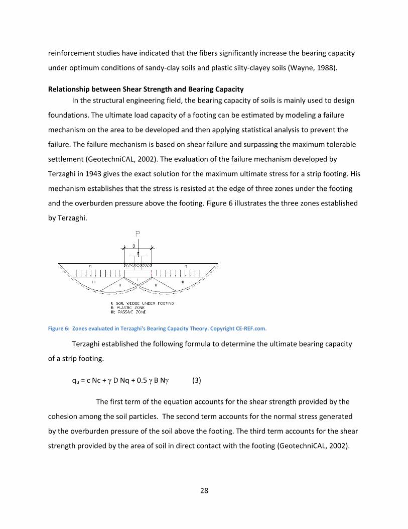
Terzaghi in 1943 gives the exact solution for the maximum ultimate stress for a strip footing. His

mechanism establishes that the stress is resisted at the edge of three zones under the footing

and the overburden pressure above the footing. Figure 6 illustrates the three zones established

by Terzaghi.

Figure 6: Zones evaluated in Terzaghi's Bearing Capacity Theory. Copyright CE-REF.com.

Terzaghi established the following formula to determine the ultimate bearing capacity

of a strip footing.

qu = c Nc + D Nq + 0.5 B N (3)

The first term of the equation accounts for the shear strength provided by the

cohesion among the soil particles. The second term accounts for the normal stress generated

by the overburden pressure of the soil above the footing. The third term accounts for the shear

strength provided by the area of soil in direct contact with the footing (GeotechniCAL, 2002).

29

In conclusion, the bearing capacity of a soil is governed by soil shear strength. A drastic

increment in the bearing capacity of a soil can prove very useful in many aspects of housing

development. Some of these aspects are to be able to build larger structures, reduce the size of

the footings, increase the erosion control and easily stabilize soil for roads.

A body of previous research work has confirmed that the strength and the stiffness of

soils are improved by randomly mixing fiber reinforcement (Babu & Vasudevan, (2008), Hoare,

D.J. (1979), Andersland and Khattac (1979), Freitag (1986), Maher and Gray (1990), Maher and

Ho (1994), Marandi (2008), Michalowski and Zhao (2002), Wang et al. (2006) and Yetimoglu

(2004)). They also report that the increment in shear strength is related to: the fiber

characteristics, mainly the modulus of elasticity of the fiber, the soil characteristics and the

conditions during testing. Therefore, based on the soil type choice, the most popular and

effective fibers used for reinforcement of cohesive soils were established:

Date palm fiber: This study was performed on Iranian soil samples because in 2003, the

Iranian City of Bam reconstructed the city on soil reinforced with date palm fibers. They

selected this fiber because it is a main agricultural crop in Iran. The study found that the

date palm fiber reaches maximum water absorption of 187% after a 24-hours soaking

period. This condition increases the fiber length by 2.51% and the cross sectional area by

11.11%. The maximum tensile strength of a fiber is 63.32 MPa (8991 psi) and has an average

diameter of 0.35 mm (13 * 10-3 in). The study evaluated the effect of the fiber on the shear

strength and the bearing capacity of the silty sandy soil. The shear strength was evaluated

through Unconfined Compression Tests (UCT). Sixteen samples were prepared for this test.

Two of the samples were the control group (non-reinforced soil), fourteen samples were a

combination of 2 different fiber lengths (20 mm & 40 mm) with seven different fiber

contents expressed as percentage by weight (0.25%, 0.5%, 0.75%, 1.00%, 1.50%, 2.00%,

2.50%). The maximum shear strength of the non-reinforced soil samples was 40 kPa. The

maximum shear strength reached by the reinforcement was the one obtained by the 40 mm

2.50% combination, with maximum shear strength of 530 kPa. This displays an increase of

more than 13 times the strength of the non-reinforced soil. As described in the bearing

30

capacity section of this chapter, this study concludes that the insertion of date palm fiber

into the soil can increase the non-reinforced soil bearing capacity up to 26 times (Marandi,

2008).

Polypropylene fibers (Duomix F20): This study was performed on a soil consisting of a sand

fill overlaid by a soft clay sub-grade. The polypropylene fibers were 20 mm long, had a

diameter of 0.05 mm (1.9 * 10 -3 in) and an average tensile strength of 360 MPa (51122 psi).

The study evaluated the effect of the fiber reinforcement on the bearing capacity of the soil

through CBR tests as described in the bearing capacity section of this chapter (Yetimoglu, et

al. 2005).

Coconut fiber (Coir): This study was performed on a poorly graded sand (SP) type of soil

according to USCS. The researchers selected coconut fiber because it has the greatest

tearing strength among all natural fibers and retains this property in wet conditions. The

study focuses on determining the effect of the reinforcement on the shear strength and the

stiffness of the soil using Triaxial tests. Two hundred and fifty two samples were used for

the testing; the samples were a combination of 3 different fiber diameters (0.15 mm, 0.25

mm, 0.35 mm), 4 different fiber lengths ( 10 mm, 15 mm, 25 mm, 35 mm), 3 different

confining pressures (σ3 = 50 kPa, 100 kPa, 150 kPa) and 7 different fiber contents expressed

as percentage by weight (0.00%, 0.25%, 0.50%, 1.00%, 1.25%, 1.50%, 2.00%, 2.50%). The

results indicate that the maximum strength improvement occurs at fiber content between

2.0-2.5%, this is achieved at about 10-18% strain and this was obtained with 15 mm long

fibers for all confining pressures. The study mentions that the specimens beyond a fiber

content of 2.5% were difficult to prepare because the reinforced soil will clump causing

sample breaking without compression. The conclusion indicates that the maximum increase

of strength is 3.5 times that of the non-reinforced soil samples (Babu & Vasudevan, 2008).

The following chapter is the Methodology, which presents the selected fiber and the

critical information obtained from the literature review that was used for the experimental

design.

31

Chapter 3: Methodology

Selection of Fiber and Experimental Design Parameters

After we reviewed the fiber reinforcement papers, we determined the fiber selection

parameters were the following:

It must not be a hazard to its surroundings.

It must be easily obtainable and inexpensive.

Its preparation method should be simple.

It must work with the selected soil.

We evaluated the fibers presented in the Background Chapter according to these

parameters:

Date Fiber: The cost of date reinforcement is very low and affordable by the developing

countries in Asia. However these fibers are not easily attainable in the other continents.

Polypropylene fibers (Duomix F20): These fibers degrade easily under direct soil

exposure and they are not easily available in developing countries.

Recycled carpet waste: A study by Ghiassian, et al (2004) presents that a soil reinforced

with randomly mixed carpet waste increases its shear strength. A negative aspect is that

the waste preparation for its reutilization is extensive, it is not easily attainable in

developing countries and it significantly alters the environment.

Coconut fibers (coir): These fibers are biodegradable and environmentally friendly.

Additionally, coconut trees grow widely in tropical areas around the world such as Asia,

Central and South America and Africa. Palm trees are grown in abundance in Brazil, the

32

Caribbean, Venezuela, Indonesia, Thailand and Kenya among others (Coconut Palm

Tree, 2003)

We determined we would like to use a natural fiber that was environmentally friendly

and easily attainable worldwide, especially in our focus area. Therefore we selected coconut

fiber as the reinforcement material for this study. Also, coconut fiber is significantly stronger

than date palm fiber, even with a 0.10 mm diameter; coconut fiber is far more available than

polypropylene, and more available worldwide than date palm fiber and coconut fiber is cheaper

than polypropylene. Coir is biodegradable and it takes approximately 20 years to decompose

above ground. However, our testing was done in burial conditions; a few experiments

performed by Rao and Balan (2000) suggest that the fiber will last only 2-3 years in this

condition. Studies have also shown that coating the fibers with a protective layer could increase

its durability. The United States Department of Agriculture (USDA) recommends an all natural

coating to be applied to protect buried wood up to 20 years (Gegner, 2002). We researched the

toxicity of all the substances used for this coating. None of them are toxic to the environment

and the health of living organisms. Therefore we decided to use this coating to increase the

durability of the coir fibers. It is beyond the scope of this project to evaluate the real effect of

the coating on the useful life of the fibers. However, we recommend this test to be performed

in future research.

From the results presented in the previous fiber-reinforcement studies, the effectiveness of

fiber reinforcement depends on fiber concentration and length. Therefore, we designed our

laboratory experiments to identify what is the best reinforcement scheme in terms of fiber’s

concentration and length. The fiber lengths range is between 20 mm and 40 mm and fiber

content range expressed in percentage by weight is between 0.00% and 2.50%. The selection

of tests to determine fiber’s parameters pertinent to reinforcement effectiveness is presented

in the following section.

Selection of Testing Sequence and Procedures

To select the tests we established the main evaluation steps that needed to be

accomplished to determine if the application of the coir reinforcement would be beneficial on

33

the focus geotechnical properties of the project: the bearing capacity and the slope stability of

soil. The established steps are:

1. Evaluate the effect of fiber reinforcement on shear strength of the soil; this includes the

identification of the optimum reinforcement condition in terms of fiber length and

concentration.

2. Test the impact of an increase in shear strength on the soil bearing capacity and

compare it to the bearing capacity value predicted by Terzaghi’s Theory.

3. Analyze the benefits of fiber reinforcement on slope stability.

To accomplish step 1, we first selected the necessary tests to obtain the properties of

coir and the tropical soil that we needed to know in order to test the shear strength of the soil.

These properties were: the tensile strength of the fibers, the effect of the coating on the fibers

and the optimum moisture content (OMC) and the dry and optimum unit weight of un-

reinforced and reinforced soil. To obtain the first two properties we selected the Ultimate

Tensile Strength test. The tensile strength of coir needed to be compared to that of soil to

assure it was significantly larger. It was also necessary to evaluate the effect the coating had on

the fibers to assure the coating wasn’t detrimental to the tensile strength of the fiber.

To obtain the OMC and the dry and optimum unit weights of the soil, we selected the

Standard Proctor Compaction Test with a 5-pound hammer (ASTM D698). These parameters

were important because testing at optimum conditions standardizes the sample preparation

and optimizes the strength of the samples.

To evaluate the effect of the fiber reinforcement on the shear strength of the soil, there

were two options available to us: the Triaxial Test and the Unconfined Compression Strength

Test (UCT). We selected the UCT (ASTM D2166) because the sample preparation time for this

test is significantly shorter than the sample preparation time of the Triaxial Test. Even though

the UCT provided less information than the Triaxial Test, the information was still sufficient to

clearly establish the characteristics of the optimum soil fiber reinforcement scheme. Once the

characteristics of the optimum reinforcement were established, we decided to test the

unconfined compressive strength of completely saturated un-reinforced and optimally

reinforced soil. We considered it is necessary to evaluate the effect of the fibers on the soil

34

structural integrity once the cohesion of the soil particles was practically null. This would occur

under extreme wet weather conditions or flooding.

Also, as suggested by the review of the coir reinforcement study and as observed during the

UCT the fiber reinforcement above 1.5% content by weight retains the structural integrity of

the soil sample above excessive strain percentages. Because there is not a clear failure point

anymore, this behavior impedes the ability clearly distinguish the effect of the different fiber

contents on the soil samples. Therefore a second failure parameter had to be taken into

account. In addition to this second parameter, it was deemed necessary to evaluate the effect

of the fiber reinforcement under tensile stresses. The purpose of this evaluation would be to

determine if the change in parameters of the fiber would have a significant impact on the

tensile strength of the fiber. This was evaluated through Indirect Tensile Strength Test (ASTM

D4123).

To accomplish step 2, we needed to evaluate the effect of the fiber reinforcement on the

foundation bearing capacity of the soil. We determined we would design a foundation bearing

capacity testing procedure capable of being performed in the WPI laboratories. We wanted to

determine the effect of the fiber reinforcement on the construction practices of the low income

communities of Rio de Janeiro, Brazil. The traditional dimensions of a single room adobe house

are the presented in Appendix B. We concluded that we wanted to design a foundation bearing

capacity test, where the footing and surrounding soil was a scale model of the in-situ conditions

for a typical single-room house in Rio de Janeiro.

Table 1Error! Reference source not found. summarizes the testing sequence and the

procedures we selected.

Table 1: Testing Procedures

Test Studied Effect ASTM Standard

Ultimate Tensile Strength Maximum tensile strength of coated and non-coated fibers. Similar to D638

Proctor Compaction Optimum moisture content of non-reinforced and reinforced soil. D698

Unconfined Compression Saturated UCT

Improvement in shear strength of soil through fiber reinforcement. Improved soil structural integrity D2166

Indirect Tensile Change in tensile strength of soil D4123

35

through fiber reinforcement.

Bearing Capacity Improvement in bearing capacity of soil through fiber reinforcement.

We designed the procedure.

To accomplish step 3, we determined the impact of the soil reinforcement on slope stability

by modeling the behavior of a shallow layer of reinforced soil on a hillside and comparing it to

the behavior of a non-reinforced soil on a hillside. Due to time constraints we realized that we

only had time to evaluate the effect of the fiber reinforcement on soil at optimum conditions.

Therefore, we decided to model the improvement of slope stability through the soil

reinforcement without a triggering event, such as an intense rainfall that would increase the

level of the water table. The goal of the models was to determine the maximum slope angle a

hillside can have before failure occurs at normal loading conditions which would occur in a fully

developed area. To perform the modeling we selected a program that is used to analyze the

stability of a slope, called STB2006. The program calculates different factors of safety for a

single slope by taking 25 different circular slip surfaces defined by 25 different centers defined

by the user. At the end, it provides the user with the critical factor of safety which is the lowest

ratio found during the analysis. The program uses Bishop’s simplified method, which as

described in the Current Soil Stabilization Technologies Section of the Background Chapter, is

fairly accurate and easy to apply slope stability analysis method. The program applies

Koppejan’s correction when analyzing very deep slip circles and accounts for a strength

reduction for double sliding cases (STB Software User Manual).

The cost efficient and practical implementation characteristics of the soil fiber

reinforcement made this the ideal method to be studied for the improvement of foundation

bearing capacity and shear strength of a typical tropical soil. The world wide availability, high

tensile strength, minimal preparation and low costs of coconut fiber made this the ideal

material to be used for the fiber reinforcement. The following sections present how the

tropical soil was obtained and how the selected tested were performed.

Soil Selection

36

In order to select the soil type that we would emulate, we did in-depth research about the

development practices of the communities in Rio de Janeiro. Figure 7 exemplifies common

housing construction practices in the low income areas of Rio de Janeiro.

We realized most of the houses in these low-income developments are constructed with

adobe. After reviewing a couple of South American Earth Construction Manuals we concluded

one of the biggest concerns is the micro-cracking caused by either excessive amounts of clay or

lack of medium to large aggregates in the mix. However, the nature of adobe does not allow for

grain sizes larger than 5 mm, therefore light flexible aggregates like straw and fibers have a

positive impact in the adobe mix. The straw and the fibers increase the cohesion among the

soil particles increasing the tensile strength without causing micro-cracking (Delgado &

Guerrero, 2005). We hypothesized that if randomly mixed fibers increased the shear strength of

a soil with properties similar to the perfect soil for adobe, the same fibers would have a positive

impact on the tensile strength of adobe blocks.

Figure 7: Typical low income adobe house in Rio de Janeiro. Copyright VIVERCIDADES, 2006)

The circumstances described for low income communities in Rio de Janeiro Brazil, also

occur in poor communities around the world. Therefore adobe construction is very popular

among these communities. More information about locations of these communities worldwide

and practices of adobe construction can be found in Appendix B.

37

The best adobe blocks are produced using a soil mix with the following ranges of

percentages by weight of soil materials (Delgado and Guerrero, 2005):

Table 2: Optimum soil for Adobe composition

Soil Type Percentage by Weight

Clay 8 -25

Silt 10 - 25

Sand 45 -70

Fine Gravel (less than 5 mm Dia) 2 - 5

The soil in Rio de Janeiro that had a particle distribution closest to the range of perfect soils

for adobe was a sandy clay loam. A tropical soil study by Dieckow (2009) performed in Brazil

presented that the sandy clay loam of this area has in average the following percentages of soil

by weight: 18% clay, 22% silt, 55% sand and 4% other components such as organic matter. We

won’t include organic matter into the soil for our study because this would interfere with the

interaction between the fibers and the soil. In addition the Adobe Manuals strongly

recommend not including gravel particles bigger than 5 mm in diameter. Therefore our soil

cannot be identical to the soil described in the Brazil study. Following the Soil Taxonomy

Classification Pyramid present in 8 we determined, the percentages by weight of soil types that

compose a sandy clay loam vary within the ranges presented in Table 3.

Figure 8: Taxonomy Soil Classification Pyramid. Copyright NRCS, 2009.

38

Table 3: Ranges of soil percentages by weight for sandy loam

Soil particle Percentage by weight range

Clay 10 - 35

Silt 0 - 28

Sand 50 - 80

The taxonomy classification system is an agricultural classification system since its

categories account for the type and content of organic matter. Our project focuses on the

behavior of the inorganic matter with the fibers. Therefore we transferred the taxonomy

classification into the geotechnical soil classification system: the Unified Soil Classification

System (USCS). Under this classification a silty clayey soil with these characteristics will fall in

the SM-SC classification of the USCS (Dieckow, 2009). We decided this cohesive soil type would

be ideal for our project. Therefore the fiber to be selected had to mix well with the SM-SC soil

and significantly increase the shear strength of the soil.

Soil Synthesis

As mentioned in the Soil Selection section, the tropical soil we decided to synthesize

was a silty clay sand (SC-SM ) similar to a sandy clay loam found in Rio de Janeiro, Brazil. In

order to synthesize this soil we designed the following particle distribution for our soil. We

obtained a unit weight range of 100 to 130 lbs/ft3 for an SC-SM soil from the Military Science

Soil Classification Manual (FM5-410). The average of the unit weight range is 120 lbs/ft3, which

we used to estimate the total soil weight that we needed to complete each test. Table Error!

Reference source not found.4 summarizes the pounds of soil necessary for each test. We

calculated the weights by multiplying the dry unit weight of the soil by the volume of each test

sample and then we multiplied it again by the number of samples required for each test.

Table 4: Lbs of soil required per set of tests

Test Lbs of soil

Proctor Compaction 13

Unconfined Compression (UCT) 107

Indirect Tensile (ITT) 30

Saturated UCT 17

Bearing Capacity 395

39

Total lbs of soil 562

Once we knew the total weight of soil required, we ordered and sieved the

different soil types. Based on the NRCS Taxonomy Classification table we approximated we

would need 400 lbs of medium grade sand provided by WPI (further referred to as WPI Sand),

75 lbs of beach sand, 100 lbs of clay, 125 lbs of silt and 75 lbs of #8 fine aggregate. The sand

provided by WPI had a particle distribution different from the particle distribution we had

determined we needed for our soil. Therefore we sieved 500 lbs of medium grade sand, and

used only 400 lbs of the particles we needed. The WPI sand had to be sieved using sieves sizes

No. 4, and No 8. We then discarded all of the particles left on sieve No. 4 and used 18.5 percent

by weight of the particles left on sieve No. 8. All other sand particles that passed through the

sieve were used in creating our soil.

An in-depth description of the particle distribution analysis is presented in the Analysis

& Results Chapter. We ordered the clay from Active Mineral International (Acti-Min). A Brazilian

study of soil types in Rio de Janeiro (Vieira & Monteiro, 2007), determined that most of the clay

found in this area is a plastic kaolin type of white color. Acti-Min offered two types of 100%

kaolin clays, one coarser than the other one; therefore we decided to order 50 lbs of each type

and mix them. The first type was the Acti-Min CR which is general filler kaolin with typical

moisture and residue control qualities. The second type was the Acti-Min Cast which is coarse

particle kaolin with excellent drainage qualities. We ordered the silica from Akron, Ohio. We

ordered 200 lbs of Sil-Co-Sil.

Once we obtained all the ingredients, we approximated each of their unit weights. We

accomplished this by measuring 500 ml of each soil type and weighing them. With this unit

weights, we designed the ideal particle distribution for the tropical soil. Table 5 summarizes the

unit weights of the soil types and shows the percentage by weight of each soil type to

synthesize our ideal soil sample.

Table 5: Ideal Soil Particle Content

Soil Type Unit weight (lbs/ft3) Percent Content Weight of soil for 1 ft3 (lbs)

WPI Sand 130 70.00% 91

40

Beach Sand 127 5.00% 6.35

Clay 35 8.00% 2.8

Silt 75 10.00% 7.5

# 8 Fine Aggregate 135 7.00% 9.45

Final unit weight 117.1

The best way to mix the soil was to use WPI’s concrete mixer, which allowed us to mix 1 cubic

foot of soil per batch. As the last column of Table 5 presents, we added those weights of each

soil material to each batch. Each batch was mixed for approximately 7 minutes. We did a total

of 5 tropical soil batches. Then we ran a particle distribution analysis of the finalized soil. Table

6 summarizes the results of the soil types we obtained from the particle distribution analysis.

Table 6: Actual Soil Type Content

Soil Type Unit weight (lbs/ft3)

Percent Content Weight of soil for 1 ft3 (lbs)

WPI Sand 130 67.00% 87.1

Beach Sand 127 6.00% 7.62

Clay 35 9.00% 3.15

Silt 75 10.00% 7.5

# 8 Fine Aggregate 135 8.00% 10.8

Final unit weight 116.17

Figure 9A illustrates the WPI Sand Particle Distribution Analysis. Figure 9B illustrates the

weighing of the soil materials for the soil synthesis process.

Figure 9A: WPI Sand Sieve Analysis. Figure 9B: Weighing of the Soil Materials for Mixing

41

Once we synthesized enough tropical soil to run all tests, we began the testing sequence

by performing the Proctor Compaction Test (PCT).

Fiber Preparation

We obtained the coconut fiber for the tests from a natural textiles company called

Rolanka International Inc. located in Georgia, U.S. We ordered 18 lbs of the coir fiber which

came in a bale size bundle. We measured the diameter of 5 different randomly selected fibers.

The average diameter of a single fiber was 0.35 mm (1.4 x 10-2 in). During the handling of the

fibers we assessed qualitatively that the fibers had minimal moisture content. We noticed that

even though no moisture was detected the fibers had a fairly elastic behavior. The fibers

lengths varied between 18 to 24 inches. Figure 10 illustrates the comparison of the fibers

dimensions with the dimensions of a dime.

Figure 10: Comparison of fiber dimensions with a dime.

As previously described, experiments performed on coir fiber placed underground

suggest that the fibers will degrade in a period of 2 to 3 years. Therefore, we decided to protect

42

the fibers with the all-natural preservation coating recommended by the USDA. The

ingredients we used to coat the fiber were:

1½ cup boiled linseed oil

1 ounce of paraffin (substitute carnauba or wood rosin wax, provided they contain no

prohibited substances)

Enough solvent (distilled pine tar, mineral spirits, paint thinner, turpentine, citrus thinner,

or whatever is approved) at room temperature to make the total volume of the mix one full

gallon.

To make the mix we melted the paraffin over water in a double boiler. Once the

paraffin had melted we poured it into a separate container with the citrus solvent. We added

the linseed oil and continued to stir the mix until it was a homogenous solution. Then we

submerged handfuls of fiber into the mix and let them sit for 7 minutes. Figure 11 illustrates the

consistency of the coating. Once the fibers were coated we let them dry for approximately 48

hours.

Figure 11: Complete mix of coating

Table 7 presents the weight of coated fibers needed for each test. From the total weight

presented in the table, we determined 10 pounds of coated fibers would be sufficient for all

tests. The weight of the coated fibers necessary for each experiment was calculated as 2% of

the total weight of soil required for each individual test. We approximated a 2% content by

weight of fiber for each test because this is the average of the fiber content by weight range

43

obtained from the literature review. The calculation of the required amount of soil for each test

will be explained in the Soil Synthesis section of this chapter.

Table 7: Lbs of Coated Fiber required per set of tests

Test Lbs of Reinforced Soil = volume of mold * Optimum Unit weight (135 lbs/ft^3) Lbs of Coated Fibers

Proctor Compaction 10 0.2

Unconfined Compression (UCT) 108 2.16

Indirect Tensile (ITT) 27 0.54

Saturated UCT 13.5 0.27

Bearing Capacity 295 5.9

Total lbs of coated fibers needed 9.07

As concluded in the Fiber Selection section the lengths of the fibers needed to be within

a range of 20 to 40 mm. We decided to test two different lengths of fibers; one of the lengths

would be within this range (35 mm) and the second one would be outside this range (50 mm) in

case the fibers behave differently than as predicted by the literature review. The bearing

capacity test was based on a scaled down model of the real circumstances. Therefore the fibers

required for this test needed to be a scaled down version of the optimum fiber length.

Figure 12: Fiber cutting process

Figure 12 illustrates the cutting process of the fibers. The instruments used were a

paper cutting board and scissors. This process was very time consuming and required a lot of

44

effort to ensure most of the fibers had the desired lengths. We ran a second control of the

fiber length by sieving the fibers horizontally through a 1 ½” sieve.

Testing

1. Tensile Strength Test of Coconut Fiber

The purpose of this test was to determine the effect of the coating on the fiber’s tensile

strength. We established this by testing the strength of coated and non-coated specimens, and

then we compared the results. If the coating had presented an extremely detrimental effect on

the fibers’ strength, we would not have used the coating for this study. In such a case we would

have tested the effect of non-coated fibers in soil reinforcement, and we would have

recommended that future research should find a protective process that did not have such a

negative impact.

To determine the tensile strength of the fibers we took 10 individual randomly selected

fibers and twisted them together by hand. Then we glued them to plastic squares using Epoxy

glue, the plastic squares had dimensions of 1” x 2”. Figure 13 illustrates this process.

Figure 13: Preparation of coated-fiber samples for Ultimate Tensile Test.

After the glued samples dried for 24 hours, we placed the plastic ends into the Sintech

5/G machine, which held each end with a vise to securely hold the test specimen. We

performed an assessment of the coated and non-coated fibers. We concluded there was not a

45

difference in texture between the two groups. The only way we could differentiate between

them was from the smell coming off the coated fibers. We tested 4 specimens of coated fibers

and 4 specimens of non coated fiber.

2. Proctor Compaction Test

The Proctor Compaction Test (PCT) provided us with the optimum moisture content at

which the maximum unit weight of our soil was achieved. We used a proctor test with the

procedure established by ASTM D698. This procedure uses a 4-inch diameter mold which holds

1/30th cubic foot of soil, and calls for compaction of three separate layers of soil using 25 blows

by a 5.5 lb hammer falling 12 inches, for a compaction effort of 12,400 ft-lbf/ft³. Compaction is

the process of increasing the bulk density of a soil by driving out air. The density obtained

depends on the moisture content of the soil, which we determined by increasing the moisture

content of each test by 4%.

For our proctor test we took moisture contents of 4%, 8%, 12%, 16%, and 20%. We then

made one mold for the five different moisture contents. We did this for both unreinforced

samples and reinforced samples. We initiated each test by weighing out ten pounds of soil, and

then adding the required amount of water to reach the specified moisture content. We

obtained the moisture content with the following equation: 𝑀𝐶% =𝑊𝑤𝑎𝑡𝑒𝑟

𝑊𝑑+𝑊𝑤𝑎𝑡𝑒𝑟. Where MC %

is moisture content, 𝑊𝑤𝑎𝑡𝑒𝑟 is weight of water and 𝑊𝑑 is dry weight of our soil. Once the water

was added to the soil we mixed them together manually by hand, until the soil achieved the

desired moisture content throughout. Figure 14 illustrates one of the mold specimens of the

fiber reinforced PCT.

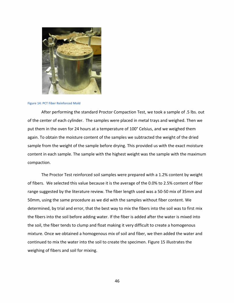
46

Figure 14: PCT Fiber Reinforced Mold

After performing the standard Proctor Compaction Test, we took a sample of .5 lbs. out

of the center of each cylinder. The samples were placed in metal trays and weighed. Then we

put them in the oven for 24 hours at a temperature of 100° Celsius, and we weighed them

again. To obtain the moisture content of the samples we subtracted the weight of the dried

sample from the weight of the sample before drying. This provided us with the exact moisture

content in each sample. The sample with the highest weight was the sample with the maximum

compaction.

The Proctor Test reinforced soil samples were prepared with a 1.2% content by weight

of fibers. We selected this value because it is the average of the 0.0% to 2.5% content of fiber

range suggested by the literature review. The fiber length used was a 50-50 mix of 35mm and

50mm, using the same procedure as we did with the samples without fiber content. We

determined, by trial and error, that the best way to mix the fibers into the soil was to first mix

the fibers into the soil before adding water. If the fiber is added after the water is mixed into

the soil, the fiber tends to clump and float making it very difficult to create a homogenous

mixture. Once we obtained a homogenous mix of soil and fiber, we then added the water and

continued to mix the water into the soil to create the specimen. Figure 15 illustrates the

weighing of fibers and soil for mixing.

47

Figure 15: Adding fibers to the soil.

An important observation we noticed during the preparation of the 20% moisture

content reinforced sample, is that the fibers significantly modify the behavior of the wet soil

from a liquidly-muddy state to a material with structural integrity that can be held. Figure 16

illustrates the consistency of the 20% MC reinforced sample.

Figure 16: 20% MC Reinforced Soil Sample Preparation

3. Shear Strength Test

The shear strength test was done to determine the optimum fiber content percentage

and fiber length for reinforced soil. The Unconfined Compression Test method covers the

determination of the unconfined compressive strength of cohesive soil in the intact, remolded

or reconstituted condition, using strain controlled application of the axial load, according to the

48

ASTM D2166-06 Standard Test Method for Unconfined Compressive Strength of Cohesive Soil.

The fast loading of the soil sample does not allow the water to flow out of the sample;

therefore this test determines the soil’s un-drained shear strength.

This test loads a sample vertically while having no compression laterally until the sample

fails due to shear or compresses too much. To assure the scientific validity of the test, we

deemed sufficient to test a minimum of three specimens per sample group. The test was done

creating the same cylinders that we made in the Proctor Test. The moisture content we used

for the samples was the Optimum Moisture Content (OMC) of 7.5%, which we determined from

the results of the PCT. In total we created 24 cylinders. Table 8 summarizes the samples that

were tested to study a range of values for the fiber lengths and the fiber content percentages.

Table 8: UCT Specimens

To create the cylinders for the UCT, we followed the standard sample preparation

procedures normally used for the PCT. Once the soil was compacted into the molds, we

extruded them from the mold and placed them on a metal tray. This was a standard procedure

we established during the sample preparation to minimize the modification of the samples

compaction. During the compression of the samples, the tray acted as a barrier that collected

the soil to be reused. Figure 17 illustrates how the samples were placed during testing.

# of Cylinders Fiber Length Fiber %

3 35mm 0.8

3 50mm 0.8

3 35mm 1.8

3 50mm 1.8

3 35mm 2.4

3 50mm 2.4

3 50mm 3.2

3 0mm 0

Total Tests=24

49

Figure 17: Placing an UCT sample

We used a loading cell that had a maximum loading capacity of 5,000 lbs. The machine

we used was Sintech 5/ G. This is a highly reliable digital machine that provides its users with

graphical results in addition to the data for direct analysis.

While mixing the soil and fibers together we observed that once the fiber content had

exceed 1.8% it was very difficult to manipulate the soil and obtain a thorough mix. The

procedure for preparing the molds was very time consuming because the fibers would clump

together, and we had to continuously separate the clumps by hand. This problem was noted for

both the 35mm and 50mm fibers lengths. At fiber contents above 1.8%, the soil specimen did

not compact well and the layers would separate easily from one another. During the testing,

we also observed that specimens above 1.8% fiber content never achieved failure. Since the

fibers were so close together they would behave as a mesh that would induce the soil to

recompress. In these cases the maximum loading was achieved. The cylinders without

reinforcement compacted much better than those with fiber reinforcements.

50

Figure 18A: Non-Reinforced Failure Figure 18B: 3.2% Reinforced Failure

Figure 18A illustrates that the samples with no fiber content presented cracks only on

the upper part of the sample at failure. The same behavior was observed for samples with low

fiber (0.8%) content. Meanwhile Figure 18B illustrates that the reinforced samples (1.8% or

more) presented cracks throughout the sample at failure.

As described in the Selection of Testing and Procedure section, we decided to perform

Saturated Unconfined Compression Test to evaluate the effect of reinforcement on completely

saturated soil because there was no existing testing data on the subject. We wanted to

evaluate if the fibers retained the structural integrity of the soil samples as effectively as

before. We followed the same sample preparation procedures as we did for the UCT. We did

three specimens of un-reinforced soil and three specimens of optimum reinforced soil (2.4% 35

mm). Each specimen was soaked in a water-filled container for 72 hrs. Then we took each

specimen out of the water and we put it in a plastic bag. Then we let it sit for 72 hrs because we

wanted the water to distribute evenly within each specimen. Then we ran the compression test

as described in the UCT section.

4. Indirect Tensile Strength Test

As discussed in the Selection of Testing Sequence and Procedures Section of this

Chapter, at fiber contents above 1.8% the soil samples began to recompress after failure has

occurred. The compression behavior of the samples is almost linear throughout the tests; which

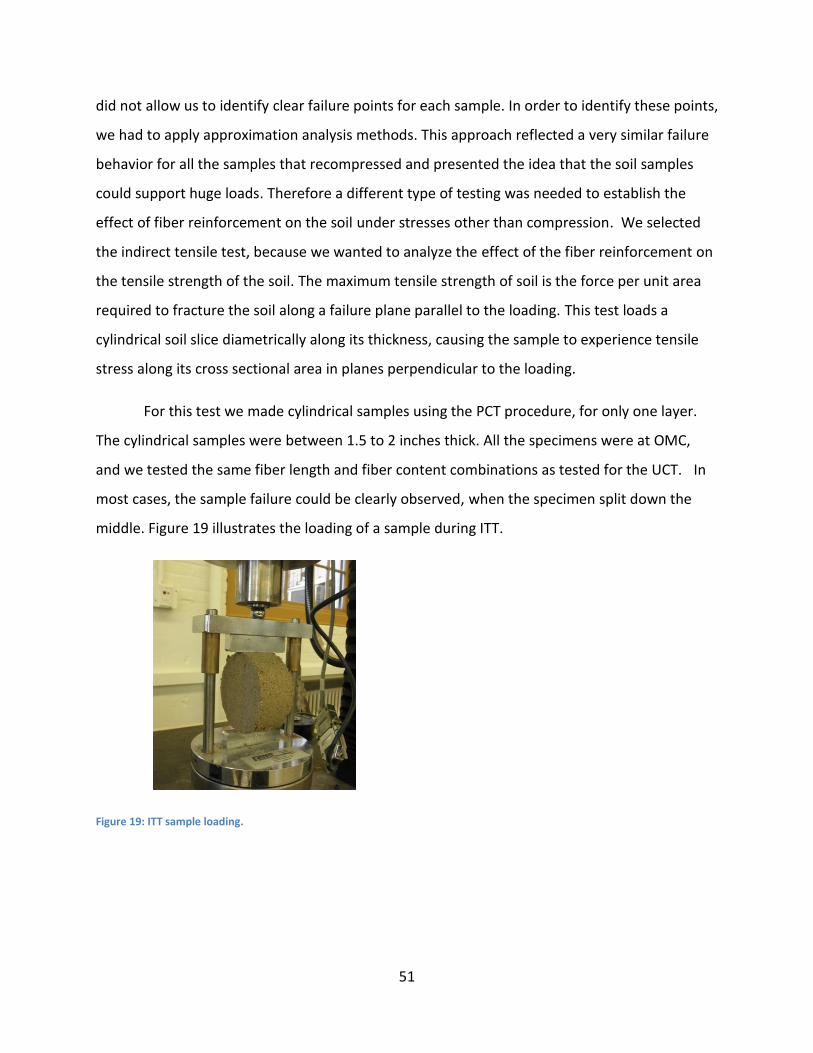
51

did not allow us to identify clear failure points for each sample. In order to identify these points,

we had to apply approximation analysis methods. This approach reflected a very similar failure

behavior for all the samples that recompressed and presented the idea that the soil samples

could support huge loads. Therefore a different type of testing was needed to establish the

effect of fiber reinforcement on the soil under stresses other than compression. We selected

the indirect tensile test, because we wanted to analyze the effect of the fiber reinforcement on

the tensile strength of the soil. The maximum tensile strength of soil is the force per unit area

required to fracture the soil along a failure plane parallel to the loading. This test loads a

cylindrical soil slice diametrically along its thickness, causing the sample to experience tensile

stress along its cross sectional area in planes perpendicular to the loading.

For this test we made cylindrical samples using the PCT procedure, for only one layer.

The cylindrical samples were between 1.5 to 2 inches thick. All the specimens were at OMC,

and we tested the same fiber length and fiber content combinations as tested for the UCT. In

most cases, the sample failure could be clearly observed, when the specimen split down the

middle. Figure 19 illustrates the loading of a sample during ITT.

Figure 19: ITT sample loading.

52

Figure 20A: Non-reinforced ITT Failure Figure 20B: 1.8% ITT Failure Figure 20C: 2.4% ITT Failure

Figures 20A-B-C illustrates the behavior of different reinforced soils under indirect

tension loading. It can be observed that failure occurs in the middle of the cross sectional area

parallel to loading.

5. Bearing Capacity Test

The bearing capacity of a soil is the maximum average contact pressure between a

foundation and a soil before the soil fails due to shear. The bearing capacity test was done to

determine the ultimate bearing stress that our scaled down optimum reinforced soil could

withstand from a scaled down version of a typical low income house footing. The parameters of

the optimum reinforcement were determined on the previously performed tests. We obtained

the ultimate bearing capacity of the un-reinforced and of the optimum reinforced soil, so that

we could compare them and quantify the advantages of reinforcing the soil. These values were

obtained by loading the model footing into a wooden box filled with tropical soil until bearing

capacity failure occurred. We established failure as the point where there would occur a drastic

change in the footing settlement behavior or the footing would settle more than 10% its depth.

We ran four tests, which were a combination of two footings scaled down to ratios of 1:4

and 1:7 with reinforced and un-reinforced soil in optimum conditions. The wooden box was

designed so that it would not exert any pressure on the soil slip surface. We determined the

necessary depth of the box based on soil consolidation settlement theory. One of the

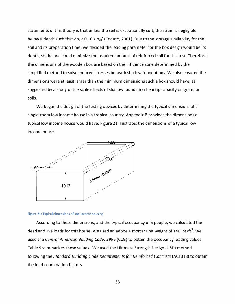
53

statements of this theory is that unless the soil is exceptionally soft, the strain is negligible

below a depth such that ∆σz < 0.10 x σz0’ (Coduto, 2001). Due to the storage availability for the

soil and its preparation time, we decided the leading parameter for the box design would be its

depth, so that we could minimize the required amount of reinforced soil for this test. Therefore

the dimensions of the wooden box are based on the influence zone determined by the

simplified method to solve induced stresses beneath shallow foundations. We also ensured the

dimensions were at least larger than the minimum dimensions such a box should have, as

suggested by a study of the scale effects of shallow foundation bearing capacity on granular

soils.

We began the design of the testing devices by determining the typical dimensions of a

single-room low income house in a tropical country. Appendix B provides the dimensions a

typical low income house would have. Figure 21 illustrates the dimensions of a typical low

income house.

Figure 21: Typical dimensions of low income housing

According to these dimensions, and the typical occupancy of 5 people, we calculated the

dead and live loads for this house. We used an adobe + mortar unit weight of 140 lbs/ft3. We

used the Central American Building Code, 1996 (CCG) to obtain the occupancy loading values.

Table 9 summarizes these values. We used the Ultimate Strength Design (USD) method

following the Standard Building Code Requirements for Reinforced Concrete (ACI 318) to obtain

the load combination factors.

54

Table 9: Loading from Central American Building Code

Live load for housing 40 lbs/ft2

Live load for halls 60 lbs/ft2

Dead load for housing roof 15 lbs/ft2

Table 10 presents the ultimate load calculation procedures. According to the CCG, the

strip footing for our adobe house prototype would have the dimensions presented in Figure 22.

This is a 1 foot long rectangular section of the strip footing for the house. This footing will carry

the equivalent load of 1 ft of U per linear foot. Therefore the design load applied in the footing

equals: P = 137950 / (20‘x2 + 16’x2) = 1916 lbs.

Table 10: Ultimate Load Calculations

Total Live Load = (Assuming 1/3 of the room is used as hall)

20’ x 16’ = 320 ft2 LL = 320x2/3x40 + 320x1/3x60 LL = 14935 lbs

Walls Dead Load = 10’ x 1.5’ x(20’+16’) = 540 ft3 DL = 540 ft3 x 140 lbs / ft3 = 75600 lbs

Roof Dead Load = DL = 320 ft2 x 15 lbs / ft2 = 4800 lbs

Ultimate Load = 1.4 DL + 1.7 LL U = 1.4 (75600 +4800) + 1.7 (14935) U = 137950 lbs

Figure 22: 1 ft long housing strip footing

In order to determine the scale of our footing model, we performed an iterative process

of calculating ∆σz and σz0’. We calculated the applied load value according to the size of the

scaled down footing, and we modified the maximum depth of the influence zone according to

the results. Equation 3 is the approach we used to calculate ∆σz at the maximum depth (zf):

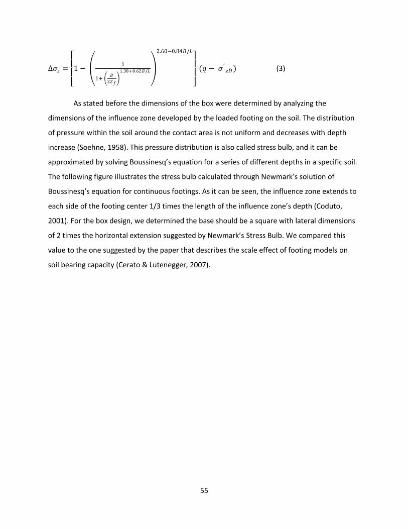
55

∆𝜎𝑧 =

1 − 1

1+ 𝐵

2𝑍𝑓

1.38+0.62𝐵/𝐿

2.60−0.84𝐵/𝐿

(𝑞 − 𝜎 ′ 𝑧𝐷) (3)

As stated before the dimensions of the box were determined by analyzing the

dimensions of the influence zone developed by the loaded footing on the soil. The distribution

of pressure within the soil around the contact area is not uniform and decreases with depth

increase (Soehne, 1958). This pressure distribution is also called stress bulb, and it can be

approximated by solving Boussinesq’s equation for a series of different depths in a specific soil.

The following figure illustrates the stress bulb calculated through Newmark’s solution of

Boussinesq’s equation for continuous footings. As it can be seen, the influence zone extends to

each side of the footing center 1/3 times the length of the influence zone’s depth (Coduto,

2001). For the box design, we determined the base should be a square with lateral dimensions

of 2 times the horizontal extension suggested by Newmark’s Stress Bulb. We compared this

value to the one suggested by the paper that describes the scale effect of footing models on

soil bearing capacity (Cerato & Lutenegger, 2007).

56

Figure F 1: Stress bulb for a continous footing according to Newmark's Solution of Bousinessq's Equations

This paper suggests the horizontal extension of the influence zone is between 2.5 and

12 times the width of the footing (B) according to the soil friction angle, between 28° and 45°

respectively (Cerato & Lutenegger, 2007). The internal friction angle of soft silty clayey sands is

typically between 8° and 20° (Ginzburg, Korchagina, and Shvets, 1995). We realized cohesive

soils transfer stress more effectively than granular soils therefore the relationship between

horizontal extension and friction angle of granular soils cannot be directly applied to this

design. Therefore we based our design around Newmark’s solution, but we made sure the

proposed solution was within the range suggested by Cerato and Lutenegger (2007).

We analyzed different box dimensions by plotting different influence zones according to

the model footing dimensions. We determined the best footing scale and box dimensions to

use were a footing with a scale of 1:7, illustrated in Figure 23 and the box dimensions presented

in Figure 24.

57

Figure 23: Scaled down footing

Figure 24: Bearing Capacity Test Box

Table 11 presents the calculations performed to complete the design of the box.

Table 11: Calculations

𝑞 =𝑃 + 𝑊𝑓

𝐴− 𝑢𝐷 =

1916

scale factor lbs + (487 pcf ∗(1.15”∗1.7”∗(2.6”+5”))/123)

2.6*1.7/144− 0 =

9053.81 psf = 62.87 psi

∆𝜎𝑧 =

1 −

1

1 + 𝐵

2𝑍𝑓

1.38+0.62𝐵/𝐿

2.60−0.84𝐵/𝐿

(𝑞 − 𝜎 ′ 𝑧𝐷)

= 0.1508 psi

10% 𝜎′𝑧𝑑 = 𝑍𝑓 ∗ 𝛾 ∗ 10%

144

= 1.65 ft * 138 lbs/ft3 * 0.1 / 144 = 0.1582

psi

It can be seen that Δσz < 10% σ’zd therefore, the box design won’t interfere with the

influence zone of the footing on the soil. In order to determine the least maximum loading that

should be achieved; we predicted the soil bearing capacity using Vesic’s Bearing Capacity

Theory. This theory follows the same concept as Terzaghi’s Theory, described in the Bearing

Capacity Section of the Background Chapter. The main difference is the way the shape factors

are calculated. Vesic’s factors depend on φ' and adjust more accurately to rectangular footing

shapes than Terzaghi’s do (Vesic, 1973).

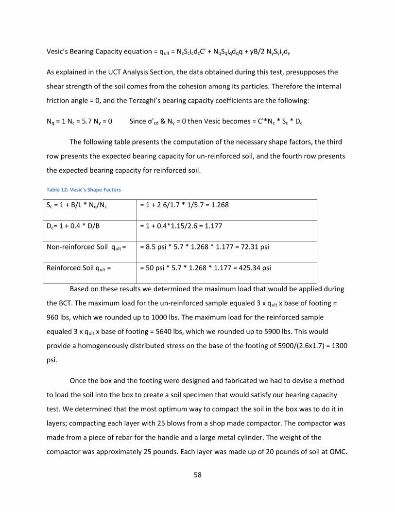
58

Vesic’s Bearing Capacity equation = qult = NcScicdcC’ + NqSqiqdqq + γB/2 NγSγiγdγ

As explained in the UCT Analysis Section, the data obtained during this test, presupposes the

shear strength of the soil comes from the cohesion among its particles. Therefore the internal

friction angle = 0, and the Terzaghi’s bearing capacity coefficients are the following:

Nq = 1 Nc = 5.7 Nγ = 0 Since σ'zd & Nγ = 0 then Vesic becomes = C'*Nc * Sc * Dc

The following table presents the computation of the necessary shape factors, the third

row presents the expected bearing capacity for un-reinforced soil, and the fourth row presents

the expected bearing capacity for reinforced soil.

Table 12: Vesic's Shape Factors

Sc = 1 + B/L * Nq/Nc = 1 + 2.6/1.7 * 1/5.7 = 1.268

Dc= 1 + 0.4 * D/B = 1 + 0.4*1.15/2.6 = 1.177

Non-reinforced Soil qult = = 8.5 psi * 5.7 * 1.268 * 1.177 = 72.31 psi

Reinforced Soil qult = = 50 psi * 5.7 * 1.268 * 1.177 = 425.34 psi

Based on these results we determined the maximum load that would be applied during

the BCT. The maximum load for the un-reinforced sample equaled 3 x qult x base of footing =

960 lbs, which we rounded up to 1000 lbs. The maximum load for the reinforced sample

equaled 3 x qult x base of footing = 5640 lbs, which we rounded up to 5900 lbs. This would

provide a homogeneously distributed stress on the base of the footing of 5900/(2.6x1.7) = 1300

psi.

Once the box and the footing were designed and fabricated we had to devise a method

to load the soil into the box to create a soil specimen that would satisfy our bearing capacity

test. We determined that the most optimum way to compact the soil in the box was to do it in

layers; compacting each layer with 25 blows from a shop made compactor. The compactor was

made from a piece of rebar for the handle and a large metal cylinder. The weight of the

compactor was approximately 25 pounds. Each layer was made up of 20 pounds of soil at OMC.

59

Figure 25A: Bearing Capacity Test Figure 25B: Failed reinforced soil

Figure 25A illustrates the Bearing Capacity Test configuration. Figure 25B illustrates how

the model footing settled more than 10% of its depth. This test was performed with two

different scaled down footings. The first footing was scaled down 7 times its real size. The

results obtained during this test did not present a clear change in settlement behavior but did

present a clear improvement in bearing capacity when testing the reinforced soil. The second

footing was scaled down 4 times its real size. The soil behaved very similar to the soil in the 1:7

scale tests. We considered the possibility that the box was interfering with the compression

influence zone of the footing, and was now allowing the soil to slide along the just developed

slip surface.

The results of the six tests described above can be found in the following chapter. The

next section describes how we evaluated the impact of the shear strength improvement in the

slope stability through the modeling of implementation scenarios.

Modeling of Slope Stability with Soil Fiber Reinforcement

The goal of developing different slope models with the uppermost 3 ft-deep layer of

reinforced soil and determine their factors of safety, was to compare the advantages of using

soil reinforcement on the hillside versus not using reinforcement at all. In order to strictly

60

analyze the effect of the reinforcement in slopes, we kept all the variables unchanged except

for the slope angle, these variables were: dry unit weight of reinforced and non-reinforced soil,

saturated unit weight of reinforced and non-reinforced soil, moisture content and water table

elevation. We analyzed slopes between 27% and 100% steep (between 15° and 45°). We

performed the analysis with the help of a software package named STB. This software

computes the factor of safety of a slope through the simplified Bishop’s method. The models

predicted significant improvement in the slope stability through the fiber reinforcement, for all

the analyzed slopes.

We began the development of the models by establishing the configuration of the

houses on the hillside. We imagined the community development would occur in terraces,

where each terrace would hold 20 ft long houses spaced 10 ft in between. The terraces should

be cut every 25 feet in elevation and not exceed a maximum occupancy of 5 people per house.

Based on the shape of the slip surface used to design the box for the bearing capacity test, we

decided to locate the central axes of the beginning of the strip footing 3xB ft away from the

beginning of the slope, in our case = 4.5 ft. The following figure illustrates the proposed

configuration.

Figure 26: Proposed configuration for development.

61

As mentioned in Appendix B, most developing nations are located in areas of warm to

hot weather with no snow nor freezing temperatures. Therefore the housing building codes of

such countries do not have to account for the minimal depth of footing necessary to prevent

freezing. The recommended maximum depth for shallow strip footing for housing is 2 ft

(CCCA).The low income house model we used is very simple and light; therefore we designed its

footing depth to be 18” or 1.5 ft. Since we wanted the footings to distribute most of the load

across the reinforced soil, we decided to use a 3 ft deep reinforced layer. In this manner the

footing of the model had 1.5 ft of reinforced soil underneath it to distribute the load and

enough soil in the horizontal direction to prevent displacement.

The STB software allows its user to create 2 dimensional areas by determining nodes

and joining lines. Each enclosed area is treated as a soil material, and the program allows the

user to input the following properties of the soil: Dry unit weight (Wd), saturated unit weight

(Ws), coefficient of neutral horizontal stress (Ko), cohesion (c), phi in degrees (angle of internal

friction), groundwater condition (P/F) and thickness of capillary zone (does not apply to our

model). Our model represents two terraces on a hillside and evaluates the stability at the

bottom of one terrace when the terrace above is fully developed according to the plan

described above. The model is composed of 3 different types of soil and the pre-establishment

that the groundwater level = 0 ft. Our first layer of soil (1) represents the un-reinforced soil

(silty clayey sand) at optimum conditions. The second layer of soil (2) represents the uppermost

3 ft of soil. Through the evaluation of the reinforcement effect, this layer obtains the properties

of un-reinforced and reinforced soil. The third layer of soil (3) represents a typical house

according to the dimensions described in the bearing capacity test section. To represent a

typical house, we calculated the house maximum design loading according to LRDF and we

divided it through the volume of the house in order to determine its unit weight. The other

properties for soil 3 were obtained by imagining what properties would prevent failure to occur

in a slip surface through the house. We decided to input a cohesion value significantly larger

than the one for soil 1 and 2, so failure would never occur here before. The following image

presents the input values for soils 1 through 3.

62

Figure 27: STB Software Input Values

Once the model had been created we calculated the factor of safety of the bottom slope

using Bishop’s method through STB. When the safety factor of the slope is less than 1 then the

slope is considered to be unstable. The model was presented in normal conditions, optimum

moisture content and optimum compaction level. The following images illustrates the models

developed for some slope angles and their corresponding failure slip surface for the reinforced

condition.

Figure 28: 37% or 20 degree- slope

Figure 29: 47% or 25 degree-slope

Figure 30: 70% or 35 degree-slope

Figure 31: 84% or 40 degree-slope

The following chapter presents the analysis process for the modeling and the

conclusions we obtained from it.

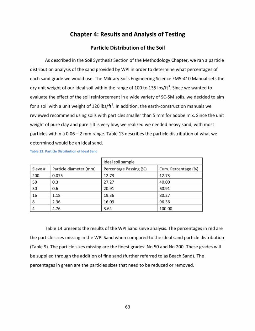
63

Chapter 4: Results and Analysis of Testing

Particle Distribution of the Soil

As described in the Soil Synthesis Section of the Methodology Chapter, we ran a particle

distribution analysis of the sand provided by WPI in order to determine what percentages of

each sand grade we would use. The Military Soils Engineering Science FM5-410 Manual sets the

dry unit weight of our ideal soil within the range of 100 to 135 lbs/ft3. Since we wanted to

evaluate the effect of the soil reinforcement in a wide variety of SC-SM soils, we decided to aim

for a soil with a unit weight of 120 lbs/ft3. In addition, the earth-construction manuals we

reviewed recommend using soils with particles smaller than 5 mm for adobe mix. Since the unit

weight of pure clay and pure silt is very low, we realized we needed heavy sand, with most

particles within a 0.06 – 2 mm range. Table 13 describes the particle distribution of what we

determined would be an ideal sand.

Table 13: Particle Distribution of Ideal Sand

Ideal soil sample

Sieve # Particle diameter (mm) Percentage Passing (%) Cum. Percentage (%)

200 0.075 12.73 12.73

50 0.3 27.27 40.00

30 0.6 20.91 60.91

16 1.18 19.36 80.27

8 2.36 16.09 96.36

4 4.76 3.64 100.00

Table 14 presents the results of the WPI Sand sieve analysis. The percentages in red are

the particle sizes missing in the WPI Sand when compared to the ideal sand particle distribution

(Table 9). The particle sizes missing are the finest grades: No.50 and No.200. These grades will

be supplied through the addition of fine sand (further referred to as Beach Sand). The

percentages in green are the particles sizes that need to be reduced or removed.

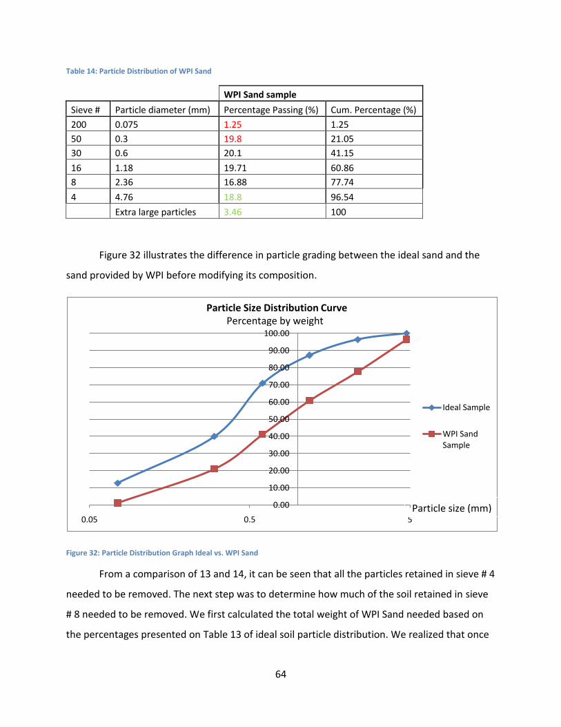
64

Table 14: Particle Distribution of WPI Sand

WPI Sand sample

Sieve # Particle diameter (mm) Percentage Passing (%) Cum. Percentage (%)

200 0.075 1.25 1.25

50 0.3 19.8 21.05

30 0.6 20.1 41.15

16 1.18 19.71 60.86

8 2.36 16.88 77.74

4 4.76 18.8 96.54

Extra large particles 3.46 100

Figure 32 illustrates the difference in particle grading between the ideal sand and the

sand provided by WPI before modifying its composition.

Figure 32: Particle Distribution Graph Ideal vs. WPI Sand

From a comparison of 13 and 14, it can be seen that all the particles retained in sieve # 4

needed to be removed. The next step was to determine how much of the soil retained in sieve

# 8 needed to be removed. We first calculated the total weight of WPI Sand needed based on

the percentages presented on Table 13 of ideal soil particle distribution. We realized that once

0.00

10.00

20.00

30.00

40.00

50.00

60.00

70.00

80.00

90.00

100.00

0.05 0.5 5

Ideal Sample

WPI Sand Sample

Particle Size Distribution Curve

Particle size (mm)

Percentage by weight

65

we compacted the soil, it would increase its unit weight; therefore we would need more soil.

We decided to synthesize 650 lbs of soil.

Total WPI Sand needed: 650 ∗ 70% = 455 lbs

Then, we subtracted the percentage passing through #4 in Table 14 from the percentage

passing through #4 of Table 10 and we multiplied it by the total weight of WPI Sand needed.

455 lbs * (18.8 – 3.46) % = 69.8 = 70 lbs.

Once we had finished obtaining the grades we wanted for the WPI Sand, we synthesized

all the soil. Then we ran a particle distribution analysis of the final soil and we compared it to

the distribution of the ideal soil we had designed. Figure 33illustrates how similar the soil

synthesized compares to the soil we were aiming to obtain. The final unit weight of our soil was

121 lbs/ ft3. According to Table 5 in the Methodology Chapter, our final unit weight should have

been 116.2 lbs/ ft3. We believe the difference in final unit weight can be attributed to loss of

light weight soil materials during the mixing process and to inaccurate measuring procedures of

the individual unit weights.

Figure 33: Tropical Soil Particle Distribution

0.00%

10.00%

20.00%

30.00%

40.00%

50.00%

60.00%

70.00%

80.00%

90.00%

100.00%

0.01 0.1 1 10Particle Size (mm)

Tropical Soil Particle Distribution

Ideal Soil

Final Soil

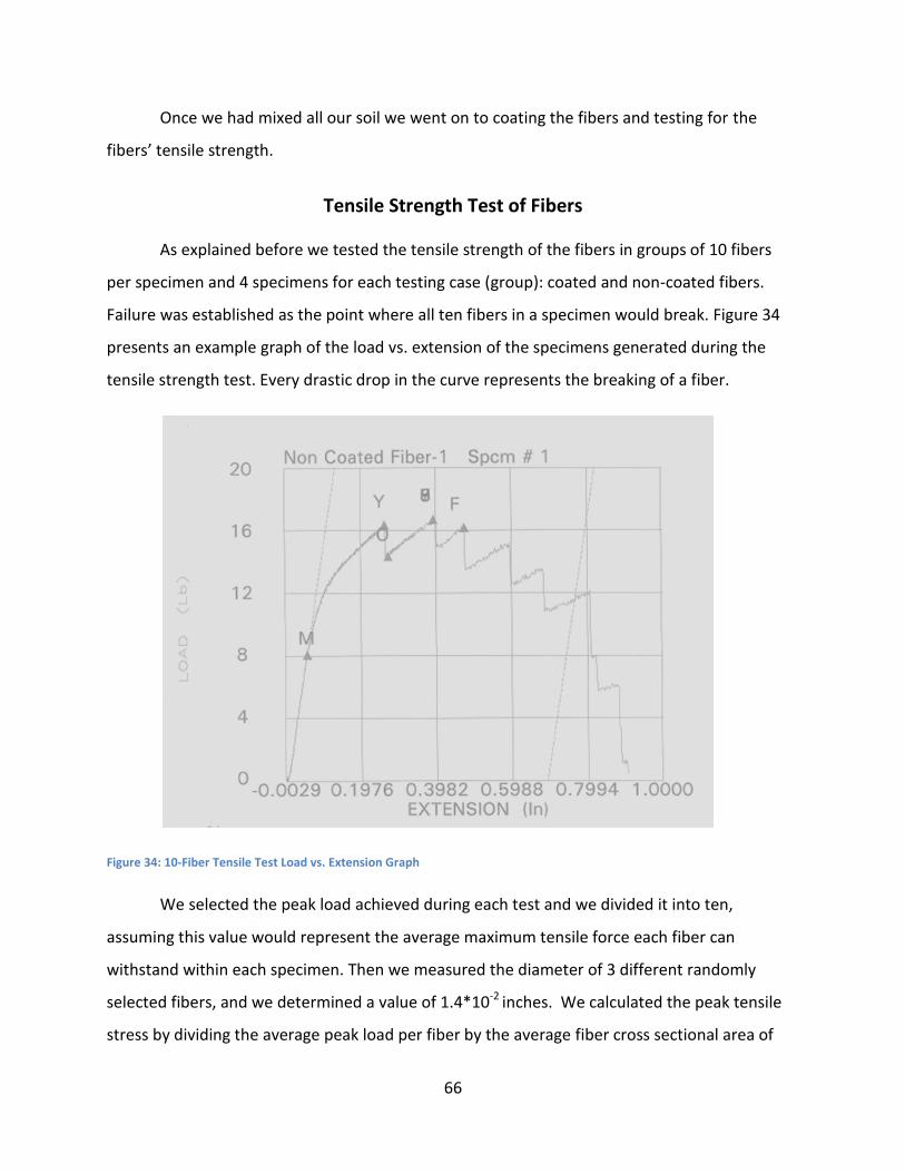
66

Once we had mixed all our soil we went on to coating the fibers and testing for the

fibers’ tensile strength.

Tensile Strength Test of Fibers

As explained before we tested the tensile strength of the fibers in groups of 10 fibers

per specimen and 4 specimens for each testing case (group): coated and non-coated fibers.

Failure was established as the point where all ten fibers in a specimen would break. Figure 34

presents an example graph of the load vs. extension of the specimens generated during the

tensile strength test. Every drastic drop in the curve represents the breaking of a fiber.

Figure 34: 10-Fiber Tensile Test Load vs. Extension Graph

We selected the peak load achieved during each test and we divided it into ten,

assuming this value would represent the average maximum tensile force each fiber can

withstand within each specimen. Then we measured the diameter of 3 different randomly

selected fibers, and we determined a value of 1.4*10-2 inches. We calculated the peak tensile

stress by dividing the average peak load per fiber by the average fiber cross sectional area of

67

15.5*10-5 square inches. Table 15 compares the compares the peak tensile stresses of the

coated fibers vs. the non-coated fibers.

Table 15: Fiber Ultimate Tensile Strength Test Results

Average Tensile Stress per Fiber per Specimen

Specimen # Coated Fibers (PSI) Non-Coated Fibers (PSI)

1 11368.21 10913.48

2 11108.37 10913.48

3 9354.41 12862.32

4 7860.31 10004.02

Average per group 9922.82 11173.33

Percentage Decrease in Tensile Strength (1-Avg C / Avg Non-C) 11.19%

The random selection of the fibers and the heterogeneous nature of this material

allowed for a high variation of fiber diameter and brittleness among the fibers. The standard

deviation of the average maximum tensile stress per specimen among the Coated Fibers group

equals 1640 psi, among the Non-Coated Fibers group equals 1204 psi, and the standard

deviation between the two groups is 1490 psi. Since the variation among groups is higher than

the variation between groups, the test is not scientifically valid. This means that the test is not

100 percent certain that the coating will have a negative effect on the tensile strength of the

fibers. If the effect of the coating needs to be established, this test would have to be run using

standard procedures to control the different possible variables. Some of these are the fibers’

diameters and the uncertainty introduced by the twisting procedure. Another option would be

to design a new test that can measure the pullout strength of the fibers in the reinforced soil.

As it was described in the Fiber Selection Section of the Background Chapter, the

protective coating increases the life of wood under burial conditions up to 20 years. Since the

cross sectional area of our fibers is significantly smaller than that of wood and the constitution

of the fibers is very different than that of wood, we estimate the coating protection method will

add between 8 to 12 years of service life to the fibers on burial conditions. Therefore we

believe the benefits of coating the fiber outdo the benefits of leaving the fiber uncoated. As

explained in the methodology we coated a total of 10 lbs of fiber.

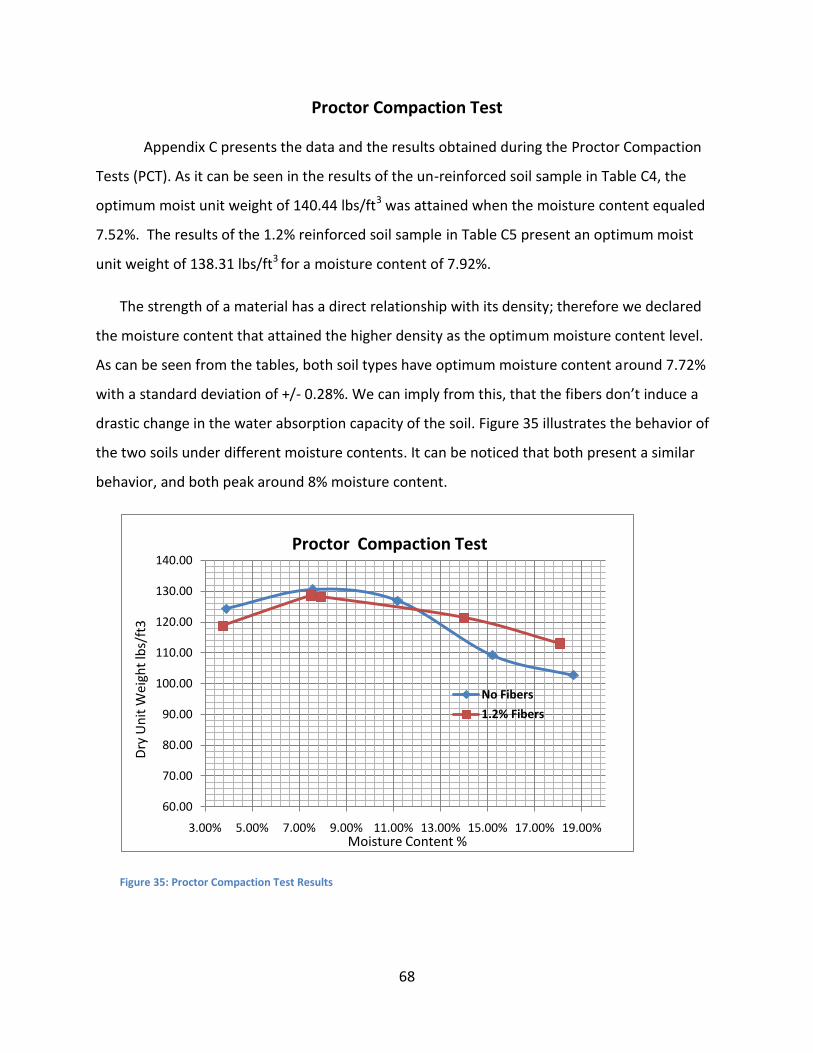
68

Proctor Compaction Test

Appendix C presents the data and the results obtained during the Proctor Compaction

Tests (PCT). As it can be seen in the results of the un-reinforced soil sample in Table C4, the

optimum moist unit weight of 140.44 lbs/ft3 was attained when the moisture content equaled

7.52%. The results of the 1.2% reinforced soil sample in Table C5 present an optimum moist

unit weight of 138.31 lbs/ft3 for a moisture content of 7.92%.

The strength of a material has a direct relationship with its density; therefore we declared

the moisture content that attained the higher density as the optimum moisture content level.

As can be seen from the tables, both soil types have optimum moisture content around 7.72%

with a standard deviation of +/- 0.28%. We can imply from this, that the fibers don’t induce a

drastic change in the water absorption capacity of the soil. Figure 35 illustrates the behavior of

the two soils under different moisture contents. It can be noticed that both present a similar

behavior, and both peak around 8% moisture content.

Figure 35: Proctor Compaction Test Results

60.00

70.00

80.00

90.00

100.00

110.00

120.00

130.00

140.00

3.00% 5.00% 7.00% 9.00% 11.00% 13.00% 15.00% 17.00% 19.00%

No Fibers

1.2% Fibers

Dry

Un

it W

eigh

t lb

s/ft

3

Proctor Compaction Test

Moisture Content %

69

The PCT also provided us with the optimum compacted unit weight for the reinforced soil

(138 lbs/ft3) and the non-reinforced soil (140 lbs/ft3). We designed the implementation of the

next tests around these weights. All the tests for this study must be carried out under optimum

conditions for both soil types because we are aiming to compare the maximum advantages of

reinforcing a soil with natural fibers.

Unconfined Compression Test

The UCT is a strain controlled test; therefore a constant strain rate is applied to the

sample throughout the test. The failure point of the soil sample is determined when the

maximum loading is reached. The fast speed of the loading rate during the test does not give

enough time for the water in the sample to dissipate; therefore the test provides the un-

drained shear strength of the sample. Once the bearing capacity of a soil has been determined,

these results can be used to analyze the factor of safety of the soil under a known sudden

loading.

The data supplied by the unconfined compression test and the stress-strain curves for

each specimen can be found in Appendix D. The test procedure supplied a data table with the

following fields: the applied load, the extension or position of the loader and the elapsed time.

For the purpose of this project we didn’t run a soil time behavioral analysis, therefore the last

field proved unnecessary. We calculated the accumulated length compressed during each

loading increment by subtracting the original position of the loader from the position of the

loader at an x loading. Then we divided the accumulated compressed length by the cylinder

original height of 4.6”. Table 16 exemplifies the described procedure.

Table 16: UCT Data Sample Calculation

Column A B C

Row # Extension (in) ∆H (in) = A2-$A$1 Axial Strain є = B1/4.6”

1 -0.060468 0 0.00%

2 -0.058468 0.002 0.04%

The unconfined compression test cannot provide the measurement of the samples cross

section deformation. However, we wanted to reflect the stress strength capabilities of the soils

70

as accurate as possible, therefore we chose to calculate the stress using the actual area of the

specimen under loading. We decided to modify the cross sectional area of each sample

following a mass conservation model. Our assumption implies that there is not a loss of soil

mass before reaching failure. We also assume that our soil behaves as an ideal fluid therefore it

moves homogeneously through the soil sample and it is incompressible. Therefore:

If the original volume of the soil equals 𝜋 ∙ 𝑟12 ∙ 𝑕1

And the height of the cylinder under loading 2 (h2) equals 𝑕1 ∙ (1 − 𝜖)

Then since the soil density doesn’t change, the conservation of mass assumption implies

that volume at loading 1 has to be identical to volume at loading 2.

Therefore: 𝜋 ∙ 𝑟12 ∙ 𝑕1 = 𝜋 ∙ 𝑟2

2 ∙ 𝑕2 = 𝜋 ∙ 𝑟22 ∙ (𝑕1 ∙ 1 − 𝜖 )

From which can be concluded that area at loading 2 (𝜋 ∙ 𝑟22) = area at loading 1 (𝜋 ∙

𝑟12)/ 1 − 𝜖 .

With this model, we approximated the cross sectional area of the cylinder at the

different loadings in order to calculate the applied compression stress. The following table

exemplifies the corrected area calculation and the applied compression stress calculation.

Table 17: UCT Data Sample Calculation

Column C D E F

Row # Axial Strain є Corrected Area, Ac =$D$1/(1-C1) Load (Lbs) Stress (psi) = E1/D1

1 0.00% 12.56637 1.538653 0.12244212

2 0.04% 12.57139856 2.564421 0.20398852

We calculated the strain and the applied compressive stress for every loading

increment, in every specimen, in every group. Then we identified the peak stress that each

sample could withstand before shear failure. In the case of the samples with 3.2% fiber content,

the layers of compacted soil in each specimen did not bind to one another causing cracks across

the cross sectional area at the binding point. This occurred because the fiber content was too

high; therefore it didn’t allow the soil particles to come sufficiently close to be cohesive with

each other. We believe these cracks did not have a significant impact on the shear failure point

71

of the test because they were perpendicular to the loading direction. No other types of failure

were observed, however shear failure could not always be visually identified. This was the case

for samples with fiber content above 1.8%, where the samples would begin to recompress

before shear cracks could be observed. Figure 36 illustrates the manner in which failure

occurred for each sample type.

Figure 36: A: Non-reinforced B: 0.8% C: 1.8% D: 2.4% E: 3.2% F: Clumping behavior of soil layers with 3.2% fiber content.

As it can be seen, the unreinforced sample opens on the upper end while failing. Large

parts of the sample spall, quickly and significantly decreasing the sample strength. The sample

with 0.8% content opens at the bottom while failing. It can be induced that the fibers are

beginning to redistribute the stresses through the samples. The new location of the cracks

diminishes the spalling. As it can be seen, the samples with content 1.8% to 3.2% seem to be

increasingly retained with a “fiber mesh”. The “mesh” on the 1.8% sample allows for significant

more spalling than the “mesh” on the 3.2% sample. This can be corroborated by comparing the

A

B

C

D

E

E

F

72

amount of spalling and the height in each sample. The samples with the higher fiber content

can sustain more vertical deformation before breaking.

The following figure illustrates the behavior of a non-reinforced soil sample under

unconfined compression stress:

Figure 37: Non-Fiber UCT Specimen 1

While running the tests, we realized that the specimens presented a clear peak stress

before failure only when they were unreinforced or with a fiber reinforcement percentage by

weight of 0.8% or less. Once we incremented the reinforcement to 1.8% by weight, the fibers

would help the soil to remain structurally sound, causing it to compress at even slower rates

than for the unreinforced soil. Due to the load-strain rates the testing machine could not

recognize failure and the stress-strain curve did not produce a clear failure point. The soil re-

compressive behavior allowed the specimens to be loaded past 5000 lbs, the maximum load

available for this test.

In order to determine the failure point of these cases we established two failure

boundaries, from which the lower of the two would represent the failure point. The first

boundary is the point where the stress-strain curve begins to behave linearly. This occurs

because the soil has stopped behaving as a composite soil and instead it has started to behave

0

5

10

15

20

25

30

35

40

45

50

0.00% 5.00% 10.00% 15.00% 20.00% 25.00% 30.00% 35.00%

Non-Fiber UCT Stress vs Strain Curve

Tru

e S

tres

s (

PSI

)

Strain %

73

as a spring. The fibers sustain the remaining soil, preventing loss of soil particles as a single

elastic material. Figure 38 illustrates this behavior by comparing the reinforced soil to a spring.

Figure 38: Representation of soil re-compressive behavior through a spring

Since this new configuration compresses very little every load increment, the machine

can keep on loading at a regular pace until it reaches the maximum load. The following graph

illustrates this approximation procedure for a specimen with 1.8% and 50 mm long fiber

content. Figure 39 illustrates that we performed the approximation procedure on a True Stress

vs Strain curve instead of an Engineering Stress (no change in cross sectional area) vs Strain

Curve (Figure 40). The advantage of using True Stress vs using Engineering Stress when

evaluating the effect of the reinforcement on the soil is that True Stress does not inflate the

final strength values. However, some materials reach a point where the compressive load

remains identical but the cross sectional area of the sample continues to decrease. This causes

the compressive strength of the sample to increase disproportionately, even when the peak

load has been achieved. In these cases it is better to use the Engineering Stress to determine

the sample compressive strength. When Figure 39 and Figure 40 are compared, it can be

noticed that both graphs behave similarly about the point of maximum stress. Therefore, in

this case it is better to analyze the strength of the samples based on True Stress.

74

Figure 39: 1.8% 50 mm UCT True Stress-Strain Curve, Specimen # 2

Figure 40: 1.8% 50 mm UCT Eng. Stress-Strain Curve, Spec. # 2

The linear approximation procedure was the following:

y = 246.8962x + 67.4990R² = 0.9977

0

20

40

60

80

100

120

140

0.00% 5.00% 10.00% 15.00% 20.00% 25.00%

Strain %

Tru

e S

tres

s

(

PSI

)1.8% 50 mm UCT True Stress vs Strain Curve

0

20

40

60

80

100

120

140

160

180

200

0.00% 5.00% 10.00% 15.00% 20.00% 25.00%

1.8% 50 mm UCT Eng. Stress vs Strain Curve

Engi

nee

rin

gSt

ress

( P

SI)

Strain %

75

1) Approximated a point in the graph.

2) Added a trend line to the point values that we believed were part of the linear behavior.

3) Calculated the square of the correlation coefficient for the trend line (R2 ).

4) Select a new set of points and repeated steps 1 and 2.

5) Compared the R2 and selected the set of points with the highest R2.

6) We compared a minimum of 3 different data sets.

The second boundary we established was that the strain caused by the peak stress could

not surpass the allowable strain-stress criteria, which we established would be 18% strain for

this project. This is based on the coir fiber soil reinforcement study performed by Babu and

Vasudevan (2008), mentioned in the Fiber Selection Section of Background Chapter. One of the

main observations of this study is that the maximum strength improvement occurs between a

strain percentage of 10 and 18.

Based on these two boundaries, Table 18 summarizes the stress at failure determined for

each specimen.

Table 18: Peak Stress Summary Table

Peak True Stress in PSI

Spec # 0.00% 0.8% 35 mm 0.8% 50 mm 1.8% 35 mm 1.8% 50 mm 2.4% 35 mm 2.4% 50 mm 3.2% 50 mm

1 18.08 45.72 49.63 64.87 44.72 107.61 138.63 47.88

2 16.7 49.34 50.6 93.66 100.54 86.09 113.64 44.55

3 18.33 55.09 56.06 113.76 75 114.78 48.3 28.94

Once we had determined the failure points of all the specimens we decided to establish the

scientific validity of the tests. In order to establish this, we ran the analysis of variance (ANOVA)

for three different comparisons summarized in Table 19. The assessment consisted of

evaluating the variance within the groups selected for each comparison to the variance

between these same groups. The groups to be evaluated in each comparison differ from each

other by focusing on the strength behavior of the samples with respect to different fiber

parameters. Therefore the first evaluation compares the behavior presented by the un-

reinforced soil to the one caused by different combinations of the fiber length and

concentration parameters. This first comparison needed to be valid to prove the reinforcement

76

introduced a significant improvement in shear strength. Once this was established, the second

evaluation compares the behavior caused by the fiber length and the third evaluation compares

the behavior caused by the fiber concentration. The evaluations were performed in this order

because we considered the first necessary step was to determine if the reinforcement of the

soil with the fibers provided a scientifically valid improvement in the shear strength of the soil

and the effect was significantly different between different combinations; and the second

necessary step was to determine which of the two varied fiber parameters was the leading one:

length or concentration. As our results show, none of them caused a significant effect; there is

an interaction between these two parameters that this test could not determine. However, we

could conclude that the fibers dramatically improve the soil shear strength and there is an

optimum combination of these two parameters.

Table 19: Table summarizing ANOVA Comparisons

Comparison # Groups to be evaluated

1 Control, Specimens reinforced with 0.8% & 35 mm fibers, 0.8% & 50 mm fibers, 1.8% & 35 mm fibers, 1.8% & 50 mm fibers, 2.4% &35 mm fibers, 2.4% & 50 mm fibers, 3.2% & 50 mm.

2 Control, Specimens reinforced with 35 mm long fibers, Specimens reinforced with 50 mm long fibers.

3 Control, Specimens reinforced with 0.8% fibers by weight, 1.8% fibers by weight, 2.4% fibers by weight and 3.2% fibers by weight

The ANOVA test method is appropriate to determine if the difference in the effect of the

reinforcements is significant because the process allows for the comparison of the means of

three or more groups. The test is based on the following two assumptions:

- It is assumed there is zero% error in the measurements.

- The test data follows a normal distribution.

We selected a one way ANOVA test because we wanted to compare just one characteristic

at a time. The test consists of determining whether a hypothesis called the null hypothesis can

be accepted within a pre-established probability called the alpha value. The null hypothesis

states that the variance within the specimens of each group is identical to the variance between

groups. This is evaluated through the F ratio which equals the variance within groups divided by

the variance between groups. Therefore if the null hypothesis is true the F ratio equals 1. If the

77

probability of the F ratio to being 1 is less than the pre-established alpha value then the null

hypothesis is proven wrong, and it can be established that the fiber reinforcement produces a

significant difference in the strength of the soil (Plonsky, 2009).

The following graph illustrates the difference in soil behavior according to the different

reinforcement combinations of fiber length and percentage by weight. The height of each bar

represents the average maximum strength attained within all the specimens of the same fiber

length. The vertical line represents the standard deviation of maximum strengths attained

within each sample type.

Figure 41: Comparison of Maximum Shear Strength according to the different fiber content and length combinations

The following table summarizes the results of the ANOVA test for comparison # 1:

Table 20: ANOVA Comparison 1

Source of Variation SS F P-value F critical

Between Groups 19878.43 5.794653 0.00177 2.657197

Within Groups 7841.093

0.00

20.00

40.00

60.00

80.00

100.00

120.00

140.00

160.00

0.0% 0.8% 35 mm 0.8% 50 mm1.8% 35 mm1.8% 50 mm2.4% 35 mm 2.4% 50 mm 3.2% 50 mm

Max

. Str

ess

PSI

Fiber Length & Content Max. Stress Comparison

78

As it can be noticed the F value is higher than the F critical value; therefore the effect of

the different reinforcement combinations is significantly different. This implies that the fiber

reinforcement has a significant effect on the compressive strength of the soil samples.

Figure 42 illustrates the difference in soil behavior according to the length of the

reinforcement fiber.

Figure 42: Comparison of Maximum Shear Strength according to Fiber Length

The following table summarizes the results of the ANOVA test for comparison # 2. The F

value represents the F ratio, the P value represents the probability of the null hypothesis to

be true and the F critical value represents the maximum value the F ratio could have in

order to fall within the confidence interval to prove true the null hypothesis.

Table 21: ANOVA Comparison 2

ANOVA Comparison # 2

Source of Variation SS F P-value F critical

Between Groups 12406.62 8.776822 0.001697 3.4668

Within Groups 14842.45 As it can be seen the F value (8.77) is much higher than the F critical value (3.47) therefore

the effect of the fiber reinforcement according to the different lengths provides a significantly

different improvement in the soil shear strength.

0

20

40

60

80

100

120

Control 35 mm 50 mm

Max

imu

m S

tres

s P

SI

Fiber Length - Max. Stress Comparison

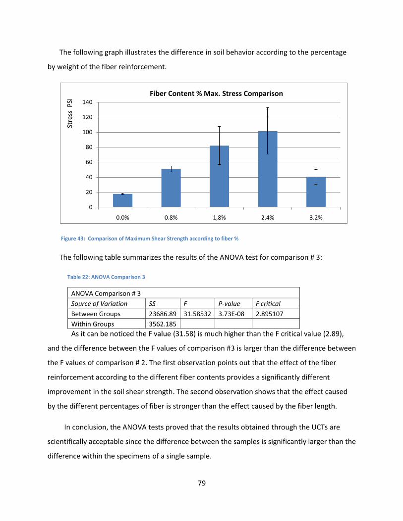
79

The following graph illustrates the difference in soil behavior according to the percentage

by weight of the fiber reinforcement.

Figure 43: Comparison of Maximum Shear Strength according to fiber %

The following table summarizes the results of the ANOVA test for comparison # 3:

Table 22: ANOVA Comparison 3

ANOVA Comparison # 3

Source of Variation SS F P-value F critical

Between Groups 23686.89 31.58532 3.73E-08 2.895107

Within Groups 3562.185 As it can be noticed the F value (31.58) is much higher than the F critical value (2.89),

and the difference between the F values of comparison #3 is larger than the difference between

the F values of comparison # 2. The first observation points out that the effect of the fiber

reinforcement according to the different fiber contents provides a significantly different

improvement in the soil shear strength. The second observation shows that the effect caused

by the different percentages of fiber is stronger than the effect caused by the fiber length.

In conclusion, the ANOVA tests proved that the results obtained through the UCTs are

scientifically acceptable since the difference between the samples is significantly larger than the

difference within the specimens of a single sample.

0

20

40

60

80

100

120

140

0.0% 0.8% 1,8% 2.4% 3.2%

Stre

ss P

SI

Fiber Content % Max. Stress Comparison

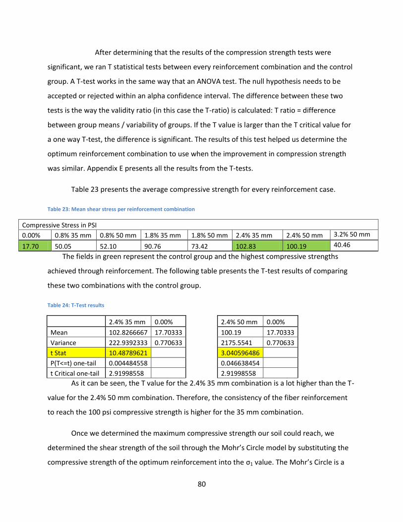
80

After determining that the results of the compression strength tests were

significant, we ran T statistical tests between every reinforcement combination and the control

group. A T-test works in the same way that an ANOVA test. The null hypothesis needs to be

accepted or rejected within an alpha confidence interval. The difference between these two

tests is the way the validity ratio (in this case the T-ratio) is calculated: T ratio = difference

between group means / variability of groups. If the T value is larger than the T critical value for

a one way T-test, the difference is significant. The results of this test helped us determine the

optimum reinforcement combination to use when the improvement in compression strength

was similar. Appendix E presents all the results from the T-tests.

Table 23 presents the average compressive strength for every reinforcement case.

Table 23: Mean shear stress per reinforcement combination

Compressive Stress in PSI

0.00% 0.8% 35 mm 0.8% 50 mm 1.8% 35 mm 1.8% 50 mm 2.4% 35 mm 2.4% 50 mm 3.2% 50 mm

17.70 50.05 52.10 90.76 73.42 102.83 100.19 40.46

The fields in green represent the control group and the highest compressive strengths

achieved through reinforcement. The following table presents the T-test results of comparing

these two combinations with the control group.

Table 24: T-Test results

2.4% 35 mm 0.00%

2.4% 50 mm 0.00%

Mean 102.8266667 17.70333

100.19 17.70333

Variance 222.9392333 0.770633

2175.5541 0.770633

t Stat 10.48789621

3.040596486

P(T<=t) one-tail 0.004484558

0.046638454

t Critical one-tail 2.91998558

2.91998558

As it can be seen, the T value for the 2.4% 35 mm combination is a lot higher than the T-

value for the 2.4% 50 mm combination. Therefore, the consistency of the fiber reinforcement

to reach the 100 psi compressive strength is higher for the 35 mm combination.

Once we determined the maximum compressive strength our soil could reach, we

determined the shear strength of the soil through the Mohr’s Circle model by substituting the

compressive strength of the optimum reinforcement into the σ1 value. The Mohr’s Circle is a

81

model created to represent the combinations of compressive and shear stresses acting on a

unit mass developed by the angle at which the compressive stresses (σ1, σ3) are acting. Figure

4444 presents Mohr’s Circle concept: the illustration shows a material cube subjected to

compressive stresses at angles 0 and θ, and the shear stresses developed due to the

compressive forces; the equations present how the stresses in the rotated position can be

translated into computations of the original stresses. Therefore, Mohr’s Circle represents all the

combinations of compressive and shearing stresses that can be generated from original stresses

through different inclined planes in the mass. Figure 4545 illustrates how Mohr’s Circle is

formed through the computation of the stress transformation for planes with angles 0 to 360.

Figure 44: Cube subjected to compressive and shear stresses. Li and Kapania, 2007.

Figure 45: Generation of Mohr's Circle through the transformation equations for angles 0-360. Li and Kapania, 2007.

Because σ1 and σ3 act perpendicular to each other, the plane where they develop the

highest shear strength is the 45: angle plane. In the Mohr’s Circle model, the compressive

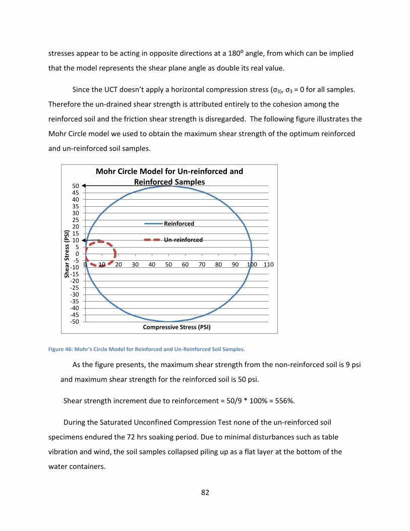
82

stresses appear to be acting in opposite directions at a 180: angle, from which can be implied

that the model represents the shear plane angle as double its real value.

Since the UCT doesn’t apply a horizontal compression stress (σ3), σ3 = 0 for all samples.

Therefore the un-drained shear strength is attributed entirely to the cohesion among the

reinforced soil and the friction shear strength is disregarded. The following figure illustrates the

Mohr Circle model we used to obtain the maximum shear strength of the optimum reinforced

and un-reinforced soil samples.

Figure 46: Mohr's Circle Model for Reinforced and Un-Reinforced Soil Samples.

As the figure presents, the maximum shear strength from the non-reinforced soil is 9 psi

and maximum shear strength for the reinforced soil is 50 psi.

Shear strength increment due to reinforcement = 50/9 * 100% = 556%.

During the Saturated Unconfined Compression Test none of the un-reinforced soil

specimens endured the 72 hrs soaking period. Due to minimal disturbances such as table

vibration and wind, the soil samples collapsed piling up as a flat layer at the bottom of the

water containers.

-50-45-40-35-30-25-20-15-10

-505

101520253035404550

0 10 20 30 40 50 60 70 80 90 100 110

She

ar S

tre

ss (

PSI

)

Compressive Stress (PSI)

Mohr Circle Model for Un-reinforced and Reinforced Samples

Reinforced

Un-reinforced

83

The optimal reinforced soil specimens had a significantly stronger structural integrity. All

three samples endured the 72 hrs soaking period. The average compressive strength of the

three cylinders equals 238.74 psi. From these results we conclude that the fibers are a great

addition for areas with intense rainfall events, as most of the tropical countries are.

These results prove that the implementation of fiber reinforcement can dramatically

reduce the risk of excessive weight induced landslides and enhance the bearing capacity of

footings in the reinforced area. We tested this last effect through a Bearing Capacity Test

described later in this chapter. The UCT did not provide information for us to predict how the

soil would behave under events that cause horizontal tensile stresses. As stated before, the

compressive loading method and the low height/diameter ratio of the cylindrical shape of the

samples allowed the fibers to behave as a mesh that forced the soil to remain structurally

sound forcing recompression. We decided to test the tensile strength of the soils samples to

determine the impact of the fibers in the soil tensile strength.

Indirect Tensile Test

The following table summarizes the indirect tensile strength results for each specimen

and the mean tensile strength per group.

Table 25: Indirect Tensile Test results

Spec # Non -Fiber 0.8% 35 mm 0.8% 50 mm 1.8% 35 mm 1.8% 50 mm 2.4% 35 mm 2.4% 50 mm

1 0.59 0.44 0.47 0.37 0.32 0.21 0.12

2 0.541 0.55 0.54 0.33 0.34 0.54 0.32

3 0.52 0.41 0.52 0.39 0.41 0.54 0.22

Average 0.55 0.47 0.51 0.36 0.36 0.43 0.22

We ran an ANOVA test among all the samples to determine if the fibers had a significant

impact on the soil tensile strength. The following table summarizes the test results. The F value

is much larger than the F critical value; therefore the test is scientifically valid because the

difference caused by the different fiber reinforcements between the samples is larger than the

differences caused by variations or errors within the specimens of each sample.

84

Table 26: ANOVA results for IIT

ANOVA Source of Variation SS F P-value F critical

Between Groups 0.840601 18.93579 7.29E-08 2.689628

Within Groups 0.332942

Total 1.173543

Figure 47 illustrates the behavior of the tensile strength of the soil as the fiber

reinforcement percent by weight is increased. The tensile strength of soil increases when the

cohesion and friction among its particles also increase. Therefore we had initially hypothesized

that if the fibers increased the soil shear strength they would increase the cohesion and friction

among the composite, so the soil shear strength would also increase. However, as Figure 47

illustrates, it is clear that the tensile strength of the soil decreases with an increase in fiber

percentage. We believe this occurs because the fibers do not allow the soil to compact as well

as when it is not reinforced. The more the soil is compacted the closer its particles come

together, developing stronger cohesion among particles. Contrary to what we predicted, the

fibers reduce the cohesion of the soil by increasing the distance between particles. The increase

in friction induced by the fibers does not compensate this loss. However, the decrease in tensile

strength from the un-reinforced sample to the optimum reinforcement sample is equal to a

22% decrease which is less than the shear strength increment. We had previously predicted

that the reinforcement of soil with fibers would increase the stability of a slope; however slope

stability depends both on the shear and tensile strength of the soil. As discussed in the UCT

Section, the shear strength information obtained through the UCT attributes all of its strength

to the soil cohesion. Therefore when modeling we cannot reflect the decrease of the soil tensile

strength due to the effect of the fiber on the compaction level.

85

Figure 47: Tensile Strength in PSI vs. Fiber % by weight

After characterizing the behavior of the soil under different types of stresses, we

wanted to obtain the bearing capacity of our soil. The bearing capacity is the maximum value of

load per unit area of footing that our soil can withstand without shear failure.

Bearing Capacity Test

The following images illustrate the results of the bearing capacity test with the 1:7

scaled down footing. The records of the relationship between the load increment and the

settlement obtained during the test do not show a clear capacity failure point. The main reason

why there was not a clear failure is because the need for enough space for the slip surface to

slide was not taking into account during the design phase. Therefore, even when the failure

surface might have developed, the testing device could not read a significant increase in

settlement because the soil could not slide.

We decided to use the total allowable settlement for a simple masonry walled structure as

the restraining parameter in order to determine the maximum allowable load. According to

Total Allowable Settlement Table, (Lambe & Whitman, 1969), a simple minimal structure like

the low income house, would have a maximum settlement of 1”. In our scaled down model, it

0

0.1

0.2

0.3

0.4

0.5

0.6

0 0.5 1 1.5 2 2.5 3

35 mm

50 mm

Fiber % vs Tensile StrengthTe

nsi

leSt

ren

gth

PSI

Fiber % by Weight

86

would be equivalent to 0.143”. Figure 48 illustrates the results of the BCT for the un-reinforced

soil, a maximum stress of 75 psi was achieved at a settlement of 0.15”.

Figure 48: Un-reinforced Stress vs Settlement Curve

87

Figure 49 illustrates the results of the BCT for the optimum reinforced soil, a maximum

stress of 100 psi was a achieved at a settlement of 0.15”.

Figure 49: Reinforced Soil: Stress vs Settlement Curve

It can be noticed that the bearing capacity of the un-reinforced soil obtained during the

test surpasses the predicted bearing capacity. However the bearing capacity of the reinforced

soil is 4 times less than the predicted bearing capacity. We believe this difference in behavior is

due to the lack of space for the failure surface to fully develop within the bearing box without

being intervened by the box. Despite this disparity with the predicted behavior, the fiber

reinforcement did significantly increment the bearing capacity of the soil. As Figure 4850 and

Figure 4951 illustrate, the fibers provide a 33% improvement in the bearing capacity. It is

important to notice that since the failure surface could not slide, the failure values for the un-

reinforced soil were probably inflated meanwhile the values for the reinforced were

underestimated since the effect of the fibers in the restriction of movement could not be

evaluated.

We decided to perform the second set of tests with a footing of a larger scale in order to

see if there was a significant difference in the soil bearing capacity and behavior. The new scale

0

100

200

300

400

500

600

0 0.1 0.2 0.3 0.4 0.5 0.6 0.7 0.8 0.9 1 1.1 1.2 1.3

Reinforced Soil: Stress vs Settlement Curve

Stre

ss (

PSI

)

Settlement (inches)

88

for the footing was selected based on the idea that Δσz < 20% σ’zd. We chose a scale of 1:4,

therefore the new maximum allowable settlement equals 1”/4 = 0.25”. Figure 50 illustrates the

dimensions of the new footing.

Figure 50: 1:4 scaled down footing

Figure 51 illustrates the results of the bearing capacity test on the un-reinforced soil. A

maximum allowable bearing capacity of 27 psi is attained at a settlement of 0.25”. It also

illustrates the results of the bearing capacity test on the reinforced soil. A maximum allowable

bearing capacity of 105 psi is attained at a settlement of 0.25”. This presents a bearing capacity

improvement of 289%.

Figure 51: 1:4 Scale Stress-Strain Curve. Results of Reinforced and Un-reinforced soils.

89

The results of the un-reinforced 1:4 BCT differ significantly from the un-reinforced 1:7

BCT. However, the results of the reinforced soil BCTs are consistent with each other. We believe

the difference between the un-reinforced samples is due to the effect of the box on the

influence zone of the footing in the 1:4 scale. Therefore we assumed the behavior of a footing

on the ground in a typical hillside would be more similar to the behavior of the 1:7 un-

reinforced soil BCT.

Modeling of Slope Stability with Soil Fiber Reinforcement

As described in the Methodology Chapter, we modeled seven different slope angles:

15°, 20°, 25°, 30°, 35°, 40° and 45°. The following table summarizes the factors of safety

obtained for the reinforced and the un-reinforced condition of each slope angle and presents

the percentage increment in factor of safety.

Table 27: Modeling Results

Degrees Slope Non Reinforced FS Reinforced FS % increment

15 26.79% 1.258 1.791 42.37%

20 36.40% 1.074 1.563 45.53%

25 46.63% 0.949 1.369 44.26%

30 57.74% 0.957 1.344 40.44%

35 70.02% 0.908 1.309 44.16%

40 83.91% 0.879 1.112 26.51%

45 100.00% 0.845 1.093 29.35%

The following figure illustrates the relationship between slope angle and percentage

improvement in the factor of safety of the hillside.

90

Figure 52: Slope angle vs Factor of Safety % Improvement.

As it can be noticed, there is not a clear pattern in the relationship, but a trend line can

be established which illustrates the effect slightly decreases with an increment in slope. As

established in the Background Chapter, most of the slopes in Rio de Janerio, Brazil vary

between 20° to 29°, therefore the modeling permits to imply that adding the reinforcement on

the top 3 ft of soil will improve the slope stability by at least 40%.

0.00%

10.00%

20.00%

30.00%

40.00%

50.00%

10 15 20 25 30 35 40 45

Angle vs % Increment

Angle in degrees

91

Chapter 5: Implementation of Reinforcement in Low-Income Communities

The implementation of the fiber reinforcement method does not require extensive

planning, design or heavy machinery and trained labor force. However, it does require an

anticipated plan, group collaboration, and complete understanding of each homeowner

responsibilities. The members of the community have to work together in: properly preparing

the fibers, adequately scheduling the use of the tools, developing terraces with enough space in

between houses and properly mixing and compacting of the soil. The development plan must

also include an area for growth of crops, enough spacing in-between housing to allow for the

easy removal of debris and most importantly a simple drainage path that prevents the

accumulation of water.

The reinforcement method is designed to significantly increase the stability of a slope for a

period of time significantly shorter than the house life-time. Therefore this method is a

temporary reinforcement that cannot be re-implemented once the housing has been

developed. We recommend the implementation of a permanent reinforcement method that

develops over time, such as planting trees that develop strong and distributed roots that can

hold the soil together throughout a period of 8 to 10 years. The proper implementation of this

method would have not only a positive impact on the economy of the community, through the

prevention of disasters, but it would also allow the population to live without fear every time

there is a strong nature event.

We believe the following procedures need to be applied to successfully implement the

reinforcement in a community.

1. Grading of the slope: As the results of the modeling process illustrate, a 20° slope has a

factor of safety of 1 when it is unreinforced and has been developed with the proposed

terraces. However, typically the houses are built directly on the slope, with no

significant grading, as the following figure illustrates.

92

Figure 53: Current Construction Methods in Low-Income Communities

The houses are typically built above slanted shallow foundations, which are built in

extreme proximity of the hill slope. The green element in the figure represents a typical-single-

room house with a slanted spread footing developed on a 20° slope. Under dry conditions this

scenario has a factor of safety of 1.063.

If instead the community developed in the manner suggested in the Modeling Section of

the Methodology Chapter so that the foundation of the house could be laid flat, a grading

procedure would be required. The grading procedure would entitle cutting 20 ft-long terraces

into the mountain, requiring removing a specific volume of soil per linear foot of mountain

perimeter. When comparing Figure 54 and Figure 55, it can be noticed that the steeper the final

slope is, the less amount of soil needs to be removed. As presented in the Modeling Section of

the Analysis and Results Chapter, with this development configuration, the slope has an

acceptable factor of safety when it has an angle of 20° or less. If the final slope in between

terraces equaled 25° after the grading process, a total removal of 320 cubic feet of soil per

linear foot of mountain perimeter would be required. Figure 54 illustrates the required

earthwork.

According to the results of the Modeling Analysis, if the fiber reinforcement was

implemented, the final slope could be as steep as 45° and still have an acceptable factor of

safety. If the final slope angle equaled 40° after the grading process, a total removal of 121

cubic feet of soil per linear foot of mountain perimeter would be requires. At optimum

conditions this would equal 16218 pounds of soil per liner foot of mountain. The grading with a

93

final slope angle of 25° requires 250% more earthwork than if the final slope has an angle of

40°.

It is important to minimize the amount of required grading due to the non-availability of

equipment; the fiber reinforcement permits the safe development on final slopes of even 45°.

Figure 54 illustrates the grading process that would be required if the slope was to remain

unreinforced. Therefore the final re-graded slope angle would equal 25° or less.

Figure 54: Slope Grading Method for 25 degrees

Figure 55: Required Grading Process for 40 degrees.

In intense rainfall conditions, the soil can achieve a moisture content of approximately 20%.

According to the UCT results and a saturated conditions slope stability model of the current

development practices with no terraces, the factor of safety of a 20° slope decreases from

1.063 on optimum conditions to 0.972 on saturated conditions.

94

In comparison, if the fiber reinforcement is implemented in this scenario, the factor of

safety for excessive rainfall would go from 1.44 when the soil is dry to 1. 124 when the soil is

saturated. A factor of safety of 1.124 is still safe; therefore we believe that if a community is not

able to implement the terraces system it should still try to reinforce the upper 3 ft layer of soil

to increase the stability of the slope. If instead only the recommended terraces system is

implemented with no fiber reinforcement, the slope factor of safety would go from 1.074 to

1.01. If both systems were implemented: the terraces and the fiber reinforcement the factor of

safety would go from 1.56 during optimum conditions to 1.12 during saturated conditions.

2. Drainage system

The reinforcement of soil with the fibers significantly increases the structural

integrity of the soil. In other words, the fibers behave as a mesh that keeps the soil from

sliding. We believe the reinforcement can significantly increase the erosion control.

In addition, we recommend cutting a draining fan between every two houses, to

prevent water accumulation. The fan consists of digging a homogenous opening in the

terrace ground. The opening should increase its opening and depth in the radial

direction in order to direct the water and mud downwards. The fan should gradually

increase its depth from 1 foot to 3 feet deep. This would permit most of the drainage

fan to be covered with the reinforced layer. The dimensions of the draining fan should

be designed according to the rain conditions of the area under study. To enhance this

mechanism we recommend slightly tilting the ground of each terrace towards the

draining fan. The following figure illustrates the drainage system suggestion.

95

Figure 56: Drainage System Suggestion

The suggested location for the housing and the drainage system allows for the growth of

crops in the remaining space between the housing

Cost and Schedule

We believe a community would require a minimal budget of $ 15,000.00 per

development of enough area for one house with its proper grading up and down. This estimate

does not include the costs of the labor because it is assumed the income provider for each

household is not involved in the ground preparation for the house. The workforce is provided

by the future inhabitants therefore there would be no charge. The following table presents the

estimated costs and duration of each procedure and the assumptions made to obtain such cost.

Drainin

g Fan

96

Table 28: Estimated costs for a 40 ft x 20 ft area stabilization.

Procedure Assumptions Cost Duration Workforce

per area

Excavation

for grading

The removed soil must be

transported to a far location.

The housing configuration is

identical to the housing

distribution diagram

presented in the analysis

section.

The working shifts are of 8.5

hrs per day.

We assumed each

homeowner should excavate

a distance of 40 ft, which

totals 40 x 121 = 4840 cu ft =

180 cu yards.

No cost

2.5 hours per cubic yard of

soil per person. The grading

process would take approx =

150 hours = 18 days of

excavation.

(Turtlesoft, 2010)

3 persons

Fiber

preparation

Cost of obtaining fiber equals

$1.00 per 2.7 lbs

Total volume of soil to be

reinforced = 40 ft x 3 ft deep x

(39 + 20) ft = 7086 ft3

Total weight of soil to be

reinforced = 7086 ft3

x 138

lbs/ft3

= 977888 lbs of soil

Total weight of required fiber

= 977888 x 0.024 = 23400 lbs

of fiber (Fao.org, 2003)

Total cost of fiber =

23400/2.7 = $8700.00

Total cost of coating = $10

per 70 lbs of fiber

23400/70 x 10 = $3340.00

Assuming a mechanical

cutting mechanism. Cutting

speed of 8 min per 20 lbs.

Coating and Drying time = 72

hours = 3.5 days

23400/20*8 = 9360 min =

156 hours = 18 days of work

= 6 days when working with 3

people.

3 persons

Soil mixing Assuming availability of

concrete mixer at $0.85 per

mix

Concrete mixer = 2 cu ft per

mix

Total cost of mixing =

7080/2x$0.85 = $3000.00

Mixing time = 5 min per 2 cu

ft Total time = 7080/2x5 =

17700 min = 295 hrs = 35

days = 12 days when working

with 3 people.

3 persons

Compaction The cohesive properties of the

soil require a machine with a

high impact ramming force so

it can push the air out.

Recommended rammer with

a frequency range of 500 to

750 blows per minute.

Assuming cost of diesel =

$2.50 per gallon

0.211 gallons of diesel per

hour

$2.5 *0.211 * 1.2 = $0.65

2183 sq ft / hour

40 ft x 20 ft + 39 ft x 40 ft =

2360 sq ft

2360/2183 = 1 hr 10 minutes

1 person

Total Cost & Duration $15040.00 36 days

Due to the low availability of labor force, some activities that could be initiated before

the previous activity has finished cannot be worked parallel.

97

Chapter 6: Conclusions and Recommendations

As the previous chapters present, the implementation of the optimum fiber

reinforcement on the upper 3 ft of a slope significantly increases the soil bearing capacity and

therefore its stability. A 25° to 30° slope can be fully developed for low income housing in an

inexpensive and safe manner by cutting terraces and reconfiguring the slope to a 40° angle, as

suggested in Chapter 5. A 30° to 45° slope can be reinforced to ensure safe development, it

must be noticed it will require extensive earthwork.

The positive effect of the fiber reinforcement was clearly established during the analysis

of the data obtained from the testing. However, the data obtained from the tests is not

accurate and extensive enough to establish the specific effect of the fibers on the soil. The time

constrains of the project guided the selection of simple testing and modeling methods whose

only purpose was to prove the positive relationship between the fiber reinforcement and soil

bearing capacity and slope stability. The following sections present the conclusions we obtained

from each major task accomplished during the project and recommendations on how to

improve its implementation.

Preparation of the fibers

During the handling of the fibers we concluded the fibers are a very flexible and strong

material. We recommend testing the initial moisture content of the fibers in order to increase

the precision in the measurement of the moisture content of the reinforced soil. It would also

be beneficial to observe the absorption capacity of the fiber and test any change in strength

and stiffness.

The fibers lengths vary significantly; therefore it is necessary to cut them to a desired length.

The fibers can be cut with scissors, paper cutters or hair-clippers, however large amounts of

fibers are necessary for the implementation of the fiber reinforcement on a hillside, therefore

we recommend a more mechanized system. We recommend finding a method to precisely

separate the desirable fiber length.

98

Testing Coated Fibers

The typical lifespan of a coconut fiber under burial conditions is between 2 and 3 years

therefore it was necessary to find a preservation process for the fibers that did not significantly

decrease the strength of the fibers. Another selection criterion was that the coating should

have no detrimental impacts onto the environment nor be a health hazard. We chose an all-

natural preservation coating recommended by the USDA. This coating is commonly used on

wood products to protect them from decay when exposed to the outdoor for 20 years. We

tested the effect of the coating on the fibers through a Tensile Strength Test and we decided to

implement it because the coating did not have a significant impact on the strength of the fibers.

We hypothesized that the coating would increase the service life of the fiber under burial

conditions to an acceptable period for a temporary reinforcement system. However, there has

been minimal research done to support our hypothesis, therefore the effects of the coating on

the preservation of fibers under burial conditions could not be determined. We strongly

recommended additional research on how the coating can affect the life of buried fibers over

long periods of time. In case the increment in useful life provided by the coating is not as we

predicted it, we recommend further research on other preservation methods that follow the

same two main criteria described above.

We propose the following preservation study to be followed through approximately one

to two years: Randomly selecting coir fibers, coating them, measuring their cross sectional area

and their tensile strength with a non-damaging procedure. We also recommend further study

into the effects of the coating on the strength and stiffness of the fibers.

We concluded that although we are not certain the fiber will be preserved for 10 years,

the tensile test strongly suggested that the coating process did not impact the fiber tensile

strength therefore it is an attractive solution.

Mixing the fibers into the soil

While combining the fibers with the soil we concluded the fibers would clump together

above the soil particles if the soil was not at its optimum moisture content or if large portions of

99

fibers were added to the soil. We recommend reaching the soil optimum moisture content

before adding the fibers and slowly adding the fibers to the soil.

To achieve the most homogenous mix we had to stir the fibers and the soil with

different movements. If a batter mixer was used the constant movement of the blade would

direct the fibers to the top of the soil and clump them together. For large amounts of soil we

recommend using a concrete mixer and for small amounts for testing we recommend mixing by

hand. We also recommend establishing a standard mixing procedure based around mixing time

and using the same number of mixes.

Shear Strength Test

The usage of the Unconfined Compression Test (UCT) to determine the effect of the

fiber on the shear strength of the soil leads us to the conclusion that the reinforcement

significantly improved the structural integrity of the soil. We concluded from the results that

the optimum reinforcement percentage by weight was around 2% and the length of the fibers

should be less than 50 mm to increase the consistency of the soil behavior. This test adapted

very well to our study’s short time frame and our inexperience in preparing soil samples.

However this test did not provide enough information as to determine the specific effect of the

fibers on the shear strength parameters of the soil.

We recommend testing the effect of the fiber reinforcement on the shear strength of

the soil through a triaxial test. This test would provide a variation of horizontal and vertical

compression stresses that would allow establishing the cohesion and friction angle of each soil

sample. This test would also allow performing tests on the un-drained and drained soil

conditions, allowing the modeling of the behavior of soil under almost complete saturation.

While performing the UCT we realized a complex recompression behavior was induced

by the presence of 1.8% or more fiber content. This behavior caused significant noise in the

data obtained from the test making it virtually impossible to determine the precise failure point

of each sample. We recognize the fibers behave as a mesh which will prevent the soil from

sliding but we believe that would not force the sample to remain in its cylindrical form.

100

Saturated Test

We realize testing of completely saturated soil is very important because this represents

one of the worst case scenarios for which urban planning should account for. During the

Saturated Tests we soaked the soil samples in water for 72 hrs and we let them cure for 72

hours inside plastic bags to prevent the excessive evaporation of water. We concluded the

samples were extremely fragile and difficult to handle once they were soaked. We also

concluded the soaking should take place in a no-vibration area because vibrations cause the soil

to collapse and slowly decrease its cross sectional area. When extruding the samples from the

soaking containers the bottom layer of the samples would separate and loose considerable

material. We recommend performing the soaking in tight containers that prevent vibration and

minimize the amount of manual handling.

Bearing Capacity

During the design and preparation of the bearing capacity test we concluded we had to

scale down all of the participating elements so that none of them would exert unexpected

pressures. Therefore we scaled down the fiber length to the same scale as we scaled down the

footing. However, the particle size had to remain the same. Therefore we recommend a study

of the scale effect of composite soils on the bearing capacity of a model. The main conclusion

from the test is that there is a clear and significant increment in the soil bearing capacity

induced by the fiber reinforcement. We designed the soil container for the test based on a

solution for Boussinesq Model of the influence zone under a uniformly distributed load.

According to this solution and the scale for our model, the box should have not interfered with

the slip surface. However, none of the tests presented a clear failure point. Therefore we

conclude our design failed to provide enough space for considerable sliding of the slip surface

to occur. We recommend designing a soil container significantly larger than the one used in this

test or determine the bearing capacity of the soil through another testing procedure. Previous

studies that have used similar bearing tests procedures have used soil containers of similar

dimensions but constructed out of stiff and apparent materials. These designs allowed the

performers to clearly determine failure when a visible slip surface crack could be seen through

101

the soil walls. Based on our resources we concluded failure would be determined when a

maximum settlement of 1”/our scale factor was achieved. These approached provided

consistent results but they were not accurate enough.

Modeling of Slope Stability with Soil Fiber Reinforcement

We modeled the effects of reinforcing the upper 3 ft of soil in a slope using a 2-

dimension simple software that calculated the factor of safety of the slopes using Bishop’s

method. The software assumed all the elements in the model were soils with different unit

weights and shear strengths. We concluded the implementation of the reinforcement increased

the factor of safety of the slope by an average of 39%. The modeling provides only a basic idea

of the real effect. We recommend modeling the implementation of the reinforcement in a low

income community using a three dimensional software that allows the inclusion of unit loads

and distributed loads, developed by the activities of the population, the accumulation of

resources, etc. We also recommend the software allows inputting different saturation levels

and erosion efforts into the model. Lastly we recommend modeling using software that allows

for the inclusion of GIS data. Therefore the model can run in real circumstances taking into

account surrounding loads.

102

Bibliography

Alexander, David. "On the Causes of Landslides: Human Activities, Perception, and Natural

Processes." Environmental Geology Volume 20.Number 3 (November 1992): 165 to 179.

Springer Link <http://www.springerlink.com/content/x144p415334p6367/>.

American Concrete Institute. ACI 318-05; “ Building Code Requirements for Structural

Concrete and Commentary.” 2005

Arnold Verruijt, Delft “Slope Stability Bishop’s” Software STB 2006

Autralian Government Geoscience Australia. "Natural Hazards: Landslides." 2009.

<http://www.ga.gov.au/hazards/landslide/>.

Babu, Sivkumar G. L., and A. K. Vasudevan. "

Strength and Stiffness Response of Coir Fiber-Reinforced Tropical Soil." 20.9 (2008): 571-

577-577.

Brown, Lance. Building with Reinforced Soil. Vol. 644.000-3. Abbotsford, BC: Ministry if

Agriculture and Land, 2006.

Coduto, Donald P. (1998). Geotechnical Engineering: Principles and Practices. Prentice-Hall

Day, Robert. Geotechnical and Foundation Engineering: Design and Construction. Illustrated

ed. McGraw-Hill Professional, 1999.

Delgado, Jim'nez C., and I. C. Guerrero.

The Selection of Soils for Unstabilised Earth Building: A Normative Review. Vol. 0950-

0618/$. Madrid, Sp: Construction and Building Materials-Science Direct, 2005.

Department of Sustainability and Environment, Victoria AU. "What Causes Bushfires on Public

Land in Victoria?" 2009. <http://www.dse.vic.gov.au/DSE/nrenfoe.nsf/childdocs/-

44688EB30B57BF124A2567CB000DB2EF-

BDFD9C1B8EF2DDC5CA256BE600287703?open>.

Department of Transportation: Initial Study on Reinforced Earth, Department of Transportation,

2009.

Dieckow, J., et al. "Land use, Tillage, Texture and Organic Matter Stock Composition in

Tropical and Subtropical Brazilian Soils." European Journal of Soil Science 60 (2009):

240-9. .

Fernandes, Nelson F., et al. "Geomorphic Impacts of Rapid Environmental Change." Volume

55.Issue 2 (2004): 163-81.

103

Fred, Wayne W. "Fiber Reinforced Soil and Method." 1988.

<http://www.freepatentsonline.com/4790691.html>.

French, Matthew A. Adobe with Sawn Timber Roof Framing and Corrugated Iron Sheeting. Vol.

136. http://www.world-housing.net: World Housing Encyclopedia, 2007. Adobe / Earthen

House <http://www.world-housing.net/>.

GeotechniCAL Project. "Building Foundations: Bearing Capacity." 2002.

<http://environment.uwe.ac.uk/geocal/foundations/founbear.htm>.

Ginzburg, L. K., E. L. Korchagina, and V. B. Shvets. "Reinforcement of Foundations in Weak

Saturated Silty-Clayey Soils." Soil Mechanics and Foundation Engineering 32.6 (1995):

207, Springerlink: <http://www.springerlink.com/content/bkv86442826t0270/>.

Holtz, Robert D. "Geosynthetics for Soil Reinforcement." 1 (2001): 3-20. Abstract.

Islam, Mohammad S., and Kazuyoshi Iwashita. "Performance of Composite Soil Reinforced with

Jute Fiber." Adobe USA(2009) Abstract.

Lambe, William, and Robert Whitman. "Chapter 14: Shallow Foundations." Illustrated ed.John

Wiley and Sons, 1969. 200-200-210.

Li, Jing, and Rakesh K. Kapania. "Mohr's Circle for 2d Stress Analysis." 2007.

<http://www.aoe.vt.edu/~jing/java/nsfapplets/MohrCircles2-3D/Theory/theory.htm>.

Marandi, S. M., et al.

“Strength and Ductility of Randomly Distributed Palm Fibers Reinforced Silty-Sand Soils."

American Journal of Applied Science 5.3 (2008): 209-220.

Military Soils Engineering Science; "Chapter 5: Soil Classification." FM5-410. FM: FM

Science-Engineering, 2000. 5-11. <http://www.itc.nl/~rossiter/Docs/FM5-410/FM5-

410_Ch5.pdf>

National Society of Professional Engineers. “ Code of Ethics for Engineers.” Publication #1102

2003

O'Meara Sheehan, Molly. State of the World 2003: Uniting Divided Cities, 2003.

OEA. Unidad de Desarrollo Sostenible y Medio Ambiente. “Códigos de construcción en la

región Centroamericana.” “Central American Building Code” Doc# 8445 1996.

Pereira, M. L., et al. "Toxic Effects Caused by Stainless Steel Corrosion Products on Mouse

Seminiferous Cells." 77 (1994): 73-80. Abstract.

104

Peter Hintereder, ed. Tatsachen Über Deutschland. 2008th ed. http://www.tatsachen-ueber-

deutschland.de/de/head-navi/wir-ueber-uns.html: Societäts-Verlages, Frankfurt am Main

Frankfurter Societäts-Druckerei GmbH.

Plonsky, M. "Analysis of Variance, One Way." 2009.

<http://www.uwsp.edu/psych/stat/12/anova-1w.htm>.

Rivero, Yensi. "Venezuela's Vargas Disaster Hard to Forget." Tierramerica2004: 1.

Sassa, Kyoji, and Paolo Canuti, “Landslides - Disaster Risk Reduction” Ed. Kyoji Sassa and

Paolo Canuti. Illustrated ed.Springer, 2008. 50 - 62.

Shah, Anup. "Poverty Around The World." 2009. <http://www.globalissues.org/article/4/poverty-

around-the-world>.

"Poverty Facts and Stats." 2009. <http://www.globalissues.org/article/26/poverty-facts-and-

stats>.

Smith, Christopher. "Basement Construction in Clay Soils." 2007.

<http://www.buzzle.com/articles/basement-construction-in-clay-soils.html>.

The CIA World Factbook, "Brazil." 2010. <https://www.cia.gov/library/publications/the-world-

factbook/geos/br.html>.

The National Lime Association, Lime-Treated Soil Construction Manual: Lime Stabilization &

Lime Modification, The National Lime Association, 2003.

Tsuchida, T, and K. Mizuno. "New Slip Circle Method for Analysis for Bearing Capacity and

Slope Stability", Foundation Design Codes, Ed. Yusuke Hondo, et al. 1st ed. Netherlands:

A.A. Balkema, 2002. 339-340.

UN-HABITAT, "Brazilian Habitat" 2010:

<http://www.unhabitat.org/categories.asp?catid=140>.

United National Enviromental Program, Enviromental Assement Program for Asia and the

Pacific, "Asia- Pacific Enviromental Outlook." 1996.

<http://www.rrcap.unep.org/apeo/Chp1h-nathazards.html>.

United Nations Human Settlements Programme. The Challenge of Slums: Global Report on

Human Settlements, Vol. 1844070379. UN-HABITAT, 2003.

Unknown. "Coconut Palm Tree." 2003. <http://coconutpalmtree.net/>.

Venezuelan Government. "La reconstruccion de Vargas es un Hecho." 2007.

<http://estadovargas.gob.ve/ochoanos.php>.

105

Ward Harris, Charles, Nicholas Dines, and Kyle Brown. "Sliding Risk." Time-Saver Standards

for Landscape Architecture: Design and Construction Data. 2nd ed.McGraw-Hill

Professional, 1998.

106

Appendix A

Devastating Effects of Natural Disasters on Low Income Settlements

Poverty affects every country around the world forcing low standards of living and

hazardous conditions. It is internationally recognized that people living in poverty are people

that earn less than the minimum daily income that facilitates their survival. Almost half the

world lives on less than $2.50 a day. Most of the poverty is concentrated in developing

countries, where more than 1.1 billion people have inadequate access to water, shelter and

basic sanitation. Only 25% of these households have access to piped water. These minimal

resources cause communities to develop inadequate housing settlements. Urban slum growth

is outpacing urban growth by a wide margin. The probability of natural events to become

natural disasters is especially high in these communities. Some of the main reasons are

construction on hazardous locations, unsustainable practices and that the vast majority of the

structures are non-engineered construction; therefore they do not have systems to resist

extreme vibrations, horizontal displacements, etc (Shah [2], 2009).

Low income settlements constantly sustain great damage and casualties from natural

events such as droughts, earthquakes and tropical storms. Fires get triggered by thunderstorms

during dry seasons, the lightning strikes dry flammable materials located in the nearby areas.

These fires spread rapidly through the combustible materials that are part of the houses, such

as dry palm leaves and bamboo used as roofing (DSE, Victoria AU, 2009). Since these

settlements do not have proper fire prevention systems to extinguish the fire, great

percentages of the settlements get destroyed. Flood disasters occur because most of these

housing units are closely built drastically increasing the amount of impervious surface.

Therefore the rain water is unable to be absorbed and recharge the groundwater table,

becoming runoff. Most of these communities do not have drainage systems because of

inadequate planning, therefore the runoff accumulates in-between the clustered areas creating

flooding and destruction. Earthquakes experienced in these communities cause large areas of

the communities to collapse. This happens because most of the structures are non-engineered

construction, therefore they do not include a horizontal resistance frame that can withstand

107

seismic forces which results in the collapse of the structures. Landslides are easily triggered in

these areas because the environment within and surrounding the communities has been worn

down through unsustainable development practices. Common landslide triggers are

earthquakes, intense rainfall events, volcanic activity and excess material accumulation. Low

income communities in developing countries tend to build their housing in landslide prone

hillsides because of their proximity to cities with employment opportunities (UNEP, 1996).

The disaster that has been minimally addressed for low income settlements is landslides

on hillsides. As previously mentioned, the countries with the highest frequency of landslide

disasters are the developing nations. Additionally, these countries are divided by their high

educational disparity, which doesn’t allow the least educated groups to understand and

evaluate the consequences of unsustainable developing practices (Sassa & Canuti, 2008).

Examples of these activities are clearing the vegetative cover in order to grow crops and raise

livestock and developing settlements on hillsides without adequate environmental planning

(Alexander, 1992).

Landslides are caused when the stability of a slope changes from stable to an unstable

condition. Landslides are mass movements of rock, soil, and debris down a slope under the

influence of gravity (Cruden, 1991). The size and rate of each landslide can vary tremendously,

and as a result so can the risks to life and property. Landslides can be devastating to any

community as they can cause property damage injury and death and adversely affect a variety

of resources such as water supplies, fisheries, sewage disposal system, dams and roadways can

be affected years after a landslide occurs. Figure 1 (Chapter 1) illustrates the various types of

landslides such as rock falls, creep, earth flows, slumps, block slides, and debris flows. All types

of landslides can occur slowly over time or abruptly. Sudden events are extremely dangerous

because of the fast speed of the material and the momentum it carries. Meanwhile gradual

events might move only millimeters per year and remain active for long periods. Even though

this last type of landslide is not life-threatening it causes considerable damage to structures

(Geosciences Australia, 2009). Therefore we can conclude that the most dangerous landslides

are the ones that occur abruptly.

108

As mentioned in the Introduction, one of the worst abrupt landslides that have recently

occurred is the Tragedy of Vargas in 1999. This tragedy happened in one of the Venezuela’s

poorest states, where most of the inhabitants live on hill slopes. The insufficiency of the

structures built on the slopes caused vast structural failure killing thousands of people. The

tragedy was triggered by excessive rainfall during a tropical storm. The mudslides generated

were particularly large because of the excess eroded-material produced by the community’s

deforestation activities, the insufficient drainage system and the development of houses to

close to the slope (Venezuelan Government, 2007).

Brazil suffers many of these natural disasters and the majority of them occur in low

income housing settlements. This is often the case in other developing countries where the

slum areas are so poorly constructed. Many slum settlements are being developed in Brazil

because of the poor economical circumstances and the increasing population of this country.

Brazil is one of the world’s most populated countries with approximately 196 million

inhabitants (The CIA World Fact book, 2010). The country has 6.3 million inadequate housing

units of which 3.2 million are in the slums (National Housing Plan, 2009). In Brazil, despite the

existence of a few support programs and the housing development support from municipalities,

there is no integrated and comprehensive approach at the national level to the problem of

informal land and housing markets. In terms of distribution of income, Brazil is among the worst

in the world. There are 38 million inhabitants living in rural areas and 73 percent have an

annual income below the poverty line. Of the total wealth of Brazil 75 % go to the richest 10%

Brazilian people (UN-HABITAT, 2005).

The area with the most frequent landslides occurrence within Brazil is Serra do Mar, a

long coast range that runs from the south to the southeastern regions of the country. The

topography of this area is well known for its deep cuts and odd landforms. Due to the low costs

of establishing housing in unwanted territories, many settlements were built upon the hillsides

in and around cities along Serra do Mar, since the 1960’s. These communities are

internationally known as the slums of Rio de Janeiro. Nowadays, these hillsides are densely

populated, severely affecting the slope stability through the extensive usage of cuts, landfills,

109

deforestations, changes in drainage conditions and accumulation of trash deposits on hill

slopes. These factors add to the weight of the materials above the slope failure surface,

increasing the probability of slope failure to occur. In addition, these conditions cause the water

from the intense summer rainstorms to not drain properly which recently has caused the

erosion of large amounts of soil in the deforested areas and a significant increase in the

occurrence of landslides. In a ten-year period starting in 1986 through 1996 there were 123

deaths and 414 houses destroyed from landslides in Rio de Janeiro, Serra do Mar (Fernandez, et

al, 2003).

The soil at the base of the steep slopes in Rio de Janeiro is made of an upper layer of

clay soil with an approximate content of 40% clay which lies over a sandy silt saprolite soil. This

configuration has caused two main concerns among experts. The first one is that clayey soils

significantly vary their moisture content because they hold moisture according to the weather

conditions. This can cause structures to sink when moisture content decreases drastically and

to crack when moisture content increases drastically. A way to avoid this is through proper

ground compaction, so the ground does not shift under the weight of the home (Smith, 2007).

The second concerning factor is the steepness of the hillsides on which these settlements are

constructed (Fernandez, et al, 2003). A recent field study establishes that the slope angles of

the hills in Serra do Mar vary from 20: to 29: (Cruz O. and Colangelo, 2000). A study by Zhou et

al (2002) observed that landslide potential is very high for slopes with threshold angles of 25˚ to

30˚ and a study by GAO (1993) presents that the landslide potential increases rapidly for hill

slopes above 31˚.

Brazil became the focus area for our project because of the amount of in-depth

documentation of the slums, the country’s natural disasters and its geological characteristics. In

addition, the situation in Brazil is representative of the situation in most third world countries

around the world. If in the long term a cost effective and easily constructible slope stability

method is implemented in these areas it would be beneficial to many people

110

Appendix B

Practices in Adobe Construction

Table B 1 shows the areas of the world where the majority of the population lives in

earth-built structures (French, 2007).

Table B 1: World distribution of Earth Construction. Copyright De Sensi, 2003

Traditional adobe construction is done by preparing adobe blocks, which typically have

dimensions: 7.9“ wide, 15.8” long and 3.95” deep (French, 2007). The soil used to prepare

adobe must have a minimum of 10% by weight content of clay so it would have enough

cohesion, also known as dry strength. However, if the content exceeds 25% by weight, the

blocks will obtain too much dry strength which will cause excessive micro cracks that

significantly decrease the compressive strength of the blocks.

Most of the low income adobe housing found in highlands has a basic vertical and

horizontal structure of timber poles, a timber roof frame and a concrete or stones strip footing

foundation. Typically each terrace on the hillside holds 10 or fewer building units and the

number of occupants in each unit is 5 or less. Each house consists of one or two rooms,

therefore all the walls in the unit act as bearing walls and they form the vertical load-resisting

system. Table B 2 illustrates the typical wall configuration for a single room adobe house.

111

Table B 2: Typical low income house detail. Copyright French, 2007.

Each wall is typically 1.5 ft thick and 10 ft tall. The dimensions of a one room, one story

building is usually: between 10 and 20 ft long and between 8 and 16 ft wide. The walls

dimensions and the adobe blocks dimensions act as the lateral load resistance system.

However, the structures do not have a load resistance path that can withstand seismic forces.

Table B 3illustrates the traditional design of a low income single room adobe house.

Table B 3: Single-room low income house in Guatemala. Copyright French, 2007.

When preparing adobe mix, it is also recommended to add straw and a small amount of

coarse aggregate because this helps control the micro cracking caused by drying shrinkage so it

improves the strength of the blocks (Delgado and Guerrero, 2005). Therefore we hypothesized

112

that if the soil used for the project was within the range of perfect soils for adobe and

presented a significant increase in cohesion and tensile strength when reinforced with fibers,

then the fibers would have a positive impact on the strength of the adobe blocks.

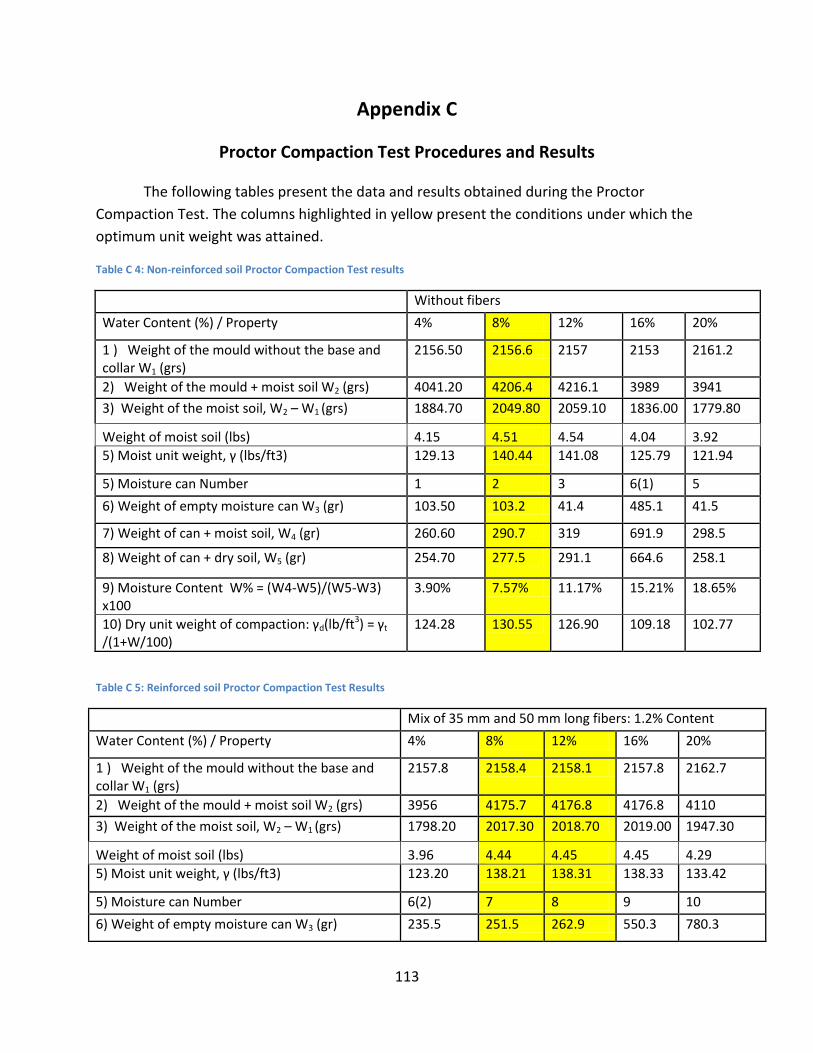
113

Appendix C

Proctor Compaction Test Procedures and Results

The following tables present the data and results obtained during the Proctor

Compaction Test. The columns highlighted in yellow present the conditions under which the

optimum unit weight was attained.

Table C 4: Non-reinforced soil Proctor Compaction Test results

Without fibers

Water Content (%) / Property 4% 8% 12% 16% 20%

1 ) Weight of the mould without the base and collar W1 (grs)

2156.50 2156.6 2157 2153 2161.2

2) Weight of the mould + moist soil W2 (grs) 4041.20 4206.4 4216.1 3989 3941

3) Weight of the moist soil, W2 – W1 (grs) 1884.70 2049.80 2059.10 1836.00 1779.80

Weight of moist soil (lbs) 4.15 4.51 4.54 4.04 3.92

5) Moist unit weight, γ (lbs/ft3) 129.13 140.44 141.08 125.79 121.94

5) Moisture can Number 1 2 3 6(1) 5

6) Weight of empty moisture can W3 (gr) 103.50 103.2 41.4 485.1 41.5

7) Weight of can + moist soil, W4 (gr) 260.60 290.7 319 691.9 298.5

8) Weight of can + dry soil, W5 (gr) 254.70 277.5 291.1 664.6 258.1

9) Moisture Content W% = (W4-W5)/(W5-W3) x100

3.90% 7.57% 11.17% 15.21% 18.65%

10) Dry unit weight of compaction: γd(lb/ft3) = γt /(1+W/100)

124.28 130.55 126.90 109.18 102.77

Table C 5: Reinforced soil Proctor Compaction Test Results

Mix of 35 mm and 50 mm long fibers: 1.2% Content

Water Content (%) / Property 4% 8% 12% 16% 20%

1 ) Weight of the mould without the base and collar W1 (grs)

2157.8 2158.4 2158.1 2157.8 2162.7

2) Weight of the mould + moist soil W2 (grs) 3956 4175.7 4176.8 4176.8 4110

3) Weight of the moist soil, W2 – W1 (grs) 1798.20 2017.30 2018.70 2019.00 1947.30

Weight of moist soil (lbs) 3.96 4.44 4.45 4.45 4.29

5) Moist unit weight, γ (lbs/ft3) 123.20 138.21 138.31 138.33 133.42

5) Moisture can Number 6(2) 7 8 9 10

6) Weight of empty moisture can W3 (gr) 235.5 251.5 262.9 550.3 780.3

114

7) Weight of can + moist soil, W4 (gr) 384.5 455.3 489 796.8 999

8) Weight of can + dry soil, W5 (gr) 379.1 441.1 472.4 766.5 965.5

9) Moisture Content W% = (W4-W5)/(W5-W3) x100

3.76% 7.49% 7.92% 14.01% 18.09%

10) Dry unit weight of compaction: γd(lb/ft3) = γt /(1+W/100)

118.74 128.58 128.15 121.32 112.98

115

Appendix D

Sample Data Tables per UCT sample and Stress-Strain Curves per UCT specimen.

0.8% 35 mm Table D 1: 0.8% 35 mm - Summary of Results

Specimen # Max. Stress (PSI)

1 45.72

2 49.34

3 55.09

Average 50.05

Variance 22.33

Stad. Dev. 4.73

Table D 2: 0.8% 35 mm - Data for Specimen 1

Extension (in) ∆H (in) Axial Strain є Corrected Area, Ac Load (Lbs) Stress (psi) Time (Min)

-0.060468 0 0.00% 12.56637 1.538653 0.12244212 0.085317

-0.058468 0.002 0.04% 12.57139856 2.564421 0.20398852 0.089183

-0.054468 0.006 0.13% 12.58272755 3.59019 0.28532685 0.097117

-0.050668 0.0098 0.21% 12.59281491 4.103074 0.32582659 0.10485

-0.048668 0.0118 0.26% 12.59912773 5.128842 0.40707913 0.108817

-0.044868 0.0156 0.34% 12.60924142 7.180379 0.56945369 0.116483

-0.042868 0.0176 0.39% 12.61557073 6.154611 0.48785831 0.120533

-0.039068 0.0214 0.47% 12.62571084 8.719032 0.69057751 0.1281

-0.037168 0.0233 0.51% 12.63078701 9.7448 0.7715117 0.131883

-0.033268 0.0272 0.60% 12.64222334 12.309222 0.97365959 0.139717

-0.029068 0.0314 0.69% 12.65368039 13.33499 1.0538428 0.148317

-0.027168 0.0333 0.73% 12.65877909 15.89941 1.25599869 0.152117

-0.023368 0.0371 0.81% 12.66898881 18.976715 1.49788711 0.159783

-0.021368 0.0391 0.86% 12.67537825 21.028253 1.65898426 0.16375

-0.017568 0.0429 0.94% 12.68561478 21.541137 1.69807592 0.1714

-0.015568 0.0449 0.98% 12.69073924 24.618443 1.93987462 0.175383

-0.011768 0.0487 1.07% 12.70228444 28.721517 2.26113005 0.183017

-0.007868 0.0526 1.15% 12.71256449 32.824591 2.58205896 0.190867

-0.005968 0.0545 1.19% 12.71771076 33.337475 2.62134244 0.19465

-0.002168 0.0583 1.28% 12.72930511 39.492085 3.10245411 0.202417

-0.000268 0.0602 1.32% 12.73446494 41.543621 3.26229812 0.206283

0.003832 0.0643 1.41% 12.74608987 45.646697 3.58123138 0.214117

0.005632 0.0661 1.45% 12.75126332 47.698232 3.74066716 0.217917

0.009532 0.07 1.53% 12.76162283 54.365726 4.26009503 0.225667

116

0.013232 0.0737 1.61% 12.77199919 61.033224 4.77867428 0.23315

0.015132 0.0756 1.66% 12.77849298 62.571874 4.89665519 0.23695

0.019032 0.0795 1.74% 12.7888968 69.239368 5.41402195 0.244717

0.020932 0.0814 1.78% 12.79410507 73.342444 5.7325185 0.248517

0.024932 0.0854 1.87% 12.80583919 81.548587 6.36807833 0.256367

0.026932 0.0874 1.91% 12.81106127 84.113013 6.56565535 0.26025

0.031332 0.0918 2.01% 12.82413512 92.832047 7.23885441 0.26905

0.035132 0.0956 2.09% 12.83461342 101.03819 7.87232055 0.276733

0.037132 0.0976 2.14% 12.84117106 107.1928 8.34758742 0.2807

0.040832 0.1013 2.22% 12.85167723 115.39895 8.97929102 0.2882

0.042832 0.1033 2.26% 12.85693677 119.50202 9.2947507 0.292

0.046832 0.1073 2.35% 12.86878648 129.24682 10.043435 0.29985

0.048732 0.1092 2.39% 12.87406003 132.83701 10.318191 0.30365

0.052632 0.1131 2.48% 12.88594135 143.60758 11.144516 0.3115

0.056532 0.117 2.56% 12.89652094 152.8395 11.8512197 0.319267

0.058432 0.1189 2.60% 12.90181725 158.48123 12.2836362 0.32315

0.062232 0.1227 2.69% 12.91374987 168.7389 13.0666074 0.33075

0.064232 0.1247 2.73% 12.91906035 176.43217 13.6567339 0.334533

0.068132 0.1286 2.82% 12.9310249 185.66409 14.3580339 0.342217

0.070032 0.1305 2.86% 12.9363496 193.87024 14.9864718 0.346017

0.073832 0.1343 2.94% 12.94701216 204.6408 15.8060251 0.353783

0.077732 0.1382 3.03% 12.95902857 214.89849 16.5829164 0.36155

0.079632 0.1401 3.07% 12.96437635 221.0531 17.0508088 0.36535

0.083432 0.1439 3.15% 12.97508518 234.90097 18.1040024 0.373033

0.085432 0.1459 3.19% 12.98044623 241.05559 18.5706704 0.377

0.089232 0.1497 3.28% 12.99252481 252.33904 19.4218632 0.384683

0.091032 0.1515 3.32% 12.99790029 259.51942 19.9662572 0.3883

0.094932 0.1554 3.40% 13.0086646 271.31575 20.8565409 0.396067

0.098832 0.1593 3.49% 13.02079577 283.62498 21.7824611 0.40385

0.100632 0.1611 3.53% 13.02619467 287.72803 22.0884179 0.40765

0.104532 0.165 3.61% 13.03700591 300.03726 23.0142769 0.415317

0.106432 0.1669 3.65% 13.04241827 308.24341 23.6339153 0.4193

0.110232 0.1707 3.74% 13.05461251 317.98821 24.3583028 0.426883

0.112232 0.1727 3.78% 13.06003949 325.1686 24.89798 0.430867

0.116032 0.1765 3.86% 13.07090701 337.99071 25.8582444 0.438533

0.119832 0.1803 3.95% 13.08315461 350.81281 26.8140845 0.446133

0.121732 0.1822 3.99% 13.08860535 355.42878 27.155588 0.449933

0.125532 0.186 4.07% 13.09952048 367.2251 28.0334765 0.457517

0.127532 0.188 4.12% 13.10635169 371.84106 28.3710579 0.4615

0.131232 0.1917 4.20% 13.11729645 384.66317 29.3248818 0.4691

0.133232 0.1937 4.24% 13.12277569 391.33066 29.8207229 0.47315

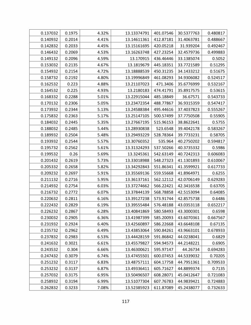
117

0.137032 0.1975 4.32% 13.13374791 401.07546 30.5377763 0.480817

0.140932 0.2014 4.41% 13.14611361 412.87181 31.4063781 0.488667

0.142832 0.2033 4.45% 13.15161695 420.05218 31.939204 0.492467

0.146432 0.2069 4.53% 13.16263748 427.23254 32.4579736 0.499883

0.149132 0.2096 4.59% 13.170915 436.46446 33.1385074 0.5052

0.153032 0.2135 4.67% 13.1819679 445.18351 33.7721589 0.51295

0.154932 0.2154 4.72% 13.18888539 450.31235 34.1433212 0.51675

0.158732 0.2192 4.80% 13.19996849 461.08293 34.9306082 0.524517

0.162532 0.223 4.88% 13.21107023 471.3406 35.6776999 0.532167

0.164532 0.225 4.93% 13.2180183 474.41791 35.8917575 0.53615

0.168332 0.2288 5.01% 13.22915044 485.18849 36.67571 0.543733

0.170132 0.2306 5.05% 13.23472354 488.77867 36.9315359 0.547417

0.173932 0.2344 5.13% 13.24588384 495.44616 37.4037823 0.555267

0.175832 0.2363 5.17% 13.25147105 500.57499 37.7750508 0.55905

0.184032 0.2445 5.35% 13.27667195 515.96153 38.8622641 0.5755

0.188032 0.2485 5.44% 13.28930838 523.6548 39.4042178 0.583267

0.189932 0.2504 5.48% 13.29493229 528.78364 39.7733231 0.58705

0.193932 0.2544 5.57% 13.30760352 535.964 40.2750202 0.594817

0.195732 0.2562 5.61% 13.31324293 537.50266 40.3735332 0.5986

0.199532 0.26 5.69% 13.3245361 542.63149 40.7242313 0.606083

0.201432 0.2619 5.73% 13.33018988 548.27323 41.1301893 0.610067

0.205332 0.2658 5.82% 13.34292843 551.86341 41.3599921 0.617733

0.209232 0.2697 5.91% 13.35569136 559.55668 41.8964971 0.6255

0.211132 0.2716 5.95% 13.36137161 562.12112 42.0706149 0.629283

0.214932 0.2754 6.03% 13.37274662 566.22421 42.3416538 0.63705

0.216732 0.2772 6.07% 13.37844139 568.78858 42.5153094 0.64085

0.220632 0.2811 6.16% 13.39127238 573.91744 42.8575738 0.6486

0.222432 0.2829 6.19% 13.39555484 576.48188 43.0353118 0.652217

0.226232 0.2867 6.28% 13.40841869 580.58493 43.3000301 0.6598

0.230032 0.2905 6.36% 13.41987399 585.20093 43.6070361 0.667567

0.231932 0.2924 6.40% 13.42560897 586.22668 43.6648108 0.67135

0.235732 0.2962 6.49% 13.43853064 590.84261 43.9663101 0.678933

0.237832 0.2983 6.53% 13.44428159 591.86842 44.0238041 0.6829

0.241632 0.3021 6.61% 13.45579827 594.94573 44.2148221 0.6905

0.243532 0.304 6.66% 13.46300621 595.97147 44.26734 0.694283

0.247432 0.3079 6.74% 13.47455501 600.07453 44.5339032 0.70205

0.251232 0.3117 6.83% 13.48757111 604.17758 44.7951361 0.709533

0.253232 0.3137 6.87% 13.49336411 605.71627 44.8899374 0.7135

0.257032 0.3175 6.95% 13.50496507 608.28071 45.0412647 0.721083

0.258932 0.3194 6.99% 13.51077304 607.76783 44.9839421 0.724883

0.262832 0.3233 7.08% 13.52385923 611.87089 45.2438077 0.732633

118

0.264732 0.3252 7.12% 13.52968346 613.40951 45.3380532 0.736433

0.268532 0.329 7.20% 13.54134698 614.9482 45.4126311 0.7442

0.272332 0.3328 7.29% 13.5544925 614.43532 45.3307508 0.751783

0.274332 0.3348 7.33% 13.56034315 615.46107 45.3868359 0.75575

0.278032 0.3385 7.41% 13.57205962 615.97394 45.3854433 0.763233

0.279932 0.3404 7.45% 13.57792545 617.51263 45.479159 0.767017

0.283832 0.3443 7.54% 13.59114212 620.58994 45.661353 0.774783

0.285732 0.3462 7.58% 13.59702445 621.10281 45.6793185 0.778583

0.289632 0.3501 7.67% 13.61027835 620.077 45.5594648 0.786417

0.293432 0.3539 7.75% 13.6220813 622.12856 45.670595 0.794

0.295432 0.3559 7.79% 13.62799046 621.61569 45.6131582 0.798133

0.299332 0.3598 7.88% 13.64130482 623.66718 45.7190267 0.805717

Figure D 1: 0.8% 35 mm Spec. 1 - Stress vs Strain Curve

0

5

10

15

20

25

30

35

40

45

50

0.00% 5.00% 10.00% 15.00% 20.00% 25.00% 30.00% 35.00%

Tru

e S

tre

ss P

SI

Strain %

0.8% 35 mm Spec. 1 - Stress vs Strain Curve

119

Figure D 2: 0.8% 35mm Spec. 2 - Stress vs Strain Curve

0.8% 50 mm Table D 3: 0.8% 50mm - Summary of Results

Specimen # Stress (PSI)

1 49.63

2 50.60

3 56.06

Average 52.10

Variance 12.02

Stand. Dev. 3.47

Table D 4: 0.8% 50 mm - Data for Specimen 1

Extension (in) ∆H (in) Axial Strain є

Corrected Area, Ac Load (Lbs) Stress (psi) Time (Min)

-0.113667 0 0.00% 12.56637 -2.051537 -0.1632561 0.0059

-0.108167 0.0055 0.12% 12.58146776 -1.538653 -0.1222952 0.01715

-0.104267 0.0094 0.21% 12.59281491 -0.512884 -0.0407283 0.024983

-0.102367 0.0113 0.25% 12.59786466 1.538653 0.12213602 0.028933

-0.098266 0.0154 0.34% 12.60924142 1.025768 0.08135049 0.036933

-0.096467 0.0172 0.38% 12.61430436 2.051537 0.16263576 0.040717

-0.092567 0.0211 0.46% 12.62444244 4.103074 0.32501031 0.048383

-0.088767 0.0249 0.55% 12.63586727 5.128842 0.40589553 0.056133

-0.086666 0.027 0.59% 12.64095161 5.128842 0.40573227 0.0601

-0.082866 0.0308 0.67% 12.65113259 4.615958 0.3648652 0.067767

05

10152025303540455055

0.00% 5.00% 10.00% 15.00% 20.00% 25.00% 30.00%

Tru

e S

tre

ss P

SI

Strain %

0.8% 35 mm Spec. 2 - Stress vs Strain Curve

120

-0.080867 0.0328 0.72% 12.65750403 6.154611 0.48624207 0.071733

-0.077067 0.0366 0.80% 12.66771169 7.693263 0.60731276 0.079467

-0.072967 0.0407 0.89% 12.67921501 7.180379 0.56631101 0.087383

-0.071067 0.0426 0.93% 12.68433431 8.719032 0.68738586 0.091267

-0.067266 0.0464 1.02% 12.69586785 8.206148 0.64636369 0.0991

-0.065466 0.0482 1.06% 12.70100061 11.283453 0.88839087 0.1027

-0.061466 0.0522 1.14% 12.71127858 11.283453 0.88767254 0.11055

-0.059566 0.0541 1.18% 12.7164238 12.822106 1.00831069 0.114417

-0.055567 0.0581 1.27% 12.7280158 13.33499 1.04768805 0.122417

-0.051566 0.0621 1.36% 12.73962895 15.89941 1.24802771 0.130267

-0.049567 0.0641 1.40% 12.74479716 15.89941 1.24752162 0.134133

-0.045266 0.0684 1.50% 12.75773604 17.950947 1.40706368 0.142817

-0.043367 0.0703 1.54% 12.76291895 20.002485 1.56723435 0.146683

-0.039566 0.0741 1.62% 12.77329742 22.054021 1.72657226 0.154183

-0.035766 0.0779 1.71% 12.78499339 24.105559 1.88545729 0.161933

-0.033866 0.0798 1.75% 12.79019847 25.644211 2.00498929 0.165733

-0.029866 0.0838 1.83% 12.80062137 26.669979 2.08349097 0.17365

-0.027866 0.0858 1.88% 12.80714431 27.182863 2.12247651 0.177517

-0.024066 0.0896 1.96% 12.81759486 32.311705 2.52088675 0.185267

-0.022166 0.0915 2.00% 12.82282653 32.311705 2.51985823 0.189067

-0.018266 0.0954 2.09% 12.83461342 34.363243 2.67738824 0.1969

-0.014466 0.0992 2.17% 12.84510886 37.953431 2.95469905 0.204483

-0.012667 0.101 2.21% 12.85036302 38.466317 2.99340314 0.208167

-0.008866 0.1048 2.29% 12.86088425 43.595161 3.38974834 0.215933

-0.006867 0.1068 2.34% 12.86746877 45.133811 3.50759048 0.219717

-0.002966 0.1107 2.42% 12.87801804 47.698232 3.70384883 0.227483

0.000734 0.1144 2.51% 12.88990666 51.801304 4.01874935 0.235067

0.002634 0.1163 2.55% 12.89519754 55.90438 4.33528683 0.238867

0.006434 0.1201 2.63% 12.90579234 58.468802 4.53043102 0.246617

0.008333 0.122 2.67% 12.91109627 62.571874 4.84636414 0.250417

0.012734 0.1264 2.77% 12.92437519 68.726486 5.31758673 0.259133

0.014634 0.1283 2.81% 12.92969441 68.726486 5.3153991 0.262917

0.018534 0.1322 2.89% 12.940346 76.419752 5.90554163 0.270783

0.022334 0.136 2.98% 12.95235003 79.497051 6.13765462 0.278367

0.024333 0.138 3.02% 12.95769231 82.061478 6.33303184 0.28235

0.028134 0.1418 3.10% 12.96839009 91.293393 7.03968591 0.290017

0.030234 0.1439 3.15% 12.97508518 91.806275 7.07558168 0.294

0.034034 0.1477 3.23% 12.98581172 100.525309 7.74116483 0.301667

0.037934 0.1516 3.32% 12.99790029 107.192798 8.24693186 0.309433

0.039733 0.1534 3.36% 13.00328022 110.782988 8.5196186 0.313067

0.043434 0.1571 3.44% 13.01405344 117.450486 9.02489655 0.320667

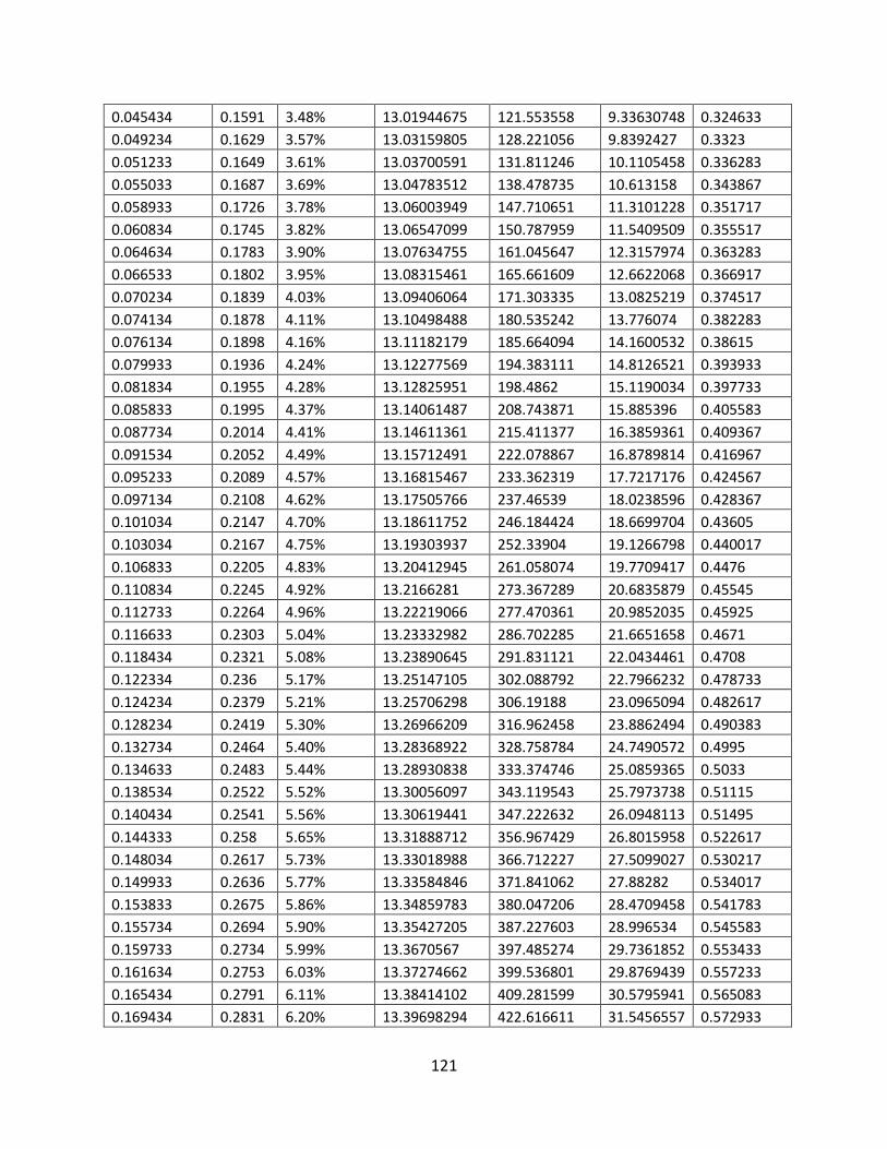
121

0.045434 0.1591 3.48% 13.01944675 121.553558 9.33630748 0.324633

0.049234 0.1629 3.57% 13.03159805 128.221056 9.8392427 0.3323

0.051233 0.1649 3.61% 13.03700591 131.811246 10.1105458 0.336283

0.055033 0.1687 3.69% 13.04783512 138.478735 10.613158 0.343867

0.058933 0.1726 3.78% 13.06003949 147.710651 11.3101228 0.351717

0.060834 0.1745 3.82% 13.06547099 150.787959 11.5409509 0.355517

0.064634 0.1783 3.90% 13.07634755 161.045647 12.3157974 0.363283

0.066533 0.1802 3.95% 13.08315461 165.661609 12.6622068 0.366917

0.070234 0.1839 4.03% 13.09406064 171.303335 13.0825219 0.374517

0.074134 0.1878 4.11% 13.10498488 180.535242 13.776074 0.382283

0.076134 0.1898 4.16% 13.11182179 185.664094 14.1600532 0.38615

0.079933 0.1936 4.24% 13.12277569 194.383111 14.8126521 0.393933

0.081834 0.1955 4.28% 13.12825951 198.4862 15.1190034 0.397733

0.085833 0.1995 4.37% 13.14061487 208.743871 15.885396 0.405583

0.087734 0.2014 4.41% 13.14611361 215.411377 16.3859361 0.409367

0.091534 0.2052 4.49% 13.15712491 222.078867 16.8789814 0.416967

0.095233 0.2089 4.57% 13.16815467 233.362319 17.7217176 0.424567

0.097134 0.2108 4.62% 13.17505766 237.46539 18.0238596 0.428367

0.101034 0.2147 4.70% 13.18611752 246.184424 18.6699704 0.43605

0.103034 0.2167 4.75% 13.19303937 252.33904 19.1266798 0.440017

0.106833 0.2205 4.83% 13.20412945 261.058074 19.7709417 0.4476

0.110834 0.2245 4.92% 13.2166281 273.367289 20.6835879 0.45545

0.112733 0.2264 4.96% 13.22219066 277.470361 20.9852035 0.45925

0.116633 0.2303 5.04% 13.23332982 286.702285 21.6651658 0.4671

0.118434 0.2321 5.08% 13.23890645 291.831121 22.0434461 0.4708

0.122334 0.236 5.17% 13.25147105 302.088792 22.7966232 0.478733

0.124234 0.2379 5.21% 13.25706298 306.19188 23.0965094 0.482617

0.128234 0.2419 5.30% 13.26966209 316.962458 23.8862494 0.490383

0.132734 0.2464 5.40% 13.28368922 328.758784 24.7490572 0.4995

0.134633 0.2483 5.44% 13.28930838 333.374746 25.0859365 0.5033

0.138534 0.2522 5.52% 13.30056097 343.119543 25.7973738 0.51115

0.140434 0.2541 5.56% 13.30619441 347.222632 26.0948113 0.51495

0.144333 0.258 5.65% 13.31888712 356.967429 26.8015958 0.522617

0.148034 0.2617 5.73% 13.33018988 366.712227 27.5099027 0.530217

0.149933 0.2636 5.77% 13.33584846 371.841062 27.88282 0.534017

0.153833 0.2675 5.86% 13.34859783 380.047206 28.4709458 0.541783

0.155734 0.2694 5.90% 13.35427205 387.227603 28.996534 0.545583

0.159733 0.2734 5.99% 13.3670567 397.485274 29.7361852 0.553433

0.161634 0.2753 6.03% 13.37274662 399.536801 29.8769439 0.557233

0.165434 0.2791 6.11% 13.38414102 409.281599 30.5795941 0.565083

0.169434 0.2831 6.20% 13.39698294 422.616611 31.5456557 0.572933

122

0.171234 0.2849 6.24% 13.40269838 425.181012 31.7235381 0.57655

0.175034 0.2887 6.32% 13.41414389 435.95159 32.4993972 0.584133

0.176933 0.2906 6.36% 13.41987399 440.567552 32.829485 0.588

0.180834 0.2945 6.45% 13.43278461 448.260823 33.3706552 0.595767

0.184734 0.2984 6.53% 13.44428159 458.518494 34.1050945 0.603617

0.186634 0.3003 6.58% 13.4514772 463.647329 34.4681348 0.6074

0.190634 0.3043 6.66% 13.46300621 471.853473 35.0481509 0.61525

0.192534 0.3062 6.70% 13.46877814 476.982342 35.4139282 0.619033

0.196234 0.3099 6.79% 13.48178307 487.752886 36.178663 0.626617

0.198034 0.3117 6.83% 13.48757111 490.317321 36.3532705 0.630233

0.201934 0.3156 6.91% 13.4991621 501.087899 37.1199261 0.638067

0.205933 0.3196 7.00% 13.51222581 508.781135 37.653392 0.645917

0.207833 0.3215 7.04% 13.51804002 512.884224 37.9407239 0.649717

0.211634 0.3253 7.12% 13.52968346 522.629022 38.6283259 0.6573

0.213634 0.3273 7.17% 13.53697081 527.757857 38.9864073 0.661267

0.217334 0.331 7.25% 13.5486469 536.476908 39.5963458 0.66885

0.221333 0.335 7.34% 13.5618066 544.683051 40.1630157 0.6766

0.223233 0.3369 7.38% 13.56766357 548.273233 40.410291 0.6804

0.226833 0.3405 7.46% 13.5793927 556.99225 41.0174639 0.687817

0.228834 0.3425 7.50% 13.58526486 560.069558 41.2262524 0.691783

0.232734 0.3464 7.59% 13.59849583 569.301516 41.8650359 0.699367

0.234633 0.3483 7.63% 13.60438454 571.865883 42.0354101 0.70315

0.238434 0.3521 7.71% 13.61617727 580.07206 42.6016824 0.710917

0.242334 0.356 7.80% 13.62946855 585.200929 42.9364452 0.7185

0.244333 0.358 7.84% 13.63538411 589.816858 43.2563434 0.722467

0.248134 0.3618 7.92% 13.64723067 596.997221 43.7449352 0.73005

0.250034 0.3637 7.96% 13.65316167 598.535908 43.8386304 0.73385

0.253834 0.3675 8.05% 13.66652529 605.203398 44.2836336 0.7415

0.257633 0.3713 8.13% 13.67842604 613.922381 44.882531 0.749083

0.259733 0.3734 8.18% 13.68587454 615.973942 45.0080074 0.753067

0.263433 0.3771 8.26% 13.69780903 623.154305 45.4929912 0.76065

0.265434 0.3791 8.30% 13.70378408 625.205866 45.6228632 0.764617

0.269133 0.3828 8.38% 13.71574984 630.847609 45.9943945 0.7722

0.271034 0.3847 8.42% 13.72174055 634.43779 46.2359558 0.775983

0.274933 0.3886 8.51% 13.73523882 640.079533 46.6012671 0.78375

0.278634 0.3923 8.59% 13.7472596 642.6439 46.747055 0.791167

0.280534 0.3942 8.63% 13.75327788 646.747023 47.0249368 0.79495

0.284434 0.3981 8.72% 13.7668383 649.824331 47.2021474 0.802717

0.286434 0.4001 8.76% 13.77287374 654.440259 47.5166092 0.8065

0.290333 0.404 8.85% 13.78647285 656.49182 47.6185481 0.81435

0.294334 0.408 8.93% 13.79858351 663.15931 48.0599555 0.822267

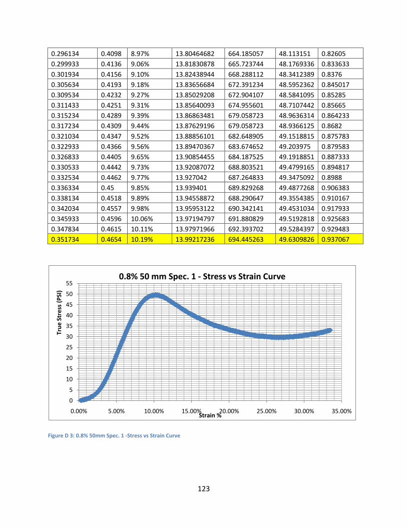
123

0.296134 0.4098 8.97% 13.80464682 664.185057 48.113151 0.82605

0.299933 0.4136 9.06% 13.81830878 665.723744 48.1769336 0.833633

0.301934 0.4156 9.10% 13.82438944 668.288112 48.3412389 0.8376

0.305634 0.4193 9.18% 13.83656684 672.391234 48.5952362 0.845017

0.309534 0.4232 9.27% 13.85029208 672.904107 48.5841095 0.85285

0.311433 0.4251 9.31% 13.85640093 674.955601 48.7107442 0.85665

0.315234 0.4289 9.39% 13.86863481 679.058723 48.9636314 0.864233

0.317234 0.4309 9.44% 13.87629196 679.058723 48.9366125 0.8682

0.321034 0.4347 9.52% 13.88856101 682.648905 49.1518815 0.875783

0.322933 0.4366 9.56% 13.89470367 683.674652 49.203975 0.879583

0.326833 0.4405 9.65% 13.90854455 684.187525 49.1918851 0.887333

0.330533 0.4442 9.73% 13.92087072 688.803521 49.4799165 0.894817

0.332534 0.4462 9.77% 13.927042 687.264833 49.3475092 0.8988

0.336334 0.45 9.85% 13.939401 689.829268 49.4877268 0.906383

0.338134 0.4518 9.89% 13.94558872 688.290647 49.3554385 0.910167

0.342034 0.4557 9.98% 13.95953122 690.342141 49.4531034 0.917933

0.345933 0.4596 10.06% 13.97194797 691.880829 49.5192818 0.925683

0.347834 0.4615 10.11% 13.97971966 692.393702 49.5284397 0.929483

0.351734 0.4654 10.19% 13.99217236 694.445263 49.6309826 0.937067

Figure D 3: 0.8% 50mm Spec. 1 -Stress vs Strain Curve

0

5

10

15

20

25

30

35

40

45

50

55

0.00% 5.00% 10.00% 15.00% 20.00% 25.00% 30.00% 35.00%

Tru

e S

tre

ss (

PSI

)

Strain %

0.8% 50 mm Spec. 1 - Stress vs Strain Curve

124

Figure D 4: 0.8% 50mm Spec. 2 -Stress vs Strain Curve

Figure D 5: 0.8% 50mm Spec. 3 - Stress vs Strain Curve

1.8% 35 mm Table D 5: 1.8% 35 mm - Summary of Results

Specimen # Max. Stress (PSI) Strain %

1 64.87 8.66%

2 93.66 11.56%

0

5

10

15

20

25

30

35

40

45

50

55

0.00% 5.00% 10.00% 15.00% 20.00% 25.00% 30.00% 35.00%

Tru

e S

tre

ss (

PSI

)

Strain %

0.8% 50 mm Spec. 2 - Stress vs Strain Curve

0

10

20

30

40

50

60

0.00% 5.00% 10.00% 15.00% 20.00% 25.00% 30.00% 35.00%

Tru

e S

tre

ss (

PSI

)

Strain %

0.8% 50mm Spec. 3 -Stress vs Strain Curve

125

3 113.76 14.94%

Average 90.76 11.72%

Variance 603.94 0.10%

Std. Dev. 24.58 3.14%

Table D 6: 1.8% 35mm - Data for Specimen 1

Extension (in) ∆H (in)

Axial Strain є

Corrected Area, Ac Load (Lbs) Stress (psi) Time (Min)

-0.076456 0 0.00% 12.56637 4.615958 0.367326284 0.005617

-0.069756 0.0067 0.15% 12.58524787 9.7448 0.774303383 0.019083

-0.067856 0.0086 0.19% 12.59029155 11.796337 0.936939145 0.022867

-0.063956 0.0125 0.27% 12.60039106 15.89941 1.261818774 0.030717

-0.062056 0.0144 0.32% 12.60671148 20.515369 1.627337077 0.034483

-0.058056 0.0184 0.40% 12.61683735 23.592673 1.869935575 0.042317

-0.056156 0.0203 0.44% 12.62190639 28.208633 2.234894804 0.046267

-0.052156 0.0243 0.53% 12.63332663 33.337475 2.638851664 0.054183

-0.050256 0.0262 0.57% 12.63840893 34.876127 2.759534621 0.057983

-0.046256 0.0302 0.66% 12.64985907 42.056507 3.324662098 0.065967

-0.044256 0.0322 0.71% 12.65622923 44.108043 3.485085661 0.06995

-0.040456 0.036 0.79% 12.66643484 48.211119 3.806210637 0.077767

-0.038456 0.038 0.83% 12.67154381 50.262654 3.966576981 0.081733

-0.034556 0.0419 0.92% 12.6830541 54.365726 4.286485383 0.089217

-0.032656 0.0438 0.96% 12.68817649 54.365726 4.284754868 0.093017

-0.028656 0.0478 1.05% 12.69971703 59.49457 4.684716192 0.101

-0.026556 0.0499 1.09% 12.7048529 63.08476 4.965406567 0.105133

-0.024656 0.0518 1.13% 12.70999292 65.649182 5.165162751 0.108917

-0.020656 0.0558 1.22% 12.72157319 68.726486 5.402357472 0.116783

-0.018856 0.0576 1.26% 12.72672676 72.316672 5.682267985 0.120583

-0.014956 0.0615 1.35% 12.73833756 75.39398 5.918667147 0.128433

-0.013056 0.0634 1.39% 12.74350472 77.445515 6.077253999 0.132317

-0.009056 0.0674 1.48% 12.75514616 82.574359 6.473807351 0.1405

-0.007156 0.0693 1.52% 12.76032697 85.651667 6.712341087 0.144367

-0.003156 0.0733 1.61% 12.77199919 91.806275 7.188089637 0.152233

-0.001356 0.0751 1.64% 12.77589467 95.909347 7.507055236 0.156017

0.002644 0.0791 1.73% 12.7875954 100.525309 7.861158087 0.163883

0.004544 0.081 1.77% 12.79280261 103.602609 8.09850759 0.167667

0.008544 0.085 1.86% 12.80453434 109.757225 8.571746703 0.175517

0.010444 0.0869 1.90% 12.80975535 115.911832 9.048715515 0.1794

0.014344 0.0908 1.99% 12.82151821 121.040676 9.440432404 0.18725

0.016244 0.0927 2.03% 12.82675309 123.605094 9.636506851 0.19105

126

0.018144 0.0946 2.07% 12.83199224 127.195284 9.912356681 0.19475

0.022044 0.0985 2.16% 12.84379599 134.888554 10.50223424 0.202533

0.023944 0.1004 2.20% 12.84904908 140.017389 10.89710127 0.206333

0.027844 0.1043 2.28% 12.85956815 147.197778 11.44655685 0.214183

0.029744 0.1062 2.33% 12.86615133 152.839503 11.87919364 0.217983

0.033644 0.1101 2.41% 12.87669843 162.071411 12.58641039 0.225833

0.035544 0.112 2.45% 12.88197847 164.635828 12.78032162 0.229617

0.039444 0.1159 2.54% 12.89387441 175.91928 13.64363219 0.237483

0.041344 0.1178 2.58% 12.89916855 178.996588 13.87659889 0.241283

0.045144 0.1216 2.66% 12.90976988 190.79293 14.7789567 0.248867

0.047144 0.1236 2.71% 12.91640456 195.921765 15.16844444 0.252817

0.051444 0.1279 2.80% 12.9283642 204.640799 15.82882381 0.261467

0.053344 0.1298 2.84% 12.9336867 209.769652 16.21885985 0.265433

0.057244 0.1337 2.93% 12.94567838 223.617521 17.27352669 0.273283

0.059144 0.1356 2.97% 12.95101515 227.207702 17.54362105 0.277083

0.061144 0.1376 3.01% 12.95635633 235.413863 18.16975831 0.28095

0.065044 0.1415 3.10% 12.96839009 246.184424 18.98342217 0.288717

0.066944 0.1434 3.14% 12.97374561 251.31326 19.37091011 0.2926

0.070744 0.1472 3.22% 12.98446993 264.135365 20.34240646 0.300017

0.072744 0.1492 3.27% 12.99118164 270.802872 20.84513014 0.304067

0.076544 0.153 3.35% 13.00193482 284.137851 21.85350527 0.31175

0.078444 0.1549 3.39% 13.00731808 291.318247 22.39648828 0.315717

0.082244 0.1587 3.48% 13.01944675 305.1661 23.43925252 0.323317

0.084244 0.1607 3.52% 13.02484453 311.320716 23.90206772 0.327367

0.088144 0.1646 3.60% 13.03565353 325.681476 24.98390091 0.334967

0.090144 0.1666 3.65% 13.04241827 333.887619 25.60013122 0.339017

0.093844 0.1703 3.73% 13.05325647 347.222632 26.60046042 0.3466

0.095644 0.1721 3.77% 13.05868232 355.941649 27.25708767 0.350233

0.099444 0.1759 3.85% 13.06954758 371.328189 28.41170949 0.358

0.101344 0.1778 3.89% 13.07498699 376.457024 28.79215285 0.3618

0.105144 0.1816 3.98% 13.08724224 391.843531 29.94087859 0.369567

0.107144 0.1836 4.02% 13.0926964 399.536801 30.51600594 0.373367

0.109144 0.1856 4.06% 13.0981551 409.281599 31.24727078 0.37725

0.113044 0.1895 4.15% 13.11045383 422.616611 32.23508632 0.3851

0.114944 0.1914 4.19% 13.11592736 432.361409 32.96460839 0.388883

0.118844 0.1953 4.28% 13.12825951 448.260823 34.14472595 0.396733

0.120844 0.1973 4.32% 13.13374791 454.415405 34.59906556 0.4006

0.124544 0.201 4.40% 13.14473849 470.314819 35.77970145 0.40825

0.126444 0.2029 4.44% 13.15024069 479.033869 36.42776436 0.41205

0.130244 0.2067 4.53% 13.16263748 492.881722 37.4455137 0.419633

0.132244 0.2087 4.57% 13.16815467 503.6523 38.24775093 0.4236

127

0.136044 0.2125 4.65% 13.17920294 518.525933 39.34425591 0.431183

0.137944 0.2144 4.69% 13.18473403 526.219203 39.91124902 0.434983

0.141844 0.2183 4.78% 13.19719597 541.092836 41.00059114 0.442817

0.143844 0.2203 4.82% 13.20274217 549.299013 41.60491857 0.446617

0.147644 0.2241 4.91% 13.2152382 562.633992 42.57463874 0.454383

0.149444 0.2259 4.95% 13.22079958 570.840136 43.17742906 0.458

0.151344 0.2278 4.99% 13.22636565 578.020499 43.7021412 0.461783

0.155244 0.2317 5.07% 13.23751185 591.355478 44.67270622 0.46955

0.157144 0.2336 5.12% 13.24448777 599.048782 45.2300453 0.473333

0.160944 0.2374 5.20% 13.25566456 613.922381 46.31396475 0.480917

0.162944 0.2394 5.24% 13.26126003 620.589938 46.79720757 0.484883

0.166744 0.2432 5.33% 13.27386712 632.386229 47.64144642 0.492483

0.168744 0.2452 5.37% 13.27947797 641.618153 48.31651926 0.49645

0.173144 0.2496 5.47% 13.29352586 654.953132 49.26857921 0.50555

0.174944 0.2514 5.50% 13.29774603 662.133495 49.79291178 0.509167

0.178844 0.2553 5.59% 13.31042262 674.955601 50.70880317 0.516817

0.180844 0.2573 5.63% 13.31606443 681.110217 51.14951349 0.5208

0.184644 0.2611 5.72% 13.32877599 692.393702 51.94728328 0.528383

0.186544 0.263 5.76% 13.33443336 698.035445 52.34833953 0.532167

0.190344 0.2668 5.84% 13.34576253 710.344677 53.22623382 0.539933

0.192344 0.2688 5.89% 13.35285304 717.52504 53.73571009 0.543717

0.194244 0.2707 5.93% 13.35853088 723.679656 54.17359607 0.547517

0.198144 0.2746 6.01% 13.36990105 731.885766 54.74130011 0.555267

0.200044 0.2765 6.05% 13.3755934 737.527509 55.13979731 0.559067

0.203844 0.2803 6.14% 13.38841892 747.272306 55.8148285 0.566733

0.205844 0.2823 6.18% 13.39412705 754.452669 56.32712502 0.570517

0.209544 0.286 6.26% 13.40555793 764.197467 57.0060173 0.5781

0.211644 0.2881 6.31% 13.41271214 768.813463 57.31976167 0.582067

0.215444 0.2919 6.39% 13.42417477 778.045387 57.95852635 0.58965

0.217344 0.2938 6.43% 13.42991343 780.609754 58.12470481 0.593617

0.221144 0.2976 6.52% 13.44284339 789.328805 58.71739945 0.6012

0.223044 0.2995 6.56% 13.44859803 794.970547 59.11177843 0.605

0.226844 0.3033 6.64% 13.46012211 801.125163 59.51841719 0.612767

0.228744 0.3052 6.68% 13.46589156 806.253965 59.87379013 0.616383

0.232444 0.3089 6.76% 13.4774453 813.434395 60.35523623 0.623967

0.234444 0.3109 6.81% 13.48467647 816.511703 60.55107848 0.627933

0.238144 0.3146 6.89% 13.49626249 821.640505 60.87911419 0.635517

0.240144 0.3166 6.93% 13.50206296 826.769374 61.23281874 0.6393

0.242044 0.3185 6.97% 13.50786843 829.846682 61.43431781 0.643267

0.245944 0.3224 7.06% 13.520949 836.514172 61.86800734 0.65085

0.247944 0.3244 7.10% 13.52677072 839.078607 62.03096247 0.654817

128

0.251744 0.3282 7.19% 13.53988794 843.181662 62.27390253 0.6624

0.253644 0.3301 7.23% 13.54572599 846.771843 62.51210483 0.6662

0.257544 0.334 7.31% 13.5574172 852.413586 62.87433466 0.673867

0.259444 0.3359 7.36% 13.56473446 853.952206 62.95384615 0.67765

0.263344 0.3398 7.44% 13.57645851 857.029514 63.12614686 0.685417

0.265144 0.3416 7.48% 13.58232815 861.132636 63.40095945 0.6892

0.269044 0.3455 7.57% 13.59555339 865.748565 63.67880292 0.696867

0.271044 0.3475 7.61% 13.60143955 865.748565 63.65124528 0.70085

0.274844 0.3513 7.69% 13.61322717 870.364493 63.93520671 0.708433

0.276844 0.3533 7.74% 13.62060481 870.364493 63.900576 0.7124

0.280544 0.357 7.82% 13.63242569 873.954742 64.10852785 0.719983

0.282344 0.3588 7.86% 13.63834382 875.493362 64.19352476 0.7236

0.284344 0.3608 7.90% 13.6442671 877.544923 64.3160176 0.7274

0.288044 0.3645 7.98% 13.6561291 878.057797 64.29770768 0.73515

0.289944 0.3664 8.02% 13.66206784 879.596417 64.38237807 0.73895

0.293844 0.3703 8.11% 13.67544891 884.212413 64.65692052 0.746717

0.295844 0.3723 8.15% 13.68140446 885.23816 64.70374897 0.7505

0.299644 0.3761 8.24% 13.69482345 885.23816 64.64034846 0.758083

0.301644 0.3781 8.28% 13.7007959 887.289721 64.76191073 0.76205

0.305444 0.3819 8.36% 13.71275644 886.263907 64.63061683 0.769633

0.307344 0.3838 8.40% 13.71874454 887.802594 64.71456563 0.773433

0.311244 0.3877 8.49% 13.73223691 890.367029 64.83772706 0.781167

0.313144 0.3896 8.53% 13.73824205 889.341215 64.73471729 0.784967

0.317144 0.3936 8.62% 13.75177282 891.905649 64.85750317 0.792733

0.319044 0.3955 8.66% 13.75779505 892.418523 64.86639172 0.796517

129

Appendix E

Results of Statistical T-Test

Table E 1: T-Test Calculations and Results

T -Test: Paired Two Sample for Means

0.8% 35 mm 0.00%

0.8% 50 mm 0.00%

1.8% 35 mm 0.00%

Mean 50.05 17.70

52.10 17.70

90.76 17.70

Variance 22.33 0.77

12.02 0.77

603.85 0.77

Observations 3.00 3.00

3.00 3.00

3.00 3.00

Pearson Correlation 0.27

0.50

0.04

Hypothesized Mean Difference 0.00

0.00

0.00

df 2.00

2.00

2.00

t Stat 12.27

19.10

5.15

P(T<=t) one-tail 0.00

0.00

0.02

t Critical one-tail 2.92

2.92

2.92

P(T<=t) two-tail 0.01

0.00

0.04

t Critical two-tail 4.30

4.30

4.30

2.4% 35 mm 0.00%

2.4% 50 mm 0.00%

3.2% 50 mm 0.00%

Mean 102.83 17.70

100.19 17.70

40.46 17.70

Variance 222.94 0.77

2175.55 0.77

102.25 0.77

Observations 3.00 3.00

3.00 3.00

3.00 3.00

Pearson Correlation 1.00

-0.39

-0.48

Hypothesized Mean Difference 0.00

0.00

0.00

df 2.00

2.00

2.00

t Stat 10.49

3.04

3.73

P(T<=t) one-tail 0.00

0.05

0.03

t Critical one-tail 2.92

2.92

2.92

P(T<=t) two-tail 0.01

0.09

0.06

t Critical two-tail 4.30

4.30

4.30

130

Appendix F: Proposal

Soil Reinforcement with Natural Fibers for Low-Income Housing Communities

Worcester Polytechnic Institute

Major Qualifying Project

Project Proposal

Bryan Gaw

Sofia Zamora

131

Abstract

The objective of this project is to identify a natural fiber to reinforce and enhance the shear

strength and bearing capacity of a cohesive soil. This study includes a proposed protection

method to increase the durability of the selected fiber, determination of the optimum fiber

percentage by weight and length, and investigation of the reinforced soil through laboratory

experiments and slope stability analysis.

132

Table of Contents Abstract ....................................................................................................................................... 131

Introduction and Problem Statement......................................................................................... 133

Scope of Work ............................................................................................................................. 137

Capstone Design ......................................................................................................................... 140

Methodology ............................................................................................................................... 143

133

Introduction and Problem Statement

Landslides are common natural incidences that become terrible disasters when they

occur in human settlements. According to the Unified Soil Classification System (USCS) a

landslide is a mass movement of soil, debris or rocks down slope under the direct influence of

gravity (Cruden, 1991). Slope failure is the phenomenon that creates a landslide, which occurs

when the weight of the material on a slope exceeds the strength within the material that

composes the slope. The strongest determinant of the feasibility of a location to fail is its

topography; this encompasses the slope of the hillsides, the type of soil, the cutbacks and the

elevation of the water table. Landslides can occur abruptly or gradually, when they are sudden

they are extremely dangerous because they carry great momentum (Geosciences Australia,

2000). Recently human activity has made areas that are topographically prone to landslides

even more vulnerable. Examples of these activities are (Alexander, 1992):

1. Clearing the vegetative cover.

2. Developing settlements on hillsides without adequate environmental planning.

3. Allowing erosion and excessive runoff.

The countries with the highest frequency of landslide disasters are the developing

nations. The main reason why this occurs is because large communities with minimal resources

need to build establishments on high risk areas on hillsides, because these areas are close to

the cities with the highest employment resources. These populations not only develop housing

settlements in ways that leave the soil unprotected but they also build houses right on the

slope border. This extremely burdens the hill’s shear strength, therefore any natural event can

trigger a disastrous landslide (Sassa & Canuti, 2008). One of the most recent disasters is the

named The Tragedy of Vargas, which occurred in one of the poorest states in Venezuela. During

the event, gigantic mudslides were triggered by the rainfall in a strong tropical storm in 1999,

killing approximately 20,000 people (Venezuelan Government, 2007).

Currently several methods are used to increase the stability of slopes in urbanized

areas. However, most of these methods require a large monetary investment, trained labor and

specialized equipment. Low income communities are constrained by their limited resources

134

and therefore require relatively inexpensive stabilization methods that minimize the required

engineering, machinery and trained labor. The following methods align the best with these

requirements:

Steel wire reinforcement: This method consists of dividing the soil in compacted layers and

then reinforcing each layer with steel wire mesh. The durability of the reinforcement relies

on the ability of the mesh to retain a pre-established level of tensile strength. One of the

advantages of using this method is that the construction materials are light, easy to

transport and quick to construct. Other advantages are the only machinery required is a

backhoe and a compactor and it’s not extremely expensive. Disadvantages of this method

are that it cannot be implemented in soils with a high content of silt and clay and it is very

difficult to apply it to extensive sloped areas. Another problem is that it has detrimental

impacts to the environment at the end of its useful life because the corroded steel is toxic

to the environment (Pereira, 1994).

Geo-synthetic reinforcement: This method consists of dividing the soil in compacted layers

and reinforcing each layer with geo-synthetics. Advantages of this method are that the

material allows for good filtration and drainage, it is very flexible, and its manmade

properties gives the synthetic a long durability. Its durability has been calculated between

500 and 5000 years, although its strength characteristics have to be adjusted periodically.

These properties allow for this method to be applied in all types of soil. However, the

materials are difficult to obtain and are easily ripped, plants cannot grow through them, the

implementation has average costs and its implementation in large sloped areas is complex

(Brown 2006) (Holtz, 2001).

Adding lime to the soil: This method consists of mixing lime with the soil to increase the

load bearing capacity of the soil. The most improvement caused by this method occurs in

clay soils of moderate to high plasticity. Advantages of this method are that it is easily and

rapidly implemented and it works well with our focus soil. Disadvantages of this method are

that it is a short term stabilization method and it is toxic for plants and human health (The

National Lime Association, 2003).

135

Randomly mix fibers into the soil: This method consists of randomly mixing fibers into the

soil to increase its shear strength. The fibers increase the cohesion among the soil particles.

In addition the interaction of the fibers among themselves and the fibers’ flexibility makes

them behave as a structural mesh that holds the soil together increasing the soil structural

integrity. Advantages of this method area that there are several different materials that can

be used to reinforce the soil, the machinery required is minimal, the fibers can be

inexpensive and environmentally friendly, and it can be implemented in all types of soils.

Disadvantages of this method are that some of the fiber only last short periods of time and

can only be implemented in shallow depths. However, this characteristic of the

reinforcement method allows it to be easily implemented in large areas (Babu & Vasudevan,

2008).

Most of these methods require a lot of organization, planning, heavy machinery,

qualified workers and a high monetary investment, all resources to which these communities

do not have access to. We believe future development should be sustainable; therefore we

want to help produce a soil stabilization method that has a positive contribution on the

environment. Based on this idea and the resources the sample communities have available to

them, we determined the reinforcement method that aligns the most with our objectives is the

random mix of environmentally friendly fibers into the soil. Key concepts within the idea of

sustainability for this project are to use materials locally available to these communities and

minimally modify the landscape, which would decrease the required work effort.

Increasing the stability of soil in slopes is only one application of reinforcing the soil with

fibers. The main effect of this reinforcement is the increase of the soil bearing capacity.

Previous fiber soil reinforcement studies indicate that the fibers significantly increase the shear

strength of different types of soils in optimum conditions (Wayne, 1988). According to

Tezarghi’s and Vesic’s soil bearing capacity studies, the bearing capacity of the soil has a direct

relationship with the shear strength of the soil. An increase in the soil bearing capacity can

increase the ability to build larger structures, reduce the size of footings, and easily stabilize soil

for roads.

136

The goal of our project will be to test the shear strength, tensile strength and bearing

capacity behavior of tropical soil reinforced with randomly mixed natural fibers. The natural

fibers will be selected based on how easily attainable and inexpensive they are for low income

communities worldwide. The results of the tests will determine if the fiber reinforcement has a

significant positive effect in the soil strength and if so they will determine the optimum

reinforcement parameters. We hope this study will provide a good base for future investigation

and design of soil stabilization methods. The reinforcement benefits can be extended to other

construction fields.

137

Scope of Work

In order to fulfill the project goal, we established nine objectives that needed to be

accomplished, which are outlined below:

10. Select a fiber that is easily attainable to low income housing areas.

11. Emulate a soil where landslides have devastating effects on low income housing.

12. To determine the fiber treatment process and apply it.

13. To determine the properties of the treated and non-treated fiber through tensile

strength tests and measurements of the dimensions of the fibers.

14. To obtain the compaction parameters through the Proctor Compaction test.

15. To identify the optimal stabilization parameters: the fiber content and fiber length.

Testing procedures: Unconfined Compression Test (UCT), Indirect Tensile Test (ITT) and

Saturated Unconfined Compression Test (SUCT).

16. To determine the benefits obtained in the soil bearing capacity.

17. To determine the benefits from fiber reinforcement in slope stability.

18. To analyze the results and elaborate conclusions and recommendations.

In the following we will present the investigation and activities we anticipate will be required to

accomplish each goal.

1. Select a fiber that is easily attainable to low income housing areas.

First we will review studies of the effects of reinforcing soil with natural fibers. We will

select the fibers based on the following parameters:

It must not be a hazard to its surroundings.

It must be easily obtainable and inexpensive.

Its preparation method should be simple.

It should last at least ten years.

It must work with the selected soil.

138

We will also consider the required time to obtain a sample of the fibers for our testing. After we

select the fiber, we will order it and design its preparation process.

2. Emulate a soil where landslides have devastating effects on low income housing.

To work with a layered soil sample is very complex therefore we decided to synthesize our own

soil. Since adobe is the most common type of construction in low income communities in these

developing countries we want to work with a soil type that comes closest to the perfect soil mix

for adobe.

We will review earth construction manuals with sections in adobe construction and we will

establish an interval of soil compositions that produce good adobe mixes. Then we will research

the composition of soils in a sample of developing countries and select a soil type based on the

following three criteria:

- Appears frequently in our sample of countries.

- Composes a significant percentage of each country’s territory.

- Aligns best with the “perfect adobe soil” interval.

Once the soil has been selected, we will order the necessary soil-components for its

synthesis. Then we will synthesize it.

3. To determine the fiber treatment process and apply it.

We will research methods to increase the durability of natural dried materials, with

emphasis in burial conditions. After we select the process we will order the materials to

perform it, and we will apply it onto the fibers.

4. To determine the properties of the treated and un-treated fiber through tensile strength

tests and measurements of the dimensions of the fibers.

We will test treated and un-treated fibers to determine if the treatment has a significant

effect in the strength of the fibers. If we find it has a detrimental effect, we will not apply the

selected treatment process and we will only provide recommendations.

5. To obtain the compaction parameters through the Proctor Compaction test.

139

We will run the standard Proctor Compaction Test on un-reinforced soil and soil reinforced

with a scientifically selected fiber length and concentration. The results of the reinforced

sample will be representative of the compaction parameters for all reinforced samples.

6. To identify the optimal stabilization parameters: the fiber content and fiber length.

Testing procedures: Unconfined Compression Test (UCT) or Triaxial Test, Indirect Tensile

Test (ITT).

First we will run the UCT or the Triaxial test to obtain the effect of reinforcements with

different fiber lengths and concentrations. Then we will evaluate the effect of the fiber addition

to the soil tensile strength through the ITT. The results of these test will provide the optimum

fiber parameters for the reinforcement.

7. To determine the benefits obtained in the soil bearing capacity.

To test the effect of the fiber reinforcement on the soil bearing capacity, we will design

a testing procedure that measures the soil resistance to the insertion of a typical housing

spread footing. The results of this test will determine if the reinforcement has a significantly

positive impact on the soil bearing capacity.

8. To determine the benefits from fiber reinforcement in slope stability.

The results of the tests will provide the parameters for developing models of the

implementation of the reinforcement on hillsides. We will establish if the slope reinforcement

is effective enough to recommend it to communities.

9. To analyze the results and elaborate conclusions and recommendations.

We will create a list of recommendations about how to improve the testing procedures and

handling of the materials. In the conclusions section we will present what are the positive and

negative effects of the fiber reinforcement and how through our model we believe would be

the best way to implement the reinforcement.

140

Capstone Design

The capstone design criteria aims towards driving the students through a decision

making process where the solution to a problem is developed though synthesis and analysis of

different aspects that shape the final solution design. The main eight realistic constraints that

shaped the design process during this project are the following: economic, environmental,

sustainability, constructability, ethical, health and safety, social and political.

The economic and social constraints were the leading aspects in the design of the

project. The social constraint determined the population we aimed to provide a solution for.

We are aware of the large disparity among social classes in developing countries and the low

living standards this brings to the poorest communities; therefore we decided to focus on the

poorest social groups in these countries. Our main concern is the high-risk conditions in which

these communities develop their housing. The project focuses on beginning to develop a

solution for these communities to establish on hillsides under safer conditions. We determined

the improvement of safety required the stabilization of the ground to be developed. The

scarcity of resources these communities have available to them, made the economic constraint

the leading criteria in the selection of the soil reinforcement method. We evaluated different

reinforcing methods and selected the most feasible method for these communities. Therefore

we studied a method that properly reinforced a cohesive soil type, commonly encountered in

developing nations and which required inexpensive, easily attainable materials and minimal

construction effort and machinery.

The environmental and sustainability constraints were also part of the core design. The

environmental constraint determined the materials and process used for the reinforcement

method. We studied natural fibers, and used a 100% natural protection method for the fibers,

because we wanted to prevent contaminating the soil with detrimental materials. Following the

environmental concept of reducing drastic modifications to the landscape as to not disrupt the

existing ecosystem, we aimed to sufficiently increase the shear strength of the soil in the slope

to minimize the grading process and the change in runoff. The sustainability constraint

determined our design approach. Our design aimed to provide a reinforcement method which

141

at the end of its useful life would become an asset to the soil while allowing other stability

methods to come in place. Therefore we selected biodegradable materials which will allow the

terrain to obtain more nutrients, without altering the species or the type of organisms that

inhabit the area. The key aspect of the design became to provide a temporary solution while a

more permanent but equally sustainable solution could be implemented. An example of such a

method is planting a specific species of tree capable of growing strong widespread roots during

the lifespan of the fiber reinforcement. The roots of the trees only need to hold the upper 3 or

4 feet of soil. The fiber reinforcement method can be repeated through generations having a

general positive impact rather than a negative one. The design aims to behave as an item in a

closed ecosystem cycle.

The constructability constraint determined the manner in which the fibers would be

implemented. We evaluated the construction resources available to the target-users and we

determined the most feasible implementation would be by mixing the fibers into the soil

instead of inserting layers of fiber fabric or fiber ties. We evaluated the difficulties of the soil

removal, the fiber preparation, the soil mixing and the soil compaction and provided a basic

cost and schedule estimate. The estimate accounted for the un-trained labor force and assigned

it a null cost because the laborers are the final users of the housing. We designed a basic

reinforcing method through the modeling of grading, soil compaction and basic drainage. The

models evaluate the increment in factor of safety of the slope when the reinforcement is in

place. The models were modified iteratively aiming to minimize the required depth of

reinforcement while the increase of factor of safety remained acceptable.

The health and safety constraint shaped the criteria by which the reinforcement method

was deemed successful. The fibers and the components of the protective coating were selected

based on their toxicity reports. All of the materials are non-toxic. Also, as described in the

previous paragraph, the reinforcement models were deemed successful when they had a factor

of safety larger than 1.1. This extra 0.1 accounted for the peak load concentrations that could

occur during the construction process. The design of the bearing capacity test and the models,

142

were done in compliance with the safe dimensions dictated in the Central American Building

Code.

The political constraint dictated the Construction Manuals and Building Codes that were

consulted in order to comply with the construction practices allowed in the focus areas. Also, in

recognition of the political atmosphere in these communities, we simplified the communal

decisions and collective work required for the implementation of the reinforcement.

The ethical constraint lead the fairness in the analysis and treatment of the data

obtained during the tests and the modeling.

143

Methodology

Soil

Once we determine which soil we want to emulate we will design the particle

distribution we want our synthesized soil to have. From a brief review of earth construction

manuals we realized our soil had to contain significant percentages of sand, silt and clay. We

realized we can obtain the sand from WPI. We will run a sieve test on this sand and see what

part of it can we use and which we will have to order. Then we will sieve all the necessary sand

and keep the part that aligns with our profile. We will have to determine which type of clay and

silt works best for our soil and order it. To sieve the sand we will use the following sieves in this

order: No. 4, No. 8, No. 16, No. 30, No.50 and No.200.

The mixing of the soil will be done in the lab using the concrete mixer. The mixer

capacity is 1 cubic foot so the amount of mixing batches will depend on the final unit weight of

the synthesized soil and how much soil we will need. We approx. a mixing time of 7 minutes.

Fiber

Once we select the fiber and the preservation method, we will begin by establishing

how to apply the method to the fibers. Then we will measure the fiber’s diameter and tensile

strength. We anticipate the protection method’s implementation time might be between 2 and

4 days. After it is completed we will run a tensile test. We will use the smaller Instrom machine

in the impact lab and we will design a way to compare the protected vs. the non-protected

fiber.

The second step will be to cut the fibers to the different lengths we will determine

based on the literature review of similar reinforced soils tests. Depending on the way we obtain

the fiber and how the protection method alters it, the preparation of all the necessary fiber

might require between 1 to 5 days.

Tests

Proctor Compaction Test

144

Then we will run the proctor compaction test. The test consists of compacting soil to be

tested into a standard mould using standardized compaction energy at several different levels

of moisture content. The goal of this test is to determine the optimum moisture content in the

soil by identifying the moisture % in the sample with maximum compaction. Compaction is the

process of increasing the bulk density of a soil by driving out air. The density obtained depends

on the moisture content of the soil, which we will determine by increasing the moisture

content in each specimen by 4%.

We will run the test for soil without fibers, and for a reinforced soil with a fiber percent

and length that represents the range we will determine through literature review. Before

beginning testing, we will determine the best way to mix the fibers with the soil. And try to

standardize the method. Each proctor test will require 10 pounds of dry soil. We will increase

the soil moisture content up to 20%. We will prepare 5 different samples. Each sample uses the

soil of the previous one, but we will increase the moisture content by 4%. Therefore the

samples will vary from 4% to 20% moisture content. Each sample will be compacted it in the

mould. To standardize the compaction procedure we will compact the sample in three identical

layers. Each layer will receive 25 blows from a 5 pound hammer, after which the surface of the

first layer will be scratched to even out the surface and to increase binding with the next layer

to be compacted. Once the final layer is compacted we will scrape the excess soil. Then we will

weigh the mould and the soil and then subtract the mould weight. Then we will take a small

sample of soil, weigh it and then dry it in the oven to 100° Celsius for 24 hrs. This last step will

provide us with the exact moisture content in each sample. The sample in the mould with the

highest weight will be the sample with the maximum compaction.

Shear strength test

To determine the optimum fiber % and fiber length for the reinforcement we will run a

shear strength test. We will further research the triaxial compression test and the unconfined

compression test. In any case, we will test on a control group, the unreinforced soil, and on 8

other groups that will vary 4 different fiber percentages combined with two different fiber

lengths.

145

The triaxial shear test is used to measure the mechanical properties of deformable

solids, especially soil, sand and clay. The theory behind the triaxial test is that the stress applied

in the vertical direction can be different than the stress applied in the horizontal directions. The

traixial test is used to measure the upper limit to how much shear stress the soil sample can

support. The test specimens are enclosed in a rubber membrane that is twice the diameter of

the cylinder. Static and cyclic loading is then performed on the specimen as either stress

controlled or strain controlled. The specimen can be subjected to different cyclic stress or strain

levels and frequencies. The advantages of running this test are: 1) we can measure the vertical

and horizontal compression, we can obtain a more accurate result that will provide an

approximation of the cohesion and the friction angle values. 2) This test can be run under un-

drained conditions too, which would provide us with information about rainfall behavior. The

disadvantages are: 1) It requires a lot of time to learn to run the test. 2) It requires a lot of time

to prepare the samples.

The unconfined compression test (UCT) is used to determine the unconsolidated

strength of a soil. This test loads a sample vertically while having no compression laterally until

the sample fails due to shear or compresses too much. The goal of the test is to provide the

maximum load a sample can withstand before failure while recording the sample compression.

The advantages of this test are that it is a lot faster and simpler to run an UCT than a triaxial

test. The disadvantages are that the test doesn’t provide in-depth data about the soil, so all the

undrained shear strength is assumed to come from an increment in cohesion within the soil,

attributing a value of 0 to the friction angle.

To run a scientifically valid test, each test group must have a minimum of three

specimens. In order to prepare a specimen, 5 pounds of dry soil are weighted and moisturized

to optimum content. Then the amount of fibers is added according to the previously

established percentages and lengths. Then the soil is compacted into the mould following the

same procedure as for the proctor compaction test. Then the sample is extruded from the

mould. And finally all the specimens of a group are compressed as previously described in the

Instrom machine.

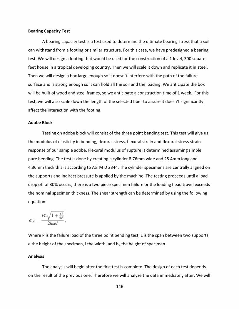
146

Bearing Capacity Test

A bearing capacity test is a test used to determine the ultimate bearing stress that a soil

can withstand from a footing or similar structure. For this case, we have predesigned a bearing

test. We will design a footing that would be used for the construction of a 1 level, 300 square

feet house in a tropical developing country. Then we will scale it down and replicate it in steel.

Then we will design a box large enough so it doesn’t interfere with the path of the failure

surface and is strong enough so it can hold all the soil and the loading. We anticipate the box

will be built of wood and steel frames, so we anticipate a construction time of 1 week. For this

test, we will also scale down the length of the selected fiber to assure it doesn’t significantly

affect the interaction with the footing.

Adobe Block

Testing on adobe block will consist of the three point bending test. This test will give us

the modulus of elasticity in bending, flexural stress, flexural strain and flexural stress strain

response of our sample adobe. Flexural modulus of rupture is determined assuming simple

pure bending. The test is done by creating a cylinder 8.76mm wide and 25.4mm long and

4.36mm thick this is according to ASTM D 2344. The cylinder specimens are centrally aligned on

the supports and indirect pressure is applied by the machine. The testing proceeds until a load

drop off of 30% occurs, there is a two piece specimen failure or the loading head travel exceeds

the nominal specimen thickness. The shear strength can be determined by using the following

equation:

Where P is the failure load of the three point bending test, L is the span between two supports,

e the height of the specimen, l the width, and h₀ the height of specimen.

Analysis

The analysis will begin after the first test is complete. The design of each test depends

on the result of the previous one. Therefore we will analyze the data immediately after. We will

147

run statistical analysis that validates the results by proving that the variation between different

groups of samples in the same test is significantly larger than the variation among specimens in

the same group. We aim to significantly improve the soil shear strength with the mixing of the

fibers. Whether or not there will be an increase and whether or not it will be significant, our

analysis will determine the real impact of its usage.