Soil Mechanics Prof. B.V.S. Viswanathan Department of...

Soil Mechanics Prof. B.V.S. Viswanathan

Department of Civil EngineeringIndian Institute of Technology, Bombay

Lecture – 50 Earth pressure Theories -I

Friends welcome to earth pressure theories part I. Having studied the shear strength of soils, now we need to extend our knowledge in arriving at earth pressures particularly on the retaining structures. So in this lecture we will be introducing the lateral earth pressure concepts, why we are required to study and where these lateral earth pressures are applied. So coming to the introduction, the first rigorous analysis of the problem of earth pressures was published by coulomb in 1776.

(Refer Slide Time: 01:22 min)

The first rigorous analysis of the problem of lateral earth pressure was published by Coulomb in 1776. Coulomb s theories were subsequently studied and supported by Rankine in 1857. Further it was studied and verilated by Terzaghi in 1934. These lateral pressures mainly for structures like anchor bulkheads, retaining walls and other structures that resist earth movement are in use since pre -Roman times. So the necessity, the pre Roman times this retaining walls has been constructed. So because of this in 1776 itself Coulomb has concentrated in evaluating and understanding the lateral earth pressure behavior and when the walls are subjected to these pressures and it has been studied and established. So in 1857 Rankine, verdicted the Coulombs theories and further work has been produced.

So particularly in the earth pressure theories we will be first studying Rankine earth pressure then we will be extending it to Coulomb earth pressure theories and then different graphical methods for computing lateral earth pressures on the walls. So this leads to the determination of lateral earth pressures coming when the retaining structures are subjected to movement. So the amount of lateral earth pressures depending upon whether wall is having movement or no movement or whether if it is having movement, if it is away from the field or towards the field.


So lateral forces most typically develop against structures from the presence of soil or water against vertical sections. So these lateral forces are basically developed against vertical sections, they are basically due to present soil or water alone or water along with the soil.


Retaining walls and foundation walls are representatives of structures to support an adjacent mass of the earth while dams are used to retain bodies of water. So large bodies of water retained by earth dams or dams. So you need to calculate this pressure exerted by the bodies of water on the earthen dam sections and all, so this knowledge on the lateral earth pressures is required. So retaining walls and foundation walls are basically for the basement walls of the multistoried buildings are representative of the structures to support an adjacent mass of the earth because when you consider, when we study in shear strength we understood that one angle called angle of repose. That is the maximum angle at which the soil can withstand without any support.

So that means many time situations arise that you need to maintain a vertical support that means that you have to retain the soil to prevent it again from the reaching that angle of repose. Anything angle which is steeper than the angle of repose the soil tends to settle to that angle. So if you want a steeper support, a steeper section then you need to support this particular soil against by using sections like retaining walls or basement walls in the form of foundation walls. So where do you come across this thing.


For example you have got a building and the basement wall and which is located and suppose if the building is having a drain and water is entering the drain. So in the process what happens is that you got a possibility of the accumulation of the water. If there is inadequate drainage or if the soil is not able to drain the water rapidly then what happens is that there is an accumulation of the water surrounding the basement wall. So this results in a pressure like which is highlighted here, it shows and then causes a destructs to the wall. So the one which is resulted because of the soil as well as the water which is exerted and that causes lateral earth pressure under the soil, on to the wall section.


So why to know about this means the reason is actually depicted schematically here from academic point of view where the water drain which is shown here and where the accumulation of the water and it results in the settling back fill and where the water pressure exerted on the wall. So it results in the distress in the basement wall section resulting due to the additional pressure which was not design for. So in view of the above it causes damage and the hasstic look of the basement or any interiors can get spoiled and then can endanger the safety of the building. In geotechnical engineering it is often necessary to prevent soil movements like we say if you have got a material which is settling at angle of repose, we can afford always to have materials with slopes with angle of repose.


Many times you are required to retain the soil to meet the public demand or utilities. So in such situations we need to resort for some structure like a cantilever retaining wall which is shown here, a wall section and then a surrounding soil. So here this particular soil is supported by laterally by a wall section which is there. So in order to design this particular wall section against failure, against design point of view you are require to know the lateral force exerted per meter length of the wall. So most of these structures which are particularly this cantilever retaining wall all this structures they are cone plane structures because they are basically the other directions, they have per meter length section which remains there. So the activity which remains in x and y directions, if x happens to be along this directions and y in this direction and they are perpendicular to the z direction is supposed to be. So in this particular type of structures, the long structures they are called plane strains structures. So here in the second diagram where it is shown a braced excavation. You can do the excavation without any support up to certain depth beyond that you are required to support with shutters and then these have to be braced with tie rods. So what you see here this particular section is again shows a typical braced excavations where the earth pressures have to be resisted by this shutter and then this is again force is transferred by this tie rods as compression members. What you see is anchored sheet pile walls where you have got a earth which is retained by a flexible structure

called a steel section and that is anchored by a anchor which is at a certain location. So the location of the anchor and the forces which are coming on the anchor and then the forces which are coming on the sheet file wall, all these things in order to design this particular type of structures in geotechnical engineering, it is often necessary to prevent soil movement and also in addition to that in order to retain this things we need to understand this lateral earth pressures which can be generated because of the complicated conditions in combination with different loadings which can exists.


So further a simple structure which are shown. We need to estimate lateral earth pressure acting on this structures and to be able to design them. So in the previous slide and then this slide the structures which are shown, we need to estimate the lateral earth pressure and then we need to design them. So in order to do that we need to understand about the theories behind this particular topic. So that’s what we are for and we are applying our knowledge of shear strength to this to understand about this particular lateral earth pressure theories. So here what you see a typical gravity retaining wall, so all its retaining capacity is derived from its own self weight and here you see a fill. In this case any soil which is behind that wall and which is referred here in as back fill, the wall or the fill material which is behind the wall referred here in as back fill material. So here what you see that a geotextile reinforced slope and reinforced soil wall because in the urban areas and because of the positive of the availability of the land scarcity of the land. These structures are becoming quite common and meeting the demands economically as well as you know in a rapid savings in the cost of the project and all. So the geotextile reinforced slopes and reinforced soil wall have got a particular prominence in designing the lateral earth pressure, extension of these and able to design them economically so that they can support this pressures which are exerted by the moving soil mass. So in this slide what we are intended to learn is the

typical retaining structures which can be possible like the one which is shown is a plane form where you can have a wall with vertical face and a foundation for this and a battered back.


So the wall face can be battered this side, so a battered back or a battered face and a stepped face. So you have got a plane face here and then a stepped face towards expose side and a stepped back. So these are the different types of retaining structures otherwise you have got L shaped retaining wall or T shaped retaining wall so this is referred as a cantilever retaining wall or in order to have more sliding resistance sometimes it is required at the base to position of shear key. So this is L shaped returning wall with extension for shear key to have adequate factor of safety again sliding and this is a buttressed. So the particular wall section is buttressed to a certain interval on the exterior side and the counter fort that is which is inside the field. So in this slide what we had seen is that a typical retaining structure. They can be in a plane form and their face can be battered back or battered face, stepped face or stepped back. Mostly these are quiet common battered back and battered face and then this T shaped retaining walls or some time with shear key and sometime when we wanted to have adequate resistance against the lateral pressure it is hard to require buttressed. So that is actually buttressed and counterfort retaining walls.


In this slide some typical retaining structures which may come cross for the basement wall that is they constructed in open or sold excavation. That means you will be excavating for certain depth to construct the basement. So the material will be removed and these lateral forces are exerted onto this basement walls. So in this case it’s possible that these things can exert lateral forces and here embedded walls constructed prior to excavation. Here what you see a vertical cross section and then this supported popped here and here this vertical wall which is supported with anchors. Then here we have got different types of returning structures sometime you have got diaphragm walls of concrete diaphragm walls panel, a panel type excavations are done and they are constructed. Basically they are done for offshore structures and contiguous bore wall, this particular wall section is that you will be driving the piles as very closed spacing and then they are connected.

Here the secant board Pile (Refer Slide Time: 13:56 min) is that almost this piles are constructed without any gap and then covered. So this actually forms as a retaining structure. So here you have another bridge abetments, basically when you have got bridges constructing then you have got abetments which are coming, the soil area which are supported when the bridge is commencing and similarly the bridge at the commencement as well as the bridge at the end so required abetments.

So here again you have a T shaped bridge abetment where you have got a garudar (Refer Slide Time: 14:06 min) sitting here and then in case the soil is not having a bearing capacity then you have got a piled bridge abetment and in this case embedded cantilever where the section will be embedded within the soil and then which is supported and now that the recent trend is to adopt cost economic constructions or to have construction with reinforced earth technology were the reinforced earth abetments are becoming popular. They are gaining momentum because of their savings and cost economics and aesthetics look which can give from duai (Refer Slide Time: 14:39 min) from adopting this technology. Then other techniques which is coming is called Gabion wall technology where you have got the locally available material like stones or rounded aggregates which cannot be used for any construction can be adopted to use in this. Then form a Gabion walls that means a prefabricated meshes will come and then they will be filled with this

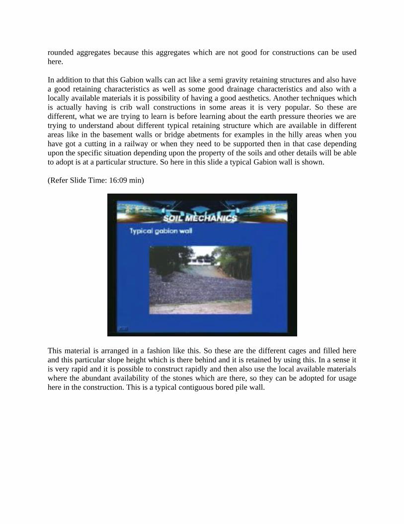
rounded aggregates because this aggregates which are not good for constructions can be used here. In addition to that this Gabion walls can act like a semi gravity retaining structures and also have a good retaining characteristics as well as some good drainage characteristics and also with a locally available materials it is possibility of having a good aesthetics. Another techniques which is actually having is crib wall constructions in some areas it is very popular. So these are different, what we are trying to learn is before learning about the earth pressure theories we are trying to understand about different typical retaining structure which are available in different areas like in the basement walls or bridge abetments for examples in the hilly areas when you have got a cutting in a railway or when they need to be supported then in that case depending upon the specific situation depending upon the property of the soils and other details will be able to adopt is at a particular structure. So here in this slide a typical Gabion wall is shown. (Refer Slide Time: 16:09 min)

This material is arranged in a fashion like this. So these are the different cages and filled here and this particular slope height which is there behind and it is retained by using this. In a sense it is very rapid and it is possible to construct rapidly and then also use the local available materials where the abundant availability of the stones which are there, so they can be adopted for usage here in the construction. This is a typical contiguous bored pile wall.


What you see is the typically bored walls bored piles have been driven and then they are attached to a beam. So what you can see is that a typical contiguous bored pile wall in this picture. So it is shown from the academic point of view for giving you an idea about how the contiguous bored pile wall look like.


Here for a basement of a building, you can see a soil or a surrounding area is protected by using another technique called soil nailing technique or this particular technique is generally used for temporary protection or sometimes for protection where in this case again the lateral earth pressure again countered by the nails which are embedded within the ground and they actually

take this lateral forces because of the soil nail interactions and the process the nail gets a tension which actually resist this lateral movement. So here what you see is that a facing and then this are the end connections for a nails and this is the basement which is coming up.


So these are the typical soil nail slope which is for a basement excavation otherwise if this slope is not supported so there is a danger of failure. (Refer Slide Time: 17:56 min)

So this is a typical crib wall which is shown here because this crib walls, they look like an open mesh type here and with headers and stretchers which are running like this. They have good

interlocking characteristics and what we need to do is that this entire fill material filled with soil here because this crib wall is having a good aesthetics that is one merit of this particular construction and good drainage and allow the plant growth. So where you have got environmental friendly aesthetic appearance which can mingle with surrounding environment very easily. So this is a typical crib wall where the possibility of interlock is created by this headers and stretchers which extended into the soil and then the soil will be filled in these gaps. So that they have the confinement which is actually required because of that it actually takes that lateral earth pressure which are exerted on to the wall. So before introducing let us look whether water can exert pressures or not. So a pool of water is shown here, a typical swimming pool.


So here the vertical stress and horizontal stress is same in the sense what will happen is that the sigmav or sigmah which is acting is same because the pressure is same in all directions. Another thing is that water is actually not having shear strength so because of that horizontal stress is equal to vertical stress. So the ratio sigmah by sigmav is equal to one for water. So if vertical column of water is there then it has got lateral pressure which is exerted and that is the stresses are equal in all directions. Why that is answered because it has no shear strength.

Contratrary to that if you look earth and water pressures let us consider that the T shaped retaining wall is retaining the water. So in this case here because of the concept which is introduced the total hydrostatic pressure is given by sigma is equal to sigmav equal to sigmah

because of the vertical direction and horizontal direction. Here the vertical directions pressure is also shown because sigmav is equal to sigmah because H is the height of the wall or the H is the height of the water which is retained with unit gammaw so with that what will happen is that sigmav is equal to sigmah is equal to gammaw H is the pressure at this particular point.


So the net force which is exerted on the wall if you look into it, so H is the height, gamma w H is the ordinate here so which is nothing but half gammaw H square is acting per meter length of this wall. Suppose if the length of the wall say 10 meters then the 10 meter length or this much total force is going to act laterally. Sometimes you consider this is a level which is indicated and then there is a soil which is gamma bulk having a moist soil and no water, in this case the vertical pressure sigmav is again indicated by gammab H where gammab is nothing but the bulk unit weight of soil and H is the height of this thing now that is because this stress is obtained. This is a vertical stress though it is a vertical stress it doesn’t indicate the direction of the stress.


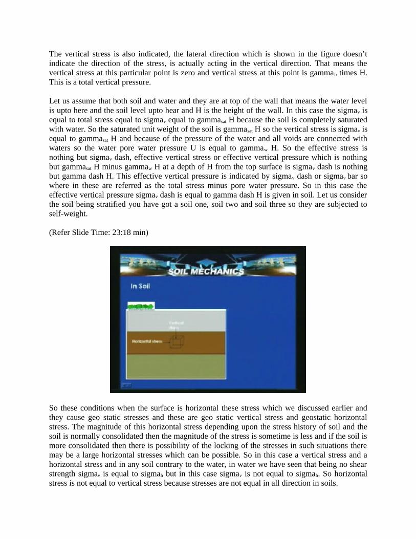
The vertical stress is also indicated, the lateral direction which is shown in the figure doesn’t indicate the direction of the stress, is actually acting in the vertical direction. That means the vertical stress at this particular point is zero and vertical stress at this point is gammab times H. This is a total vertical pressure.

Let us assume that both soil and water and they are at top of the wall that means the water level is upto here and the soil level upto hear and H is the height of the wall. In this case the sigmav is equal to total stress equal to sigmav equal to gammasat H because the soil is completely saturated with water. So the saturated unit weight of the soil is gammasat H so the vertical stress is sigmav is equal to gammasat H and because of the pressure of the water and all voids are connected with waters so the water pore water pressure U is equal to gammaw H. So the effective stress is nothing but sigmav dash, effective vertical stress or effective vertical pressure which is nothing but gammasat H minus gammaw H at a depth of H from the top surface is sigmav dash is nothing but gamma dash H. This effective vertical pressure is indicated by sigmav dash or sigmav bar so where in these are referred as the total stress minus pore water pressure. So in this case the effective vertical pressure sigmav dash is equal to gamma dash H is given in soil. Let us consider the soil being stratified you have got a soil one, soil two and soil three so they are subjected to self-weight.


So these conditions when the surface is horizontal these stress which we discussed earlier and they cause geo static stresses and these are geo static vertical stress and geostatic horizontal stress. The magnitude of this horizontal stress depending upon the stress history of soil and the soil is normally consolidated then the magnitude of the stress is sometime is less and if the soil is more consolidated then there is possibility of the locking of the stresses in such situations there may be a large horizontal stresses which can be possible. So in this case a vertical stress and a horizontal stress and in any soil contrary to the water, in water we have seen that being no shear strength sigmav is equal to sigmah but in this case sigmav is not equal to sigmah. So horizontal stress is not equal to vertical stress because stresses are not equal in all direction in soils.

So previously in water we have seen that they are equal but in this case they are different. The reason is the soil possesses shear strength. So because of that what we have is that in soil you have got a different vertical stresses and horizontal stresses and apportioning this, what component of horizontal stress is that depends upon the several factors like the type of material, the type of deposition and the way the stress history which was lying at a particular area and that can dictate this combination. So this lateral earth pressure when we wanted to introduce, the effective lateral pressures are determined by transferring a portion of the effective vertical pressure.


So that is what has been discussed now effective lateral earth pressures are determined by transferring a portion of the effective vertical pressure. That means their effective lateral earth pressures are determined by transferring a portion of the effective vertical pressure. This amount of transfer that means this is found to be depending upon the type and unit weight and the strength of the soil behind the wall and the direction amount of the wall movement. So the type and unit weight and the strength of the soil and soil behind the wall and the direction and amount of the wall movement. The amount of transfer is expressed in terms of a coefficient called lateral earth pressure coefficient.

The amount of transfer is expressed in terms of a lateral earth pressure coefficient called K. So lateral earth pressure coefficient can only be applied to effective vertical pressure. As you just now seen that when you have got a water pressure then the lateral earth pressure coefficient K is equal to 1, whereas in case of soil because of its shear strength characteristics, the possessing shear strength characteristics the lateral earth pressure is not equal to lateral earth pressure in the vertical direction. So lateral earth pressure is not equal to the vertical pressure, so the amount of transfer is expressed in terms of a lateral earth pressure coefficient K where K is equal to sigmah

dash by sigmav dash where sigmah dash is the effective horizontal pressure, sigmav dash is the effective vertical pressure and many notations are there k, k0. Even in this lecture also you see k, k0 or K areas, the notations but it is nothing but a lateral earth pressure coefficient at rest it is

called. So lateral earth pressure coefficient can only be applied to effective vertical pressure because the water cannot have this particular pressure so that K coefficient earth pressure at rest for coefficient of lateral earth pressure coefficient is equal to one for a case when the water is exerting a lateral pressure. So they cannot be applied to total pressures because the total pressure has the component of effective stress and component of water pressure. So when you have this component of water pressure is acting that means you cannot actually apply a coefficient lateral pressure coefficient to the water. So this lateral earth pressure coefficients can only be applied to, this always a misunderstood concept which students have to be noted that lateral earth pressure coefficient can only be applied to effective vertical pressures.

So let us consider a case where you have got, the previous case we considered a T shaped returning wall and a cantilever retaining wall is having a backfill which is saturated and it is having water level upto the brim of the wall that is at the top surface of the ground (Refer Slide Time: 27:49 min). So in this case the horizontal effective earth pressure is nothing but sigmah

dash is equal to K times gamma dash h. Here because gamma sat – gammaw that is the water pressure has been taken out. So what you have is that sigmah dash, horizontal effective pressure is equal to K time’s gamma dash h because this gamma dash h is the vertical stress component. Now what we have done is that by using k is equal to sigmah by sigmav or sigmah dash by sigmav

dash, so what we have try to find out is that K times gamma dash h is nothing but the lateral component.


So sigma h dash is equal to K gamma dash H and the pore water pressure is equal to u gammaw

H. So in case if you wanted to express that in the total lateral earth pressure then it has to be calculated as sigmah dash is equal to K gamma dash H plus gammaw H. So K gamma dash H plus gamma dash so if you note here the gammaw H though it’s in the lateral earth pressure which is acting but it doesn’t carry any coefficient. So here in case of total pressure what we have is that sigmah dash is equal to K gamma dash H.

So the lateral earth pressure coefficient is only applied to the effective horizontal stress which is here in this case, the effective pressure stress that is gamma dash H into K plus gammaw H. This is a deliberation what we discussed for lateral pressure in saturated backfill. There are many areas those theories which have been postulated. The Rankine first assumed that a wall or in a vertical section is assumed to be uniformly non yielding type that means a vertical section is assumed to remain in position, non-yielding type in the sense that there is no strain at all in the direction, no movement at all that is one case. Then there may be possibility that entire wall section moves away from the back fill parallel. So that is one type of possibility and another type of possibility is that one type of wall section can move towards the back fill.

So the categories of lateral earth pressure have been quantified like in case, if you have got normally consolidated clay and which is no longer undergoing any consolidation, in such situations there may not be any lateral earth pressure that means they may be non-yielding type. In such situation the coefficient of lateral earth pressure conditions like non yielding type can apply but if there are cases that where the chances of movement of the vertical section away from the back fill or towards the back fill then apportioning of that actually depends upon the particular theories. So these where actually first postulated by coulomb and then it was refined by Rankine. So in the Rankine’s theory we will be discussing about the Rankine theory and assumptions in the next lecture but here before that we will be understanding more about the non yielding type and we will try to correct which is required from the shear strength point of view. (Refer Slide Time: 31:18 min)

So here in this case many times the parallel sections which are the entire movement of the wall may not be possible. So in this case a typical T shaped retaining wall or a cantilever retaining wall was selected and this particular section which shows at rest case where no movement situation and in this case which is postulated and named by Rankine as active case where the wall tips or moves away from the soil. So when the wall actually moves away from the soil and this condition is called active case and the pressure or the lateral earth pressure which is computed in that case is actually called as active earth pressure.


If there is a case that the wall moves into the soil like it can happen in a situation like in bridge abetments where the wall can move into the soil. So there is actually possibility of passive case or if you have got a retaining wall and there is a fill which is in front and when the wall is actually moving away from the back fill, at the bottom portion or downstream portion the soil in front of it can be subjected to passive case because in bottom portion the soil will be moving towards the fill. For example at that point that actually becomes like a back fill and exerts a compressive forces into the soil.


So here what happens is that if these three cases which are states which are mentioned here called active case, at rest case and passive case. So mostly in at rest case where that no movement condition or zero strain condition which is called and that particular condition and then particular earth pressure, coefficient determined at the condition a zero strain condition is called coefficient of earth pressure at rest, that is called geo strain condition. So the soil strength and states of stress in a soil mass during the wall movement. So consider an isolated element in a backfill without any movement or strains in a soil mass.


So let us assume that you have got a cross section of a retaining wall, so figure above shows an element with the principle effective stresses acting on it. So here what you see is a vertical cross section of the wall, H is the height and this is the backfill with gammam is gamma moist is the backfill unit weight and this is the element under consideration, sigmav dash is the vertical principle stress because its called principle stress because no movement condition, those no shears stress, so the shear less planes are called principle planes. This is the horizontal plane and this is one principle plane where the shear is zero so sigmav dash. So this is the major principle stress and sigmav dash which is vertical principle stress acting on the horizontal plane and it’s the vertical plane is again a shear less plane then sigmah dash is the horizontal effective pressure.

So sigmah dash is equal to K sigmav where K is the lateral earth pressure coefficient, K is equal to k0 which is written here so sigmah dash is the effective horizontal pressure and K is the lateral earth pressure coefficient, sigmav is the lateral earth pressure, sigmav is the effective vertical pressure. So this particular figure shows a cross section element which is subjected to vertical effective pressures and horizontal effective pressure, the sigmah dash is equal to K times sigmav.


If the wall is allowed to deflect away from the backfill and develop some strain. In this slide what we have shown is that if the wall is allowed to move like this which is shown typically and deflect away from the backfill and develop some strain in the soil mass, the element undergoes some strain. So that is actually represented systematically in triaxial test we call. In the triaxial test this major principle stresses are simulated, vertical principle stress and horizontal principle stresses simulated in a similar way and by holding the horizontal principle stress this sigmah dash and increasing the sigmav dash the failure is induced the way it is shown here. So here alpha is the failure plane which is shown here, the possible failure plane and with a deflection because of the lateral strength in the direction develops.

So here what happens is that the sigmah dash which is the horizontal effective stress, sigmav dash is the vertical effective stress. So this towalpha is the shear stress along this plane and then the sigmaalpha is the normal stress which is acting here. So shear stress towalpha and normal stress sigmaalpha which act on potentially developing shear plane at an angle alpha from the. So this is a potential failure plane which is shown here. This shear plane development behind the wall yielding away from the backfill is shown. So when the wall yields backfill there is a possibility of a shear plane development. Here if the wall is allowed to deflect away from the backfill and develops some strain in the soil mass, the element also undergoes some strain.

So here what is been shown is that along this failure plane, this stresses are simulated. So these conditions are simulated experimentally to arrive at this strength properties towalpha and that stress condition along that failure plane that is at failure. If they reached to the failure then they tend to give the failure and we able to determine the properties. So let us look into this soil shear strength and state of stress in a soil mass during the wall movement. So here in this slide what we have taken is a particular element and then when it is subjected to the stress conditions, when it subjected to a movement away from the backfill.


So these conditions can be simulated in a triaxial or a direct shear test where the strain is induced which may be shear strain in case of a direct shear box or it can be by holding a constant sigmah

you can increase the vertical stress. So that is nothing but a deviator stress in case of a triaxial test. So moment it reaches the towf, it can reach to the failure. So these as gradually when it actually strain, there is a possibility of reaching towf then a failure of specimen can take place. So this actually shown a typical stress strain relationship here and this element which was shown in the previous slide is shown here is exaggerated and shown. This epsilon which is actually nothing but delta hs by hs that is the vertical strain, so here these conditions are simulated by applying the vertical deviatoric stress, so this failure conditions are simulated.

So K is equal to sigmah dash by sigmav dash or sigmah bar by sigmav bar when alpha is equal to 45 plus phi bar by 2. So these details you would have already acquainted yourself while looking into the shear strength aspects of soil. So here like this you do the number of samples like with different horizontal stresses then we get the different Mohr circles. This particular component which is called Mohr’s circle where we represent these conditions in a Mohr circle formation. So you can see here, this is for another combination of stresses, so you have got a sigma h1 then the responses here sigma h2 and sigma h3.

If you are able to join all this Mohr circle then you will get the envelop and that envelop is called the shear strength envelop and here this is the equation of this envelop lies like towalpha is equal sigmaalpha tan phi plus c bar. So c bar is that intercept here and that is called cohesion and this inclination of this shear strength envelope is called angle of internal friction. This c bar and phi bar and if they happened to be under consolidated drained condition or if you are referring as drained parameters they are called c dash or phi dash that is the drained parameters or the drained strength parameters of the soil. So in case if the pore pressure drainage is not allowed and for example in case of consolidated undrained conditions also, in case say unconsolidated undrained test you will get the undrained conditions.


So here whatever the element we have seen and if it is a granular soil and if it is a normally consolidated soil then the shear strength envelope which runs like this where c is equal to zero, in such situations the envelope lies there and if this conditions like if it this circle which is not touching this particular envelope that means it not yet reached the failure. In this case here this towalpha, sigmaalpha they are the shear stress conditions which are available here towalpha and sigmaalpha and which are actually less than shear stress which is actually failure stress, so in that case the failure is actually not attained. The moment it touches this failure envelope that means we can say that the failure is attained to the soil. So the Mohr stress conditions shown on the Mohr strength diagram where here is the shear strength envelops.


So as far as these things are concerned, the sample is said to be stable. The stress circle is not yet strength circle since the towalpha has not yet reached the maximum value before failure. So the towalpha not yet reached the maximum before failure. So here what you can see is that the stress circle which is represented, so this circle will become the Mohr strength circle, moment it becomes tangential to this envelope. This is actually when you do not have this analog in order to construct that you need to have test this sample at different horizontal pressures and create number of Mohr’s strength circles and by drawing a tangential line to this Mohr’s circles. Mohr strength circle will be able to generate an envelope and that envelope is actually resulting as the shear strength envelope. Here if you know the properties of a soil and here in this case a phi dash which is c dash is equal to zero and phi dash and in this case where we can say that the stress circle is not yet a strength circle sense that towalpha is not yet reached maximum value before failure.


So returning wall movement and related state of stress if you look in to it where we actually discussing about the k0 state where that is at rest condition, where the no movement arises and when the minimum that is deflection away from the backfill can create and the pressure will be minimum that is KA is called active earth pressure conditions when it actually moves away from the fill and then when the wall move towards fill that is deflection towards the backfill then there is a Kp which is actually maximum. So the coefficient Ka is minimum when it is actually moving away from the backfill and Kp is maximum when it is actually moving towards the backfill. So apportioning of that will be depending upon the surrounding soils properties and other conditions which will be discussing.

The possible wall deflection and related range of lateral earth pressure coefficient are shown here where you have got that is at rest condition or no yielding conditions or zero strain conditions is called k0 condition, is called coefficient of earth pressure at rest condition. So non yielding walls at rest conditions let us consider, the non-yielding conditions at rest condition. At rest condition

is defined a state of zero of lateral yielding and there is no lateral strength that is epsilon is equal to zero.


At rest condition is defined as a state of zero lateral yielding and there is no lateral strength that means you have got a typical cantilever wall and you have got sigmav dash and sigmah dash where epsilon is equal to zero, so K0 is equal to sigmah dash by sigmav dash. So here sigmah dash is the horizontal effective stress at rest condition that is because of the K times or K0 times the vertical effective stress.

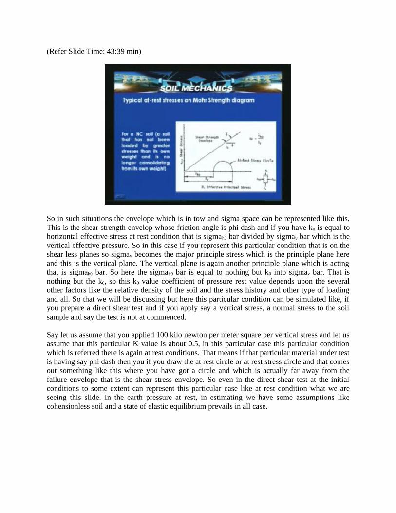
Where in this case the epsilon is equal to zero that is actually the wall is at rest backfill that is non-yielding type. So if this typical at rest stresses on motion diagram if you represent for a normally consolidated soil means that a soil that has not been loaded by greater stresses than its own weight and is no longer consolidating from its own weight. That means a normally consolidated soil or the soil that has not been loaded by greater stresses than its own weight and is no longer consolidating from its own weight.


So in such situations the envelope which is in tow and sigma space can be represented like this. This is the shear strength envelop whose friction angle is phi dash and if you have k0 is equal to horizontal effective stress at rest condition that is sigmah0 bar divided by sigmav bar which is the vertical effective pressure. So in this case if you represent this particular condition that is on the shear less planes so sigmav becomes the major principle stress which is the principle plane here and this is the vertical plane. The vertical plane is again another principle plane which is acting that is sigmah0 bar. So here the sigmah0 bar is equal to nothing but k0 into sigmav bar. That is nothing but the k0, so this k0 value coefficient of pressure rest value depends upon the several other factors like the relative density of the soil and the stress history and other type of loading and all. So that we will be discussing but here this particular condition can be simulated like, if you prepare a direct shear test and if you apply say a vertical stress, a normal stress to the soil sample and say the test is not at commenced.

Say let us assume that you applied 100 kilo newton per meter square per vertical stress and let us assume that this particular K value is about 0.5, in this particular case this particular condition which is referred there is again at rest conditions. That means if that particular material under test is having say phi dash then you if you draw the at rest circle or at rest stress circle and that comes out something like this where you have got a circle and which is actually far away from the failure envelope that is the shear stress envelope. So even in the direct shear test at the initial conditions to some extent can represent this particular case like at rest condition what we are seeing this slide. In the earth pressure at rest, in estimating we have some assumptions like cohensionless soil and a state of elastic equilibrium prevails in all case.


That means we assume that the elastic equilibrium conditions and no external loading stresses are only due to gravity that means only geostatic conditions and no lateral strains that means the lateral strengths are zero no permanent deformation in the lateral directions. Importantly at k0

state there are no lateral stresses so the important thing is that at k0 state there are no lateral stresses.


So coefficient of earth pressure at rest can be determined at a particular depth. Say if this happens to be like sigmav dash and sigmah dash and if this at a particular depth z at a point which is shown there then coefficient of earth pressure k0 is equal to sigmah by sigmav. So soil deforms

under its own self weight but it is prevented from deforming laterally because of its infinite extent in lateral directions. So at particular point this dot if you take, the soil deforms under its own weight but it is prevented from deforming laterally because of its infinite extent in all directions. So using the theory of elasticity fundamentals, if you write the lateral strain epsilon is equal to sigmah by e assuming that cooks law is valid sigmah by E where is modulus of the elasticity of the material soil.


That is minus mu into sigmav by E plus sigmah by E is equal to zero where mu is the Poisson’s ratio and sigmav is the vertical stress and sigmah is the horizontal stress. So by simplifying this because the lateral strain is zero in k0 state, the wall is non-yielding type then sigmah by sigmav

by simplifying this, it results like sigmah by sigmav is equal to mu by 1- mu. So sigmah by sigmav

is related with Poisson’s ration which is mu by 1-mu. In a normally consolidated soil deposit the vertical principle stress is equal to the overburden. So that means in a normally consolidated soil deposit the over consolidation ratio will be equal to one. So with that we can write sigmav is equal to gamma z.


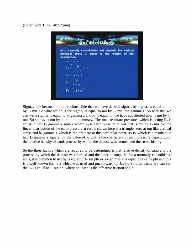
Sigmah now because in the previous slide that we have derived sigmah by sigmav is equal to mu by 1- mu. So what we do is the sigmah is equal to mu by 1- mu into gamma z. So with that we can write sigmah is equal to k0 gamma z and k0 is equal to, we have substituted now is mu by 1-mu. So sigmah is mu by 1- mu into gamma z. The total resultant pressures which is acting P 0 is equal to half k0 gamma z square where k0 is earth pressure at rest that is mu by 1- mu. So the linear distribution of the earth pressure at rest is shown here is a triangle, zero at top like vertical stress and k0 gamma z which is the ordinate at this particular point, so P0 which is a resultant is half k0 gamma z square. So the value of k0 that is the coefficient of earth pressure depend upon the relative density of sand, process by which the deposit was formed and the stress history.

So the three factors which are required to be determined is that relative density of sand and the process by which the deposit was formed and the stress history. So for a normally consolidated soils, it is common to use k0 is equal to 1- sin phi or sometimes k is equal to 1- sine phi and this is a well-known formula which was used and put forward by Jacky. So after Jacky we can say that k0 is equal to 1- sin phi where phi dash is the effective friction angle.


For over consolidated clays like k0 is equal to 1- sin phi dash into OCR to the raise power sin phi dash. Sometimes the deliberations like many empirical pressure like k0 is equal to 1- sine phi dash OCR to power of 0.5 is also in use. For over consolidated clays k0 is equal 1- sine phi dash OCR where OCR is the overconsolidated ratio and sine phi dash raised to the power of sin phi dash is also in use, the k0 is often normally consolidated clays is related to the plasticity index also.


And this was after Alpha 1967 where k0 is equal to 0.19 plus 0.233 log to the base PI. So with an increase in the plasticity index you can see that there will be a change in the value of the

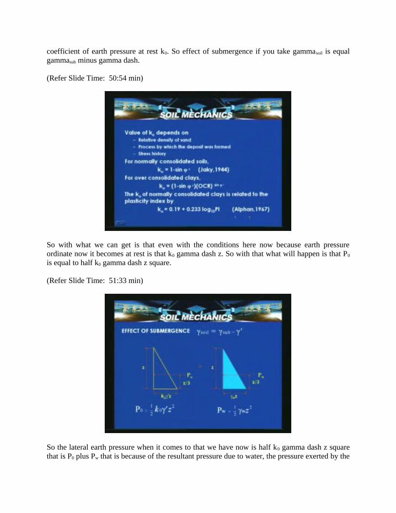
coefficient of earth pressure at rest k0. So effect of submergence if you take gammasoil is equal gammasub minus gamma dash.


So with what we can get is that even with the conditions here now because earth pressure ordinate now it becomes at rest is that k0 gamma dash z. So with that what will happen is that P0

is equal to half k0 gamma dash z square.


So the lateral earth pressure when it comes to that we have now is half k0 gamma dash z square that is P0 plus Pw that is because of the resultant pressure due to water, the pressure exerted by the

water. When you are actually dealing about this particular half k0 gamma dash z square plus half gammaw z square.


So in the next lecture that is under earth pressure theories two, what we do is that we will introduce to the Rankine’s earth pressure theory and then different cases which are actually governed under this particular theory will be discussed and we will try to look into some problems and obligations of that Rankine’s theories and assumptions which are involved in that and then which are connected to again by adopting the Mohr’s circles and this in a tow sigma space, how this active conditions and passive conditions can be simulated for a given material. It can be cohensionless soil, cohesive soil can be discussed. So in the next class we will be discussing about this Rankine’s earth pressures theory. So this lecture what we try to look into it is that we introduce the earth pressures theories and then the relevance for determination of earth pressure, need for understanding the earth pressures and discussed length about the earth pressure at rest and where the non yielding case may be certain situations like we have got a normally consolidated soil has a backfill deposit and where it’s the case where which not really exist and in that situations this is possible for us to have at rest conditions but the majority of conditions where we have is that active conditions where you tend to design for active state. So that will be discussing it in the next lecture.

Soil Mechanics Prof. B.V.S. Viswanathan Department of...

Documents

Transcript of Soil Mechanics Prof. B.V.S. Viswanathan Department of...