Software Quality Metrics Overview - Pearson · Software quality metrics are a subset of software...
42
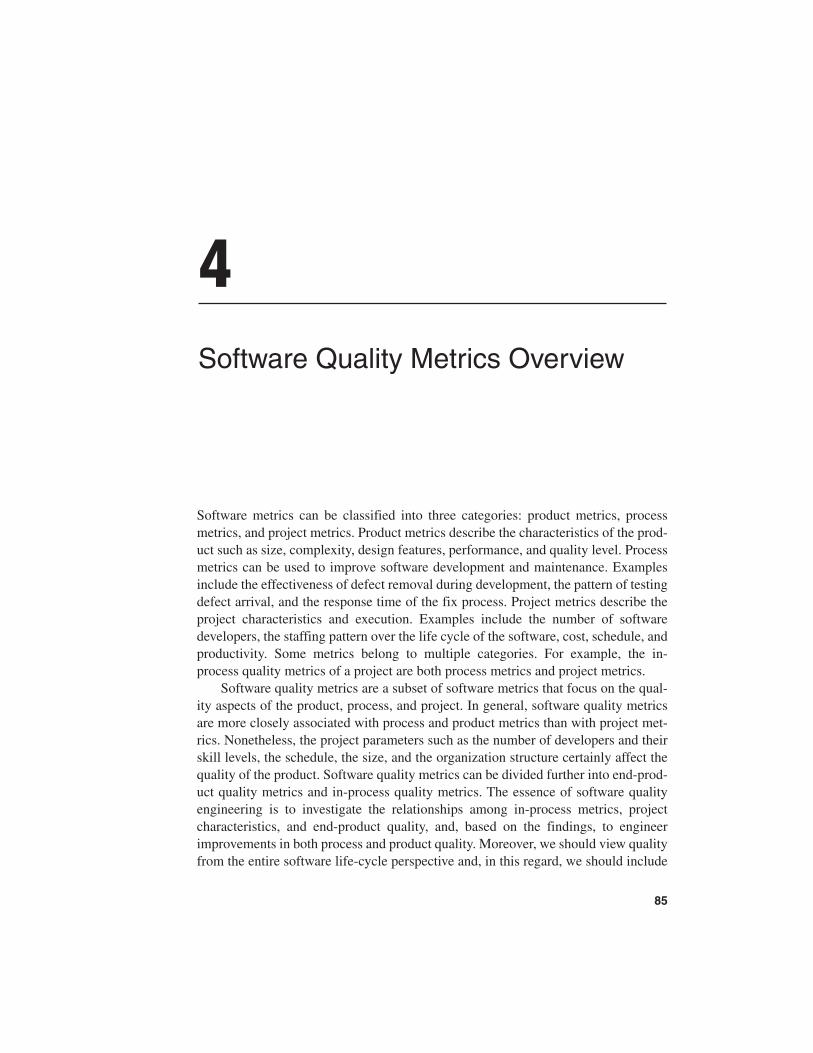
4 Software Quality Metrics Overview Software metrics can be classified into three categories: product metrics, process metrics, and project metrics. Product metrics describe the characteristics of the prod- uct such as size, complexity, design features, performance, and quality level. Process metrics can be used to improve software development and maintenance. Examples include the effectiveness of defect removal during development, the pattern of testing defect arrival, and the response time of the fix process. Project metrics describe the project characteristics and execution. Examples include the number of software developers, the staffing pattern over the life cycle of the software, cost, schedule, and productivity. Some metrics belong to multiple categories. For example, the in- process quality metrics of a project are both process metrics and project metrics. Software quality metrics are a subset of software metrics that focus on the qual- ity aspects of the product, process, and project. In general, software quality metrics are more closely associated with process and product metrics than with project met- rics. Nonetheless, the project parameters such as the number of developers and their skill levels, the schedule, the size, and the organization structure certainly affect the quality of the product. Software quality metrics can be divided further into end-prod- uct quality metrics and in-process quality metrics. The essence of software quality engineering is to investigate the relationships among in-process metrics, project characteristics, and end-product quality, and, based on the findings, to engineer improvements in both process and product quality. Moreover, we should view quality from the entire software life-cycle perspective and, in this regard, we should include 85
Transcript of Software Quality Metrics Overview - Pearson · Software quality metrics are a subset of software...
4Software Quality Metrics Overview
Software metrics can be classified into three categories: product metrics, processmetrics, and project metrics. Product metrics describe the characteristics of the prod-uct such as size, complexity, design features, performance, and quality level. Processmetrics can be used to improve software development and maintenance. Examplesinclude the effectiveness of defect removal during development, the pattern of testingdefect arrival, and the response time of the fix process. Project metrics describe theproject characteristics and execution. Examples include the number of softwaredevelopers, the staffing pattern over the life cycle of the software, cost, schedule, andproductivity. Some metrics belong to multiple categories. For example, the in-process quality metrics of a project are both process metrics and project metrics.
Software quality metrics are a subset of software metrics that focus on the qual-ity aspects of the product, process, and project. In general, software quality metricsare more closely associated with process and product metrics than with project met-rics. Nonetheless, the project parameters such as the number of developers and theirskill levels, the schedule, the size, and the organization structure certainly affect thequality of the product. Software quality metrics can be divided further into end-prod-uct quality metrics and in-process quality metrics. The essence of software qualityengineering is to investigate the relationships among in-process metrics, projectcharacteristics, and end-product quality, and, based on the findings, to engineerimprovements in both process and product quality. Moreover, we should view qualityfrom the entire software life-cycle perspective and, in this regard, we should include
85
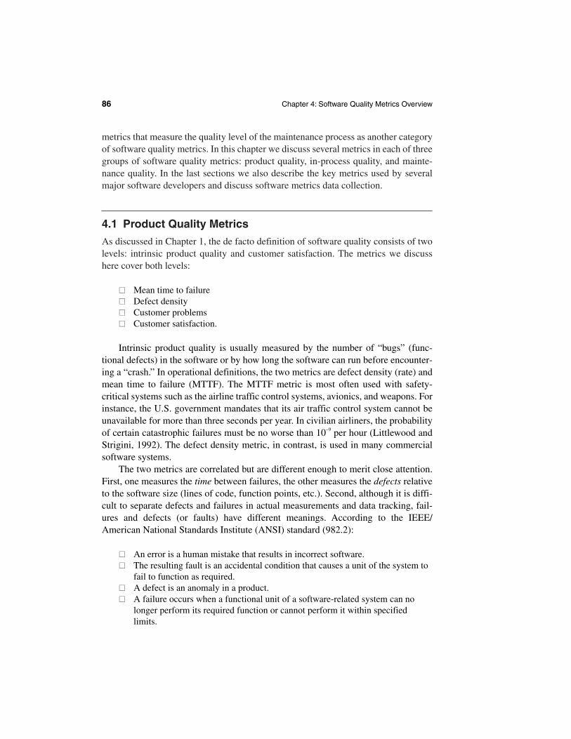
metrics that measure the quality level of the maintenance process as another categoryof software quality metrics. In this chapter we discuss several metrics in each of threegroups of software quality metrics: product quality, in-process quality, and mainte-nance quality. In the last sections we also describe the key metrics used by severalmajor software developers and discuss software metrics data collection.
4.1 Product Quality Metrics
As discussed in Chapter 1, the de facto definition of software quality consists of twolevels: intrinsic product quality and customer satisfaction. The metrics we discusshere cover both levels:
�� Mean time to failure�� Defect density�� Customer problems�� Customer satisfaction.
Intrinsic product quality is usually measured by the number of “bugs” (func-tional defects) in the software or by how long the software can run before encounter-ing a “crash.” In operational definitions, the two metrics are defect density (rate) andmean time to failure (MTTF). The MTTF metric is most often used with safety-critical systems such as the airline traffic control systems, avionics, and weapons. Forinstance, the U.S. government mandates that its air traffic control system cannot beunavailable for more than three seconds per year. In civilian airliners, the probabilityof certain catastrophic failures must be no worse than 10−9 per hour (Littlewood andStrigini, 1992). The defect density metric, in contrast, is used in many commercialsoftware systems.
The two metrics are correlated but are different enough to merit close attention.First, one measures the time between failures, the other measures the defects relativeto the software size (lines of code, function points, etc.). Second, although it is diffi-cult to separate defects and failures in actual measurements and data tracking, fail-ures and defects (or faults) have different meanings. According to the IEEE/American National Standards Institute (ANSI) standard (982.2):
�� An error is a human mistake that results in incorrect software.�� The resulting fault is an accidental condition that causes a unit of the system to
fail to function as required.�� A defect is an anomaly in a product.�� A failure occurs when a functional unit of a software-related system can no
longer perform its required function or cannot perform it within specifiedlimits.
86 Chapter 4: Software Quality Metrics Overview
4.1 Product Quality Metrics 87
From these definitions, the difference between a fault and a defect is unclear. Forpractical purposes, there is no difference between the two terms. Indeed, in manydevelopment organizations the two terms are used synonymously. In this book wealso use the two terms interchangeably.
Simply put, when an error occurs during the development process, a fault or adefect is injected in the software. In operational mode, failures are caused by faults ordefects, or failures are materializations of faults. Sometimes a fault causes more thanone failure situation and, on the other hand, some faults do not materialize until thesoftware has been executed for a long time with some particular scenarios.Therefore, defect and failure do not have a one-to-one correspondence.
Third, the defects that cause higher failure rates are usually discovered andremoved early. The probability of failure associated with a latent defect is called itssize, or “bug size.” For special-purpose software systems such as the air traffic con-trol systems or the space shuttle control systems, the operations profile and scenariosare better defined and, therefore, the time to failure metric is appropriate. For gen-eral-purpose computer systems or commercial-use software, for which there is notypical user profile of the software, the MTTF metric is more difficult to implementand may not be representative of all customers.
Fourth, gathering data about time between failures is very expensive. It requiresrecording the occurrence time of each software failure. It is sometimes quite difficultto record the time for all the failures observed during testing or operation. To be use-ful, time between failures data also requires a high degree of accuracy. This is per-haps the reason the MTTF metric is not widely used by commercial developers.
Finally, the defect rate metric (or the volume of defects) has another appeal tocommercial software development organizations. The defect rate of a product or theexpected number of defects over a certain time period is important for cost andresource estimates of the maintenance phase of the software life cycle.
Regardless of their differences and similarities, MTTF and defect density are thetwo key metrics for intrinsic product quality. Accordingly, there are two main typesof software reliability growth models—the time between failures models and thedefect count (defect rate) models. We discuss the two types of models and provideseveral examples of each type in Chapter 8.
4.1.1 The Defect Density Metric
Although seemingly straightforward, comparing the defect rates of software prod-ucts involves many issues. In this section we try to articulate the major points. Todefine a rate, we first have to operationalize the numerator and the denominator, andspecify the time frame. As discussed in Chapter 3, the general concept of defect rateis the number of defects over the opportunities for error (OFE) during a specific timeframe. We have just discussed the definitions of software defect and failure. Because
failures are defects materialized, we can use the number of unique causes of ob-served failures to approximate the number of defects in the software. The denomina-tor is the size of the software, usually expressed in thousand lines of code (KLOC) orin the number of function points. In terms of time frames, various operational defin-itions are used for the life of product (LOP), ranging from one year to many yearsafter the software product’s release to the general market. In our experience withoperating systems, usually more than 95% of the defects are found within four yearsof the software’s release. For application software, most defects are normally foundwithin two years of its release.
Lines of Code
The lines of code (LOC) metric is anything but simple. The major problem comesfrom the ambiguity of the operational definition, the actual counting. In the earlydays of Assembler programming, in which one physical line was the same as oneinstruction, the LOC definition was clear. With the availability of high-level lan-guages the one-to-one correspondence broke down. Differences between physicallines and instruction statements (or logical lines of code) and differences among lan-guages contribute to the huge variations in counting LOCs. Even within the samelanguage, the methods and algorithms used by different counting tools can cause sig-nificant differences in the final counts. Jones (1986) describes several variations:
�� Count only executable lines.�� Count executable lines plus data definitions.�� Count executable lines, data definitions, and comments.�� Count executable lines, data definitions, comments, and job control language.�� Count lines as physical lines on an input screen.�� Count lines as terminated by logical delimiters.
To illustrate the variations in LOC count practices, let us look at a few examplesby authors of software metrics. In Boehm’s well-known book Software EngineeringEconomics (1981), the LOC counting method counts lines as physical lines andincludes executable lines, data definitions, and comments. In Software EngineeringMetrics and Models by Conte et al. (1986), LOC is defined as follows:
A line of code is any line of program text that is not a comment or blank line,regardless of the number of statements or fragments of statements on the line.This specifically includes all lines containing program headers, declarations,and executable and non-executable statements. (p. 35)
Thus their method is to count physical lines including prologues and data defin-itions (declarations) but not comments. In Programming Productivity by Jones
88 Chapter 4: Software Quality Metrics Overview
4.1 Product Quality Metrics 89
(1986), the source instruction (or logical lines of code) method is used. The methodused by IBM Rochester is also to count source instructions including executablelines and data definitions but excluding comments and program prologues.
The resultant differences in program size between counting physical lines andcounting instruction statements are difficult to assess. It is not even known whichmethod will result in a larger number. In some languages such as BASIC, PASCAL,and C, several instruction statements can be entered on one physical line. On theother hand, instruction statements and data declarations might span several physicallines, especially when the programming style aims for easy maintenance, which isnot necessarily done by the original code owner. Languages that have a fixed columnformat such as FORTRAN may have the physical-lines-to-source-instructions ratioclosest to one. According to Jones (1992), the difference between counts of physicallines and counts including instruction statements can be as large as 500%; and theaverage difference is about 200%, with logical statements outnumbering physicallines. In contrast, for COBOL the difference is about 200% in the opposite direction,with physical lines outnumbering instruction statements.
There are strengths and weaknesses of physical LOC and logical LOC (Jones,2000). In general, logical statements are a somewhat more rational choice for qualitydata. When any data on size of program products and their quality are presented, themethod for LOC counting should be described. At the minimum, in any publicationof quality when LOC data is involved, the author should state whether the LOCcounting method is based on physical LOC or logical LOC.
Furthermore, as discussed in Chapter 3, some companies may use the straightLOC count (whatever LOC counting method is used) as the denominator for calcu-lating defect rate, whereas others may use the normalized count (normalized toAssembler-equivalent LOC based on some conversion ratios) for the denominator.Therefore, industrywide standards should include the conversion ratios from high-level language to Assembler. So far, very little research on this topic has been pub-lished. The conversion ratios published by Jones (1986) are the most well known inthe industry. As more and more high-level languages become available for softwaredevelopment, more research will be needed in this area.
When straight LOC count data is used, size and defect rate comparisons acrosslanguages are often invalid. Extreme caution should be exercised when comparingthe defect rates of two products if the operational definitions (counting) of LOC,defects, and time frame are not identical. Indeed, we do not recommend such com-parisons. We recommend comparison against one’s own history for the sake ofmeasuring improvement over time.
Note: The LOC discussions in this section are in the context of defect rate calcu-lation. For productivity studies, the problems with using LOC are more severe. Abasic problem is that the amount of LOC in a softare program is negatively correlatedwith design efficiency. The purpose of software is to provide certain functionality for
solving some specific problems or to perform certain tasks. Efficient design providesthe functionality with lower implementation effort and fewer LOCs. Therefore, usingLOC data to measure software productivity is like using the weight of an airplane tomeasure its speed and capability. In addition to the level of languages issue, LOCdata do not reflect noncoding work such as the creation of requirements, specifica-tions, and user manuals. The LOC results are so misleading in productivity studiesthat Jones states “using lines of code for productivity studies involving multiple lan-guages and full life cycle activities should be viewed as professional malpractice”(2000, p. 72). For detailed discussions of LOC and function point metrics, seeJones’s work (1986, 1992, 1994, 1997, 2000).
When a software product is released to the market for the first time, and when acertain LOC count method is specified, it is relatively easy to state its quality level(projected or actual). For example, statements such as the following can be made:“This product has a total of 50 KLOC; the latent defect rate for this product duringthe next four years is 2.0 defects per KLOC.” However, when enhancements aremade and subsequent versions of the product are released, the situation becomesmore complicated. One needs to measure the quality of the entire product as well asthe portion of the product that is new. The latter is the measurement of true develop-ment quality—the defect rate of the new and changed code. Although the defect ratefor the entire product will improve from release to release due to aging, the defectrate of the new and changed code will not improve unless there is real improvementin the development process. To calculate defect rate for the new and changed code,the following must be available:
�� LOC count: The entire software product as well as the new and changed codeof the release must be available.
�� Defect tracking: Defects must be tracked to the release origin—the portion ofthe code that contains the defects and at what release the portion was added,changed, or enhanced. When calculating the defect rate of the entire product,all defects are used; when calculating the defect rate for the new and changedcode, only defects of the release origin of the new and changed code areincluded.
These tasks are enabled by the practice of change flagging. Specifically, when a newfunction is added or an enhancement is made to an existing function, the new andchanged lines of code are flagged with a specific identification (ID) number throughthe use of comments. The ID is linked to the requirements number, which is usuallydescribed briefly in the module’s prologue. Therefore, any changes in the programmodules can be linked to a certain requirement. This linkage procedure is part of thesoftware configuration management mechanism and is usually practiced by organi-zations that have an established process. If the change-flagging IDs and requirements
90 Chapter 4: Software Quality Metrics Overview
4.1 Product Quality Metrics 91
IDs are further linked to the release number of the product, the LOC counting toolscan use the linkages to count the new and changed code in new releases. The change-flagging practice is also important to the developers who deal with problem determi-nation and maintenance. When a defect is reported and the fault zone determined, thedeveloper can determine in which function or enhancement pertaining to whatrequirements at what release origin the defect was injected.
The new and changed LOC counts can also be obtained via the delta-librarymethod. By comparing program modules in the original library with the new ver-sions in the current release library, the LOC count tools can determine the amountof new and changed code for the new release. This method does not involve thechange-flagging method. However, change flagging remains very important formaintenance. In many software development environments, tools for automaticchange flagging are also available.
Example: Lines of Code Defect Rates
At IBM Rochester, lines of code data is based on instruction statements (logicalLOC) and includes executable code and data definitions but excludes comments.LOC counts are obtained for the total product and for the new and changed code ofthe new release. Because the LOC count is based on source instructions, the two sizemetrics are called shipped source instructions (SSI) and new and changed sourceinstructions (CSI), respectively. The relationship between the SSI count and the CSIcount can be expressed with the following formula:
SSI (current release) = SSI (previous release)+ CSI (new and changed code instructions for
current release)− deleted code (usually very small)− changed code (to avoid double count in both
SSI and CSI)
Defects after the release of the product are tracked. Defects can be field defects,which are found by customers, or internal defects, which are found internally. Theseveral postrelease defect rate metrics per thousand SSI (KSSI) or per thousand CSI(KCSI) are:
(1) Total defects per KSSI (a measure of code quality of the total product)
(2) Field defects per KSSI (a measure of defect rate in the field)
(3) Release-origin defects (field and internal) per KCSI (a measure of developmentquality)
(4) Release-origin field defects per KCSI (a measure of development quality perdefects found by customers)
Metric (1) measures the total release code quality, and metric (3) measures thequality of the new and changed code. For the initial release where the entire productis new, the two metrics are the same. Thereafter, metric (1) is affected by aging andthe improvement (or deterioration) of metric (3). Metrics (1) and (3) are processmeasures; their field counterparts, metrics (2) and (4) represent the customer’s per-spective. Given an estimated defect rate (KCSI or KSSI), software developers canminimize the impact to customers by finding and fixing the defects before customersencounter them.
Customer’s Perspective
The defect rate metrics measure code quality per unit. It is useful to drive qualityimprovement from the development team’s point of view. Good practice in softwarequality engineering, however, also needs to consider the customer’s perspective.Assume that we are to set the defect rate goal for release-to-release improvement ofone product. From the customer’s point of view, the defect rate is not as relevant asthe total number of defects that might affect their business. Therefore, a good defectrate target should lead to a release-to-release reduction in the total number of defects,regardless of size. If a new release is larger than its predecessors, it means the defectrate goal for the new and changed code has to be significantly better than that of theprevious release in order to reduce the total number of defects.
Consider the following hypothetical example:
Initial Release of Product Y
KCSI = KSSI = 50 KLOCDefects/KCSI = 2.0Total number of defects = 2.0 × 50 = 100
Second Release
KCSI = 20KSSI = 50 + 20 (new and changed lines of code) − 4 (assuming 20% are changed
lines of code ) = 66Defect/KCSI = 1.8 (assuming 10% improvement over the first release)Total number of additional defects = 1.8 × 20 = 36
Third Release
KCSI = 30KSSI = 66 + 30 (new and changed lines of code) − 6 (assuming the same % (20%)
of changed lines of code) = 90Targeted number of additional defects (no more than previous release) = 36Defect rate target for the new and changed lines of code: 36/30 = 1.2 defects/KCSIor lower
92 Chapter 4: Software Quality Metrics Overview
4.1 Product Quality Metrics 93
From the initial release to the second release the defect rate improved by 10%.However, customers experienced a 64% reduction [(100 − 36)/100] in the number ofdefects because the second release is smaller. The size factor works against the thirdrelease because it is much larger than the second release. Its defect rate has to be one-third (1.2/1.8) better than that of the second release for the number of new defects notto exceed that of the second release. Of course, sometimes the difference between thetwo defect rate targets is very large and the new defect rate target is deemed notachievable. In those situations, other actions should be planned to improve the qual-ity of the base code or to reduce the volume of postrelease field defects (i.e., by find-ing them internally).
Function Points
Counting lines of code is but one way to measure size. Another one is the functionpoint. Both are surrogate indicators of the opportunities for error (OFE) in the defectdensity metrics. In recent years the function point has been gaining acceptance inapplication development in terms of both productivity (e.g., function points perperson-year) and quality (e.g., defects per function point). In this section we providea concise summary of the subject.
A function can be defined as a collection of executable statements that performsa certain task, together with declarations of the formal parameters and local variablesmanipulated by those statements (Conte et al., 1986). The ultimate measure of soft-ware productivity is the number of functions a development team can produce givena certain amount of resource, regardless of the size of the software in lines of code.The defect rate metric, ideally, is indexed to the number of functions a software pro-vides. If defects per unit of functions is low, then the software should have betterquality even though the defects per KLOC value could be higher—when the func-tions were implemented by fewer lines of code. However, measuring functions istheoretically promising but realistically very difficult.
The function point metric, originated by Albrecht and his colleagues at IBM inthe mid-1970s, however, is something of a misnomer because the technique does notmeasure functions explicitly (Albrecht, 1979). It does address some of the problemsassociated with LOC counts in size and productivity measures, especially the differ-ences in LOC counts that result because different levels of languages are used. It is aweighted total of five major components that comprise an application:
�� Number of external inputs (e.g., transaction types) × 4�� Number of external outputs (e.g., report types) × 5�� Number of logical internal files (files as the user might conceive them, not
physical files) × 10�� Number of external interface files (files accessed by the application but not
maintained by it) × 7�� Number of external inquiries (types of online inquiries supported) × 4

These are the average weighting factors. There are also low and high weighting fac-tors, depending on the complexity assessment of the application in terms of the fivecomponents (Kemerer and Porter, 1992; Sprouls, 1990):
�� External input: low complexity, 3; high complexity, 6�� External output: low complexity, 4; high complexity, 7�� Logical internal file: low complexity, 7; high complexity, 15�� External interface file: low complexity, 5; high complexity, 10�� External inquiry: low complexity, 3; high complexity, 6
The complexity classification of each component is based on a set of standardsthat define complexity in terms of objective guidelines. For instance, for the externaloutput component, if the number of data element types is 20 or more and the numberof file types referenced is 2 or more, then complexity is high. If the number of dataelement types is 5 or fewer and the number of file types referenced is 2 or 3, thencomplexity is low.
With the weighting factors, the first step is to calculate the function counts (FCs)based on the following formula:
where wij
are the weighting factors of the five components by complexity level (low,average, high) and x
ijare the numbers of each component in the application.
The second step involves a scale from 0 to 5 to assess the impact of 14 generalsystem characteristics in terms of their likely effect on the application. The 14 char-acteristics are:
1. Data communications2. Distributed functions3. Performance4. Heavily used configuration5. Transaction rate6. Online data entry7. End-user efficiency8. Online update9. Complex processing
10. Reusability11. Installation ease12. Operational ease13. Multiple sites14. Facilitation of change
94 Chapter 4: Software Quality Metrics Overview
FC = ×= =
∑ ∑i
ij ijj
w x1
5
1
3
4.1 Product Quality Metrics 95
The scores (ranging from 0 to 5) for these characteristics are then summed, based onthe following formula, to arrive at the value adjustment factor (VAF)
where ci
is the score for general system characteristic i. Finally, the number offunction points is obtained by multiplying function counts and the value adjustmentfactor:
FP = FC × VAF
This equation is a simplified description of the calculation of function points. Oneshould consult the fully documented methods, such as the International FunctionPoint User’s Group Standard (IFPUG, 1999), for a complete treatment.
Over the years the function point metric has gained acceptance as a key produc-tivity measure in the application world. In 1986 the IFPUG was established. TheIFPUG counting practices committee is the de facto standards organization for func-tion point counting methods (Jones, 1992, 2000). Classes and seminars on functionpoints counting and applications are offered frequently by consulting firms and atsoftware conferences. In application contract work, the function point is often usedto measure the amount of work, and quality is expressed as defects per functionpoint. In systems and real-time software, however, the function point has been slowto gain acceptance. This is perhaps due to the incorrect impression that functionpoints work only for information systems (Jones, 2000), the inertia of the LOC-related practices, and the effort required for function points counting. Intriguingly,similar observations can be made about function point use in academic research.
There are also issues related to the function point metric. Fundamentally, themeaning of function point and the derivation algorithm and its rationale may needmore research and more theoretical groundwork. There are also many variations incounting function points in the industry and several major methods other than theIFPUG standard. In 1983, Symons presented a function point variant that he termedthe Mark II function point (Symons, 1991). According to Jones (2000), the Mark IIfunction point is now widely used in the United Kingdom and to a lesser degree inHong Kong and Canada. Some of the minor function point variants include featurepoints, 3D function points, and full function points. In all, based on the comprehen-sive software benchmark work by Jones (2000), the set of function point variantsnow include at least 25 functional metrics. Function point counting can be time-consuming and expensive, and accurate counting requires certified function pointspecialists. Nonetheless, function point metrics are apparently more robust thanLOC-based data with regard to comparisons across organizations, especially studiesinvolving multiple languages and those for productivity evaluation.
VAF = +=
∑0 65 0 011
14
. . ci
i
Example: Function Point Defect Rates
In 2000, based on a large body of empirical studies, Jones published the bookSoftware Assessments, Benchmarks, and Best Practices. All metrics used throughoutthe book are based on function points. According to his study (1997), the averagenumber of software defects in the U.S. is approximately 5 per function point duringthe entire software life cycle. This number represents the total number of defectsfound and measured from early software requirements throughout the life cycle ofthe software, including the defects reported by users in the field. Jones also estimatesthe defect removal efficiency of software organizations by level of the capabilitymaturity model (CMM) developed by the Software Engineering Institute (SEI). Byapplying the defect removal efficiency to the overall defect rate per function point,the following defect rates for the delivered software were estimated. The time framesfor these defect rates were not specified, but it appears that these defect rates are forthe maintenance life of the software. The estimated defect rates per function point areas follows:
�� SEI CMM Level 1: 0.75�� SEI CMM Level 2: 0.44�� SEI CMM Level 3: 0.27�� SEI CMM Level 4: 0.14�� SEI CMM Level 5: 0.05
4.1.2 Customer Problems Metric
Another product quality metric used by major developers in the software industrymeasures the problems customers encounter when using the product. For the defectrate metric, the numerator is the number of valid defects. However, from the cus-tomers’ standpoint, all problems they encounter while using the software product,not just the valid defects, are problems with the software. Problems that are not valid defects may be usability problems, unclear documentation or information,duplicates of valid defects (defects that were reported by other customers and fixeswere available but the current customers did not know of them), or even user errors.These so-called non-defect-oriented problems, together with the defect problems,constitute the total problem space of the software from the customers’ perspective.
The problems metric is usually expressed in terms of problems per usermonth (PUM):
PUM = Total problems that customers reported (true defects and non-defect-oriented problems) for a time period÷ Total number of license-months of the software during the period
96 Chapter 4: Software Quality Metrics Overview
4.1 Product Quality Metrics 97
where
Number of license-months = Number of install licenses of the software× Number of months in the calculation period
PUM is usually calculated for each month after the software is released to the mar-ket, and also for monthly averages by year. Note that the denominator is the numberof license-months instead of thousand lines of code or function point, and the numer-ator is all problems customers encountered. Basically, this metric relates problems tousage. Approaches to achieve a low PUM include:
�� Improve the development process and reduce the product defects.�� Reduce the non-defect-oriented problems by improving all aspects of the
products (such as usability, documentation), customer education, and support.�� Increase the sale (the number of installed licenses) of the product.
The first two approaches reduce the numerator of the PUM metric, and the thirdincreases the denominator. The result of any of these courses of action will be thatthe PUM metric has a lower value. All three approaches make good sense for qualityimprovement and business goals for any organization. The PUM metric, therefore, isa good metric. The only minor drawback is that when the business is in excellentcondition and the number of software licenses is rapidly increasing, the PUM metricwill look extraordinarily good (low value) and, hence, the need to continue to reducethe number of customers’ problems (the numerator of the metric) may be under-mined. Therefore, the total number of customer problems should also be monitoredand aggressive year-to-year or release-to-release improvement goals set as the num-ber of installed licenses increases. However, unlike valid code defects, customerproblems are not totally under the control of the software development organization.Therefore, it may not be feasible to set a PUM goal that the total customer problemscannot increase from release to release, especially when the sales of the software areincreasing.
The key points of the defect rate metric and the customer problems metric arebriefly summarized in Table 4.1. The two metrics represent two perspectives of prod-uct quality. For each metric the numerator and denominator match each other well:Defects relate to source instructions or the number of function points, and problemsrelate to usage of the product. If the numerator and denominator are mixed up, poormetrics will result. Such metrics could be counterproductive to an organization’squality improvement effort because they will cause confusion and wasted resources.
The customer problems metric can be regarded as an intermediate measurementbetween defects measurement and customer satisfaction. To reduce customer prob-lems, one has to reduce the functional defects in the products and, in addition, im-prove other factors (usability, documentation, problem rediscovery, etc.). To improve
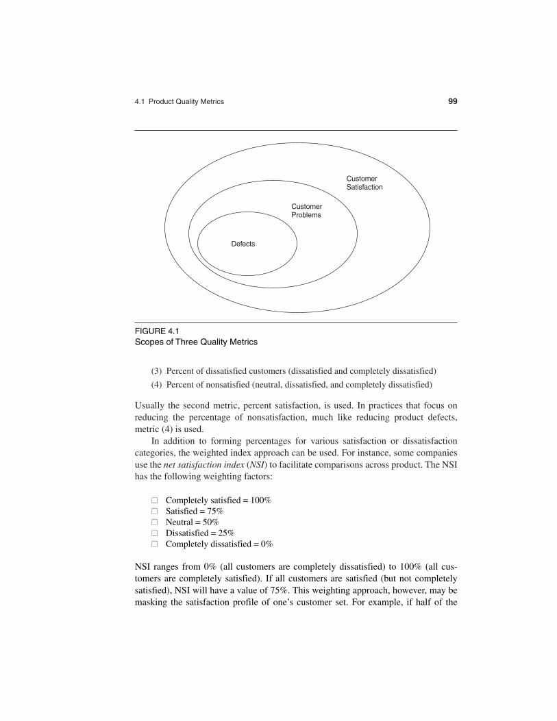
customer satisfaction, one has to reduce defects and overall problems and, in addi-tion, manage factors of broader scope such as timing and availability of the product,company image, services, total customer solutions, and so forth. From the softwarequality standpoint, the relationship of the scopes of the three metrics can be repre-sented by the Venn diagram in Figure 4.1.
4.1.3 Customer Satisfaction Metrics
Customer satisfaction is often measured by customer survey data via the five-pointscale:
�� Very satisfied�� Satisfied�� Neutral�� Dissatisfied�� Very dissatisfied.
Satisfaction with the overall quality of the product and its specific dimensions is usu-ally obtained through various methods of customer surveys. For example, the spe-cific parameters of customer satisfaction in software monitored by IBM include theCUPRIMDSO categories (capability, functionality, usability, performance, reliabil-ity, installability, maintainability, documentation/information, service, and overall);for Hewlett-Packard they are FURPS (functionality, usability, reliability, perfor-mance, and service).
Based on the five-point-scale data, several metrics with slight variations can beconstructed and used, depending on the purpose of analysis. For example:
(1) Percent of completely satisfied customers
(2) Percent of satisfied customers (satisfied and completely satisfied)
98 Chapter 4: Software Quality Metrics Overview
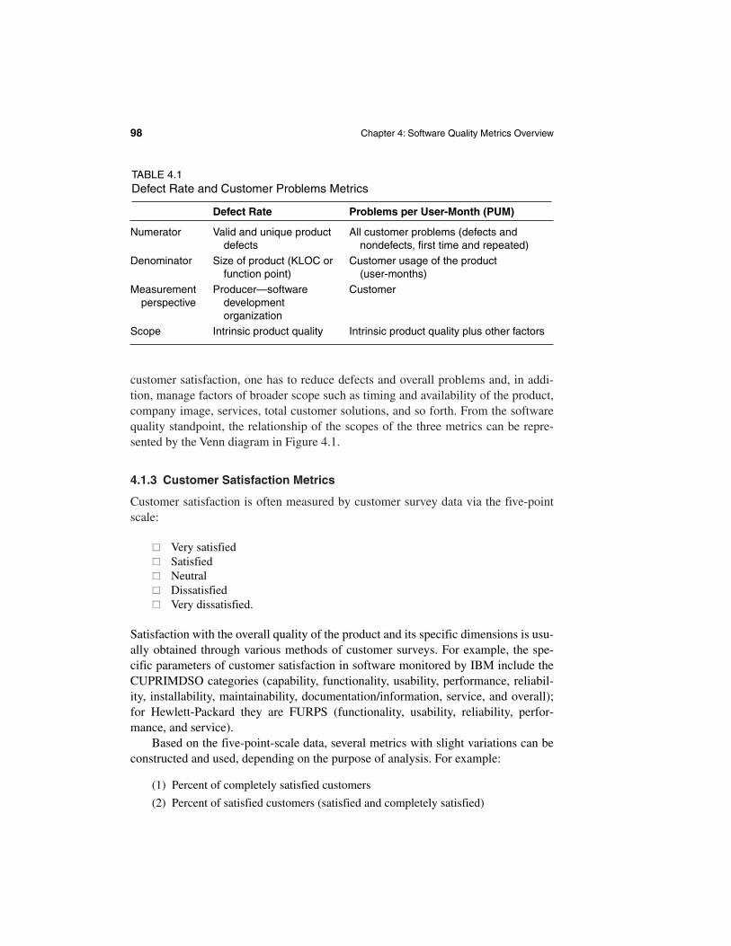
TABLE 4.1Defect Rate and Customer Problems Metrics
Defect Rate Problems per User-Month (PUM)
Numerator Valid and unique product All customer problems (defects and defects nondefects, first time and repeated)
Denominator Size of product (KLOC or Customer usage of the product function point) (user-months)
Measurement Producer—software Customerperspective development
organizationScope Intrinsic product quality Intrinsic product quality plus other factors
4.1 Product Quality Metrics 99
(3) Percent of dissatisfied customers (dissatisfied and completely dissatisfied)
(4) Percent of nonsatisfied (neutral, dissatisfied, and completely dissatisfied)
Usually the second metric, percent satisfaction, is used. In practices that focus onreducing the percentage of nonsatisfaction, much like reducing product defects,metric (4) is used.
In addition to forming percentages for various satisfaction or dissatisfactioncategories, the weighted index approach can be used. For instance, some companiesuse the net satisfaction index (NSI) to facilitate comparisons across product. The NSIhas the following weighting factors:
�� Completely satisfied = 100%�� Satisfied = 75%�� Neutral = 50%�� Dissatisfied = 25%�� Completely dissatisfied = 0%
NSI ranges from 0% (all customers are completely dissatisfied) to 100% (all cus-tomers are completely satisfied). If all customers are satisfied (but not completelysatisfied), NSI will have a value of 75%. This weighting approach, however, may bemasking the satisfaction profile of one’s customer set. For example, if half of the
CustomerSatisfaction
CustomerProblems
Defects
FIGURE 4.1Scopes of Three Quality Metrics
customers are completely satisfied and half are neutral, NSI’s value is also 75%,which is equivalent to the scenario that all customers are satisfied. If satisfaction is agood indicator of product loyalty, then half completely satisfied and half neutral iscertainly less positive than all satisfied. Furthermore, we are not sure of the rationalebehind giving a 25% weight to those who are dissatisfied. Therefore, this example ofNSI is not a good metric; it is inferior to the simple approach of calculating percent-age of specific categories. If the entire satisfaction profile is desired, one can simplyshow the percent distribution of all categories via a histogram. A weighted index isfor data summary when multiple indicators are too cumbersome to be shown. Forexample, if customers’ purchase decisions can be expressed as a function of their sat-isfaction with specific dimensions of a product, then a purchase decision index couldbe useful. In contrast, if simple indicators can do the job, then the weighted indexapproach should be avoided.
4.2 In-Process Quality Metrics
Because our goal is to understand the programming process and to learn to engineerquality into the process, in-process quality metrics play an important role. In-processquality metrics are less formally defined than end-product metrics, and their prac-tices vary greatly among software developers. On the one hand, in-process qualitymetrics simply means tracking defect arrival during formal machine testing for someorganizations. On the other hand, some software organizations with well-establishedsoftware metrics programs cover various parameters in each phase of the develop-ment cycle. In this section we briefly discuss several metrics that are basic to soundin-process quality management. In later chapters on modeling we will examine someof them in greater detail and discuss others within the context of models.
4.2.1 Defect Density During Machine Testing
Defect rate during formal machine testing (testing after code is integrated into thesystem library) is usually positively correlated with the defect rate in the field.Higher defect rates found during testing is an indicator that the software has experi-enced higher error injection during its development process, unless the higher testingdefect rate is due to an extraordinary testing effort—for example, additional testingor a new testing approach that was deemed more effective in detecting defects. Therationale for the positive correlation is simple: Software defect density never followsthe uniform distribution. If a piece of code or a product has higher testing defects, itis a result of more effective testing or it is because of higher latent defects in thecode. Myers (1979) discusses a counterintuitive principle that the more defects foundduring testing, the more defects will be found later. That principle is another expres-
100 Chapter 4: Software Quality Metrics Overview
4.2 In-process Quality Metrics 101
sion of the positive correlation between defect rates during testing and in the field orbetween defect rates between phases of testing.
This simple metric of defects per KLOC or function point, therefore, is a goodindicator of quality while the software is still being tested. It is especially useful tomonitor subsequent releases of a product in the same development organization.Therefore, release-to-release comparisons are not contaminated by extraneous fac-tors. The development team or the project manager can use the following scenarios tojudge the release quality:
�� If the defect rate during testing is the same or lower than that of the previousrelease (or a similar product), then ask: Does the testing for the current releasedeteriorate?
• If the answer is no, the quality perspective is positive.• If the answer is yes, you need to do extra testing (e.g., add test cases to
increase coverage, blitz test, customer testing, stress testing, etc.).
�� If the defect rate during testing is substantially higher than that of the previousrelease (or a similar product), then ask: Did we plan for and actually improvetesting effectiveness?
• If the answer is no, the quality perspective is negative. Ironically, the onlyremedial approach that can be taken at this stage of the life cycle is to domore testing, which will yield even higher defect rates.
• If the answer is yes, then the quality perspective is the same or positive.
4.2.2 Defect Arrival Pattern During Machine Testing
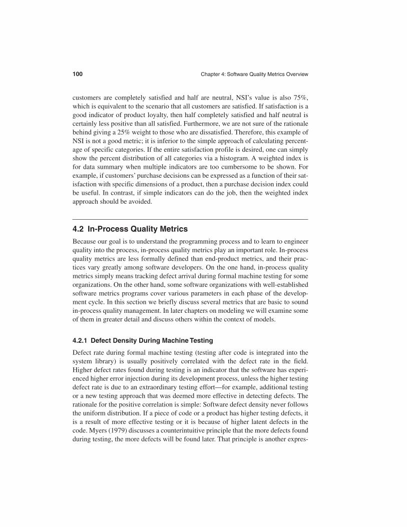
Overall defect density during testing is a summary indicator. The pattern of defectarrivals (or for that matter, times between failures) gives more information. Evenwith the same overall defect rate during testing, different patterns of defect arrivalsindicate different quality levels in the field. Figure 4.2 shows two contrasting pat-terns for both the defect arrival rate and the cumulative defect rate. Data were plotted from 44 weeks before code-freeze until the week prior to code-freeze. Thesecond pattern, represented by the charts on the right side, obviously indicates that testing started late, the test suite was not sufficient, and that the testing endedprematurely.
The objective is always to look for defect arrivals that stabilize at a very lowlevel, or times between failures that are far apart, before ending the testing effort andreleasing the software to the field. Such declining patterns of defect arrival duringtesting are indeed the basic assumption of many software reliability models. Thetime unit for observing the arrival pattern is usually weeks and occasionally months.For reliability models that require execution time data, the time interval is in units ofCPU time.
When we talk about the defect arrival pattern during testing, there are actuallythree slightly different metrics, which should be looked at simultaneously:
�� The defect arrivals (defects reported) during the testing phase by time interval(e.g., week). These are the raw number of arrivals, not all of which are validdefects.
�� The pattern of valid defect arrivals—when problem determination is done onthe reported problems. This is the true defect pattern.
�� The pattern of defect backlog overtime. This metric is needed because develop-ment organizations cannot investigate and fix all reported problems immedi-ately. This metric is a workload statement as well as a quality statement. If the defect backlog is large at the end of the development cycle and a lot of fixes have yet to be integrated into the system, the stability of the system (hence its quality) will be affected. Retesting (regression test) is needed toensure that targeted product quality levels are reached.
102 Chapter 4: Software Quality Metrics Overview
Week Week
WeekWeek
Test
Def
ect A
rriv
al R
ate
Test
Def
ect A
rriv
al R
ate
Test
Def
ect C
UM
Rat
e
Test
Def
ect C
UM
Rat
e
FIGURE 4.2Two Contrasting Defect Arrival Patterns During Testing
4.2 In-process Quality Metrics 103
4.2.3 Phase-Based Defect Removal Pattern
The phase-based defect removal pattern is an extension of the test defect densitymetric. In addition to testing, it requires the tracking of defects at all phases of thedevelopment cycle, including the design reviews, code inspections, and formal veri-fications before testing. Because a large percentage of programming defects is re-lated to design problems, conducting formal reviews or functional verifications toenhance the defect removal capability of the process at the front end reduces errorinjection. The pattern of phase-based defect removal reflects the overall defectremoval ability of the development process.
With regard to the metrics for the design and coding phases, in addition to defectrates, many development organizations use metrics such as inspection coverage andinspection effort for in-process quality management. Some companies even set up“model values” and “control boundaries” for various in-process quality indicators.For example, Cusumano (1992) reports the specific model values and control bound-aries for metrics such as review coverage rate, review manpower rate (review workhours/number of design work hours), defect rate, and so forth, which were used byNEC’s Switching Systems Division.
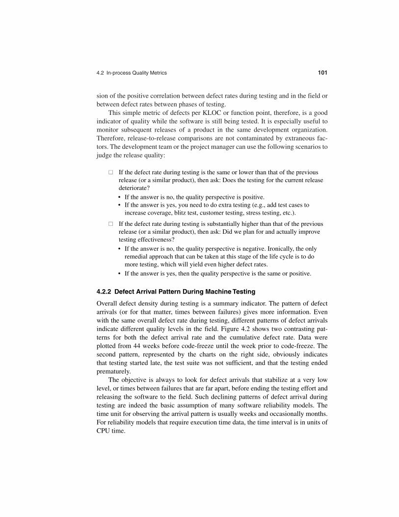
Figure 4.3 shows the patterns of defect removal of two development projects:project A was front-end loaded and project B was heavily testing-dependent forremoving defects. In the figure, the various phases of defect removal are high-leveldesign review (I0), low-level design review (I1), code inspection (I2), unit test (UT),component test (CT), and system test (ST). As expected, the field quality of project Aoutperformed project B significantly.
4.2.4 Defect Removal Effectiveness
Defect removal effectiveness (or efficiency, as used by some writers) can be definedas follows:
Because the total number of latent defects in the product at any given phase isnot known, the denominator of the metric can only be approximated. It is usuallyestimated by:
Defects removed during the phase + defects found later
The metric can be calculated for the entire development process, for the front end (before code integration), and for each phase. It is called early defect removal
DREDefects removed during a development phase
Defects latent in the product= ×100%
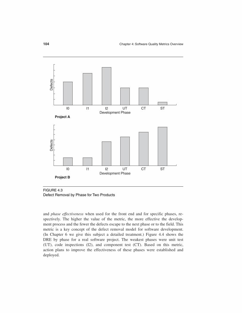
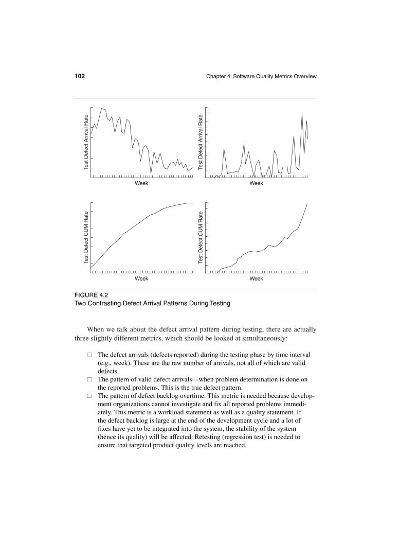
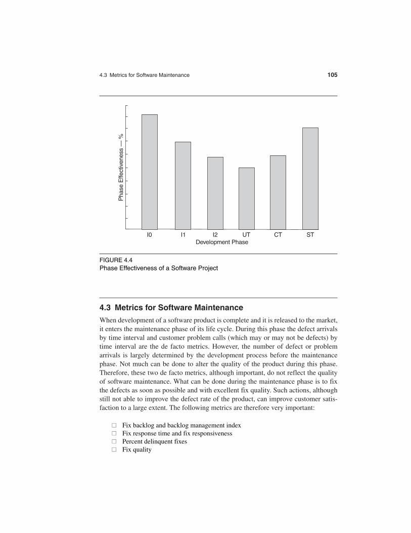
and phase effectiveness when used for the front end and for specific phases, re-spectively. The higher the value of the metric, the more effective the develop-ment process and the fewer the defects escape to the next phase or to the field. Thismetric is a key concept of the defect removal model for software development. (In Chapter 6 we give this subject a detailed treatment.) Figure 4.4 shows the DRE by phase for a real software project. The weakest phases were unit test (UT), code inspections (I2), and component test (CT). Based on this metric,action plans to improve the effectiveness of these phases were established anddeployed.
104 Chapter 4: Software Quality Metrics Overview
Development PhaseI0 I1 I2 UT CT ST
Development PhaseI0 I1 I2 UT CT ST
Def
ects
Def
ects
Project A
Project B
FIGURE 4.3Defect Removal by Phase for Two Products
4.3 Metrics for Software Maintenance 105
4.3 Metrics for Software Maintenance
When development of a software product is complete and it is released to the market,it enters the maintenance phase of its life cycle. During this phase the defect arrivalsby time interval and customer problem calls (which may or may not be defects) bytime interval are the de facto metrics. However, the number of defect or problemarrivals is largely determined by the development process before the maintenancephase. Not much can be done to alter the quality of the product during this phase.Therefore, these two de facto metrics, although important, do not reflect the qualityof software maintenance. What can be done during the maintenance phase is to fixthe defects as soon as possible and with excellent fix quality. Such actions, althoughstill not able to improve the defect rate of the product, can improve customer satis-faction to a large extent. The following metrics are therefore very important:
�� Fix backlog and backlog management index�� Fix response time and fix responsiveness�� Percent delinquent fixes�� Fix quality
Development PhaseI0 I1 I2 UT CT ST
Pha
se E
ffect
iven
ess
— %
FIGURE 4.4Phase Effectiveness of a Software Project
4.3.1 Fix Backlog and Backlog Management Index
Fix backlog is a workload statement for software maintenance. It is related to boththe rate of defect arrivals and the rate at which fixes for reported problems becomeavailable. It is a simple count of reported problems that remain at the end of eachmonth or each week. Using it in the format of a trend chart, this metric can providemeaningful information for managing the maintenance process. Another metric tomanage the backlog of open, unresolved, problems is the backlog management index(BMI).
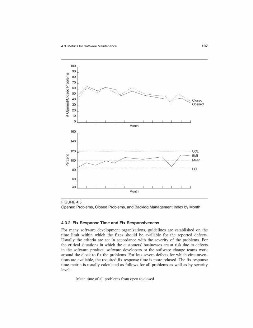
As a ratio of number of closed, or solved, problems to number of problemarrivals during the month, if BMI is larger than 100, it means the backlog is reduced.If BMI is less than 100, then the backlog increased. With enough data points, thetechniques of control charting can be used to calculate the backlog managementcapability of the maintenance process. More investigation and analysis should betriggered when the value of BMI exceeds the control limits. Of course, the goal isalways to strive for a BMI larger than 100. A BMI trend chart or control chart shouldbe examined together with trend charts of defect arrivals, defects fixed (closed), andthe number of problems in the backlog.
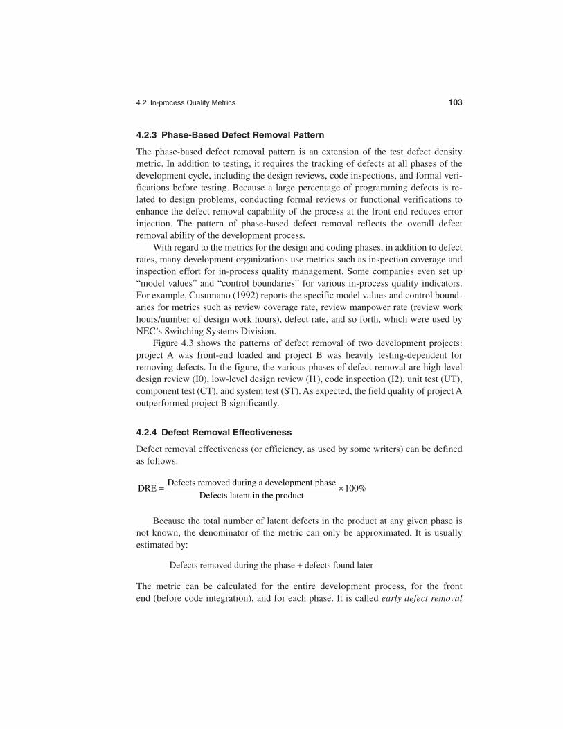
Figure 4.5 is a trend chart by month of the numbers of opened and closed prob-lems of a software product, and a pseudo-control chart for the BMI. The latest releaseof the product was available to customers in the month for the first data points on thetwo charts. This explains the rise and fall of the problem arrivals and closures. Themean BMI was 102.9%, indicating that the capability of the fix process was func-tioning normally. All BMI values were within the upper (UCL) and lower (LCL)control limits—the backlog management process was in control. (Note: We call theBMI chart a pseudo-control chart because the BMI data are autocorrelated and there-fore the assumption of independence for control charts is violated. Despite not being“real” control charts in statistical terms, however, we found pseudo-control chartssuch as the BMI chart quite useful in software quality management. In Chapter 5 weprovide more discussions and examples.)
A variation of the problem backlog index is the ratio of number of opened prob-lems (problem backlog) to number of problem arrivals during the month. If the indexis 1, that means the team maintains a backlog the same as the problem arrival rate. Ifthe index is below 1, that means the team is fixing problems faster than the problemarrival rate. If the index is higher than 1, that means the team is losing ground in theirproblem-fixing capability relative to problem arrivals. Therefore, this variant index isalso a statement of fix responsiveness.
106 Chapter 4: Software Quality Metrics Overview
BMINumber of problems closed during the month
Number of problem arrivals during the month= ×100%
4.3 Metrics for Software Maintenance 107
4.3.2 Fix Response Time and Fix Responsiveness
For many software development organizations, guidelines are established on the time limit within which the fixes should be available for the reported defects. Usually the criteria are set in accordance with the severity of the problems. For the critical situations in which the customers’ businesses are at risk due to defects in the software product, software developers or the software change teams workaround the clock to fix the problems. For less severe defects for which circumven-tions are available, the required fix response time is more relaxed. The fix responsetime metric is usually calculated as follows for all problems as well as by severitylevel:
Mean time of all problems from open to closed
Month
100
90
80
70
60
50
40
30
20
10
0
ClosedOpened
Month
160
140
120
100
80
60
40
UCLBMIMean
LCL
Per
cent
# O
pene
d/C
lose
d P
robl
ems
FIGURE 4.5Opened Problems, Closed Problems, and Backlog Management Index by Month
If there are data points with extreme values, medians should be used instead of mean.Such cases could occur for less severe problems for which customers may be satis-fied with the circumvention and didn’t demand a fix. Therefore, the problem mayremain open for a long time in the tracking report.
In general, short fix response time leads to customer satisfaction. However, thereis a subtle difference between fix responsiveness and short fix response time. Fromthe customer’s perspective, the use of averages may mask individual differences. Theimportant elements of fix responsiveness are customer expectations, the agreed-to fixtime, and the ability to meet one’s commitment to the customer. For example, Johntakes his car to the dealer for servicing in the early morning and needs it back bynoon. If the dealer promises noon but does not get the car ready until 2 o’clock, Johnwill not be a satisfied customer. On the other hand, Julia does not need her mini vanback until she gets off from work, around 6 P.M. As long as the dealer finishes servic-ing her van by then, Julia is a satisfied customer. If the dealer leaves a timely phonemessage on her answering machine at work saying that her van is ready to pick up,Julia will be even more satisfied. This type of fix responsiveness process is indeedbeing practiced by automobile dealers who focus on customer satisfaction.
In this writer’s knowledge, the systems software development of Hewlett-Packard (HP) in California and IBM Rochester’s systems software development havefix responsiveness processes similar to the process just illustrated by the automobileexamples. In fact, IBM Rochester’s practice originated from a benchmarkingexchange with HP some years ago. The metric for IBM Rochester’s fix responsive-ness is operationalized as percentage of delivered fixes meeting committed dates tocustomers.
4.3.3 Percent Delinquent Fixes
The mean (or median) response time metric is a central tendency measure. A moresensitive metric is the percentage of delinquent fixes. For each fix, if the turnaroundtime greatly exceeds the required response time, then it is classified as delinquent:
This metric, however, is not a metric for real-time delinquent management because itis for closed problems only. Problems that are still open must be factored into the cal-culation for a real-time metric. Assuming the time unit is 1 week, we propose that thepercent delinquent of problems in the active backlog be used. Active backlog refers toall opened problems for the week, which is the sum of the existing backlog at the
108 Chapter 4: Software Quality Metrics Overview
Percent delinquent fixes
Number of fixes that exceeded theresponse time criteria by severity level
Number of fixesdelivered in a specified time
= × 100%
4.3 Metrics for Software Maintenance 109
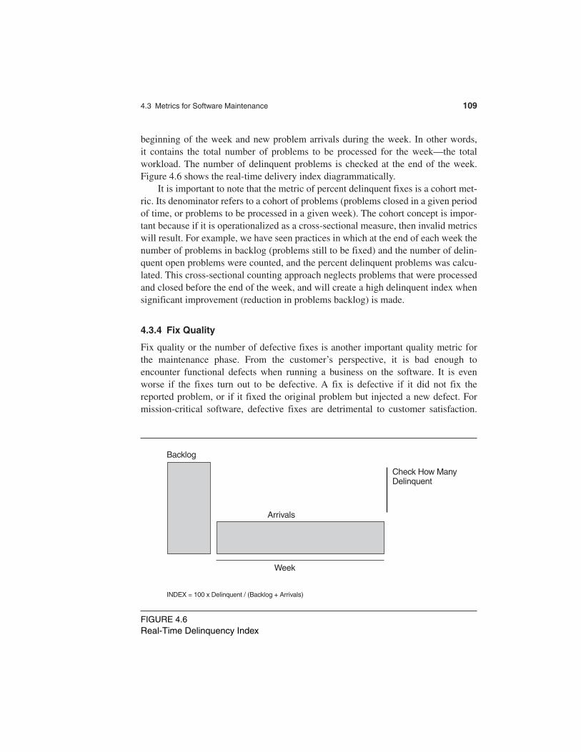
beginning of the week and new problem arrivals during the week. In other words,it contains the total number of problems to be processed for the week—the totalworkload. The number of delinquent problems is checked at the end of the week.Figure 4.6 shows the real-time delivery index diagrammatically.
It is important to note that the metric of percent delinquent fixes is a cohort met-ric. Its denominator refers to a cohort of problems (problems closed in a given periodof time, or problems to be processed in a given week). The cohort concept is impor-tant because if it is operationalized as a cross-sectional measure, then invalid metricswill result. For example, we have seen practices in which at the end of each week thenumber of problems in backlog (problems still to be fixed) and the number of delin-quent open problems were counted, and the percent delinquent problems was calcu-lated. This cross-sectional counting approach neglects problems that were processedand closed before the end of the week, and will create a high delinquent index whensignificant improvement (reduction in problems backlog) is made.
4.3.4 Fix Quality
Fix quality or the number of defective fixes is another important quality metric forthe maintenance phase. From the customer’s perspective, it is bad enough toencounter functional defects when running a business on the software. It is evenworse if the fixes turn out to be defective. A fix is defective if it did not fix thereported problem, or if it fixed the original problem but injected a new defect. Formission-critical software, defective fixes are detrimental to customer satisfaction.
Backlog
Check How ManyDelinquent
INDEX = 100 x Delinquent / (Backlog + Arrivals)
Week
Arrivals
FIGURE 4.6Real-Time Delinquency Index

The metric of percent defective fixes is simply the percentage of all fixes in a timeinterval (e.g., 1 month) that are defective.
A defective fix can be recorded in two ways: Record it in the month it was dis-covered or record it in the month the fix was delivered. The first is a customer mea-sure, the second is a process measure. The difference between the two dates is thelatent period of the defective fix. It is meaningful to keep track of the latency dataand other information such as the number of customers who were affected by thedefective fix. Usually the longer the latency, the more customers are affected becausethere is more time for customers to apply that defective fix to their software system.
There is an argument against using percentage for defective fixes. If the numberof defects, and therefore the fixes, is large, then the small value of the percentagemetric will show an optimistic picture, although the number of defective fixes couldbe quite large. This metric, therefore, should be a straight count of the number ofdefective fixes. The quality goal for the maintenance process, of course, is zerodefective fixes without delinquency.
4.4 Examples of Metrics Programs
4.4.1 Motorola
Motorola’s software metrics program is well articulated by Daskalantonakis (1992).By following the Goal/Question/Metric paradigm of Basili and Weiss (1984), goalswere identified, questions were formulated in quantifiable terms, and metrics wereestablished. The goals and measurement areas identified by the Motorola QualityPolicy for Software Development (QPSD) are listed in the following.
Goals
�� Goal 1: Improve project planning.�� Goal 2: Increase defect containment.�� Goal 3: Increase software reliability.�� Goal 4: Decrease software defect density.�� Goal 5: Improve customer service.�� Goal 6: Reduce the cost of nonconformance.�� Goal 7: Increase software productivity.
Measurement Areas
�� Delivered defects and delivered defects per size�� Total effectiveness throughout the process�� Adherence to schedule�� Accuracy of estimates�� Number of open customer problems
110 Chapter 4: Software Quality Metrics Overview

4.4 Examples of Metrics Programs 111
�� Time that problems remain open�� Cost of nonconformance�� Software reliability
For each goal the questions to be asked and the corresponding metrics were also for-mulated. In the following, we list the questions and metrics for each goal:1
Goal 1: Improve Project Planning
Question 1.1: What was the accuracy of estimating the actual value of projectschedule?
Metric 1.1 : Schedule Estimation Accuracy (SEA)
Question 1.2: What was the accuracy of estimating the actual value of projecteffort?
Metric 1.2 : Effort Estimation Accuracy (EEA)
Goal 2: Increase Defect Containment
Question 2.1: What is the currently known effectiveness of the defect detectionprocess prior to release?
Metric 2.1: Total Defect Containment Effectiveness (TDCE)
Question 2.2: What is the currently known containment effectiveness of faults intro-duced during each constructive phase of software development for a particular soft-ware product?
Metric 2.2: Phase Containment Effectiveness for phase i (PCEi)
1. Source: From Daskalantonakis, M. K., “A Practical View of Software Measurement and Implement-ation Experiences Within Motorola (1001–1004),” IEEE Transactions on Software Engineering, Vol.18, No. 11 (November 1992): 998–1010. Copyright © IEEE, 1992. Used with permission to reprint.
SEAActual project duration
Estimated project duration=
EEAActual project effort
Estimated project effort=
TDCENumber of prerelease defects
Number of prerelease defects+ Number of postrelease defects
=
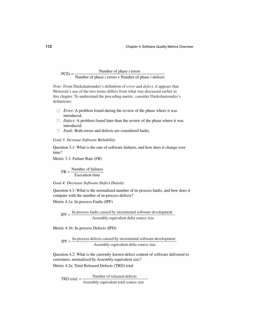
Note: From Daskalantonakis’s definition of error and defect, it appears thatMotorola’s use of the two terms differs from what was discussed earlier in this chapter. To understand the preceding metric, consider Daskalantonakis’s definitions:
�� Error: A problem found during the review of the phase where it was introduced.
�� Defect: A problem found later than the review of the phase where it wasintroduced.
�� Fault: Both errors and defects are considered faults.
Goal 3: Increase Software Reliability
Question 3.1: What is the rate of software failures, and how does it change overtime?
Metric 3.1: Failure Rate (FR)
Goal 4: Decrease Software Defect Density
Question 4.1: What is the normalized number of in-process faults, and how does itcompare with the number of in-process defects?
Metric 4.1a: In-process Faults (IPF)
Metric 4.1b: In-process Defects (IPD)
Question 4.2: What is the currently known defect content of software delivered tocustomers, normalized by Assembly-equivalent size?
Metric 4.2a: Total Released Defects (TRD) total
112 Chapter 4: Software Quality Metrics Overview
PCEiNumber of phase errors
Number of phase errors + Number of phase defects= i
i i
FRNumber of failures
Execution time=
IPFIn-process faults caused by incremental software development
Assembly-equivalent delta source size=
IPFIn-process defects caused by incremental software development
Assembly-equivalent delta source size=
TRD totalNumber of released defects
Assembly-equivalent total source size=
4.4 Examples of Metrics Programs 113
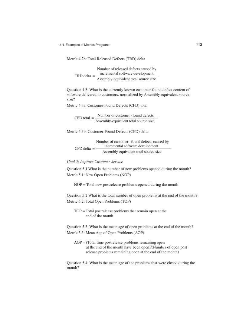
Metric 4.2b: Total Released Defects (TRD) delta
Question 4.3: What is the currently known customer-found defect content of software delivered to customers, normalized by Assembly-equivalent source size?
Metric 4.3a: Customer-Found Defects (CFD) total
Metric 4.3b: Customer-Found Defects (CFD) delta
Goal 5: Improve Customer Service
Question 5.1 What is the number of new problems opened during the month?
Metric 5.1: New Open Problems (NOP)
NOP = Total new postrelease problems opened during the month
Question 5.2 What is the total number of open problems at the end of the month?
Metric 5.2: Total Open Problems (TOP)
TOP = Total postrelease problems that remain open at theend of the month
Question 5.3: What is the mean age of open problems at the end of the month?
Metric 5.3: Mean Age of Open Problems (AOP)
AOP = (Total time postrelease problems remaining openat the end of the month have been open)/(Number of open postrelease problems remaining open at the end of the month)
Question 5.4: What is the mean age of the problems that were closed during themonth?
TRD delta
Number of released defects caused byincremental software development
Assembly-equivalent total source size=
CFD totalNumber of customer -found defects
Assembly-equivalent total source size=
CFD delta
Number of customer -found defects caused byincremental software development
Assembly-equivalent total source size=
Metric 5.4: Mean Age of Closed Problems (ACP)
ACP = (Total time postrelease problems closed withinthe month were open)/(Number of open postrelease problems closed within the month)
Goal 6: Reduce the Cost of Nonconformance
Question 6.1: What was the cost to fix postrelease problems during the month?
Metric 6.1: Cost of Fixing Problems (CFP)
CFP = Dollar cost associated with fixing postreleaseproblems within the month
Goal 7: Increase Software Productivity
Question 7.1: What was the productivity of software development projects (basedon source size)?
Metric 7.1a: Software Productivity total (SP total)
Metric 7.1b: Software Productivity delta (SP delta)
From the preceding goals one can see that metrics 3.1, 4.2a, 4.2b, 4.3a, and 4.3bare metrics for end-product quality, metrics 5.1 through 5.4 are metrics for softwaremaintenance, and metrics 2.1, 2.2, 4.1a, and 4.1b are in-process quality metrics. Theothers are for scheduling, estimation, and productivity.
In addition to the preceding metrics, which are defined by the Motorola Soft-ware Engineering Process Group (SEPG), Daskalantonakis describes in-processmetrics that can be used for schedule, project, and quality control. Without gettinginto too many details, we list these additional in-process metrics in the following.[For details and other information about Motorola’s software metrics program,see Daskalantonakis’s original article (1992).] Items 1 through 4 are for projectstatus/control and items 5 through 7 are really in-process quality metrics that canprovide information about the status of the project and lead to possible actions forfurther quality improvement.
1. Life-cycle phase and schedule tracking metric: Track schedule based on life-cycle phase and compare actual to plan.
114 Chapter 4: Software Quality Metrics Overview
SP totalAssembly-equivalent total source size
Software development effort=
SP deltaAssembly-equivalent delta source size
Software development effort=
4.4 Examples of Metrics Programs 115
2. Cost/earned value tracking metric: Track actual cumulative cost of the projectversus budgeted cost, and actual cost of the project so far, with continuousupdate throughout the project.
3. Requirements tracking metric: Track the number of requirements change at theproject level.
4. Design tracking metric: Track the number of requirements implemented indesign versus the number of requirements written.
5. Fault-type tracking metric: Track causes of faults.6. Remaining defect metrics: Track faults per month for the project and use
Rayleigh curve to project the number of faults in the months ahead duringdevelopment.
7. Review effectiveness metric: Track error density by stages of review and usecontrol chart methods to flag the exceptionally high or low data points.
4.4.2 Hewlett-Packard
Grady and Caswell (1986) offer a good description of Hewlett-Packard’s softwaremetric program, including both the primitive metrics and computed metrics that arewidely used at HP. Primitive metrics are those that are directly measurable andaccountable such as control token, data token, defect, total operands, LOC, and soforth. Computed metrics are metrics that are mathematical combinations of two ormore primitive metrics. The following is an excerpt of HP’s computed metrics:2
Average fixed defects/working day: self-explanatory.
Average engineering hours/fixed defect: self-explanatory.
Average reported defects/working day: self-explanatory.
Bang: “A quantitative indicator of net usable function from the user’s point ofview” (DeMarco, 1982). There are two methods for computing Bang. Compu-tation of Bang for function-strong systems involves counting the tokens enter-ing and leaving the function multiplied by the weight of the function. Fordata-strong systems it involves counting the objects in the database weightedby the number of relationships of which the object is a member.
Branches covered/total branches: When running a program, this metric indi-cates what percentage of the decision points were actually executed.
Defects/KNCSS: Self-explanatory (KNCSS—Thousand noncomment sourcestatements).
Defects/LOD: Self-explanatory (LOD—Lines of documentation not includedin program source code).
Defects/testing time: Self-explanatory.
1. Source: Grady, R. B., and D. L. Caswell, Software Metrics: Establishing A Company-Wide Program,pp. 225–226. Englewood Cliffs, N.J.: Prentice-Hall. Copyright © 1986 Prentice-Hall, Inc. Used withpermission to reprint.
Design weight: “Design weight is a simple sum of the module weights over theset of all modules in the design” (DeMarco, 1982). Each module weight is afunction of the token count associated with the module and the expected num-ber of decision counts which are based on the structure of data.
NCSS/engineering month: Self-explanatory.
Percent overtime: Average overtime/40 hours per week.
Phase: engineering months/total engineering months: Self-explanatory.
Of these metrics, defects/KNCSS and defects/LOD are end-product quality metrics.Defects/testing time is a statement of testing effectiveness, and branches covered/total branches is testing coverage in terms of decision points. Therefore, both aremeaningful in-process quality metrics. Bang is a measurement of functions andNCSS/engineering month is a productivity measure. Design weight is an interestingmeasurement but its use is not clear. The other metrics are for workload, schedule,project control, and cost of defects.
As Grady and Caswell point out, this list represents the most widely used com-puted metrics at HP, but it may not be comprehensive. For instance, many others arediscussed in other sections of their book. For example, customer satisfaction mea-surements in relation to software quality attributes are a key area in HP’s softwaremetrics. As mentioned earlier in this chapter, the software quality attributes definedby HP are called FURPS (functionality, usability, reliability, performance, and sup-portability). Goals and objectives for FURPS are set for software projects.Furthermore, to achieve the FURPS goals of the end product, measurable objectivesusing FURPS for each life-cycle phase are also set (Grady and Caswell, 1986,pp. 159–162).
MacLeod (1993) describes the implementation and sustenance of a softwareinspection program in an HP division. The metrics used include average hours perinspection, average defects per inspection, average hours per defect, and defectcauses. These inspection metrics, used appropriately in the proper context (e.g., com-paring the current project with previous projects), can be used to monitor the inspec-tion phase (front end) of the software development process.
4.4.3 IBM Rochester
Because many examples of the metrics used at IBM Rochester have already beendiscussed or will be elaborated on later, here we give just an overview. Furthermore,we list only selected quality metrics; metrics related to project management, produc-tivity, scheduling, costs, and resources are not included.
�� Overall customer satisfaction as well as satisfaction with various quality attrib-utes such as CUPRIMDS (capability, usability, performance, reliability, install,maintenance, documentation/information, and service).
116 Chapter 4: Software Quality Metrics Overview
4.5 Collecting Software Engineering Data 117
�� Postrelease defect rates such as those discussed in section 4.1.1.�� Customer problem calls per month�� Fix response time�� Number of defective fixes�� Backlog management index�� Postrelease arrival patterns for defects and problems (both defects and
non-defect-oriented problems)�� Defect removal model for the software development process �� Phase effectiveness (for each phase of inspection and testing)�� Inspection coverage and effort �� Compile failures and build/integration defects�� Weekly defect arrivals and backlog during testing�� Defect severity�� Defect cause and problem component analysis�� Reliability: mean time to initial program loading (IPL) during testing�� Stress level of the system during testing as measured in level of CPU use in
terms of number of CPU hours per system per day during stress testing�� Number of system crashes and hangs during stress testing and system testing�� Models for postrelease defect estimation�� Various customer feedback metrics at the end of the development cycle before
the product is shipped �� S curves for project progress comparing actual to plan for each phase of devel-
opment such as number of inspections conducted by week, LOC integrated byweek, number of test cases attempted and succeeded by week, and so forth.
4.5 Collecting Software Engineering Data
The challenge of collecting software engineering data is to make sure that the col-lected data can provide useful information for project, process, and quality manage-ment and, at the same time, that the data collection process will not be a burden ondevelopment teams. Therefore, it is important to consider carefully what data to col-lect. The data must be based on well-defined metrics and models, which are used todrive improvements. Therefore, the goals of the data collection should be establishedand the questions of interest should be defined before any data is collected. Dataclassification schemes to be used and the level of precision must be carefully speci-fied. The collection form or template and data fields should be pretested. The amountof data to be collected and the number of metrics to be used need not be overwhelm-ing. It is more important that the information extracted from the data be focused,accurate, and useful than that it be plentiful. Without being metrics driven, over-collection of data could be wasteful. Overcollection of data is quite common whenpeople start to measure software without an a priori specification of purpose, objec-tives, profound versus trivial issues, and metrics and models.
Gathering software engineering data can be expensive, especially if it is doneas part of a research program, For example, the NASA Software EngineeringLaboratory spent about 15% of their development costs on gathering and processingdata on hundreds of metrics for a number of projects (Shooman, 1983). For largecommercial development organizations, the relative cost of data gathering and pro-cessing should be much lower because of economy of scale and fewer metrics.However, the cost of data collection will never be insignificant. Nonetheless, datacollection and analysis, which yields intelligence about the project and the develop-ment process, is vital for business success. Indeed, in many organizations, a trackingand data collection system is often an integral part of the software configuration orthe project management system, without which the chance of success of large andcomplex projects will be reduced.
Basili and Weiss (1984) propose a data collection methodology that could beapplicable anywhere. The schema consists of six steps with considerable feedbackand iteration occurring at several places:
1. Establish the goal of the data collection.2. Develop a list of questions of interest.3. Establish data categories.4. Design and test data collection forms.5. Collect and validate data.6. Analyze data.
The importance of the validation element of a data collection system or a develop-ment tracking system cannot be overemphasized.
In their study of NASA’s Software Engineering Laboratory projects, Basili andWeiss (1984) found that software data are error-prone and that special validation pro-visions are generally needed. Validation should be performed concurrently with soft-ware development and data collection, based on interviews with those peoplesupplying the data. In cases where data collection is part of the configuration controlprocess and automated tools are available, data validation routines (e.g., consistencycheck, range limits, conditional entries, etc.) should be an integral part of the tools.Furthermore, training, clear guidelines and instructions, and an understanding ofhow the data are used by people who enter or collect the data enhance data accuracysignificantly.
The actual collection process can take several basic formats such as reportingforms, interviews, and automatic collection using the computer system. For datacollection to be efficient and effective, it should be merged with the configura-tion management or change control system. This is the case in most large develop-ment organizations. For example, at IBM Rochester the change control systemcovers the entire development process, and online tools are used for plan change
118 Chapter 4: Software Quality Metrics Overview
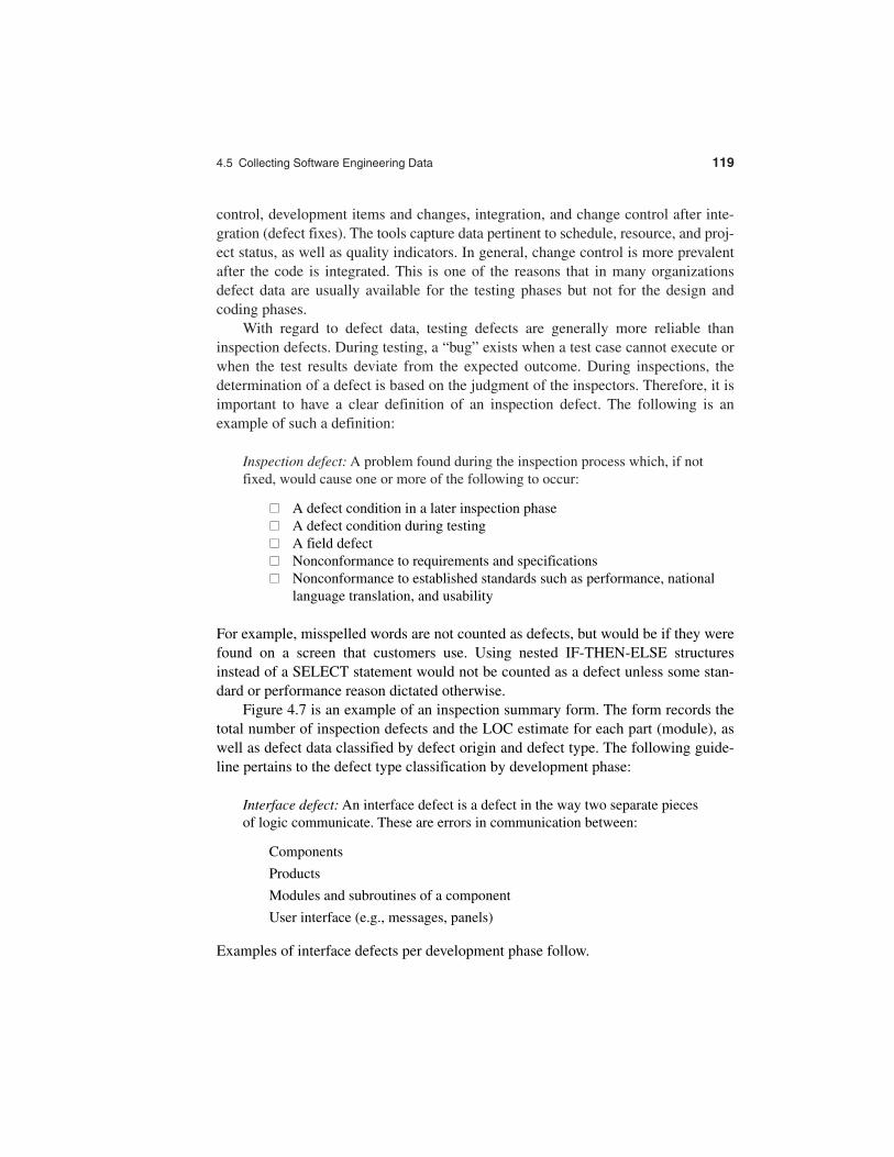
4.5 Collecting Software Engineering Data 119
control, development items and changes, integration, and change control after inte-gration (defect fixes). The tools capture data pertinent to schedule, resource, and proj-ect status, as well as quality indicators. In general, change control is more prevalentafter the code is integrated. This is one of the reasons that in many organizationsdefect data are usually available for the testing phases but not for the design andcoding phases.
With regard to defect data, testing defects are generally more reliable thaninspection defects. During testing, a “bug” exists when a test case cannot execute orwhen the test results deviate from the expected outcome. During inspections, thedetermination of a defect is based on the judgment of the inspectors. Therefore, it isimportant to have a clear definition of an inspection defect. The following is anexample of such a definition:
Inspection defect: A problem found during the inspection process which, if notfixed, would cause one or more of the following to occur:
�� A defect condition in a later inspection phase�� A defect condition during testing�� A field defect�� Nonconformance to requirements and specifications�� Nonconformance to established standards such as performance, national
language translation, and usability
For example, misspelled words are not counted as defects, but would be if they werefound on a screen that customers use. Using nested IF-THEN-ELSE structuresinstead of a SELECT statement would not be counted as a defect unless some stan-dard or performance reason dictated otherwise.
Figure 4.7 is an example of an inspection summary form. The form records thetotal number of inspection defects and the LOC estimate for each part (module), aswell as defect data classified by defect origin and defect type. The following guide-line pertains to the defect type classification by development phase:
Interface defect: An interface defect is a defect in the way two separate piecesof logic communicate. These are errors in communication between:
Components
Products
Modules and subroutines of a component
User interface (e.g., messages, panels)
Examples of interface defects per development phase follow.
High-Level Design (I0)
Use of wrong parameter
Inconsistent use of function keys on user interface (e.g., screen)
Incorrect message used
Presentation of information on screen not usable
120 Chapter 4: Software Quality Metrics Overview
Product: Component: Release:
Inspection Type: (RQ SD IO I1 I2 U1 U2)
Description:
Defect Counts
By Defect OriginRQ SD I0 I1 I2
By Defect TypeLO IF DO Total
Total Preparation Hrs:
Total Persons Attended:
Reinspection Required?
Total Inspection Hrs:
Inspection Date:
Defect Types:DO = DocumentationIF = InterfaceLO = Logic
Defect Origins and Inspection Types:RQ = RequirementsSD = System DesignI0 = High-Level DesignI1 = Low-Level DesignI2 = Code
Tot for Inspection/ Part Name LOC
(Y/N)
/ /
FIGURE 4.7An Inspection Summary Form
4.5 Collecting Software Engineering Data 121
Low-Level Design (I1)
Missing required parameters (e.g., missing parameter on module)
Wrong parameters (e.g., specified incorrect parameter on module)
Intermodule interfaces: input not there, input in wrong order
Intramodule interfaces: passing values/data to subroutines
Incorrect use of common data structures
Misusing data passed to code
Code (I2)
Passing wrong values for parameters on macros, application program interfaces(APIs), modules
Setting up a common control block/area used by another piece of code incorrectly
Not issuing correct exception to caller of code
Logic defect: A logic defect is one that would cause incorrect results in thefunction to be performed by the logic. High-level categories of this type ofdefect are as follows:
Function: capability not implemented or implemented incorrectly
Assignment: initialization
Checking: validate data/values before use
Timing: management of shared/real-time resources
Data Structures: static and dynamic definition of data
Examples of logic defects per development phase follow.
High-Level Design (I0)
Invalid or incorrect screen flow
High-level flow through component missing or incorrect in the review package
Function missing from macros you are implementing
Using a wrong macro to do a function that will not work (e.g., using XXXMSG toreceive a message from a program message queue, instead of YYYMSG).
Missing requirements
Missing parameter/field on command/in database structure/on screen you areimplementing
Wrong value on keyword (e.g., macro, command)
Wrong keyword (e.g., macro, command)

Low-Level Design (I1)
Logic does not implement I0 design
Missing or excessive function
Values in common structure not set
Propagation of authority and adoption of authority (lack of or too much)
Lack of code page conversion
Incorrect initialization
Not handling abnormal termination (conditions, cleanup, exit routines)
Lack of normal termination cleanup
Performance: too much processing in loop that could be moved outside of loop
Code (I2)
Code does not implement I1 design
Lack of initialization
Variables initialized incorrectly
Missing exception monitors
Exception monitors in wrong order
Exception monitors not active
Exception monitors active at the wrong time
Exception monitors set up wrong
Truncating of double-byte character set data incorrectly (e.g., truncating beforeshift in character)
Incorrect code page conversion
Lack of code page conversion
Not handling exceptions/return codes correctly
Documentation defect: A documentation defect is a defect in the description ofthe function (e.g., prologue of macro) that causes someone to do somethingwrong based on this information. For example, if a macro prologue containedan incorrect description of a parameter that caused the user of this macro to usethe parameter incorrectly, this would be a documentation defect against themacro.
Examples of documentation defects per development phase follow.
High-Level Design (I0)
Incorrect information in prologue (e.g., macro)
Misspelling on user interface (e.g., screen)
122 Chapter 4: Software Quality Metrics Overview
4.6. Summary 123
Wrong wording (e.g., messages, command prompt text)
Using restricted words on user interface
Wording in messages, definition of command parameters is technically incorrect
Low-Level Design (I1)
Wrong information in prologue (e.g., macros, program, etc.)
Missing definition of inputs and outputs of module, subroutines, etc.
Insufficient documentation of logic (comments tell what but not why)
Code (I2)
Information in prologue not correct or missing
Wrong wording in messages
Second-level text of message technically incorrect
Insufficient documentation of logic (comments tell what but not why)
Incorrect documentation of logic
4.6 Summary
Software quality metrics focus on the quality aspects of the product, process, andproject. They can be grouped into three categories in accordance with the softwarelife cycle: end-product quality metrics, in-process quality metrics, and maintenancequality metrics. This chapter gives several examples for each category, summarizesthe metrics programs at Motorola, Hewlett-Packard, and IBM Rochester, and dis-cusses data collection.
�� Product quality metrics
–Mean time to failure
–Defect density
–Customer-reported problems
–Customer satisfaction
�� In-process quality metrics
–Phase-based defect removal pattern
–Defect removal effectiveness
–Defect density during formal machine testing
–Defect arrival pattern during formal machine testing
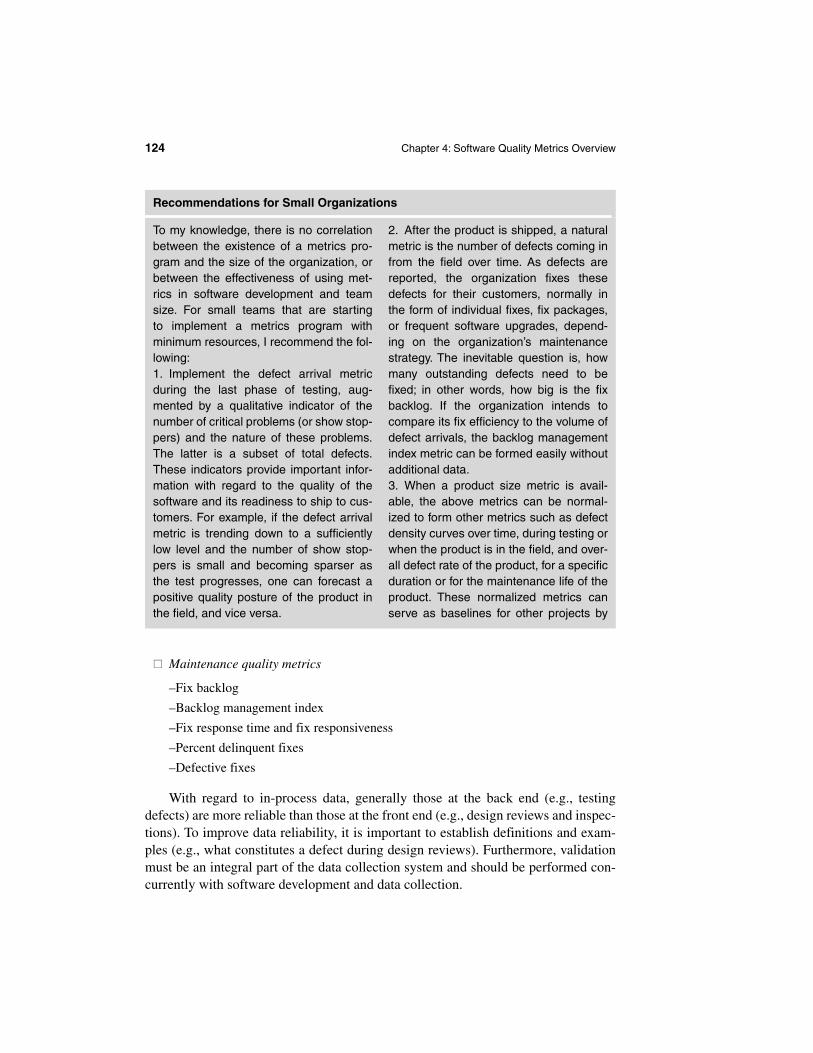
�� Maintenance quality metrics
–Fix backlog
–Backlog management index
–Fix response time and fix responsiveness
–Percent delinquent fixes
–Defective fixes
With regard to in-process data, generally those at the back end (e.g., testingdefects) are more reliable than those at the front end (e.g., design reviews and inspec-tions). To improve data reliability, it is important to establish definitions and exam-ples (e.g., what constitutes a defect during design reviews). Furthermore, validationmust be an integral part of the data collection system and should be performed con-currently with software development and data collection.
124 Chapter 4: Software Quality Metrics Overview
To my knowledge, there is no correlationbetween the existence of a metrics pro-gram and the size of the organization, orbetween the effectiveness of using met-rics in software development and teamsize. For small teams that are starting to implement a metrics program withminimum resources, I recommend the fol-lowing:1. Implement the defect arrival metricduring the last phase of testing, aug-mented by a qualitative indicator of thenumber of critical problems (or show stop-pers) and the nature of these problems.The latter is a subset of total defects.These indicators provide important infor-mation with regard to the quality of thesoftware and its readiness to ship to cus-tomers. For example, if the defect arrivalmetric is trending down to a sufficientlylow level and the number of show stop-pers is small and becoming sparser asthe test progresses, one can forecast apositive quality posture of the product inthe field, and vice versa.
2. After the product is shipped, a naturalmetric is the number of defects coming infrom the field over time. As defects arereported, the organization fixes thesedefects for their customers, normally inthe form of individual fixes, fix packages,or frequent software upgrades, depend-ing on the organization’s maintenancestrategy. The inevitable question is, howmany outstanding defects need to befixed; in other words, how big is the fixbacklog. If the organization intends tocompare its fix efficiency to the volume ofdefect arrivals, the backlog managementindex metric can be formed easily withoutadditional data.3. When a product size metric is avail-able, the above metrics can be normal-ized to form other metrics such as defectdensity curves over time, during testing orwhen the product is in the field, and over-all defect rate of the product, for a specificduration or for the maintenance life of theproduct. These normalized metrics canserve as baselines for other projects by
Recommendations for Small Organizations
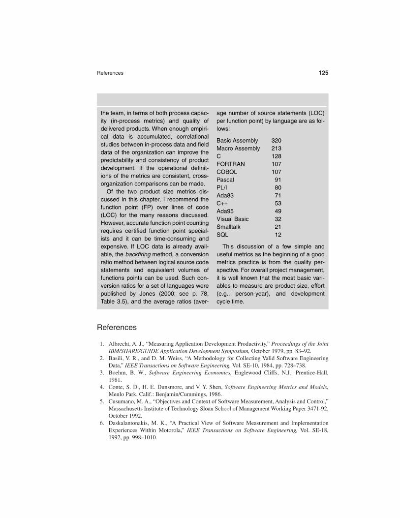
References 125
References
1. Albrecht, A. J., “Measuring Application Development Productivity,” Proceedings of the JointIBM/SHARE/GUIDE Application Development Symposium, October 1979, pp. 83–92.
2. Basili, V. R., and D. M. Weiss, “A Methodology for Collecting Valid Software EngineeringData,” IEEE Transactions on Software Engineering, Vol. SE-10, 1984, pp. 728–738.
3. Boehm, B. W., Software Engineering Economics, Englewood Cliffs, N.J.: Prentice-Hall,1981.
4. Conte, S. D., H. E. Dunsmore, and V. Y. Shen, Software Engineering Metrics and Models,Menlo Park, Calif.: Benjamin/Cummings, 1986.
5. Cusumano, M. A., “Objectives and Context of Software Measurement, Analysis and Control,”Massachusetts Institute of Technology Sloan School of Management Working Paper 3471-92,October 1992.
6. Daskalantonakis, M. K., “A Practical View of Software Measurement and ImplementationExperiences Within Motorola,” IEEE Transactions on Software Engineering, Vol. SE-18,1992, pp. 998–1010.
the team, in terms of both process capac-ity (in-process metrics) and quality ofdelivered products. When enough empiri-cal data is accumulated, correlationalstudies between in-process data and fielddata of the organization can improve thepredictability and consistency of productdevelopment. If the operational definit-ions of the metrics are consistent, cross-organization comparisons can be made.
Of the two product size metrics dis-cussed in this chapter, I recommend thefunction point (FP) over lines of code(LOC) for the many reasons discussed.However, accurate function point countingrequires certified function point special-ists and it can be time-consuming andexpensive. If LOC data is already avail-able, the backfiring method, a conversionratio method between logical source codestatements and equivalent volumes offunctions points can be used. Such con-version ratios for a set of languages werepublished by Jones (2000; see p. 78,Table 3.5), and the average ratios (aver-
age number of source statements (LOC)per function point) by language are as fol-lows:
Basic Assembly 320Macro Assembly 213C 128FORTRAN 107COBOL 107Pascal 91PL/I 80Ada83 71C++ 53Ada95 49Visual Basic 32Smalltalk 21SQL 12
This discussion of a few simple anduseful metrics as the beginning of a goodmetrics practice is from the quality per-spective. For overall project management,it is well known that the most basic vari-ables to measure are product size, effort(e.g., person-year), and developmentcycle time.
7. DeMarco, T., Controlling Software Projects, New York: Yourdon Press, 1982.8. Fenton, N. E., and S. L. Pfleeger, Software Metrics: A Rigorous Approach, 2nd ed., Boston:
International Thomson Computer Press, 1997.9. Grady, R. B., and D. L. Caswell, Software Metrics: Establishing a Company-Wide Program,
Englewood Cliffs, N.J.: Prentice-Hall, 1986.10. IFPUG, IFPUG Counting Practices Manual, Release 4.1, Westerville, Ohio: International
Function Point Users Group, 1999.11. Jones, C., Programming Productivity, New York: McGraw-Hill, 1986.12. Jones, C., “Critical Problems in Software Measurement,” Burlington, Mass.: Software
Productivity Research, 1992.13. Jones, C., Assessment and Control of Software Risks, Englewood Cliffs, N. J.: Yourdon Press,
1994.14. Jones, C., Applied Software Measurement, Assuring Productivity and Quality, 2nd ed., New
York: McGraw-Hill, 1997.15. Jones, C., Software Assessments, Benchmarks, and Best Practices, Boston: Addison-Wesley,
2000.16. Kemerer, C. F., “Reliability of Function Point Measurement: A Field Experiment,” Massa-
chusetts Institute of Technology Sloan School of Management Working Paper 3193-90-MSA,January 1991.
17. Kemerer, C. F., and B. S. Porter, “Improving the Reliability of Function Point Measurement:An Empirical Study,” IEEE Transactions on Software Engineering, Vol. 18, No. 11, Novem-ber 1992, pp. 1011–1024.
18. Littlewood, B., and L. Strigini, “The Risks of Software,” Scientific American, November1992, pp. 62–75.
19. MacLeod, J. M., “Implementing and Sustaining a Software Inspection Program in an R&DEnvironment,” Hewlett-Packard Journal, June 1993, pp. 60–63.
20. Myers, G. J., The Art of Software Testing, New York: John Wiley & Sons, 1979.21. Oman, P., and S. L. Pfleeger (ed.), Applying Software Metrics, Los Alamitos: IEEE Computer
Society Press, 1997.22. Shooman, M. L., Software Engineering: Design, Reliability, and Management, New York:
McGraw-Hill, 1983.23. Sprouls, J., IFPUG Function Point Counting Practices Manual, Release 3.0, Westerville,
Ohio: International Function Point Users Group, 1990.24. Symons, C. R., Software Sizing and Estimating: Mk II FPA (Function Point Analysis),
Chichester, United Kingdom: John Wiley & Sons, 1991.
126 Chapter 4: Software Quality Metrics Overview