Software Protection

and Simulation on Oblivious RAMs ∗

Rafail Ostrovsky†

May 17, 1992

Abstract

Software protection is one of the most important issues concerning computer

practice. There exist many heuristics and ad-hoc methods for protection, but

the problem as a whole has not received the theoretical treatment it deserves. In

this paper we provide theoretical treatment of software protection. We reduce

the problem of software protection to the problem of efficient simulation on

oblivious RAM.

A machine is oblivious if the sequence in which it accesses memory locations

is equivalent for any two inputs with the same running time. For example, an

oblivious Turing Machine is one for which the movement of the heads on the

tapes is identical for each computation. (Thus, it is independent of the actual

input.) What is the slowdown in the running time of any machine, if it is

required to be oblivious? In 1979 Pippenger and Fischer showed how a two-tape

oblivious Turing Machine can simulate, on-line, a one-tape Turing Machine,

with a logarithmic slowdown in the running time. We show an analogous result

for the random-access machine (RAM) model of computation. In particular,

we show how to do an on-line simulation of an arbitrary RAM input by a

probabilistic oblivious RAM with a poly-logarithmic slowdown in the running

time. On the other hand, we show that a logarithmic slowdown is a lower

bound.

∗ Preliminary Version appeared in STOC 1990.† MIT Ph.D. Thesis, Computer Science, May 1992. Advisor: Silvio Micali. Journal version of

this thesis (with a somewhat different, shorter proof of bucket reshuffles of section 5.5) was written

jointly with Oded Goldreich, and appeared in JACM in 1996.

Contents

1 Introduction 3

1.1 Software Protection . . . . . . . . . . . . . . . . . . . . . . . . . . . . 3

1.1.1 The Role of Hardware . . . . . . . . . . . . . . . . . . . . . . 3

1.1.2 Learning by Executing the SH-package . . . . . . . . . . . . . 5

1.1.3 An Efficient CPU Which Defeats Experimenets . . . . . . . . 6

1.2 Simulations by Oblivious RAMs . . . . . . . . . . . . . . . . . . . . . 8

1.3 Notes Concerning The Exposition . . . . . . . . . . . . . . . . . . . . 10

2 Model and Definitions 11

2.1 Overview . . . . . . . . . . . . . . . . . . . . . . . . . . . . . . . . . . 11

2.2 RAMs as Interactive Machines . . . . . . . . . . . . . . . . . . . . . . 12

2.2.1 The Basic Model . . . . . . . . . . . . . . . . . . . . . . . . . 12

2.2.2 Augmentations to the Basic Model . . . . . . . . . . . . . . . 15

2.3 Definition of Software Protection . . . . . . . . . . . . . . . . . . . . 16

2.3.1 Experimenting With a RAM . . . . . . . . . . . . . . . . . . . 17

2.3.2 Software Protecting Transformations . . . . . . . . . . . . . . 18

2.4 Definition of Oblivious RAM and Oblivious Simulations . . . . . . . . 20

2.4.1 Oblivious RAMs . . . . . . . . . . . . . . . . . . . . . . . . . 21

2.4.2 Oblivious Simulation . . . . . . . . . . . . . . . . . . . . . . . 21

2.4.3 Time-labeled Simulations . . . . . . . . . . . . . . . . . . . . . 23

3 Reducing Software Protection to Oblivious Simulation of RAMs 23

3.1 Software Protection Against Non-Tampering Adversaries . . . . . . . 24

3.2 Software Protection Against Tampering Adversaries . . . . . . . . . . 25

4 Towards The Solution: The “Square Root” Solution 26

4.1 Overview of The “Square Root” Algorithm . . . . . . . . . . . . . . . 27

4.2 Implementation of the “Square Root” Algorithm . . . . . . . . . . . . 28

4.3 Analysis of The “Square Root” Algorithm . . . . . . . . . . . . . . . 30

5 The Hierarchical Solution 31

5.1 Overview . . . . . . . . . . . . . . . . . . . . . . . . . . . . . . . . . . 31

5.2 The Restricted Problem . . . . . . . . . . . . . . . . . . . . . . . . . 32

5.3 The Algorithm . . . . . . . . . . . . . . . . . . . . . . . . . . . . . . 34

5.4 Obliviousness of Access Pattern . . . . . . . . . . . . . . . . . . . . . 37

5.5 How To Perform The Oblivious Hash . . . . . . . . . . . . . . . . . . 38

5.6 Cost . . . . . . . . . . . . . . . . . . . . . . . . . . . . . . . . . . . . 45

1

5.7 Making Hierarchical Simulation Time-Labeled . . . . . . . . . . . . . 46

5.8 Software protection . . . . . . . . . . . . . . . . . . . . . . . . . . . . 46

6 A Lower Bound 47

7 Concluding Remarks 49

2

1 Introduction

In this paper, we present a theoretical treatment of software protection. In particular,

we distill and formulate the key problem of learning about a program from its exe-

cution, and reduce this problem to the problem of on-line simulation of an arbitrary

program on an oblivious RAM. We then present our main result: an efficient simu-

lation of an arbitrary (RAM) program on a probabilistic oblivious RAM. Assuming

that one-way functions exists, we show how one can make our software protection

scheme robust against a polynomial-time adversary who is allowed to alter memory

contents during execution in a dynamic fashion. We begin by discussing software

protection.

1.1 Software Protection

Software is very expensive to create and very easy to steal. “Software piracy” is

a major concern (and a major loss of revenue) to all software-related companies.

Software pirates borrow/rent software they need, copy it to their computer and use it

without paying anything for it. Thus, the question of software protection is one of the

most important issues concerning computer practice. The problem is to sell programs

that can be executed by the buyer, yet cannot be redistributed by the buyer to other

users. Much engineering effort is put into trying to provide the “software protection”,

but this effort seems to lack theoretical foundations. In particular, there is no crisp

definition of what the problems are and what should be considered as a satisfactory

solution. In this paper, we provide a theoretic treatment of software protection, by

distilling a key problem and solving it efficiently.

Before going any further, we distinguish between two “folklore” notions: the prob-

lem of protection against illegitimate duplication and the problem of protection against

redistribution (or fingerprinting software). Loosely speaking, the first problem con-

sists of ensuring that there is no efficient method for creating executable copies of

the software; while the second problem consists of ensuring that only the software

producer can prove in court that he has designed the program. In this paper we

concentrate on the first problem.

1.1.1 The Role of Hardware

Let us examine various options which any computer-related company has when con-

sidering how to protect its software. We claim that a purely software-based solution is

impossible. This is so, since any software (no matter how encrypted) is just a binary

3

sequence which a pirate can copy (bit by bit) and run on his own machine. Hence,

to protect against duplication, some hardware measures must be used: mere software

(which is not physically protected) can always be duplicated. Carried to an extreme,

the trivial solution is to rely solely on hardware. That is, to sell physically-protected

special-purpose computers for each task. This “solution” has to be rejected as infea-

sible (in current technology) and contradictory to the paradigm of general purpose

machines. We conclude that a real solution to protecting software from duplication

should combine feasible software and hardware measures. Of course, the more hard-

ware we must physically protect, the more expensive our solution is. Hence, we must

also consider what is the minimal amount of physically protected hardware that we

really need.

It has been suggested [Be, K] to protect software against duplication by sell-

ing a physically shielded Central Processing Unit (CPU) together with an encrypted

program (hereafter called the Software-Hardware-package or the SH-package). The

SH-package will be installed in a conventional computer system by connecting the

shielded CPU to the address and data buses of the system and loading the encrypted

program into the memory devices. Once installed and activated, the (shielded) CPU

will run the (encrypted) program using the memory, I/O devices and other compo-

nents of the computer. An instruction cycle of the (shielded) CPU will consist of

fetching the next instruction, decrypt ing the instruction (using a cryptographic key

stored in the CPU), and execut ing the instruction. In case the execution consists of

reading from (resp. writing to) a memory location – the contents may be decrypted

after reading it (resp. encrypted before writing). It should be stressed that the CPU

itself will contain only a small amount of storage space. In particular, the CPU

contains a constant number of registers, each capable of specifying memory addresses

(i.e., the size of each register is at least equal to the logarithm of the number of storage

cells), and a special register with a cryptographic key. We require only the CPU (with

a fixed number of registers) to be physically shielded, while all the other components

of the computer, including the memory in which the encrypted program and data are

stored, need not be shielded. We note that the technology to physically shield (at

least to some degree) the CPU (which, in practice, is a single computer chip) does

already exist – indeed, every ATM bank machine has such a protected chip. Thus,

the SH-package employs feasible software and hardware measures [Be, K].

Using encryption to keep the contents of the memory secret is certainly a step

in the right direction. However, as we will shortly see, this does not provide the

protection one may want. In particular, the addresses of the memory cells accessed

during the execution are not kept secret. This may reveal to an observer essential

4

properties of the program (e.g. its loop structure), and in some cases may even allow

him to easily reconstruct it. Thus, we view the above setting (i.e. the SH-package) as

the starting point for the study of software protection, rather than as a satisfactory

solution. In fact, we will use this setting as the framework for our investigations,

which are concerned with the following key question: What can the user learn about

the SH-package he bought?

1.1.2 Learning by Executing the SH-package

Our setting consists of an encrypted program, a shielded CPU (containing a con-

stant number of registers), a memory module, and an “adversary” user trying to

learn about the program. The CPU and memory communicate through a channel in

the traditional manner. That is, in response to a FETCH(i) message the memory

answers with the contents of the i’th cell; while in response to a STORE(v, j) the

memory stores value v in cell j. Our “worst-case” adversary can read and alter the

communication between CPU and memory, as well as inspect and modify the contents

of the memory. However, the adversary cannot inspect or modify the contents of the

CPU’s registers.

The adversary tries to learn by conducting experiments with the hardware-software

configuration. An experiment consists of initiating an execution of the (shielded) CPU

on the encrypted program and a selected (by the adversary) input, and watching (and

possibly modifying) both the memory contents and the communication between CPU

and memory.

Given the above setting the question is what information should the adversary be

prevented from learning, when conducting such experiments? To motivate the answer

to this question, let us consider the following hypothetical scenario. Suppose you are

a software producer selling a protected program which took you an enormous effort

to write. Your competitor purchases your program, experiments with it widely and

learns some partial information about your implementation. Intuitively, if the infor-

mation he gains, through experimentation with your protected program, simplifies

his task of writing a competing software package then the protection scheme has to

be considered insecure. Thus, informally, software protection should mean that the

task of reconstructing functionally equivalent copies of the SH-package is not easier

when given the SH-package than when only given the specification for the package.

That is, software protection is secure if whatever any polynomial-time adversary can

do when having access to an (encrypted) program running on a shielded CPU, he

can also do when having access to a “specification oracle” (such an oracle, on any

input, answers with the “corresponding” output and running-time). Essentially, the

5

protected program must behave like a black box which, on any input, “hums” for a

while and returns an output such that no information except its I/O behavior and

running time can be extracted. Jumping ahead, we note that in order to meet such

security standards, not only the values stored in the general-purpose memory must be

hidden (e.g., by using encryption), but also the sequence in which memory locations

are accessed during program execution must be hidden. In fact, if the “memory access

pattern” is not hidden then program characteristics such as its “loop structure” may

be revealed to the adversary, and such information may be very useful in some cases

for simplifying the task of writing a competing program. To prevent this, the memory

access pattern should be independent of the program which is being executed.

Informally, we say that a CPU defeats experiments with corresponding encrypted

programs if no probabilistic polynomial-time adversary can distinguish1 the following

two cases when given an encrypted program as input:

• The adversary is experimenting with the genuine shielded CPU, which is trying

to execute the encrypted program through the memory.

• The adversary is experimenting with a fake CPU. The interactions of the fake

CPU with the memory are almost identical to those that the genuine CPU

would have had with the memory when executing a (fixed) dummy program

(e.g. while TRUE do skip.) The execution of the dummy program is timed-out

by the number of steps of the real program. When timed-out, the fake CPU

(magically) writes to the memory the same output that the genuine CPU would

have written on the “real” program (and the same input).

We stress that, in the general case, the adversary may modify the communication

between CPU and memory (as well as modify the contents of memory cells) in any

way he wants. When we wish to stress that the SH-package defeats experiments by

such adversaries, we say that the SH-package defeats tampering experiments. We

shall refer to the special case, in which the adversary is only allowed to inspect the

CPU-memory communication and the contents of memory cells, as the CH-package

defeating non-tampering experiment

1.1.3 An Efficient CPU Which Defeats Experimenets

The problem of constructing a CPU which defeats experiments is not an easy one.

There are two issues: The first issue is to hide from the adversary the values stored

1in this paper, we shall use standard (statistical and computational) notions of indistinguishabil-

ity, as defined, for example, in [GM].

6

and retrieved from memory, and to prevent the adversary’s attempts to change these

values. This is done by an innovative use of traditional cryptographic techniques

(e.g., probabilistic encryption [GM] and message authentication [GGM]). The second

issue is to hide (from the adversary) the sequence of addresses accessed during the

execution (hereafter referred as hiding the access pattern).

Hiding the (original) memory access pattern is a completely new problem and

traditional cryptographic techniques are not applicable to it. The goal is to make

it infeasible for the adversary to learn anything useful about the program from its

access pattern. To this end, the CPU will not execute the program in the ordinary

manner, but instead will replace each original fetch/store cycle by many fetch/store

cycles. This will hopefully “confuse” the adversary and prevent him from “learning”

the original sequence of memory-accesses (from the actual sequence of memory ac-

cesses). Consequently, the adversary can not improve his ability of reconstructing the

program.

Nothing comes without a price. What is the price one has to pay for protecting

the software? The answer is “speed”. The protected program will run slower then the

unprotected one. What is the minimal slowdown we can achieve without sacrificing

the security of the protection? Informally, software protection overhead is defined as

the number of steps the protected program makes per each step of the source-code

program. In this paper, we show that this overhead is polynomially related to the

security parameter of a one-way function. Namely,

THEOREM A (Informal statement): Suppose that one-way functions exist, and let k

be a security parameter. There exists an efficient way of transforming programs into pairs

consisting of a physically protected CPU, with k bits of internal-(“shielded”)-memory, and

a corresponding “encrypted” program, so that the CPU defeats poly(k)-time experiments

with the “encrypted” program. Furthermore, t instructions of the original program are

executed using less than t · kO(1) instructions (of the “encrypted” program), and the

blowup in the size of the external memory is also bounded by a factor of k. (We stress

that this scheme defeats tampering experiments.)

The above result is proved by reducing the problem of constructing a CPU which

defeats (tampering) experiments to the problem of hiding the access pattern, and

solving the later problem efficiently. As a matter of fact, we formulate the latter

problem as an on-line simulation of arbitrary RAMs by an oblivious RAM (see below).

7

1.2 Simulations by Oblivious RAMs

A machine is oblivious if the sequence in which it accesses memory locations is equiva-

lent for any two inputs with the same running time. For example, an oblivious Turing

Machine is one for which the movement of the heads on the tapes is identical for each

computation (i.e., is independent of the actual input). We are interested in trans-

formations of arbitrary machines into equivalent oblivious machines (i.e., oblivious

machines computing the same function). For every reasonable model of computation

such a transformation does exist. The question is its cost: namely, the slowdown in

the running time of the oblivious machine (when compared to the original machine).

In 1979 Pippenger and Fischer [PF] showed how a one-tape Turing Machine can be

simulated, on-line, by a two-tape oblivious Turing Machine, with a logarithmic slow-

down in the running time. We study an analogue question for random-access machine

(RAM) model of computation.

To see that it is possible to completely hide the access pattern consider the follow-

ing solution: when a variable needs to be accessed, we read and rewrite the contents

of every memory cell (in some fixed order). If the program terminates after t steps,

and the size of memory is m, the above solution runs for (t ·m) steps, thus, having a

O(m) overhead .

If the running time of the original program is smaller then the total memory size

then we can do better. Instead of storing data in memory “directly”, we build an

address-value look-up table of size maxn, t, where n is the length of the input, and

scan only this table. Thus, the scheme which we described above does not need to

scan the entire memory for each original access — it can scan O(t+n) locations only.

(Moreover, the above algorithm need not know what t is. It simply builds a look-up

table by adding a new entry for each original step, so that at any time ti it has O(ti)

entries in it.) Assuming t > n, this method runs for O(t2) steps, and yields an O(t)

overhead. Can the same level of “security” be achieved at a more moderate cost?

The answer is no if the scheme is deterministic. That is, the simulation is optimal

if the CPU is not allowed random moves (or if obliviousness is interpreted in a deter-

ministic manner). Fortunately, much more efficient simulation exist when allowing

CPU to be probabilistic2. Thus, in defining an oblivious RAM, we interpret oblivious-

ness in a probabilistic manner. Namely, we require that the probability distribution

of certain actions (defined over the RAM’s input and coin tosses) is independent of

2By probabilistic CPU we mean a CPU which has access to a random oracle. Jumping ahead, we

note that assuming the existence of one-way functions enables to implement such a random oracle

by using only a short random seed, and hence our strong probabilistic machine can be implemented

by an ordinary one.

8

the input. Specifically, we define an oblivious RAM to be a probabilistic RAM for

which the probability distribution of the sequence of (memory) addresses accessed

during an execution depends only on the input length (i.e., is independent of the

particular input.) In other words, suppose the inputs are chosen with some arbitrary

fixed distribution D. Then for any D, the conditional probability for a particular

input given a sequence of memory accesses which occurs during an execution on that

input, equals the a-priori probability for that particular input according to D.

The solution of [PF] for making a single-tape Turing Machine oblivious heavily

relies on the fact that the movement of the (single-tape Turing Machine) head is very

“local” (i.e., immediately after accessing location i, a single-tape Turing-Machine is

only able to access locations i − 1, i, i + 1). On the other hand, the main strength

of a random-access machine (RAM) model is its ability to instantaneously access

arbitrary locations of its memory. Nevertheless, we show an analogue result for the

random-access machine model of computation:

THEOREM B (Main Result — Informal statement): Let RAM(m) denote a RAM

with m memory locations and access to a random oracle. Then t steps of an arbitrary

RAM(m) program can be simulated (on-line) by less than O(t · (log2 t)3) steps of an

oblivious RAM(m · (log2 m)2).

That is, we show how to do an on-line simulation of an arbitrary RAM program

by an Oblivious RAM incurring only a poly-logarithmic slowdown. We stress that

the slowdown is a (poly-logarithmic) function of the program running time, rather

than being a (poly-logarithmic) function of the memory size (which is typically much

bigger than the program running time).

On the negative side, a simple combinatorial argument shows that any oblivious

simulation of arbitrary RAMs should have an average Ω(log t) overhead:

THEOREM C (Informal statement): Let RAM(m) be as in Theorem B. Every oblivi-

ous simulation of RAM(m) must make at least maxm, (t−1) · log2 m accesses in order

to simulate t steps.

So far, we have discussed the issue of oblivious computation in a setting in which

the observer is passive. A more challenging setting, motivated by some applications

(e.g., software protection as treated in this paper), is one in which the observer (or

adversary) is actively trying to get information by tampering with (i.e., modifying)

the memory locations during computation. Clearly, such an active adversary can

drastically alter the computation (e.g., by erasing the entire contents of the memory).

Yet, the question is whether even in such a case we can guarantee that the affect of

9

the adversary is oblivious of the input. Informally, we say that the simulation of a

RAM on an oblivious RAM is tamper-proof if the simulation remains oblivious (i.e.

does not reveal anything about the input except its length) even in case when an

infinitely-powerful adversary examines and alters memory contents. A tamper-proof

simulation means that either the tampered execution (of the oblivious machine) will

equal the untampered execution for all the possible inputs of equal length or the

tampered execution will be detected as faulty and suspended.

THEOREM D (Informal statement): Let RAM(m) be as in Theorem B. Then t steps

of an arbitrary RAM(m) program can be tamper-proof simulated (on-line) by less than

O(t · (log2 t)3) steps of an oblivious RAM(m · (log2 m)2).

We stress that there are no complexity-theoretic assumptions in the above the-

orems. In practice, we substitute access to a random oracle by a pseudo-random

function, which assuming the existence of one-way functions, can be implemented

using a short randomly chosen seed (cf. [BM, Y, ILL, H], and [GGM]). The resulting

simulation will be oblivious with respect to adversaries which are restricted to time

that is polynomial in the length of the seed.

Our construction yields a technique of efficiently hiding the access pattern into any

data-structure. In addition to software protection, our technique can be applied to

the problem of hiding the traffic pattern of a distributed database and to the problem

of data-structure checking .

1.3 Notes Concerning The Exposition

For simplicity of exposition, we present all the definitions and results in the rest

of the paper in terms of machines having access to a random oracle. In practice,

such machines can be implemented using pseudo-random functions, and the results

will remain valid provided that the corresponding adversary is restricted to efficient

computations. Detailed comments concerning such implementations will be given in

the corresponding sections. Here, we merely recall that pseudo-random functions can

be constructed using pseudo-random generators (cf. Goldreich et. al. [GGM]), and

that the later can be constructed provided that one-way functions exist (cf. Blum

and Micali [BM], Yao [Y], Impagliazzo et. al. [ILL], and Hastad [H]). Specifically,

assuming the existence of one-way functions, one can construct a collection of pseudo-

random functions with the following properties.

10

• For every n, the collection contains 2n functions, each mapping n-bit strings to

n-bit strings, and furthermore each function is represented by a unique n-bit

long string.

• There exists a polynomial-time and linear-space algorithm that on input a rep-

resentation of a function f and an admissible argument x, returns f(x).

• No probabilistic polynomial-time machine can, on input 1n and access to a

function f : 0, 1n 7→0, 1n, distinguish the following two cases:

1. The function f is uniformly chosen in the pseudo-random collection (i.e.,

among the 2n functions mapping n-bit strings to n-bit strings).

2. The function f is uniformly chosen among all (2n2n

) functions mapping

n-bit strings to n-bit strings.

Another simplifying convention, used in this paper, is the association of the size of

the physically protected work space (internal to the CPU) with the size of the main

memory. Specifically, we commonly consider a CPU with O(k) bits of physically

protected work space together with a main memory consisting of 2k words (of size

O(k) each). In practice, the gap, between the size of protected work space and

unprotected memory, may be smaller (especially since the protected space is used to

store “cryptographic keys”). Specifically, we may consider a protected work space of

size n and an physically unprotected memory consisting of 2k words, provided n ≥ k

(which guarantees that the CPU can hold pointers into the memory). It is easy to

extend our treatment to this setting. In particular, all the transformations presented

in the sequel do not depend on the size of the CPU (but rather on the size of the

memory and on the running time).

2 Model and Definitions

2.1 Overview

In this chapter we define the notions discussed in the Introduction. To this end,

we first present a definition which views the RAM model as a pair of (appropriately

resource bounded) interactive machines. This definition is presented in Subsection

2.2. Using the new way of looking at the RAM model, we define the two notions

which are central to this paper: the notion of software protection (see Subsection

2.3), and simulation by an oblivious RAM (see Subsection 2.4). Subsections 2.3 and

2.4 can be read independently of each other.

11

2.2 RAMs as Interactive Machines

2.2.1 The Basic Model

Our concept of a RAM is the standard one (i.e., as presented in [AHU]). However,

we decouple the RAM into two interactive machines, the CPU and the memory

module, in order to explicitly discuss the interaction between the two. We begin

with a definition of Interactive Turing-Machine (itm), where the formalization of

Interactive Turing-Machines is due to Manuel Blum (private communication), and

first appeared in the work of Goldwasser, Micali and Rackoff [GMR]. We modify it

with explicit bounds on the length of “messages” and on the size of work tape.

Definition 1 (interactive machines with bounded messages and bounded

work space): An Interactive Turing Machine is a multi-tape Turing Machine

having the following tapes:

• a read-only input tape;

• a write-only output tape;

• a read-and-write work tape;

• a read-only communication tape; and

• a write-only communication tape.

where by ITM(c, w) we denote a machine as specified above with a work tape of length

w, and communication tapes each partitioned into c-bit long blocks, which operates as

follows. The execution of ITM(c, w) on input y starts with the itm copying y into the

first |y| cells of its work tape. (In case |y| > |w|, execution is suspended immediately.)

Afterwards, the machine works in rounds. At the beginning of each round, the machine

reads the next c-bit block from its read-only communication tape. The block is called the

message received in the current round. After some internal computation (utilizing its

work tape), the round is completed with the machine writing c bits (called the message

sent in the current round) onto its write-only communication tape. The execution of the

machine may terminate at some point with the machine copying a prefix of its work tape

to its output tape.

Now, we can define both the CPU and the memory as Interactive Turing Machines

which “interact” with each other. To this end, we define both the cpu and the

memory as itms, and associate the read-only communication tape of the cpu with

the write-only communication tape of the memory, and vice versa (cf. [GMR]). In

addition, both cpu and memory will have the same message length, however they

12

will have drastically different work tape size and finite control. The memory will

have a work tape of size exponential in the message length, whereas the cpu will

have a work tape of size linear in the message length. Intuitively, the memory’s

work tape corresponds to a “memory” module in the ordinary sense; whereas the

work tape of the cpu corresponds to a constant number of “registers”, each capable

of holding a pointer into the memory’s work tape. Each message may contain an

“address” in the memory’s work tape and/or the contents of a cpu “register”. The

finite control of the memory is unique, representing the traditional responses to the

cpu “requests”, whereas the finite control of the cpu varies from one cpu to another.

Intuitively, different cpus correspond to different universal machines. Finally, we use

k as a parameter determining both the message length and work tape size of both

memory and cpu.

Definition 2 (memory): For every k ∈ IN we define MEMk is the ITM(O(k), 2kO(k))

operating as hereby specified. It partitions its work tape into 2k words, each of size

O(k). After copying its input to its work tape, the machine MEM k is message driven.

Upon receiving a message (i, a, v), where i ∈ “store”, “fetch”, “halt” (an instruction),

a ∈ 0, 1k (an address) and v ∈ 0, 1O(k) (a value), machine MEMk acts as follows:

• if i = “store” then machine MEM k copies the value v from the current message

into word number a of its work tape.

• if i = “fetch” then machine MEM k sends a message consisting of the current

contents of word number a (of its work tape).

• if i = “halt” then machine MEM k copies a prefix of its work tape (until a special

symbol) to its output tape, and halts.

The 2k words of memory correspond to a “virtual memory” consisting of all possible

2k addresses that can be specified by a k-bit long “register”. We remark that the “ac-

tual memory” available in hardware may be much smaller (say, have size polynomial

in k). Clearly, “actual memory” of size S suffice in applications which do not require

the concurrent storage of more than S items.

Definition 3 (cpu): For every k ∈ IN we define CPUk is an ITM(O(k), O(k)) operat-

ing as hereby specified. After copying its input to its work tape, machine CPUk conducts

a computation on its work tape, and sends a message determined by this computation.

In subsequent rounds, CPUk is message driven. Upon receiving a new message, machine

CPUk copies the message to its work tape, and based on its computation on the work

tape, sends a message. In case the CPUk sends a “halt” message, the CPUk halts

13

immediately (with no output). The number of steps in each computation on the work

tape is bounded by a fixed polynomial in k.

The only role of the input to cpu is to trigger its execution with cpu registers initial-

ized, and this input may be ignored in the subsequent treatment. The (“internal”)

computation of the cpu, in each round, corresponds to elementary register operations.

Hence, the number of steps taken in each such computation is a fixed polynomial in the

register length (recall that the register length is O(k)) corresponding to the primitive

“hardwired” cpu computations. We can now define the RAM model of computation.

We define ram as a family of RAMk machines for every k:

Definition 4 (ram): For every k ∈ IN we define RAMk is a pair of (CPUk, MEMk),

where CPUk’s read-only message tape coincides with MEMk’s write-only message tape,

and CPUk’s write-only message tape coincides with MEMk’s read-only message tape.

The input to RAMk is a pair (s, y), where s is an (initialization) input for CPUk, and

y is input to MEM k. (Without loss of generality, s may be a fixed “start symbol”.)

The output of RAMk on input (s, y), denoted RAMk(s, y), is defined as the output of

MEM k(y) when interacting with CPUk(s).

To view ram as a universal machine, we separate the input y to MEM k into “pro-

gram” and “data”. That is, the input y to the memory is partitioned (by a special

symbol) into two parts, called the program (denoted by Π) and the data (denoted x).

Definition 5 (running programs on ram): Given RAMk, s, y where y = (Π, x).

We define the output of program Π on data x, denoted Π(x), as RAMk(s, y).

We define the running time of Π on x, denoted tΠ(x), as the sum of |y| + |Π(x)|and the number of rounds in the computation RAMk(s, y). We define the storage-

requirement of program Π on data x, denote sΠ(x), as the maximum of |y| and

the number of different addresses appearing in messages sent by CPUk to MEMk during

the computation RAMk(s, y).

It is easy to see that the above formalization directly corresponds to Random-

Access Machine model of computation. Hence, the “execution of Π on x” corresponds

to the message exchange rounds in the computation of RAMk(·, (Π, x)). The additive

term |y|+ |Π(x)| in tΠ(x) accounts for the time spent in reading the input and writing

the output, whereas each message exchange round represents a single cycle in the

traditional RAM model. The term |y| in sΠ(x) accounts for the initial space taken

by the input, whereas the other term accounts for “memory cells accessed by cpu

during the actual computation”.

14

Remark: Without loss of generality, we can assume that the running time, t(y), is

always greater than the length of the input (i.e., |y|). Under this assumption, we may

ignore the “loading time” (represented by |y| + |Π(x)|), and count only the number

of machine cycles in the execution of Π on x (i.e., the number of rounds of message

exchange between CPUk and MEMk).

Remark: The memory consumption of Π at a particular point during the execution

on data x, is defined in the natural manner. Initially the memory consumption

equals |(Π, x)|, and the memory consumption may grow as computation progresses.

However, after executing t machine cycles, the memory consumption is bounded by

maxt, |(Π, x)|.

2.2.2 Augmentations to the Basic Model

Probabilistic RAMs

Probabilistic computations play a central role in this work. In particular, our results

are stated for rams which are probabilistic in a very strong sense. Namely, the cpu

in these machines has access to a random oracle. We stress that providing ram with

access to a random oracle is more powerful than providing it with ability to toss

coins. Intuitively, access to a random oracle allows the cpu to “record” the outcome

of its coin tosses “for free”! However, as stated in the introduction, random oracles

(functions) can be efficiently implemented by pseudo-random functions (and these

can be constructed at the cost of tossing and storing in CPU registers only a small

number of coins), provided that one-way function exist.

Remark: Notice that in practice, we utilize input to the cpu to store a seed of a

pseudo-random function during initialization.

Definition 6 (oracle / probabilistic cpu): For every k ∈ IN we define an oracle-

CPUk is a CPUk with two additional tapes, called the oracle tapes. One of these

tapes is read-only, whereas the other is write-only. Each time the machine enters a

special oracle invocation state, the contents of the read-only oracle tape is changed

instantaneously (i.e., in a single step), and the machine passes to another special state.

The string written on the write-only oracle tape between two oracle invocations is called

the query corresponding to the last invocation. We say that this CPUk has access to

the function f if when invoked with query q, the oracle replies by changing the contents

of the read-only oracle tape to f(q). A probabilistic-CPUk is an oracle CPUk with

access to a uniformly selected function.

15

Definition 7 (oracle / probabilistic ram): For every k ∈ IN we define an

oracle-RAMk is a RAMk in which CPUk is replaced by an oracle-CPUk. We say

that this RAMk has access to the function f if its CPUk has access to the function f

and we write RAMfk . A probabilistic-RAMk is a RAMk in which CPUk is replaced

by a probabilistic-CPUk. (In other words, a probabilistic-RAMk is a oracle-RAMk with

access to a uniformly selected function.)

Repeated Executions of RAMs

For our treatment of software protection, we use repeated execution of the “same”

ram on several inputs. Our intention is that the ram starts its next execution

with the work tapes of both cpu and memory having contents identical to their

contents at termination of the previous execution. This is indeed what happens

in practice, yet the standard abstract formulation usually ignores this point, which

requires cumbersome treatment.

Definition 8 (repeated executions of ram): For every k ∈ IN, by repeated

executions of RAMk, on the inputs sequence y1, y2, ..., we mean a sequence of compu-

tations of RAMk so that the first computation starts with input y1 when the work tapes

of both CPUk and MEM k are empty, and the ith computation starts with input yi when

the work tape of each machine (i.e., CPUk and MEMk) contains the same string it has

contained at the termination of the i− 1st computation.

2.3 Definition of Software Protection

In this Section we define software protection. Loosely speaking, a scheme for soft-

ware protection is a transformation of ram programs into functionally equivalent

programs for a corresponding ram so that the resulting program-ram pair “foils

adversarial attempts to learn something substantial about the original program (be-

yond its specifications)”. Our formulation of software protection should answer the

following questions:

1. What can the adversary do (in the course of its attempts to learn)?

2. What is substantial knowledge about a program?

3. What is a specification of a program?

Our approach in answering the above questions is the most pessimistic (and hence

conservative) one: among all possible malicious behavior, we consider the most diffi-

cult, and most malicious, worst case scenario. That is, we assume that the adversary

16

can run the transformed program on the ram on arbitrary data of its choice, and

can modify the messages between the cpu and memory in an arbitrary and adap-

tive manner3. Moreover, since we consider the worst case scenario, we interpret the

release of any information about the original program, which is not implied by its

input/output relation and time/space complexity as substantial learning. Clearly,

the input/output relation and time/space complexity of the program are not secret

(as the software is purchased based on an announcement of this information).

2.3.1 Experimenting With a RAM

We consider two types of adversaries. Both can repeatedly initiate the ram on inputs

of their choice. The difference between the two types of adversaries is in their ability

to modify the cpu-memory communication tapes during these computation (which

correspond to interactions of cpu with memory). A tampering adversary is allowed

both to read and write to these tapes (i.e., inspect and alter the messages sent in an

adaptive fashion), whereas a non-tampering adversary is only allowed to read these

tapes (i.e., inspect the messages).

Remark: In both cases it is redundant to allow the adversary to have the same

access rights to the memory’s work tape, since the contents of this tape is totally

determined by the initial input and the messages sent by the cpu.

We stress that in both cases the adversary has no access to the internal tapes of

the cpu (i.e., the work tape and the oracle tape of the cpu).

For the sake of simplicity, we concentrate on adversaries with exponentially bounded

running-time. Specifically, the running-time of the adversary is bounded above by

2n, where n is the size of the cpu’s work tape. We note that the time bound on

the adversary is used only in order to bound the number of steps taken by the ram

with which adv experiments. In practice, the adversary will be even more restricted

(specifically to working in time polynomial in the length of the cpu’s work tape).

Definition 9 (A non-tampering adversary): A non-tampering adversary,

(which we denote as adv), is a probabilistic machine that, on input k (a parameter) and

α (an “encrypted program”), is given the following access to an oracle-RAMk. Machine

adv can initiate repeated execution of RAMk on inputs of its choice, as long as its total

running time is bounded by 2O(k). During each of these executions, machine adv has

read-only access to the communication tapes between CPUk and MEM k.

3 Recall that in our model, even the worst-case adversary is not allowed to read the internal work

tape of the cpu since the cpu models a “physically shielded” CPU (see Introduction).

17

Definition 10 (A tampering adversary): A tampering adversary, (which we

denote as adv), is a probabilistic machine that, on input k (a parameter) and α (an

“encrypted program”), is given the following access to an oracle-RAMk. Machine adv

can initiate repeated execution of RAMk on inputs of its choice, as long as its total

running time is bounded by 2O(k). During each of these executions, machine adv has

read and write access to the communication tapes between CPUk and MEMk.

2.3.2 Software Protecting Transformations

We define transformations on programs (i.e., compilers) which given a program, Π,

produce a pair (f, Πf ) so that f is a randomly chosen function and Πf is an “encrypted

program” which corresponds to Π and f . Here, we have in mind an oracle-ram that

on input (Πf , x) and access to oracle f , simulates the execution of Π on data x, so

that this simulation “protects” the original program Π. The reader may be annoyed,

at this point, at the fact that the transformation produces a random function f which

may have an unbounded (or “huge”) description. However, in practice, the function

f will be pseudo-random [GGM], and will have a succinct description as discussed in

the Introduction.

We start by defining compilers as transformations of programs into (program,oracle)

pairs, which when executed by an oracle-ram are functionally equivalent to execu-

tions of the original programs.

Definition 11 (compiler): A compiler, (which we denote as C), is a probabilistic

mapping that on input an integer parameter k and a program Π for RAMk, returns a

pair (f, Πf ), so that

• f is a randomly selected Boolean function (i.e., mapping bit-strings into a bit);

• |Πf | = O(|Π|).• For some k′ = k + O(log k) there exists an oracle-RAMk′ so that, for every Π,

every f and every x ∈ 0, 1∗, initiating RAMk′ on input (Πf , x) and access to

the oracle f yields output Π(x).

The oracle-RAMk′ differs from RAMk in several aspects. Most noticeably, RAMk′

has access to an oracle whereas RAMk does not. It is also clear that RAMk′ has

a larger memory: RAMk′’s memory consists of 2k′

= poly(k) · 2k words, whereas

RAMk’s memory consists of 2k words. In addition, the length of the memory words

in the two rams may differ (and in fact will differ in the transformations we present),

and so may the internal computations of the cpu conducted in each round. Still,

both rams have memory words of length linear in the parameter (i.e., k′ and k,

18

respectively), and conduct internal cpu computations which are polynomial in this

parameter.

Compilers as defined above transform deterministic programs into “encrypted pro-

grams” which run on a probabilistic-ram (i.e., into “probabilistic programs”). It is

worthwhile to note that we can extend the above definition so that compilers can be

applied also to programs which make calls to oracles, and in particular to programs

which make calls to random oracles. The results in this paper will remain valid for

such probabilistic programs as well. However, for simplicity of exposition we restrict

ourselves to compilers which are applied only to deterministic programs.

We now turn to defining software-protecting compilers. Intuitively, a compiler

protects software if whatever can be computed after experimenting with the “en-

crypted program” can be computed, in about the same time, by a machine which

merely has access to a specification of the original program. We first define what is

meant by access to a specification of a program.

Definition 12 (specification of programs): A specification oracle for a

program Π is an oracle that on query x returns the triple (Π(x), tΠ(x), sΠ(x)).

Recall that tΠ(x) and sΠ(x) denote the running-time and space requirements of

program Π on data x. We are now ready for the main definition concerning software

protection. In this definition adv may be either a tampering or a non-tampering

adversary.

Definition 13 (software-protecting against a specific adversary): Given

a compiler (denoted as C) and an adversary (denoted as adv), we say that the the com-

piler, C, protects software against the adversary adv if there exists a probabilistic

oracle machine (in the standard sense), M , satisfying the following.

• (M operates in about the same time as adv): There exists a polynomial p(·) so

that, for every string α, the running-time of M on input (k′, |α|) (and access to

an arbitrary oracle) is bounded by p(k′) · T , where T denotes the running time of

adv when experimenting with RAMk′ on input α.

• (M with access to a specification oracle produces output almost identical to the

output of adv after experimenting with the result of the compiler): For every pro-

gram, Π, the statistical distance between the following two probability distributions

is bounded by 2−k′

.

1. The output distribution of adv when experimenting with RAMfk′ on input

Πf , where (f, Πf)← C(Π). By RAMfk′ we mean an interactive (CPUk′, MEMk′)

19

pair where CPUk′ has access to oracle f . The distribution is over the proba-

bility space consisting of all possible choices of the function f , and all possible

outcomes of the coin tosses of adv, with uniform probability distribution.

2. The output distribution of the oracle machine M on input (k′, O(|Π|)) and

access to a specification oracle for Π. The distribution is over the probability

space consisting all possible outcomes of the coin tosses of machine M , with

uniform probability distribution.

Definition 14 (software-protecting compilers): The compiler, (which we de-

note as C), provides (weak) software protection if C protects software against

any non-tampering adversary. The compiler, C, provides tamper-proof software

protection if C protects software against any tampering adversary.

Next, we define the cost of software protection. We remind the reader that for the

sake of simplicity, we are confining ourselves to programs Π with running time, tΠ,

satisfying tΠ(x) > |Π|+ |x|, for all x.

Definition 15 (overhead of compilers): Let C be a compiler, and g : IN 7→ IN

be a function. We say that the overhead of C is at most g if for every Π, every

x ∈ 0, 1∗, and every randomly selected f , the expected running time of RAMk′, on

input (Πf , x) and access to the oracle f , is bounded above by g(T ) ·T , where T = tΠ(x).

Remark: An alternative definition of the overhead of compilers follows. We say that

the overhead of C is at most g if for every Π, every x ∈ 0, 1∗, and a randomly

selected f , the running time of RAMk′, on input (Πf , x) and access to the oracle f ,

is greater than g(T ) · T with probability bounded above by 2−T , where T = tΠ(x).

The results presented in this paper hold for this definition as well.

2.4 Definition of Oblivious RAM and Oblivious Simulations

The final goal of this Section is to define oblivious simulations of rams. To this end

we first define oblivious rams. Loosely speaking, the “memory access pattern” in an

oblivious ram, on each input, depends only on their running time (on this input).

We next define what is meant by a simulation of one ram on another. Finally, we

define oblivious simulation as having a “memory access pattern” which depends only

on the running time of the original (i.e., “simulated”) machine.

20

2.4.1 Oblivious RAMs

We begin by defining the access pattern as the sequence of memory locations which

the cpu accesses during computation. This definition applies also to an oracle-cpu.

(Recall from the definitions (3, 2, 4) that cpu interaction with memory is a sequence

of triples (i, a, v) of “instruction”, “address” and “value” respectively.)

Definition 16 (access pattern): The access pattern, denoted Ak(y), of a (de-

terministic) RAMk on input y is a sequence (a1, . . . , ai, . . .), such that for every i, the

ith message sent by CPUk, when interacting with MEMk(y), is of the form (·, ai, ·).(Similarly, we can define the access pattern of an oracle-RAMk on a specific input y and

access to a specific function f .)

Considering probabilistic-rams, we define a random variable which for every possible

function f assigns the access pattern which corresponds to computations in which

the ram has access to this function. Namely,

Definition 17 (access pattern of a probabilistic-ram): The access pat-

tern, denoted Ak(y), of a probabilistic-RAM k on input y is a random variable

which assumes the value of the access pattern of RAMk on a specific input y and access

to a uniformly selected function f .

Now, we are ready the define an oblivious RAM. We define an oblivious RAM

to be a probabilistic RAM for which the probability distribution of the sequence of

(memory) addresses accessed during an execution depends only on the running time

(i.e., is independent of the particular input).

Definition 18 (oblivious ram): For every k ∈ IN we define an oblivious RAMk

is a probabilistic-RAMk satisfying the following condition. For every two strings, y1 and

y2, if |Ak(y1)| and |Ak(y2)| are identically distributed then so are Ak(y1) and Ak(y2).

Intuitively, the sequence of memory accesses of an oblivious RAMk reveals no

information about the input (to the RAMk), beyond the running-time for the input.

2.4.2 Oblivious Simulation

Now, that we have defined both ram and oblivious ram, it is left only to specify

what is meant by an oblivious simulation of an arbitrary ram program on an obliv-

ious ram. Our notion of simulation is a minimal one: it only requires that both

21

machines compute the same function. The ram simulations presented in the sequel

are simulations in a much stronger sense: specifically, they are “on-line”. On the other

hand, an oblivious simulation of a ram is not merely a simulation by an oblivious

ram. In addition we require that inputs having identical running time on the original

ram, maintain identical running-time on the oblivious ram (so that the obliviously

condition applies to them in a non-vacuous manner). For the sake of simplicity, we

present only definitions for oblivious simulation of deterministic rams.

Definition 19 (oblivious simulation of ram): Given probabilistic-RAM ′k′, and

RAMk, we say that a probabilistic-RAM ′k′, obliviously simulates RAMk if the

following conditions hold.

• The probabilistic-RAM ′k′ simulates RAMk with probability 1. In other words,

for every input y, and every choice of a (oracle) function f , the output of oracle-

RAM ′k′, on input y and access to oracle f , equals the output of RAMk on input

y.

• The probabilistic-RAM ′k′ is oblivious. (We stress that we refer here to the access

pattern of RAM ′k′ on a fixed input and randomly chosen oracle function.)

• The expected running-time of probabilistic-RAM ′k′ (on input y) is determined by

the running-time of RAMk (on input y). (Here again we refer to the behavior

of RAM ′k′ on a fixed input and a randomly chosen oracle function.)

Hence, the access pattern in an oblivious simulation (which is a random variable

defined over the choice of the random oracle) has a distribution depending only on the

running-time of the original machine. Namely, let Ak′

(y) denote the access pattern

in an oblivious simulation of the computation of RAMk on input y. Then, Ak′

(y1)

and Ak′

(y2) are identically distributed if the running time of RAMk on these inputs

is identical.

We note that in order to define oblivious simulations of oracle-rams, we have to

supply the simulating ram with two oracles (i.e., one identical to the oracle of the

simulated machine and the other being a random oracle). Of course, these two oracles

can be incorporated into one, but in any case the formulation will be slightly more

cumbersome.

We now turn to define the overhead of oblivious simulations.

Definition 20 (overhead of oblivious simulations): Given probabilistic-RAM ′k′,

RAMk, and suppose that a probabilistic-RAM ′k′ obliviously simulates the computations

of RAMk, and let g : IN 7→ IN be a function. We say that the overhead of the

22

simulation is at most g if, for every y, the expected running time of RAM ′k′ on input

y is bounded above by g(T ) ·T , where T denotes the running-time of RAMk on input y.

2.4.3 Time-labeled Simulations

Finally, we present a property of some ram simulations. This property is satisfied

by the oblivious simulations we present in the sequel, and is essential to our solution

to tamper-proof software-protection4 (since this solution is reduced to oblivious sim-

ulations having this extra property). Loosely speaking, the property requires that

whenever retrieving a value from a memory cell, the cpu “knows” how many times

the contents of this cell has been updated. That is, given any memory address a,

and the total number of instructions j executed by the cpu so-far, the total number

of times cpu executed “store” command into location a can be efficiently computed

by an algorithm Q(j, a). Again, we consider only simulation of deterministic rams.

Definition 21 (time-labeled simulation of ram): Given oracle-RAM ′k′, RAMk,

and suppose that an oracle-RAM ′k′, with access to oracle f ′, simulates the computations

of RAMk. We say that the simulation is time-labeled if there exists an O(k′)-time al-

gorithm Q(·, ·) computable as an elementary CPU ′k′ computation such that the following

holds. Let (i, a, v) be the jth message sent by CPU ′k′ (during repeated executions

of RAM ′k′). Then, the number of previous messages of the form (store, a, ·), sent by

CPU ′k′ is exactly Q(j, a). Q(j, a) is hereafter referred as the version(a) number at

round j.

3 Reducing Software Protection to Oblivious Sim-

ulation of RAMs

In this Section, we reduce the problem of software protection to the problem of

simulating a RAM on an Oblivious RAM. Note that the problem of simulation of

RAM on Oblivious RAM only deals with the problem of hiding the access pattern, and

completely ignores the fact that the memory contents and communication between

CPU and memory is accessible to the adversary. To make matters worse, a tampering

adversary is not only capable of inspecting the interaction between CPU and memory

during the simulation, but is also capable of modifying them. We start by reducing the

4 Our solution to the problem of weak software-protection (i.e., protection against non-tampering

adversaries) does not rely on this extra property, since it is reduced to ordinary oblivious simulations

(as defined above).

23

problem of achieving weak software protection (i.e., protection against non-tampering

adversaries) to the construction of oblivious ram simulation. We latter augment our

argument so that (tamper-proof) software protection is reduced to the construction

of oblivious time-labeled simulation.

3.1 Software Protection Against Non-Tampering Adversaries

Recall that an adversary is called non-tampering if all he does is selects inputs, initi-

ates executions of the program on them and reads memory contents and communica-

tions between the CPU and the memory in such executions. Without loss of generality,

it suffices to consider adversaries which only read the communication tapes (since the

contents of memory cells is determined by the input and the communication with the

CPU). Using an oblivious simulation of a universal ram, it only remains to hide the

contents of the “value field” in the messages exchanged between cpu and memory.

This is done using encryption which in turn is implemented using the random oracle.

Theorem 1 Let RAMkk∈IN be a probabilistic ram which constitutes an oblivious

simulation of a universal ram. Furthermore, suppose that t steps of the original ram are

simulated by less than t · g(t) steps of the oblivious ram. Then there exists a compiler,

that protects software against non-tampering adversaries, with overhead at most

O(g(t)).

Proof: The information available to a non-tampering adversary consists of the mes-

sages exchanged between cpu and memory. Recall that messages from CPUk to

MEM k have the form (i, a, v), where i ∈ fetch, store, halt, a ∈ 1, 2, ..., 2kand v ∈ 0, 1O(k), whereas the messages from MEMk to CPUk are of the form

v ∈ 0, 1O(k). In an oblivious simulation, by definition, the “address field” (i.e., a)

yields no information about the input y = (Πf , x). It is easy to eliminate the possibil-

ity that the “instruction field” (i.e., i) yields any information, by modifying the cpu

so that it always accesses a memory location by first fetching it and next storing in it

(possibly the same but “re-encrypted” value). Hence, all that is left is to “encrypt”

the contents of the value field (i.e. v), so that cpu can retrieve the original value.

The idea is to implement an encryption, using the oracle available to the cpu. In

particular, the “encrypted program” will consist of the original program encrypted in

the same manner.

For encryption purposes, CPUk maintains a special counter, denoted encount, ini-

tialized to 0. We modify RAMk by providing it with an additional random oracle, de-

noted f . Clearly, the new random oracle can be combined with the random oracle used

24

in the oblivious simulation5. Whenever CPUk needs to store a value (either an old

value which was just read or a new value) into memory MEMk, the counter encount

is incremented, and the value v is encrypted by the pair (v ⊕ f(encount), encount)

(where ⊕ denotes the “exclusive-or” operation). When retrieving a pair (u, j), the

encrypted value is retrieved by computing u ⊕ f(j). We stress that both encryption

and decryption can be easily computed with access to the oracle f .

Hence, the software protecting compiler, C, operates as follows. On input a

parameter k and a program Π, consisting of a sequence of instructions π1, ..., πn, the

compiler uniformly selects a function f , and sets

Πf = (π1 ⊕ f(2k + 1), 2k + 1), . . . , (πn ⊕ f(2k + n), 2k + n)

Since the total running time of RAMk, in all experiments initiated by the adversary,

is at most 2k, we never use the same argument (to f) for two different encryptions.

It follows that the encryption (which is via a “one-time pad”) is perfectly secure (in

the information theoretic sense), and hence the adversary gains no information about

the original contents of the value field.

We remark that, in practice, one has to substitute the random oracle by a pseudo-

random one. Consequently, the result will hold only for adversaries restricted to

polynomial-time. Specifically, the compiler on input parameter k and program Π

uniformly selects a pseudo-random function f , and the description of f is hard-wired

into CPUk. Hence, CPUk is able to evaluate f on inputs of length k, and no poly(k)-

time adversary can distinguish the behavior of this cpu from the cpu described in the

proof of the theorem above. Hence, whatever a poly(k)-time adversary can compute

after a non-tampering experiment, can be computed in poly(k)-time with access to

only the specification oracle (i.e., the two are indistinguishable in poly(k)-time). A

similar remark will apply to the following theorem as well.

3.2 Software Protection Against Tampering Adversaries

Theorem 2 Let RAMkk∈IN be a probabilistic ram which constitutes an oblivious

time-labeled simulation of a universal ram. Furthermore, suppose that t steps of the

original ram are simulated by less than t·g(t) steps of the oblivious ram. Then there exists

a compiler, that protects software against tampering adversaries, with overhead at

most O(g(t)).

5E.g., to combine functions f1 and f2 define f(i, x)def= fi(x).

25

Proof: In addition to the ideas used above, we have to prevent the adversary from

modifying the contents of the messages exchange between cpu and memory. This

is achieved by using authentication. Without loss of generality, we may restrict our

attention to adversaries that only alter messages in the memory-to-cpu direction.

Authentication is provided by augmenting the values stored in memory with

authentication tags. The authentication tag will depend on the value to be stored, on

the actual memory location (in which the value is to be stored), and on the number

of previous store instructions to this location. (Hence, the fact that the simulation is

time-labeled is crucial to our reduction.) Intuitively, such an authentication tag will

prevent the possibility of modifying the value, substituting it by a value stored in a

different location, or substituting it by a value which has been stored in the same

location (before the current value).

The CPUk resulting from the above theorem, is hence further modified as fol-

lows. The modified CPUk has access to yet another random function, denoted f .

(Again this function can be combined with the other ones.) In case CPUk needs

to store the (encrypted) value v, in memory location a, it first determines the cur-

rent version number of location a. (Notice that version(a) number can be computed

by the CPUk according to the definition of time-labeled simulation). The modified

CPUk now sends the message (store, a, (v, f(a, version(a), v))) (instead of the mes-

sage (store, a, v) sent originally). Upon receiving a message (v, t) from memory, in

response to a (fetch, a, ·) request, the modified CPUk determines the current ver-

sion number, and compares t against f(a, version(a), v). In case the two values are

equal, CPUk proceeds as before. Otherwise, CPUk halts immediately (and “for-

ever”). Thus, attempts to alter the messages from memory to cpu will be detected

with very high probability.

4 Towards The Solution: The “Square Root” So-

lution

Recall that the trivial solution to oblivious simulation of ram is to scan the entire

actual RAMk memory for each virtual memory access. We now describe the first non-

trivial oblivious simulation of RAMk on probabilistic RAM ′k′ in order to develop

some intuition about the more efficient solution. We further simplify our problem

by assuming that we know, ahead of time, the amount of memory m required by

the program (we note that we do not make this additional assumption in the final

solution). We show below how to simulate such a RAM by an oblivious RAM of size

m + 2√

m, such that t steps of the original RAM are simulated by approximately

26

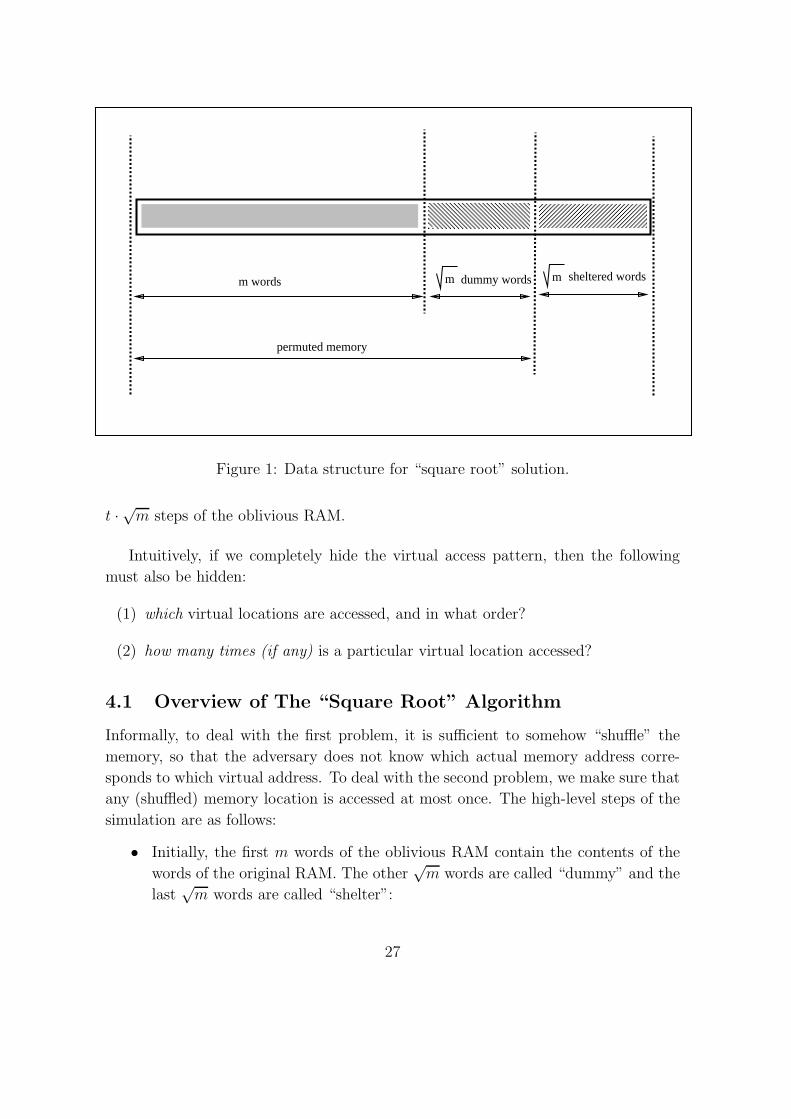
m words m dummy words sheltered wordsm

permuted memory

Figure 1: Data structure for “square root” solution.

t · √m steps of the oblivious RAM.

Intuitively, if we completely hide the virtual access pattern, then the following

must also be hidden:

(1) which virtual locations are accessed, and in what order?

(2) how many times (if any) is a particular virtual location accessed?

4.1 Overview of The “Square Root” Algorithm

Informally, to deal with the first problem, it is sufficient to somehow “shuffle” the

memory, so that the adversary does not know which actual memory address corre-

sponds to which virtual address. To deal with the second problem, we make sure that

any (shuffled) memory location is accessed at most once. The high-level steps of the

simulation are as follows:

• Initially, the first m words of the oblivious RAM contain the contents of the

words of the original RAM. The other√

m words are called “dummy” and the

last√

m words are called “shelter”:

27

• while TRUE do begin:

(1) Randomly permute the contents of locations 1 through m+√

m. That is,

select a permutation π over the integers 1 through m +√

m and relocate

the contents of word i into word π(i) (later, we show how to do this

obliviously)

(2) Simulate√

m memory accesses of the original RAM. During the simu-

lation we maintain the values previously retrieved (during the current

execution of step (2)) in the “sheltered locations” (m +√

m + 1) through

(m + 2√

m) (i.e. locations which are not shuffled, but rather used as a

buffer in which we store values once we retrieve them from the permuted

memory.) A memory access of the original RAM, say an access to word i,

is simulated as follows: first we scan through the “sheltered”√

m words

and check whether the contents of the original i-th word is in one of these

words. If the ith word is not found there then we retrieve it from virtual

word tagged by π(i); else we access the next “dummy word” (i.e. one of

the permuted dummy words π(m+1) through π(m+√

m) which was not

accessed before).

(3) Finally, we return the memory contents to their initial locations.

Before getting to the implementation details of the above steps, we provide some

hints as to why they constitute an oblivious simulation. We are going to show how

to make memory accesses of step (1) fixed and thus independent of the input and

the access pattern of the original RAM. The memory accesses executed in step (2)

are of two types: scanning through all “sheltered” words from the m +√

m + 1-th

to the m + 2√

m-th, and accessing√

m locations which seem to the observer (not

knowing the permutation employed at step (1)) as being chosen at random among

the yet unaccessed words between 1 and m +√

m in the “permuted memory”. It is

easy to see that Step (3) creates no new difficulties, as it can be handled by reversing

the accesses of steps (1) and (2).

4.2 Implementation of the “Square Root” Algorithm

We now turn to details. First, we show how to choose and store a random permutation

over 1, 2, ..., t, using O(log t) storage and a random oracle. The idea is to use

the oracle in order to tag the elements with randomly chosen distinct (with high

probability) integers from a set of tags, denoted Tt. The permutation is obtained by

28

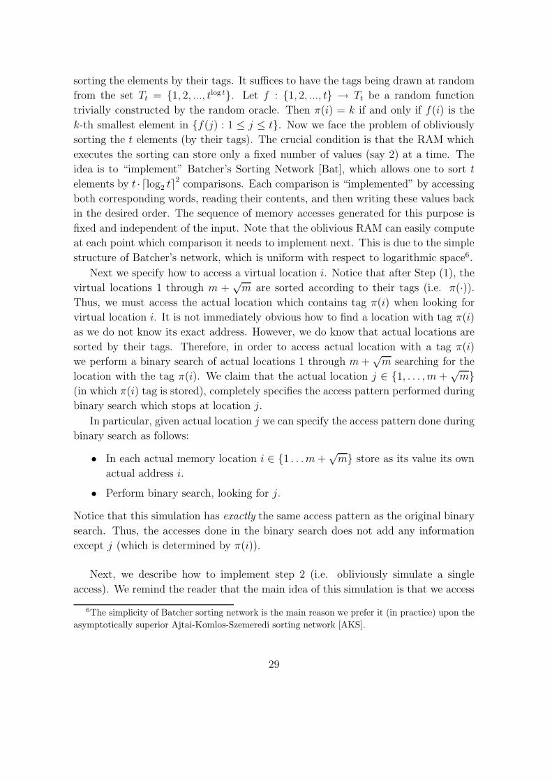
sorting the elements by their tags. It suffices to have the tags being drawn at random

from the set Tt = 1, 2, ..., tlog t. Let f : 1, 2, ..., t → Tt be a random function

trivially constructed by the random oracle. Then π(i) = k if and only if f(i) is the

k-th smallest element in f(j) : 1 ≤ j ≤ t. Now we face the problem of obliviously

sorting the t elements (by their tags). The crucial condition is that the RAM which

executes the sorting can store only a fixed number of values (say 2) at a time. The

idea is to “implement” Batcher’s Sorting Network [Bat], which allows one to sort t

elements by t · ⌈log2 t⌉2 comparisons. Each comparison is “implemented” by accessing

both corresponding words, reading their contents, and then writing these values back

in the desired order. The sequence of memory accesses generated for this purpose is

fixed and independent of the input. Note that the oblivious RAM can easily compute

at each point which comparison it needs to implement next. This is due to the simple

structure of Batcher’s network, which is uniform with respect to logarithmic space6.

Next we specify how to access a virtual location i. Notice that after Step (1), the

virtual locations 1 through m +√

m are sorted according to their tags (i.e. π(·)).Thus, we must access the actual location which contains tag π(i) when looking for

virtual location i. It is not immediately obvious how to find a location with tag π(i)

as we do not know its exact address. However, we do know that actual locations are

sorted by their tags. Therefore, in order to access actual location with a tag π(i)

we perform a binary search of actual locations 1 through m +√

m searching for the

location with the tag π(i). We claim that the actual location j ∈ 1, . . . , m +√

m(in which π(i) tag is stored), completely specifies the access pattern performed during

binary search which stops at location j.

In particular, given actual location j we can specify the access pattern done during

binary search as follows:

• In each actual memory location i ∈ 1 . . .m +√

m store as its value its own

actual address i.

• Perform binary search, looking for j.

Notice that this simulation has exactly the same access pattern as the original binary

search. Thus, the accesses done in the binary search does not add any information

except j (which is determined by π(i)).

Next, we describe how to implement step 2 (i.e. obliviously simulate a single

access). We remind the reader that the main idea of this simulation is that we access

6The simplicity of Batcher sorting network is the main reason we prefer it (in practice) upon the

asymptotically superior Ajtai-Komlos-Szemeredi sorting network [AKS].

29

each virtual memory location in the “permuted memory” only once between each

permutation step. Once we access some virtual location, we keep track of this virtual

location in “sheltered memory” in case we need to access it again. Since “sheltered

memory” (which we constantly scan) has only√

m capacity, we do permutations

with frequency√

m. Thus, throughout step (2), count maintains the number of

single accesses simulated in the current run. The variable count is initially 0 and is

incremented until it reaches√

m. The boolean variable found will record whether

the required value was found in one of the “sheltered”√

m words. When the original

RAM accesses its i-th virtual word, the oblivious RAM proceeds as follows:

(2a) Scans through “sheltered locations” m+√

m+1 to m+2√

m. If the contents of

the original i-th word is in any of these words then the oblivious RAM fetches

it (i.e. stores it in the cpu, and sets found← 1, else set found← 0.

(2b) If found = 1 then the oblivious RAM accesses the word with tag π(m + count)

(which is “dummy”); else the oblivious RAM accesses the word with tag π(i),

retrieves its contents (which is the desired original word i).

(2c) It scans through “sheltered locations” again and writes the (possibly) updated

value of the original i-th word. Increment count by 1.

In order to rearrange the memory, we simply do an oblivious sort of all m + 2√

m

words by the original word location. It should be stressed that only the last accessed

word containing the value of an original is considered as bearing this word. (Note

that during step (2) we can mark words which no longer contain the last accessed

version of an original word.) All other words are considered empty and will be sorted

to the last 2√

m words.

4.3 Analysis of The “Square Root” Algorithm

The reader may easily verify that the sequence of memory accesses of the oblivious

RAM indeed yields no information about the sequence of memory accesses of the

original RAM. This is so, since during sorting, the access-pattern is fixed, and all

other steps are done using a random oracle, and, hence do not reveal any information

about the original work being access in the information-theoretic sense.

It is left to calculate the overhead of the simulation (i.e the ratio of number of

accesses done by the oblivious RAM over the number of original accesses). The

permutation applied after every√

m original accesses causes an overhead of O(m ·log2 m), which amounts to an amortized overhead of O(

√m · log2 m) actions per each

30

original access. In addition, each of the original accesses causes O(√

m) actions to be

taken in step (2). Other actions taken in step (3) are negligible in number. The total

overhead thus amounts to O(√

m · log2 m) actions per instruction (actually, the above

choice of parameters is not optimal. Repermuting the words after every O(√

m·log m)

instructions, yields an overhead of O(√

m · log m) actions per instruction.) Thus, we

have shown that there exist an oblivious simulation of m-size RAMs with O(√

m ·log2 m) overhead.

Our next step makes an exponential improvement: we eliminate a√

m factor in

the simulation and thus reduce overhead from linear to poly-logarithmic. Thus, now

that we developed some tools and intuition, we turn to a much more efficient solution.

5 The Hierarchical Solution

First, we state our main theorem, which is proved in this Section:

Theorem 3 (MAIN RESULT:) For all k ∈ IN, for any RAMk and for all y of length

≤ 2k, any t ≤ 2k steps of the computation of RAMk on y can be obliviously simulated

by probabilistic-RAM ′k+2 log log k with overhead O((log2 t)3). Furthermore, the simulation

is on-line and time-labeled.

5.1 Overview

In this Section we give a high-level description of our algorithm together with some

intuition. The hierarchical solution presented in this Section is a generalization of the

solution presented in the previous Section. One can view the solution of the previous

Section as consisting of two parts: the random shuffling and re-shuffling of the memory

contents every√

m original accesses (steps (1) and (3)), and the simulation of the

original accesses through their randomized locations (step (2)). Substeps (2a) and

(2c) actually simulate a “powerful” RAM in which the CPU can hold up to√

m

values in its local registers at any time: The CPU decides whether it already holds

the required value in its√

m registers (which we call a “buffer”). If the answer is

negative then the CPU fetches the value, else it reaches for a “new” empty cell.

When trying to generalize the solution, we want to decrease the amortized cost of the

random shuffling. The idea, intuitively, is to have buffers of different sizes according

to the frequency with which they are accessed. That is, we will have a small-size

buffer which we frequently access and frequently shuffle. We will have bigger and

bigger buffers which are not as frequently accessed and hence will not have to be

31

shuffled as frequently, striking a balance in the (amortized) cost. Hence, intuitively

our approach, is to design a solution using a “powerful” RAM with CPU which can

hold a constant fraction of the original memory, and then simulate such a RAM by

a smaller RAMs in a recursive fashion. Thus, we introduce a hierarchy of buffers

of different sizes, where essentially we are going to “shuffle” buffers with frequency

roughly proportional to their sizes.

For exposition purposes, we again make (another) simplifying assumption about

the possible access pattern and first present a solution for this simpler problem.

Remark: At first reading, it will not be clear why we select this particular solution

for the simplified problem. The reason, however, will become obvious, once we show

how to extend it to the general case.

5.2 The Restricted Problem

Suppose somebody guarantees to us that every memory location in a contiguous block

A of memory of length n is going to be read once and only once (we assume that

each memory location Vi (V stands for “virtual”) in A contains a value Xi. Thus,

A = ((V1,X1), . . . , (Vn,Xn)).) In this Section we consider the problem of hiding the

access pattern into A. That is, we hide the order (i.e. the permutation!) in which

words in A are examined. Instead of taking the simple approach of the previous

Section, we introduce a new data-structure, which will prove to be useful for our

general problem. In particular, instead of just permuting memory contents, we create

a hash-table with 4n “buckets”, numbered from 1 to 4n, where each bucket will

contain O(log n) words (as indicated on the figure of the restricted problem).

We are going to map virtual memory addresses to keys in the hash table, using

the random oracle to compute our hash function. That is, we define our hash function

h(V) to be F (V) mod 4n. (Recall that we denote by F (i) a call to a random oracle

on input i.) The pre-processing step works as follows:

(1) Allocate a new block of memory of size 4n · O(log n) words. In this block, we

call each consecutive sub-block of size O(log n) a bucket , and we number our

buckets from 1 to 4n.

(2) Pick a random index s. Given s, we define a hash-function hs(·) to map any

address V in A to an address hs(V) which we define as hs(V) = F (sV) mod 4n.

(3) (“Oblivious hash”): For i from 1 to n do: obliviously store a pair (Vi,Xi). into a

bucket hs(Vi) (i.e. into the first available word in a bucket hs(Vi)). That is, store

32

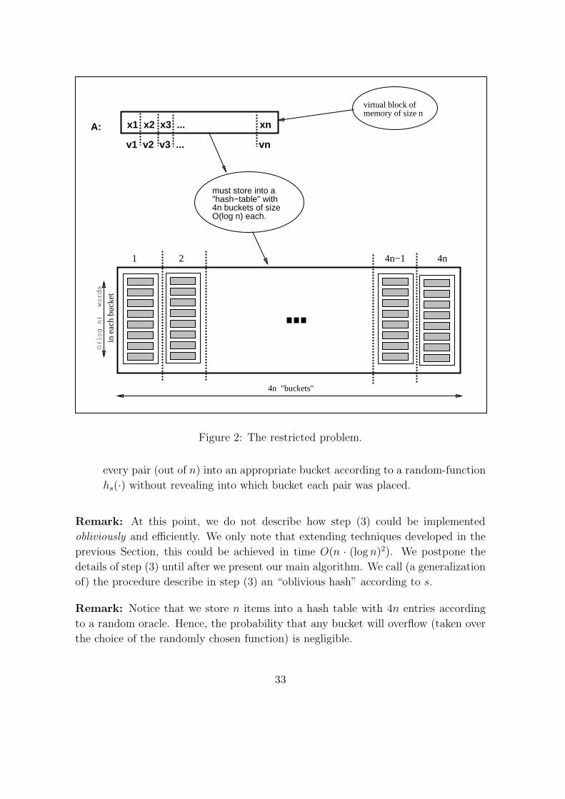
O(lo

g n

) w

ord

s

4n "buckets"

in e

ach

buck

et

1 2 4n−1 4n

A: x1 x2 x3 ... xn

v1 v2 v3 ... vn

virtual block ofmemory of size n

must store into a"hash−table" with4n buckets of sizeO(log n) each.

Figure 2: The restricted problem.

every pair (out of n) into an appropriate bucket according to a random-function

hs(·) without revealing into which bucket each pair was placed.

Remark: At this point, we do not describe how step (3) could be implemented

obliviously and efficiently. We only note that extending techniques developed in the

previous Section, this could be achieved in time O(n · (log n)2). We postpone the

details of step (3) until after we present our main algorithm. We call (a generalization

of) the procedure describe in step (3) an “oblivious hash” according to s.

Remark: Notice that we store n items into a hash table with 4n entries according

to a random oracle. Hence, the probability that any bucket will overflow (taken over

the choice of the randomly chosen function) is negligible.

33

Recall that we are dealing with the restricted problem, where we assume that our

access pattern is a permutation. After the pre-processing step, we can easily hide the

access pattern, utilizing the assumption that every virtual memory location V in A

is referenced once and only once. To do so, when looking for a value stored under a

virtual address V we completely scan bucket h(V) looking for a tuple (V, ·). Notice

that any two distinct virtual memory locations are assigned independent buckets and

every virtual memory location (by our assumption) is accessed at most once. Thus,

the (actual memory) access pattern (i.e. bucket-access pattern) is independent of the

virtual memory access pattern. Moreover, the probability of an overflow is negligible.

Claim 1 Assume that every element in a block A of memory of length n is accessed

once and only once. Then there exists an (off-line) oblivious simulation with Θ((log n)2)

overhead.

Remark: We emphasize a crucial point of the above solution: our procedure is

allowed to access the same bucket more than once. In fact, it will do so when collisions

occur. Notice, however, that the distribution is the same as if we select (for n times)

one of the 4n buckets uniformly at random and sequentially scan it.

5.3 The Algorithm

In this Section we show how to hide the access pattern with just polylog(t) slowdown in

the running time. We waive all the previous restrictions, and allow multiple accesses

to the same location and do not rely on the a-priori knowledge of the total (RAM)

memory size.

Instead of a single hash-table introduced in the previous Section, we use several

hash-tables of different sizes. With each hash-table, we associate a different hash-

function, i.g. a different index si. We call these hash-tables “buffers”. We number

them from 1 to N and refer to the i’th “level” buffer when we talk about buffer

number i, 1 ≤ i ≤ N (see “hierarchical data-structure” figure.) We “obliviously

hash” contents of buffers at different intervals, according to their sizes (for smaller

buffers we do so more often than for bigger ones). The idea is to ensure that for

each buffer, no element in that buffer is accessed more than once in between two

consecutive “oblivious hashes”, thus reducing the general problem to the simplified

problem of the previous Section.

Let t be the current length of the access sequence, (i.e., the current running time

of the program which is being simulated). Note that initially, t is equal to input

34

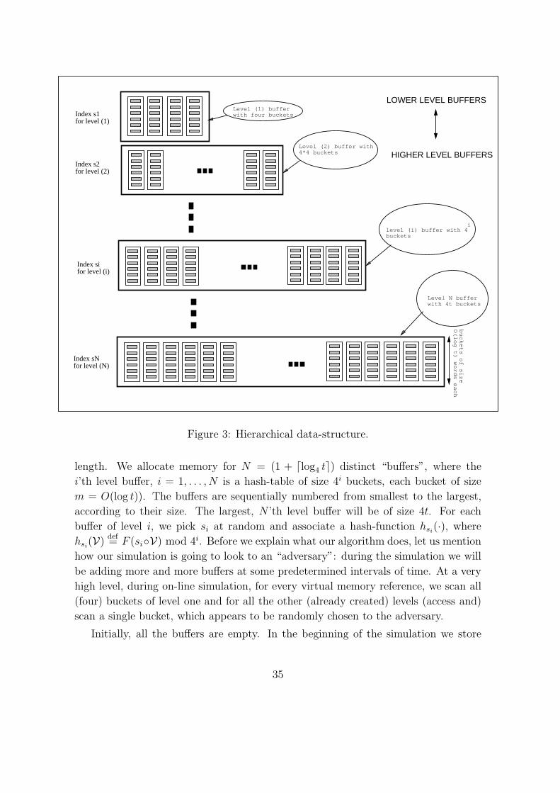
Level (1) bufferwith four buckets

level (i) buffer with 4buckets

i

Level (2) buffer with4*4 buckets

Level N bufferwith 4t buckets

LOWER LEVEL BUFFERS

HIGHER LEVEL BUFFERS

bu

ckets o

f sizeO

(log

t) wo

rds e

ach

Index s1for level (1)

Index s2for level (2)

Index sifor level (i)

Index sNfor level (N)

Figure 3: Hierarchical data-structure.

length. We allocate memory for N = (1 + ⌈log4 t⌉) distinct “buffers”, where the

i’th level buffer, i = 1, . . . , N is a hash-table of size 4i buckets, each bucket of size

m = O(log t)). The buffers are sequentially numbered from smallest to the largest,

according to their size. The largest, N ’th level buffer will be of size 4t. For each

buffer of level i, we pick si at random and associate a hash-function hsi(·), where

hsi(V)

def= F (siV) mod 4i. Before we explain what our algorithm does, let us mention

how our simulation is going to look to an “adversary”: during the simulation we will

be adding more and more buffers at some predetermined intervals of time. At a very

high level, during on-line simulation, for every virtual memory reference, we scan all

(four) buckets of level one and for all the other (already created) levels (access and)

scan a single bucket, which appears to be randomly chosen to the adversary.

Initially, all the buffers are empty. In the beginning of the simulation we store

35

(i.e. “obliviously hash”) the program and the input into the biggest, N ’th level

buffer according to the value of sN and answers of the random oracle. During on-line

simulation, when we need to access virtual memory reference V, we first completely

scan the level 1 buffer, looking for it. If we have not found (V,X ) at level 1, then we

scan bucket hs2(V) of level 2. If we have not found it there, we scan hs3

(V) if level

3, etc. Say we find the virtual memory reference we been looking for at some level

(j), then for all the higher (i.e., bigger) levels, we access and scan a randomly chosen

bucket. At the end, we store the found virtual “address-value” pair (V,X ) at the

level 1 buffer. (We stress that we store in the level 1 buffer only the “address-value”

pair we been looking for, and not the entire bucket in which we have found it. )

In summary, here is how the value of the virtual location V is retrieved:

• Set boolean variable found to false and change it to “true” only when contents

of virtual location V is found, as specified below.

(1) Sequentially scan the level 1 buffer, looking for (V,X ); (we remark that once

found, the cpu keeps (V,X ) pair in its work tape (i.e. in its registers) until

Step (3) below.)

(2) For i from 2 to n do:

– Retrieve the i’th level index si (of the current hash function associated

with buffer level i) and compute hsi(V).

– IF virtual location V has already been found THEN access a “random”

location. Namely, pick a random integer r between 1 and 4i and scan

bucket r.

– ELSE scan bucket number hsi(V), looking for a tuple (V,X ). If found,

set found to true, and copy (V,X ) onto cpu work tape. (We remark

that we scan entire bucket even if we already found the tuple, and for

each element of the bucket, we perform an access pattern as if we copy

it into cpu work tape)

(3) Copy (V,X ) from cpu work tape into the first empty bucket of the level 1

buffer.

Note that in the above description, the data is is always “moved up” to the level

1 buffer. Thus, after four accesses, the level 1 buffer may become full. To avoid

potential “overflow” we must “move” contents of the first level buffer to the second

36

level buffer. Then (at longer intervals) we must move contents of the second level

buffer to the third level buffer, etc. When we “move” contents of buffer level i to

buffer level i + 1, (we do this every 4i−1 retrieves) we “obliviously hash” the contents

of buffer level i and the contents of buffer level i + 1 to the buffer i + 1 according to

a new, randomly chosen index s′i+1. Thus, every time a buffer at level i becomes at

most quarter-full7 (i.e. has the number of stored virtual memory references equal to

at most a quarter of the number of the buckets) we empty it into the higher level. If

the higher level does not yet exist, we allocate it.

Remark: Notice that at round 4i, the total number of entries in the first i buffers is

at most 4i, and hence merging their contents into the ith buffer (of size 4i+1 buckets)

can use up only a quarter (of the total number of buckets) of the entries.

Remark: Note that when we move contents of lower level buffer into the larger

buffer, we pick a new hash-function and put into the bigger buffer the contents of

the smaller buffer and the contents of the bigger buffer according to this new hash

function. Thus, the collisions which occurred in the smaller buffer do not influence

collisions which may occur in the bigger buffer. That is, collisions do not accumulate.

Remark: Note that we do not need to know a-priori the length of the request

sequence. Instead, we do an adaptive simulation, starting with twice the size of the

input and adding more memory “as needed”, (but obliviously of the real access.)

That is, after t steps we use O(t · (log t)2) memory. Notice that this does not reveal

the rate at which the memory is actually used up by the program.

5.4 Obliviousness of Access Pattern

From our examination of the restricted problem (see Section ??), we know that as

long as we look for any memory reference at most once, the choice of the hash-bucket

accessed appears completely random to the adversary. Notice that there may be

“collisions” (i.e. we scan the same bucket more the once), but since different memory

locations are assigned independent buckets, the choice of a bucket (for any memory

reference unaccessed-before) appears random to the adversary.

7Notice that if we access the same actual location, instead of different actual locations, then

buffers do not fill-up. , The algorithm, never-the-less, moves contents of buffers at regular intervals

of time, even though they may even be empty. That is, we move the contents of the buffers, which

are at worst quarter-full. Intuitively, this assures that the buckets do not overflow with overwhelming

probability.

37

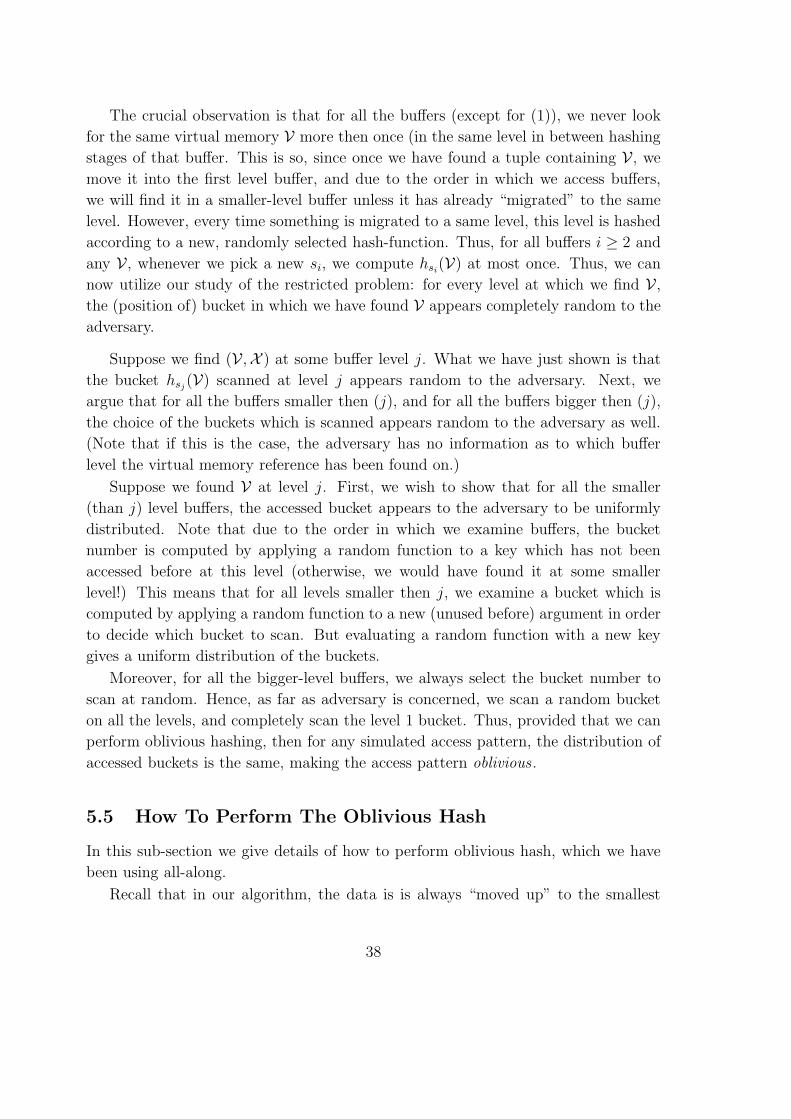
The crucial observation is that for all the buffers (except for (1)), we never look

for the same virtual memory V more then once (in the same level in between hashing

stages of that buffer. This is so, since once we have found a tuple containing V, we

move it into the first level buffer, and due to the order in which we access buffers,

we will find it in a smaller-level buffer unless it has already “migrated” to the same

level. However, every time something is migrated to a same level, this level is hashed

according to a new, randomly selected hash-function. Thus, for all buffers i ≥ 2 and

any V, whenever we pick a new si, we compute hsi(V) at most once. Thus, we can

now utilize our study of the restricted problem: for every level at which we find V,

the (position of) bucket in which we have found V appears completely random to the

adversary.

Suppose we find (V,X ) at some buffer level j. What we have just shown is that

the bucket hsj(V) scanned at level j appears random to the adversary. Next, we

argue that for all the buffers smaller then (j), and for all the buffers bigger then (j),

the choice of the buckets which is scanned appears random to the adversary as well.

(Note that if this is the case, the adversary has no information as to which buffer

level the virtual memory reference has been found on.)

Suppose we found V at level j. First, we wish to show that for all the smaller

(than j) level buffers, the accessed bucket appears to the adversary to be uniformly

distributed. Note that due to the order in which we examine buffers, the bucket

number is computed by applying a random function to a key which has not been

accessed before at this level (otherwise, we would have found it at some smaller

level!) This means that for all levels smaller then j, we examine a bucket which is

computed by applying a random function to a new (unused before) argument in order

to decide which bucket to scan. But evaluating a random function with a new key

gives a uniform distribution of the buckets.

Moreover, for all the bigger-level buffers, we always select the bucket number to

scan at random. Hence, as far as adversary is concerned, we scan a random bucket

on all the levels, and completely scan the level 1 bucket. Thus, provided that we can

perform oblivious hashing, then for any simulated access pattern, the distribution of

accessed buckets is the same, making the access pattern oblivious .

5.5 How To Perform The Oblivious Hash

In this sub-section we give details of how to perform oblivious hash, which we have

been using all-along.

Recall that in our algorithm, the data is is always “moved up” to the smallest

38

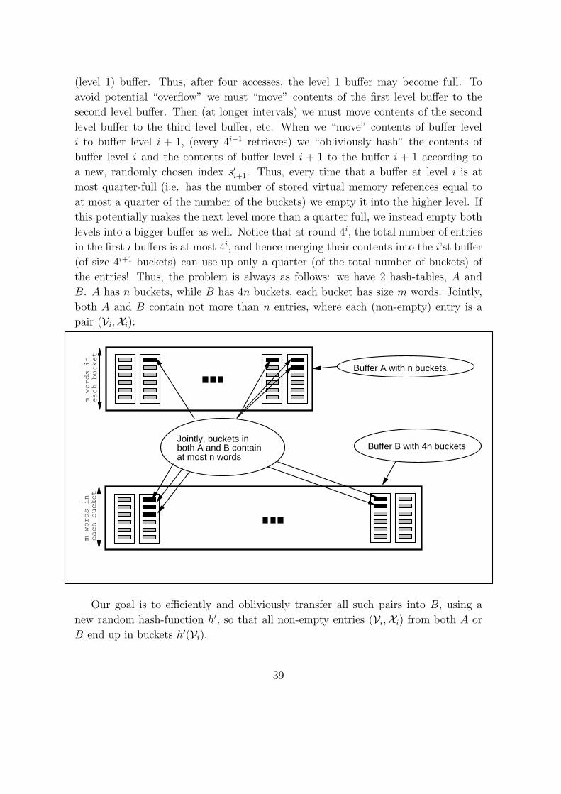
(level 1) buffer. Thus, after four accesses, the level 1 buffer may become full. To

avoid potential “overflow” we must “move” contents of the first level buffer to the

second level buffer. Then (at longer intervals) we must move contents of the second

level buffer to the third level buffer, etc. When we “move” contents of buffer level

i to buffer level i + 1, (every 4i−1 retrieves) we “obliviously hash” the contents of

buffer level i and the contents of buffer level i + 1 to the buffer i + 1 according to

a new, randomly chosen index s′i+1. Thus, every time that a buffer at level i is at

most quarter-full (i.e. has the number of stored virtual memory references equal to

at most a quarter of the number of the buckets) we empty it into the higher level. If

this potentially makes the next level more than a quarter full, we instead empty both

levels into a bigger buffer as well. Notice that at round 4i, the total number of entries

in the first i buffers is at most 4i, and hence merging their contents into the i’st buffer

(of size 4i+1 buckets) can use-up only a quarter (of the total number of buckets) of

the entries! Thus, the problem is always as follows: we have 2 hash-tables, A and

B. A has n buckets, while B has 4n buckets, each bucket has size m words. Jointly,

both A and B contain not more than n entries, where each (non-empty) entry is a

pair (Vi,Xi):

Buffer A with n buckets.

Buffer B with 4n buckets

m w

ord

s in

e

ach

bu

cke

tm

wo

rds

in

ea

ch b

uck

et

Jointly, buckets inboth A and B containat most n words

Our goal is to efficiently and obliviously transfer all such pairs into B, using a

new random hash-function h′, so that all non-empty entries (Vi,Xi) from both A or

B end up in buckets h′(Vi).

39

The requirement of making this transfer oblivious demands the access pattern of

our algorithm to be independent (among all other things) of the number of entries in

each (old or new) bucket. In particular, the issue is the following. What we know is

how to obliviously sort n distinct elements into n cells, whereas what we need to do

now is obliviously hash n not necessarily distinct elements into n cells. Furthermore,

the elements will be independently and uniformly assigned a cell number and they

should be obliviously put into this cell. Note that it is expected that a constant

fraction of the cells are assigned no element, a constant fraction are assigned one

element, a (smaller) constant fraction are assigned two elements, and it is likely that

there is a cell assigned log2 n elements. The hashing should be performed so that, in

particular, the number of elements in each target cell is kept secret.

Recall that in the “square root” solution we assigned “tags” to the elements and

then sorted according to these “tags”. Here, the “tag” indicates the specific bucket

in which the the elements (i.e. virtual words) must be put. Notice that we want

to place up to n words into designated random 4n buckets (of B), where each word

is assigned a destination “tag” which corresponds to the bucket number into which

this word must be obliviously put. This can not be obtained by just obliviously

sorting these words by their tags since the words do not necessarily get unique tags

(and in fact, with high probability collisions do occur, as indicated above.) Notice

that if the tags were indeed unique then there would be no issue, as we could of

just apply the approach developed in our “square root” solution for the case of the

permutation. That is, while we already know how to achieve oblivious sorting ‘q(i.e,

in the square-root solution), it is not clear that the ability to obliviously sort will allow

us to obliviously put elements in the right buckets (instead of just sorting them). The

problem, intuitively, is that even after the valid entries are sorted by their new keys,

it is not clear how they can be efficiently and obliviously put into their appropriate

buckets. Thus, what we wish to do is to first somehow initialize all the buckets to have

the correct contents, and then obliviously put these buckets into the right position.

In fact, one of the things we are going to do is to first sort valid entries by their

new keys. Notice that since collisions do occur, there will be many entries with the

same key. Next, we must put the entries in the appropriate buckets. The way we are

going to achieve this is to use many applications of “oblivious sorting” using different

“granularities” of elements which are sorted — the idea, in essence, is to reduce the

above problem to the already known case of obliviously sorting a permutation. In

particular, we are going to to use “oblivious sorting” for the following purposes:

(a) sorting elements within a bucket: we mark all the “empty” entries as zero and

all the “full” entries as one and then perform an oblivious sort. As a result,

40

all the “empty” and “full” entries are grouped together.

(b) moving elements within two buckets: Again, the idea is to mark all the empty

elements in both buckets as zero and all the non-empty elements as one and

then obliviously sort. Since we are going to be guaranteed (with high prob-

ability) that the number of non-empty entries will be less then the size of a

bucket, we essentially manage to “move” all the non-empty entries into one of

the buckets, while keeping the access pattern completely oblivious.

(c) sorting buckets as individual elements: we can now put buckets (as individual

elements) according to their numbering, provided that all buckets are repre-

sented.

In order to make sure that we are dealing with all the buckets, (i.e. that we are

dealing with the permutation), we introduce a “dummy” entry for each bucket. This

way, we are guaranteed that there is at least one item that we must put into each

bucket. Then we sort all the entries by their keys. Then we put the designated words

(and “dummy” entries) into buckets according to their tags (Step 5) using oblivious

sorting (sorting two buckets at a time as in (b)) and then put buckets into their

appropriate places obliviously sorting then as in in (c) above and then just copying

them into B in the open (as it does not release any information as this point). Now

we turn to a detailed description. The steps of oblivious hash algorithm are as follows:

1. Create a new hash-table C, of size 5n buckets, and copy contents of A and

B into C, bucket by bucket (i.e. treating each bucket as indivisible block of

memory of size m words.)

bucket 1 bucket 5n

1 2 3 4 5nm−1 5nm1

C:

Remark: the intuition here is that we put all the data from A and B to a

“temporary” bucket C, in which we “garbage-collect” all the empty words in an

oblivious manner. In order to do so, we essentially “mark” all the empty words

with “0”, all the non-empty words with positive numbers and then perform

41

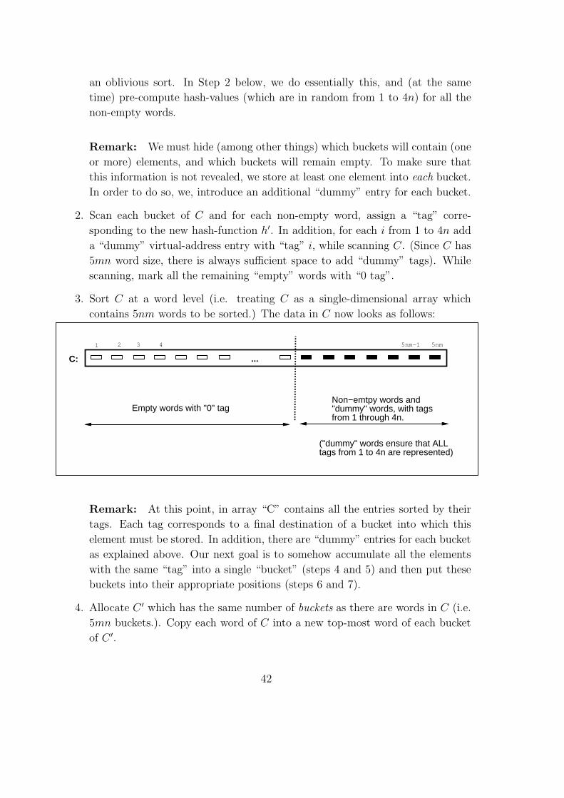
an oblivious sort. In Step 2 below, we do essentially this, and (at the same

time) pre-compute hash-values (which are in random from 1 to 4n) for all the

non-empty words.

Remark: We must hide (among other things) which buckets will contain (one

or more) elements, and which buckets will remain empty. To make sure that

this information is not revealed, we store at least one element into each bucket.

In order to do so, we, introduce an additional “dummy” entry for each bucket.

2. Scan each bucket of C and for each non-empty word, assign a “tag” corre-

sponding to the new hash-function h′. In addition, for each i from 1 to 4n add

a “dummy” virtual-address entry with “tag” i, while scanning C. (Since C has

5mn word size, there is always sufficient space to add “dummy” tags). While

scanning, mark all the remaining “empty” words with “0 tag”.

3. Sort C at a word level (i.e. treating C as a single-dimensional array which

contains 5nm words to be sorted.) The data in C now looks as follows:

1 2 3 4 5nm−1 5nm1

C: ...

Non−emtpy words and"dummy" words, with tagsfrom 1 through 4n.

("dummy" words ensure that ALLtags from 1 to 4n are represented)

Empty words with "0" tag

Remark: At this point, in array “C” contains all the entries sorted by their

tags. Each tag corresponds to a final destination of a bucket into which this

element must be stored. In addition, there are “dummy” entries for each bucket

as explained above. Our next goal is to somehow accumulate all the elements

with the same “tag” into a single “bucket” (steps 4 and 5) and then put these

buckets into their appropriate positions (steps 6 and 7).

4. Allocate C ′ which has the same number of buckets as there are words in C (i.e.

5mn buckets.). Copy each word of C into a new top-most word of each bucket

of C ′.

42

1 2 3 4 5nm−1 5nm1

1 2 3 4 5nm−1 5nm1

Going from C to C’

Remark: At step 4 we created a correct data-structure to accumulate all the

entries with the same “tag” into a single bucket of C ′, which we can now do in

step 5 as follows:

5. Scan C ′ buckets left to right, performing oblivious sort between words of every

two adjacent buckets, and in the process, “accumulating” all the data with the

same “tag” into unique buckets of C ′ (Note that due to “dummy” entries, all

“tags” from 1 to 4n are represented.) That is for every two pairs of buckets,

if they contain different tags, execute oblivious hash but do nothing. If they

have the same tags, treat all non-empty entries as 1’s and all empty entries as

0’s and perform oblivious hash. This way, all the empty entries are left in the

first bucket, while all the non-empty entries are moved to the next bucket, as

explained in step (c) above.

43

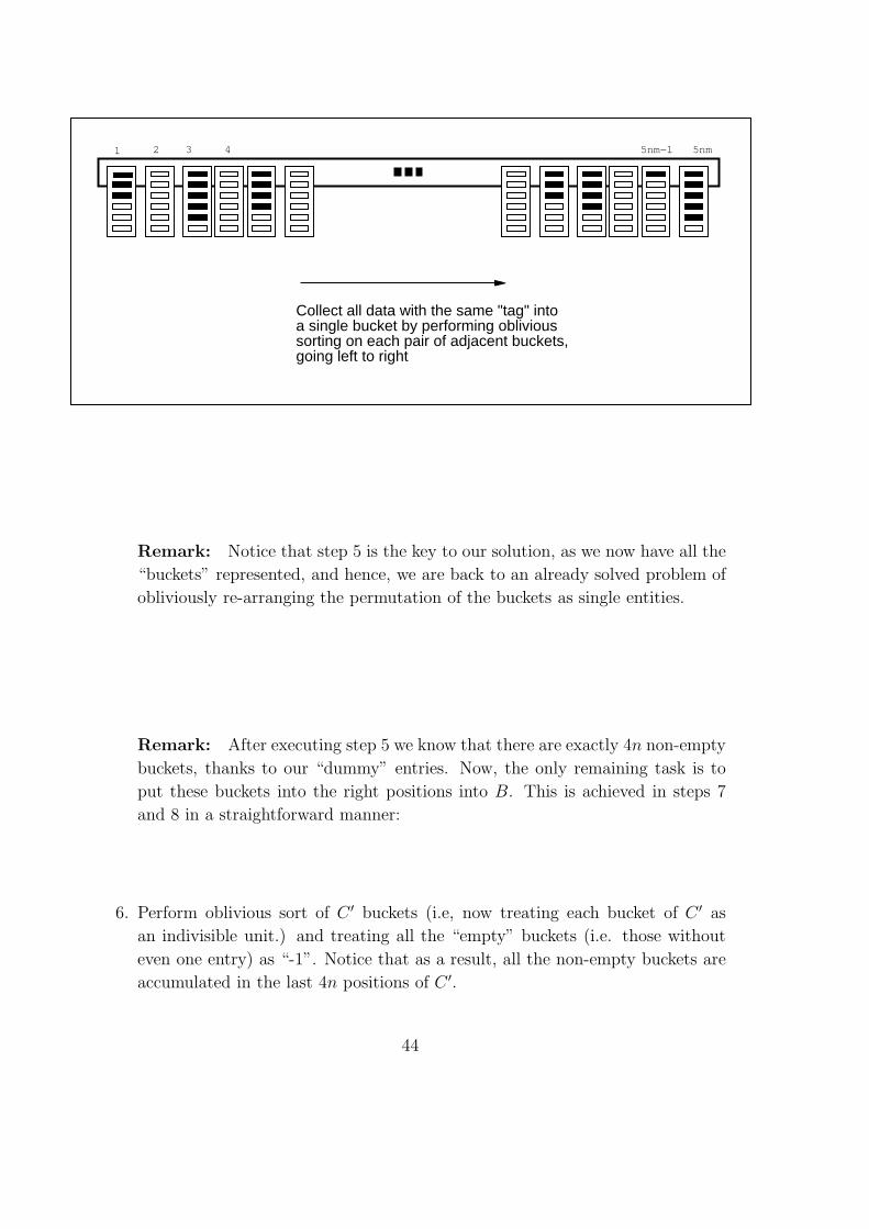
1 2 3 4 5nm−1 5nm1

Collect all data with the same "tag" intoa single bucket by performing oblivious sorting on each pair of adjacent buckets,going left to right

Remark: Notice that step 5 is the key to our solution, as we now have all the

“buckets” represented, and hence, we are back to an already solved problem of

obliviously re-arranging the permutation of the buckets as single entities.

Remark: After executing step 5 we know that there are exactly 4n non-empty

buckets, thanks to our “dummy” entries. Now, the only remaining task is to

put these buckets into the right positions into B. This is achieved in steps 7

and 8 in a straightforward manner:

6. Perform oblivious sort of C ′ buckets (i.e, now treating each bucket of C ′ as

an indivisible unit.) and treating all the “empty” buckets (i.e. those without

even one entry) as “-1”. Notice that as a result, all the non-empty buckets are

accumulated in the last 4n positions of C ′.

44

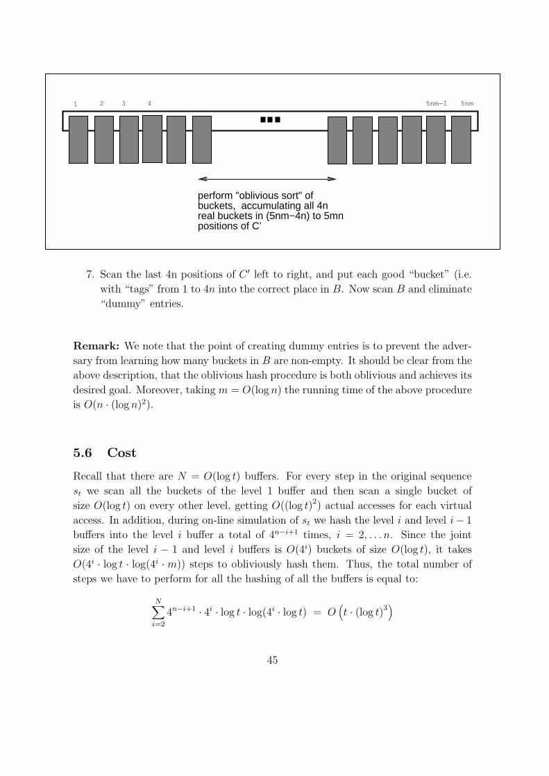
1 2 3 4 5nm−1 5nm1

perform "oblivious sort" ofbuckets, accumulating all 4nreal buckets in (5nm−4n) to 5mnpositions of C’

7. Scan the last 4n positions of C ′ left to right, and put each good “bucket” (i.e.

with “tags” from 1 to 4n into the correct place in B. Now scan B and eliminate

“dummy” entries.

Remark: We note that the point of creating dummy entries is to prevent the adver-

sary from learning how many buckets in B are non-empty. It should be clear from the

above description, that the oblivious hash procedure is both oblivious and achieves its

desired goal. Moreover, taking m = O(log n) the running time of the above procedure

is O(n · (log n)2).

5.6 Cost

Recall that there are N = O(log t) buffers. For every step in the original sequence

st we scan all the buckets of the level 1 buffer and then scan a single bucket of

size O(log t) on every other level, getting O((log t)2) actual accesses for each virtual

access. In addition, during on-line simulation of st we hash the level i and level i− 1

buffers into the level i buffer a total of 4n−i+1 times, i = 2, . . . n. Since the joint

size of the level i − 1 and level i buffers is O(4i) buckets of size O(log t), it takes

O(4i · log t · log(4i · m)) steps to obliviously hash them. Thus, the total number of

steps we have to perform for all the hashing of all the buffers is equal to:

N∑

i=2

4n−i+1 · 4i · log t · log(4i · log t) = O(t · (log t)3

)

45

Therefore, we have an amortized poly-logarithmic (i.e. O((log t)3)) overhead of hiding

the access pattern (with a negligible probability of an overflow8).

Remark: Our negligible probability of error can be substituted to expected (polylog)

running time by requiring the running time to be an expected polylog overhead, and

hashing whenever overflow occurs.

Remark: Notice that there is a trade-off between the size of the cpu and the overhead

of the simulation. That is, given more (“protected” from the adversary) memory in

the cpu, we can always speed-up our simulation.

5.7 Making Hierarchical Simulation Time-Labeled

Recall that we need to make our simulation time-labeled in order to prevent an adver-

sary from substituting values previously stored in the same actual location. Before

we present our solution we make a crucial observation:

Lemma 1 During our (hierarchical) simulation, for all buffers of levels bigger than one

we do not change the contents of these buffers except by oblivious hashing.

Proof: Notice that we do not have to modify the bucket when we scan it. Mod-

ifications happen only during re-hashing (and on buffer level (1)). Recall that this

is possible since whenever we wish to “change” some location, we always move it to

the first level buffer, and hence, can change it there. Hence, we do not “touch” the

bucket where we have found it.

Due to the above lemma, our simulation is trivially time-labeled, as we touch each

level with a fixed frequency which depends only on the size of that level and total

elapsed time of the simulation. This completes the proof of theorem 3.

5.8 Software protection

We can now combine theorem 3 and 2 to establish that:

Theorem 4 SOFTWARE PROTECTION (information-theoretic case): There

exists a software-protecting compiler C such that for any probabilistic-RAM C protects

software against tampering adversaries with overhead O((log2)3).

8We throw n balls into 4n boxes and measure the probability that any box contains more then

c log n balls, which corresponds to an overflow. The probability of this event can be easily seen to

be neglibible, where by negligible we mean asymptotically less then 1

nO(1) .

46

The above theorem holds in the information-theoretic sense on a probabilistic-

RAM (which uses a random oracle.) As noted in the introduction, instead of random

oracle we can use pseudo-random functions [GGM], and state a practical analogue of

the above theorem. That is, assuming the existence of a strong one-way function, the

above algorithm can be implemented in practice using O(t · (log2 t)3 · kc) steps. Thus

the above overhead is (log2 t)3 ·kc. We claim that if we substitute a random oracle by

a pseudo-random one, with an appropriate security parameter, then (log2 t)3 < kc and

thus the overhead is just O(kc). This is so since k is a security parameter, and t is the

running time. Hence, However, the security parameter k implies that 2k is infeasible.

Thus, if we consider only poly-time computations, (t) << 2k, and (log2 t)3 < kc for

c ≥ 3. Thus, we can state a practical analogue of Theorem 4 as follows:

Theorem 5 SOFTWARE PROTECTION (polynomial case): Suppose one-

way functions exist, with k a security parameter of a strong one-way function. Then there

exists a software-protecting compiler C secure against all polynomial-time adversaries with

compilation overhead kO(1).

Proof : Analogous to the information-theoretic case, but substituting the random

oracle by a pseudo-random one. That is, we initialze a cpu with a seed to a random

oracle, and ougmment our cpu with [GGM] speudo-random function hardware. Every

time there is a call to a random oracle, we make a call this this hardware stored in

the cpu. The rest of the algorithm is equivalent to the information-theoretic case.

6 A Lower Bound

Theorem 6 Every oblivious simulation of ram on input y by probabilistic-ram must

make at least (max|y|, Ω(t · log t) accesses in order to simulate t steps.

Proof : The task of simulating ram on an oblivious RAM can be modeled by the

following game between three players:

• the cpu player who can hold at one time at most c “balls” and has access to

random function f .

• the program request sequence: (r1, . . . , rt) of length t.

• an observer.

47

The player is allowed at any point in time to inspect the entire program request

sequence. The game takes place on a memory consisting of m cells, each capable of

storing a single ball. The balls are numbered, from 1 to m. Initially, the ith cell

contains ball number i, for 1 ≤ i ≤ m. (By m we denote the maximal amount of

memory that ram can use on input y and t steps of the execution. Notice that m is

at most max|y|, t.)

The game proceeds for t rounds. In each round j, the program request sequence

secretly specifies to the player a request rj which is a ball number from 1 to m (say

i). The goal of the player is to hold the ball rj but in such a way that the observer

does not know the value of rj. That is, the obliviousness condition requires that the

observer can learn nothing about the sequence of requests initiated by the program

from the sequence of addresses accessed by the player. We note that the program

request sequence is collaborating with neither the player nor observer.

In order to achieve the above goal, the player “answers” by a sequence of exchanges

of balls that he currently has and balls stored in memory (or just touches of balls

stored in memory). The current round ends when the player holds ball i. The observer

sees the sequence of (memory) addresses accessed, but does not see any of the ball

numbers nor whether the balls in memory are just touched or exchanged.

Consider a probabilistic mapping of t-element long request sequence (i.e. the re-

quest made by the program) into a pair of two q-element sequences determining the

behavior of the CPU player. The first sequence Vq describes the visible access pattern

while the second sequence Hq describes the hidden sequence of actions (elements of

EXCHANGE(l)1≤l≤c,

DROP(l)1≤l≤c, TAKE(l)1≤l≤c, DO-NOTHING). Hence, in response to request se-

quence (r1, ..., rt) and access to random function f , the player conducts actions

(v1, h1), . . . , (vq, hq) where vi is a cell number from Vq and hi denotes above men-

tioned 3c + 1 actions from Hq (i.e., whether the player “takes (a ball from the cell)”,

“drops (a ball into it)” or “keeps (the balls he holds)”.

We can now specify exactly the notion of “rounds”: we say that a sequence

of actions (v1, h1), ..., (vq, hq) satisfies the request sequence r1, ..., rt if there exists

a sequence i1, ..., it (i.e., when rounds are “finished”) so that, for every (round) j

(1 ≤ j ≤ t), after actions (v1, h1), ..., (vij , hij) the player holds ball rj (i.e., request to

get ball rj is satisfied). Note that this definition does not depend on the function f

(which might have been used to determine the action sequence).

48

Note that a fixed sequence of player actions (v1, h1), ..., (vq, hq) may satisfy at

most cq program request sequences, as after each step the player holds at most c balls.

Moreover, for a fixed Vq there are (3c + 1)q possible request sequences. Therefore,

each Vq of length q may satisfy at most cq · (3c + 1)q request sequences. By the

obliviousness condition, the Vq sequence should be statistically independent of the

particular request sequence (except for its length). But there are mt requests, calling

for at least this number of hidden actions. Thus, for any constant c (which corresponds

to the oblivious ram that has probabilistic cpu with c registers) it must be the case

that q > t · Ω(log m).

Remark: The above proof does not use the fact that the simulation needs to be done

on-line. That is, the above lower bound holds even if the simulation is performed with

the entire program request sequence given to the oblivious ram before the simulation

begins!

7 Concluding Remarks

Summarizing, we provided theoretical treatment of software protection in terms of

formalizing what the problem is, and establishing poly-logarithmic upper bound and

logarithmic lower bound.

Moreover, we have established the analog of Pippenger and Fisher result [PF] for

random-access machines, despite the fact that random-access machines can access its

memory in an arbitrary manner, whereas the result of [PF] relies on the fact that

single-tape Turing machine memory-access is severely limited.

On a practical side, we have presented a compiler which translates RAM-programs

to equivalent programs which defeat attempts to learn anything about the program

by executing it. The translation was carried-out on the instruction level: namely,

we have replaced the memory access of each instruction by a sequence of redundant

memory accesses. Clearly, all statements and results appearing above, apply to any

other level of execution granularity. For example, on the “paging” level this would

mean dealing with “get page” and “store page” as atomic access instructions, and

substituting single ”page access” by a sequence of “page accesses”. In general, we

have provided a mechanism for obliviously accessing a large number of unprotected

sites when using a single protected site. This has several applications.

One possible application of our work is protection of traffic-patterns in a dis-

tributed database. In this application we deal with a distributed database in which

no user can hold at one time more than a small part of the database, and in which

49

a polynomial-time adversary can monitor all communication lines. Encryption hides

the contents of the messages, but does not hide which communication lines are used.

Thus, indirectly, some information about the database is revealed to an adversary.

For example, an adversary can learn which part of the database is most useful (i.e.,

most frequently read and updated), and which part of the database is most useful to

a particular user. How can users hide the access sequence without sending too many

additional messages? It can be shown that a solution to the “obliviously accessed

data base” problem reduces to simulation of arbitrary RAMs by oblivious RAMs.

We note that further work in this direction, dealing with a more powerful adversary

was addressed in [SR].

Another application of our technique is for data-structure checking [B, BK, BEGKN],

where assuming that a data-structure has small reliable memory we can guarantee

that it was not modified by an adversary.

References

[AHU] Aho, A.V., J.E. Hopcroft, and J.D. Ullman, “The Design and Analysis of

Computer Algorithms” Addison-Wesley Publ. Co., 1974

[AKS] Ajtai, M., J. Komlos, and E. Szemeredi “An O(n · log n) Sorting Network”

STOC 83.

[ACGS] Alexi, W., B Chor, O Goldreich, and C.P Schnorr, “RSA and Rabin Func-

tions: Certain Parts Are As Hard As The Whole”, SIAM Jour on Comput-

ing, Extended Abstract in Proc 25th FOCS, 1984.

[Bat] Batcher, K. “Sorting Networks and their Applications” AFIPS Spring Joint

Computer Conference 32, 1968, pp. 307-314.

[Be] Best, R. “Microprocessor for Executing Encrypted Programs” US Patent

4,168396 Issued September 1979.

[B] M. Blum, “Designing programs to check their work” manuscript.

[BK] M. Blum., and S. Kannan., “Program correctness checking... and the design

of programs that check their work” STOC 89

[BEGKN] M. Blum, W. Evans, P. Gemmell, S. Kannan M. Naor “Checking the

Correectness of Memories” FOCS 91.

50

[BM] Blum, M., and S. Micali, “How to Generate Cryptographically Strong Se-

quences of Pseudorandom Bits”, SIAM J. on Comput., Vol. 13, 1984, pp.

850-864.

[CW] J.L. Carter J.L. and M. N. Wegman “Universal Classes of Hash Functions”

Journal of Computer and System Sciences 18 (1979), pp. 143-154.

[G] Goldreich, O. “Towards a Theory of Software Protection and simulation by

Oblivious RAMs” STOC 87 .

[GO] Goldreich, O. and R. Ostrovsky “Comprehensive Software Protection Sys-

tem” U.S. Patent, Serial No. 07/395.882.

[GGM] Goldreich, O., S. Goldwasser, and S. Micali, “How To Construct Random

Functions,” Journal of the Association for Computing Machinery , Vol. 33,

No. 4 (October 1986), 792-807.

[GM] Goldwasser S., and S. Micali, “Probabilistic Encryption” Jour. of Computer

and System Science, Vol. 28, No. 2, 1984, pp. 270-299.

[GMR] S. Goldwasser, S. Micali and C. Rackoff, The Knowledge Complexity of In-

teractive Proof-Systems, STOC 1985, ACM, pp. 291-304.

[H] Hastad, J., “Pseudo-Random Generators under Uniform Assumptions”,

STOC 90 .

[ILL] R. Impagliazzo, R., L. Levin, and M. Luby “Pseudo-Random Generation

from One-Way Functions,” STOC 89.

[K] Kent, S.T., “Protecting Externally Supplied Software in Small Computers”

Ph.D. Thesis, MIT/LCS/TR-255 1980.

[LR] Luby, M., and C. Rackoff, “Pseudo-Random Permutation Generators and

Cryptograpic Composition” Proc. of 18’th SOTC, 1986, pp. 356-363.

[PF] Pippengerr, N., and M.J. Fischer, “Relations Among Complexity Measures”

JACM, Vol 26, No. 2, 1979, pp. 361-381.

[Ost] Ostrovsky, R. “Efficient Computation on Oblivious RAMs” STOC, 1990.

[SR] Simon M., and C. Rackoff, personal communication.

[Y] Yao, A.C., “Theory and Applications of Trapdoor Functions”, 23rd FOCS,

1982, pp. 80-91.

51