Software Package Evaluation for Lyapunov Exponent …t), y(t) and z(t) modified Lorenz system...

Journal of Energy and Power Engineering 9 (2015) 443-451 doi: 10.17265/1934-8975/2015.05.003

Software Package Evaluation for Lyapunov Exponent

and Others Features of Signals Evaluating Condition

Monitoring Performance of Nonlinear Dynamic Systems

Julio César Gomez-Mancilla1, Luis Manuel Palacios-Pineda2 and Valeriy Nosov1

1. Vibrations & Rotordynamics Laboratory, ESIME (Superior School of Mechanical and Electrical Engineering), IPN (National

Polytechnic Institute), Zacatenco Professional Center, México, D. F. 07738, México

2. Graduated and Research Department, Technological Institute of Pachuca, Pachuca 42083, México

Received: January 08, 2015 / Accepted: March 02, 2015 / Published: May 31, 2015. Abstract: Efficient use of industrial equipment, increase its availability, safety and economic issues spur strong research on maintenance programs based on their operating conditions. Machines normally operate in a linear range, but when malfunctions occur, nonlinear behavior might set in. By studying and comparing five nonlinear features, which listed in decreasing order by their damage detection capability are: LLE (largest Lyapunov exponent), embedded dimension, Kappa determinism, time delay and cross error values; i.e., LLE performs best. Using somewhat similar ideas from Chaos control, i.e., vary the “mass imbalance” forcing parameters, we aim to stabilize the Lorenz equation. Quite interestingly, for certain imbalance excitation values, the system is stabilized. The previous even when paradigmatically chaotic parameters for Lorenz system are used (plus our forcing terms). This quasi-control approach is validated studying signals obtained from the previously mentioned lab test. Finally, it is concluded that analyzing and comparing nonlinear features extracted from baseline vs. malfunction condition (test acquired), one might increase the efficiency and the performance of machine condition monitoring. Key words: Modified Lorenz equation, largest Lyapunov exponent, nonlinear features, chaos control, test validation.

1. Introduction

Technology based on vibration condition monitoring

is largely used due to the necessity to increase

equipment availability, safety and economic issues.

Machines by their nature are designed to display linear

behavior during normal operation. When machines

have reasonable bounded amplitude and linear

behavior, most of the times are considered as “healthy”

systems. Particularly signals obtained from such

“healthy system” normally can be analyzed with

traditional techniques as FFT (fast Fourier transform),

STFT (short time Fourier transform), wavelet, etc.

Nevertheless, machines are always exposed to variable

Corresponding author: Julio César Gomez-Mancilla, Ph.D.,

professor, research fields: structural and mechanical vibrations, design, rotor non-linear dynamics, chaos. E-mail: [email protected].

workloads, insufficient or lack of maintenance and

others aspects leading to the possibility of developing

some kind of malfunction (unbalance, misalignment,

steam-whirl, cracks, etc.), as a result depending on the

magnitude of such malfunction, the dynamic condition

of the machine changes and might become a system

with certain degree of nonlinearity.

If a vibration signal is analyzed by linear processing

techniques, information revealing malfunction

characteristics might get lost, thus the need to use

nonlinear processing tools. As an example, a modified

Lorenz equation, where we add an external force, is

analyzed. Nonlinear tools implemented in the Perc

package [1] such as time delay, embedding dimension,

error, determinism, stationarity and LLE (largest

Lyapunov exponent), also time series are analyzed as

explained by Ref. [2], and calculi applied to lab test.

D DAVID PUBLISHING

Software Package Evaluation for Lyapunov Exponent and Others Features of Signals Evaluating Condition Monitoring Performance of Nonlinear Dynamic Systems

444

Studies in this area are good but few and seminal

book by Randall [3] helps. Works by Wang, et al. [4, 5]

use the pseudo-phase portrait to find the importance of

using an adequate time delay value to create such

portrait (in Ref. [6], Gomez-Mancilla also emphasizes

proper estimation), sensitivity to detect faults in

machinery is also studied. They demonstrated that,

these nonlinear features can be effective parameters for

fault condition prognosis. In Ref. [7], Antoine

compares the Lyapunov exponent and Jacobian feature

vector calculated from an experimental setup.

Similar to previous works by Gomez-Mancilla [8, 9]

our aim is to discriminate and select nonlinear features

from time signals acquired at normal baseline

operation; while extracting features to characterize

changes in the system dynamic behavior to compare vs.

signal features when the machine has malfunctions.

2. Lorenz Equation, Original and Modified

In 1963, meteorologist Ed Lorenz derived a three

dimensional relatively simple set of first-order

nonlinear differential equations. He truncated the

partial differential equations describing thermal driving

of convection in the lower atmosphere (Eq. (1)):

zxyz

yxxyy

xzx

(1)

For certain parameters values, σ, ρ, β, i.e., σ = 10, ρ

= 25, β = 8/3, the system displays an irregular = 25, β

= 8/3, the system displays an irregular deterministic

chaotic behavior which may be characterized by the

LLE. To study faulty systems, here sinusoidal terms

are added aiming at simulate an external exciting

rotating force. Such modified Lorenz equation is

shown in Eq. (2):

0

0

0

sin

cos

sin

x z x F t

y xy x y F t

z xy z F t

(2)

Modifying Lorenz equation is some kind of chaos

control as described by Refs. [10, 11], yet we are not

exactly perturbing nor varying any equation parameter

values. By adding forcing terms, similarly as mass

imbalance influences a rotating machine system, we

explore and study the resulting system stability.

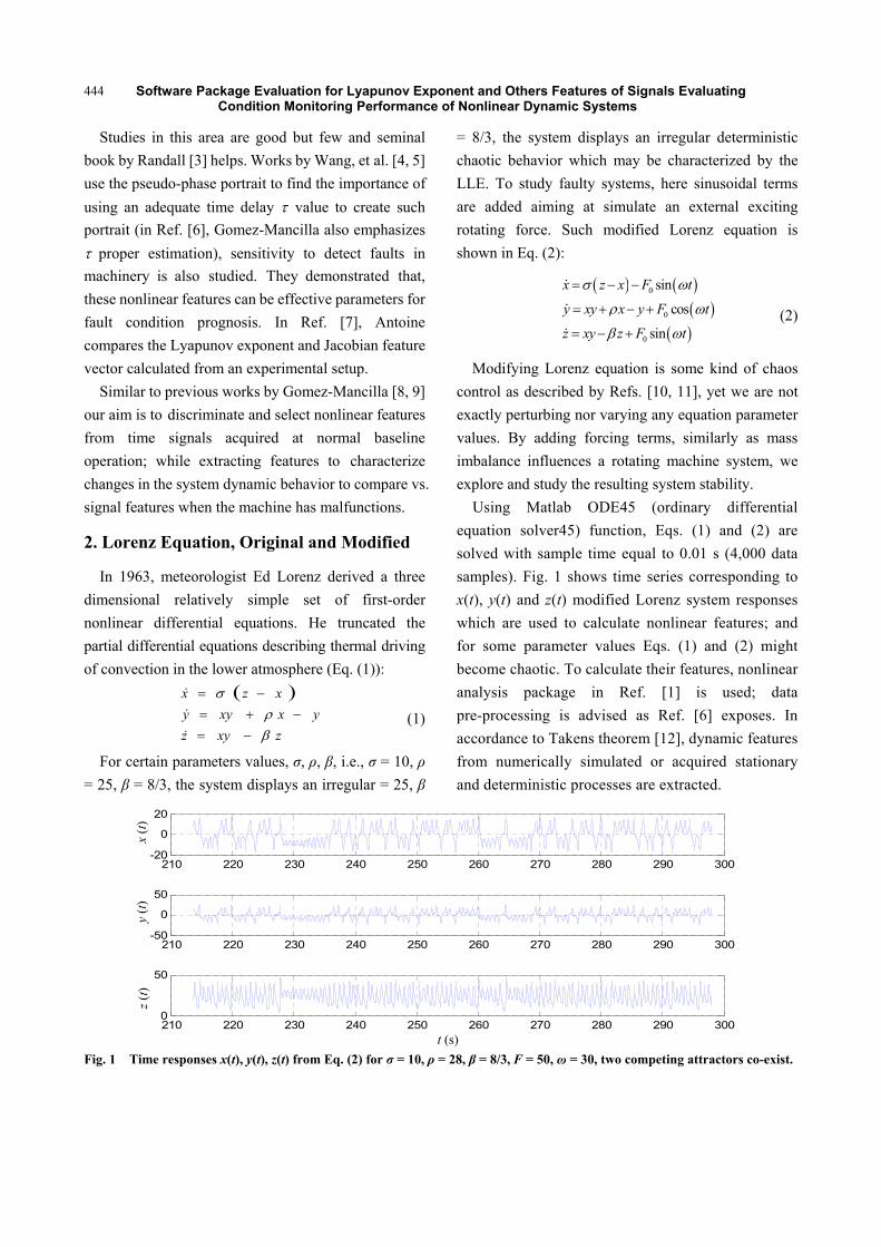
Using Matlab ODE45 (ordinary differential

equation solver45) function, Eqs. (1) and (2) are

solved with sample time equal to 0.01 s (4,000 data

samples). Fig. 1 shows time series corresponding to

x(t), y(t) and z(t) modified Lorenz system responses

which are used to calculate nonlinear features; and

for some parameter values Eqs. (1) and (2) might

become chaotic. To calculate their features, nonlinear

analysis package in Ref. [1] is used; data

pre-processing is advised as Ref. [6] exposes. In

accordance to Takens theorem [12], dynamic features

from numerically simulated or acquired stationary

and deterministic processes are extracted.

t (s)

Fig. 1 Time responses x(t), y(t), z(t) from Eq. (2) for σ = 10, ρ = 28, β = 8/3, F = 50, ω = 30, two competing attractors co-exist.

210 220 230 240 250 260 270 280 290 300-20

0

20

210 220 230 240 250 260 270 280 290 300-50

0

50

210 220 230 240 250 260 270 280 290 3000

50

x (t

) y

(t)

z (t

)


445

3. Nonlinear Time Series Analysis

Nowadays, condition monitoring by different signal

processing methods (frequency and time domain

analysis, wavelet, etc.), can be realized. Yet, potential

irregular nonlinear behavior arising from presence of

malfunctions in actual machines motivates the use of

powerful tools from nonlinear analysis. Following

steps aim at calculating the LLE [1]. First, obtain a

proper τ and embedding dimension m values by

mutual information [13] and false nearest neighbor

methods [14], respectively. Next, ensure input data

requirements are satisfied by testing if the system is

deterministic [15] and stationary [16]. Then, using a

single time series should verify if the reconstructed

phase or embedded space seems congruent. Finally,

using Wolf algorithm [17, 18], calculate the LLE and

determine if the system is chaotic, or not.

3.1 Embedded Space Reconstruction

The reconstruction generates information about the

unobserved (not measured) data, which allows

predicting the rest of the state variables. Mathematical

description is based on Takens’ theorem [12], where

using a single scalar time series x(t) can be enough to

reconstruct the state space. The previous since the

coordinates are related to each other through a time

delay (τ) [6, 13]. If τ is very small, then coordinates xt

and x(t + (m – 1)τ) are numerically so close to each other,

that can not be distinguished from each other. On the

contrary, if τ is too large, then xt and x(t + (m – 1)τ)

become independent of each other, in a statical sense.

Having properly determined τ, the information

obtained about other coordinates is large enough to

allow us to introduce values at times (t + τ, t + 2τ, …,

(t + (m – 1)τ) to substitute for the original coordinates.

An embedding space having same/similar features as

the original system, is therefore recreated (Eq. (3)).

2 1( ) , , , ...,t t t t mp t x x x x (3)

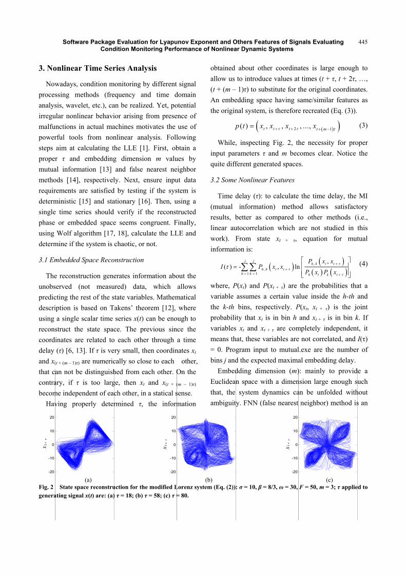
While, inspecting Fig. 2, the necessity for proper

input parameters τ and m becomes clear. Notice the

quite different generated spaces.

3.2 Some Nonlinear Features

Time delay (τ): to calculate the time delay, the MI

(mutual information) method allows satisfactory

results, better as compared to other methods (i.e.,

linear autocorrelation which are not studied in this

work). From state xt + τ, equation for mutual

information is:

,

,1 1

,( ) - , ln

j jh k t t

h k t th k h t k t

P x xI P x x

P x P x

(4)

where, P(xt) and P(xt + τ) are the probabilities that a

variable assumes a certain value inside the h-th and

the k-th bins, respectively. P(xt, xt + τ) is the joint

probability that xt is in bin h and xt + τ is in bin k. If

variables xt and xt + τ are completely independent, it

means that, these variables are not correlated, and I(τ)

= 0. Program input to mutual.exe are the number of

bins j and the expected maximal embedding delay.

Embedding dimension (m): mainly to provide a

Euclidean space with a dimension large enough such

that, the system dynamics can be unfolded without

ambiguity. FNN (false nearest neighbor) method is an

(a) (b) (c)

Fig. 2 State space reconstruction for the modified Lorenz system (Eq. (2)): σ = 10, β = 8/3, ω = 30, F = 50, m = 3; τ applied to generating signal x(t) are: (a) τ = 18; (b) τ = 58; (c) τ = 80.

-20

-10

0

10

20

-20

-10

0

10

20

X 1+

-20

-10

0

10

20

X 1+

x 1+τ

x 1+τ

x 1+τ


446

efficient algorithm that determines the minimum

embedding dimension (m), see for instance [14]. The

number of neighbors change along the signal path: 21

2

0

[ ]m

rD n kt n k t

k

r x x

(5)

Adding the proper time delay, transforms m to m + 1,

creating a new coordinate system, if the distances

change from one to another dimension, they are called

false neighbors. Previous method is implemented and

input to the fnn.exe code are τ, and the minimal and

maximal embedding dimension bound for which the

FNN is to be determined.

A deterministic system occurs when through a set of

ordinary differential equations, an initial state can

determine its future state. Uniqueness of solutions is

the property on which determinism test is built up.

Kaplan and Glass [15] proposed that determinism test

is required (where optimal k is equal to 1). The vector

field approximation for Vk in the k-th box of the phase

space is the average vector of all passes obtained

according to Eq. (6), Pk is the number of all passes

through the k-th box. The code determinims.exe

calculates a unique determinism parameter, inputs are

time delay and number of data points.

1

1 KP

K iiK

V eP

(6)

The code stationarity.exe indicates if the system

properties are kept constant during the data acquisition

process. Kantz and Schrieber [2] propose to compare

properties in one time series segment to another segment

acting as a data base, and call it cross-prediction error,

where, xt + Δt is the based value, x~t + Δt is the predicted

value and N is the number of trials made. Error should

be minimal for a stationary system since xt and a

neighbor pertain to the same data segment, this is

implemented into the stationarity.exe code.

2

1

1 N

t t t tk

x xN

(7)

3.3 LLE

Lyapunov exponents deserve a special place,

considering the divergence or convergence of nearby

orbits they determine the system dependence on its

initial conditions. An m dimensional system has m

possible Lyapunov exponents; existence of positive

LLE defines its unstable directions. The lyapmax.exe

code implements Wolf, et al. algorithm [17]; input

parameters are τ and m, then the LLE is calculated

from:

( )1log

( )

x t T

T x t

(8)

Applying Wolf theory, the implicit numeric LLE

calculation to each of the three (Eq. (2)) post-processed

response results are compared. Based on the system

Jacobian J, implicit numeric calculation estimates the

perturbation exponential growth δx:

d( )

d

xJ x x

t

(9)

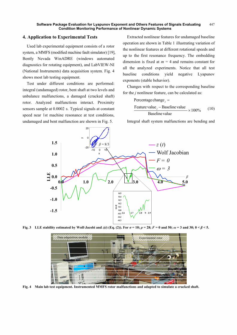
Fig. 3 shows how varying the “imbalance” and β

parameters induces significant changes in the system

stability, in β regions where the system is chaotic

unstable; for instance and specifically, F = 50 and ω =

3 r/s, are capable to control the system and turn it

stable. While, varying β parameter, instability and

stability are predicted by positive and negative LLE

values, respectively. Except for the purple line

analyzing z(t) response, all LLE values are calculated

by the Wolf-Jacobi algorithm numerically applied to

Eq. (2); recall that this implicit procedure [1, 17] does

not require individual analysis for each system signal

response. Using typical σ = 10, ρ = 28, range 0 < β < 5,

Fig. 3 considered three distinct cases:

(1) typical unperturbed Lorenz Eq. (1), red color

line;

(2) imbalance forced Lorenz Eq. (2), F = 50, ω = 30 r/s,

calculated both ways: by Wolf-Jacobi algorithm

shown by blue line, and also applying Perc package [1]

to z(t) shown by purple line;

(3) imbalance controlled Lorenz, Eq. (2), F = 50, ω

= 3 r/s, green color line. Notice three new system

stability β regions, including at the dreadful value β =

8/3 where a stable limit cycle orbit occurs.


447

4. Application to Experimental Tests

Used lab experimental equipment consists of a rotor

system, a MMFS (modified machine fault simulator) [19],

Bently Nevada WinADRE (windows automated

diagnostics for rotating equipment), and LabVIEW-NI

(National Instruments) data acquisition system. Fig. 4

shows most lab testing equipment.

Test under different conditions are performed:

integral (undamaged) rotor, bent shaft at two levels and

unbalance malfunctions, a damaged (cracked shaft)

rotor. Analyzed malfunctions interact. Proximity

sensors sample at 0.0002 s. Typical signals at constant

speed near 1st machine resonance at test conditions,

undamaged and bent malfunction are shown in Fig. 5.

Extracted nonlinear features for undamaged baseline

operation are shown in Table 1 illustrating variation of

the nonlinear features at different rotational speeds and

up to the first resonance frequency. The embedding

dimension is fixed at m = 4 and remains constant for

all the analyzed experiments. Notice that all test

baseline conditions yield negative Lyapunov

exponents (stable behavior).

Changes with respect to the corresponding baseline

for the j nonlinear feature, can be calculated as:

Percentagechange

Featurevalue Baselinevalue100%

Baselinevalue

j

j

(10)

Integral shaft system malfunctions are bending and

Fig. 3 LLE stability estimated by Wolf-Jacobi and z(t) (Eq. (2)). For σ = 10; ρ = 28; F = 0 and 50; ω = 3 and 30; 0 < β < 5.

Fig. 4 Main lab test equipment. Instrumented MMFS rotor malfunctions and adapted to simulate a cracked shaft.

-1.5

-1.0

-0.5

0.0

0.5

1.0

1.5

0.0 1.0 2.0 3.0 4.0 5.0LL

E

z(t)

Wolf-Jacobian

F=0

w=3

-0.3

-0.2

-0.1

0.0

0.1

0.2

0.3

0.4

0.5

2.6 2.7 2.8 2.9

LL

E

b

-10 0 10-20

0

20

x

y

=8/3 z(t)

Wolf Jacobian

F = 0

= 3

Data adquisition module Experimental rotor

z (t) β = 8/3

β


448

(a) (b)

Fig. 5 Filtered proximitor signals from an MMFS integral system rotating near first resonance (normalized frequency ω/ωn = 0.89): (a) baseline integral system; (b) system with a malfunction (level 1 bending).

Table 1 Extrated nonlinear features at baseline operation, different normalized rotation speeds /n.

/n 0.445 0.455 0.500 0.650 0.660 0.890 0.910 1.000

Time delay 32 31 30 32 31 29 31 29

Cross prediction error 0.0332 0.0365 0.0395 0.0321 0.0397 0.0412 0.0385 0.0370

Determinism 0.865 0.843 0.895 0.885 0.843 0.938 0.895 0.920

LLE -0.943 -0.958 -0.693 -0.780 -0.808 -0.595 -0.690 -0.490

unbalance. They are classified as: bending levels 1, 2

and 3, and only level 1 unbalance (unbalance mass

equal to 0.5 g). Two shafts damage are: crack depth

level 1 means 10% crack depth normalized by the

diameter; and crack depth level 2 is a 30% normalized

crack depth. Malfunction combinations are analyzed.

Increase in malfunction and damaged levels are

introduced into the MMFS test set up, signals are

acquired, filtered using nonlinearnoisereduction.exe

code and then numerically processed. Such

non-conventional filtering carefully treats the signals

as to not overly suppress nonlinear data which might

contain relevant malfunction information. The

de-noising procedure has a relevant positive effect on

the routines input parameters and strongly impacts all

the calculation results.

Nonlinear features performance: Five nonlinear

features trends and patterns are evaluated by a series of

lab test with known conditions. Table 2 shows

extracted features including LLE, τ, m, determinism

and cross-prediction error values compiled from Figs. 6a

and 6b plots, yielding adequate values close to zero,

0.010 and 0.020. Previous signal extracted values

insure fulfilment of the stationary requirement, which

also are Lyapunov stable (i.e., LLE negative). On the

other hand, although in Fig. 6c 2-D graph shows no

local error minimization along the 45 degree angular

orientation and a small average error of 0.040, it has a

high maximum error, 0.069. Moreover, positive LLE >

0, clearly indicates a chaotic unstable machine

behavior. Test signal for this cracked rotor case is

shown in Fig. 7, where chaos can not be perceived by

mere ball eye inspection. The other feature seemed less

sensitive to malfunctions: determinism does not have

sensitivity to detect malfunctions. While, different

kinds of errors directly evaluating the stationarity

dynamic characteristic might have certain small

diagnosing potential.

In Fig. 8, left-right sense along the horizontal axis

indicates a worsening of machine condition. In Fig. 8a,

both embedded dimension and determinism show low

sensibility to increasing worsening malfunction level,

with the exception for a highly damaged machine

which has stronger nonlinear dynamics and jumps

from m dimension 2 to 4. While in Fig. 8b, a

fluctuating yet slight increasing trend, can be perceived

in the time delay feature, while, the average

cross-predicted error values seem to fluctuate with no

1.5

1.0

0.5

0.0

‐0.5

‐1.0

‐1.50.0 0.5 1.0 1.5 2.0 2.5 3.0 3.5 4.0

x 10‐6

time (s)

Amplitude of vibration (m)

0.0 0.5 1.0 1.5 2.0 2.5 3.0 3.5 4.0Time (s)

Amplitude of vibration (m)

2.0

1.5

1.0

0.5

0.0

‐0.5

‐1.0

‐1.5

‐2.0

‐2.5

x 10‐6

Soft

clear trend.

damaged sys

the worse le

Fig. 6 Statio

Table 2 Non

Bend_1

Bend_2

Bend 2 + Unb

Crack_1

Crack_1 + Un

Crack_2

Fig. 7 Crack

i

tware PackagCon

Fig. 9 show

stem operatin

evel induced

onarity cross-p

nlinear feature

Time delay

35

31

b 48

31

nb 45

44

k level 2: (a) fi

ge Evaluationndition Monit

ws the LLE

ng at 6 malfu

d to the MMF

j (a)

predict error 2

es calculated fo

y Emb. dimm 2

2

2

2

2

4

(a)

ltered time ser

i

n for Lyapunotoring Perform

feature for

unction, inclu

FS (i.e., ben

-D plots obtain

or six different

mension Dete

0.99

0.99

0.99

1.00

0.99

0.98

ries; (b) zoome

ov Exponent mance of Non

r the

ding

ding

leve

incr

the

j (c)

ned from test:

t test rotor mal

erminism

97

99

99

00

99

84

ed view perform

i

and Others Fnlinear Dynam

el 3 and crack

rease of the L

machine wor

(a) bend_2; (b

lfunction sever

Error_min

0.013

0.010

0.015

0.013

0.004

0.012

med in previou

.0

Features of Simic Systems

k level 2). No

LLE feature,

rsening condi

j (b)

b) bend_2 plus

rity cases.

Error_avg

0.02

0.01

0.02

0.02

0.01

0.04

(b)

us time series.

ignals Evalua

otice a clear m

which is co

ition.

unbalance; (c)

Error_max

0.054

0.018

0.035

0.035

0.025

0.069

ating 449

monotonically

ngruent with

) crack_2.

LLE

-9.35

-7.06

0.61

8.98

3.02

3.15

.0

9

y

h


450

(a) (b)

Fig. 8 Left-right sense along horizontal axis indicates worsening machine malfunction severity level: (a) embedded dimension and determinism features; (b) embedded time delay τ and average cross-predicted error.

Fig. 9 The LLE feature shows a clear increasing trend, congruent with the machine malfunction severity level.

5. Conclusions

Increased availability of industrial equipment, safety and economic issues motivate research in maintenance programs based on monitored operating conditions. Machine behavior might turn nonlinear when operating with malfunctions. Typically linear excitation forcing terms are difficult to characterize, while nonlinear dynamics inducing large amplitude and/or chaotic behavior (i.e., certain deep breathing cracked shafts) are less difficult to identify. Five nonlinear features are extracted where the LLE displays higher sensitivity to machine malfunctions, since corresponding Lyapunov exponent feature tends to exhibit a decreasingly stability margin.

Moreover, to find potential reasons that would explain why most lab test signals obtained from malfunctioning equipment seemed dynamically sound, stability calculations extract nonlinear features from signals coming from actual machine test, and numerically, simulating an externally forced Lorenz system. Added forcing terms are similar to a rotating

mass imbalance influence. Next using Chaos Control similar concepts, i.e., vary the “mass imbalance” forcing parameters we aim to stabilize such modified Lorenz equation. Again both Wolf algorithms: Jacobian and that implemented by Perc M. are used.

Quite interestingly for certain values of the

imbalance excitation in Eq. (2), the system can be

stabilized, the previous even when paradigmatically

chaotic parameters for Lorenz system are used, see

Fig. 3. This quasi control approach is validated

studying signals obtained from previously mentioned

lab test (Fig. 9), where residual mass imbalance is

omnipresent in the test.

Finally, it is concluded that, analyzing and

comparing baseline vs. malfunction extracted

nonlinear features (acquired from equipment) can

increase the performance of machine condition

monitoring.

Acknowledgments

Authors acknowledge the CONACYT (National

Council for Science and Technology), IPN (National

Polytechnic Institute) and TecNM (National

Technologic of Mexico) for sabbatical year at Trieste

University, Italy for prof. Gomez and for scholarships

received.

References

[1] Perc, M. 2006. “Introducing Nonlinear Time Series Analysis in Undergraduate Courses.” Fizika A (Zagreb) 15 (2): 91-112.

Bend_1 Bend_2Bend+U

nbCrack_1

Crack_1+Unb

Crack_2

Dimension 2 2 2 2 2 4Determinism 0.997 0.999 0.999 1.000 0.999 0.984

0.975

0.980

0.985

0.990

0.995

1.000

1.005

0

0.5

1

1.5

2

2.5

3

3.5

4

4.5

Det

erm

inis

m

Dim

ensi

on

4.0

3.0

2.0

1.0

0.0 Bend_1

Bend_2

Bend+Unb

Crack_1

Crack_1+Unb

Crack_2

Time Delay 35 31 48 31 45 44Error_ave 0.02 0.01 0.02 0.02 0.01 0.04

0.00

0.05

0.10

0.15

0

10

20

30

40

50

60

Err

or_

ave

Tim

e D

ela

y

Time delay

Tim

e d

ela

y

Bend_1 Bend_2Bend+Unb

Crack_1

Crack_1+Unb

Crack_2

LLE -9.35 -7.06 0.61 8.98 3.02 3.15

-15

-10

-5

0

5

10

LL

E

Chaotic unstable

Lyapunov stable behaviour


451

[2] Kantz, H., and Schrieber, T. 2004. Nonlinear Time Series Analysis. Cambridge: Cambridge University Press.

[3] Randall, R. 2011. Vibration-Based Condition Monitoring. New Delhi: Wiley.

[4] Wang, B., and Lin, R. 2003. “The Application of Pseudo-phase Portrait in Machine Condition Monitoring.” Journal of Sound and Vibration 259 (1): 1-16.

[5] Wang, B., and Zhaohui, R. 2012. “Study on Fault Diagnosis of Rotating Machinery based on Lyapunov Dimension and Exponent Energy Spectrum.” Advanced Materials Research 591-593 (November): 2042-5.

[6] Gomez-Mancilla, J. C., Huesca-Lazcano, E., Palacios-Pineda, L., and M’Sirdi, N. 2015. “Signal Treatment Method to Properly Extract the Time Delay Feature to Characterize Nonlinear Systems.” MGEF (Mediterranean Green Energy Forum), Marrakech, Morocco.

[7] Antoine, C. 2011. “An Alternative to Lyapunov Exponent as Damage Sensitive Feature.” Smart Materials and Structures 20 (2): 025017.

[8] Gómez-Mancilla, J. C., Sinou, J. J., Nosov, V. R., Thouverez, F., and Zambrano, A. 2004. “The influence of Crack-Imbalance Orientation and Orbital Evolution for an Extended Cracked Jeffcott Rotor.” Comptes Rendus Mecanique 12 (332): 955-62.

[9] Machorro-Lopez, J. M., Adams, D. E., Gómez-Mancilla, J. C., and Gul, K. 2009. “Identification of Damaged Shafts Using Active-Sensing Simulation and Experimentation.” J. of Sound and Vibration 327 (3-5): 368-90.

[10] Heitor, F., Pereira-Pinto, I., and Ferreira, A. M. 2005. “State Space Reconstruction Using Extended State

Observers to Control Chaos in a Nonlinear Pendulum.” International Journal of Bifurcation and Chaos 15 (12): 4051-63.

[11] Eckehard, S., and Heinz, G. S. 2007. Handbook of Chaos Control. Weinheim: Wiley-VCH.

[12] Takens, F. 1981. “Detecting Strange Attractor in Turbulence.” In Lecture Notes in Mathematics, edited by Rand, D. A., and Young, L. S. Vol. 898. Berlin: Springer-Verlag, 366-81.

[13] Andrew, M. F., and Swinney, H. L. 1986. “Independent Coordinates for Strange Attractors from Mutual Information.” Physical Review 33 (2): 1134-40.

[14] Kennel, M. B., Brown, R., and Abarbanel, H. D. 1992. “Determining Embedding Dimension for Phase Space Reconstruction Using a Geometrical Construction.” Phys. Rev. A 45 (6): 3403-11.

[15] Kaplan, D. T., and Glass, L. 1992. “Direct Test for Deter-minism in a Time Series.” Phys. Rev. Lett. 68 (4): 427-30.

[16] Abarbanel, H. D. 1996. Analysis of Observed Chaotic Data. New York, NY: Springer-Verlag.

[17] Wolf, A., Swift, J. B., Swinney, H. L., and Vastano, J. A. 1985. “Determining Lyapunov Exponents from a Time Series.” Physica D 16 (3): 285-317.

[18] Shaw, R. 1981. Strange Attractors, Chaotic Behavior and Information Flow. Z. Naturforsch. A: CiteSeer.

[19] SpectraQuest, 2105. “MFS (Machinery Fault Simulator)”. SpectraQuest. Accessed December 12, 2014. http://spectraquest.com/products/simulators/machinery-fault-simulators.

Software Package Evaluation for Lyapunov Exponent …t), y(t) and z(t) modified Lorenz system...

Documents

Transcript of Software Package Evaluation for Lyapunov Exponent …t), y(t) and z(t) modified Lorenz system...