SoftwareforperformingfiniteelementanalysisThe purpose of these notes is to give an introduction to software available at RPI for performing finite element analyses. It is intended to give you a feel for the range of tools and point you to software that is available. Much of the information in this document is a function of time. The current version is addressing the state of the methods and software available in fall 2017. From a high level perspective the execution of a FE analysis is part of executing a simulation to evaluate one or more quantities of interest (QOIs) of a physical system for which the core mathematical model used is based on PDEs. Starting from that perspective the steps in performing the simulation using a FE method include:

1. Specifying the problem of interest – this should be done at the highest level possible. For problems we are considering this includes:

a. The domain of interest b. The physical attributes of loads, material properties, boundary conditions, initial

conditions. c. Indication of the QOI’s

2. Selecting the mathematical model(s) to represent the behavior – the PDE’s to be solved in our case. Step 1b must provide needed values for parameters that are part of the PDE.

3. Selecting the PDE discretization method – in our case FE methods. 4. Setting the mesh control information and generate and initial mesh and create analysis input

information. 5. Performing the finite element analysis 6. Evaluating the results with respect to mesh adequacy

a. If mesh not adequate, improve mesh and return to step 5 b. If mesh adequate, continue

7. Postprocessing the results to evaluate QOIs 8. Evaluating the modeling decisions

a. If models used not adequate, improve the models – if model is still PDEs return to step 3. b. If models adequate, continue

9. Preparing the final output information

ExecutionofSimulationWorkflowswithFEAnalysisThere are multiple modes taken in the execution of the simulation workflows that include finite element analysis analyses. The historic perspective for the execution of a FE analysis is to define all information directly in the form used in the input file the FE analysis code reads in for its execution. Tools were developed to ease the creation of these files, however, the means everything is defined in terms of a specific mesh making the execution of processes, such as adaptive analysis where the mesh changes, not only difficult, but also ambiguous. Although tools have advanced substantially, it is still common for tools to either allow, or even require, the specification of physical attribute information directly in terms of a given mesh. Reliable automation of simulation processes in which mesh discretization errors are adaptively addressed requires this information be defined in terms of a higher-level model representation. For example associating the physical attributes to entities in a CAD model for a fixed geometry simulation. There are higher-level models possible to deal with things like geometric shape/topology optimization and geometry evolution as part of the analysis (e.g., analyzing an additive manufacturing process).

SoftwareAvailableatRPIforSimulationswithFEAnalysisA number of tools needed to support finite element based simulations are available to RPI users. Many of these packages are available to the entire campus community while in other cases the software may only be available on specific systems or to specific research groups. The available software falls into one of two broad categories: open-source and closed source (typically commercial) software. In the majority of cases there is no issues in using an existing open source software package for academic use. However, it you are going to develop software building upon open

source software, you do need to check the form of open source license. Some licenses let you use and modify the software in any way you would like, while others require that all software that makes use of that software be made available as part the open source software. It is important to be aware of such license requirements since they can influence decisions you are able to make with software you develop. In the case of closed source commercial licenses must be obtained and there are typically restrictions on its use. In almost all cases it is limited to specific classes of academic only use. In some cases this can be limited to essentially classroom use while others also allow research use. In some cases the version that is available does not include all features, and/or limits the size of problem that can be addressed. To gain access to campus level software that you can download onto your own system go to the DOT CIO software install web page at http://dotcio.rpi.edu/services/software-labs A number of the software packages available to the RPI community are part of the PACE program. For more information on PACE see http://www.pace.rpi.edu/software.html In terms of running software on the RPI super computer and/or parallel clusters at the Center for Computational Innovations (http://cci.rpi.edu/), you can see the available software at https://secure.cci.rpi.edu/wiki/index.php/Software_overview To define a project and get a CCI account see https://secure.cci.rpi.edu/wiki/index.php/CCI_User_Wiki

GeometryGenerationSoftwareatRPIThere are multiple sources for the definition of the simulation domain. CAD models represent the most common domain definitions used in engineering processes. Other options for the definition of the domain include “mesh models” and “surface triangulations” where only a discretized version of the model is available, and “image data” in which basics information on material type at points of a regular grid is known. In the common case of the CAD model there is a topological model of the domain known in terms of material regions bounded by shells that are collections of faces that are bounded by one or more loops of edges that are bounded by vertices. The base topological entities of regions, faces, edges and vertices provide a convenient mechanism for the specification of the physical attributes since we are dealing with solving boundary value problems when solving PDE’s. It is also convenient to think of the mesh in terms of mesh regions, faces, edges and vertices, each of which can be associated with the geometric model entities. This supports the mapping of material properties, initial conditions and boundary conditions from the geometric model to any mesh used to represent the domain and supports proper mesh adaptation.

Solid modeling software that is available for use at RPI includes Siemens NX (formerly NX Unigraphics) and SolidWorks. See http://dotcio.rpi.edu/services/software-labs to download this software and its documentation. There is also tutorial information available as part of the basic engineering graphics and CAD course. Both of these solid modeling systems build upon the Parasolid Modeling Kernel which consists of a set of low level geometric model interrogation, creation, and modification functions. The Parasolid Modeling Kernel functions have been used by SCOREC researchers to develop specific

mesh region

mesh face

mesh edge

mesh vertex

region

region or face

region, face oredge

region, face,edge, or vertex

GEOMETRIC DOMAINENTITIES

MESHADJACENCIES

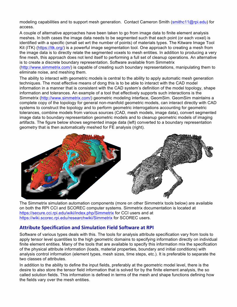
modeling capabilities and to support mesh generation. Contact Cameron Smith (smithc11@rpi.edu) for access. A couple of alternative approaches have been taken to go from image data to finite element analysis meshes. In both cases the image data needs to be segmented such that each point (or each voxel) is identified with a specific (small set wrt the number of points) of materials types. The Kitware Image Tool Kit (ITK) (https://itk.org/) is a powerful image segmentation tool. One approach to creating a mesh from the image data is to directly relate the segmented voxels to mesh entities. In addition to producing a very fine mesh, this approach does not lend itself to performing a full set of cleanup operations. An alternative is to create a discrete boundary representation. Software available from Simmetrix (http://www.simmetrix.com/) is capable of creating such boundary representations, manipulating them to eliminate noise, and meshing them. The ability to interact with geometric models is central to the ability to apply automatic mesh generation techniques. The most effective means of dong this is to be able to interact with the CAD model information in a manner that is consistent with the CAD system’s definition of the model topology, shape information and tolerances. An example of a tool that effectively supports such interactions is the Simmetrix (http://www.simmetrix.com/) geometric modeling interface, GeomSim. GeomSim maintains a complete copy of the topology for general non-manifold geometric models, can interact directly with CAD systems to construct the topology and to perform geometric interrogations accounting for geometric tolerances, combine models from various sources (CAD, mesh models, image data), convert segmented image data to boundary representation geometric models and to cleanup geometric models of imaging artifacts. The figure below shows segmented image data (left) converted to a boundary representation geometry that is then automatically meshed for FE analysis (right).

The Simmetrix simulation automation components (more on other Simmetrix tools below) are available on both the RPI CCI and SCOREC computer systems. Simmetrix documentation is located at https://secure.cci.rpi.edu/wiki/index.php/Simmetrix for CCI users and at https://wiki.scorec.rpi.edu/researchwiki/Simmetrix for SCOREC users.

AttributeSpecificationandSimulationFieldSoftwareatRPISoftware of various types deals with this. The tools for analysis attribute specification vary from tools to apply tensor level quantities to the high geometric domains to specifying information directly on individual finite element entities. Many of the tools that are available to specify this information mix the specification of the physical attribute information (loads, material properties, boundary and initial conditions) with analysis control information (element types, mesh sizes, time steps, etc.). It is preferable to separate the two classes of attributes. In addition to the ability to define the input fields, preferably at the geometric model level, there is the desire to also store the tensor field information that is solved for by the finite element analysis, the so called solution fields. This information is defined in terms of the mesh and shape functions defining how the fields vary over the mesh entities.

The figure below depicts the basics of applying attributes to a geometric domain while the figure on the right demonstrations the basics of a solution field.

The available tools for attribute specification and managing the solution fields range from geometry-based systems for applying tensor information to geometric model entities using either scripts or a graphical user interface, to tools that specify detailed pointwise information directly on the mesh. Many of the commercial finite element packages support the ability to specify the analysis attributes and store solution field data. Simmetrix has a graphical user interface for the specification of analysis attributes as well as a component (FieldSim) to manage the tensor fields associated with the geometric model and mesh. The pointer to Simmetrix software documentation is given at end of geometric modeling section. Note that the Simmetrix components can operate in parallel on distributed meshes. SCOREC also has a set of open source tools to manage meshes and fields associated with them. The core tool is PUMI/APF that supports the representation and manipulation of meshes and fields on distributed parallel computers. Pointers to information on PUMI/APF, as well as other SCOREC mesh based components can be found at https://www.scorec.rpi.edu/software.php.

MeshGenerationMany of the commercial analysis packages have mesh generation tools linked into the systems that can be exercised. In addition there are a number of both commercial and open source mesh generation tools that are available. In terms of campus usage for just doing finite element analysis, much of the mesh generation is done using tools that are part of a commercial finite element software system. It is now reasonably common that the mesh generation software can interact with geometry data from CAD systems. Although there have been substantial improvements in the ability to interact with such geometry, some mesh generation software more effectively interacts with CAD geometry than others. A number of the tools support the fully automatic generation of meshes from general geometries and provide various tools to specific information to control element sizes and gradations. The robust fully automated procedures are based on the use of simplex elements in at least major portions of the domain. One commercial mesh package available on campus is MSC Patran (http://www.pace.rpi.edu/software.html) Open source mesh generation tools include: • Triangle for 2D (https://www.cs.cmu.edu/~quake/triangle.html) • Gmsh for 3D (http://gmsh.info/) • CUBIT for hex meshing (https://cubit.sandia.gov/) • Netgen (https://sourceforge.net/projects/netgen-mesher/)

The Simmetrix mesh generation and mesh adaptation software, MeshSim and MeshSim Adapt, are heavily used in SCOREC in a large number of research projects. Like the other Simmetrix components,

they both can operate in parallel on distributed meshes. The pointer to Simmetrix software documentation is given at end of geometric modeling section. Some mesh generation examples:

The image cannot be displayed. Your computer may not have enough memory to open the image, or the image may have been corrupted. Restart your computer, and then open the file again. If the red x still appears, you may have to delete the image and then insert it again.

Figure 4: (left)Tetrahedral mesh of benchmark system containing 43 million elements and 7.8 mil-lion vertices. (right) Magnification of same mesh to show refinement near the interfaces withsolderballs. Approximately 40% of all mesh elements are within 1.5 radii of a solderball.

A mesh was generated for the benchmark configuration consisting of 43 million tetrahedralelements and 7.8 million vertices. This mesh is shown in Figure 4. The mesh for the benchmarkstructure, as well as those for other structural variations, are highly refined near the contact patcheson either side of the solder balls. In the benchmark mesh approximately 40% of all mesh elementsare located within 1.5 radii of the solderballs. The distribution of elements in and around a typicalcontact patch is shown on the right in Figure 4. It was found that with a thickness of 300 µm for theslabs representing the die and the chip carrier, the far side of each slab remained flat and variationsin stress across the back sides of the die and chip carrier, telegraphed through their thicknessesfrom the individual solder balls, were negligible.

We model the material properties of the die as that of pure silicon and those of the chip carrieras silica, as listed in Table 2. In each case, the die and carrier are regarded as being subject to J2plasticity but not to creep. The solder joints are modelled as being a Sn-Ag-Cu alloy with mostproperties taken from Ref. 15, and creep parameters taken from Ref. 16, as listed in Table 2.

2.3 Workflow

Our physical system is both geometrically complex and large compared to its smallest relevant ge-ometric feature and exhibits highly non-linear behavior over time. With such a large computationaltask, it is useful to employ large scale parallel computers for its solution. However, because wewish to simulate several geometric configurations of the already geometrically complex system,problem setup becomes a significant part of the total simulation effort. Our workflow for simulat-ing this system consists of generating the non-manifold geometric model, identifying parts of thegeometry that require highly refined meshing, constructing the mesh, partitioning the mesh into theappropriate number of parts for the parallel equations solver, applying the appropriate boundaryconditions within the solver, solving the mechanical equations, storing the solution, and analyzingthe results. Figure 5 shows how we implement this workflow.

To generate the geometric model, we use Siemens’ Parasolid modelling kernel [17] on a Linux-

7

Some adaptive mesh examples:

FiniteElementSoftwareatRPIThere are a number of software packages available at RPI that execute finite element, or finite volume, analyses. The list is known to be incomplete, thus do not be surprised to hear about other codes, particularly research ones associated with specific research groups. Most of the ones listed here are available to the RPI community or happen to be used regularly by multiple researchers in SCOREC. The available FE codes range in the types of physics they can model with codes for solid/structural mechanics, fluid mechanics, electromagnetics being most common. Some codes have been developed to be more general purpose and can deal with multiple classes of physics. Past the historic fact that many of the codes were originally targeted to a specific class of physical behavior, the “single physics” codes often contain a much richer set of capabilities to perform the engineering analyses related to that physical behavior. For example solid/structural mechanics codes not only have a broad range of appropriate material models, they have specific modeling capabilities such as beam, truss, plate and shell formulations as well as specialized modeling abilities such as fracture mechanics, etc. Similarly fluid flow codes will have specific fluid material models, turbulence models, specific boundary conditions, etc. The numerically intense part of these codes, the linear equation solvers, non-linear iteration procedures and time stepping procedures are also tailored to most effectively solve the large-scale non-linear ODE systems produced by those particular classes of problems. The codes that deal with multiple classes of physics usually have fairly standard models and solution procedures and require added care and, possibly development, for the engineering simulations of interest. The available codes also vary in terms license type and mode of use. The most fully featured codes tend to be commercial codes that have been under continuous development for years and are well supported. Commercial codes restricted to academic use that may be classroom and research, or class room only. Finite element codes available through the PACE project (see http://www.pace.rpi.edu/software.html include: • MSC NASTRAN is a solids/structural mechanics code that is well known for being able to address

structural dynamics problems. • Fluent is a finite volume based CFD code with lots of features.

• Altair HyperWorks a set of pre and postprocessing tools for setting-up finite element analyses. • See http://dotcio.rpi.edu/services/software-labs for the PACE software.

Other available commercial finite element codes are: • Abaqus (implicit) is a well known solid mechanics code that can effectively address nonlinear

behaviors. Useful information on using Abaqus is in a tutorial prepared by Prof. De http://www.ewp.rpi.edu/hartford/~ernesto/S2015/IFEM/Readings/AbaqusTutorial-De-RPI.pdf. There is both an educational version of Abaqus and a research version. The educational only supports very small problem sizes and can be downloaded from (http://dotcio.rpi.edu/services/software-labs) Because of the high cost of even research version of Abaqus there are only a limited number of licenses available. Thus there are times that all the licenses are checked out in which case additional users must wait.

• Altair AcuSolve is a powerful stabilized finite element based CFD code. It has excellent scalability for most classes of problems it addresses to a large number of cores. It is used in multiple SCOREC research projects. People with CCI accounts can find documentation on it at https://secure.cci.rpi.edu/wiki/index.php/AcuSolve. SCOREC user can find documentation at (https://wiki.scorec.rpi.edu/researchwiki/AcuSolve). Those that do not have a SCOREC account can contact Prof. Shephard – shephard@rpi.edu.

• ANSYS provides a number of packages that address for everything fluids, structures, electronics, multiphysics (http://www.ansys.com/). None of the ANSYS tools are currently available to RPI users, but we have been able to get licenses for specific use of specific packages in the past.

There are a number of open source codes used by various groups. Two that are supported commercially are: • FEniCS is a set of interoperable components that include a problem-solving environment, a form

compiler, a finite element tabulator, the just-in-time compiler, the code generation interface, the form language and a range of additional components. FEniCs is well suited for applications in which users wnat to implementation the weak form of a problem of interest. See https://fenicsproject.org for more information.

• Open Foam is primarily a CFD code that has been extended to support specific fluid flows involving chemical reactions and heat transfer plus specific coupled acoustics, solid mechanics and electromagnetics. See http://www.openfoam.com/.

SCOREC is involved in the development and/or extension of some open source codes: • PHASTA is an open source code CFD code which employs implicit stabilized finite element

technologies. It is developed jointly by RPI and UC Boulder. It has capabilities to handle incompressible and compressible flows, turbulent flows (with different levels of modeling ranging from RANS/URANS, DDES to LES), multiphase flows (with implicit and explicit tracking), complex geometry and adaptive meshing including boundary layer meshing, and massively parallel computation. PHASTA has been used in simulations approaching 100 billion elements using over 3 million MPI processes. PHASTA is heavily used in a number of research projects at RPI and other universities. SCOREC users see https://secure.cci.rpi.edu/wiki/index.php/PHASTA and https://github.com/SCOREC/phasta. For further information contact: Prof. Onkar Sahni <sahni@rpi.edu>.

• Albany is an implicit finite element from Sandia National Labs on is the Albany. Albany is part of the Trilinos https://trilinos.org/ object-oriented software framework making. Albany (see https://github.com/gahansen/Albany and https://github.com/gahansen/Albany/wiki) is implemented in C++ and requires a good understanding of modern C++ programming and meta-programming techniques to be able to effectively extend it. This makes Albany more flexible than a commercial finite element code (such as Abaqus or Altair) at the cost of a development overhead and a steep learning curve. An example of the adaptive capabilities SCORE has added to Albany can be seen in this ice-sheet example: https://github.com/gahansen/Albany/wiki/PAALS-Tutorial-2016 The premise of Albany is that a user should only need to implement the weak residual form of a finite element method, and the code should take care of assembling Jacobian matrices and residual

vectors 'behind the scenes'. This is done via a process called automatic differentiation. Additionally, Albany can perform sensitivity analyses using the same processes.

• MFEM is scalable C++ library for finite element methods (http://mfem.org/) from Lawrence Livermore National Laboratory. The goal of MFEM is to enable research and development of scalable finite element discretization and solver algorithms through general finite element abstractions, accurate and flexible visualization, and tight integration with the hypre library. Conceptually, MFEM can be viewed as a finite element toolbox that provides the building blocks for developing finite element algorithms. The SCOREC adaptive meshing procedures are being integrated into MFEM

ResultsPostprocessingThere are a number of postprocessing operations that are typically carried out ranging from simple examination of output vectors of nodal values to extensive uncertainty quantification operation using tools such as Dakota (https://dakota.sandia.gov/). One class of commonly applied postprocessing operations is the visualization of various solution fields. A number of commercial and open sources tools have been developed for the visualization of results. The most heavily applied tools are the VTK (serial) (http://www.vtk.org/) and ParaView (parallel) (http://www.paraview.org/) visualization tools from Kitware (http://www.kitware.com/). CCI users can find Paraview documentation at (https://secure.cci.rpi.edu/wiki/index.php/ParaView). Another heavily use package for parallel visualization is Visit https://wci.llnl.gov/simulation/computer-codes/visit/) from Lawrence Livermore National Laboratory. A few examples of types of visualization:

SomeCommentsontheExecutionofLargeScaleSimulationsHistorically all steps in a FE-based simulation workflow were executed in serial. This continues to be satisfactory for linear problem with up to 10,000 dof or so and for smaller time dependent and/or non-linear problems. Increasingly the level of computation needed to obtain acceptable accuracy for problems of interest requires much more computation that can only be effectively provided through the application of parallel computation. The current state of the art in industry is the application of some degree of parallel computation where up to 128 compute cores, or so, are applied in the execution of the FE analysis. All geometry and meshing steps are still executed in serial. Most postprocessing of the results is also done is serial or up to workstation level parallelism using tools like ParaView. Increasingly there is a push in research and, to some extend, industry to execute time-dependent, nonlinear analyses on meshes with billions of degrees of freedom. Such problems can only be run on large-scale parallel computers with 10’s of thousands, or more, of compute cores. Commercial CFD codes have been moving to large-scale parallel execution with many codes in the 10,000 core range and selected ones pushing 100,000 cores. The same is not true for commercial solid/structural codes that, for a number of reasons, are more difficult to scale. Their level of parallelism is much less than the fluids codes. On the research side the situation is different in that research codes are performing implicit solves on problems with 100 billion elements using more that 1 million processes and explicit codes have gone much larger. RPI’s Scientific Computation Research Center (SCOREC) (https://www.scorec.rpi.edu/) is one of the research groups pushing these limits. In addition RPI’s Center for Computational Innovations (CCI) (http://cci.rpi.edu/) houses one of the largest university based parallel super computers. Increasingly industry is looking at the potential of employing such large-scale simulations. For example simulations with well over 10 billion elements were part of the process that is leading Boeing to apply active flow control in next generation planes. When one pushes to the very large scale of problem, operations that were not a sizable portion of smaller scale parallel simulations become an issue. In particular it becomes necessary to perform all steps in the simulation workflow in parallel and the application of file I/O between component operations becomes a problem. Both Simmetrix and SCOREC have been developing the tools needed to be coupled with parallel finite element codes that allow all steps in an adaptive finite element simulation to be carried out in parallel using effective in-memory integration of the components. Simmetrix (http://www.simmetrix.com/) has tools to support parallel mesh generation, distributed mesh manipulation, distributed geometry and parallel mesh adaptation (contact Prof. Shephard shephard@rpi.edu for more information). SCOREC has developed open source tools for supporting distributed meshes, parallel mesh adaptation, dynamic load balancing (in conjunction with Sandia National Labs) and methods to support in-memory integration of simulation components. See https://www.scorec.rpi.edu/software.php for information on the software and https://www.scorec.rpi.edu/reports/ for papers on some of this work.