Software for Opto-Mechanical Modeling - Lambdares.com€¦ · · 2017-02-20Software for...

Software for Opto-Mechanical Modeling

Getting Started / Examples GuideRelease 7.4

Lambda Research Corporation25 Porter Road

Littleton, MA 01460

Tel.978-486-0766FAX978-486-0755

[email protected]@lambdares.com

mailto:[email protected]


COPYRIGHT AND TRADEMARK ACKNOWLEDGMENTS

COPYRIGHT

The TracePro software and manual are Copyright © 2014 by Lambda Research Corporation. Allrights reserved.

TRADEMARKS

TracePro and OSLO are registered trademarks of Lambda Research Corporation.

Pentium® is a registered trademark of Intel, Inc.

ACIS® is a registered trademark of Spatial Corporation.

Windows® XP, and Microsoft® are either registered trademarks or trademarks of MicrosoftCorporation in the United States and/or other countries.

ACCOS V™ is a trademark of Optikos Corporation.

Code V® is a registered trademark of Optical Research Associates, Inc.

ZEMAX® is a registered trademark of Focus Software, Inc. and Sigma™ is a trademark of FocusSoftware, Inc.

LIMITATIONS ON USE

The user of this Demo or Trial Version of TracePro is granted a license to use this product subjectto the following restrictions and limitations.

The user may not engage in, or permit third parties to engage in, any of the following:

• Providing use of the software in a computer service business or network

• Making alterations or excerpts of any kind in the software

• Attempting to disassemble, decompile, or reverse engineer the software in any way

• Attempting to defeat the software protection

TracePro Trial Version: Get Started / Examples Guide 2

TABLE OF CONTENTS

Introduction 4What is TracePro? 4What is the Restricted Demo Version? 4What Is the Trial Version? 4

System Requirements 4

Installing the TracePro Trial Version 6Running TracePro 6Running the TracePro Trial Version 7Get Started 7

Example Files 8

Stray Light in a Photolithography Lens 9Ray Tracing 10Flux Threshold 11

Metal Halide Lamp with Elliptical Reflector 13Defining Rays with Source Types 13

Integrating Sphere 17Importance Sampling 19

Creating Geometry 19

Luminaire 21

Eye Model 22

Importing Models 23

Gradient Index 24

Prisms 26

LCD Projector 27

Models 28

Sales & Technical Support Contacts 31


Introduction

What is TracePro?

TracePro is a comprehensive, versatile software tool for modeling the propagation of light inimaging and non-imaging opto-mechanical systems. Models are created by importing from a lensdesign program or a CAD program or by directly creating the solid geometry in TracePro. Sourcespropagate through the model with portions of the flux of each traced ray allocated for absorption,specular reflection and transmission, fluorescence and scattering. From the model, analyze:

• Light distributions in illumination and imaging systems

• Stray light, scattered light and aperture diffraction

• Throughput, loss, or system transmittance

• Flux or power absorbed by surfaces and bulk media

• Flux or power scattered by surfaces and bulk media

• Luminance and radiance maps

• Candela distributions

• Polarization effects

• Fluorescence effects

• Birefringence effects

TracePro has a simple, intuitive interface and short learning curve. It is compatible withcommercially available CAD programs such as SolidWorks®, AutoCAD®, Pro/E® and CATIA®. Itcan share solid modeling data with all other software based on ACIS, and exchange data withmost other CAD programs and analysis programs via IGES and STEP files. It can also import datafrom commercially available lens design programs including (OSLO, ACCOS V, Code V, Sigma,and ZEMAX). TracePro runs on Windows based PCs.

What Is the Restricted Demo Version?

The Restricted Demo Version of TracePro is a working copy of the software with certain keyfeatures disabled. Core functionality including geometry creation, ray tracing and analysis isenabled. Material and surface property data may be viewed but not edited. Example models areprovided that illustrate a sample of the addressable applications.

The Restricted Demo Version disables the following functionality:

• Saving models to disk

• Printing

• Applying optical properties to objects and surfaces

• Importing or exporting CAD files

• Macro processing

What is the Trial Version?

The Trial version is a temporary, 30-day license for you to try TracePro with all its functionality. Touse the trial version you must request a temporary license from Lambda Research.

System Requirements

TracePro requires a PC running Windows XP, Vista, 7 or 8. The amount of RAM available isimportant for TracePro performance. The amount of RAM needed depends on the specific


operating system and the complexity of the design you are simulating with TracePro. Therecommended configuration is Windows 7 x64 with 4GB or more of RAM. In general, the moreRAM the better. With more RAM you will be able to tackle larger problems with better performance.


Installing the TracePro Trial Version

You can download the Trial Version of TracePro from the Lambda Research web site. To install,simply run the installation program and follow the instructions.

To install TracePro from a CD, insert the CD into your drive and follow the installation instructions.

The installation program will create a TracePro74 folder on the Windows Start menu. A detaileddescription of all installation options is provided in the TracePro Installation Guide.

Running TracePro

FIRST TIME NOTE:

TracePro uses a database file, TRACEPRO.DB, to store all the properties that are used byTracePro. For example, the database contains material properties, surface properties, gradientindex properties, bulk scatter properties, and more. The first time you start TracePro, it will copythe TracePro.db file to your Windows Profile. In Windows XP, The TracePro.db file will be copied to

C:\Documents and Settings\username\Application Data\Lambda Research Corporation\TracePro,

and in Windows VISTA and Windows 7, it will be copied to

C:\Users\username\AppData\Roaming\Lambda Research Corporation\TracePro.

Next, TracePro will display the following dialog box offering to let you run TracePro indemonstration mode. Other options are available for licensed versions or more extensive Trialsand evaluations.

FIGURE 1 - TracePro License Information

Restricted Demo Mode

Single-computer License

Network License Data

Server host namefor Network

Licenses


Running the TracePro Trial Version

You will need a temporary license to run a TracePro Trial. The TracePro Trial is a full license of thesoftware, available for a limited time. Start TracePro and select Help|License in the License dialogbox, then select Single-computer license to access the temporary license provided to you byLambda Research.

Get Started

You can start by opening one of the prepared examples as described below. Many of the viewingfunctions (Zoom Window, Orbit View, Rotate View) are performed interactively using the mouse.For example, after opening any of the files, you can rotate the view using the Rotate View option.Press the Orbit Rotate View button on the toolbar (or select View|Rotate|Orbit from the menu),then move the mouse cursor inside the geometry window. Press and hold the mouse button down,move the mouse around, and watch the view change in real time as you move the mouse.

The Zoom Window command operates the same way as in a CAD program. Press the ZoomWindow button, press and hold the mouse button down at one corner of the region you would liketo zoom to, drag the mouse to the opposite corner of the region, and release the button. You canalso zoom in or out using the Zoom In and Zoom Out buttons.

TracePro features multiple views and multiple documents. Using the Window|New menu item (orthe New Window toolbar button), you can open as many views as you like of the current model.You can also have as many models open at one time as you wish, with as many views of each asyou wish as well. There are practical limits to this, of course, imposed by your computer’s memoryand screen area. You can choose from silhouette view (the default), rendered view, hidden line, orwireframe view using the View menu.

You can access context-sensitive help anytime by pressing F1 or by using the Help button on thetoolbar in TracePro.

Example Files

All example files are located on www.lambdares.com. To quickly access the Examples, startTracePro and select Help|TracePro Online, which will open your default web browser to theTechnical Support section of the web site. There you can log in, select TracePro and thenExamples, and finally, download any examples you would like to try.


Example - Stray Light in a Photolithography Lens

This model demonstrates a simple stray light analysis; analyzing ghost images in a refractive lenssystem. The model contains a multi-element lens system including lens barrels, retaining rings,and other mount design details. The lenses are made of Schott glasses. With the exception of thethird lens element that is uncoated, all lenses surfaces are modeled with anti-reflection coatingsand surface scattering. The non-optical surfaces are coated with diffuse black paint.

First download Lens_Demo.oml from the Lambda Research web site. (See “Example Files” onpage 7.) In TracePro, select File|Open and open the Lens_Demo.oml file. After the file is opened,you can display a side view of the lens will be displayed in the Model Window, as shown below, byselecting View|Silhouettes.

FIGURE 2 - Photolithography Lens Model

Now select View|Profiles|Iso 1 to see an isometric view of the lens system. You can also seea rendered view of the lens by selecting View|Render. Return to the y-z silhouette view by firstselecting View|Silhouettes, then selecting View|Profiles|YZ. Now we are ready to ray-tracethe model.

Select the Source of the System Tree on the left side of the Model Window. Click on the + next toGrid Source to expand the Frid Source tree, then double-click on Grid Source 1 (or single-click onit, then right-click and select Define|Grid Source) to open the Grid Source dialog box as shownbelow.


The settings specify a line of rays lying in the y-z (vertical) plane, and directed horizontally alongthe +z axis.

FIGURE 3 - Grid Source Dialog Box

Ray Tracing

Ray Tracing is the means by which TracePro simulates the distribution of flux throughout a model.How rays interact with the model is determined by the model itself (the geometry of created objectsand their applied properties), and how you control the rays being launched into the model. Thereare three basic methods of defining rays: Grid Sources, File Sources and Surface Sources.

The next step in this example is ray tracing. Select Raytrace|Trace Rays to start the ray-trace.

First, TracePro will perform an Audit of the model to ensure that all surface and material propertiesare in the database and to preprocess the geometry in the model for faster ray tracing. After theray-trace is finished, the rays will be displayed in the Model window as shown below.


FIGURE 4 - Ray Trace of Photolithography Lens Model

This ray-trace shows image-forming rays and some ghost rays caused by reflections from theuncoated element. The image-forming rays converge to a point at the image plane. The ghost raysare the ones reflected from lens element #3. They are terminated when their flux falls below theflux threshold, or go back out the front of the lens system.

Flux Threshold

The flux threshold is used to control the ray-trace. As rays are traced in the model, they are splitinto two or more components. For example, at the surfaces of lens element #3 in this model, theincident ray is split into two new rays, one transmitted and one reflected. The flux or power carriedby these split rays is proportional to the transmittance and reflectance of the surface. This splittingprocess occurs at each ray-surface intercept, with the flux of each ray segment decreasing at eachray-surface intercept. When the flux of the ray drops below the Flux Threshold, the ray isterminated. The flux threshold is controlled using the Raytrace|Raytrace Options dialog box.Select the Thresholds tab and change the Flux Threshold from 0.05 to 0.0002. Rerun the ray-trace. This will produce many more rays (and the ray-trace will take longer to finish). Some ghostrays will reach the image plane, causing stray light.

Imaging RaysGhost Rays


FIGURE 5 - Thresholds Tab in Raytrace Options Dialog Box

This example illustrates how TracePro can be used for stray light analysis. With its modeling ofscattering and its importance sampling feature, TracePro can predict stray light in telescopes andother optical systems that have high attenuation of stray light. By examining ray paths using theRay Sort feature, design alternatives to improve stray light performance are identified.


Example - Metal Halide Lamp with Elliptical Reflector

This example contains a simplified model of a metal halide lamp with an elliptical reflector,electrodes with a plasma arc and quartz enclosure, and an output plane. The arc is simulated as acylinder that radiates in a Lambertian pattern from its cylindrical surface.

First download EllipticalReflector.oml from the Lambda Research web site. (See “Example Files”on page 7.) Select File|Open and open the file. After the file is opened, a side view of the lens willbe displayed in the Model Window. Select View|Silhouettes to get the view shown below.

FIGURE 6 - Elliptical Reflector Model

On the left side of the Model Window is the System Tree. Items with a + in the System Tree can beexpanded by a single mouse click on the +. Once expanded, the + changes to a -. You cancollapse an expanded item by clicking on the -.

TracePro describes models as collections of Objects, each of which are bounded by one or moreSurfaces. For example, a sphere object has one bounding surface, and a cube object has sixbounding surfaces. Objects have Material Properties specified by name, like Glass or Aluminum,and Surfaces have Surface Properties, like Mirror, Lens, or Black Paint. Objects have mainbranches on the system tree, and surfaces have sub-branches.

Defining Rays with Source Types

Sources are defined as Grid, Surface and File. Grid Sources are defined as virtual windows to adistant source with rays emanating from the window. Surface Sources are applied as a property toan object’s surface. File Sources are comprised of external ray data read by TracePro during theray trace. Each of the source types can be defined from the Define menu or by Right-Clicking inthe Source Pane of the System tree.

The Source Pane in the System Tree is a central repository for all sources contained in the model.Each source is displayed as a node in a Source Tree. Expanding a node displays the varioussources of each type and further displays the relevant data for each source. Each source node ispreceded by a Green Check or Red X. Clicking on this flag will add or remove the source from thelist of sources to trace.


Any surface in a TracePro model can be made a source of light by making it a Surface Source.The cylindrical source in the eliprefl.oml example has a Surface Source property assigned to it.The total flux that will be emitted by the surface is 10 lumens and the emission will be simulatedusing 100,000 rays. The characteristics are shown above in the Model Pane of the System Treeand below in the Source Pane of the System Tree where a Green Check is set indicating it isenabled for raytracing.

FIGURE 7 - Source Pane in System Tree

The next step in this example is ray tracing. From the menu, select Raytrace|Trace Rays. Youcan also start the ray-trace by pressing the Trace rays button on the toolbar.

The progress of the ray-trace is displayed in the progress dialog and the ray-trace can beinterrupted at any time by pressing Cancel.

After the ray-trace is finished, rays will be displayed in the Model window as shown in the figurebelow. One focus of the ellipse is at the center of the cylindrical source, and the Front surface ofthe Observation Disk object is at the other focus. You can see the irradiance map for this surface,but first you must select it for viewing. To do this, expand the Observation Disk in the System Treeso that it looks like the figure below, and click on Front to select it.

Below is an Irradiance Map of the output. Select Analysis|Irradiance Maps (or press theIrradiance Maps button) to see this irradiance map.


FIGURE 8 - Ray Trace and Illuminance Map of Elliptical Reflector Model

You can also create a candela plot to see the angular distribution of light coming out of the lamp.Select Analysis|Candela Plots|Polar Iso-Candela to get the plot shown below. This is apolar plot of candela versus angle, and shows the intensity per unit solid angle, or lumens/steradian.

Select the Front Surfaceof the Observation Disk

Outline of SelectedSurface


FIGURE 9 - Polar Iso-Candela Plot of Elliptical Reflector

To create a candela plot, select Analysis|Candela Options to open the dialog box shown below.Set the Ray Selection to “Use incident rays from selected surface” and click Apply button.

FIGURE 10 - Candela Options Dialog

In the above Candela plot, if you move the mouse cursor over on the candela plot, the status bar atthe bottom of the TracePro window shows the angular coordinates and the candela value at thelocation of the mouse cursor. You can also display slices through this plot or a smaller squareregion within this polar plot.


Example - Integrating Sphere

This model simulates an integrating sphere to illustrate tracing of scattered rays and importancesampling. An integrating sphere is a hollow sphere with a highly reflecting, diffuse coating on theinside. Often an integrating sphere has an entrance port to let light in, and an exit port to let the(integrated) light escape. In this model, however, the sphere has only an exit port, and rays areemitted from a virtual source inside the sphere. This integrating sphere has a diffuse coating with99% reflectance on the inside.

First download IntegratingSphere.oml from the Lambda Research web site. (See “Example Files”on page 7.) Select File|Open and open the file.

FIGURE 11 - Integrating Sphere Model


This model has the flux threshold set to 5x10-5. This allows rays to scatter many times within thesphere before being terminated. To see how to set this threshold, select Raytrace|RaytraceOptions to open the dialog box shown below, and select the Thresholds tab.

FIGURE 12 - Raytrace Options Dialog box

Now open Source Pane in System Tree and notice that the number of rays for Grid Source 1 is setto one. Press the Trace rays button on the Analysis toolbar.

FIGURE 13 - Ray Trace of Integrating Sphere Model

The previous figure shows a close-up view of the integrating sphere output port for a singlestarting ray.


Select View|Zoom|Window (or press the Zoom Window button) then zoom in on the exit port at thebottom of the sphere to get the view shown on the previous page. Zooming to a window isdescribed in the “Get Started”.

As you can see, one starting ray produces many ray components as the ray scatters many timesinside the sphere. Each time a ray segment strikes the inside surface of the sphere, oneimportance sampling ray is directed toward the exit port of the sphere. This process of importancesampling greatly increases the sampling (i.e. number of ray components) at the exit port and thusimproves the efficiency of the ray-trace.

Importance Sampling

Importance sampling is a technique for improving the sampling in the Monte Carlo method. It isessential for studies like stray light analyses, wherein only a tiny fraction of the incident light

reaches the image surface. In a well-baffled telescope, 10-10, 10-15, or even less of the flux fromthe source may reach the image surface. In a “brute force” Monte Carlo raytrace in which rays findtheir way to the image surface by random scattering only (without importance sampling), anenormous number of rays must be traced to get only a few rays through the system. For example,

if 10-10 of the incident flux reaches the image surface, you must start 1010 rays to produce one rayat the image surface, on average.

In TracePro, importance sampling is a technique in which scattered rays are sent in specifieddirections in the optical system, such as toward the exit port of this integrating sphere. Theprobability of these rays reaching the exit port is thereby increased to one by this process, so theflux carried by them is reduced by the probability of them randomly reaching the exit surface. Thiscalculation is easily done by TracePro during the ray-trace and it assures that energy isconserved, i.e., that no “double dipping” takes place.

Creating Geometry

You can create the integrating sphere model geometry yourself, although the Trial Version doesnot allow you to apply the surface properties needed to do the ray-trace shown above. To createthe hollow sphere needed for the integrating sphere, you define two concentric solid spheres andsubtract the smaller one from the larger to create a spherical shell. To accomplish this, do thefollowing steps:

1. Select File|New or press the New button to open a new model window.

2. Select Insert|Primitive Solid and select the Sphere tab.

3. Enter 50 for the Radius and press the Insert button. A sphere will be drawn in the window.

4. Change the Radius to 51 and press the Insert button. A second sphere will be drawn.

5. Select Edit|Select|Object (or press the Select Object button on the toolbar) to enableObject Selection. Click on the Outer Sphere and, press and hold down the Ctrl key, then clickon the Inner Sphere. Zooming in on the edge of the spheres makes it easier to pick the rightone. You can also select items from the System Tree.

6. Select Edit|Boolean|Subtract (or press the Subtract button on the toolbar). Once youcomplete this, the inner sphere has been subtracted from the outer sphere to produce aspherical shell. (If you make a mistake, press the Undo button and try again.)

7. Select the Cylinder/Cone tab on the Insert|Primitive Solids dialog box to prepare tomake a cylinder. The cylinder will be used to make a hole in the bottom of the spherical shell.

8. For the cylinder set the Base Major R = 2, Top Length = 20, .

9. Set the Base Position Y = -49, Base Rotation X = 90, and press the Insert button. A cylinderwill be drawn at the bottom of the spherical shell. If you had previously zoomed in assuggested in 5. above, do Zoom All to see the cylinder.


10. Select the spherical shell and then the cylinder as shown in step 5. SelectEdit|Boolean|Subtract (or press the Subtract button on the toolbar). You have used thecylinder as a drill bit to drill a hole in the shell.

11. In the Cylinder/Cone tab of the Insert|Primitive Solids dialog box, set the cylinder TopLength = 1, and Base Major R to 2.5. Set the Base Position Y = -51 and the Base Rotation X= 90. Press the Insert button.

The geometry you have created in these 11 steps is identical to the integrating sphere model.


Example - Luminaire

This model simulates a fluorescent light fixture with louvers. The lamp is represented as a surfacesource and the typical output is these applications is a Polar Candela distribution.

First download Luminaire_Louver.oml from the Lambda Research web site. (See “Example Files”on page 7.) Select File|Open and open the file. The model will appear as shown below.

FIGURE 14 - Luminaire with Louvers Model

From the menu select Raytrace|Trace Rays. You can also start the ray-trace by clicking theTrace rays button on the toolbar. This model is set to trace 10,000 rays. Once the raytrace iscomplete select Analysis|Candela Plots|Polar Candela Distribution to get the plot shownbelow.

FIGURE 15 - Polar Candela Distribution Plot


Example - Eye Model

This model simulates light entering the eye. TracePro uses property information to describe howlight interacts with surfaces and objects (or volumes). The model with traced rays is shown below,along with a TracePro Flux Report.

First download EyeModel_CGBF.oml and EyeModel_CGBF_Properties.txt from the LambdaResearch web site. (See “Example Files” on page 7.) Select File|Open and open the file, thenselect Tools|Database|Import (or press F11 on your keyboard) and open theEyeModel_CGBF_Properties.txt file to import the properties needed for this model. Open theSource Pane in the System Tree and notice that Grid Source 1 is green checked for inclusion inthe ray trace. Press the Trace rays button on the toolbar to trace the currently defined grid. Themodel with rays is shown below.

FIGURE 16 - Eye Model

A Flux Report provides a table of flux distributions throughout the mode. Each surface and objectis shown with the number of incident rays, incident and absorbed flux, and other data. The report isshown below. The Flux Report is displayed using the Reports|Flux menu.

FIGURE 17 - Flux Report Table


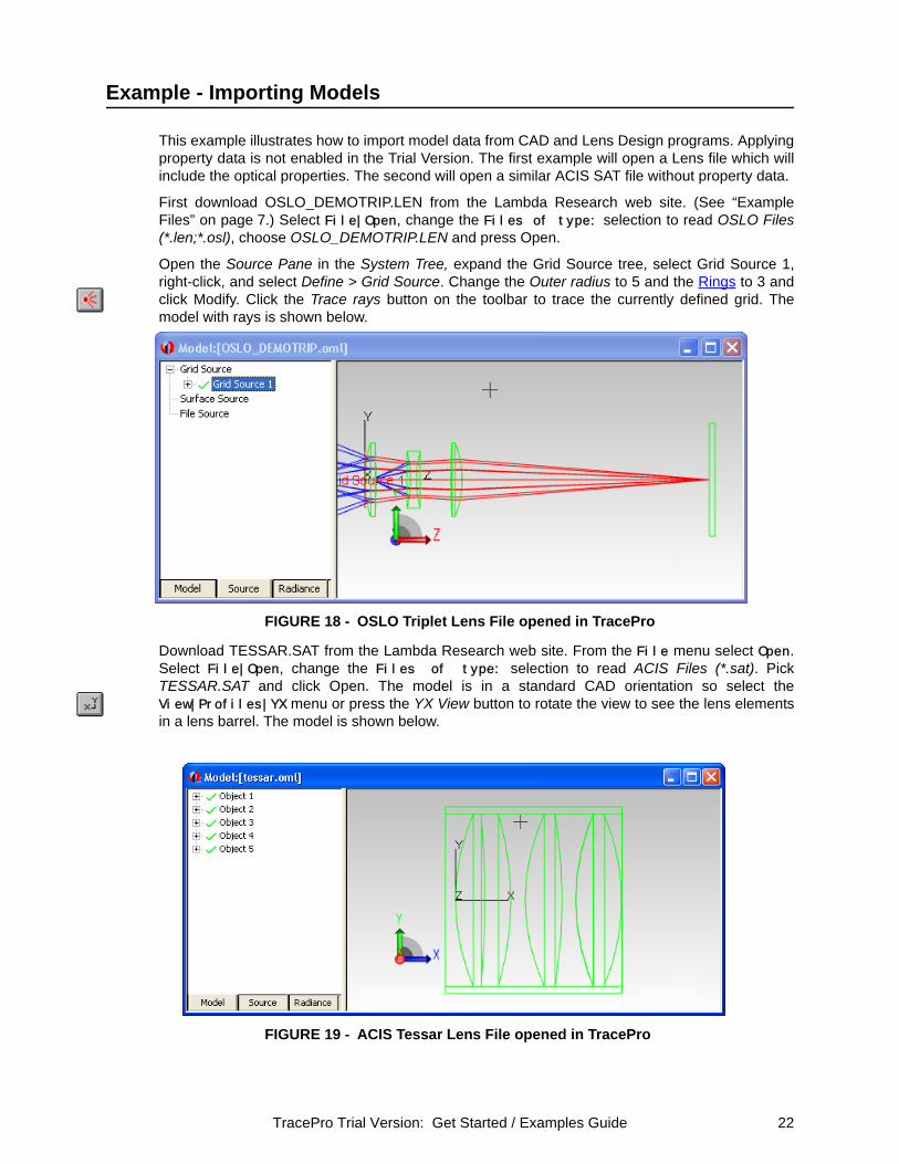
Example - Importing Models

This example illustrates how to import model data from CAD and Lens Design programs. Applyingproperty data is not enabled in the Trial Version. The first example will open a Lens file which willinclude the optical properties. The second will open a similar ACIS SAT file without property data.

First download OSLO_DEMOTRIP.LEN from the Lambda Research web site. (See “ExampleFiles” on page 7.) Select File|Open, change the Files of type: selection to read OSLO Files(*.len;*.osl), choose OSLO_DEMOTRIP.LEN and press Open.

Open the Source Pane in the System Tree, expand the Grid Source tree, select Grid Source 1,right-click, and select Define > Grid Source. Change the Outer radius to 5 and the Rings to 3 andclick Modify. Click the Trace rays button on the toolbar to trace the currently defined grid. Themodel with rays is shown below.

FIGURE 18 - OSLO Triplet Lens File opened in TracePro

Download TESSAR.SAT from the Lambda Research web site. From the File menu select Open.Select File|Open, change the Files of type: selection to read ACIS Files (*.sat). PickTESSAR.SAT and click Open. The model is in a standard CAD orientation so select theView|Profiles|YX menu or press the YX View button to rotate the view to see the lens elementsin a lens barrel. The model is shown below.

FIGURE 19 - ACIS Tessar Lens File opened in TracePro


Example - Gradient Index

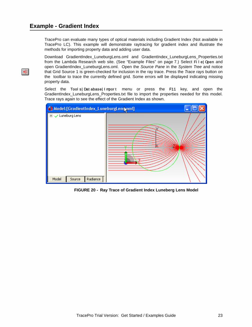
TracePro can evaluate many types of optical materials including Gradient Index (Not available inTracePro LC). This example will demonstrate raytracing for gradient index and illustrate themethods for importing property data and adding user data.

Download GradientIndex_LuneburgLens.oml and GradientIndex_LuneburgLens_Properties.txtfrom the Lambda Research web site. (See “Example Files” on page 7.) Select File|Open andopen GradientIndex_LuneburgLens.oml. Open the Source Pane in the System Tree and noticethat Grid Source 1 is green-checked for inclusion in the ray trace. Press the Trace rays button onthe toolbar to trace the currently defined grid. Some errors will be displayed indicating missingproperty data.

Select the Tools|Database|Import menu or press the F11 key, and open theGradientIndex_LuneburgLens_Properties.txt file to import the properties needed for this model.Trace rays again to see the effect of the Gradient Index as shown.

FIGURE 20 - Ray Trace of Gradient Index Luneberg Lens Model


Next, you can modify the property by opening the Gradient Index editor using the Define|EditProperty Data|Gradient Index Properties menu, select Luneburg Lens from the drop downlist, and press Edit|Unlock Property.

FIGURE 21 - Grin Property Editor Dialog

Change the nr1 coefficient to 2. Select File|Save to update the database and trace a GridRaytrace as above. TracePro automatically updates the model to use the new data. The updatedraytrace is shown below. Notice the shift in the focal point.

FIGURE 22 - Updated Ray Trace of Gradient Index Luneberg Lens Model

Change the value of nr1 from 1 to 2Lock/Unlock Icon


Example - Prisms

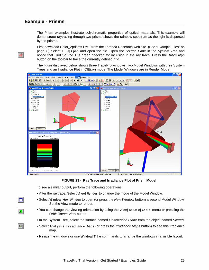
The Prism examples illustrate polychromatic properties of optical materials. This example willdemonstrate raytracing through two prisms shows the rainbow spectrum as the light is dispersedby the prisms.

First download Color_2prisms.OML from the Lambda Research web site. (See “Example Files” onpage 7.) Select File|Open and open the file. Open the Source Pane in the System Tree andnotice that Grid Source 1 is green checked for inclusion in the ray trace. Press the Trace raysbutton on the toolbar to trace the currently defined grid.

The figure displayed below shows three TracePro windows, two Model Windows with their SystemTrees and an Irradiance Plot in CIE(xy) mode. The Model Windows are in Render Mode.

FIGURE 23 - Ray Trace and Irradiance Plot of Prism Model

To see a similar output, perform the following operations:

• After the raytrace, Select View|Render to change the mode of the Model Window.

• Select Window|New Window to open (or press the New WIndow button) a second Model Window.Set the View mode to render.

• You can change the viewing orientation by using the View|Rotate|Orbit menu or pressing theOrbit Rotate View button.

• In the System Tree, select the surface named Observation Plane from the object named Screen.

• Select Analysis|Irradiance Maps (or press the Irradiance Maps button) to see this irradiancemap.

• Resize the windows or use Window|Tile commands to arrange the windows in a visible layout.


Example - LCD Projector

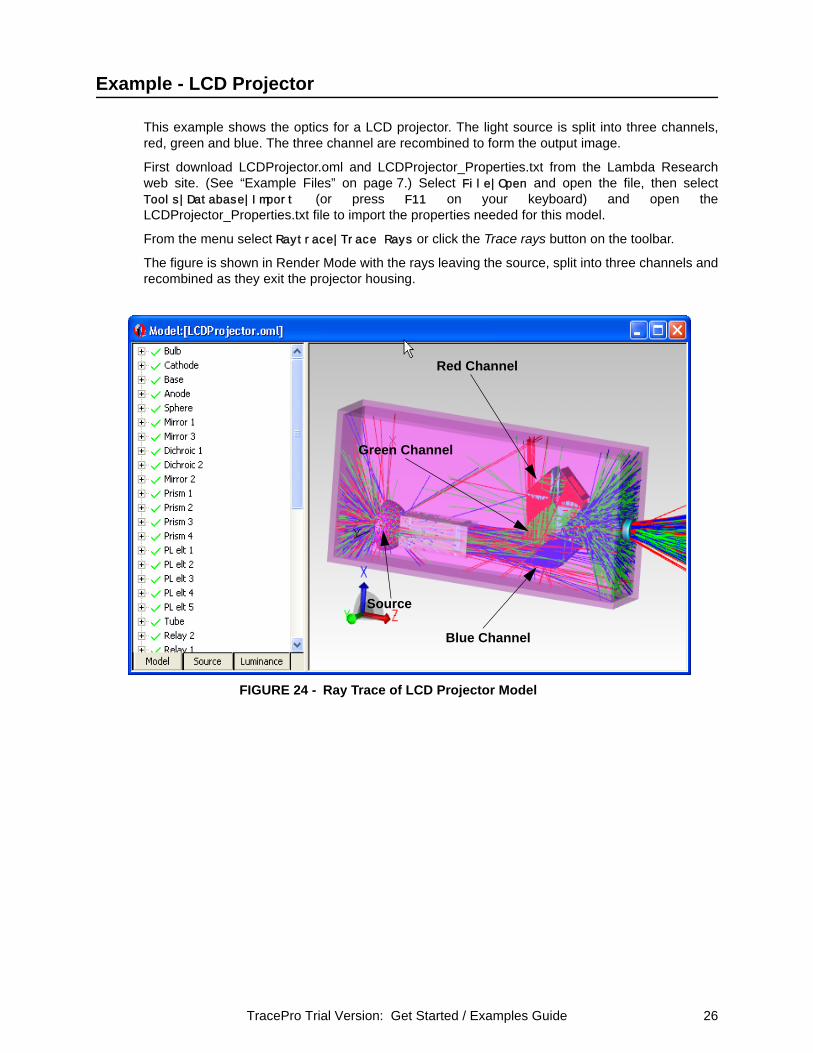
This example shows the optics for a LCD projector. The light source is split into three channels,red, green and blue. The three channel are recombined to form the output image.

First download LCDProjector.oml and LCDProjector_Properties.txt from the Lambda Researchweb site. (See “Example Files” on page 7.) Select File|Open and open the file, then selectTools|Database|Import (or press F11 on your keyboard) and open theLCDProjector_Properties.txt file to import the properties needed for this model.

From the menu select Raytrace|Trace Rays or click the Trace rays button on the toolbar.

The figure is shown in Render Mode with the rays leaving the source, split into three channels andrecombined as they exit the projector housing.

FIGURE 24 - Ray Trace of LCD Projector Model

Red Channel

Green Channel

Source

Blue Channel


Models

The TracePro Examples page in the Technical Support section of the Lambda Research web sitecontains model and property files. Follow the procedure described in the Examples Chapter toopen the *.oml model file and load the *.txt property data (if any) using the F11 key.


Sales and Technical Support Contacts

[email protected] [email protected]

You can find a current list of our representatives world-wide at our web site, www.lambdares.com


http://www.lambdares.com



Software for Opto-Mechanical Modeling - Lambdares.com€¦ · · 2017-02-20Software for...

Documents

Transcript of Software for Opto-Mechanical Modeling - Lambdares.com€¦ · · 2017-02-20Software for...