Software Architecture Considerations for Facilitating

Electric Power System Planning

Incorporating a Variety of Design Categories

Jeremy Woyak

Thesis submitted to the Faculty of the

Virginia Polytechnic Institute and State University

in partial fulfillment of the requirements for the degree of

Masters of Science in Electrical Engineering

Robert P. Broadwater (Co-Chair),

Binoy Ravindran (Co-Chair),

Virgilio Centeno

March 1, 2012

Blacksburg, Virginia

Keywords: Electric Power System Planning Software

Software Architecture Considerations for Facilitating

Electric Power System Planning

Incorporating a Variety of Design Categories

Jeremy Woyak

Abstract

This work investigates some of the features of existing software applications for electric

power system planning as well as some of the limitations that keep these applications

from being more frequently used in distribution planning. This work presents a software

framework that could facilitate much greater use of a wide variety of planning

applications.

An integrated system model (ISM) provides a centralized approach to storing data for

access by other planning applications. Additionally, an integrated performance simulator

(IPS) facilitates comparing the design projects generated by those various planning

applications across many criteria under various load growth scenarios. Furthermore, the

IPS can automatically run any number of validation routines on a given design or set of

designs, alerting the planning engineer of additional, unanticipated planning needs.

This paper provides three case studies which demonstrate the kinds of detailed evaluation

and visualization of trade-offs that an IPS could facilitate. The case studies further

highlight the greater levels of detail that may be utilized by the ISM and IPS in analyzing

any set of modular designs and load growth scenarios.

iii

Acknowledgments

I would like to thank Dr. Robert Broadwater for his support and assistance in this and all of my

work at Electrical Distribution Design, as well as for granting me the opportunity to come to

Virginia Tech and to work under his guidance and direction. His vision for power system

planning software is inspiring.

I would like to thank Electrical Distribution Design for providing software and models for me to

develop and evaluate the ideas expressed in this paper as well as for providing me with exciting

and challenging work to motivate this research. I am very appreciative of my co-workers

bringing me up to speed very quickly as I began to work at EDD.

In addition, I would like to thank the planning engineers at Detroit Edison and Electrical

Distribution Design for the insight they have provided in the limitations of existing power system

planning software as well as the kinds of features that they wish to see developed.

I would also like to express my gratitude to Dr. Ravindran and Dr. Centeno for serving on my

advisory committee and taking some of their valuable time to listen to my defense and consider

this work.

To my family and church family I would like to express my appreciation for their love,

encouragement, support, and prayers for me in this and all of my work.

Above all, I acknowledge and exult in the grace of my Lord and Savior, my God, whose name is

Father Son and Holy Spirit, for giving me every ability and opportunity that enabled me to

complete this work, for being more patient with me than I could ever know, for encouraging and

sustaining me in my efforts in this and all of the good works which He has prepared for me to do,

and for the many other ways in which He has shown me His grace which would require many

more pages than this paper to enumerate completely even in summary form.

iv

Table of Contents 1. Background ................................................................................................................................. 1

1.1 Technical Requirements........................................................................................................ 1

1.2 Load Growth ......................................................................................................................... 3

1.3 Planning Scenarios ................................................................................................................ 3

2. Current Planning Software .......................................................................................................... 4

2.1 The Role of Software in the Distribution Planning Process ................................................. 5

2.2 Power System Planning Models ........................................................................................... 6

2.2.1 Load Forecasting Models ............................................................................................... 6

2.2.2 Performance Simulation Models.................................................................................... 8

2.3 Decision Support Software ................................................................................................. 10

2.3.1 Searching the Solution Space....................................................................................... 11

2.3.2 Evaluating Alternatives ................................................................................................ 12

2.4 Past Success with Optimization .......................................................................................... 14

3. Proposed Planning Software ..................................................................................................... 15

3.1 Integrated System Model and Integrated Performance Simulator Overview ..................... 17

3.1.1 Integrated System Model ............................................................................................. 17

3.1.2 Independent Optimization Algorithms ........................................................................ 18

3.1.3 Integrated Performance Evaluator ............................................................................... 18

3.2 Modular Load Growth Scenarios and Modular Design Projects ........................................ 19

3.3 Automatic Design Validation ............................................................................................. 20

3.4 Intuitive Visualization of Multiple, Multi-dimensional Criteria......................................... 21

3.5 Open Architecture for Performance Simulators ................................................................. 22

3.6 Case Studies ........................................................................................................................ 23

3.6.1 Case Study 1: Phase Balancing to Resolve Overloads and Reduce Losses ................. 25

3.6.2 Case Study 2: Resolving Low Voltages....................................................................... 30

3.6.3 Case Study 3: Resolving Overloads ............................................................................. 42

3.6.4 Case Study Conclusions ............................................................................................... 49

4. Conclusions, Contributions, and Future Work ......................................................................... 50

4.1 Conclusions and Contributions ........................................................................................... 50

4.2 Future Work ........................................................................................................................ 51

v

5. References ................................................................................................................................. 53

List of Tables Table 1. Planning Process Steps and Software ............................................................................... 5

Table 2. Computer vs. Human Expertise ...................................................................................... 16

Table 3. Summary of First 2 Phase Balancing Moves .................................................................. 26

Table 4. Effects of Third Phase Move Options on Substation Exit Cable Currents ..................... 28

Table 5. Comparison of Loss Reductions for Each Third Phase Move Option ............................ 28

Table 6. Lowest Voltages On Feeder for Third Phase Move Options .......................................... 29

Table 7. Effects of Capacitor at Industrial Load on Minimum Feeder Voltages .......................... 32

Table 8. Loss Reduction from First Capacitor Addition............................................................... 32

Table 9. Comparison of Alternative Capacitor Placement Options .............................................. 36

Table 10. Capacitor Placement Comparison under Multiple Pricing Scenarios ........................... 40

Table 11. Load Growth Scenario 1 ............................................................................................... 43

Table 12. Load Growth Scenario 2 ............................................................................................... 46

List of Figures

Figure 1. Abstract Representation of a Model ................................................................................ 6

Figure 2. "S" Curves Depicting Load Growth Rates for Different Sized Areas ............................. 7

Figure 3. Sample Hourly Loss Curve and Price Data for One Day .............................................. 10

Figure 4. Sample Pareto-Optimal Set ........................................................................................... 14

Figure 5. Relationships between ISM and IPS and Independent Planning Applications ............. 17

Figure 6. Combinations of Modular Load Growth Scenarios and Alternative Designs ............... 20

Figure 7. Integration of Modular Load Scenarios and Modular Designs with ISM and IPS ....... 20

Figure 8. Dependencies Between Individual Planning Applications, the IPS, and the ISM ........ 23

Figure 9. Feeder Used in Case Studies ......................................................................................... 25

Figure 10. Multi-Dimensional Voltage Profile for Third Phase Move Options ........................... 30

Figure 11. Load Reach Plot to Customer Five Miles from Substation ......................................... 31

Figure 12. Voltage Profile Before and After Adding Capacitor at Industrial Load Center .......... 32

Figure 13. Load Reach After Adding Capacitor at Industrial Load Center .................................. 33

Figure 14. Load Reach Plot after Additional Capacitors .............................................................. 41

Figure 15. Loading Analysis for New Step Transformer under Load Growth Scenario 2 ........... 44

Figure 16. Number of BES Units Needed under Load Growth Scenario 1 .................................. 45

Figure 17. Voltage Comparison for Overload Solutions under Load Growth Scenario 1 ............ 45

Figure 18. Loading Analysis for New Step Transformer under Load Growth Scenario 2 ........... 47

Figure 19. Number of BES Units Needed under Load Growth Scenario 2 .................................. 48

Figure 20. Voltage Comparison for Overload Solutions under Load Growth Scenario 2 ............ 48

1

1. Background Modern electric power systems efficiently carry enormous amounts of energy extraordinary

distances with exceptionally high reliability. To do this efficiently, power systems transform

voltages several times, reaching extremely high voltages at the transmission level, yet

consistently delivering that power to millions of customers with relatively small variations from

an expected service-level voltage. The design and construction of such a vast, complex, reliable,

and efficient system is an engineering marvel.

The International Energy Agency reports that, in the United States alone, the electricity produced

each year is on the order of thousands of terawatt-hours [1]. Such an amount of energy is so far

outside normal human experience that very few Americans would be any more or less impressed

if that figure increased or decreased by a factor of one hundred. Equally amazing is the fact that,

in spite of the dangerously high voltages used, most users expect such great reliability of service

that loss of power for a mere one-tenth of one percent of the year (more than eight hours) would

flood the utility and regulatory agency with phone calls. Customers expect that their electric

service will be not only extremely reliable but also very inexpensive. Willis succinctly states

that, for many consumers, “electric energy…is cheap enough to waste” [2].

Customers enjoy not only a low electrical energy cost but also a stable electrical energy cost. In

spite of the fact that electric loads are changing every year, most customers neither see their

reliability degrade nor their costs increase. Though this last fact sounds considerably less

impressive than the aforementioned facts, it is a witness of not only excellent engineering, but

also shrewd economic planning.

If the planning engineer simply had to design a reliable, low-cost system for delivering a fixed

amount of load to certain customers, that alone would be an impressive task. The planning

engineer’s task, however, is not so simple. The system must not only serve current and known

near-term load increases; it must also have the capacity to serve additional load growth that

cannot be predicted with great certainty. The utility cannot afford to rebuild the system each time

the load increases. Nor can the utility afford to overbuild the system today for every possible

load increase for the next decade. An economic balance must be found between underbuilding

and overbuilding for future load growth.

1.1 Technical Requirements In addition to keeping costs low, the planning engineer is responsible for maintaining the

following criteria. Note that these requirements show the customer’s perspective, and different

customers will place different values on quality and reliability.

1. Every customer must have access to electrical power.

2

2. The electrical power delivered must meet certain criteria regarding quality (criteria

including frequency, voltage magnitude, rate of change of voltage, and harmonic

distortion).

3. The electrical power must meet certain reliability criteria at a system level (both the

frequency and duration of outages must meet certain criteria).

4. The design must be at or near minimum long-term cost.

The first requirement implies that a minimum amount of equipment must have been purchased,

delivered to the site, constructed/installed, and energized before the customer expects to begin

using the power. In order to meet all of these requirements, many additional engineering

constraints must be met. For example, good reliability depends on equipment being loaded

within thermal limits and being protected from damaging fault currents or voltage spikes.

Additionally, part of keeping costs low involves designing a system with sufficient flexibility to

accommodate probable future load growth. Foremost of all, safety to all personnel involved is

the sine qua non of a good power system design.

In meeting these criteria, the planning engineer has control over design aspects such as the

following [2, 3]:

1. Substation locations

2. Number and size of substation transformers

3. Conductor routing, sizing, configuration, phasing, and sometimes voltage

4. Distribution transformer locations, sizing, phasing

5. Protection (including type of protective devices and coordination of protective devices)

6. Placement of other devices (capacitors, voltage regulators, distributed generators, remote

monitoring and control equipment, etc)

7. Contingency capabilities (switch locations, switching procedures, load transfer capability,

etc)

8. Aesthetics, environmental impacts, safety, public image

Turan Gönen lists the following additional factors that the planning engineer must consider,

noting that these lie outside the planning engineer’s direct control [3]:

Timing and location of energy demands, the duration and frequency of outages,

the cost of equipment, labor, and money, increasing fuel costs, increasing or

decreasing prices of alternative energy sources, changing socioeconomic

conditions and trends such as the growing demand for goods and services,

unexpected local population growth or decline, changing public behavior as a

result of technological changes, energy conservation, changing environmental

concerns of the public, changing economic conditions such as a decrease or

increase in gross national product (GNP) projections, inflation and/or recession,

and regulations of federal, state, and local governments.

3

Gönen later lists the following “constraints” in distribution planning: “scarcity of available land

in urban areas, ecological considerations, limitations on fuel choices, the undesirability of rate

increases, and the necessity to minimize investments, carrying charges, and production charges”

[3].

1.2 Load Growth As mentioned above, what makes power system planning particularly difficult to optimize is the

fact that loads are continually changing. Every year, new buildings must be supplied, sometimes

requiring the power system to “reach” further than previously. In addition to new customer

connections, the utility must continue to serve existing loads, which may be increasing or

decreasing.

These changes—both in magnitude and location—are difficult to predict. Not only do planners

have difficulty predicting the magnitude and location of load changes, but they also have

difficulty in predicting the timing of such changes.

In addition to load “growth,” an increase in harmonic content of loads sometimes requires

special analysis and design in order to preserve the quality of the power supply for nearby

customers.

Of course, load growth is not the only reason for planning system modifications. An inefficient

circuit may prompt a planning engineer to do analysis and simulation to determine whether a

particular efficiency improvement would prove cost-effective. Sometimes a local government

will require a conductor be moved to make way for a new road [2]. Even equipment failure may

cause a planning engineer to do some analysis regarding whether it is better to simply replace the

equipment with another of the same kind, or whether he should take advantage of the opportunity

to make some improvement to the system (for example, Case Study 3 may be equally prompted

by a failed step transformer as by an overloaded step transformer).

1.3 Planning Scenarios The two ways in which load changes—location and magnitude —drive two different planning

scenarios: greenfield planning and augmentation planning. Greenfield planning is so named

because the planner starts with an undeveloped (“green”) field and lays out a system to support

expected new load in that area. He has great flexibility (subject to the constraints listed earlier) in

designing a system that will serve this new load. In augmentation planning, on the other hand, as

the name suggests, the planning engineer is faced with an existing system that, due to increased

loads, will not be able to adequately serve those loads in the near future.

Willis in [4] adds a third category distinctly for operational planning—planning for

contingencies—but such planning is a necessary part of the other two tasks, so it will be treated

in this work as a subtask within the greenfield and augmentation planning tasks.

4

There is no clear line demarcating greenfield and augmentation planning. As new development

begins at the edge of the existing system, planners will typically try to first serve the new load by

extending existing feeders. Eventually, as more loads are added far from existing substations, a

new substation may be needed as well as new feeder layouts to serve the previous load growth

from the new substation. Since the deregulation of the electric distribution industry, utilities have

been focusing more on short-term planning than long-term planning, so there has been even

more effort than before to postpone expensive projects like building new substations.

Furthermore, the availability of “modular” substations (portions of substations are built and

partially assembled at a factory) increases the planning engineer’s opportunity to wait as long as

possible before having to spend the money to build a substation [2]. The incentive and ability to

delay substation growth encourage the planning engineer to use augmentation planning

approaches over greenfield planning approaches as much and as long as possible.

2. Current Planning Software The preceding section considered the technical requirements of the power system, the numerous

factors which the planning engineer must consider, as well as the uncertain prospects regarding

changes in the magnitude and locations of customer loads. In addition to this complexity, the

planning engineer faces numerous alternative designs which may meet all of the technical

requirements. In greenfield planning there are many feasible routing paths for laying out

conductors to serve a region with new load. Since the feeder layouts are dependent on the

substation sites and capacities, there may be billions of conceivable designs in the solution space

even for a relatively small area, millions of which are actually feasible.

Augmentation planning is not any simpler: a low voltage might be resolved by load transfers

(there may be many options as to how much load to transfer), phase balancing (thousands of

options for a single feeder—see Case Study 1), capacitor placement (thousands of options

regarding locations, sizes, and controllers—see Case Study 2), reconductoring (thousands of

options regarding which conductors to change and what sizes to use), placement of distributed

energy resources, and more. Thus, there may once again be billions of designs in the solution

space for remedying the voltage problem, millions of which will raise the voltage to acceptable

levels, but only a few of which will be near lowest long-term cost to the utility.

It is no wonder, then, that Turan Gönen says, "This collection of requirements and constraints

has put the problem of optimal distribution system planning beyond the resolving power of the

unaided human mind" [3]. He refers to the role of computers and software in the power system

planning process. Before the advent of computers, planning engineers were able to engineer

systems that met all technical requirements with high reliability—but they accomplished this by

overbuilding the system. When Gönen says that software is necessary for “optimal distribution

system planning,” he refers to the goal of minimizing long-term cost. Software can help

engineers design a system that meets technical requirements at lower cost by operating closer to

the limits imposed by the technical requirements.

5

2.1 The Role of Software in the Distribution Planning Process Software helps with three major planning activities:

1. Load forecasting

2. Simulating performance

3. Generating alternative designs

Willis terms the software supporting the third activity, “decision support tools” [2]. Since this is

an apt term, it will be used throughout this work. These applications search the space of possible

designs (“solution space”), often using clever optimization algorithms, and report to the user

either the best design generated or else a set of good designs generated. In order to evaluate these

designs, there must be some performance simulation involved in the decision support tool. Thus,

there is some overlap in the software designed primarily for performance simulation and the

software designed to generate optimal or near-optimal design alternatives.

Before investigating these types of software applications, it is valuable to consider how software

fits into the overall planning process. Willis breaks the planning process down into the following

five steps [2]:

1. Identifying the problem – determining if and what needs to be “fixed.”

2. Setting the goal – determining what is sufficient to “fix” the problem.

3. Identifying alternatives – determining what actions or plans will solve the problem.

4. Evaluating alternatives – on the basis of cost and other salient characteristics.

5. Deciding upon, approving, the alternative to be selected and executed.

Keeping costs low is always part of the goal; other goals, such as maintaining all secondary

voltages above 114V, come from the problem identification step, when the system is not able to

meet the technical requirements under the forecasted load growth.

Setting the goal, then, is the responsibility of the planning engineer and the utility. The other four

steps in the planning process can be greatly assisted by power system planning software. Table 1

describes the role of each of the three types of software described earlier in the steps of the

planning process:

Table 1. Planning Process Steps and Software

Step of the Planning Process Software Applications

Identifying the problem Load forecasting

Performance simulation

Setting the goal N/A

Identifying alternatives

Decision Support Software Evaluating alternatives

Deciding upon the alternative

6

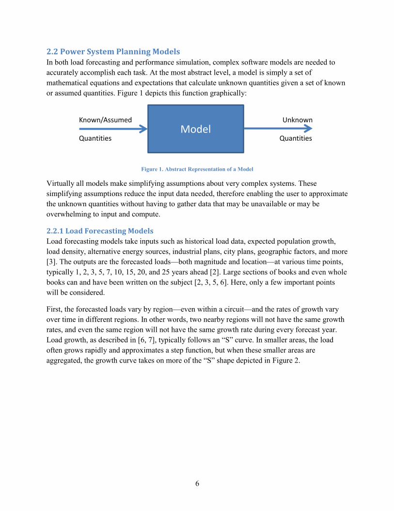
2.2 Power System Planning Models In both load forecasting and performance simulation, complex software models are needed to

accurately accomplish each task. At the most abstract level, a model is simply a set of

mathematical equations and expectations that calculate unknown quantities given a set of known

or assumed quantities. Figure 1 depicts this function graphically:

Figure 1. Abstract Representation of a Model

Virtually all models make simplifying assumptions about very complex systems. These

simplifying assumptions reduce the input data needed, therefore enabling the user to approximate

the unknown quantities without having to gather data that may be unavailable or may be

overwhelming to input and compute.

2.2.1 Load Forecasting Models

Load forecasting models take inputs such as historical load data, expected population growth,

load density, alternative energy sources, industrial plans, city plans, geographic factors, and more

[3]. The outputs are the forecasted loads—both magnitude and location—at various time points,

typically 1, 2, 3, 5, 7, 10, 15, 20, and 25 years ahead [2]. Large sections of books and even whole

books can and have been written on the subject [2, 3, 5, 6]. Here, only a few important points

will be considered.

First, the forecasted loads vary by region—even within a circuit—and the rates of growth vary

over time in different regions. In other words, two nearby regions will not have the same growth

rates, and even the same region will not have the same growth rate during every forecast year.

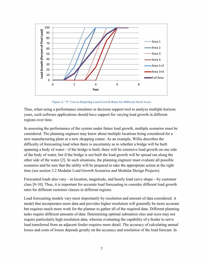
Load growth, as described in [6, 7], typically follows an “S” curve. In smaller areas, the load

often grows rapidly and approximates a step function, but when these smaller areas are

aggregated, the growth curve takes on more of the “S” shape depicted in Figure 2.

Model Known/Assumed Unknown

Quantities Quantities

7

Figure 2. "S" Curves Depicting Load Growth Rates for Different Sized Areas

Thus, when using a performance simulator or decision support tool to analyze multiple horizon

years, such software applications should have support for varying load growth in different

regions over time.

In assessing the performance of the system under future load growth, multiple scenarios must be

considered. The planning engineer may know about multiple locations being considered for a

new manufacturing plant or a new shopping center. As an example, Willis describes the

difficulty of forecasting load when there is uncertainty as to whether a bridge will be built

spanning a body of water—if the bridge is built, there will be extensive load growth on one side

of the body of water, but if the bridge is not built the load growth will be spread out along the

other side of the water [2]. In such situations, the planning engineer must evaluate all possible

scenarios and be sure that the utility will be prepared to take the appropriate action at the right

time (see section 3.2 Modular Load Growth Scenarios and Modular Design Projects).

Forecasted loads also vary—in location, magnitude, and hourly load curve shape—by customer

class [8-10]. Thus, it is important for accurate load forecasting to consider different load growth

rates for different customer classes in different regions.

Load forecasting models vary most importantly by resolution and amount of data considered. A

model that incorporates more data and provides higher resolution will generally be more accurate

but requires much more work for the planner to gather all of the required data. Different planning

tasks require different amounts of data. Determining optimal substation sites and sizes may not

require particularly high resolution data, whereas evaluating the capability of a feeder to serve

load transferred from an adjacent feeder requires more detail. The accuracy of calculating annual

losses and costs of losses depends greatly on the accuracy and resolution of the load forecast. In

0

10

20

30

40

50

60

70

80

90

100

0 2 4 6 8

Load

Gro

wth

(P

erc

en

t o

f Fi

nal

Lo

ad)

Year

Area 1

Area 2

Area 3

Area 4

Area 1+2

Area 3+4

Full Area

8

summary, the planning engineer must use good judgment to evaluate how much accuracy is

required for the task at hand.

2.2.2 Performance Simulation Models

The forecasted load growth then becomes an input into the performance model for evaluating

whether the system will be able to support the forecasted load growth without degrading the

quality of service.

Planning engineers are often familiar with the basic mathematical equations behind performance

simulation models. For a performance simulation model that calculates the voltage drop through

a conductor between an ideal voltage source and a forecasted load, the equations include Ohm’s

law and Kirchoff’s laws, and the known/assumed quantities include the impedance and length of

the conductor, the real (and sometimes reactive) components of the load, and the substation

voltage, as well as an assumption regarding whether the load is modeled as constant power,

constant current, or constant impedance.

Before the advent of computers that could quickly solve large systems of equations, engineers

still used models. Sometimes they might hand-calculate the equations, but, quite often, they had

lookup tables that might contain rules of thumb such as “in conductor X, the voltage will drop by

approximately 0.2% per mile per MW of load.” Such a model was itself derived from

computations using Ohm’s law and Kirchoff’s laws as well as certain assumptions about the

spread of load along the conductor. For the first several decades of power system planning, these

kinds of tables formed the basis for the planning engineer’s decisions regarding how to support

the forecasted load. The models were often conservative, leading to costly, overbuilt systems, but

they provided the desired service level at a cost that was, if not optimal, still affordable to

customers. With modern technology, models can be far more accurate, so systems can be built

that meet the technical requirements with less excess capacity and therefore lower cost.

While balanced three-phase load flow algorithms and even DC load flow algorithms may be

acceptable for transmission planning, optimal distribution level planning generally requires

analysis of unbalanced load flows [2]. Nevertheless, even as late as 2008, some optimization

algorithms still use a DC load flow for faster calculation [11]. Others, such as [12], take

advantage of popular industry software such as PSS/E® for analysis, which limits them to

balanced three-phase load flow calculations. As computers progress and researchers feel the need

to improve upon past work, more and more software applications model three distinct phases,

both for load flow and for short-circuit calculations, such as in [13]. Not only should three

distinct phases be modeled, but the mutual impedances between those phases should be modeled

for more accurate calculations of voltage drop [14].

As indicated earlier, loads can be modeled as constant power, constant current, or constant

impedance, or a combination of the three. While decision support algorithms are mostly limited

to constant power load models, most commercial performance evaluation software, such as

9

ABB’s FeederAll and Electrical Distribution Design’s Distributed Engineering Workstation

allow individual loads to be modeled using any load model [15-17].

Another important aspect of load modeling is the time-varying nature of loads. Many

optimization algorithms only perform peak analysis and then use a load factor to calculate losses

based on the peak. That results in a relatively crude approximation of losses, however, and such

a load model cannot tell the planning engineer such information as how many hours per year a

distributed generator should run or what kind of capacitor control he should use. Alarcon

proposes a “synthetic year” composed of eight 24-hour typical days – one weekday day and one

weekend day for each of the four seasons [18]. Even more important is to distinguish between

the load curves of different classes of customers by using one or more load curves for residential,

commercial, and industrial loads. The monthly kWh sales can then be used to scale those load

curves to more accurately calculate the typical load curve for any type of day in the year. When

hourly load measurements are available, those replace the need for using kWh sales in

conjunction with customer load curves. Once again, it is largely just the commercial software

packages that support more detailed load curve data [15, 19].

Hourly load data for the entire year is really necessary to accurately assess the cost of losses. For

most utilities, not only does the load change continually throughout the year, but the price of

energy changes continually throughout the year. The actual price of energy is determined by the

real-time bidding managed by the regional transmission organization (RTO) or independent

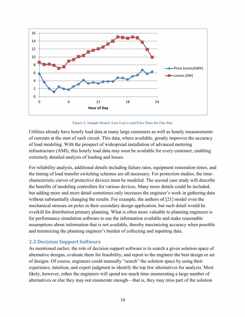
system operator (ISO) and published as the real-time locational marginal price (LMP). Figure 3

below gives a sample plot of losses and locational marginal price for a day in August of 2009,

with pricing data from the New York Independent System Operator [20]. The average price for

the day was $0.0390/kWh, and the average losses per hour were 11.3kWh. The total actual price

of the losses for the day should be calculated by

∑

where is the real power losses for the i

th hour, and is the LMP price at the i

th hour.

Using the formula above, the total actual price of losses is $11.10. Using the average price,

however, results in a cost estimate of $10.57, which is about 5% below the actual price. In order

for a utility to accurately calculate its losses, it needs to use the actual hourly loads and the actual

price.

10

Figure 3. Sample Hourly Loss Curve and Price Data for One Day

Utilities already have hourly load data at many large customers as well as hourly measurements

of currents at the start of each circuit. This data, where available, greatly improves the accuracy

of load modeling. With the prospect of widespread installation of advanced metering

infrastructure (AMI), this hourly load data may soon be available for every customer, enabling

extremely detailed analysis of loading and losses.

For reliability analysis, additional details including failure rates, equipment restoration times, and

the timing of load transfer switching schemes are all necessary. For protection studies, the time-

characteristic curves of protective devices must be modeled. The second case study will describe

the benefits of modeling controllers for various devices. Many more details could be included,

but adding more and more detail sometimes only increases the engineer’s work in gathering data

without substantially changing the results. For example, the authors of [21] model even the

mechanical stresses on poles in their secondary design application, but such detail would be

overkill for distribution primary planning. What is often more valuable to planning engineers is

for performance simulation software to use the information available and make reasonable

assumptions about information that is not available, thereby maximizing accuracy when possible

and minimizing the planning engineer’s burden of collecting and inputting data.

2.3 Decision Support Software As mentioned earlier, the role of decision support software is to search a given solution space of

alternative designs, evaluate them for feasibility, and report to the engineer the best design or set

of designs. Of course, engineers could manually “search” the solution space by using their

experience, intuition, and expert judgment to identify the top few alternatives for analysis. Most

likely, however, either the engineers will spend too much time enumerating a large number of

alternatives or else they may not enumerate enough—that is, they may miss part of the solution

0

2

4

6

8

10

12

14

16

0 6 12 18 24

Hour of Day

Price (cents/kWh)

Losses (kW)

11

space. Of course, software can generate various plans and evaluate them very quickly, but if

there are too many alternatives, the software can take too long as well. Optimization algorithms

attempt to make the search faster and smarter.

Searching the solution space involves not only generating system design configurations but also,

in some optimization algorithms, searching across multiple time horizons. Such methods are

called multi-stage methods and have been developed since at least 1985 [22]. In such algorithms,

the solution space distinguishes between two different time frames for the same system

configurations. The procedures for searching such higher-dimension solution spaces are the same

as for single-horizon planning—only the evaluation becomes more complex and the number of

possible designs in the solution space increases dramatically.

2.3.1 Searching the Solution Space

In some software, the planning engineer may be required to input all designs for evaluation, as in

[12], but, typically, the software generates the alternative designs itself. There are three basic

approaches to automatically searching the solution space of alternative designs:

1. Enumerate all possible alternatives.

2. Search the space using a formal objective function.

3. Search the space using heuristic methods.

Enumerating all possible designs has the advantages of being easy to implement and being

guaranteed to find the optimal solution. For all but the smallest of solution spaces, however,

enumerating and evaluating all possible designs would take far too long.

Formal objective functions “implicitly” search the entire solution space and may have theoretical

proofs of completeness [2]. They do not actually generate every possible design, but at each

iteration they may rule out entire subsets of alternative designs as infeasible or inferior. Willis

strongly favors these optimization algorithms because they are guaranteed not to miss the

optimal solution in their searching. For such algorithms, however, there is no guarantee that the

algorithm will find the optimal solution within a certain time frame. Thus, simplifying

assumptions are often made to speed up the algorithm. For example, although losses are

proportional to the square of the current, they may be linearized to speed up the algorithm [23].

In addition to linear approximations, non-continuous variables (called “integer” variables, even if

they do not always take integer values) are sometimes approximated as continuous variables. For

example, conductors are only available in certain sizes, but the optimization algorithm may

approximate the conductor size as a continuous variable, and, when the algorithm has completed,

the closest available conductor size may be used [24]. Mixed-integer algorithms do not make

such approximations, but therefore require more processing time and thus cannot be used for

solving very large problems. Nevertheless, mixed-integer algorithms have been demonstrated

successfully for decades [22].

12

Heuristic methods can handle much larger problems while guaranteeing that they will produce an

answer in a fixed period of time. They can make such a guarantee because they do not

necessarily search the entire solution space. A heuristic algorithm will start with one or more

designs, and then alter those designs, evaluate the results, and select the best designs from the

new set. At each iteration more alterations are made to the best set from the previous step,

thereby continuing to search the solution space. The heuristic methods can be set to stop at any

iteration—at which point they will simply report the best design or designs found thus far. The

most common types of heuristic methods include simulated annealing, tabu search, and genetic

algorithms, or, sometimes, a combination of all three as in [25]. [26] adds sensitivity analysis-

based algorithms as a separate type of heuristic algorithm. Although heuristic methods are not

guaranteed to find the optimal solution some complexity may be added to broaden the space

searched. For example, in [27] Hadi et al allow some infeasible solutions to persist across

multiple iterations in hopes that, with more alterations in future iterations, some of these

infeasible solutions may produce worthy, feasible solutions. With the advent of multi-core and

multiprocessor computer architectures, heuristic methods have the added advantage of being

naturally suited to parallel computation for even faster execution.

2.3.2 Evaluating Alternatives

At each iteration of an optimization algorithm, the existing design must be evaluated, and the

results of the evaluation determine how the algorithm proceeds during the next iteration. Each

design is typically evaluated first for a violation of one or more constraints to see whether the

design is feasible, and then, if the design is feasible, it is evaluated on the basis of one or more

metrics.

Voltage and thermal limits have long been recognized as the most important constraints in

evaluating whether a design is feasible or not—quite often, in augmentation planning, the reason

for planning is that some piece of equipment will be overloaded in the near future or some

customer will see unacceptably low voltage. Thermal loading limits may also restrict the set of

feasible designs, but in many cases the cost of losses motivates choosing a conductor with a

thermal loading limit two to three times the actual load that will be carried, so an algorithm that

seeks lowest long-term cost will often not contain any heavily-loaded conductors [2]. Voltage,

on the other hand, is very often a limiting constraint. The very first computerized design

application for electric systems used an approximation of voltage drop to check the feasibility of

each solution in its heuristic algorithm [28]. Later, [23] included voltage drop in a formal

optimization algorithm assuming unity power factor, and [22] incorporated voltage drop

calculations based on an input power factor. Both of these algorithms assumed balanced three-

phase loads and flows. More recently, unbalanced load flow has been incorporated into the

optimization algorithms for modeling different voltage drops in different phases, as in, for

example, [13]. Modeling mutual impedances further improves accuracy in modeling voltage

drops for unbalanced loads, as in [14, 29]. In addition to checking for voltage and capacity

13

constraints, some optimization algorithms will check for other constraints, such as checking that

designs do not violate contingency constraints [30].

Once a “feasible” design has been found (or sometimes, even when the design is not feasible, as

in [27]), it must be compared to other designs generated during the current iteration or previous

iterations. Designs may be evaluated for a single criterion or for multiple criteria. If the

evaluation is single-criterion, the criterion is typically cost, and, as long as the computer can

accurately calculate costs, projects may be objectively ranked against one another, and, at the

end of the solution procedure, the lowest-cost design is presented to the user.

If the evaluation involves multiple criteria, the algorithm may take one of two approaches: (1)

convert all criteria to “cost” or (2) produce a non-dominated set of optimal designs, rather than a

single optimal design. Converting all criteria to cost is simple in theory, but difficult in practice.

The only work for the user is to assign a “cost” factor to each criterion. For example, for a utility

with performance-based rates (abbreviated PBR; the utility is paid more for improved reliability

or is penalized for lower reliability), reliability improvements such as SAIDI (system average

interruption duration index) and SAIFI (system average interruption frequency index) can be

assigned a “cost” multiplier based on the performance-based rate. For a utility that simply has

fixed reliability requirements, the “cost” multipliers are somewhat arbitrary. Other criteria may

include voltage and available capacity, which require even more arbitrary “cost” multipliers.

Software applications such as that developed by [13] use this approach to multi-objective

evaluation. While this approach has the benefit of great simplicity, if the arbitrary parameters are

poorly chosen, the results will be skewed toward the multiplier that is too large. For example, if

the reliability “cost” multipliers are varied slightly, the software may alternately choose either an

extremely cheap design with terrible reliability or an extremely expensive solution with great

reliability.

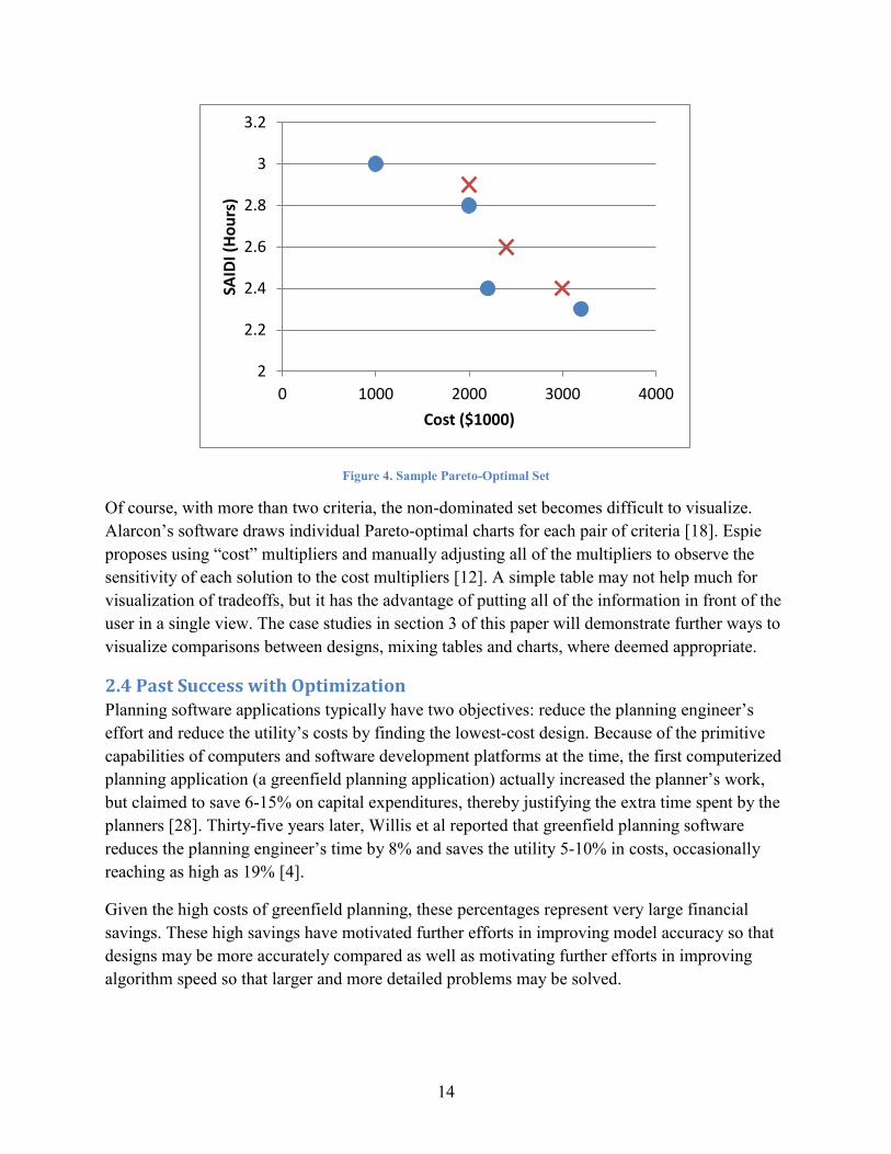
A more popular option for multiple-criteria evaluation is to produce a “non-dominated” set of

alternative designs, and let the planning engineer decide which alternative balances the trade-offs

best. One alternative “dominates” another alternative if it is better in at least one area under

consideration and equal in all other areas of consideration. A non-dominated set of designs for

two criteria form a two-dimensional Pareto-optimal set, as shown in Figure 4 below. The blue

circles represent the non-dominated set of optimal designs, and the red X’s represent dominated

designs. The middle red X is obviously dominated by the third blue circle, since it both costs

more and has lower reliability. Similarly, the top red X is dominated by the second blue circle,

since it costs the same but has worse reliability, whereas the bottom red X is dominated by the

third blue circle, since it has the same reliability but costs more. One might look at the chart and

think that the second blue circle does not belong in the “optimal” set because it represents a very

poor tradeoff between cost and reliability with respect to the first and third circles. Neither the

first nor third circle, however, dominates the second, so this circle does indeed belong in the non-

dominated set. A plot showing the Pareto-optimal set gives the planning engineer a quick visual

depiction of the tradeoffs between cost and reliability.

14

Figure 4. Sample Pareto-Optimal Set

Of course, with more than two criteria, the non-dominated set becomes difficult to visualize.

Alarcon’s software draws individual Pareto-optimal charts for each pair of criteria [18]. Espie

proposes using “cost” multipliers and manually adjusting all of the multipliers to observe the

sensitivity of each solution to the cost multipliers [12]. A simple table may not help much for

visualization of tradeoffs, but it has the advantage of putting all of the information in front of the

user in a single view. The case studies in section 3 of this paper will demonstrate further ways to

visualize comparisons between designs, mixing tables and charts, where deemed appropriate.

2.4 Past Success with Optimization Planning software applications typically have two objectives: reduce the planning engineer’s

effort and reduce the utility’s costs by finding the lowest-cost design. Because of the primitive

capabilities of computers and software development platforms at the time, the first computerized

planning application (a greenfield planning application) actually increased the planner’s work,

but claimed to save 6-15% on capital expenditures, thereby justifying the extra time spent by the

planners [28]. Thirty-five years later, Willis et al reported that greenfield planning software

reduces the planning engineer’s time by 8% and saves the utility 5-10% in costs, occasionally

reaching as high as 19% [4].

Given the high costs of greenfield planning, these percentages represent very large financial

savings. These high savings have motivated further efforts in improving model accuracy so that

designs may be more accurately compared as well as motivating further efforts in improving

algorithm speed so that larger and more detailed problems may be solved.

2

2.2

2.4

2.6

2.8

3

3.2

0 1000 2000 3000 4000

SAID

I (H

ou

rs)

Cost ($1000)

15

The successes in greenfield planning have motivated efforts to develop even better planning

software. In fact, a search in IEEE Xplore of "electrical power distribution planning" returns 600

papers published by the IEEE alone since 2002, nearly all of which describe some new model or

algorithm for finding optimal solutions to either greenfield or augmentation distribution planning

problems (and hundreds more articles may be found on transmission system planning) [31]. Of

course, in order to be worth publishing, the authors typically need to develop software that is

either more advanced or presents some "new" concept. Thus, there has been a marked increase in

the complexity of both the models and algorithms devised for distribution system planning—

both greenfield planning software and augmentation planning software.

After describing the successes of greenfield planning software, however, Willis says,

“Unfortunately, ‘greenfield planning’ represents only a minority of distribution planning needs”

[2]. What is “unfortunate” is that these greenfield software applications cannot be easily

extended to help with the planner’s more common augmentation planning tasks and that

augmentation planning software has not reaped similar benefits. Talking with distribution system

planning engineers today reveals that the same “unfortunate” situation persists today. Today,

planning engineers rarely use any kind of optimization software, and rarely do any performance

simulation beyond load flow analysis and short circuit analysis for one or two alternatives [32,

33]. This is not because there is no augmentation planning software available—of the hundreds

of papers published by the IEEE, many describe software that is only useful in augmentation

planning. Somehow, these software applications have not made the transition from academia to

industry successfully. The next section will attempt to identify some of the deficiencies in

existing planning software while focusing on how planning software might be better developed

in the future to deliver real value to the electric power distribution industry and its engineers.

3. Proposed Planning Software As mentioned above, planning engineers rarely use any kind of optimization software. Instead,

experienced planners often manually determine a solution that they expect to be lowest-cost,

using only the performance simulator that identified the problem and selected based on their

intuition and experience. They may, if the utility requires a comparison of alternatives, manually

devise another solution that they expect to be inferior. Often, they only compare the two

solutions using load flow and perhaps short circuit analysis as well. Typically, when comparing

just the two solutions, they find that their initial expectations were correct, and pursue approval

of the project based on the results of the performance simulator.

A number of factors converge to make this scenario commonplace. The first is that experienced

planners are quite good at identifying the lowest-cost design for remedying problems in system

performance. If the performance simulator and system model are good enough, a planning

engineer facing a circuit with low voltage can relatively quickly and easily see if there is an

obvious phase imbalance, if there is a nearby feeder to which he can transfer load, or if there is

poor power factor which would motivate adding a capacitor. Since each of these projects have

16

widely varying costs, there is no need to compare them all—the planning engineer can start by

looking at feeder transfer capability (the cheapest solution if no new construction is needed),

followed by phase balancing, then capacitor placement, then voltage regulators and distributed

generators, and, if all of these projects prove inadequate, reconductoring or new construction,

stopping once an acceptable solution has been found. Willis said, in warning planning engineers

not to be too confident in their initial expectations, “even the most accomplished planner's initial

intuition about the outcome of a T&D planning study will be wrong about 15% of the time" [2].

That still leaves up to 85% of the time in which experienced planners intuitively know the

optimal or near-optimal solution.

So one must ask, “If planning engineers can quickly find near-optimal solutions through their

own manual work, without using optimization software, is there much value in the optimization

software?” Table 2 summarizes the answer.

Table 2. Computer vs. Human Expertise

Computer Expertise Human Expertise

Generating alternatives from within

a single design category

Generating a variety of alternatives

from different design categories

Computing criteria for

evaluating alternatives

Evaluating alternatives across

multiple criteria, including

assessing trade-offs and risk

A “design category” would be either phase balancing, capacitor placement, reconductoring, or

another type of design. Computers are good at permuting different combinations, given a set of

possible values for each variable. So, for example, given a set of substation locations and a set of

possible transformer sizes, as well as a set of paths for routing conductors and a set of conductor

sizes, a computer can auto-generate designs easily. Similarly, a phase balancing application can

generate all possible phase movements given accurate phasing of conductors and loads.

Computers are not, however, good at generating alternatives from multiple categories of designs.

For example, given a circuit with low voltage somewhere, the computer is not necessarily going

to do a good job of evaluating whether a load transfer, phase balance, voltage regulator,

capacitor, or distributed generator would probably be best. Separate code must be written to

efficiently search each design category’s solution space.

From the bottom row of Table 2, computers are good at calculating metrics, but not necessarily

good at evaluating plans from those metrics, unless, of course, there is only one metric of

importance (e.g. cost). When there are multiple criteria/metrics that cannot be easily converted to

a single metric, the computer is not good at evaluating different options. Since evaluating risk is

increasingly important in the deregulated power distribution industry, human evaluation is

particularly important.

Given the capabilities of software applications described above, one may be surprised that

augmentation planning software has not proven more effective. Willis says, after commenting on

17

the lack of success in augmentation planning software, “The algorithm is still not the key factor

in program usefulness for augmentation applications. The key for augmentation applications is to

make the software usable” [2]. He goes on to say, “A database-editor-display environment

designed to work efficiently with entry, display, and verification of constraints, costs, and the

range of options…provides far greater ease of use” (emphasis his) [2]. In other words, existing

augmentation software has two problems: first, it takes too long to set up the input data to run the

analysis, and, second, augmentation planning applications often don’t support a range of design

categories (such as phase balance, capacitor placement, reconductoring, distributed generation,

etc.). Planning software, then, should provide the following features:

1. System data only needs to be input once, as quickly and easily as possible.

2. Multiple different kinds of independent optimization algorithms can be used with the

same set of system data.

3. The various designs produced by the various optimization algorithms can be brought

together for detailed comparison.

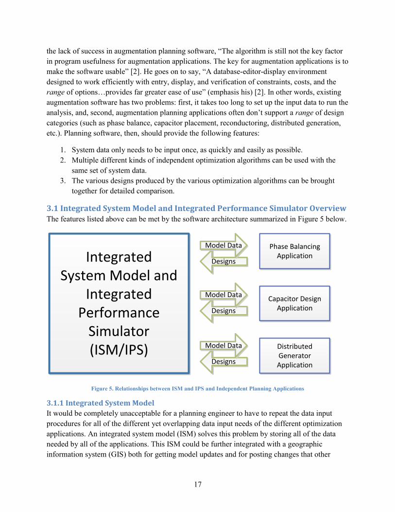
3.1 Integrated System Model and Integrated Performance Simulator Overview The features listed above can be met by the software architecture summarized in Figure 5 below.

IntegratedSystem Model and

Integrated Performance

Simulator(ISM/IPS)

Phase Balancing Application

Capacitor Design Application

Distributed Generator Application

Designs

Model Data

Designs

Model Data

Designs

Model Data

Figure 5. Relationships between ISM and IPS and Independent Planning Applications

3.1.1 Integrated System Model

It would be completely unacceptable for a planning engineer to have to repeat the data input

procedures for all of the different yet overlapping data input needs of the different optimization

applications. An integrated system model (ISM) solves this problem by storing all of the data

needed by all of the applications. This ISM could be further integrated with a geographic

information system (GIS) both for getting model updates and for posting changes that other

18

software applications may need. This integration would be especially helpful for defining right-

of-way information needed for feeder routing, since that information is based on GIS

information.

3.1.2 Independent Optimization Algorithms

It is not surprising that augmentation planning applications don’t support multiple design

categories (e.g. one application doesn’t often analyze both optimal capacitor placement and

optimal phase balancing designs). Different design categories often necessitate different

algorithms for finding the optimal design. For example, a phase balancing application may likely

try all possible phase moves for all single-phase laterals, whereas an optimal capacitor placement

application is not going to consider every single pole in determining capacitor locations.

Similarly, different design categories may have different data input needs. For example, a feeder

routing algorithm requires information like available rights-of-way that are not needed for

distributed generation applications, and distributed generation applications need detailed load

curves, whereas feeder routing algorithms may only need to evaluate performance at peak

(assuming that the load factor is calculated correctly for losses—otherwise, the feeder routing

algorithm also needs detailed load models for calculating losses). Similarly, a capacitor

placement application needs to know what kinds of poles are available for mounting capacitors,

yet a distributed generation application does not need any information about poles. Since these

applications have different data input needs, they also typically have different data input formats.

Since different algorithms must be used for each design category, and since each algorithm has

different data needs, different software applications are generally needed to analyze different

design categories. In order to use these different applications, however, the planning engineer

would have to repeat a lot of work defining the input data for each algorithm. An ISM could

provide a standardized format for accessing needed data of various types. With an ISM, the

planning engineer only has to input the data once and the data becomes available to all planning

applications. Even more importantly, multiple departments in the utility could work together to

maintain the same ISM. Personnel in the “mapping” department could update phasing, while

personnel involved in substation design could update the substation information in the ISM. All

of these updates would become immediately available to every planning application without

requiring further work by the planning engineer.

Not only should the ISM software provide data to individual optimization algorithms, but it

should also have the capability to import the designs generated by those optimization algorithms.

Once the designs have been generated and imported back into the software containing the ISM,

the alternatives may be validated and then evaluated and compared by the planning engineer.

3.1.3 Integrated Performance Evaluator

The comparison described above would take place on an integrated performance simulator (IPS)

application which utilizes all of the model information stored in the ISM.

19

At this point it is worth highlighting that the ISM and IPS need to model at least as many details

as all of the design applications combined, if not more. The IPS should support all of the model

details described in section 2.2.2, including modeling unbalanced power flow and mutual

impedance, as well as such load data as detailed customer load curves, the ability to model loads

as constant power, constant current, or constant impedance, and storage of hourly meter data

where available.

The IPS and ISM also need all of the output data from the load forecasting application, including

variations by year, by customer class, and by location, as described in section 2.2.1.

Additionally, due to the continual improvements in technological capabilities and continual

reduction in costs of advanced technology, the IPS should be able to model real-time control

devices and systems.

Details related to reliability analysis are even more important, even if typical industry values are

used rather than the specific utility’s recorded data. Since deregulation, reliability has become

increasingly important to power system planning, and no two designs should be compared

without considering their relative impacts on reliability.

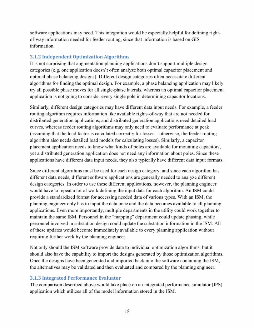
3.2 Modular Load Growth Scenarios and Modular Design Projects Since multiple projects may be required to meet a certain goal, and since one project may greatly

affect the evaluation of another project, it is essential to be able to compare multiple projects

together. These projects must therefore be modular—the design itself, as a series of

modifications to the “base” ISM should be saved independent of the ISM in such a way that

multiple non-conflicting designs may be loaded and “applied” to the ISM in any order.

Similarly, engineers need to evaluate their designs under multiple load forecast scenarios (see

section 2.2.1 Load Forecasting Models). These load forecast scenarios should similarly be

modular, so that they can be loaded with any series of modular designs.

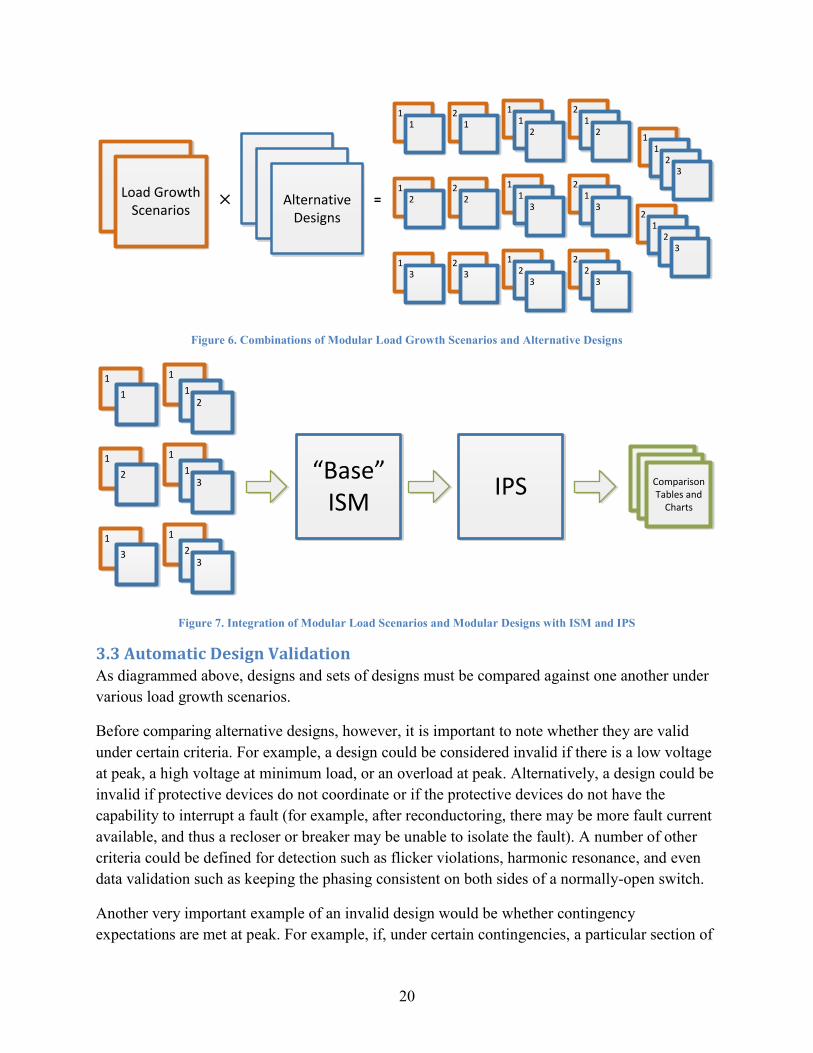
The combination of modular designs and modular load growth scenarios and their relationships

to the ISM and IPS are depicted in Figures 6 and 7 below.

20

Load GrowthScenarios

AlternativeDesigns

11

11

21

12

⨉ =

2

2

3

3

11

21

12

22

13

23

3

21

21

22

2

3

3

11

23

Figure 6. Combinations of Modular Load Growth Scenarios and Alternative Designs

“Base”ISM

Comparison Tables and

Charts

1

1

1

1

1

2

2

3

3

1

1

1

2

1

3

IPS

Figure 7. Integration of Modular Load Scenarios and Modular Designs with ISM and IPS

3.3 Automatic Design Validation As diagrammed above, designs and sets of designs must be compared against one another under

various load growth scenarios.

Before comparing alternative designs, however, it is important to note whether they are valid

under certain criteria. For example, a design could be considered invalid if there is a low voltage

at peak, a high voltage at minimum load, or an overload at peak. Alternatively, a design could be

invalid if protective devices do not coordinate or if the protective devices do not have the

capability to interrupt a fault (for example, after reconductoring, there may be more fault current

available, and thus a recloser or breaker may be unable to isolate the fault). A number of other

criteria could be defined for detection such as flicker violations, harmonic resonance, and even

data validation such as keeping the phasing consistent on both sides of a normally-open switch.

Another very important example of an invalid design would be whether contingency

expectations are met at peak. For example, if, under certain contingencies, a particular section of

21

an adjacent feeder is to be transferred to the feeder under study, then the feeder under study

should be able to support that load. A design change that prevents the feeder from supporting the

load from the adjacent feeder is inferior to a design which supports such switching under

contingencies.

In order to evaluate contingency capability, not only the designs themselves but also the

expected switching operations should be saved as modular items that may be applied to the

“base” ISM to simulate a contingency under the new design.

All of the appropriate validation routines could be set up to run automatically. This would

provide great immediate value to utilities and planning engineers—even if the planning

engineers had to create designs manually. In conversations with utility planning engineers,

switching studies are often neglected by planning engineers. Separate personnel in an operations

department may then be assigned the task of periodically checking switching plans to see

whether they will be valid. Automating this process would provide great value to operations

personnel in addition to helping planning engineers achieve better reliability.

It is important to note that invalid plans may still be compared to valid plans. Comparing the

performance of an invalid plan may still help the planning engineer gain significant insight into

the problem and potential solutions. Furthermore, a planning engineer may decide that it is worth

sacrificing contingency capability at peak for a lower-cost design. He must, however, then alert

operations personnel of the limits of the switching plans.

3.4 Intuitive Visualization of Multiple, Multi-dimensional Criteria H. Lee Willis writes, “A seldom-realized benefit of optimization is that it contributes greatly to

an engineer's understanding of the system and the interplay of costs, performance, and tradeoffs

within it” [4]. That is, by considering multiple alternatives—both multiple alternatives within a

single design category and multiple alternatives across multiple design categories—the engineer

learns about the effectiveness of different designs as well as the sensitivity of the system’s

performance to changes in designs. The engineer gains more understanding—especially of the

tradeoffs involved—when he is able to evaluate and compare more criteria.

Since the deregulation of the electric power industry, nearly every company has faced either

stricter reliability requirements or economic incentives to improve reliability. Thus, all plans

must be compared on the basis of at least two criteria—cost and reliability.

Additionally, utilities are operating their systems closer to the device ratings. Combined with

more emphasis on short-term planning and short-term spending reduction, these operating

conditions require the planning engineer to consider remaining capacity and voltage margins in

evaluating plans. Willis says, “Load reach is both a constraint and a target” (emphasis his) [2].

Load reach is a target insofar as the planning engineer wants the feeder to be able to support

additional load growth beyond the immediate planning horizon but does not want to have to pay

any more up front to acquire such capability. Case Study 1 provides an example where the

22

planning engineer may want to consider voltage (load reach) to be a target, not merely a

constraint.

The integrated performance simulator, therefore, must display information about operating cost

(especially losses), reliability, voltage, available capacity, and more in a way that allows the

planning engineer to easily and intuitively compare multiple designs across multiple criteria. In

addition to supporting multiple-criteria comparisons, the IPS should also help the engineer

compare multi-dimensional criteria. When comparing voltage, for example, the engineer may be

interested to know the lowest voltage at peak for each plan. Such information would give a rather

incomplete comparison of the voltage profile for each circuit. It would be better for the planning

engineer to be able to visually compare the voltage levels around the entire circuit. One option is

to graphically color the circuit by voltage. In order to compare two designs, the performance

simulator could draw two copies of the circuit, each colored by voltage, with one copy

representing one design and the other copy representing the other design. For larger circuits,

however, that would require too much panning and zooming for detailed comparison, and the

engineer may overlook an area of difference. Another valuable approach to comparing voltage

profiles is demonstrated in Case Study 1 and Figure 10, where the numbers of components in

each voltage range are plotted for each design.

In addition to voltage, transformer capacity is a multi-dimensional criterion. As Willis says,

“There is no firm ‘rating’ above which a wound device like a transformer, motor, or regulator

cannot be loaded, at least briefly” [2]. Both the magnitude of the overload and the duration of the

overload are important. Transformer overload evaluation is most important in evaluating

substation contingency capabilities. When one transformer is lost at a substation, the load

normally supplied to that transformer is transferred to one or more transformers at the same

substation or nearby substations. When such transfers are made, the adjacent transformers may

be overloaded. By analyzing the expected outage duration and load curve for a peak day, the

performance simulator can tell the engineer both the magnitude and duration of the expected

overload. Examples of such plots, while not evaluating substation transformer loading, are

shown in Case Study 3 in Figures 15 and 18.

Similarly, reliability may have multiple dimensions—utilities are required not only to meet a

certain average SAIDI requirement but also to ensure that individual customers do not

experience particularly terrible reliability. Thus, in a manner similar to the voltage profile plot

shown in Figure 10 of Case Study 1, the expected interruption durations may be grouped into

ranges and the number of customers in each range may be plotted for various alternative designs

and various alternative load growth scenarios.

3.5 Open Architecture for Performance Simulators

Another feature that could quicken the development of power system planning software would

be the availability of integrated performance simulators built with “open architectures” that

implement standard APIs for executing performance simulations. If the performance evaluator

23

had an “open architecture” then the optimization algorithms could be direct plug-ins to the

performance evaluator, getting ISM data through application programmer interfaces (APIs) as

well as running performance simulation algorithms such as load flow and short circuit

calculations using additional APIs [34]. In addition to sharing APIs for manipulating the model

and sharing some performance simulation algorithms, certain parts of the user-interface

functionality could also be shared, providing a more consistent, user-friendly interface for the

planning engineers using the software.

Such integration of the optimization models with the ISM software is not strictly necessary,

however, and the optimization algorithms may require less-detailed, faster load flow algorithms

anyway. An open architecture would, however, greatly improve reusability and maintainability

of the software suite as a whole, since updates to the load flow algorithm could be made solely in

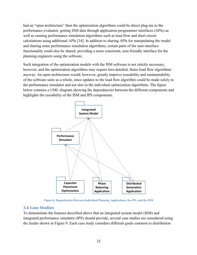
the performance simulator and not also in the individual optimization algorithms. The figure

below contains a UML diagram showing the dependencies between the different components and

highlights the reusability of the ISM and IPS components.

Integrated System Model

Performance Simulator

Capacitor Placement

Optimization

Phase Balancing

Application

Distributed Generation Application

Figure 8. Dependencies Between Individual Planning Applications, the IPS, and the ISM

3.6 Case Studies To demonstrate the features described above that an integrated system model (ISM) and

integrated performance simulator (IPS) should provide, several case studies are considered using

the feeder shown in Figure 9. Each case study considers different goals common to distribution

24

planning (planning for efficiency, planning for voltage requirements, and planning for thermal

loading limits).

The first scenario will highlight the importance of evaluating a feeder’s performance over a full

annual load curve, as well as the need for planning engineers to consider multiple, multi-

dimensional attributes. The second scenario will again demonstrate the value of evaluating a

feeder’s performance over a full annual load curve, as well as highlighting the importance of

analyzing alternate real-time control systems. The third and final scenario will demonstrate the

importance of evaluating multiple loading scenarios (including varying the load growth by

region), as well as the importance of considering distributed energy resources in capacity

planning.

Figure 9 is colored by phase (A is green, B is blue, C is yellow, 3-phase conductors are red, and

the other colors correspond to two-phase conductors). Six locations have been named: M1, M2,

and M3 represent three measurement locations that highlight the phase imbalance throughout the

feeder. Locations NS and WS (“north split” and “west split” for two different three-phase

branches after the “split” after M2) will be used in the capacitor placement case study. ST marks

the location of a step transformer considered in the third case study.

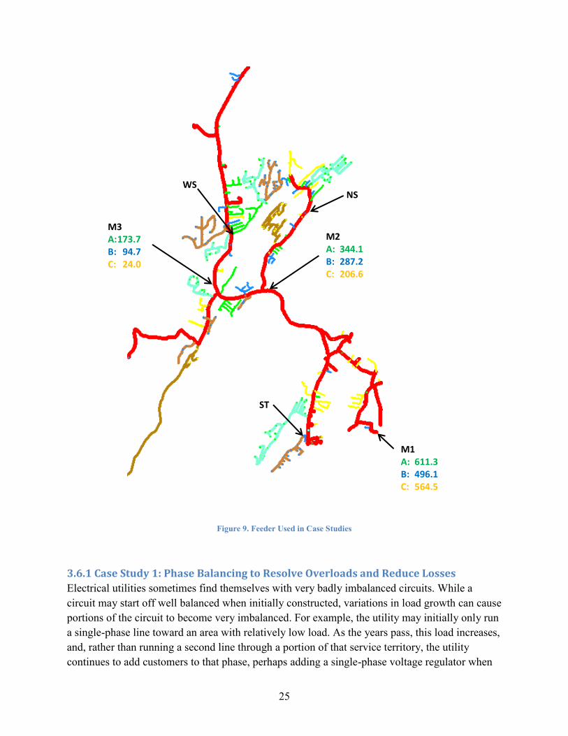
25

Figure 9. Feeder Used in Case Studies

3.6.1 Case Study 1: Phase Balancing to Resolve Overloads and Reduce Losses

Electrical utilities sometimes find themselves with very badly imbalanced circuits. While a

circuit may start off well balanced when initially constructed, variations in load growth can cause

portions of the circuit to become very imbalanced. For example, the utility may initially only run

a single-phase line toward an area with relatively low load. As the years pass, this load increases,

and, rather than running a second line through a portion of that service territory, the utility

continues to add customers to that phase, perhaps adding a single-phase voltage regulator when

M3 A: 173.7 B: 94.7 C: 24.0

M2 A: 344.1 B: 287.2 C: 206.6

M1 A: 611.3 B: 496.1 C: 564.5

NS WS

ST

26

needed to support the voltage along that line. Since losses are proportional to the square of the

current, a single heavily-loaded phase causes exponentially greater losses in all conductors going

all the way back to the source. Simply balancing the currents in the three-phase portions of the

circuit reduces the losses exponentially without reducing the total load power being carried in the

conductors. This phase balancing is accomplished by moving single-phase laterals from one

phase to another where they break from the three-phase trunk.

Furthermore, balancing the phase currents reduces the voltage drops in the more heavily loaded

line, thus potentially resolving voltage issues in the components below it. Even more importantly

to modern distribution planning evaluation, phase balancing is the least expensive manipulation

of the circuit the planning engineer can choose apart from opening and closing switches for load

transfer when available—there is no device to purchase, no need to construct supports on poles

or secure permission to put a box on the ground. The only cost is the crew’s time and the

temporary, scheduled outage. Even if other, more expensive projects are to be done as well, it is

often beneficial to balance the phases first, as the combination may lead to a much better overall

design. For these reasons, phase balancing analysis is often done before other alternative projects

are considered.

In Figure 9, the second measurement (M2) is more than three miles from the start of the circuit

(in the lower-right). At that point, the current on phase A is more than 50% higher than the

current on phase C, partly due to the even larger imbalance further down at location M3. This

imbalance at M2 causes significant losses through those three miles of conductor back to the

substation as well as an overload on a 250kVA voltage regulator (day-to-day rating of 328A)

very close to M2. Additionally, the substation exit cable is getting close to its day-to-day rating

of 649A on phase A because of the imbalance (M1). Notice that, while the phase C current is

very low at the second and third measurement points, the phase C current at the substation exit

cable is larger than the phase B current because of the extra phase C load near the start of the

circuit.

With two phase moves in the upper-left portion of the circuit (in the feed-forward path from

M2), the imbalance at M2 can be greatly reduced, eliminating the overload on the voltage

regulator and greatly reducing the total circuit losses. These phase moves involve moving a

branch on phase A to phase C past the third measurement point (M3) and then moving some load

back from phase C to phase B between M2 and M3. The new phase currents at each

measurement point as well as the total annual losses are summarized in Table 3. The costs of the

annual losses are calculated using LMP data from the New York Independent System Operator

(NYISO) from 2009.

Table 3. Summary of First 2 Phase Balancing Moves

M1 (Amps) M2 (Amps) M3 (Amps) Annual Losses

Before After Before After Before After Before After

Phase A 611.3 546.1 344.1 286.4 173.7 85.7 3.59 GWh 3.54 GWh

27

Phase B 496.1 497.0 287.2 285.8 94.7 94.7 ($168,000) ($166,000)

Phase C 564.5 632.7 206.6 264.6 24.0 112.0

Several points should be noted about the table above. First and most importantly, the phase

imbalance at the start of the circuit got worse. Instead of phase A being exceptionally high, phase

C is now exceptionally high—considerably closer to the substation exit cable’s day-to-day

rating! However, the imbalance favoring phase C is largely due to a lot of single-phase load

close to the start of the circuit. While these loads create an imbalance that almost overloads the

substation exit cable, they do not contribute as much to losses, because the imbalance is in the

first one to two miles of conductor, rather than in the third, fourth, and fifth miles of the

conductor. As will be shown below, further phase balancing operations may reduce the

imbalance at the start of the circuit, but will not affect the losses as significantly.

Second, the voltage regulator at M2 is now safely below its day-to-day rating of 328A.

Third, there is still a noticeable, albeit smaller, imbalance at location M3 (more than 20%). Not

only would the additional work of balancing the currents at M3 be prohibitively expensive, but

the loading may change in future years anyway, causing the imbalance to shift again in

unexpected directions.

Finally, the reduction in losses is so great that the operations pay for themselves in a few years.

Since the conductor at the start of the circuit has a day-to-day rating of 649A, the imbalance

should be corrected again until there is a safer distance between the current on phase C and the

day-to-day rating. At this point, however, the optimal phase move becomes less obvious. There

are many single-phase loads on phase C near the start of the circuit which could be moved to

remedy the problem. Furthermore, the loading on each phase is not uniform throughout the year.

Certain areas may have much more electric load in the winter than others, due, for example, to

heavier reliance on electric heating in certain areas and gas heating in other areas. Not only

might the load concentration change, but the shape of the load curve may change as well. In most

climates, the summer daily load curve for a residential circuit has a single evening peak

occurring after people have arrived home from work, while their air conditioner is still cooling

the house from the heat outside. In winter, residential circuits have two peaks—one peak in the

morning before people leave for work (perhaps, for example, an electric water heater needs to

work harder to supply hot water for showers) and another peak in the evening after people have

returned home but before they go to bed. These two peaks may each be lower than the summer

peak, but, in cooler climates, they may together account for more energy (kWh) consumption

than the summer peak.

In light of these load variations, two alternative phase moves were chosen using an automated

algorithm that makes phase move suggestions based on total feeder losses at selected time points.

To better find the optimal phase move for reducing the losses throughout the entire year, the

algorithm may be run twice—once with each of the following goals:

28

1. Maximize reduction of losses during the summer peak

2. Maximize reduction of losses during the summer and winter peaks

For the first scenario, the peak hour was chosen. For the second scenario, a peak hour in June

and a peak hour in July were chosen for the summer peaks, and a morning peak hour and an

evening peak hour in December were chosen for the winter peaks. (For comparison, the

algorithm was also run for the first day of every month at 7pm and it gave the same answer as the

summer/winter combination). Choosing more time points for analysis occasionally leads to an

answer that further reduces losses, but the analysis then takes proportionally more time to run.

Since the primary goal is to reduce the current on phase C in the substation exit cable, these

currents should be evaluated first, as done in Table 4.

Table 4. Effects of Third Phase Move Options on Substation Exit Cable Currents

Before 3rd

Phase Move

Summer

Phase Move

Summer/Winter

Phase Move

Phase A Current (A) 546.1 545.8 545.1

Phase B Current (A) 497.0 532.5 530.8

Phase C Current (A) 632.7 595.8 598.3

Since they have approximately the same effect on the feeder current and both bring the loading

on the exit cable well below its day-to-day rating, these two alternatives should be compared on

the basis of the total reduction in costs for the entire year. The loss reduction and corresponding

cost reduction (based on LMP data) from each alternative is shown in Table 5.

Table 5. Comparison of Loss Reductions for Each Third Phase Move Option

Summer

Phase Move

Summer/Winter

Phase Move

Annual Loss Reduction 4.5 MWh 6.6 MWh

Value of Loss Reduction $220 $320

Note that the loss reductions above only include the distribution losses—neither the substation

transformer losses nor the transmission losses have been incorporated. Assuming that the

substation transformer is heavily loaded (as it is likely to be, with such a heavily loaded feeder),

the loss reduction in the substation transformer and the transmission system could be comparable

to the loss reduction on the distribution system. Thus, the reduction in losses for the two projects

could actually save closer to $400 and $600 per year, respectively.

Since the choice optimized for both summer and winter peaks saves up to $200 per year more,

one might conclude that the best choice would be to implement the summer/winter phase move

rather than the one based only on the peak loading. In this case, however, the single-objective

evaluation is far from adequate. An important criterion has been left out of the comparison

above: voltage profile.

29

The effects of each alternative on voltage might be compared by simply looking at the lowest

voltage on the circuit. The results are shown in the Table 6 (the voltages with neither phase move

have been included for a more fair comparison—one should always evaluate alternatives against

the existing system).

Table 6. Lowest Voltages On Feeder for Third Phase Move Options

Only Two

Phase Moves

Third

Summer

Phase Move

Third

Summer/Winter

Phase Move

Lowest Customer Voltage, Phase A

(120V base) 112.4 112.2 112.0

Lowest Customer Voltage, Phase B

(120V base) 113.2 112.9 112.2

Lowest Customer Voltage, Phase C

(120V base) 113.6 114.0 113.9

Combining the voltage comparison above with comparison based on the feeder capacity and the

cost of losses, these comparisons form a single-dimension, multiple-attribute design evaluation.

Treating voltage as a single-dimension variable, however, does not always give a fair

comparison of the alternatives. The lowest voltage on the feeder may be at a separate point on

the circuit from the area under consideration, and it may not even be on one of the phases

primarily affected by this project—as in this case—the lowest voltage is on phase A, but both

phase moves under consideration involve moving load from phase C to phase B. Furthermore,

correcting the lowest voltage may require a voltage regulator or capacitor as an additional project

separate from the current design problem, which, in this case, is primarily concerned with the

capacity constraint on the substation exit cable. Since phase balancing should typically be done

before other projects (as explained earlier), one should not be surprised that violations of voltage

constraints persist after phase balancing. A chart such as that shown in Figure 10 better

demonstrates the impact on voltage profile of each of the phase balances considered above.

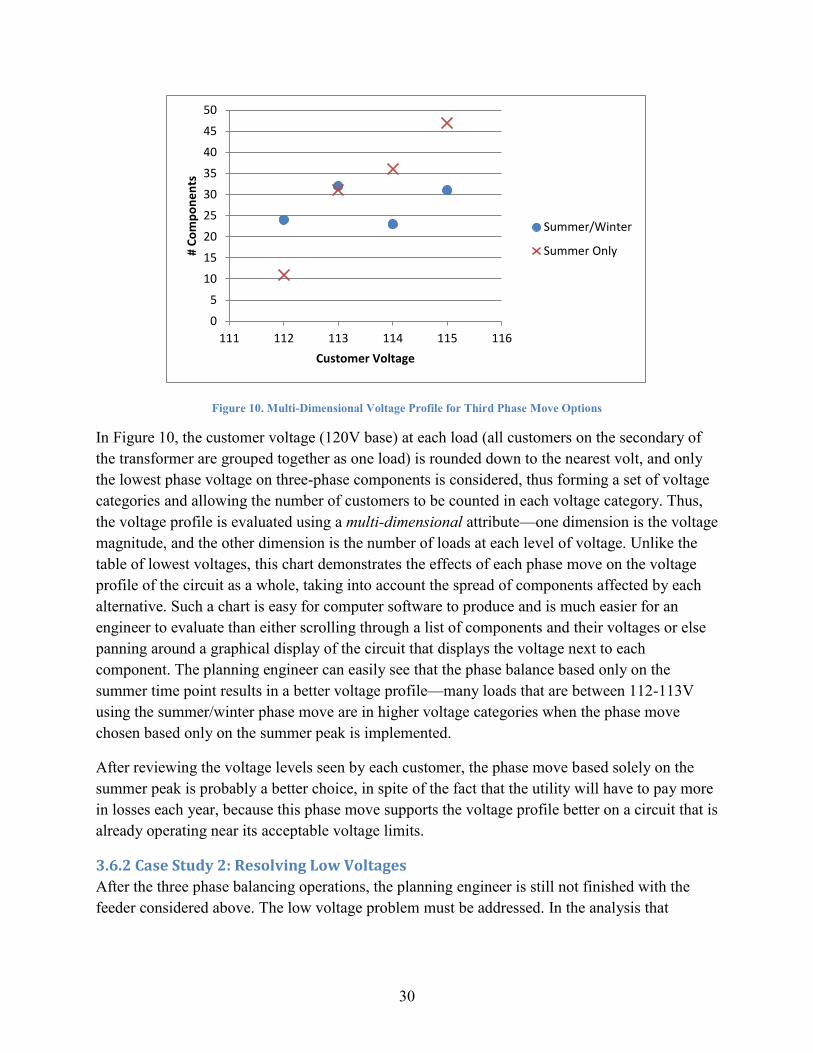
30

Figure 10. Multi-Dimensional Voltage Profile for Third Phase Move Options

In Figure 10, the customer voltage (120V base) at each load (all customers on the secondary of

the transformer are grouped together as one load) is rounded down to the nearest volt, and only

the lowest phase voltage on three-phase components is considered, thus forming a set of voltage

categories and allowing the number of customers to be counted in each voltage category. Thus,

the voltage profile is evaluated using a multi-dimensional attribute—one dimension is the voltage

magnitude, and the other dimension is the number of loads at each level of voltage. Unlike the

table of lowest voltages, this chart demonstrates the effects of each phase move on the voltage

profile of the circuit as a whole, taking into account the spread of components affected by each

alternative. Such a chart is easy for computer software to produce and is much easier for an

engineer to evaluate than either scrolling through a list of components and their voltages or else

panning around a graphical display of the circuit that displays the voltage next to each

component. The planning engineer can easily see that the phase balance based only on the

summer time point results in a better voltage profile—many loads that are between 112-113V

using the summer/winter phase move are in higher voltage categories when the phase move

chosen based only on the summer peak is implemented.

After reviewing the voltage levels seen by each customer, the phase move based solely on the

summer peak is probably a better choice, in spite of the fact that the utility will have to pay more

in losses each year, because this phase move supports the voltage profile better on a circuit that is

already operating near its acceptable voltage limits.

3.6.2 Case Study 2: Resolving Low Voltages

After the three phase balancing operations, the planning engineer is still not finished with the

feeder considered above. The low voltage problem must be addressed. In the analysis that

0

5

10

15

20

25

30

35

40

45

50

111 112 113 114 115 116

# C

om

po

ne

nts

Customer Voltage

Summer/Winter

Summer Only

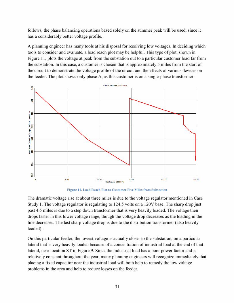
31

follows, the phase balancing operations based solely on the summer peak will be used, since it

has a considerably better voltage profile.

A planning engineer has many tools at his disposal for resolving low voltages. In deciding which

tools to consider and evaluate, a load reach plot may be helpful. This type of plot, shown in

Figure 11, plots the voltage at peak from the substation out to a particular customer load far from

the substation. In this case, a customer is chosen that is approximately 5 miles from the start of

the circuit to demonstrate the voltage profile of the circuit and the effects of various devices on

the feeder. The plot shows only phase A, as this customer is on a single-phase transformer.

Figure 11. Load Reach Plot to Customer Five Miles from Substation

The dramatic voltage rise at about three miles is due to the voltage regulator mentioned in Case

Study 1. The voltage regulator is regulating to 124.5 volts on a 120V base. The sharp drop just

past 4.5 miles is due to a step down transformer that is very heavily loaded. The voltage then

drops faster in this lower voltage range, though the voltage drop decreases as the loading in the

line decreases. The last sharp voltage drop is due to the distribution transformer (also heavily

loaded).

On this particular feeder, the lowest voltage is actually closer to the substation, on a particular

lateral that is very heavily loaded because of a concentration of industrial load at the end of that

lateral, near location ST in Figure 9. Since the industrial load has a poor power factor and is

relatively constant throughout the year, many planning engineers will recognize immediately that

placing a fixed capacitor near the industrial load will both help to remedy the low voltage

problems in the area and help to reduce losses on the feeder.

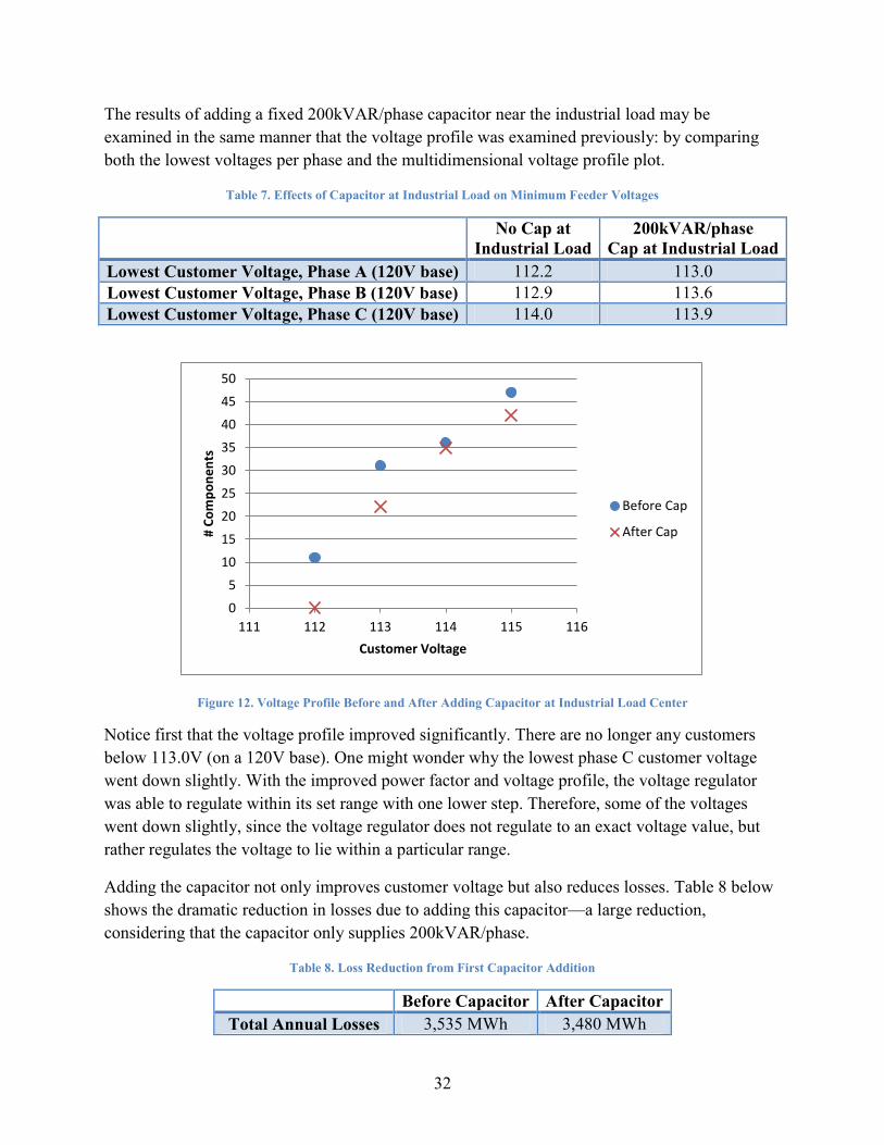
32

The results of adding a fixed 200kVAR/phase capacitor near the industrial load may be

examined in the same manner that the voltage profile was examined previously: by comparing

both the lowest voltages per phase and the multidimensional voltage profile plot.

Table 7. Effects of Capacitor at Industrial Load on Minimum Feeder Voltages

No Cap at

Industrial Load

200kVAR/phase

Cap at Industrial Load

Lowest Customer Voltage, Phase A (120V base) 112.2 113.0

Lowest Customer Voltage, Phase B (120V base) 112.9 113.6

Lowest Customer Voltage, Phase C (120V base) 114.0 113.9

Figure 12. Voltage Profile Before and After Adding Capacitor at Industrial Load Center

Notice first that the voltage profile improved significantly. There are no longer any customers

below 113.0V (on a 120V base). One might wonder why the lowest phase C customer voltage

went down slightly. With the improved power factor and voltage profile, the voltage regulator

was able to regulate within its set range with one lower step. Therefore, some of the voltages

went down slightly, since the voltage regulator does not regulate to an exact voltage value, but

rather regulates the voltage to lie within a particular range.

Adding the capacitor not only improves customer voltage but also reduces losses. Table 8 below

shows the dramatic reduction in losses due to adding this capacitor—a large reduction,

considering that the capacitor only supplies 200kVAR/phase.

Table 8. Loss Reduction from First Capacitor Addition

Before Capacitor After Capacitor

Total Annual Losses 3,535 MWh 3,480 MWh

0

5

10

15

20

25

30

35

40

45

50

111 112 113 114 115 116

# C

om

po

ne

nts

Customer Voltage

Before Cap

After Cap

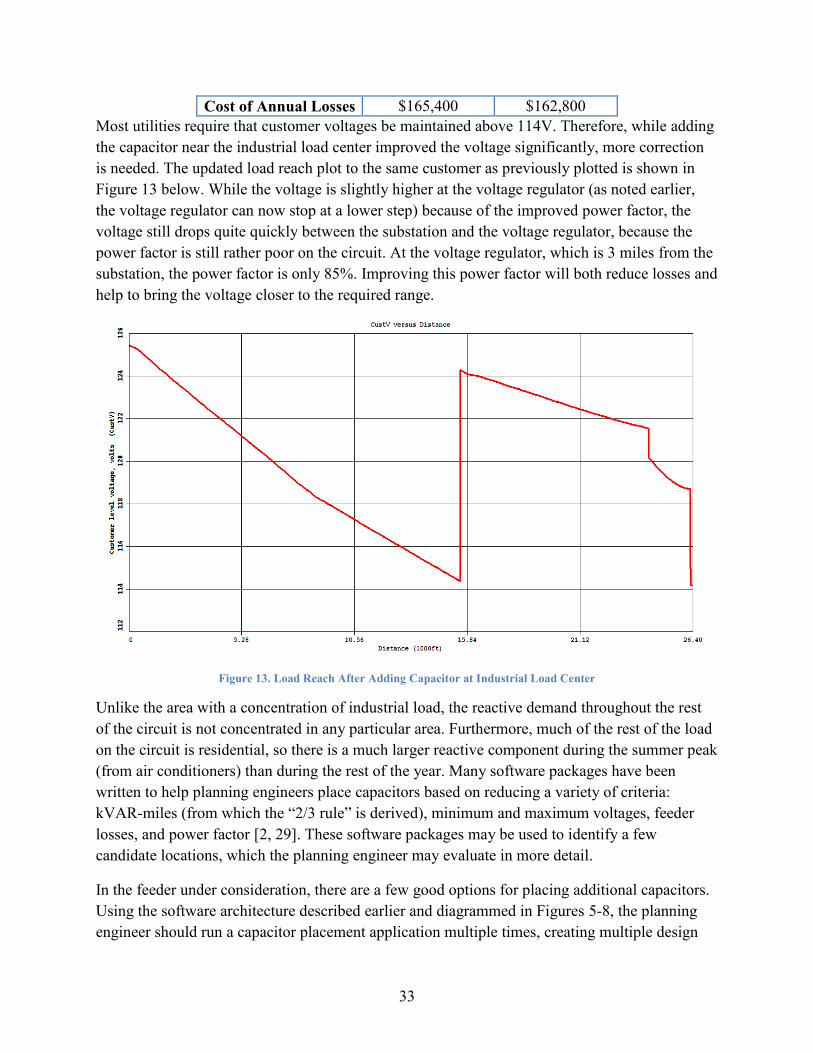
33

Cost of Annual Losses $165,400 $162,800

Most utilities require that customer voltages be maintained above 114V. Therefore, while adding

the capacitor near the industrial load center improved the voltage significantly, more correction

is needed. The updated load reach plot to the same customer as previously plotted is shown in

Figure 13 below. While the voltage is slightly higher at the voltage regulator (as noted earlier,

the voltage regulator can now stop at a lower step) because of the improved power factor, the

voltage still drops quite quickly between the substation and the voltage regulator, because the

power factor is still rather poor on the circuit. At the voltage regulator, which is 3 miles from the

substation, the power factor is only 85%. Improving this power factor will both reduce losses and

help to bring the voltage closer to the required range.

Figure 13. Load Reach After Adding Capacitor at Industrial Load Center

Unlike the area with a concentration of industrial load, the reactive demand throughout the rest

of the circuit is not concentrated in any particular area. Furthermore, much of the rest of the load

on the circuit is residential, so there is a much larger reactive component during the summer peak

(from air conditioners) than during the rest of the year. Many software packages have been

written to help planning engineers place capacitors based on reducing a variety of criteria:

kVAR-miles (from which the “2/3 rule” is derived), minimum and maximum voltages, feeder

losses, and power factor [2, 29]. These software packages may be used to identify a few

candidate locations, which the planning engineer may evaluate in more detail.

In the feeder under consideration, there are a few good options for placing additional capacitors.

Using the software architecture described earlier and diagrammed in Figures 5-8, the planning

engineer should run a capacitor placement application multiple times, creating multiple design

34

projects—one set of projects with a single capacitor and another set of projects with two

capacitors. Perhaps, when optimizing for a single capacitor location, the capacitor placement

application chooses M2, since the lowest voltages all lie before the voltage regulator and are due

to poor power factor and high losses through the three miles of conductor between the substation

and M2, and since placing the capacitor just before the voltage regulator keeps the voltage from

being pushed too high during periods of lighter load. Such placement would still leave

considerable losses at peak past M2. Perhaps, then, when the same application searches for the

optimal two-capacitor placement, it chooses to place capacitors at points NS and WS (NS is

about one mile north of the three-phase split in the main branch just after M2; WS is a mile and a

half past M2 on the westward branch after the split; see Figure 9). Choosing these two locations

would provide excellent voltage support during peak, but these capacitors would need to be

switched off during light-load periods to avoid overvoltage. Using these different locations as

well as possible capacitor sizes ranging from 100kVAR per phase to 400kVAR per phase,

provides a large number of modular designs to be compared. Recall that the output of the

capacitor placement application should consist of modular designs which may be combined in

any way. Thus, for example, in Table 9, configuration 18 would be simply a combination of the

independent, modular configurations 2 and 9.

For the single-capacitor location (M2), a 300kVAR/phase capacitor could be left on year-round,

since the reactive load remains greater than 250 kVAR/phase year-round, and the capacitor

would never cause high voltage, since the voltage regulator would regulate the voltage for

components beyond it. Using a single capacitor that can be left on year-round reduces

maintenance costs, but still leaves a lot of losses past the regulator.

In addition to evaluating the locations, different switching and control schemes must be

evaluated as well. The following control schemes are available to the planning engineer, and

have varying installation and operation costs:

1. Fixed capacitor (never switched off)

a. Lowest capital cost, since no controller is needed

b. Lowest maintenance cost, since it will neither need to be switched, nor will it

wear out quickly

c. Long lifetime, since the capacitor does not move

d. Potentially inefficient—the feeder losses may increase off-peak when the reactive

load is small

2. Capacitor switched manually (switched seasonally)

a. Same capital cost as fixed capacitor

b. Higher maintenance cost, since a crew must be sent to switch the capacitor

seasonally

c. Long lifetime, since the capacitor moves only two or four times per year

d. May be more efficient than fixed capacitor

35

3. Capacitor switched automatically by a local controller (typically switched up to twice per

day)

a. Higher capital cost, due to the cost of installing the controller

b. Moderate maintenance cost, since the capacitor needs to be checked periodically

to make sure that it is switching correctly (due to the lower lifetime discussed

below)

c. Shorter lifetime, since the capacitor switches so frequently

d. More efficient than a manually switched capacitor, since it switches off during

periods of lighter load

4. Capacitor switched by a model-based coordinated control algorithm (switched based on

real-time measurements and performance simulation at a remote control center to

minimize losses and prevent voltage violations)

a. Highest capital cost, due to the communication system needed to gather

measurements and send control signals as well as the development of the software

to operate the devices for optimum performance

b. Low maintenance cost, since the operator knows immediately from the

measurements when the capacitor has switched and when it has failed

c. Lower lifetime, since the capacitor switches more frequently (though the control

algorithm may be calibrated to achieve a desired trade-off between efficiency and

frequency of switching)

d. Most efficient, since the capacitor may be kept consistently in the optimal state

Manual switching is done either twice per year or four times per year (on during summer and

winter and off during spring and fall).

The two most common types of automatic local controllers are time-based controllers and

voltage-based controllers. The time-based controllers switch the capacitors on at the same time

every day and off at the same time every day (these time schedules may be changed seasonally,

or the capacitor may be on a time schedule for the summer and off for the rest of the year).

Voltage controllers will switch the capacitor off when the voltage exceeds a threshold and then

switch it back on when the voltage drops below another, lower threshold (the hysteresis prevents

the capacitor from switching on and off many times for rapidly fluctuating load).

Model-based coordinated control involves remote metering at the capacitor and substation (and

perhaps other available metering locations), with a centralized control software that gathers this

information and analyzes a model of the system to determine the optimal set points.

Having to send a crew to switch a capacitor four times per year could cost up to $800 each year,

depending on the utility’s labor costs and the location of the capacitor (Willis 324). Using a local

controller saves these operating costs, while introducing other costs related to inspection and a

decreased capacitor lifetime. A model-based coordinated control algorithm reduces these

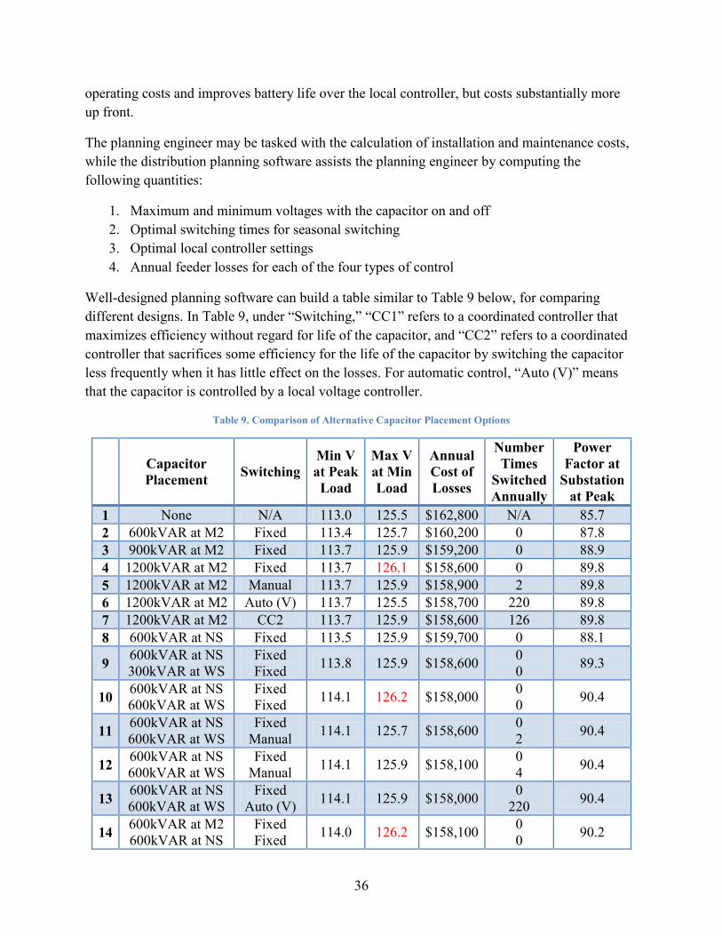
36

operating costs and improves battery life over the local controller, but costs substantially more

up front.

The planning engineer may be tasked with the calculation of installation and maintenance costs,

while the distribution planning software assists the planning engineer by computing the

following quantities:

1. Maximum and minimum voltages with the capacitor on and off

2. Optimal switching times for seasonal switching

3. Optimal local controller settings

4. Annual feeder losses for each of the four types of control

Well-designed planning software can build a table similar to Table 9 below, for comparing

different designs. In Table 9, under “Switching,” “CC1” refers to a coordinated controller that

maximizes efficiency without regard for life of the capacitor, and “CC2” refers to a coordinated

controller that sacrifices some efficiency for the life of the capacitor by switching the capacitor

less frequently when it has little effect on the losses. For automatic control, “Auto (V)” means

that the capacitor is controlled by a local voltage controller.

Table 9. Comparison of Alternative Capacitor Placement Options

Capacitor

Placement Switching

Min V

at Peak

Load

Max V

at Min

Load

Annual

Cost of

Losses

Number

Times

Switched

Annually

Power

Factor at

Substation

at Peak

1 None N/A 113.0 125.5 $162,800 N/A 85.7

2 600kVAR at M2 Fixed 113.4 125.7 $160,200 0 87.8

3 900kVAR at M2 Fixed 113.7 125.9 $159,200 0 88.9

4 1200kVAR at M2 Fixed 113.7 126.1 $158,600 0 89.8

5 1200kVAR at M2 Manual 113.7 125.9 $158,900 2 89.8

6 1200kVAR at M2 Auto (V) 113.7 125.5 $158,700 220 89.8

7 1200kVAR at M2 CC2 113.7 125.9 $158,600 126 89.8

8 600kVAR at NS Fixed 113.5 125.9 $159,700 0 88.1

9 600kVAR at NS

300kVAR at WS

Fixed

Fixed 113.8 125.9 $158,600

0

0 89.3

10 600kVAR at NS

600kVAR at WS

Fixed

Fixed 114.1 126.2 $158,000

0

0 90.4

11 600kVAR at NS

600kVAR at WS

Fixed

Manual 114.1 125.7 $158,600

0

2 90.4

12 600kVAR at NS

600kVAR at WS

Fixed

Manual 114.1 125.9 $158,100

0

4 90.4

13 600kVAR at NS

600kVAR at WS

Fixed

Auto (V) 114.1 125.9 $158,000

0

220 90.4

14 600kVAR at M2

600kVAR at NS

Fixed

Fixed 114.0 126.2 $158,100

0

0 90.2

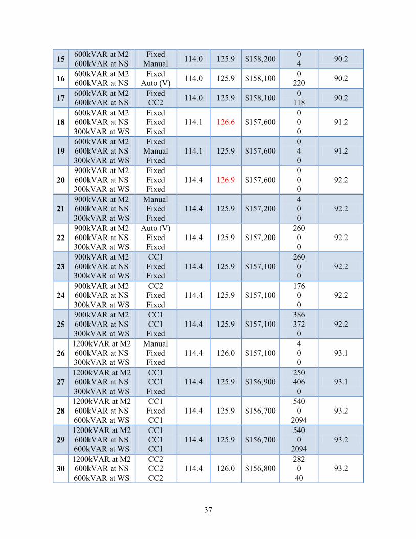
37

15 600kVAR at M2

600kVAR at NS

Fixed

Manual 114.0 125.9 $158,200

0

4 90.2

16 600kVAR at M2

600kVAR at NS

Fixed

Auto (V) 114.0 125.9 $158,100

0

220 90.2

17 600kVAR at M2

600kVAR at NS

Fixed

CC2 114.0 125.9 $158,100

0

118 90.2

18

600kVAR at M2

600kVAR at NS

300kVAR at WS

Fixed

Fixed

Fixed

114.1 126.6 $157,600

0

0

0

91.2

19

600kVAR at M2

600kVAR at NS

300kVAR at WS

Fixed

Manual

Fixed

114.1 125.9 $157,600

0

4

0

91.2

20

900kVAR at M2

600kVAR at NS

300kVAR at WS

Fixed

Fixed

Fixed

114.4 126.9 $157,600

0

0

0

92.2

21

900kVAR at M2

600kVAR at NS

300kVAR at WS

Manual

Fixed

Fixed

114.4 125.9 $157,200

4

0

0

92.2

22

900kVAR at M2

600kVAR at NS

300kVAR at WS

Auto (V)

Fixed

Fixed

114.4 125.9 $157,200

260

0

0

92.2

23

900kVAR at M2

600kVAR at NS

300kVAR at WS

CC1

Fixed

Fixed

114.4 125.9 $157,100

260

0

0

92.2

24

900kVAR at M2

600kVAR at NS

300kVAR at WS

CC2

Fixed

Fixed

114.4 125.9 $157,100

176

0

0

92.2

25

900kVAR at M2

600kVAR at NS

300kVAR at WS

CC1

CC1

Fixed

114.4 125.9 $157,100

386

372

0

92.2

26

1200kVAR at M2

600kVAR at NS

300kVAR at WS

Manual

Fixed

Fixed

114.4 126.0 $157,100

4

0

0

93.1

27

1200kVAR at M2

600kVAR at NS

300kVAR at WS

CC1

CC1

Fixed

114.4 125.9 $156,900

250

406

0

93.1

28

1200kVAR at M2

600kVAR at NS

600kVAR at WS

CC1

Fixed

CC1

114.4 125.9 $156,700

540

0

2094

93.2

29

1200kVAR at M2

600kVAR at NS

600kVAR at WS

CC1

CC1

CC1

114.4 125.9 $156,700

540

0

2094

93.2

30

1200kVAR at M2

600kVAR at NS

600kVAR at WS

CC2

CC2

CC2

114.4 126.0 $156,800

282

0

40

93.2

38

31

1200kVAR at M2

600kVAR at NS

600kVAR at WS

CC2

Fixed

Manual

114.4 126.0 $156,800

282

0

4

93.2

Note that, as before, the losses do not include the substation transformer losses or the

transmission losses, so the actual loss reduction will be even greater.

Although Table 9 includes only a selection of possible arrangements of 300, 600, and

1200kVAR capacitors at the three possible locations with the four possible modes of control, the

table demonstrates many of the tradeoffs planning engineers face when making such decisions.

Comparing the first several rows with various sizes of capacitors at M2 shows the large gains in

efficiency and peak voltage that become possible when the power factor is improved. Comparing

the capacitors at M2 with capacitors at other locations, it is clear that putting the capacitor further

down the feeder reduces losses and improves power factor by a small but noticeable margin—

indicating to the planning engineer that the losses due to poor power factor are significant, even

past the regulator.

Most utilities design their systems to maintain voltages between 114V and 126V, though these

criteria vary by utility. While capacitors help to support voltage during peak by reducing the

current required to supply reactive power, they increase the voltage and losses off-peak when

they back-feed VARs through much of the circuit. Thus, planning engineers frequently find that

they must switch capacitors off during light-load periods to avoid high customer voltages. The

voltages past the regulator will also be highly dependent on the voltage regulator’s movement in

previous hours, since the voltage regulator regulates within a range of voltages, not to a precise

target voltage. For these reasons and since the secondary model may not be perfectly accurate,

the planning engineer may or may not need to act in situations where the estimated maximum

secondary voltage is 126.2V.

Table 9 also shows the kinds of tradeoffs the planning engineer faces when the capacitor must be

switched off during certain parts of the year. In many cases, the capacitor only needs to be

switched off during the very early hours of the morning when the load is at its lowest. Even

during seasons with relatively lower loads, however, the capacitor often helps to reduce losses

during the day when the loads are higher. Since manual switching of the capacitor results in the

capacitor being off during the daytime, which means that the losses may increase slightly during

the months that the capacitor is off. An example can be seen by comparing configurations 4 and

5, where manually switching the 1200kVAR capacitor increases the losses by $300 annually

compared with leaving the capacitor on continuously.

Similarly, the tradeoff between manual control and local control can be seen by comparing

configurations 5 and 6. With the local voltage controller, the capacitor is able to keep the losses

and voltage down by switching on and off 220 times per year. Exchanging the local voltage

controller (6) with a model-based coordinated control algorithm (7) allows the controller to

switch the capacitor less frequently and restore the capacitor sooner, since the software

39

implementing the control algorithm has access to more information than simply a local voltage

measurement. Therefore, the model-based coordinated controller is able to further reduce both

losses and switching cycles, as compared with the local voltage controller.

Although neither a sole 600kVAR capacitor at M2 nor one at NS alone will bring the peak

voltage up into the required range, comparing the two results gives valuable information about

the feeder. The 600kVAR capacitor at NS raised the minimum voltage at peak and reduced the

annual losses more than the 600kVAR capacitor at M2. Since the capacitor is further from the

source, it reduces losses through a greater length of conductor, while also reducing the losses

through the voltage regulator. Putting the 600kVAR capacitor past the voltage regulator,

however, pushed the off-peak voltage to 125.9V. The higher off-peak voltage is not surprising,

since the voltage regulator is already regulating the voltage to a relatively high level, and the

capacitor then further raises the voltage. These tradeoffs are further demonstrated in the

comparison between configurations 3 and 9, where supplying 900kVARs further down the

circuit reduces losses while raising the maximum customer voltages.

Configurations 11 and 12 show a tradeoff between additional manual switching and losses. If the

capacitors are both left on year-round, the voltage will exceed 126.0V during both the spring and

fall. The capacitor could either be switched off at the end of the summer and then switched on

again at the beginning of the next summer (configuration 11), or it could be switched off for a

couple months in the fall and a couple of months in the spring, so that the losses may be reduced

during the higher load periods in winter.

In configuration 18, the planning engineer sees that adding a third capacitor continues to

decrease the losses but puts the maximum voltage far outside an acceptable range. Comparing

with configuration 19, however, shows that almost all of the loss reduction is maintained (to 4

significant digits) even when the capacitor is switched off during part of the spring and fall. In

this case, the losses do not rise because the circuit is actually more efficient during low-load

periods with only the 900kVAR supply than with the additional 600kVARs. Even more so, in

configurations 20 and 21 the cost of losses drops substantially when the 900kVAR capacitor is

switched off twice per year.

When the local controller in configuration 22 is replaced with a model-based controller, the

control algorithm could aggressively switch the capacitor to reduce losses (configuration 23), or

it could sacrifice losses during parts of the year to reduce capacitor switching (configuration 24).

In this case, the less aggressive algorithm increases the losses so little that the reduction does not

show up when only four significant digits are displayed. In fact, configuration 25 shows that

adding an aggressive controller that is allowed to switch both the capacitor at M2 and the

capacitor at NS still does not affect the losses significantly. Similarly, configurations 26 and 27

show that, even with a larger capacitor at M2, the most aggressive switching still does not reduce

the losses by more than about $200 per year, compared with manual switching.

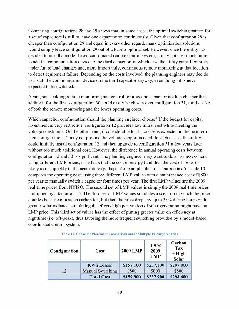
40

Comparing configurations 28 and 29 shows that, in some cases, the optimal switching pattern for

a set of capacitors is still to leave one capacitor on continuously. Given that configuration 28 is

cheaper than configuration 29 and equal in every other regard, many optimization solutions

would simply leave configuration 29 out of a Pareto-optimal set. However, once the utility has

decided to install a model-based coordinated remote control system, it may not cost much more

to add the communication device to the third capacitor, in which case the utility gains flexibility

under future load changes and, more importantly, continuous remote monitoring at that location

to detect equipment failure. Depending on the costs involved, the planning engineer may decide

to install the communication device on the third capacitor anyway, even though it is never

expected to be switched.

Again, since adding remote monitoring and control for a second capacitor is often cheaper than

adding it for the first, configuration 30 could easily be chosen over configuration 31, for the sake

of both the remote monitoring and the lower operating costs.

Which capacitor configuration should the planning engineer choose? If the budget for capital

investment is very restrictive, configuration 12 provides low initial cost while meeting the

voltage constraints. On the other hand, if considerable load increase is expected in the near term,

then configuration 12 may not provide the voltage support needed. In such a case, the utility

could initially install configuration 12 and then upgrade to configuration 31 a few years later

without too much additional cost. However, the difference in annual operating costs between

configuration 12 and 30 is significant. The planning engineer may want to do a risk assessment

using different LMP prices, if he fears that the cost of energy (and thus the cost of losses) is

likely to rise quickly in the near future (perhaps, for example, due to a “carbon tax”). Table 10

compares the operating costs using three different LMP values with a maintenance cost of $800

per year to manually switch a capacitor four times per year. The first LMP values are the 2009

real-time prices from NYISO. The second set of LMP values is simply the 2009 real-time prices

multiplied by a factor of 1.5. The third set of LMP values simulates a scenario in which the price

doubles because of a steep carbon tax, but then the price drops by up to 33% during hours with

greater solar radiance, simulating the effects high penetration of solar generation might have on

LMP price. This third set of values has the effect of putting greater value on efficiency at

nighttime (i.e. off-peak), thus favoring the more frequent switching provided by a model-based

coordinated control system.

Table 10. Capacitor Placement Comparison under Multiple Pricing Scenarios

Configuration Cost 2009 LMP

1.5 ⨉

2009

LMP

Carbon

Tax

+ High

Solar

12

KWh Losses $158,100 $237,100 $297,800

Manual Switching $800 $800 $800

Total Cost $159,900 $237,900 $298,600

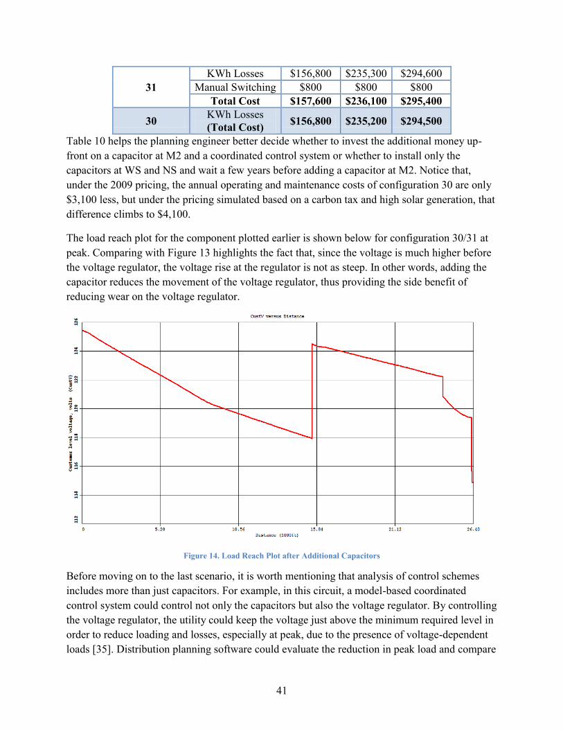
41

31

KWh Losses $156,800 $235,300 $294,600

Manual Switching $800 $800 $800

Total Cost $157,600 $236,100 $295,400

30 KWh Losses

(Total Cost) $156,800 $235,200 $294,500

Table 10 helps the planning engineer better decide whether to invest the additional money up-

front on a capacitor at M2 and a coordinated control system or whether to install only the

capacitors at WS and NS and wait a few years before adding a capacitor at M2. Notice that,

under the 2009 pricing, the annual operating and maintenance costs of configuration 30 are only

$3,100 less, but under the pricing simulated based on a carbon tax and high solar generation, that

difference climbs to $4,100.

The load reach plot for the component plotted earlier is shown below for configuration 30/31 at

peak. Comparing with Figure 13 highlights the fact that, since the voltage is much higher before

the voltage regulator, the voltage rise at the regulator is not as steep. In other words, adding the

capacitor reduces the movement of the voltage regulator, thus providing the side benefit of

reducing wear on the voltage regulator.

Figure 14. Load Reach Plot after Additional Capacitors

Before moving on to the last scenario, it is worth mentioning that analysis of control schemes

includes more than just capacitors. For example, in this circuit, a model-based coordinated

control system could control not only the capacitors but also the voltage regulator. By controlling

the voltage regulator, the utility could keep the voltage just above the minimum required level in

order to reduce loading and losses, especially at peak, due to the presence of voltage-dependent

loads [35]. Distribution planning software could evaluate the reduction in peak load and compare

42

the reduction in sales with the reduction in losses as well as the impact on regulator wear-and-

tear of the control system. Since the marginal cost of adding communication and control

hardware to the regulator is much lower if the communication system is already in place for the

capacitor controls, such a control system could prove to be a very economical way to lower loads

at peak to avoid future capital expenditures.

3.6.3 Case Study 3: Resolving Overloads

Also on the same circuit is a step down transformer that is overloaded at peak (location ST in

Figure 9). Up until about a decade ago, the planning engineer would have had three ways to

resolve the overload: (1) replace the existing step transformer with a bigger step transformer, (2)

transfer a portion of the circuit to an adjacent feeder, or (3) upgrade the voltage class so that no

step transformer is needed. In recent years, utilities have been using distributed energy resources

as alternatives to higher-cost capital investments. Distribution planning software should therefore

calculate and display information pertinent to the use of distributed resources.

While diesel generators can be very inexpensive to install, relative to their large output power, it

is particularly difficult to get siting permission close to residential areas. Thus, since this

overload is in a residential area, battery energy storage (BES) devices will be evaluated as the

distributed resource (distribution planning software should, however, allow the planning

engineer to compare a variety of distributed resources and control algorithms). Placing individual

BES devices at each transformer has the added benefit of vastly improving the reliability of the

electric power supply to the customers fed by those transformers, since the BES device may be

used to supply power in case of an outage by disconnecting the storage device and the secondary

from the power system. The battery storage devices analyzed here store 50 kilowatt-hours each,

and have maximum outputs of 25kW. Thus, they can supply a 25kW load for two hours in case

of an outage when fully charged.

In this case, the load could not be transferred to an adjacent feeder without some additional

construction—again in an area where it will be difficult to obtain the necessary rights-of-way, so

this option will not be considered in this paper, though distribution planning software should

provide a user-friendly interface for drawing in the new construction and evaluating both

affected feeders under various loading conditions. Thus, three options remain for the planning

engineer: (1) upgrading the step transformer from 333kVA to 500kVA, (2) placing BES units on

various transformers, and (3) removing the step down transformer and upgrading the voltage

class.

The most important factor to consider in evaluating the three different design alternatives is cost.

Before the costs are considered, however, the three designs must be evaluated in terms of their

ability to serve the load without overloading equipment or allowing the customer voltage to drop

below 114V on a 120V base.

43

In evaluating these alternatives, it is especially important that the planning engineer consider

future load growth. It would be incredibly costly to replace the step transformer with a larger

step transformer now, only to have to replace that step transformer a few years later due to

additional load growth.

3.6.3.1 Load Growth Scenario 1

The first load growth scenario is shown in Table 11. The “local” residential load growth refers to

the load growth supplied by the step transformer. In the first two years, the local load growth is

higher than the residential growth on the rest of the feeder, because some of the houses on the

market in the area are expected to sell in the next couple of years. In year three, the residential

load growth starts to increase system-wide, due to expectations of increased adoption of plug-in

electric vehicles (PEVs). The sale of PEVs rises even further in year 5 as the technology starts to

mature. The industrial and commercial loads are expected to decrease slightly due to

improvements in energy efficiency.

Table 11. Load Growth Scenario 1

Year # %Res (Local) %Res (All) %Comm %Ind

0 0 0 0 0

1 3 1 0 -2

2 2 1 0 -2

3 1.5 1.5 1 0

4 1.5 1.5 1 0

5 2 2 1 0

6 2 2 1 0

7 2 2 1 0

8 2 2 1 0

In evaluating the option to replace the step transformer with a larger step transformer, the loading

on the new step transformer is very important. Unlike fuses and conductors, transformers do not

have a firm limit on how much current they can support. The loss of transformer life and

probability of failure are functions of both the percent loading and the number of hours that the

transformer is loaded at that level. Thus, like voltage, transformer loading becomes a multi-

dimensional attribute. Figure 15 shows a sample plot of what power distribution planning

software might show to express the multi-dimensional attribute of transformer loading.

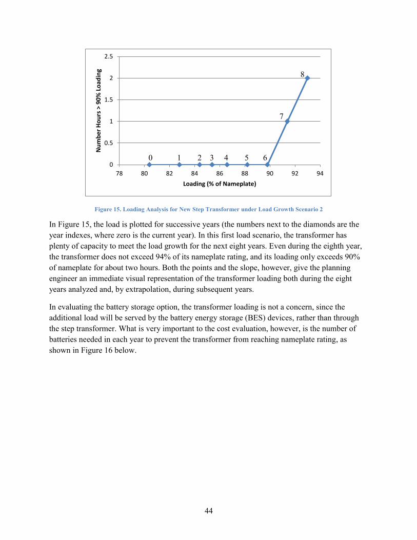
44

Figure 15. Loading Analysis for New Step Transformer under Load Growth Scenario 2

In Figure 15, the load is plotted for successive years (the numbers next to the diamonds are the

year indexes, where zero is the current year). In this first load scenario, the transformer has

plenty of capacity to meet the load growth for the next eight years. Even during the eighth year,

the transformer does not exceed 94% of its nameplate rating, and its loading only exceeds 90%

of nameplate for about two hours. Both the points and the slope, however, give the planning

engineer an immediate visual representation of the transformer loading both during the eight

years analyzed and, by extrapolation, during subsequent years.

In evaluating the battery storage option, the transformer loading is not a concern, since the

additional load will be served by the battery energy storage (BES) devices, rather than through

the step transformer. What is very important to the cost evaluation, however, is the number of

batteries needed in each year to prevent the transformer from reaching nameplate rating, as

shown in Figure 16 below.

0

0.5

1

1.5

2

2.5

78 80 82 84 86 88 90 92 94

Nu

mb

er

Ho

urs

> 9

0%

Lo

adin

g

Loading (% of Nameplate)

0 1 2 3 4 5 6

7

8

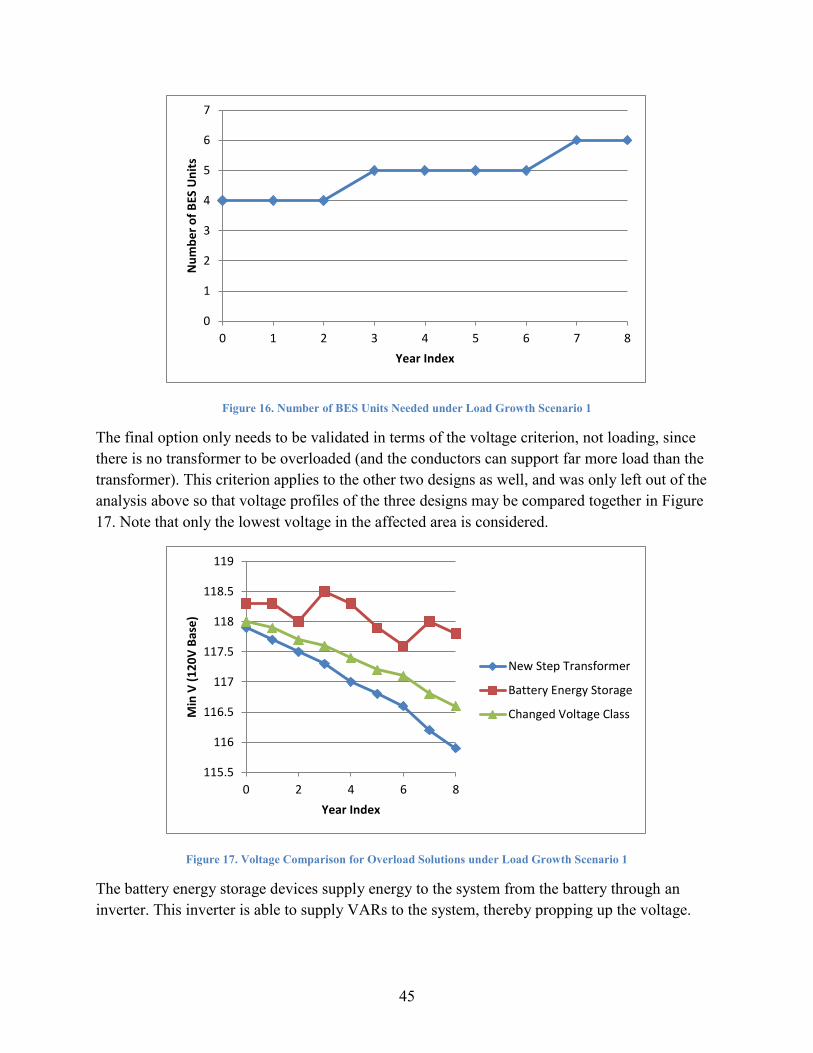
45

Figure 16. Number of BES Units Needed under Load Growth Scenario 1

The final option only needs to be validated in terms of the voltage criterion, not loading, since

there is no transformer to be overloaded (and the conductors can support far more load than the

transformer). This criterion applies to the other two designs as well, and was only left out of the

analysis above so that voltage profiles of the three designs may be compared together in Figure

17. Note that only the lowest voltage in the affected area is considered.

Figure 17. Voltage Comparison for Overload Solutions under Load Growth Scenario 1

The battery energy storage devices supply energy to the system from the battery through an

inverter. This inverter is able to supply VARs to the system, thereby propping up the voltage.

0

1

2

3

4

5

6

7

0 1 2 3 4 5 6 7 8

Nu

mb

er

of

BES

Un

its

Year Index

115.5

116

116.5

117

117.5

118

118.5

119

0 2 4 6 8

Min

V (

12

0V

Bas

e)

Year Index

New Step Transformer

Battery Energy Storage

Changed Voltage Class

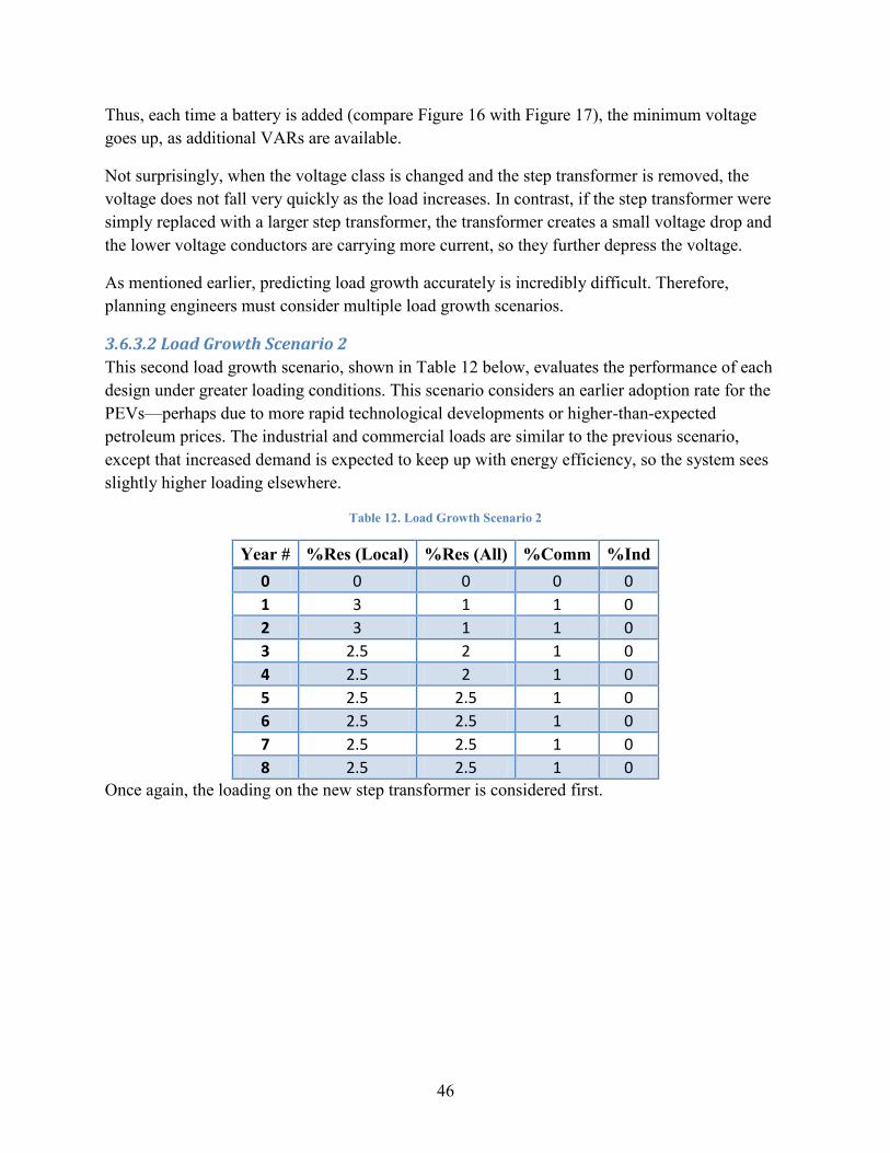
46

Thus, each time a battery is added (compare Figure 16 with Figure 17), the minimum voltage

goes up, as additional VARs are available.

Not surprisingly, when the voltage class is changed and the step transformer is removed, the

voltage does not fall very quickly as the load increases. In contrast, if the step transformer were

simply replaced with a larger step transformer, the transformer creates a small voltage drop and

the lower voltage conductors are carrying more current, so they further depress the voltage.

As mentioned earlier, predicting load growth accurately is incredibly difficult. Therefore,

planning engineers must consider multiple load growth scenarios.

3.6.3.2 Load Growth Scenario 2

This second load growth scenario, shown in Table 12 below, evaluates the performance of each

design under greater loading conditions. This scenario considers an earlier adoption rate for the

PEVs—perhaps due to more rapid technological developments or higher-than-expected

petroleum prices. The industrial and commercial loads are similar to the previous scenario,

except that increased demand is expected to keep up with energy efficiency, so the system sees

slightly higher loading elsewhere.

Table 12. Load Growth Scenario 2

Year # %Res (Local) %Res (All) %Comm %Ind

0 0 0 0 0

1 3 1 1 0

2 3 1 1 0

3 2.5 2 1 0

4 2.5 2 1 0

5 2.5 2.5 1 0

6 2.5 2.5 1 0

7 2.5 2.5 1 0

8 2.5 2.5 1 0

Once again, the loading on the new step transformer is considered first.

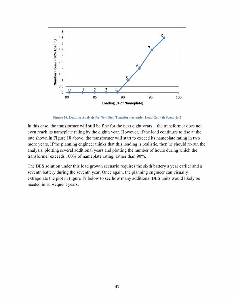
47

Figure 18. Loading Analysis for New Step Transformer under Load Growth Scenario 2

In this case, the transformer will still be fine for the next eight years—the transformer does not

even reach its nameplate rating by the eighth year. However, if the load continues to rise at the

rate shown in Figure 18 above, the transformer will start to exceed its nameplate rating in two

more years. If the planning engineer thinks that this loading is realistic, then he should re-run the

analysis, plotting several additional years and plotting the number of hours during which the

transformer exceeds 100% of nameplate rating, rather than 90%.

The BES solution under this load growth scenario requires the sixth battery a year earlier and a

seventh battery during the seventh year. Once again, the planning engineer can visually

extrapolate the plot in Figure 19 below to see how many additional BES units would likely be

needed in subsequent years.

0

0.5

1

1.5

2

2.5

3

3.5

4

4.5

5

80 85 90 95 100

Nu

mb

er

Ho

urs

> 9

0%

Lo

adin

g

Loading (% of Nameplate)

0 1 2 3 4

5

6

7

8

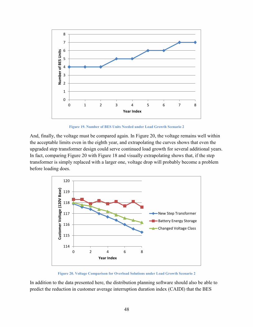
48

Figure 19. Number of BES Units Needed under Load Growth Scenario 2

And, finally, the voltage must be compared again. In Figure 20, the voltage remains well within

the acceptable limits even in the eighth year, and extrapolating the curves shows that even the

upgraded step transformer design could serve continued load growth for several additional years.

In fact, comparing Figure 20 with Figure 18 and visually extrapolating shows that, if the step

transformer is simply replaced with a larger one, voltage drop will probably become a problem

before loading does.

Figure 20. Voltage Comparison for Overload Solutions under Load Growth Scenario 2

In addition to the data presented here, the distribution planning software should also be able to

predict the reduction in customer average interruption duration index (CAIDI) that the BES

0

1

2

3

4

5

6

7

8

0 1 2 3 4 5 6 7 8

Nu

mb

er

of

BES

Un

its

Year Index

114

115

116

117

118

119

120

0 2 4 6 8

Cu

sto

me

r V

olt

age

(1

20

V B

ase

)

Year Index

New Step Transformer

Battery Energy Storage

Changed Voltage Class

49

solution would provide. The higher cost of the BES solution, in comparison with replacing the

step transformer, would probably only make sense if the utility received a considerable benefit

from the improved reliability.

The final decision must be left to the planning engineer. The performance evaluation performed

above, in combination with a reliability analysis, enables the engineer to evaluate the tradeoffs in

cost (both near-term and long-term) and reliability to determine the best option.

3.6.4 Case Study Conclusions

Each case study demonstrates a different feature that the ISM and IPS should provide to the

planning engineer to help him make better decisions. The first case study demonstrated that

evaluating multiple criteria (in this case voltage and cost) sometimes leads to a better design

decision than examining a single variable (such as cost) alone. Furthermore, the first case study

demonstrates the importance of looking at voltage as a multi-dimensional criterion, rather than as

a single-dimensional criterion.

The second case study demonstrates the importance of being able to model the impacts on feeder

performance of different real-time control systems. As technology improves and the cost of

advanced communication and control systems decreases, planning engineers will be looking

more and more to the control systems to help operate the system at maximum efficiency and

closer to operating constraints.

The third case study demonstrates the importance of running multiple loading scenarios, as well

as varying the load growth by region. The case study also highlights the relevance of evaluating

distributed energy resources as alternatives to more expensive capital investments.

Of course, in situations as described above, when the analysis successively resolves different

problems on a single feeder, earlier design choices should be re-evaluated with the later design

choices. In this case, the choice of the third phase move from Case Study 1 should be re-

evaluated with the capacitors as chosen in the second case study, since the capacitors may reduce

the need for the better voltage support provided by the phase balance chosen in the first case

study. Even more importantly, if battery storage devices are used to reduce peak loading on a

single phase, as in the third case study, then that could significantly affect the optimal phase

balance choice – perhaps even more load should be moved to phase B (the step transformer was

a single-phase transformer on phase B). Similarly, though probably with less benefit, the

capacitor study should be re-done with the battery storage devices, since the inverters also

provide VARs. These additional scenarios demonstrate the importance of storing design projects

and loading scenarios as separate, modular components which may be combined in any order for

analysis. Even the LMP pricing should be modular, as demonstrated in the second case study.

50

4. Conclusions, Contributions, and Future Work

4.1 Conclusions and Contributions

The goal of electric power system planning is to ensure that the system serves its load reliably

within certain technical specifications at lowest long-term cost. Uncertainty in both the

magnitude and location of future load growth greatly complicates the planning task, as do the

wide variety of social, political, environmental, technological, and economic factors which affect

the cost and variety of options available to the planning engineer.

A great number of sophisticated models have been developed to assist the planning engineer in

thoroughly evaluating the performance of the system under various conditions. Likewise, a great

number of sophisticated algorithms have been developed to assist the planning engineer in

finding optimum designs within different solution spaces to serve the expected loads.

These algorithms have been quite successful in helping planning engineers lay out feeders and

plan substation expansion—planning activities often called greenfield planning because they

help the planner determine how to serve yet undeveloped (“green”) areas. A more common

planning activity, called augmentation planning, involves making modifications to the existing

system due to load growth in already developed areas. In this latter form of planning, the

decision support software has not generally served planning engineers very well. This work sets

out both to identify some of the reasons that these software applications have not made the

transition from academia to industry and to identify some software architecture considerations

that would facilitate the use of more software applications in augmentation planning.

Three reasons were identified that keep augmentation planning applications from being used

more widely in industry: (1) different design categories require different software applications,

(2) these different applications require different data, often in different formats, and (3) planning

engineers do not have an easy way to compare the results of these different planning

applications.

The following features have been identified to facilitate greater use of a variety of planning

applications: an integrated system model (ISM), an integrated performance simulator (IPS),

modular design projects and load growth scenarios, and visualization of multiple, multi-

dimensional criteria.

An integrated system model (ISM) provides a centralized approach to storing the various data as

well as a standard format and standard set of application programmer interfaces (APIs) for

getting the data needed, as diagrammed in Figure 5. If each optimization algorithm could get its

data from the ISM, the planning engineer would be able to run a much wider variety of

applications for different kinds of design categories without having to gather and format data

independently for each application.

51

Moreover, once the individual augmentation planning applications have been run, their designs

must be thoroughly compared across a wide variety of criteria under a variety of potential load

growth scenarios. The architecture suggested in this paper utilizes an integrated performance

simulator (IPS) for comparing modular design projects under modular load growth scenarios, as

diagrammed in Figure 7. In addition to performing a very detailed analysis for the engineer to

evaluate and compare the alternatives, the IPS can automatically run any number of validation

routines on a given design or set of designs to alert the planning engineer of operating problems

or additional equipment and planning needs that may not have been anticipated.

In order to facilitate comparison of the various designs generated by the individual optimization

algorithms, the IPS must be able to not only compute a great number of metrics but also present

those metrics in a visually accessible way. To help the planning engineer understand the various

trade-offs between alternative designs, the IPS should provide intuitive visualization of multiple,

multi-dimensional criteria.

This work provides three case studies which demonstrate the kinds of detailed evaluation and

comparison that an IPS could facilitate. Throughout the case studies, many figures and tables

demonstrate various ways that multiple, multi-dimensional criteria could be visualized to help

the planning engineer evaluate designs and understand the trade-offs involved in each design

decision. The case studies further highlight the importance of being able to generate and analyze

a set of modular designs and load growth scenarios which may be combined together in various

ways, as diagrammed in Figure 6, to help the planning engineer understand the effectiveness of

various combinations of designs under various load growth scenarios.

4.2 Future Work In the case studies examined here, many cost and risk analysis details were left out. Planning

engineers face a large variety of costs as well as much uncertainty regarding certain types of

costs. Most planning engineers already have electronic spreadsheet programs for evaluating costs

as well as risk. While the IPS could incorporate these cost factors into its comparison routines,

the planning engineer would face at least as much work in entering the cost data into the IPS

software as in entering the cost data into an electronic spreadsheet. Thus, the planning engineer

would further lose flexibility in incorporating additional cost categories into the analysis if the

IPS did not anticipate those cost categories.

Incorporating cost and risk analysis into the IPS software could, however, help the planning

engineer in several ways. First, the IPS software could guard against mistakes in formulas

entered into a spreadsheet. Second, the IPS software could standardize the cost data to ensure

that the planning engineer does not leave out any important factors and to further ensure that all

planning engineers are evaluating plans consistently across the utility. Further research would be

necessary to ensure that all cost categories are identified and properly calculated as well as to

ensure that the software provides flexibility for unforeseeable cost categories.

52

The architecture presented here only outlines important considerations involved in integrating

various design applications and comparing their results. Many details are left out. For example,

no specific suggestions are made regarding the APIs that the ISM would provide for accessing

the model data. One could develop an enormous class hierarchy of electrical components which

provide “getters” for accessing information like ratings, impedances, turns ratios, etc. Perhaps,

rather than providing an enormous class hierarchy of components, the ISM should provide model

data through a structured query language (SQL). Allowing software to access data through SQL

would enable additional details to be added to the model without requiring all of the optimization

algorithms to be re-compiled to use a modified class structure.

Similarly, the visualizations presented here are intended only to serve as examples of the kinds of

visualizations that the IPS should provide. Additional research should present various

visualizations to both experienced and inexperienced planning engineers to request evaluation

and feedback so that the diagrams, plots, and tables generated can communicate as effectively as

possible.

Finally, standardized APIs or data formats would be needed in order to ensure that the designs

generated by the optimization applications may be accurately imported back into the ISM and

IPS, per Figure 5. After these APIs and data formats have been standardized, based on feedback

from the researchers developing planning applications, researchers would also have to be

convinced that, by following these standards, their planning applications could gain more rapid

acceptance by planning engineers around the world.

If the architecture presented here were implemented, the cost analysis research completed, and

the individual design algorithms developed within such a framework, the planning engineer

would be able to thoroughly, efficiently, and objectively compare many designs from different

categories with respect to both technical and economic criteria.

53

5. References [1] Electricity/Heat in United States in 2008 [Online]. Available:

http://www.iea.org/stats/electricitydata.asp?COUNTRY_CODE=US

[2] H. L. Willis, Power distribution planning reference book, 2nd ed. New York: M. Dekker,

2004.

[3] T. Gönen, Electric power distribution system engineering, 2nd ed. Boca Raton: CRC

Press, 2008.

[4] H. L. Willis, H. Tram, M. V. Engel, and L. Finley, "Optimization applications to power

distribution," Computer Applications in Power, IEEE, vol. 8, pp. 12-17, 1995.

[5] X. Wang and J. R. McDonald, Modern power system planning. London ; New York:

McGraw-Hill, 1994.

[6] H. L. Willis. (2002). Spatial electric load forecasting (2nd ed.). Available:

http://www.crcnetbase.com/isbn/0824708407

[7] C. L. Brooks and J. E. D. Northcote-Green, "STOCHASTIC-PREFERENCE

TECHNIQUE FOR ALLOCATION OF CUSTOMER LOAD GROWTH USING

SMALL AREA MODELING," Modeling and Simulation, Proceedings of the Annual

Pittsburgh Conference, vol. 9, pp. 175-179, 1978.

[8] H. L. Willis, M. V. Engel, and M. J. Buri, "Spatial load forecasting," Computer

Applications in Power, IEEE, vol. 8, pp. 40-43, 1995.

[9] A. Sargent, R. P. Broadwater, J. C. Thompson, and J. Nazarko, "Estimation of diversity

and kWHR-to-peak-kW factors from load research data," Power Systems, IEEE

Transactions on, vol. 9, pp. 1450-1456, 1994.

[10] R. P. Broadwater, A. Sargent, A. Yarali, H. E. Shaalan, and J. Nazarko, "Estimating

substation peaks from load research data," Power Delivery, IEEE Transactions on, vol.

12, pp. 451-456, 1997.

[11] S. Haffner, L. F. A. Pereira, L. A. Pereira, and L. S. Barreto, "Multistage Model for

Distribution Expansion Planning With Distributed Generation—Part I: Problem

Formulation," Power Delivery, IEEE Transactions on, vol. 23, pp. 915-923, 2008.

[12] P. Espie, G. W. Ault, G. M. Burt, and J. R. McDonald, "Multiple criteria decision making

techniques applied to electricity distribution system planning," Generation, Transmission

and Distribution, IEE Proceedings-, vol. 150, pp. 527-535, 2003.

[13] L. F. Ochoa, A. Padilha-Feltrin, and G. P. Harrison, "Evaluating distributed generation

impacts with a multiobjective index," Power Delivery, IEEE Transactions on, vol. 21, pp.

1452-1458, 2006.

[14] L. Fangxing, R. Broadwater, and A. Sargent, "Cable impedance calculations with parallel

circuits and multi-neutral returns in distribution networks," in Power Engineering Society

Winter Meeting, 2001. IEEE, 2001, pp. 898-903 vol.2.

[15] (Nov. 29, 2011, FeederAll. Available:

http://library.abb.com/global/scot/scot221.nsf/veritydisplay/64cdb820aeef0fba85256e2f0

06b9167/$File/data%20sheet_FeederAll_01-15-04.pdf

[16] Power Flow [Online]. Available: http://www.edd-

us.com/help/newuser/applications/power_flow/power_flow.htm

[17] Spot Load [Online]. Available: http://www.edd-

us.com/help/newuser/general_dialog_details/command_buttons/spot_load.htm

54

[18] A. Alarcon-Rodriguez, E. Haesen, G. Ault, J. Driesen, and R. Belmans, "Multi-objective

planning framework for stochastic and controllable distributed energy resources,"

Renewable Power Generation, IET, vol. 3, pp. 227-238, 2009.

[19] L. Yishan, T. Kwa-Sur, and R. Broadwater, "Load Calibration and Model Validation

Methodologies for Power Distribution Systems," Power Systems, IEEE Transactions on,

vol. 25, pp. 1393-1401, 2010.

[20] Pricing Data. Available: http://mis.nyiso.com/public/P-24Alist.htm

[21] A. M. Cossi, R. Romero, and J. R. S. Mantovani, "Planning and Projects of Secondary

Electric Power Distribution Systems," Power Systems, IEEE Transactions on, vol. 24, pp.

1599-1608, 2009.

[22] T. Gönen and I. J. Ramirez-Rosado, "Review of distribution system planning models: a

model for optimal multistage planning," Generation, Transmission and Distribution, IEE

Proceedings C, vol. 133, pp. 397-408, 1986.

[23] M. A. El-Kady, "Computer-Aided Planning of Distribution Substation and Primary

Feeders," Power Apparatus and Systems, IEEE Transactions on, vol. PAS-103, pp. 1183-

1189, 1984.

[24] R. H. Fletcher and K. Strunz, "Optimal Distribution System Horizon

Planning–Part I: Formulation," Power Systems, IEEE Transactions on, vol. 22, pp.

791-799, 2007.

[25] R. A. Gallego, A. Monticelli, and R. Romero, "Comparative studies on nonconvex

optimization methods for transmission network expansion planning," in Power Industry

Computer Applications., 1997. 20th International Conference on, 1997, pp. 24-30.

[26] G. Latorre, R. D. Cruz, J. M. Areiza, and A. Villegas, "Classification of publications and

models on transmission expansion planning," Power Systems, IEEE Transactions on, vol.

18, pp. 938-946, 2003.

[27] A. Hadi and F. Rashidi, "Design of optimal power distribution networks using

multiobjective genetic algorithm," in 28th Annual German Conference on AI, KI 2005:

Advances in Artificial Intelligence, September 11, 2005 - September 14, 2005, Koblenz,

Germany, 2005, pp. 203-215.

[28] R. L. Grimsdale and P. H. Sinclare, "The design of housing-estate distribution systems

using a digital computer," Proceedings of the IEE - Part A: Power Engineering, vol. 107,

pp. 295-305, 1960.

[29] M. Dilek and R. P. Broadwater, "An introduction to integrated design in electrical

distribution," in Power Engineering Society Winter Meeting, 2002. IEEE, 2002, pp. 991-

994 vol.2.

[30] H. Ying-Tung, C. Hsiao-Dong, L. Chun-Chang, and C. Yuan-Lin, "A computer package

for optimal multi-objective VAr planning in large scale power systems," in Power

Industry Computer Application Conference, 1993. Conference Proceedings, 1993, pp.

146-152.

[31] IEEE Xplore. Available: http://ieeexplore.ieee.org

[32] M. Leyo, ed, 2011.

[33] R. Seguin, ed, 2010-2011.

[34] R. Broadwater, J. Thompson, M. Ellis, H. Ng, N. Singh, and D. Loyd, "Application

programmer interface for the EPRI Distribution Engineering Workstation," Power

Systems, IEEE Transactions on, vol. 10, pp. 499-505, 1995.

55

[35] K. P. Schneider, J. C. Fuller, F. K. Tuffner, and R. Singh, "Evaluation of Conservation

Voltage Reduction (CVR) on a National Level," United States2010.