Soft Real-Time Scheduling on Multiprocessorsuma/dissert/thesis.pdf · 2008-01-17 · Soft Real-Time...

Soft Real-Time Scheduling on Multiprocessors

byUmaMaheswari C. Devi

A dissertation submitted to the faculty of the University of North Carolina at ChapelHill in partial fulfillment of the requirements for the degree of Doctor of Philosophy inthe Department of Computer Science.

Chapel Hill2006

Approved by:

Prof. James H. Anderson

Prof. Sanjoy K. Baruah

Prof. Kevin Jeffay

Prof. Daniel Mosse

Prof. Ketan Mayer-Patel

Prof. Jasleen Kaur

c© 2006

UmaMaheswari C. Devi

ALL RIGHTS RESERVED

ii

Abstract

UMAMAHESWARI C. DEVI: Soft Real-Time Scheduling on

Multiprocessors.(Under the direction of Prof. James H. Anderson.)

The design of real-time systems is being impacted by two trends. First, tightly-coupled

multiprocessor platforms are becoming quite common. This is evidenced by the availability

of affordable symmetric shared-memory multiprocessors and the emergence of multicore ar-

chitectures. Second, there is an increase in the number of real-time systems that require only

soft real-time guarantees and have workloads that necessitate a multiprocessor. Examples of

such systems include some tracking, signal-processing, and multimedia systems. Due to the

above trends, cost-effective multiprocessor-based soft real-time system designs are of growing

importance.

Most prior research on real-time scheduling on multiprocessors has focused only on hard

real-time systems. In a hard real-time system, no deadline may ever be missed. To meet such

stringent timing requirements, all known theoretically optimal scheduling algorithms tend

to preempt process threads and migrate them across processors frequently, and also impose

certain other restrictions. Hence, the overheads of such algorithms can significantly reduce the

amount of useful work that is accomplished and limit their practical implementation. On the

other hand, non-optimal algorithms that are more practical suffer from the drawback that their

validation tests require workload restrictions that can approach roughly 50% of the available

processing capacity. Thus, for soft real-time systems, which can tolerate occasional or bounded

deadline misses, and hence, allow for a trade-off between timeliness and improved processor

utilization, the existing scheduling algorithms or their validation tests can be overkill. The

thesis of this dissertation is:

Processor utilization can be improved on multiprocessors while ensuring non-trivial

soft real-time guarantees for different soft real-time applications, whose preemption

and migration overheads can span different ranges and whose tolerances to tardiness

are different, by designing new scheduling algorithms, simplifying optimal ones, and

iii

developing new validation tests.

The above thesis is established by developing validation tests that are sufficient to provide

soft real-time guarantees under non-optimal (but more practical) algorithms, designing and

analyzing a new restricted-migration scheduling algorithm, determining the guarantees on

timeliness that can be provided when some limiting restrictions of known optimal algorithms

are relaxed, and quantifying the benefits of the proposed mechanisms through simulations.

First, we show that both preemptive and non-preemptive global earliest-deadline-first(EDF)

scheduling can guarantee bounded tardiness (that is, lateness) to every recurrent real-time task

system while requiring no restriction on the workload (except that it not exceed the available

processing capacity). The tardiness bounds that we derive can be used to devise validation

tests for soft real-time systems that are EDF-scheduled.

Though overheads due to migrations and other factors are lower under EDF (than under

known optimal algorithms), task migrations are still unrestricted. This may be unappealing

for some applications, but if migrations are forbidden entirely, then bounded tardiness can-

not always be guaranteed. Hence, we consider providing an acceptable middle path between

unrestricted-migration and no-migration algorithms, and as a second result, present a new

algorithm that restricts, but does not eliminate, migrations. We also determine bounds on

tardiness that can be guaranteed under this algorithm.

Finally, we consider a more efficient but non-optimal variant of an optimal class of algo-

rithms called Pfair scheduling algorithms. We show that under this variant, called earliest-

pseudo-deadline-first (EPDF) scheduling, significantly more liberal restrictions on workloads

than previously known are sufficient for ensuring a specified tardiness bound. We also show

that bounded tardiness can be guaranteed if some limiting restrictions of optimal Pfair algo-

rithms are relaxed.

The algorithms considered in this dissertation differ in the tardiness bounds guaranteed

and overheads imposed. Simulation studies show that these algorithms can guarantee bounded

tardiness for a significant percentage of task sets that are not schedulable in a hard real-time

sense. Furthermore, for each algorithm, conditions exist in which it may be the preferred

choice.

iv

Acknowledgments

My entry to graduate school and successful completion of this dissertation and the Ph.D.

program are due to the confluence of some fortuitous happenings and the support and goodwill

of several people. The following is my attempt at acknowledging everyone I am indebted to.

I am profoundly grateful to my advisor, Jim Anderson, for educating and guiding me

over the past few years with great care, enthusiasm, and patience. Though I can fill pages

thanking Jim, I will limit to only a couple of paragraphs. Foremost, I am thankful to Jim

for making me consider doing a Ph.D. and taking me under his fold when I decided to go for

it. Ever since, it has been an extreme pleasure and a privilege working for Jim and learning

from him. Jim reposed a lot of confidence in me, which, I should confess, was at times

overwhelming, and gave me enormous freedom in my work, all the while ensuring that I was

making adequate progress. He helped relieve much of the tedium, assuage my apprehensions,

boost my self-esteem, and make the whole endeavor a joy by being readily accessible, letting

me have his undivided attention most of the time I walked in to his office, offering sound and

timely advice, and when needed, suggesting corrective measures. His willingness for short,

impromptu discussions—over a half-baked idea, or a new result, a fresh insight, or a concern,

or just a recently-read paper—and provide his perspective, was much appreciated. I cannot

help remarking that I have been amazed many a time at Jim’s sharpness of mind and intellect,

ability to effectively balance conflicting demands under various circumstances, thoroughness,

sense of humor, and above all, genuine care and concern for his students.

I would like to thank Jim in particular for being patient with some of my sloppy writing,

getting those fixed, and in the process, teaching me to write. His prompt and careful feedback

on drafts served as a catalyst that accelerated writing and is perhaps a reason why his students

tend to write the long dissertations that they are known for! Thanks are also due to Jim for

his phenomenal support, which far exceeded what anyone can ever ask for, when I was in

the academic job market. Finally, I cannot omit mentioning the numerous conference trips,

five of which were to Europe, which Jim sponsored, and which have helped in widening my

v

perspective on several aspects.

I feel honored to have had some other respected researchers also take the time to serve

on my committee. In this regard, thanks are due to Sanjoy Baruah, Kevin Jeffay, Daniel

Mosse, Ketan-Mayer Patel, and Jasleen Kaur. I am thankful to my entire committee for their

feedback on my work and their flexibility in accommodating my requests while scheduling

proposals and exams. Profound thanks are due to Sanjoy for his support and encouragement

during my stay here. Sanjoy’s work has inspired me a lot and he has influenced me to a good

extent. Coincidentally, it turns out that but for Sanjoy, I would not have received admission to

UNC! Special thanks are also due to Kevin for his encouragement and his concern and efforts

that we receive a well-rounded education, and to Daniel for his detailed comments on my

dissertation and taking the time to fly in and attend my defense in person. I am additionally

indebted to Sanjoy, Kevin, and Daniel for writing me reference letters. Ketan and Jasleen

have also been very supportive overall, and special thanks to Jasleen for her friendship and for

sharing some of her interviewing experiences.

Thanks also go to IBM, and, in particular, to Andy Rindos, for their Ph.D. fellowship,

which funded my final two years of study. Profs. Giuseppe Lipari and Al Mok wrote me

reference letters, which is gratefully acknowledged. I am thankful to the entire faculty of

UNC’s Computer Science Department for the congenial and stimulating atmosphere that they

help create. Special thanks to everyone from whom I have taken some excellent courses, and

to Profs. Gary Bishop, Dinesh Manocha, Russ Taylor, and Henry Fuchs for willingly taking

the time to help me acquire some academic-job interviewing skills. I owe it to Prof. David

Stotts for funding my first year of study.

My work has benefitted to a good extent from the weekly real-time lunch meetings and

the interactions I have had with past and present real-time systems students. I am grateful to

Anand Srinivasan and Phil Holman for patiently clarifying some of my misconceptions during

my formative days and helping me with my ramp up. The foundation for much of my work

was laid by Anand in his dissertation (as will be evidenced by the numerous references), and

I am thankful to both Anand and Phil for setting high standards in research and writing.

Special thanks are due to Shelby Funk for her friendship and moral support. I am also very

thankful for the support, friendship, and constructive criticism that I have received from

Aaron Block, Nathan Fisher, John Calandrino, Hennadiy Leontyev, Abhishek Singh, Vasile

Bud, Sankar Vijayaraghavan, Mithun Arora, and Billy Saelim. Special thanks go to Aaron,

John, Hennadiy, and Vasile for their cooperation when we co-authored papers. Thanks are

vi

also due to the following DiRT friends: Jay Aikat, Sushanth Rewaskar, and Alok Shriram.

I am especially thankful to Jay for her overall support and for taking the trouble to attend

several of my practice talks and offer constructive feedback.

I would like to take this opportunity to extend my thanks to the administrative and techni-

cal staff of the Computer Science Department, as well, for providing us with an effective work

environment, and for their readiness and cheer in attending to our needs. Special thanks in

this regard go to Janet Jones, Karen Thigpen, Tammy Pike, Sandra Neely, Murray Anderegg,

Charlie Bauserman, Linda Houseman, and Mike Stone.

I am fortunate to have been blessed with a loving and supportive family, who repose

great trust in me despite not entirely approving my ways. I owe it to my mother and late

grandfathers for instilling in me a passion for learning, and to my father for his pragmatism

and for enlivening even mundane things through his wit and sense of humor. I am thankful

to my sister and brother-in-law for their affection, and to my brother for his friendship and

being someone I can turn to for almost anything. I am also thankful to my mother-in-law for

her concern for me and her complete faith in me despite not knowing what I really do.

Above all, I am indebted in no small measure to my husband for having endured a lot

during the past five years with only a few complaints. He put up with separation for several

months, leftover food, and at times, an unkept home. But for his cooperation, patience, love,

and faith, I would not have been able to continue with the Ph.D. program, let alone complete

it successfully. I owe almost everything to him and hope to be able to repay him in full in the

coming years.

Finally, I am thankful to God Almighty for the turn of events that led to this least-

expected but valuable and rewarding phase of my life: most of what happened, starting with

how I applied to grad school, was by chance and not due to any careful planning on my part.

vii

Table of Contents

List of Tables xiii

List of Figures xiv

List of Abbreviations xx

Chapters

1 Introduction 1

1.1 What is a Real-Time System? . . . . . . . . . . . . . . . . . . . . . . . . . . . . 1

1.2 Dissertation Focus . . . . . . . . . . . . . . . . . . . . . . . . . . . . . . . . . . 3

1.2.1 Motivation . . . . . . . . . . . . . . . . . . . . . . . . . . . . . . . . . . 3

1.2.2 Research Need and Overview . . . . . . . . . . . . . . . . . . . . . . . . 3

1.3 Real-Time System Model . . . . . . . . . . . . . . . . . . . . . . . . . . . . . . 7

1.3.1 Hard Real-Time Task Model . . . . . . . . . . . . . . . . . . . . . . . . 7

1.3.2 Resource Model . . . . . . . . . . . . . . . . . . . . . . . . . . . . . . . . 10

1.3.3 Accounting for Overheads . . . . . . . . . . . . . . . . . . . . . . . . . . 11

1.4 Real-Time Scheduling Algorithms and Validation Tests . . . . . . . . . . . . . . 12

1.4.1 Definitions . . . . . . . . . . . . . . . . . . . . . . . . . . . . . . . . . . 12

1.4.2 Real-Time Scheduling Strategies and Classification . . . . . . . . . . . . 14

1.4.2.1 Scheduling on Uniprocessors . . . . . . . . . . . . . . . . . . . 14

1.4.2.2 Scheduling on Multiprocessors . . . . . . . . . . . . . . . . . . 18

1.4.2.3 Overheads versus Flexibility Trade-offs . . . . . . . . . . . . . 28

1.5 Soft Real-Time Systems . . . . . . . . . . . . . . . . . . . . . . . . . . . . . . . 30

1.6 Limitations of State-of-the-Art . . . . . . . . . . . . . . . . . . . . . . . . . . . 32

1.7 Contributions . . . . . . . . . . . . . . . . . . . . . . . . . . . . . . . . . . . . . 35

1.7.1 Analysis of Preemptive and Non-Preemptive Global EDF . . . . . . . . 36

viii

1.7.2 Design and Analysis of EDF-fm . . . . . . . . . . . . . . . . . . . . . . . 37

1.7.3 Analysis of Non-Optimal, Relaxed Pfair Algorithms . . . . . . . . . . . 38

1.7.4 Implementation Considerations and Evaluation of Algorithms . . . . . . 39

1.8 Organization . . . . . . . . . . . . . . . . . . . . . . . . . . . . . . . . . . . . . 40

2 Related Work 41

2.1 Deterministic Models for Soft Real-Time Systems . . . . . . . . . . . . . . . . . 42

2.1.1 Skippable Task Model . . . . . . . . . . . . . . . . . . . . . . . . . . . . 42

2.1.2 (m,k)-Firm Model . . . . . . . . . . . . . . . . . . . . . . . . . . . . . . 44

2.1.3 Weakly-Hard Model . . . . . . . . . . . . . . . . . . . . . . . . . . . . . 45

2.1.4 Window-Constrained Model . . . . . . . . . . . . . . . . . . . . . . . . . 46

2.1.5 Imprecise Computation Model . . . . . . . . . . . . . . . . . . . . . . . 46

2.1.6 Server-Based Scheduling . . . . . . . . . . . . . . . . . . . . . . . . . . . 47

2.1.7 Maximum Tardiness . . . . . . . . . . . . . . . . . . . . . . . . . . . . . 48

2.2 Probabilistic Models for Soft Real-Time Systems . . . . . . . . . . . . . . . . . 49

2.2.1 Semi-Periodic Task Model . . . . . . . . . . . . . . . . . . . . . . . . . . 49

2.2.2 Statistical Rate-Monotonic Scheduling . . . . . . . . . . . . . . . . . . . 50

2.2.3 Constant-Bandwidth Server . . . . . . . . . . . . . . . . . . . . . . . . . 51

2.2.4 Real-Time Queueing Theory . . . . . . . . . . . . . . . . . . . . . . . . 52

2.3 Time-Value Functions . . . . . . . . . . . . . . . . . . . . . . . . . . . . . . . . 53

2.4 Soft Real-Time Scheduling on Multiprocessors . . . . . . . . . . . . . . . . . . . 54

2.5 Summary . . . . . . . . . . . . . . . . . . . . . . . . . . . . . . . . . . . . . . . 54

3 Background on Pfair Scheduling 56

3.1 Introduction . . . . . . . . . . . . . . . . . . . . . . . . . . . . . . . . . . . . . . 56

3.2 Synchronous, Periodic Task Systems . . . . . . . . . . . . . . . . . . . . . . . . 59

3.3 Task Model Extensions . . . . . . . . . . . . . . . . . . . . . . . . . . . . . . . . 66

3.4 Pfair Scheduling Algorithms . . . . . . . . . . . . . . . . . . . . . . . . . . . . . 72

3.5 Practical Enhancements . . . . . . . . . . . . . . . . . . . . . . . . . . . . . . . 75

3.6 Technical Definitions . . . . . . . . . . . . . . . . . . . . . . . . . . . . . . . . . 78

3.7 Summary . . . . . . . . . . . . . . . . . . . . . . . . . . . . . . . . . . . . . . . 81

4 Tardiness Bounds under Preemptive and Non-Preemptive Global EDF 82

4.1 Global Scheduling . . . . . . . . . . . . . . . . . . . . . . . . . . . . . . . . . . 83

ix

4.2 Task Model and Notation . . . . . . . . . . . . . . . . . . . . . . . . . . . . . . 85

4.3 A Tardiness Bound under EDF-P-NP . . . . . . . . . . . . . . . . . . . . . . . . 89

4.3.1 Definitions and Notation . . . . . . . . . . . . . . . . . . . . . . . . . . . 90

4.3.2 Deriving a Tardiness Bound . . . . . . . . . . . . . . . . . . . . . . . . . 94

4.3.2.1 Lower Bound on LAG(Ψ, td,S) + B(τ,Ψ, td,S) (Step (S2)) . . . 97

4.3.2.2 Upper Bound on LAG(Ψ, td,S) + B(τ,Ψ, td,S) . . . . . . . . . 99

4.3.2.3 Finishing Up (Step (S3)) . . . . . . . . . . . . . . . . . . . . . 109

4.3.3 Tardiness Bound under g-EDF for Two-Processor Systems . . . . . . . . 110

4.3.4 Improving Accuracy and Speed . . . . . . . . . . . . . . . . . . . . . . . 111

4.4 A Useful Task Model Extension . . . . . . . . . . . . . . . . . . . . . . . . . . . 116

4.5 Simulation-Based Evaluation . . . . . . . . . . . . . . . . . . . . . . . . . . . . 120

4.6 Summary . . . . . . . . . . . . . . . . . . . . . . . . . . . . . . . . . . . . . . . 124

5 EDF-fm: A Restricted-Migration Algorithm for Soft Real-Time Systems 126

5.1 Algorithm EDF-fm . . . . . . . . . . . . . . . . . . . . . . . . . . . . . . . . . . 127

5.1.1 Assignment Phase . . . . . . . . . . . . . . . . . . . . . . . . . . . . . . 128

5.1.2 Execution Phase . . . . . . . . . . . . . . . . . . . . . . . . . . . . . . . 130

5.1.2.1 Digression: Review of Needed Pfair Scheduling Concepts . . . 135

5.1.2.2 Assignment Rules for Jobs of Migrating Tasks . . . . . . . . . 137

5.1.3 Tardiness Bound for EDF-fm . . . . . . . . . . . . . . . . . . . . . . . . 143

5.2 Tardiness Reduction Techniques for EDF-fm . . . . . . . . . . . . . . . . . . . . 146

5.2.1 Job Slicing . . . . . . . . . . . . . . . . . . . . . . . . . . . . . . . . . . 146

5.2.2 Task-Assignment Heuristics . . . . . . . . . . . . . . . . . . . . . . . . . 147

5.2.3 Including Heavy Tasks . . . . . . . . . . . . . . . . . . . . . . . . . . . . 148

5.2.4 Processors with One Migrating Task . . . . . . . . . . . . . . . . . . . . 148

5.2.5 Computing More Accurate Tardiness Bounds . . . . . . . . . . . . . . . 149

5.3 Simulation-Based Evaluation . . . . . . . . . . . . . . . . . . . . . . . . . . . . 155

5.4 Summary . . . . . . . . . . . . . . . . . . . . . . . . . . . . . . . . . . . . . . . 160

6 A Schedulable Utilization Bound for EPDF 163

6.1 Introduction and Motivation . . . . . . . . . . . . . . . . . . . . . . . . . . . . . 163

6.2 A Schedulable Utilization Bound for EPDF . . . . . . . . . . . . . . . . . . . . 166

6.3 Summary . . . . . . . . . . . . . . . . . . . . . . . . . . . . . . . . . . . . . . . 187

x

7 Improved Conditions for Bounded Tardiness under EPDF 189

7.1 Counterexamples . . . . . . . . . . . . . . . . . . . . . . . . . . . . . . . . . . . 190

7.2 Tardiness Bounds for EPDF . . . . . . . . . . . . . . . . . . . . . . . . . . . . . 190

7.2.1 Categorization of Subtasks . . . . . . . . . . . . . . . . . . . . . . . . . 195

7.2.2 Subclassification of Tasks in A(t) . . . . . . . . . . . . . . . . . . . . . . 200

7.2.3 Task Lags by Task Classes and Subclasses . . . . . . . . . . . . . . . . . 200

7.2.4 Some Auxiliary Lemmas . . . . . . . . . . . . . . . . . . . . . . . . . . . 202

7.2.5 Core of the Proof . . . . . . . . . . . . . . . . . . . . . . . . . . . . . . . 205

7.2.5.1 Case A: Aq = ∅ . . . . . . . . . . . . . . . . . . . . . . . . . . . 207

7.2.5.2 Case B: A0q 6= ∅ or (A1

q 6= ∅ and A0q−1 6= ∅) . . . . . . . . . . . . 208

7.2.5.3 Case C (A0q = ∅ and A1

q 6= ∅ and A0q−1 = ∅) . . . . . . . . . . . 214

7.2.5.4 Case D (A0q = A1

q = ∅) . . . . . . . . . . . . . . . . . . . . . . . 229

7.3 A Sufficient Restriction on Total System Utilization for Bounded Tardiness . . 230

7.4 Summary . . . . . . . . . . . . . . . . . . . . . . . . . . . . . . . . . . . . . . . 235

8 Pfair Scheduling with Non-Integral Task Parameters 236

8.1 Pfair Scheduling with Non-Integral Periods . . . . . . . . . . . . . . . . . . . . 236

8.2 Scheduling with Non-Integral Execution Costs . . . . . . . . . . . . . . . . . . . 243

8.3 Non-Integral Periods under EDF-based Algorithms . . . . . . . . . . . . . . . . 245

8.4 Summary . . . . . . . . . . . . . . . . . . . . . . . . . . . . . . . . . . . . . . . 246

9 Performance Evaluation of Scheduling Algorithms 247

9.1 Assumptions . . . . . . . . . . . . . . . . . . . . . . . . . . . . . . . . . . . . . 248

9.2 System Overheads . . . . . . . . . . . . . . . . . . . . . . . . . . . . . . . . . . 250

9.3 Accounting for Overheads . . . . . . . . . . . . . . . . . . . . . . . . . . . . . . 258

9.4 Performance Evaluation . . . . . . . . . . . . . . . . . . . . . . . . . . . . . . . 270

9.4.1 Estimation of Overheads . . . . . . . . . . . . . . . . . . . . . . . . . . . 270

9.4.2 Experimental Setup . . . . . . . . . . . . . . . . . . . . . . . . . . . . . 274

9.4.3 Experimental Results . . . . . . . . . . . . . . . . . . . . . . . . . . . . 276

9.5 Summary . . . . . . . . . . . . . . . . . . . . . . . . . . . . . . . . . . . . . . . 329

10 Conclusions and Future Work 330

10.1 Summary of Results . . . . . . . . . . . . . . . . . . . . . . . . . . . . . . . . . 331

10.2 Other Related Work . . . . . . . . . . . . . . . . . . . . . . . . . . . . . . . . . 334

xi

10.3 Future Work . . . . . . . . . . . . . . . . . . . . . . . . . . . . . . . . . . . . . 335

Appendices

A Remaining Proofs from Chapter 4 339

A.1 Proof of Lemma 4.4 . . . . . . . . . . . . . . . . . . . . . . . . . . . . . . . . . 339

A.2 Proofs of Lemmas 4.7 and 4.8 . . . . . . . . . . . . . . . . . . . . . . . . . . . . 344

A.3 Eliminating the Assumption in (4.1) . . . . . . . . . . . . . . . . . . . . . . . . 347

B Derivation of a Schedulability Test for Global Preemptive EDF 351

C Remaining Proofs from Chapter 6 356

Bibliography 367

xii

List of Tables

1.1 Classification of multiprocessor scheduling algorithms . . . . . . . . . . . . . . 22

1.2 Tardiness results for various classes of scheduling algorithms . . . . . . . . . . . 36

4.1 Additional notation used with task parameters . . . . . . . . . . . . . . . . . . 89

7.1 Counterexamples to show that tardiness under EPDF can exceed three . . . . . 192

xiii

List of Figures

1.1 Sample schedules under the algorithms described in Section 1.2.2 . . . . . . . . 5

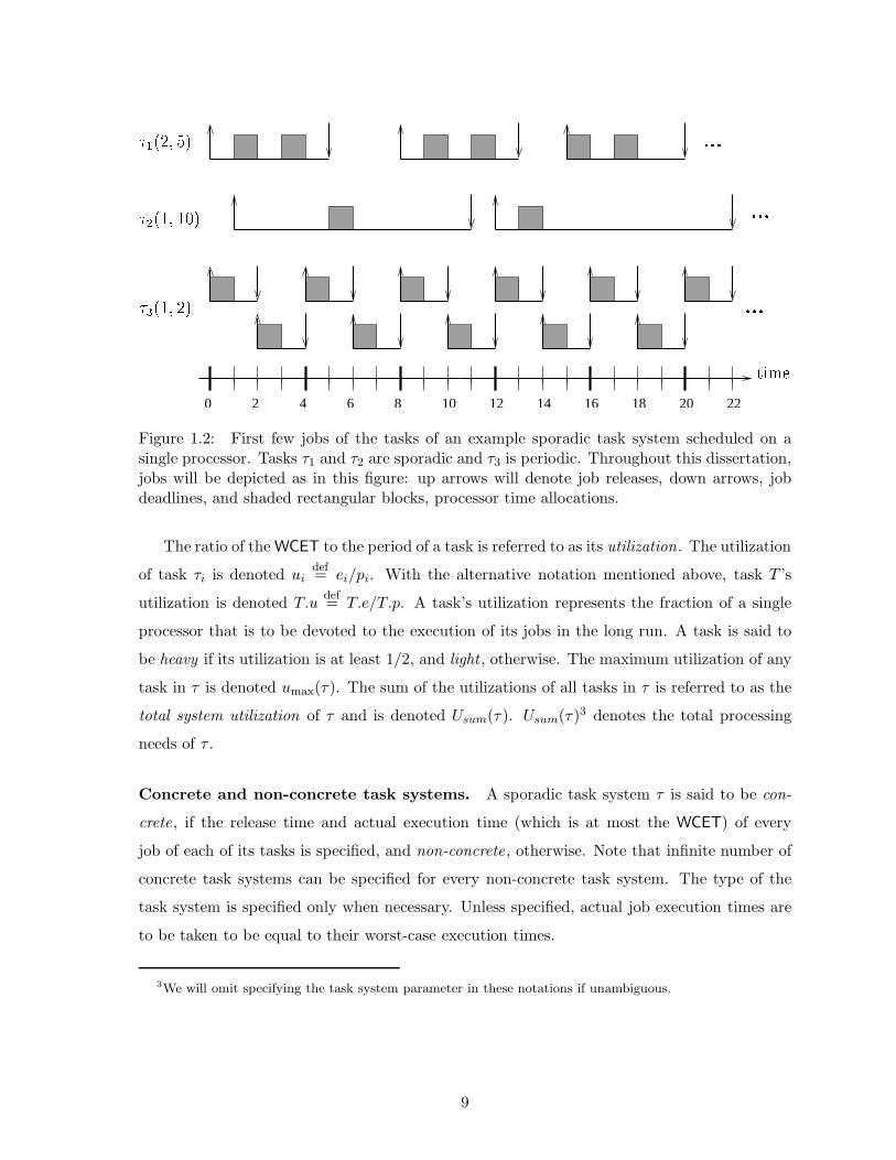
1.2 Illustration of pictorial depiction used with sporadic tasks . . . . . . . . . . . . 9

1.3 Architecture of an SMP . . . . . . . . . . . . . . . . . . . . . . . . . . . . . . . 10

1.4 Comparison of uniprocessor schedules under EDF, RM, and LLF for an exampletask system . . . . . . . . . . . . . . . . . . . . . . . . . . . . . . . . . . . . . . 15

1.5 Schematic representations of partitioned, global, and two-level hybrid schedulingalgorithms . . . . . . . . . . . . . . . . . . . . . . . . . . . . . . . . . . . . . . . 20

1.6 Sample schedules to compare and contrast partitioning and full-migration algo-rithms . . . . . . . . . . . . . . . . . . . . . . . . . . . . . . . . . . . . . . . . . 24

1.7 Sample schedules to compare and contrast partitioning and restricted-migrationalgorithms . . . . . . . . . . . . . . . . . . . . . . . . . . . . . . . . . . . . . . . 26

2.1 Schedules for two concrete instances of a skippable task system . . . . . . . . . 43

2.2 Sample value functions . . . . . . . . . . . . . . . . . . . . . . . . . . . . . . . . 54

3.1 A g-EDF schedule with a deadline miss for a feasible task system . . . . . . . . 57

3.2 An LLF schedule with a deadline miss for a feasible task system . . . . . . . . . 58

3.3 Derivation of pseudo-release times and pseudo-deadlines for subtasks under Pfairscheduling . . . . . . . . . . . . . . . . . . . . . . . . . . . . . . . . . . . . . . . 62

3.4 PF- and IS-windows of subtasks of periodic, sporadic, IS, and GIS tasks . . . . 64

3.5 Group deadlines of subtasks of periodic and IS tasks . . . . . . . . . . . . . . . 65

3.6 Allocations in an ideal schedule to subtasks of periodic and GIS tasks . . . . . 69

3.7 Sample schedules under PD2, EPDF, and WM . . . . . . . . . . . . . . . . . . . 74

3.8 Hierarchical scheduling using supertasks . . . . . . . . . . . . . . . . . . . . . . 77

3.9 Time-based task classification, and displacement of subtasks triggered by theremoval of other subtasks . . . . . . . . . . . . . . . . . . . . . . . . . . . . . . 80

4.1 Sample task systems with unbounded tardiness under partitioned EDF andglobal RM . . . . . . . . . . . . . . . . . . . . . . . . . . . . . . . . . . . . . . . 84

4.2 Deadline misses under g-EDF due to early releasing . . . . . . . . . . . . . . . . 87

xiv

4.3 Tardiness bounds under g-EDF and g-NP-EDF as functions of average task uti-lization . . . . . . . . . . . . . . . . . . . . . . . . . . . . . . . . . . . . . . . . 113

4.4 Tardiness bounds under g-EDF and g-NP-EDF as functions of number of processors114

4.5 Sample g-EDF schedule with tardiness emax − 1 on two processors . . . . . . . . 116

4.6 Sample g-EDF schedules for extended sporadic task systems . . . . . . . . . . . 118

4.7 Application of the extended task model to tasks with variable per-job executioncosts . . . . . . . . . . . . . . . . . . . . . . . . . . . . . . . . . . . . . . . . . . 119

4.8 Empirical comparison of the three tardiness bounds derived for g-EDF and g-

NP-EDF by varying task execution costs . . . . . . . . . . . . . . . . . . . . . . 122

4.9 Empirical comparison of the three tardiness bounds derived for g-EDF and g-

NP-EDF by varying task utilizations . . . . . . . . . . . . . . . . . . . . . . . . 123

4.10 Empirical comparison of tardiness bounds derived for g-EDF and g-NP-EDF totardiness observed in practice . . . . . . . . . . . . . . . . . . . . . . . . . . . . 124

5.1 Algorithm Assign-Tasks . . . . . . . . . . . . . . . . . . . . . . . . . . . . . . 129

5.2 Example task assignment . . . . . . . . . . . . . . . . . . . . . . . . . . . . . . 130

5.3 Illustration of processor linkage . . . . . . . . . . . . . . . . . . . . . . . . . . . 132

5.4 Schematic representation of EDF-fm in the execution phase . . . . . . . . . . . 133

5.5 Distributing periodically released jobs of a migrating task between its processors 134

5.6 Complementary Pfair schedule . . . . . . . . . . . . . . . . . . . . . . . . . . . 136

5.7 Relating distribution of jobs of a migrating task between its processors to acomplementary Pfair schedule . . . . . . . . . . . . . . . . . . . . . . . . . . . . 139

5.8 Empirical comparison of tardiness bounds for EDF-fm under different task as-signment heuristics on four processors by varying task execution cost . . . . . . 156

5.9 Empirical comparison of tardiness bounds for EDF-fm under different task as-signment heuristics on eight processors by varying task execution cost . . . . . 157

5.10 Empirical comparison of tardiness bounds for EDF-fm under different task as-signment heuristics on four and eight processors by varying task utilization . . 158

5.11 Empirical evaluation of successful assignment of heavy tasks under the LUF

heuristic and comparison of estimated and observed tardiness under the LEF

heuristic for EDF-fm . . . . . . . . . . . . . . . . . . . . . . . . . . . . . . . . . 159

5.12 Empirical comparison of tardiness estimated by exponential-time and linear-time formulas to observed tardiness for EDF-fm . . . . . . . . . . . . . . . . . . 161

6.1 Illustration for Lemma 6.13 . . . . . . . . . . . . . . . . . . . . . . . . . . . . . 174

6.2 Illustration for Lemma 6.17 . . . . . . . . . . . . . . . . . . . . . . . . . . . . . 177

xv

6.3 Schedulable utilization bound by Wmax for EPDF, partitioned EDF, and globalfp-EDF . . . . . . . . . . . . . . . . . . . . . . . . . . . . . . . . . . . . . . . . . 185

6.4 Deadline miss under EPDF . . . . . . . . . . . . . . . . . . . . . . . . . . . . . . 187

7.1 Counterexample to prove that tardiness under EPDF can exceed one quantum . 191

7.2 Miss Initiator (MI) and Successor of Miss Initiator (SMI) subtasks in EPDF

schedules . . . . . . . . . . . . . . . . . . . . . . . . . . . . . . . . . . . . . . . 197

8.1 Windows of jobs of a periodic task with non-integral period . . . . . . . . . . . 238

8.2 Windows of subtasks of a periodic task with non-integral period . . . . . . . . 239

9.1 Accounting for tick-scheduling overhead in a non-Pfair algorithm . . . . . . . . 253

9.2 Example g-NP-EDF schedules with zero and non-zero overhead . . . . . . . . . 259

9.3 Example g-EDF schedules with zero and non-zero overhead . . . . . . . . . . . 260

9.4 Example to illustrate that if a job of task U resumes after a job of task Tcompletes, then U.D > T.D need not hold . . . . . . . . . . . . . . . . . . . . . 261

9.5 Example g-EDF schedule to illustrate some complexities in ensuring that a jobwhose execution spans contiguous quanta is not migrated needlessly . . . . . . 263

9.6 Schedulability results for M = 2, Q = 1000µs, pmin = 10ms, pmax = 100ms,WSS = 4K . . . . . . . . . . . . . . . . . . . . . . . . . . . . . . . . . . . . . . 281

9.7 Tardiness bounds results for M = 2, Q = 1000µs, pmin = 10ms, pmax = 100ms,WSS = 4K . . . . . . . . . . . . . . . . . . . . . . . . . . . . . . . . . . . . . . 282



9.10 Schedulability results for M = 2, Q = 1000µs, pmin = 10ms, pmax = 100ms,WSS = 128K . . . . . . . . . . . . . . . . . . . . . . . . . . . . . . . . . . . . . 285

9.11 Tardiness bounds results for M = 2, Q = 1000µs, pmin = 10ms, pmax = 100ms,WSS = 128K . . . . . . . . . . . . . . . . . . . . . . . . . . . . . . . . . . . . . 286




xvi




9.18 Schedulability results for bimodal task utilization distribution for M = 2, Q =1000µs, pmin = 10ms, pmax = 100ms, and WSSs of 4K, 64K, and 128K . . . . . 293













9.31 Schedulability results for bimodal task utilization distribution for M = 4, Q =1000µs, pmin = 10, pmax = 100, and WSSs of 4K, 64K, and 128K . . . . . . . . 309


xvii









9.41 Tardiness bounds for M = 8, Q = 1000µs, pmin = 100ms, pmax = 500ms, WSS= 64K . . . . . . . . . . . . . . . . . . . . . . . . . . . . . . . . . . . . . . . . . 319



9.44 Schedulability results for bimodal task utilization distribution for M = 8, Q =1000µs, pmin = 10, pmax = 100, and WSSs of 4K, 64K, and 128K . . . . . . . . 322







xviii

A.1 Job displacements under g-EDF triggered by the removal of other jobs . . . . . 340A.2 An algorithm for choosing tasks for Γ(k1,k2) and Π(k1,k2) when (4.1) does not hold.348

xix

List of Abbreviations

BF Boundary Fair

BWP Blue When Possible

CBS Constant Bandwidth Server

DBP Distance Based Priority

DSP Digital Signal Processing

DTMC Discrete Time Markov Chain

EDF Earliest Deadline First

EDF-fm EDF with Fixed and Migrating tasks

EDF-P-NP EDF with Preemptive and Non-Preemptive segments

EPDF Earliest Pseudo-Deadline First

ER Early Release

FIFO First In First Out

g-EDF global, preemptive EDF

g-NP-EDF global, non-preemptive EDF

GIS Generalized Intra-Sporadic

HUF Highest Utilization First

IS Intra-Sporadic

ISR Interrupt Service Routine

LEF Lowest Execution (cost) First

LITMUSRT LInux Testbed for MUltiprocessor Scheduling in Real-Time Systems

LLF Least Laxity First

LUF Lowest Utilization First

MI Miss Initiator

PD Pseudo-Deadline

pdf probability density function

p-EDF partitioned EDF

PF PFair

PS Processor Sharing (schedule)

QoS Quality-of-Service

r-EDF restricted-migration EDF

xx

RM Rate Monotonic

RRM Rational Rate Monotonic

RTO Red Tasks Only

SMI Successor of Miss Initiator

SMP Symmetric (Shared-Memory) Multiprocessor

SRMS Statistical Rate-Monotonic Scheduling

VR Virtual Reality

WCET Worst-Case Execution Time

WM Weight Monotonic

xxi

Chapter 1

Introduction

The goal of this dissertation is to extend the theory of real-time scheduling to facilitate resource-

efficient implementations of soft real-time systems on multiprocessors. This work is necessi-

tated by the proliferation of both multiprocessor platforms and applications with workloads

that warrant more than one processor and for which soft real-time guarantees are sufficient.

This chapter begins with an introduction to real-time systems followed by a discussion of the

subject matter of this dissertation. Needed background on real-time concepts, including real-

time scheduling on multiprocessors, is then provided. Soft real-time systems are described

next, following which motivation is provided for further research to support such systems on

multiprocessors, and the thesis of this dissertation is stated. The chapter concludes by sum-

marizing the contributions that this dissertation makes in support of the thesis and providing

a roadmap for the rest of the dissertation.

1.1 What is a Real-Time System?

The distinguishing characteristic of a real-time system in comparison to a non-real-time system

is the inclusion of timing requirements in its specification. That is, the correctness of a real-time

system depends not only on logically correct segments of code that produce logically correct

results, but also on executing the code segments and producing correct results within specific

time frames. Thus, a real-time system is often said to possess dual notions of correctness, logical

and temporal . Process control systems, which multiplex several control-law computations,

radar signal-processing and tracking systems, and air traffic control systems are some examples

of real-time systems.

Timing requirements and constraints in real-time systems are commonly specified as dead-

lines within which activities should complete execution. Consider a radar tracking system as

an example. To track targets of interest, the radar system performs the following high-level

activities or tasks: sends radio pulses towards the targets, receives and processes the echo

signals returned to determine the position and velocity of the objects or sources that reflected

the pulses, and finally, associates the sources with targets and updates their trajectories. For

effective tracking, each of the above tasks should be invoked repeatedly at a frequency that

depends on the distance, velocity, and the importance of the targets, and each invocation

should complete execution within a specified time or deadline.

Another characteristic of a real-time system is that it should be predictable. Predictability

means that it should be possible to show, demonstrate, or prove that requirements are always

met subject to any assumptions made, such as on workloads [112]. In this dissertation, we focus

on a priori ensuring that timing requirements are met; ensuring that non-timing requirements

are met is out of the purview of this research.

Hard and soft real-time. Based on the cost of failure associated with not meeting them,

timing constraints in real-time systems can be classified broadly as either hard or soft . A

hard real-time constraint is one whose violation can lead to disastrous consequences such as

loss of life or a significant loss to property. Industrial process-control systems and robots,

controllers for automotive systems, and air-traffic controllers are some examples of systems

with hard real-time constraints. In contrast, a soft real-time constraint is less critical; hence,

soft real-time constraints can be violated. However, such violations are not desirable, either,

as they may lead to degraded quality of service, and it is often the case that the extent of

violation be bounded. Multimedia systems and virtual-reality systems are some examples of

systems with soft real-time constraints.

Three important aspects or components in real-time system design are: real-time system

models including task models and resource models; scheduling algorithms, which determine

how the hardware resources are shared among the system’s threads and/or processes; and

validation tests that determine whether a real-time system’s timing constraints will be met

by a specified scheduling algorithm. Before considering these aspects in detail, we provide

a high-level overview of the research addressed in this dissertation. The ensuing overview is

intended to help place the background material covered later in proper perspective.

2

1.2 Dissertation Focus

As mentioned in the beginning of this chapter, the focus of this dissertation is to improve cost

effectiveness while instantiating soft real-time systems on multiprocessors. The need for work

in this direction is described below.

1.2.1 Motivation

One evident trend in the design of both general-purpose and embedded computing systems

is the increase in the use of multiple processing elements that are tightly coupled. In the

general-purpose arena, this is evidenced by the availability of affordable symmetric multipro-

cessor platforms (SMPs), and the emergence of multicore architectures. In the special-purpose

and embedded arena, examples of multiprocessor designs include network processors, which

are used for packet-processing tasks in programmable routers, system-on-chip platforms for

multimedia processing in set-top boxes and digital TVs, and automotive power-train systems.

If the current shift towards multicore architectures by prominent chip manufacturers such as

Intel [2] and AMD [1] is any indication, then in the future, the standard computing platform

in many settings can be expected to be a multiprocessor, and multiprocessor-based software

designs will be inevitable. The need for multiprocessors is due to both architectural issues

that impose limits on the performance that a single processing unit can deliver, and the preva-

lence of, and ever-increasing need for, higher computing demand from applications. Further,

ideally, the energy consumed by an M -processor system is lower than that consumed by a

single-processor system of equivalent capacity by a factor of approximately M2 [8].

Some embedded systems, such as set-top boxes and automotive systems, are inherently

real-time. Also, a number of emerging real-time applications exist that are instantiated on

general-purpose systems and have high workloads. Systems that track people and machines,

virtual-reality and computer-vision systems, systems that host web-sites, and some signal-

processing systems are a few examples. Timing constraints in several of these embedded- and

general-purpose-system applications are predominantly soft. Hence, with the shift towards

multiprocessors, the need arises to instantiate soft real-time applications on multiprocessors.

1.2.2 Research Need and Overview

Minimizing hardware resource requirements is essential for realizing cost-effective system im-

plementations. One way of minimizing resource requirements is through the careful manage-

3

ment and allocation, i.e., scheduling , of resources to competing requests. Relevant prior work

on uniprocessor and multiprocessor-based soft real-time systems is discussed in Chapter 2. As

can be seen from the discussion there, research on soft real-time scheduling on multiprocessors

has been extremely limited: most prior research on real-time scheduling on multiprocessors

has been confined to hard real-time systems, while that on soft real-time scheduling has been

confined to uniprocessors. Uniprocessor scheduling theory does not readily generalize to mul-

tiprocessors, and basing soft real-time multiprocessor system designs on theory developed for

hard real-time multiprocessor systems can be wasteful. Below, we give an example-driven

explanation for why the latter holds and a high-level overview of some of the issues addressed

in this dissertation. Later, in Section 1.6, a more technical explanation is provided after some

needed background and concepts are set in place.

Example 1.1. Consider a real-time system composed of three sequential processes or

tasks,1 to be instantiated on two identical processors. Starting at time 0, each task periodically

submits four units of work, also referred to as a job1, once every six time units. (In other words,

each task has a period of six time units and each job has an execution requirement of four time

units.) Let the deadline of job k of each task, where k ≥ 1, be at time 6k. That is, each job is

to complete execution before the next job of the same task arrives. Three possible algorithms

for scheduling the tasks in this example are considered below.

Algorithm 1: In the first algorithm that we consider, one of the tasks, say Task 1, is assigned

to Processor 1, and the remaining tasks to Processor 2. That is, the tasks are partitioned

between the two processors, and each task runs exclusively on the processor to which it is

assigned. On each processor, a pending job with the earliest deadline is executed at every

instant, with ties resolved arbitrarily. A schedule for the task system based on this algorithm

is shown in Figure 1.1(a). Under this algorithm, tasks do not migrate between processors, but

as can be seen, Processor 2 is overloaded and jobs assigned to it miss deadlines. The amount

of time by which a deadline is missed, referred to as tardiness, increases with time. In this

example, the kth job of the third task misses its deadline by 2k time units, for all k, and that

of the second task by 2(k − 2) time units, for k ≥ 2. Thus, tardiness for the jobs assigned on

Processor 2 grows without bound.

1Refer to Section 1.3.1 for formal definitions.

4

� � � � � ��

� � � � � ��

� � � � � ��

��

�

��

�

��

��

��

��

��

��

��

��

�

��

��

� �

��

��

��

��

��

��

��

��

��

� ��

� ��

��

��

��

��

��

��

��

��

��

��

��

�� !�� "� !� � �"� !� � �� !��

# $ %��# $ ��&��

' ( ) ( * +

��,

��,

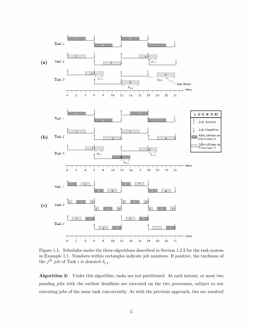
Figure 1.1: Schedules under the three algorithms described in Section 1.2.2 for the task systemin Example 1.1. Numbers within rectangles indicate job numbers. If positive, the tardiness ofthe jth job of Task i is denoted δi,j.

Algorithm 2: Under this algorithm, tasks are not partitioned. At each instant, at most two

pending jobs with the earliest deadlines are executed on the two processors, subject to not

executing jobs of the same task concurrently. As with the previous approach, ties are resolved

5

arbitrarily. A schedule based on this algorithm is shown in Figure 1.1(b). In this schedule,

the third task migrates between the two processors, and its jobs suffer from a tardiness of two

time units.

Algorithm 3. Finally, we consider scheduling using a more elaborate set of rules (the

specifics of which are not of interest for the moment) that can ensure that no deadlines will

be missed. A schedule under this set of rules is shown in Figure 1.1(c). Though no deadline is

missed in this schedule, note that not only do tasks migrate, but every job migrates at least

once. (Each job of the second task migrates twice.)

For the task system under consideration, it is easily seen that at least three processors

are required to ensure that no deadlines will be missed under the first two algorithms. From

Figure 1.1(b), it appears that under the second algorithm, no deadline will be missed by more

than two time units. If this is the case and if bounded tardiness is tolerable, then, even though

tasks may migrate under it, the second algorithm may be used to instantiate the system on

just two processors, and thereby, lower the number of processors by one-third. However, real-

time scheduling theory as it exists today has no tools for reliably predicting the tardiness to

which arbitrary task systems may be subject under various scheduling algorithms, and in turn,

lowering resource requirements, when bounded tardiness is tolerable. One of the goals of this

dissertation is to extend the theory in such a direction.

Though no deadline is missed under the third algorithm, it has its own limitations, which

are described in detail later in Section 1.6. One limitation is the increased number of preemp-

tions and/or migrations for jobs, which can lead to poor cache usage, and hence, degraded

performance, in practice. Furthermore, the somewhat complex scheduling model and the re-

strictions that the algorithm imposes can also take useful processor time away from the tasks

and may in fact be overkill for soft real-time systems. For instance, one restriction of the

algorithm is that job execution costs and periods be integer multiples of the quantum size,

necessitating non-integral execution costs to be rounded up to the next integral value. For

example, an execution cost of, say, 4.1 quanta would have to be rounded up to 5.0 quanta,

which means that every fifth quantum allocated to the corresponding task would have to be

partially wasted. A second goal of this dissertation is to propose techniques for scheduling

when not all such restrictions can be satisfied and to determine the loss to timeliness that

relaxing the restrictions entails.

With the above overview of the research addressed in this dissertation, we turn to providing

6

needed background on real-time systems and scheduling. We begin with a description of the

real-time system model assumed in this dissertation.

1.3 Real-Time System Model

To ensure that a real-time system is predictable, a priori knowledge of the workload of the

system and available resources is necessary. A real-time task model is used to describe the

workload and timing requirements of a real-time application, and a resource model is used to

describe the resources that are available for instantiating the application. In this section, we

first describe a commonly used hard real-time task model, upon which the soft real-time task

model considered in this dissertation is based. The resource model that we assume is described

afterward.

1.3.1 Hard Real-Time Task Model

In real-time terminology, a chunk of sequential work that is associated with a timing constraint

(deadline) and submitted to the scheduler is referred to as a job. Thus, a simple model of a

real-time system is a set of jobs, each of which is associated with an arrival or release time,

a deadline, and a worst-case execution time (WCET). The release time of a job is the time

before which the job cannot commence execution and its WCET is the maximum time that

the job will execute on a dedicated processor. (If more than one processor, not all of which

are identical, are part of the system’s resource pool, then it is assumed that the WCET of each

job is specified or can be determined for each processor.) However, enumerating all jobs is

generally infeasible for most but short-lived systems, necessitating more concise models.

Periodic and sporadic tasks. As in the radar tracking system described in Section 1.1,

many real-time systems consist of one or more sequential segments of code, each of which is

invoked repeatedly and each of whose executions should complete within a specified amount

of time. Each recurring segment of code is generally designed and implemented as a separate

thread or process, and, in the terminology of real-time systems, is referred to as a task . Tasks

can be invoked in response to events in the external environment that the system interacts

with, events in other tasks, or the passage of time implemented using timers. Each invocation

of a task constitutes a job, and unless otherwise specified, a task is long-lived, and can be

invoked an infinite number of times, i.e., can generate jobs indefinitely. Hence, many real time

7

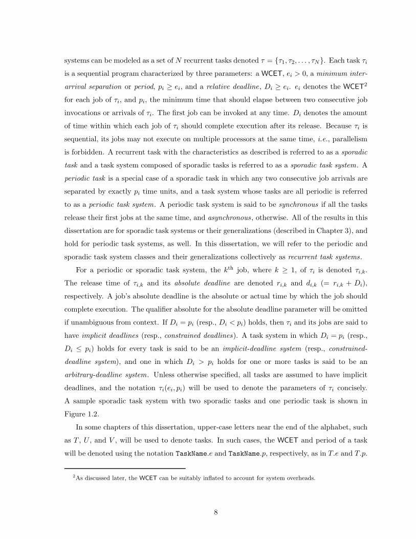
systems can be modeled as a set of N recurrent tasks denoted τ = {τ1, τ2, . . . , τN}. Each task τi

is a sequential program characterized by three parameters: a WCET, ei > 0, a minimum inter-

arrival separation or period, pi ≥ ei, and a relative deadline, Di ≥ ei. ei denotes the WCET2

for each job of τi, and pi, the minimum time that should elapse between two consecutive job

invocations or arrivals of τi. The first job can be invoked at any time. Di denotes the amount

of time within which each job of τi should complete execution after its release. Because τi is

sequential, its jobs may not execute on multiple processors at the same time, i.e., parallelism

is forbidden. A recurrent task with the characteristics as described is referred to as a sporadic

task and a task system composed of sporadic tasks is referred to as a sporadic task system. A

periodic task is a special case of a sporadic task in which any two consecutive job arrivals are

separated by exactly pi time units, and a task system whose tasks are all periodic is referred

to as a periodic task system. A periodic task system is said to be synchronous if all the tasks

release their first jobs at the same time, and asynchronous, otherwise. All of the results in this

dissertation are for sporadic task systems or their generalizations (described in Chapter 3), and

hold for periodic task systems, as well. In this dissertation, we will refer to the periodic and

sporadic task system classes and their generalizations collectively as recurrent task systems.

For a periodic or sporadic task system, the kth job, where k ≥ 1, of τi is denoted τi,k.

The release time of τi,k and its absolute deadline are denoted ri,k and di,k (= ri,k + Di),

respectively. A job’s absolute deadline is the absolute or actual time by which the job should

complete execution. The qualifier absolute for the absolute deadline parameter will be omitted

if unambiguous from context. If Di = pi (resp., Di < pi) holds, then τi and its jobs are said to

have implicit deadlines (resp., constrained deadlines). A task system in which Di = pi (resp.,

Di ≤ pi) holds for every task is said to be an implicit-deadline system (resp., constrained-

deadline system), and one in which Di > pi holds for one or more tasks is said to be an

arbitrary-deadline system. Unless otherwise specified, all tasks are assumed to have implicit

deadlines, and the notation τi(ei, pi) will be used to denote the parameters of τi concisely.

A sample sporadic task system with two sporadic tasks and one periodic task is shown in

Figure 1.2.

In some chapters of this dissertation, upper-case letters near the end of the alphabet, such

as T , U , and V , will be used to denote tasks. In such cases, the WCET and period of a task

will be denoted using the notation TaskName.e and TaskName.p, respectively, as in T.e and T.p.

2As discussed later, the WCET can be suitably inflated to account for system overheads.

8

0 2 4 6 8 10 12 14 16 18 20 22

-./0

12345 67

18 395 9:7

1; 395 47

<<<

<<<

<<<

Figure 1.2: First few jobs of the tasks of an example sporadic task system scheduled on asingle processor. Tasks τ1 and τ2 are sporadic and τ3 is periodic. Throughout this dissertation,jobs will be depicted as in this figure: up arrows will denote job releases, down arrows, jobdeadlines, and shaded rectangular blocks, processor time allocations.

The ratio of the WCET to the period of a task is referred to as its utilization. The utilization

of task τi is denoted uidef= ei/pi. With the alternative notation mentioned above, task T ’s

utilization is denoted T.udef= T.e/T.p. A task’s utilization represents the fraction of a single

processor that is to be devoted to the execution of its jobs in the long run. A task is said to

be heavy if its utilization is at least 1/2, and light , otherwise. The maximum utilization of any

task in τ is denoted umax(τ). The sum of the utilizations of all tasks in τ is referred to as the

total system utilization of τ and is denoted Usum(τ). Usum(τ)3 denotes the total processing

needs of τ .

Concrete and non-concrete task systems. A sporadic task system τ is said to be con-

crete, if the release time and actual execution time (which is at most the WCET) of every

job of each of its tasks is specified, and non-concrete, otherwise. Note that infinite number of

concrete task systems can be specified for every non-concrete task system. The type of the

task system is specified only when necessary. Unless specified, actual job execution times are

to be taken to be equal to their worst-case execution times.

3We will omit specifying the task system parameter in these notations if unambiguous.

9

Multi−

level

Cache

Multi−

level

Cache

Multi−

level

Cache

. . . .Processor Processor Processor

Processor−Memory Interconnect (e.g. bus)

Memory

. . .

Figure 1.3: Architecture of a symmetric shared-memory multiprocessor (SMP). The processorsare replicas of one another, are provided with identical caches, and have uniform access to acentralized main memory.

1.3.2 Resource Model

The focus of this dissertation is designing and analyzing algorithms for efficiently scheduling

soft real-time task systems on the processors of an identical multiprocessor platform. Through-

out this dissertation, M ≥ 2 will denote the number of processors. As its name suggests, the

processors of an identical multiprocessor are replicas of one another and have the same char-

acteristics, including uniform access times (in the absence of contention) to memory. Uniform

memory access is accomplished by the use of a centralized memory that is shared among pro-

cessors. This type of multiprocessor is commonly referred to as a symmetric shared-memory

multiprocessor (SMP). Refer to Figure 1.3 for an illustration. Each processor may be provided

with one or more levels of identical caches (instruction, data, and unified) to expedite access

to frequently accessed addresses and/or addresses that are spatially close. It is assumed that

every task is equally capable of executing on every processor and that there is no restriction

on the processors that a task may execute upon. However, the presence of caches suggests

that the execution time of a job is likely to be more if the job executes on multiple proces-

sors (different processors at different times), i.e., if the job migrates, than if it executes on a

10

single processor. To lower migration overheads, a scheduling algorithm may choose to restrict

executing a task or a job to one or a subset of the processors, even though the system model

imposes no restriction. Overheads due to migration are discussed in detail in a later section.

Accounting for migration and system overheads while designing a real-time system is discussed

below in Section 1.3.3.

Tasks in many real-time systems require access to resources other than processors, such

as memory, I/O, and network bandwidth. Similarly, tasks in many real-time systems are

not completely independent. A task system is said to be independent if the execution of

none of its tasks depends on the status of one or more of the other tasks. Some factors

contributing to interdependence among tasks are synchronization constraints imposed by pro-

ducer/consumer relationships [69] and a need to access to shared data structures, I/O devices,

etc., in a mutually-exclusive manner, and precedence constraints, which restrict the order in

which tasks may execute. In the presence of such interdependencies, tasks may block or be sus-

pended, which will add new considerations in reasoning about resource-allocation algorithms.

Integrated and holistic techniques for synergistically allocating multiple types of resources that

are cognizant of synchronization and precedence constraints, and reasoning about such tech-

niques, begin with and make use of scheduling and analytic techniques for resources of a single

type. This dissertation is concerned with efficiently allocating multiple copies of the processor

resource (i.e., identical processors) to a soft real-time system. Allocating multiple resource

types and dealing with synchronization and precedence constraints are beyond the scope of

this dissertation.

1.3.3 Accounting for Overheads

Task preemptions and context switches, task migrations, and the act of scheduling itself are

infrastructure or system overheads that are extrinsic to and take time away from the application

tasks at hand. Hence, any validation approach that does not account for time lost due to

overheads cannot be guaranteed to be correct. Note that no provisions are included in the

task model per se for overheads. In a well-known method for accounting for overheads, each

extrinsic activity (e.g., a preemption, migration, or scheduler invocation) is charged to a unique

job, and the WCET of each task is inflated by the maximum cumulative time required for all

the extrinsic activities charged to any of its jobs. The extent of the overhead due to each

source can vary with the scheduling algorithm, and hence, an algorithm with good properties

when overheads are ignored can perform poorly in practice. Therefore, any comparison of

11

algorithms that ignores the overheads is deficient from a practical standpoint. Throughout this

dissertation, we will assume that system overheads are included in the WCETs of tasks using

efficient charging methods. The WCET of a task is therefore dependent on the implementation

platform, application characteristics, and the scheduling algorithm.4

1.4 Real-Time Scheduling Algorithms and Validation Tests

A scheduling algorithm allocates processor time to tasks, i.e., determines the execution-time

intervals and processors for each job while taking any restrictions, such as on concurrency,

into account. In real-time systems, processor-allocation strategies are driven by the need to

meet timing constraints. Before getting into a discussion of possible scheduling approaches,

we define some terms and metrics commonly used in describing some properties of real-time

scheduling algorithms and in comparing different algorithms.

1.4.1 Definitions

Feasibility, schedulability, and optimality. A task system τ is said to be feasible on a

hardware platform if there is some way of scheduling and meeting all the deadlines of τ on that

platform. τ is said to be schedulable on a hardware platform by algorithm A, if A is capable

of correctly scheduling τ on that platform, i.e., can meet all the deadlines of τ . A is said to

be an optimal scheduling algorithm if A can correctly schedule every feasible task system for

every hardware platform. It is often useful to restrict the definition of optimality to a subset of

task systems (such as periodic or sporadic task systems) or to a class of scheduling algorithms

or both. When restricted to task system subsets, A is said to be optimal for a subset S of

task systems, if A can correctly schedule every feasible task system of subset S, and when

restricted to algorithm classes,5 A is said to be an optimal class-C scheduling algorithm, if A

can correctly schedule every task system that can be correctly scheduled by some algorithm in

class C. Optimality can similarly be restricted to hardware platform classes, with uniprocessors

and multiprocessors being the most-commonly considered classes.

4Alternatively, the task model can be altered to specify the WCET of a task in the absence of interferences,and explicitly list the sources of interferences and their worst-case costs. We have followed the approach thatis customary in the real-time literature.

5Algorithm classification is discussed in Section 1.4.2.

12

Schedulable utilization bound. A useful and common metric for comparing different

scheduling algorithms with respect to their effectiveness in meeting the deadlines of a recur-

rent task system is the schedulable utilization bound . Formally, if UA(M,α) is a schedulable

utilization bound, or more concisely, utilization bound , for scheduling algorithm A, then on

M processors, A can correctly schedule every recurrent task system τ with umax(τ) ≤ α and

Usum(τ) ≤ UA(M,α). If, in addition, there exists at least one task system with total utilization

UA(M,α) and umax = α, whose task parameters can be slightly modified such that Usum and

umax are higher than UA(M,α) and α, respectively, by infinitesimal amounts, and the modified

task system has a deadline miss under A on M processors, then UA(M,α) is said to be the min-

imax utilization6 of A for M and umax; otherwise, UA(M,α) is a lower bound on A’s minimax

utilization for M and umax. The minimax utilization of A is also referred to as the worst-case

schedulable utilization7 of A. Furthermore, if no task system with total utilization exceeding

UA(M,α) can be scheduled correctly by A when umax = α on M processors, then UA(M,α)

is said to be the optimal utilization bound of A for M and umax. Note that while an optimal

utilization bound is also a worst-case schedulable utilization, the converse may not hold. This

is because, it is possible that there exist task systems that are correctly scheduled but have a

total utilization that is higher than that of some task system that is barely schedulable (i.e.,

some worst-case schedulable utilization). It should also be noted that when expressed using a

fixed set of parameters, such as α and M , different values are not possible for the optimal and

worst-case schedulable utilizations. In other words, if an optimal utilization bound exists for

M and α, then a worst-case schedulable utilization that is different from the optimal bound

is not possible.

Schedulability tests. In addition to serving as a comparison metric, schedulable utilizations

of scheduling algorithms can also be used in devising simple and fast validation tests and online

admission-control tests for the algorithms. In the context of hard real-time systems, validation

tests are generally referred to as schedulability tests. Given the schedulable utilization UA(M)

of Algorithm A and a task system τ , an O(N)-time schedulability test for τ under A that

6The phrase minimax utilization is due to Oh and Baker [93] and denotes the minimum utilization over allmaximal task sets. A maximal task set is one that is schedulable but if the execution times of its tasks areincreased slightly, then some deadline will be missed.

7Unless otherwise specified, worst-case schedulable utilizations are assumed to be with respect to M andα = umax. It is possible to obtain other worst-case values if other or more task parameters, such as executioncosts and periods, are considered.

13

verifies whether Usum(τ) is at most UA(M), and a similar O(1) per-task time online admission

control test, are straightforward. The downside of such utilization-based schedulability tests

is that for many algorithms, optimal schedulable utilizations are not known. In such cases,

the tests are only sufficient but not necessary (i.e., are not exact tests), and hence, can be

pessimistic, i.e., incorrectly conclude that deadlines may be missed.

1.4.2 Real-Time Scheduling Strategies and Classification

In general, since job release times are not known a priori , pre-computing schedules off-line is

not possible with sporadic and some asynchronous periodic task systems. As a result, online

scheduling algorithms are needed. Typically, such an algorithm assigns a priority to each job,

and on an M -processor system, schedules for execution the M jobs with the highest priorities

at any instant, subject to not violating constraints on migrations,8 preemptions, concurrency,

and mutually-exclusive executions, if any. We will consider scheduling9 on uniprocessors first

and that on multiprocessors afterwards.

1.4.2.1 Scheduling on Uniprocessors

In real-time systems, the need to meet timing requirements suggests using strategies optimized

for that purpose. Giving higher priority to (i) jobs with earlier deadlines, (ii) those with

smaller slack times,10 or (iii) jobs of tasks that recur at a higher rate (i.e., tasks with shorter

periods) are some logically reasonable strategies for selecting jobs to execute in real-time

systems. All of these are greedy strategies because each makes a choice that appears to be the

best at the moment.

The algorithm that uses the first strategy is called earliest-deadline-first (EDF) [46]. EDF’s

greedy strategy turns out to be optimal for scheduling sporadic tasks on a uniprocessor [82].

Similarly, least-laxity-first (LLF) [91], also referred to as smallest-slack-first , is a scheduling

algorithm, which directly uses the second strategy, and which is also optimal for sporadic task

systems on a uniprocessor. Lastly, under the well-known and widely-used rate-monotonic (RM)

scheduling algorithm, the third strategy of prioritizing tasks with shorter periods over those

with longer periods is employed. Partial schedules under the three algorithms referred to are

8Refer to Section 1.4.2.2 for a discussion on the degree of task migrations.

9Unless otherwise specified, any reference to scheduling is to online approaches.

10The slack time of a job at any given time is the difference between the amount of time remaining until thejob’s deadline and its pending or unfulfilled execution requirement.

14

time

0 2 4 6 8 10 12 14 16 18 20 22

τ2(4,10)

τ1(3,5)

time

0 2 4 6 8 10 12 14 16 18 20 22

τ2(4,10)

τ1(3,5)

time

0 2 4 6 8 10 12 14 16 18 20 22

τ2(4,10)

τ1(3,5)

. . .

. . .

. . .

. . .

. . .

. . .

(a)

(b)

(c)

Figure 1.4: Uniprocessor schedules under (a) EDF, (b) RM, and (c) LLF for a task systemwith two tasks τ1(3, 5) and τ2(4, 10).

shown in Figure 1.4 for the first few jobs of a task system with two tasks τ1(3, 5) and τ2(4, 10).

The three algorithms differ in the complexity of their priority schemes and their ability to

meet the timing constraints and form the basis of a priority-based classification of scheduling

algorithms presented in [42]. Before describing that classification, we briefly mention two other

15

ways of classifying scheduling algorithms.

Preemptive and non-preemptive algorithms. Under preemptive algorithms, the execu-

tion of a running job can be interrupted any time before its completion and resumed later. In

general, under real-time scheduling algorithms, a job is preempted only if another job with a

higher priority arrives when every processor is busy. Under non-preemptive algorithms, a job

may not be interrupted once it commences execution, and thus is guaranteed uninterrupted

execution until completion. As described, preemptivity is associated with algorithms. Alter-

natively, preemptivity can be associated with tasks and it is often useful to consider hybrid

schemes wherein whether a job can be preempted depends on whether it executes in a pre-

emptive or non-preemptive section. Unless otherwise specified, it is to be assumed that jobs

are fully preemptable.

Work-conserving and non-work-conserving algorithms. An algorithm is said to be

work conserving if it does not idle any processor when one or more jobs are pending, and non-

work conserving , otherwise. The most common reason for inserting idle times is to improve

schedulability. For instance, under non-preemptive algorithms, idling may prevent binding a

job prematurely to a processor, and hence, has the potential to correctly schedule task systems

that are otherwise not schedulable. However, the time complexity associated with deciding

whether idling can improve schedulability can be quite high, and hence, generally (barring a

few exceptions)10 only off-line schedulers tend to be non-work-conserving. All the algorithms

considered in this dissertation, except some Pfair-related algorithms [25], are work conserving.

Priority-Based Classification

Based on how jobs and tasks are prioritized, scheduling algorithms can be classified into the

following three categories.

Static-priority algorithms (Ps). Under a static-priority algorithm, each task is assigned

a priority off-line, which is then assigned to each of its jobs at run-time. Thus, the priority of

a task remains static, i.e., unchanged, across job invocations. The RM scheduling algorithm

10As originally designed, Pfair scheduling algorithms [25], which can optimally schedule recurrent real-timetask systems on multiprocessors, are not work-conserving. However, it has been shown that such a behavioris not necessary to improve schedulability under Pfair scheduling. This issue is discussed in more detail inChapter 3.

16

mentioned above is an example of an algorithm in this class. RM is also an optimal static-

priority scheduling algorithm for sporadic task systems on uniprocessors if relative deadlines

are equal to periods as assumed in this dissertation.

Restricted-dynamic-priority algorithms (P rd ). The algorithms in this class are also re-

ferred to as task-level dynamic-priority and job-level fixed-priority algorithms in the literature.

Generally, under this class of algorithms, the priority of a job is determined at run-time, and

hence, different jobs of a task can be assigned different priorities. However, once assigned, the

priority of a job cannot be changed. EDF is an algorithm in this class.

Unrestricted-dynamic-priority algorithms (P ud ). This third class relaxes the restriction

of the previous class by allowing a given job to be assigned different priorities at different times.

Hence, the relative priorities between two jobs can change with time. LLF, described earlier,

is an example of an algorithm in this class.

Comparison of the Priority Classes

The restricted-dynamic-priority class generalizes the static-priority class and is in turn gener-

alized by the unrestricted-dynamic-priority class. The effectiveness of an algorithm in meeting

timing constraints can be expected to improve with increasing generalization. However, on the

negative side, the implementation complexity, and run-time overheads, such as the number of

context switches due to preemptions, can also increase at the same time. Below, we compare

the three classes on the basis of their overheads and schedulability. Since RM, EDF, and LLF

are optimal scheduling algorithms for their respective classes on uniprocessors [82, 91], we

often take these three algorithms to be representatives for their classes.

Overhead comparison. Though the worst-case time complexity of selecting the highest-

priority job is O(log N) (where N is the number of tasks) for each of RM, EDF, and LLF,

simpler implementations that are fast in practice are possible for RM and other static-priority

algorithms [84]. The maximum possible number of job preemptions, when expressed as a

function of the total number of jobs, is asymptotically comparable for the static and restricted-

dynamic-priority classes. However, in practice, the actual number can be higher for RM than

for EDF [39]. Preemptions can be expected to be much higher for the unrestricted-dynamic-

priority class and will depend on the rate at which job priorities change. For example, in

17

Figure 1.4, the number of preemptions under RM is twice that under EDF, and is the highest

under LLF. In addition to context switches, some cache-related overheads12 are also possible

due to preemptions, and hence, it is desirable that their number be minimized.

Schedulability comparison. On a single processor, the worst-case schedulable utilization

of RM for sporadic task systems is URM = N · (21/N − 1) [82], which is strictly decreasing

with N and converges to ln 2 ≈ 0.69 as N −→ ∞. On the other hand, the schedulable

utilization bound for EDF is 1.0 for all N [82]. Thus, on a uniprocessor, moving from static to

restricted-dynamic-priority algorithms can significantly enhance schedulability in many cases.

Furthermore, because no algorithm can correctly schedule any task system with total system

utilization exceeding 1.0 on a uniprocessor, EDF is optimal not only for its class, but universally,

i.e., for the class encompassing all scheduling algorithms.

It should also be mentioned that the utilization-bound-based schedulability test for RM is

only a sufficient test and can be pessimistic. In [77], Lehoczky et al. devised a more accurate

but complex test for RM, which is necessary and sufficient for sporadic task systems but is only

sufficient for asynchronous, periodic task systems. Using this exact characterization of RM,

Lehoczky et al. also showed that the utilization bound of RM can be taken to be around 88%

on an average. Given that RM is an optimal static-priority scheduling algorithm, there is still

approximately a schedulability loss of 12% under the static-priority class on a uniprocessor.

Because EDF is universally optimal, the additional flexibility in scheduling offered by the

unrestricted-dynamic-priority class (LLF, which belongs to the class, is also universally optimal)

provides no extra benefit at least for independent task systems. Further, since their run-

time overheads tend to be higher, unrestricted-dynamic-priority algorithms are not considered

interesting on uniprocessors.

1.4.2.2 Scheduling on Multiprocessors

In this subsection, we consider multiprocessor scheduling in some detail.

Multiprocessor Scheduling Approaches

Two approaches traditionally considered for scheduling on multiprocessors are partitioning and

global scheduling .

12Cache-related overheads due to preemptions and migrations are discussed further towards the end of Sec-tion 1.4.2.2.

18

Partitioning. Under partitioning, the set of tasks is statically partitioned among processors,

that is, each task is assigned to a unique processor upon which all its jobs execute. Each

processor is associated with a separate instance of a uniprocessor scheduler for scheduling the

tasks assigned to it and a separate local ready queue for storing its ready jobs. In other words,

the priority space associated with each processor is local to it. The different per-processor

schedulers may all be based on the same scheduling algorithm or use different ones. The

algorithm that partitions the tasks among processors should ensure that for each processor,

the sum of the utilizations of tasks assigned to it is at most the utilization bound of its

scheduler. Scheduling under this model is depicted in Figure 1.5(a).

Global scheduling. In contrast to partitioning, under global scheduling, a single, system-

wide, priority space is used, and a global ready queue is used for storing ready jobs. At

any instant, at most M ready jobs with the highest priority (in the global priority space)

execute on the M processors. No restrictions are imposed on where a task may execute; not

only can different jobs of a task execute on different processors, but a given job can execute on

different processors at different times, subject to not violating restrictions on non-preemptivity.

Figure 1.5(b) illustrates global scheduling.

Two-level hybrid scheduling. Some algorithms do not strictly fall under either of the

above two categories, but have elements of both. For example, algorithms for scheduling sys-

tems in which some tasks cannot migrate and have to be bound to a particular processor, while

others can migrate, follow a mixed strategy. In general, scheduling under a mixed strategy is

at two levels: at the first level, a single, global scheduler determines the processor that each

job should be assigned to using global rules, while at the second level, the jobs assigned to

individual processors are scheduled by per-processor schedulers using local priorities. Several

variants of this general model and other types of hybrid scheduling are also possible. Typically,

the global scheduler is associated with a global queue of ready, but unassigned, jobs, and the

per-processor schedulers with queues that are local to them. Elements of one type of hybrid

scheduling are illustrated in Figure 1.5(c).

Migration-Based Classification

As can be seen, the extent to which tasks migrate across processors differs under the three

scheduling approaches discussed above. Hence, apart from a priority-based classification de-

19

Per−Processor

Schedulers

(Second−Level)

Per−Processor

Schedulers

= == => >> >

? ?? ?@ @@ @

Processors

Global

Scheduler

Processors

Scheduler

Task

Partitions

ProcessorsLocal Ready Queues(of ready jobs)

Global Ready Queue

(of ready jobs)

Global

Task Set

Global

Task Set

...

...

...

...

...

...

...

...

Global(First−Level)

Local Ready Queues

. . .

. . .

. . .

. . .

. . .

. . .

(a) (b)

(c)

Global Ready Queue

(of ready jobs)

(of ready jobs unassigned to any processor)

Figure 1.5: Schematic representations of (a) partitioned, (b) global, and (c) two-level hybridscheduling algorithms.

scribed in Section 1.4.2.1, multiprocessor scheduling algorithms can be classified based on the

degree of migration they allow to tasks as well, as suggested by Carpenter et al. in [42]. We

next describe their classification.

20

No-migration or partitioned algorithms (Mp). Under this class of algorithms, task

migration is prohibited. Hence, the algorithms in this class use the partitioning strategy

described above. Partitioned-EDF, in which each per-processor scheduler is EDF, is an example

of an algorithm in this class.

Restricted-migration algorithms (Mr). This class of algorithms allows tasks to migrate

at job boundaries. That is, different jobs of a task can execute on different processors, but a

given job may not migrate and must execute only on a single processor. Some algorithms in

this class may require two-level, hybrid scheduling as described above. Restricted-migration

EDF, referred to as r-EDF and described in [24], is an example of an algorithm in this class that

requires two-level scheduling. Under r-EDF, a global scheduler assigns each newly-arriving job

to a processor that can accommodate it, i.e., can correctly schedule all the jobs previously

assigned to it as well as the new job. The jobs assigned to each processor are scheduled locally

by a second-level EDF scheduler. Second-level scheduling is not required for all the algorithms

in this class and can be eliminated if scheduling rules permit it. Global, non-preemptive EDF

(referred to as g-NP-EDF), with no restrictions on where different jobs execute, is an algorithm

in this class for which single-level scheduling suffices.

Full-migration algorithms (Mf ). A full-migration algorithm places no restriction on inter-

processor migration and uses the global scheduling approach. Global, preemptive EDF (referred

to as g-EDF) is an example of an algorithm in this class.

Carpenter et al. suggested considering each migration class with each priority class, and

hence, nine classes of multiprocessor scheduling algorithms. Their taxonomy of scheduling

algorithms is shown in the form of a matrix in Table 1.1. When convenient, we will denote a

class using a tuple (x, y), where x denotes a priority class (one of Ps, P rd , and P u

d ), and y, a

migration class (one of Mp, Mr, and Mf ). The entries in the table (discussed later) represent

known upper and lower bounds on the worst-case schedulable utilization for each class.

Comparison of Classes of Multiprocessor Schedulers

Schedulability comparison. In [42], Carpenter et al. compare the schedulability of the

classes with respect to two aspects: (i) the set of all task systems that any algorithm in each

class can schedule correctly (which we refer to as raw schedulability) and (ii) the best known

schedulable utilization bounds for any algorithm in each class. Their results are summarized

21

Mf : full M2

3M−2≤ U ≤ M+1

2U = M − α(M − 1), if α ≤ 1

2[61] U = M [25, 105]

migration [16] U = M+12

, otherwise [22]

Mr: U ≤ M+12

U ≥ M − α(M − 1), if α ≤ 12

[24] U ≥ M − α(M − 1), if α ≤ 12

restricted U = M+12

, otherwise [24] U = M+12

, otherwisemigration

Mp: U = M+12

[17] U = βM+1β+1

, where β =⌊

1α

⌋

[86] U = βM+1β+1

, where β =⌊

1α

⌋

partitioned

Ps: static P rd : restricted dynamic P u

d : unrestricted dynamic

Table 1.1: Carpenter et al.’s classification of multiprocessor scheduling algorithms presentedin [42]. Entries in the table represent known lower and upper bounds on the worst-caseschedulable utilization, U , for the different classes of scheduling algorithms. (Some entrieshave been updated to reflect later advances.) α = umax, the maximum utilization of any taskin the task system under consideration. Citations next to the entries indicate their primarysources.

below.

Comparison of raw schedulability. With respect to raw schedulability, Class C1 is said

to be as powerful as (resp., strictly more powerful than) Class C2, if the set of all task systems

correctly scheduled by any algorithm in C2 is a subset of or the same as (resp., proper subset

of) the set of all task systems correctly scheduled by some algorithm in C1. Some salient

raw-schedulability comparisons are as follows.

Comparison within a migration class: Within a migration class, increased generalization

along the priority dimension does not worsen raw schedulability . Specifically, the P rd class

is strictly more powerful than the Ps class when both are subject to the same migration

rules. The two dynamic-priority classes are equally powerful under partitioning and the

P ud class is at least as powerful as (resp., strictly more powerful than) the P r

d class within

the Mr class (resp., Mf ) class.

Comparison within a priority class: It is natural to expect a relationship analogous to

the one above to exist among the migration sub-classes of a priority class, wherein Mf

is the most powerful, and Mp, the least. However, in contrast to the above, with the

exception of the (P ud ,Mf ) (top, right) class, migration classes within a priority class

are not guaranteed to remain as powerful or improve with increasing generalization. For

22

instance, within the P rd class, the Mf sub-class (i.e., the (P r

d ,Mf ) class) is not comparable

to the Mp sub-class (i.e., the (P rd ,Mp) class), that is, there exist instances of sporadic task

systems that can be correctly scheduled by the (P rd ,Mf ) class but not by the (P r

d ,Mp)

class, and vice versa.

Comparison of priority classes across migration classes: With the exception of com-

parisons involving the (P ud ,Mf ) class, no relationship can be established among priority

classes if they are not all subject to the same migration rules. For instance, though the

(P rd ,Mf ) class is more powerful than the (Ps,Mf ) class, the (P r

d ,Mf ) class is incompa-

rable to the (Ps,Mp) class.

In a nutshell, the (P ud ,Mf ) class is the most powerful; however, the remaining classes cannot

be compared if they do not fall under the same migration class. Further, it is evident from

the above comparison that on multiprocessors, EDF, which belongs to the P rd class, is not

universally optimal, regardless of the degree of migration allowed. Finally, though not implied

by the above discussion, it turns out that LLF, which falls under the P ud class, is also not

universally optimal, even if migrations are unrestricted, which is somewhat surprising.

Based on examples provided by Carpenter et al. in [42], the observed incomparability in

raw schedulability when priorities are restricted can be explained in part as follows. We first

explain why a full-migration algorithm may fail to correctly schedule a task system that can

be so scheduled by a partitioned or a restricted-migration algorithm. Recall that tasks are

sequential and may not execute concurrently. Hence, a key to effective global scheduling on

multiprocessors lies in minimizing, if not eliminating, intervals during which there are more

processors than pending tasks, forcing processors to idle. However, idling cannot effectively

be minimized in all cases in task systems in which tasks or jobs are not pinned to processors

by the obvious greedy strategies or schemes with restrictions on priority assignments. This is

illustrated in Figure 1.6. The task system in this figure (which is provided in [42]) has a total

utilization of 2.0 and can be scheduled correctly on two processors if partitioned. Because

this task system fully loads two processors, idle time in a processor will be followed by a

deadline miss, at least when job releases are periodic. Under partitioning, tasks τ2 and τ4 are

assigned to different processors and hence are in different priority spaces. Therefore, there

are no rules that govern how τ2 and τ4 execute with respect to one another. As can be seen

from inset (a), the execution of the first jobs of τ2 and τ4 are somewhat interleaved. However,

such interleaved execution of any two jobs (which can avoid processor idling) is impossible

23

(2,3)τ1

(5,15)τ2

(3,4)τ3

(5,20)τ4

(2,3)τ1

(5,15)τ2

(3,4)τ3

(5,20)τ4

Allocations onProcessor 1


L E G E N D

0 1 2 3 4 5 6 7 8 9 10 11 12 13 14 15 16 17 18 19 20 21

time

. . .

. . .

0 1 2 3 4 5 6 7 8 9 10 11 12 13 14 15 16 17 18 19 20 21

time

Processor 2 is idle

(a)

(b)

Figure 1.6: Partial schedules under (a) partitioned-EDF and (b) g-EDF for four tasks on twoprocessors.

under a full-migration algorithm with restrictions on priority assignments to jobs (i.e., one in

which job priorities cannot be changed once assigned). This is because, the execution of two

jobs belonging to the same priority space can be interleaved only if each has a higher priority

than the other at some point in time. Carpenter et al. have found that no algorithm in the

24

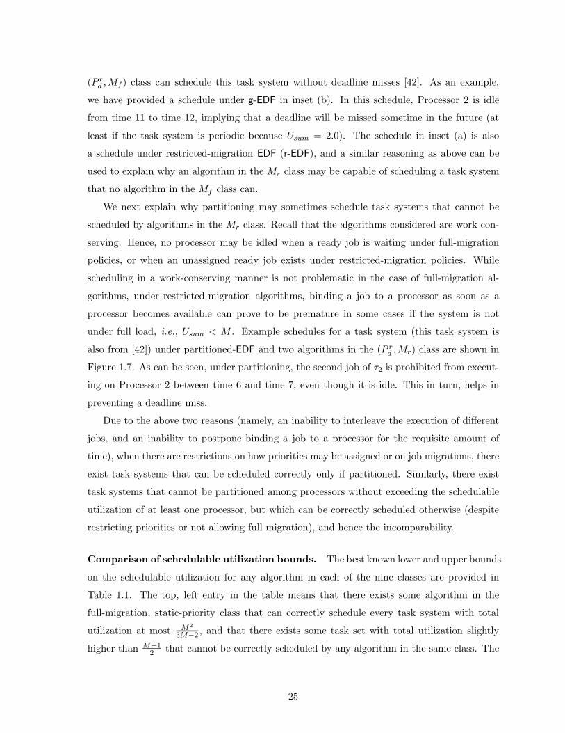
(P rd ,Mf ) class can schedule this task system without deadline misses [42]. As an example,

we have provided a schedule under g-EDF in inset (b). In this schedule, Processor 2 is idle

from time 11 to time 12, implying that a deadline will be missed sometime in the future (at

least if the task system is periodic because Usum = 2.0). The schedule in inset (a) is also

a schedule under restricted-migration EDF (r-EDF), and a similar reasoning as above can be

used to explain why an algorithm in the Mr class may be capable of scheduling a task system

that no algorithm in the Mf class can.

We next explain why partitioning may sometimes schedule task systems that cannot be

scheduled by algorithms in the Mr class. Recall that the algorithms considered are work con-

serving. Hence, no processor may be idled when a ready job is waiting under full-migration

policies, or when an unassigned ready job exists under restricted-migration policies. While

scheduling in a work-conserving manner is not problematic in the case of full-migration al-

gorithms, under restricted-migration algorithms, binding a job to a processor as soon as a

processor becomes available can prove to be premature in some cases if the system is not

under full load, i.e., Usum < M . Example schedules for a task system (this task system is

also from [42]) under partitioned-EDF and two algorithms in the (P rd ,Mr) class are shown in

Figure 1.7. As can be seen, under partitioning, the second job of τ2 is prohibited from execut-

ing on Processor 2 between time 6 and time 7, even though it is idle. This in turn, helps in

preventing a deadline miss.

Due to the above two reasons (namely, an inability to interleave the execution of different

jobs, and an inability to postpone binding a job to a processor for the requisite amount of

time), when there are restrictions on how priorities may be assigned or on job migrations, there

exist task systems that can be scheduled correctly only if partitioned. Similarly, there exist

task systems that cannot be partitioned among processors without exceeding the schedulable

utilization of at least one processor, but which can be correctly scheduled otherwise (despite

restricting priorities or not allowing full migration), and hence the incomparability.

Comparison of schedulable utilization bounds. The best known lower and upper bounds

on the schedulable utilization for any algorithm in each of the nine classes are provided in

Table 1.1. The top, left entry in the table means that there exists some algorithm in the

full-migration, static-priority class that can correctly schedule every task system with total

utilization at most M2

3M−2 , and that there exists some task set with total utilization slightly

higher than M+12 that cannot be correctly scheduled by any algorithm in the same class. The

25

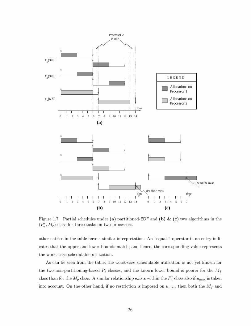
τ (3,6)1

τ (3,6)2

τ (6,7)3



L E G E N D

0 1 2 3 4 5 6 7 8 9 10 11 12 13 14

time

Processor 2 is idle

0 1 2 3 4 5 6 70 1 2 3 4 5 6 7 8 9 10 11 12 13 14

time timedeadline miss

deadline miss

(a)

(b) (c)

Figure 1.7: Partial schedules under (a) partitioned-EDF and (b) & (c) two algorithms in the(P r

d ,Mr) class for three tasks on two processors.

other entries in the table have a similar interpretation. An “equals” operator in an entry indi-

cates that the upper and lower bounds match, and hence, the corresponding value represents

the worst-case schedulable utilization.

As can be seen from the table, the worst-case schedulable utilization is not yet known for

the two non-partitioning-based Ps classes, and the known lower bound is poorer for the Mf

class than for the Mp class. A similar relationship exists within the P rd class also if umax is taken

into account. On the other hand, if no restriction is imposed on umax, then both the Mf and

26

Mp classes within the P rd class have identical worst-case schedulable utilizations. In general,

it appears that all the three migration sub-classes have comparable schedulable utilizations

when taken within either the static- or restricted-dynamic-priority classes. Further, as can be

seen from the table, the schedulable utilizations of these classes cannot exceed M+12 (which

is roughly 50%) in the worst case. However, in sharp contrast to these two priority classes,

easing the restrictions on migrations can increase schedulability to 100% under the unrestricted

dynamic-priority class.

Comparison of preemption and migration overheads. Unlike schedulability, which,

contrary to normal expectations, does not always improve as migrations are more liberally

allowed, run-time overhead generally increases as the migration rules become more general.

Some significant components of the overhead imposed by migration are discussed below. But

first, a general description of the memory hierarchy present in computers is in order.

Modern computers are provided with a memory hierarchy to speed up accesses to memory

references that exhibit spatial or temporal locality. Registers and different levels of caches

are above the main memory in this hierarchy and are local to processors. Access times are

longer to storage elements lower down in the hierarchy, and since an address is likely to be

available at different levels at different times, not all accesses to a given address will have the

same access time at all times or from all processors. The differences among the access times to

registers and different cache levels are generally negligible compared to the difference between

the access times to the lowest-level cache and the main memory. Hence, we will let the term

cache refer collectively to all storage above main memory.

The presence of a memory hierarchy immediately suggests that a job will complete execut-

ing sooner if its memory requests can be served from the cache. Spatial and temporal locality

exhibited by the memory-access requests of most programs suggests that it is more likely for

such requests of a job to be served from the cache, if the job executes on a single processor and

without preemptions. Thus, a major overhead due to migrations is that due to a loss of cache

affinity, i.e., the time needed to fetch the contents of addresses that would have otherwise

been serviced in-cache, from main memory. With write-back13 caches, this overhead includes

the time needed to invalidate associated cache lines, if needed, on the first processor (i.e., the

13Caches generally use one of the two policies for updating memory: write-through and write-back . In write-through caches, any write to an address is to both the cache and the memory, whereas in write-back caches, awrite to memory is deferred until the associated cache line is replaced or the contents are needed by some otherprocessor.

27

processor that the job executed upon prior to preemption) apart from the time needed to fetch

the contents from that processor’s cache or the main memory. Another significant component

of the migration overhead is the time needed to invalidate the cache lines containing a job’s

process control block (PCB) from the first processor’s cache (if it is dirty), refetch it into the

cache of the second processor, and load needed process status registers. On modern processors

with support for virtual memory, recently-used page table entries of a process may also have

to be invalidated and refetched.

Note that some of the overheads described above can be incurred even if a preempted job

resumes execution at a later time on the same processor, that is, even if a job is only preempted

but does not migrate. The amount of overhead will depend on whether its cache lines were

evicted by jobs that executed in the intervening time. Since the state of the cache cannot be

predicted reliably, it is common to assume a cold cache as the worst case even for preemptions.

However, in practice, cache-related overheads are likely to be more pronounced if a job really

migrates, and hence overhead due to migration also increases with increased generalization.

The crux of the comparison of the priority and migration classes presented above and

in Section 1.4.2.1 can be stated as follows. Increased generalizations along the priority and

migration dimensions come at a price that may be acceptable if the gain in schedulability that

the generalization enables outweighs the loss it imposes due to overheads.

The loss incurred as we move from static-priority schedulers to restricted-dynamic-priority

schedulers due to the overheads of more complex scheduling should be negligible on modern

systems (and perhaps even on systems that are less powerful) in comparison to the increase in

schedulability. As discussed in Section 1.4.2.1, for some task systems, moving to a restricted-

dynamic-priority scheduler can in fact lower the number of preemptions, leading to an overall

decrease in the loss due to overheads. Hence, in this dissertation, we consider only the two

dynamic-priority categories. We close this section by summarizing the trade-offs between

flexibility and overheads offered by increasing migration within dynamic-priority categories.

1.4.2.3 Overheads versus Flexibility Trade-offs

Though migrations and preemptions can add to the overheads incurred, allowing them im-

proves a scheduler’s flexibility, and can help in meeting more timing constraints in real-time

systems. Recall that the full-migration, unrestricted-dynamic-priority class is more power-

ful than every other class. Furthermore, if migrations are prohibited, then tasks have to be

partitioned among the available processors. Though cache-related overheads are the least

28

with partitioning, this method suffers from two significant drawbacks. First, task partitioning

should ensure that no processor’s capacity is exceeded, and so is a bin-packing problem,14

which is NP-hard in the strong sense [59]. Hence, determining an optimal task assignment is

intractable except for very small task systems, and sub-optimal heuristics are commonly used.

Second, partitioning may be a cumbersome strategy in dynamic15 task systems, in which task

composition, i.e., the set of tasks and/or their utilizations can change at run-time, invalidating

the current partitioning and necessitating a repartitioning. The worst-case time complexity

of commonly-used partitioning heuristics is at least O(NM), and hence, partitioning can be

prohibitive to perform at run-time. Furthermore, if repartitioned, tasks have to migrate, and

the prime benefit of partitioning, namely, lack of migrations and processor affinity for tasks,

is lost.

Apart from the above drawbacks of partitioning, recent trends and developments in pro-

cessor and computer architecture have led to designs that can considerably mitigate migration

overheads, and hence, augur well for global scheduling algorithms. One significant trend is

the emergence of multicore architectures, which have multiple processing units on a single

die. It is widely believed that multicore architectures are the way to achieve higher processor

performance, given that thermal and power problems impose limits on the performance that

a single processing unit can deliver. In some multicore-based designs, the different processor

cores share one or more levels of on- or off-chip caches. Hence, tasks do not significantly lose

cache affinity when they migrate, and so, overheads due to migration are rendered almost

negligible.

Thus, as things currently stand, no class is clearly superior than the rest, and it can be

expected that the choice of the algorithm depends on the characteristics of the underlying

platform and the application at hand. However, as shown in Figure 1.1(a), pure partitioning

has no scope of improving system utilization if a task system cannot be partitioned among

the available processors, even if bounded tardiness is tolerable. Hence, since our focus in this

dissertation is soft real-time systems, we do not consider no-migration algorithms. As already

discussed, we do not consider static-priority algorithms either. Thus, our focus is restricted to

the upper, right (2 × 2) sub-matrix of Table 1.1.

14Here, processors are the bins, tasks are items to be packed, schedulable utilizations of the processors’scheduling algorithms are the bin sizes, and task utilizations are item sizes.

15There is no relation between dynamic task systems and dynamic priorities. A dynamic task system can bescheduled by a static-priority scheduling algorithm.

29

With the above introduction to real-time systems and associated concepts, and hard real-

time scheduling on multiprocessors in place, we are ready to describe soft real-time systems

next.

1.5 Soft Real-Time Systems

As mentioned in Section 1.1, violations of soft real-time constraints are not disastrous and

can be tolerated occasionally or by bounded amounts. A task with soft (resp., hard) real-

time constraints is said to be a soft (resp., hard) real-time task . A real-time system may

either consist exclusively of either hard real-time tasks or soft real-time tasks only, or be a

combination of the two. As a simple example, consider a radar tracking system tracking both

hostile and friendly targets. In such a system, deadlines of tasks that track hostile targets must

not be missed, whereas those of tasks that track friendly targets may be missed by bounded

amounts.

It should be noted that the definition of soft real-time is somewhat broad and can span a

wide spectrum of systems. The nature and extent of violations of timing constraints permissi-

ble for soft real-time tasks is application dependent. Determining permissible levels of violation

is beyond the scope of this dissertation and it is assumed that such levels are provided. Some

significant soft real-time models proposed in the literature that differ in the nature of permis-

sible violations are reviewed in Chapter 2. Below, we merely describe the model considered in

this dissertation.

Soft real-time task model. The soft real-time task model that we consider augments the

sporadic and periodic task models described in Section 1.3 by associating a tardiness threshold

with every task in the task system. If δ denotes the tardiness threshold of a soft real-time

task, then any job of the task can be late, i.e., miss its deadline, by at most δ time units.

Though there exist task systems composed of tasks with different tolerances to tardiness, in

this dissertation we restrict our attention primarily to systems whose tasks have equal tolerance

to tardiness.

Formally, the tardiness of a job Ti,j in schedule S is defined as tardiness(Ti,j,S) = max(0, t−di,j), where t is the time at which Ti,j completes executing in S. The tardiness of a task system

τ under scheduling algorithm A, denoted tardiness(τ,A), is defined as the maximum tardiness

of any job of any task in any schedule for any concrete instantiation of τ under A. If under

30

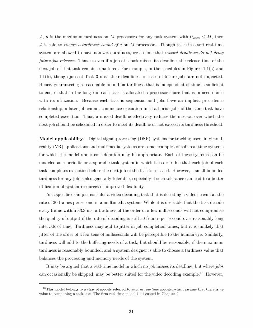
A, κ is the maximum tardiness on M processors for any task system with Usum ≤ M , then

A is said to ensure a tardiness bound of κ on M processors. Though tasks in a soft real-time

system are allowed to have non-zero tardiness, we assume that missed deadlines do not delay

future job releases. That is, even if a job of a task misses its deadline, the release time of the

next job of that task remains unaltered. For example, in the schedules in Figures 1.1(a) and

1.1(b), though jobs of Task 3 miss their deadlines, releases of future jobs are not impacted.

Hence, guaranteeing a reasonable bound on tardiness that is independent of time is sufficient

to ensure that in the long run each task is allocated a processor share that is in accordance

with its utilization. Because each task is sequential and jobs have an implicit precedence

relationship, a later job cannot commence execution until all prior jobs of the same task have

completed execution. Thus, a missed deadline effectively reduces the interval over which the

next job should be scheduled in order to meet its deadline or not exceed its tardiness threshold.

Model applicability. Digital-signal-processing (DSP) systems for tracking users in virtual-

reality (VR) applications and multimedia systems are some examples of soft real-time systems

for which the model under consideration may be appropriate. Each of these systems can be

modeled as a periodic or a sporadic task system in which it is desirable that each job of each

task completes execution before the next job of the task is released. However, a small bounded

tardiness for any job is also generally tolerable, especially if such tolerance can lead to a better

utilization of system resources or improved flexibility.

As a specific example, consider a video decoding task that is decoding a video stream at the

rate of 30 frames per second in a multimedia system. While it is desirable that the task decode

every frame within 33.3 ms, a tardiness of the order of a few milliseconds will not compromise

the quality of output if the rate of decoding is still 30 frames per second over reasonably long

intervals of time. Tardiness may add to jitter in job completion times, but it is unlikely that

jitter of the order of a few tens of milliseconds will be perceptible to the human eye. Similarly,

tardiness will add to the buffering needs of a task, but should be reasonable, if the maximum

tardiness is reasonably bounded, and a system designer is able to choose a tardiness value that

balances the processing and memory needs of the system.

It may be argued that a real-time model in which no job misses its deadline, but where jobs

can occasionally be skipped, may be better suited for the video decoding example.16 However,

16This model belongs to a class of models referred to as firm real-time models, which assume that there is no

value to completing a task late. The firm real-time model is discussed in Chapter 2.

31

this model may have the disadvantage that optimally determining whether to skip a frame

can incur additional scheduling overhead at run-time. This is because not too many frames

can be skipped from the same stream and every frame that is not skipped should meet its

deadline. Further, to our knowledge, no experimental evidence is available as to which is a

better approach, and it appears that if tardiness is minimal, then it may actually be preferable

to not skip frames. Also, if the video stream is MPEG-coded, then it may not be possible

to skip frames arbitrarily. Specifically, since the I and P frames are needed in decoding B

frames and other P frames, there is less freedom in choosing frames to skip. In the case of

DSP systems, since the accuracy of the computational results on a later sample increases if the

results of processing the most recent sample are available, there is value to completing tasks

as long as they are not too late.

A final argument in support of the model of interest to us is as follows. As discussed in

Chapter 2, almost all the work on the other soft real-time models considered in the literature

is with respect to uniprocessors and is concerned with dealing with overload, i.e., scenarios

in which the total system utilization exceeds the available utilization, which is 1.0. Overload

could be over long terms, such as system lifetime, or occasional and for short durations, as

in systems whose average loads do not exceed the available capacity but whose instantaneous

loads could exhibit significant variations. However, in the context of multiprocessors, there

exist scheduling algorithms under which guarantees on timeliness that can be provided are

not known when the total utilization exceeds the schedulable utilization (i.e., U(M)) of the

algorithm, but is much lower than the total available capacity (i.e., M), i.e., even when the

system is much below full load. This is true of all the algorithms in Table 1.1, except the

optimal algorithms, which belong to the (P ud ,Mf ) class, necessitating a study of the model.

We conjecture that results based on the model considered may, in fact, be necessary in dealing

with overload.

With needed background and concepts in place, we return to the subject of this dissertation,

namely, facilitating cost-effective implementations of soft real-time systems on multiprocessors.

We begin by articulating a need for research in this direction.

1.6 Limitations of State-of-the-Art

As noted in Section 1.2.2, the current multiprocessor-based real-time scheduling theory is too

expensive for direct application to soft real-time systems. Below, we briefly explain why this

32

is the case.

Deficiencies of non-optimal algorithms. A necessary and sufficient condition for the

feasibility of a recurrent task system τ on M processors is that Usum(τ) ≤ M hold [25, 14].

(As explained in Section 1.3.3, Usum17 denotes the total system utilization after accounting for

all the run-time overheads including scheduling, context-switching, preemption, and migration

overheads.) From the discussion in Section 1.4.2.2 of the entries in Table 1.1, it is known

that algorithms in eight of the nine classes (i.e., all the classes except the (P rd ,Mf ) class) are

not optimal, and require restrictions on total system utilization that can approach roughly

50% of the available processing capacity if every deadline needs to be met. Hence, when

bounded tardiness is tolerable, using the utilization bounds given in Table 1.1 for validation

with algorithms in those classes can be overkill. Furthermore, it is possible that new algorithms

(algorithms not studied in the context of hard real-time systems) are better suited for soft real-

time systems (even though their schedulable utilizations are guaranteed to not exceed 50%).

Deficiencies of optimal algorithms. It also follows from the same table that there exist

algorithms in the (P ud ,Mf ) class that are optimal, implying that the underlying system need

not be underutilized. All known optimal algorithms in this class fall under a subclass called

proportionate-fair or Pfair [25] scheduling algorithms. Nevertheless, the use of optimal Pfair

algorithms can be overkill as well for soft real-time systems for the following reasons.

Quantum-based scheduling: Optimal Pfair algorithms are quantum based , i.e., schedule

tasks one quantum at a time, and as a result, the scheduler is invoked more often and

tasks are prone to frequent preemptions and migrations. Hence, the effective system

utilization, after accounting for the overheads as explained in Section 1.3.3, can be much

less than 100%.

Integer execution costs and periods: Optimal Pfair algorithms require the execution costs

and periods of tasks to be specified as integer multiples of the quantum size. Hence, when

non-integral, execution costs have to be rounded up and periods have to be rounded down.

For some task systems, the associated loss to effective system utilization can be quite

significant.

17We will omit specifying the task system as a parameter when unambiguous.

33

Apart from the above restrictions, which can lead to a significant loss of effective system

utilization, optimal Pfair algorithms impose some other restrictions also, which can limit their

practical implementation and can be problematic for soft real-time systems. Hence, it is

desirable that such restrictions, which are described below, be relaxed (apart from relaxing

the two restrictions above).

Synchronized scheduling: To ensure optimality, optimal Pfair algorithms require that tasks

be allocated processor time in fixed-sized quanta that align across all processors. Apart

from posing implementation challenges, this requirement can also lead to wasted proces-

sor time in that when a task executes for less than its WCET and yields in the middle

of a quantum, or blocks on a lock request in the middle of a quantum, the associated

processor idles for the remainder of the quantum. This waste of processor time could po-

tentially be eliminated for soft real-time systems if bounded tardiness can be guaranteed

by a simpler algorithm in which the aligned-quanta restriction is relaxed.

Tie-breaking rules: Optimal algorithms require non-trivial tie-breaking rules to resolve ties

among subtasks18 with the same deadline. Such rules may be unnecessary or unaccept-

able for soft and dynamic real-time systems. Hence, identifying the timeliness properties

of algorithms that use no tie-breaking rules can enhance the applicability of Pfair algo-

rithms for such systems.

Based on the limitations of optimal and non-optimal algorithms described above, we con-

clude that the known scheduling algorithms and/or validation tests in all the nine categories

are rigid and can be overkill for soft real-time systems. Furthermore, we believe that there is

sufficient scope to improve system utilization and implementation support for soft real-time

systems on multiprocessors by (i) developing new validation tests specifically for soft real-time

systems, (ii) relaxing some of the limiting restrictions of the optimal Pfair algorithms and

deriving the timing properties of the resulting simpler algorithms, and (iii) designing new

algorithms tailored for soft real-time systems. Accordingly, the thesis of this dissertation is as

follows.

Thesis Statement: Processor utilization can be improved on multiprocessors while

ensuring non-trivial soft real-time guarantees for different soft real-time applica-

tions whose preemption and migration overheads can span different ranges and

18In Pfair terminology, each quantum’s worth of execution is referred to as a subtask. Refer to Chapter 3 fora more formal definition.

34

whose tolerances to tardiness are different by designing new scheduling algorithms,

simplifying optimal ones, and developing new validation tests.

Our contributions in support of the above thesis are described below.

1.7 Contributions

We establish our thesis as follows. We analyze two known algorithms, one new algorithm, and

some simpler Pfair algorithms that are non-optimal but less expensive than optimal algorithms

to determine their soft real-time guarantees. Specifically, for each algorithm A that we analyze,

we determine the guarantees on timeliness that A can provide if the total system utilization,

Usum, exceeds the schedulable utilization, UA(M), of A, but not the total available capacity,

M , of the underlying system. In the known algorithms category, we show that both global

preemptive EDF (i.e., g-EDF) and global non-preemptive EDF (i.e., g-NP-EDF) can guarantee

very reasonable, bounded tardiness in most cases. With respect to Pfair algorithms, we show

that simpler algorithms that relax one or more of the limiting restrictions described in Sec-

tion 1.6 that are needed for optimality can guarantee small, bounded tardiness. Finally, we

design and analyze a new partitioning-based, restricted-migration algorithm called EDF-fm,

which limits the number of tasks that need to migrate, and derive tardiness bounds under it.

The algorithms considered differ in the degree of preemptions and migrations they require,

and hence, can benefit different applications that differ in their preemption and migration

costs. That is, system utilization levels can be improved for different applications whose

overheads span different ranges if they can tolerate bounded tardiness. Similarly, since the

algorithms considered differ in the tardiness bounds they can guarantee, different applications

with different tardiness thresholds can benefit, as well. Finally, as Block et al. show in [36],

[35], and [37], the algorithms in the different classes differ in how quickly they can adapt to

run-time changes in task composition, i.e., how suitable they are for dynamic task systems.

Determining when and how to adapt within any algorithm is quite complex and is beyond

the scope of this dissertation. However, in soft real-time systems, rules for adapting to run-

time changes require some basic results on timeliness guarantees, which we determine in this

research. Thus, the results of this dissertation can enable different applications that differ in

the adaptivity they require.

The results we have obtained for soft real-time systems are summarized in Table 1.2 and

are discussed in more detail below.

35

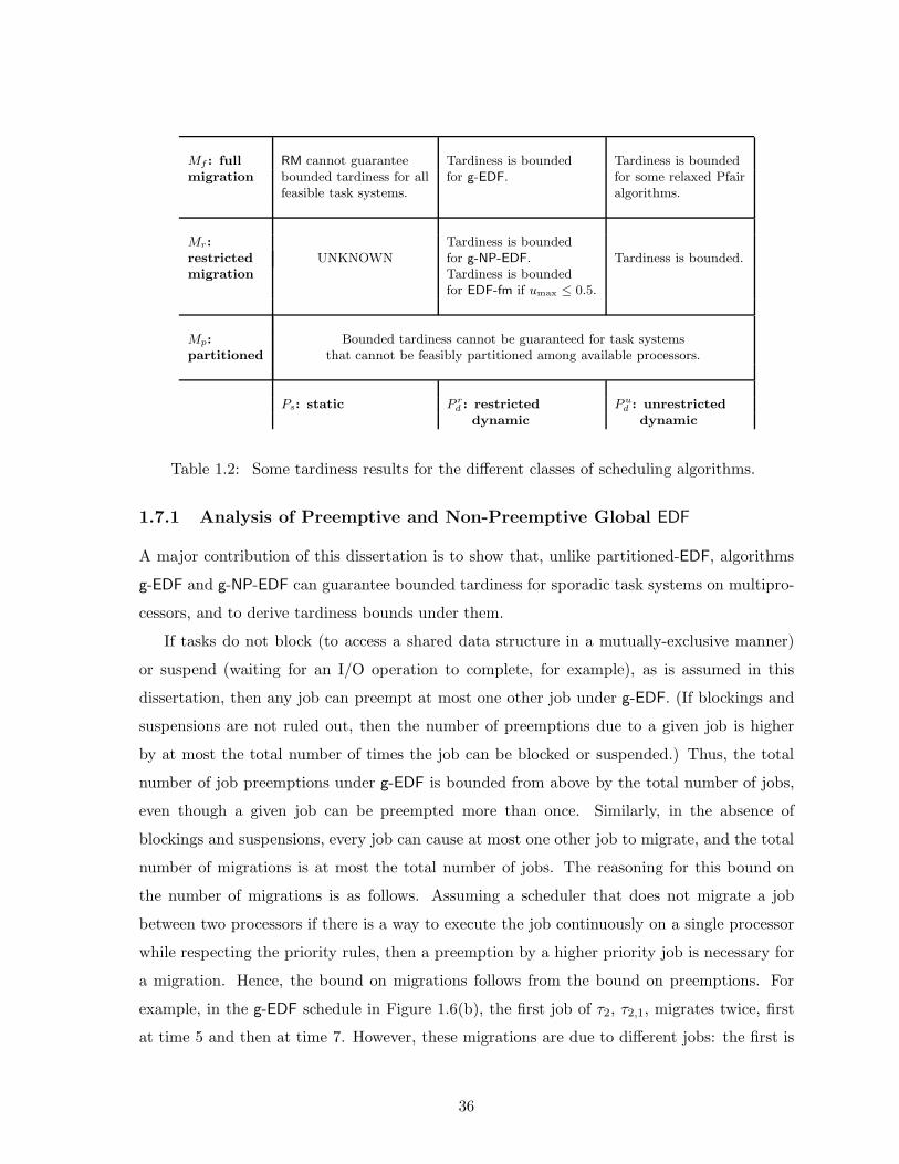
Mf : full RM cannot guarantee Tardiness is bounded Tardiness is boundedmigration bounded tardiness for all for g-EDF. for some relaxed Pfair

feasible task systems. algorithms.

Mr: Tardiness is boundedrestricted UNKNOWN for g-NP-EDF. Tardiness is bounded.migration Tardiness is bounded

for EDF-fm if umax ≤ 0.5.

Mp: Bounded tardiness cannot be guaranteed for task systemspartitioned that cannot be feasibly partitioned among available processors.

Ps: static P rd : restricted P u

d : unrestricted

dynamic dynamic

Table 1.2: Some tardiness results for the different classes of scheduling algorithms.

1.7.1 Analysis of Preemptive and Non-Preemptive Global EDF

A major contribution of this dissertation is to show that, unlike partitioned-EDF, algorithms

g-EDF and g-NP-EDF can guarantee bounded tardiness for sporadic task systems on multipro-

cessors, and to derive tardiness bounds under them.

If tasks do not block (to access a shared data structure in a mutually-exclusive manner)

or suspend (waiting for an I/O operation to complete, for example), as is assumed in this

dissertation, then any job can preempt at most one other job under g-EDF. (If blockings and

suspensions are not ruled out, then the number of preemptions due to a given job is higher

by at most the total number of times the job can be blocked or suspended.) Thus, the total

number of job preemptions under g-EDF is bounded from above by the total number of jobs,

even though a given job can be preempted more than once. Similarly, in the absence of

blockings and suspensions, every job can cause at most one other job to migrate, and the total

number of migrations is at most the total number of jobs. The reasoning for this bound on

the number of migrations is as follows. Assuming a scheduler that does not migrate a job

between two processors if there is a way to execute the job continuously on a single processor

while respecting the priority rules, then a preemption by a higher priority job is necessary for

a migration. Hence, the bound on migrations follows from the bound on preemptions. For

example, in the g-EDF schedule in Figure 1.6(b), the first job of τ2, τ2,1, migrates twice, first

at time 5 and then at time 7. However, these migrations are due to different jobs: the first is

36

due to τ3,2 and the second, due to τ1,3. Thus, because of a moderate number of migrations,

g-EDF could be a good choice for applications with moderate migration costs. As discussed

in Section 1.4.2.3, partitioning may not be acceptable for highly dynamic task systems even

if migration costs are high. The tardiness bound that we have derived under g-EDF on M

processors for task Tk of a task system τ with Usum ≤ M is given by

∑Λi=1 εi − emin

M −∑Λ−1i=1 µi

+ ek.

(Refer to Section 4.2 for formal definitions of εi, µi, and Λ. Λ is approximately Usum−1 and εi

(resp., µi) is the ith highest execution cost (resp., utilization) of any task in τ .) As discussed

in detail in Chapter 4, the above bound is reasonable unless task utilizations and the number

of processors M are both high.

The tardiness bound derived under g-NP-EDF is given by

∑Λ+1i=1 εi − emin

M −∑Λi=1 µi

+ ek,

which is higher than that derived under g-EDF given above. Recall that g-NP-EDF is a

restricted-migration algorithm, hence despite being subject to a higher tardiness bound, the

algorithm may be preferable when the cost of migrating any given job is high, but not much

state is associated with a task itself that is carried between its jobs. Also, on each processor,

at most one job may be in a started but unfinished state, and hence, g-NP-EDF has the added

benefit of lowering the total stack size, which may especially be desirable in embedded systems.

Finally, implementing g-NP-EDF on an SMP is likely to be much simpler than implementing

g-EDF, and our experience in implementing these algorithms within the Linux kernel as part

of the LITMUSRT [41] project confirms this. Refer to Chapter 9 for more details.

1.7.2 Design and Analysis of EDF-fm

As a second contribution, we design an algorithm based on partitioned-EDF, called EDF-fm, for

use with applications with high inter- and intra-job migration costs. A pure partitioning algo-

rithm (i.e., a no-migration algorithm), offers no scope for guaranteeing bounded tardiness, and

hence, for improving processor utilization, for soft real-time systems that cannot be partitioned

among the available processors. Thus, migrations are necessary in such systems. Hence, in

designing EDF-fm, our focus was on minimizing required migrations only to the extent needed

37

for guaranteeing bounded tardiness. Specifically, under EDF-fm, on an M -processor system,

the capability to migrate is required for at most M − 1 tasks, and it is sufficient that every

such task migrates between two processors and at job boundaries only.

1.7.3 Analysis of Non-Optimal, Relaxed Pfair Algorithms

Our third contribution is in determining the timeliness properties of some simpler Pfair algo-

rithms.

Pfair algorithms, which schedule tasks one quantum at a time, may be better suited than

EDF for applications with low-migration costs and lower tolerance to tardiness. However, as

discussed in Section 1.6, the scheduling and task model restrictions imposed by Pfair scheduling

can lower its effective utilization and limit its practical implementation. In an attempt to

enhance the applicability of Pfair scheduling for soft real-time systems, we considered relaxing

some of those restrictions.

Tie-breaking rules. The earliest-pseudo-deadline-first (EPDF) Pfair scheduling algorithm [15]

is a non-optimal algorithm, which uses no tie-breaking rules and resolves ties among subtasks

arbitrarily. The appropriateness of EPDF for soft real-time systems was first considered by

Srinivasan and Anderson in [106], where they derived sufficient per-task utilization restrictions

for ensuring bounded tardiness under EPDF. However, they left some questions unanswered.

We have answered a few of those questions by extending the existing validation analysis for

EPDF in the following ways. First, we show that the prevailing conjecture that EPDF can en-

sure a tardiness bound of one quantum for all feasible task systems in false. Next, we improve

Srinivasan and Anderson’s sufficient per-task utilization restrictions for guaranteeing bounded

tardiness under EPDF. Third, we derive non-trivial sufficient restrictions along an orthogonal

dimension, namely, total system utilization, for schedulability under EPDF, thereby extend-

ing the applicability of EPDF for hard real-time systems. Finally, we consider extending the

restriction on total system utilization to allow bounded tardiness.

Synchronized scheduling. Elsewhere [50], we have considered relaxing the synchronized

scheduling requirement of Pfair algorithms, which, as discussed in Section 1.6, requires tasks

to be allocated processor time in fixed-sized quanta that align on all processors. We show that

if scheduling is desynchronized , then under an otherwise-optimal Pfair scheduling algorithm,

deadlines are missed by at most the maximum size of one quantum. Further, we argue that

38

this result can be extended to most prior results on Pfair scheduling: in general, tardiness

bounds guaranteed under EPDF and other sub-optimal Pfair algorithms are worsened by at

most one quantum when scheduling is desynchronized.

Integer execution costs and periods and quantum-based scheduling. We use part

of the analysis used in deriving the timing properties of desynchronized Pfair algorithms to

show that if periods are non-integral, but execution costs are still integral, then deadlines can

be missed by less than two quanta. Finally, to mitigate the loss to total system utilization

due to quantum-based scheduling when migration costs are high or execution costs are non-

integral, we propose a technique based on job slicing. This job-slicing technique obviates the

need to round execution costs up, can lower migration overheads, and can guarantee small and

bounded tardiness.

1.7.4 Implementation Considerations and Evaluation of Algorithms

As noted earlier, the performance of each algorithm considered in this dissertation depends

on the characteristics of the underlying platform and the application at hand. To better

perceive the overheads versus schedulability trade-off offered by the various algorithms, we

present a simulation-based evaluation of the algorithms using overheads measured on a real

test bed and soft real-time schedulability tests. Our evaluation methodology is as follows. We

first identify significant sources of external overhead that can delay application tasks, and for

each algorithm, provide formulas for computing inflated WCETs for tasks that are sufficient

to account for all the overheads. Next, we measure typical values for each overhead on a real

test bed, which, in our case, is LITMUSRT, running on a 4-processor SMP [41]. We finally

use the measured overhead costs in simulation-based experiments to compute inflated WCETs,

schedulability (in a soft real-time sense), and tardiness bounds under the various algorithms

considered in this dissertation and under partitioned-EDF for randomly-generated task sets.

Our metrics for comparison are the percentage of task systems to which each algorithm can

guarantee bounded tardiness and the mean of the maximum tardiness bound guaranteed. For

each algorithm, we also discuss scenarios in which it may be the best choice, and briefly

comment on efficient implementation techniques.

39

1.8 Organization

The rest of this dissertation is organized as follows. Chapter 2 reviews prior work on soft

real-time scheduling. Chapter 3 reviews Pfair scheduling in detail and presents needed no-

tation. Tardiness bounds under preemptive and non-preemptive global EDF are derived in

Chapter 4. In Chapter 5, algorithm EDF-fm and associated analyses for soft real-time systems

are presented. A schedulable utilization bound under the EPDF Pfair scheduling algorithm and

improved sufficient restrictions on per-task utilizations for bounded tardiness under it are then

derived in Chapters 6 and 7, respectively. Supporting non-integral execution costs and periods

is considered in Chapter 8, while implementation considerations and a performance evaluation

of the concerned algorithms are presented in Chapter 9. Chapter 10 concludes with a summary

of the work presented in this dissertation and an enumeration and discussion of some issues

that remain to be addressed in the area of soft real-time scheduling on multiprocessors.

40

Chapter 2

Related Work

In this chapter, prior work on soft real-time systems is surveyed. Work related to the multi-

processor scheduling algorithms considered in this dissertation is discussed in later chapters.

As discussed in Chapter 1, violations of soft real-time constraints are neither disastrous

nor desirable, and can be tolerated if they are occasional, or are by bounded amounts. This

definition by itself is hardly useful in designing real systems unless the terms “occasional” and

“bounded” are precisely specified. Also, if timing constraints can be weakened, then there are

different possibilities for doing so, each of which may be more appropriate for some applications

than others. Accordingly, several soft real-time models that differ in the nature and extent of

violations they allow have been proposed. We will classify such models as either deterministic

or probabilistic based on the predominant nature of the specifications in the model and the

type of soft real-time guarantees they provide.

Firm real-time. One type of a non-hard real-time task is a firm real-time task. A firm

real-time task is one whose deadline misses are not disastrous, but whose results are not useful

when late. Thus, it is preferable to not execute a job of a firm real-time task whose deadline

will not be met. We will treat a firm real-time task as a special type of a soft real-time task

though the two are sometimes considered to be distinct in the literature. Our survey includes

models for firm real-time tasks as well.

This chapter is organized as follows. It begins with a survey of deterministic models in

Section 2.1. Probabilistic models are considered next in Section 2.2, followed by a discussion

of time-value functions in Section 2.3. Time-value functions are not included in Section 2.1 or

Section 2.2 because the stated objective of scheduling based on such functions is quite different

from those of models considered in these earlier sections. Also, for the general time-value func-

tion model, scheduling is predominantly best effort and guarantees are rarely provided.1 The

chapter concludes by enumerating prior work on multiprocessor-based soft real-time schedul-

ing.

2.1 Deterministic Models for Soft Real-Time Systems

In this section, some deterministic soft real-time task models are described. Algorithms for

scheduling task systems specified using those models and associated analyses are also described

where needed. Unless otherwise specified, all of the work described pertains to uniprocessors.

2.1.1 Skippable Task Model

Among the early deterministic models is the skippable periodic/sporadic task model of Koren

and Shasha [73]. In this model, a job of a task may be skipped , i.e., may not execute at all

or have its execution aborted mid-way, as long as there is a minimum separation, referred to

as the task’s skip parameter , between consecutive skips. Task τi’s skip parameter is denoted

si, where si ≥ 2, and has the interpretation that for every job of τi that is skipped, at least

si − 1 following jobs are not to be skipped. Using Koren and Shasha’s terminology, a job that

may be skipped is said to be blue, and one that has to complete by its deadline, red . This

model was developed to support some signal-processing systems, where some samples can be

skipped, and streaming applications that are tolerant to packet losses.

Let URdef=

∑Ni=1

ei·(si−1)pi·si

denote the total utilization considering only jobs that may not

be skipped. One might reasonably expect that UR ≤ 1 is a sufficient feasibility condition.

However, consider the task system τ = {τ1(3.5, 4), τ2(1, 4)}. Clearly, this task system is not

feasible on a uniprocessor if no job of any task may be skipped. It is also not feasible if only

jobs of τ1 may be skipped regardless of the value of τ1’s skip parameter, s1. (Note that s1

should be at least two.) This is because if both τ1 and τ2 release a red job each at the same

time, then at most one can complete execution by its deadline. For this example, with s1 = 2,

i.e., when every other job of τ1 may be skipped, UR = 3.58 + 1

4 = 5.58 , which is less than 1.0.

Hence, UR ≤ 1 is not a sufficient condition for ensuring the feasibility of a skippable task

system.

1It should be noted that algorithms with provable properties have been developed for some very specialcases [28] and providing probabilistic guarantees has been considered in some recent work [79].

42

τ2(3,4)

τ1(3,4)

Red Red

0 2 4 6 8 0 2 4 6 8

Blue

Blue

Aborted

Blue

Blue

Red

Red Red

timetime

10 12

(b)(a)

Figure 2.1: Schedules for two concrete instances of a skippable sporadic task system.

As another example, task system τ = {τ1(3, 4), τ2(3, 4)} with s1 = s2 = 2 can be success-

fully scheduled. If τ is periodic, then a schedule in which odd jobs of τ1 and even jobs of τ2,

or vice versa, are skipped, would not violate any constraints. Note that for this task system,

UR = 38 + 3

8 = 34 , which is higher that the corresponding value for the previous example. Hence,

skippable task systems cannot be compared for feasibility based on their UR values.

Recall that the model allows jobs to be aborted mid-way and that an aborted job is also

considered to be a skipped job. Allowing such behavior may be necessary for sporadic task

systems because in such systems, whether a job is red or blue may have to be determined at

run-time, based on how jobs of other tasks are released. For illustration, let the task system in

the above example be sporadic and consider two partial sets of job releases as shown in insets

(a) and (b) of Figure 2.1. In each inset, at most one of τ1,1 and τ1,2 can meet its deadline

and τ1,1 is chosen for completion. Therefore, in each inset, τ2,2 is a red instance, and as far

as τ1 is concerned, τ1,2 is skippable, and hence, can be blue. Also, if τ1,2 is skipped, then τ1,3

would be a red instance, whose deadline must be met. τ1,3’s deadline can be met if τ2,2 is

released as in inset (a). On the other hand, if the release of τ2,2 is postponed as in inset (b)

and τ1,3 is released in time, then at most one of these two jobs can meet its deadline, leading

to a timing-constraint violation. However, this scenario can be avoided because τ2,2’s release is

sufficiently delayed that τ1,2’s deadline can be met and τ1,3 can be turned into a blue instance.

Therefore, when tasks are sporadic, schedulability can be improved by dynamically choosing

to not skip certain jobs.

43

It turns out that optimally determining which jobs to skip is NP-hard even if all job releases

are known a priori . Hence, Koren and Shasha proposed the use of algorithms based on simple

heuristics. In their first algorithm, called red tasks only (RTO), every (k · si)th job, for every

k ≥ 1, is considered blue, and is skipped. The remaining jobs are scheduled by either EDF

or RM. Note that the task system in the second example above is not schedulable by RTO,

even if it is periodic. Their second algorithm is called blue when possible (BWP), and tries to

provide improved service in comparison to RTO in a best-effort manner by scheduling some

blue job (chosen according to one of several heuristics) when no red job is pending. They also

provided associated schedulability conditions for both EDF and RM.

2.1.2 (m, k)-Firm Model

The (m,k)-firm model is similar to, and, in fact, subsumes the skippable task model, and was

proposed by Hamdaoui and Ramanathan [62].2 In this model, each task is associated with

two parameters m and k with the interpretation that at least m jobs in every window of k

consecutive jobs must meet their deadlines. Note that a skippable task with a skip parameter

s is also an (m,k)-task with parameters m = s − 1 and k = s, and that while every skippable

task can be represented as an (m,k) task the converse does not hold. Also, the (m,k) model

can allow skips to be consecutive, and in that sense, can provide weaker guarantees than the

skippable model.

Hamdaoui and Ramanathan proposed an algorithm called distance based priority (DBP)

for scheduling (m,k)-tasks. Unlike Koren and Shasha’s algorithms, scheduling under DBP is

dependent on run-time conditions. Hence, DBP maintains a state, which captures the current

history of met and missed deadlines, with each task. The task states are used to determine

how “unsafe” each task is, i.e., how close it is to having its (m,k) constraint violated, and

accord higher priority to tasks that are more unsafe. Tasks within the same priority class are

scheduled on an EDF basis.

The goal of DBP is to schedule tasks so that the average probability of violating the

(m,k) constraints is minimized and the realization of this goal is evaluated in [62] through

simulations. The model and the algorithm were initially developed for scheduling streams of

network packets, and hence, in the evaluations, the arrival pattern for jobs is neither periodic

nor sporadic, but is either Poisson or bursty. In [63], an analytic model of DBP that can be

2It appears that the skippable and (m, k) models were proposed at about the same time.

44

used to provide probabilistic guarantees on meeting the (m,k) constraint is developed, and its

accuracy is evaluated through simulations.

The application of the (m,k) model to overloaded periodic task systems is considered in

[98]. Here, as with RTO, static rules are provided for skipping jobs, and unskipped jobs are

scheduled using RM. A sufficient condition for deterministically meeting (m,k) constraints is

also derived.

2.1.3 Weakly-Hard Model

The weakly-hard model [32] has elements of both of the models described above and strives

to provide a general framework for the specification of soft real-time constraints. In [32],

soft real-time constraints are referred to as weakly-hard constraints. Currently, four types of

constraints, denoted(nm

)

,⟨ n

m

⟩

,(nm

)

, and⟨ n

m

⟩

, can be specified. The parameter m in all of

these expressions refers to any window of m consecutive jobs; parameter n refers to either the

number of met or missed deadlines. The(nm

)

specification is simply the (m,k) specification and

means that at least n jobs in any window of m consecutive jobs must meet their deadlines. This

is strengthened by⟨

nm

⟩

, which requires n consecutive deadlines to be met. The specifications

with overbars apply to the number of missed deadlines:(nm

)

means that fewer than n jobs

out of any consecutive m jobs may miss their deadlines;⟨ n

m

⟩

is a stronger specification under

which, out of m jobs, any number may be missed as long as fewer than n are consecutive.

In [32], the authors also developed an algebra of weakly-hard constraints that can allow

different types of constraints and constraints with different values for n and m to be related

and compared. They also discussed the possibility of associating multiple constraints with

each task. For instance, if a task can tolerate at most two misses in any window of four jobs,

but only at most eight misses (not ten) in a window of twenty jobs, then such a constraint can

be specified as(

24

)

∧(

820

)

.

Finally, the scheduling of weakly-hard real-time systems under static-priority algorithms

is considered. No special rules are included to improve the chances of meeting weakly-hard

constraints; rather, the objective is to determine whether a given system can meet all the con-

straints when scheduled using static priorities. This can be done in a straightforward manner

by using standard static-priority analysis for computing the response times3 of jobs released

3The response time of a job is given by the difference between the time the job completes executing and itsrelease time.

45

within a hyperperiod. The authors showed that neither the RM nor deadline-monotonic4 pri-

ority assignment is optimal for weakly-hard systems and discussed how to optimally assign

priorities.

2.1.4 Window-Constrained Model

The window-constrained model is a weaker variant of the (m,k)-firm model and was first consid-

ered in [119] and [118]. In this model, windows are non-overlapping in that every group of k jobs

from the beginning forms a window. In other words, in this model, jobs (k(i−1)+1), . . . , k · i,comprise the ith window, where i ≥ 1, whereas under the (m,k) model, jobs i, . . . , (i + k − 1)

form the ith window. The model parameters are specified as a pair (x, y) with the meaning that

at most x jobs in every non-overlapping window of y jobs may miss their deadlines. In [119]

and [118], an online algorithm called dynamic window-constrained scheduling was proposed for

scheduling packet streams with window constraints in communication networks. Conditions

for scheduling streams without violating the window constraints are also derived under the

assumption that packets are uniform in size and are non-preemptive.

The window-constrained model was subsequently studied by Mok and Wang [92], who

showed that, in general, determining whether a schedule that satisfies the window constraints

is possible is NP-hard in the strong sense. They also showed that some sub-classes of the

problem (such as those with unit execution costs, or are synchronous, periodic, or for which

x | y holds) can be solved efficiently, and devised scheduling algorithms and/or schedulability

tests for those sub-classes.

2.1.5 Imprecise Computation Model

The models discussed above allow some jobs to be treated as optional and their executions

to either complete late or be discarded entirely, as long as the optional jobs conform to the

constraint specification. The imprecise computation model takes a different approach: under

this model, some portion of each job may be discarded; however, in general, no job may be

discarded in its entirety or complete late. This model was proposed to allow graceful degrada-

tion during overload for tasks based on iterative algorithms such as numerical computations

or heuristic search, some multimedia tasks such as layered encoding and decoding, and others.

4 The deadline monotonic algorithm is a static-priority algorithm, which accords higher priority to taskswith shorter relative deadlines.

46

For such tasks, the quality of the results improves with the amount of time for which the jobs

execute; however, a certain minimum acceptable quality is reached when only a fraction of the

job completes execution. Hence, under this model each job of a task τi is logically decomposed

into two parts: a mandatory part, with execution cost emi, that corresponds to the minimum

required computation for the result to be acceptable, and an optional part, with execution

cost eoi, whose execution improves the quality of the results. The result produced by a job is

precise only if its mandatory and optional parts are both executed; otherwise, it is imprecise.

The optional part of each task is also associated with a reward function (or, correspondingly,

an error function), which is non-decreasing (resp., non-increasing) with respect to execution

time, and for a given time t, indicates the value (resp., penalty) that the system accrues by

executing (resp., not executing) the optional part of a job for t (resp., eoi− t) time units before

its deadline. The goal is to schedule tasks such that the mandatory part of each job completes

by its deadline and the optional parts are executed such that some performance metric, such

as the number of optional parts that are discarded or the average or total error, is minimized.

The imprecise computation model was considered by Liu et al. in [83], where they proposed

heuristic algorithms for scheduling such task systems. To ensure that the mandatory parts

never miss deadlines, the algorithms they proposed accord higher priority to mandatory jobs

and schedule them under either EDF or RM. Optional parts are executed when no mandatory

part is pending. The different heuristics differ in how optional jobs to execute are chosen. Liu

et al. allow optional parts to complete late.

This problem was later addressed by Aydin et al. [19], who considered optimal schedules in

which the average reward is maximized. They showed that if the reward functions are linear

or concave, then for each periodic task system whose mandatory parts can be successfully

scheduled, there exists an optimal EDF or LLF schedule in which, for each task, the optional

part of each of its jobs executes for equal times. They also showed that the execution times for

optional parts can be determined by solving an optimization problem and presented efficient

methods for doing so. Finally, they also showed that the problem of determining an optimal

schedule is NP-hard if the reward functions of tasks are non-concave.

2.1.6 Server-Based Scheduling

For some tasks, minimum inter-arrival times and/or worst-case execution times that are not

too pessimistic cannot be determined, and hence, such tasks do not fit any recurrent task

model such as the periodic or the sporadic model. Jobs that execute in response to mode

47

change requests and effect mode changes, such as a job that changes the operation mode of

autopilot, or jobs in a command and control system that respond to sporadic data messages

are some examples [85]. One common and popular approach for scheduling such non-recurrent

tasks, also referred to as aperiodic tasks, is by using server tasks. A server task is a periodic

or sporadic task that is scheduled along with other recurrent real-time tasks in the system

and is used to serve aperiodic tasks; whenever a server task is scheduled, its allocations are

passed on to one of the pending aperiodic tasks assigned to it. Each server task is assigned

an execution cost, referred to as its budget , and a period, both of which are determined based

on the needs of the aperiodic tasks its serves. The schedulability of the recurrent tasks and

server tasks is guaranteed offline. The aperiodic tasks may have hard deadlines, in which case,

they are subject to admission-control tests upon release. Since our interest is in scheduling

soft real-time tasks, we will not consider scheduling hard aperiodic tasks.

In general, in the server-based approach, soft real-time tasks are not associated with any

timing constraints, and the objective is to improve their response times in a best-effort manner.

If the server queues are always backlogged and hard real-time tasks execute for their full

worst-case execution times, then there cannot be much scope to improve response times of soft

aperiodic tasks. However, the above conditions rarely hold in practice, and hence, there arises

an opportunity to intelligently reclaim any capacity that is made available to improve soft

real-time response times. The challenge, however, is to ensure that the safety of hard tasks

is not compromised. Techniques for doing so have been extensively investigated and a huge

body of literature devoted to the topic is available [78, 44, 101, 60, 45, 103, 80, 40, 88, 31].

2.1.7 Maximum Tardiness

The soft real-time model considered in this dissertation also provides deterministic guarantees.

This model, where sporadic tasks with implicit deadlines have a tardiness threshold, has not

been considered much in the context of uniprocessors. This is because, if the system is not

overloaded, then it is obvious that scheduling under EDF is sufficient to ensure that each job

completes execution by its deadline, and that there is no scope of allowing a higher utilization

even if bounded tardiness is tolerable. This model can alternatively be viewed as one in

which timing constraints are hard, but sporadic tasks have relative deadlines larger than

48

their periods.5 When viewed in this alternative manner, the model has been the focus of

some research in the context of deadline-monotonic scheduling on uniprocessors. In [75],

Lehoczky provided a demand-based test, which may require exponential time, to determine

the schedulability of task systems that use this model, and also derived utilization bounds

when the relative deadline of each task is a multiple (greater than one) of its period. However,

determining the maximum time after the end of its period that any job may complete executing

has not been addressed. Such a value can be determined in a straightforward manner using

the generalized time-demand analysis developed for static-priority systems.

We believe that the models and work discussed above provide a reasonable sampling of

deterministic soft real-time guarantees that have been considered. We now move on to discuss

some stochastic models that have been proposed.

2.2 Probabilistic Models for Soft Real-Time Systems

Some tasks with widely varying inter-arrival times or execution requirements, such as those

in video-conferencing applications or animation games, require soft real-time guarantees such

as bounds on tardiness or limits on the percentage of deadlines missed. Hence, it may not

be appropriate to schedule such systems using the server-based approaches described earlier

in which a single server serves more than one task or in which needed guarantees cannot be

provided. For such systems, one alternative to reserving resources based on worst-case param-

eters, which can be extremely wasteful, is to model task parameters probabilistically (using

probability distributions for inter-arrival times or execution times) and to provide probabilis-

tic guarantees on meeting deadlines. In this section, we describe some efforts taken in this

direction.

2.2.1 Semi-Periodic Task Model

In [115], Tia et al. considered scheduling tasks whose jobs have highly varying execution

requirements but are released periodically. Tia et al. referred to such tasks as semi-periodic

tasks and characterized their execution requirements using generic probability density functions

(pdfs). They then extended the time-demand and generalized time-demand analyses [77, 75]

5It should be noted that if the relative deadlines of all tasks are not increased by the same amount, then jobpriorities may be determined differently when viewed in this alternative manner.

49

used with static-priority algorithms for semi-periodic task systems under the assumption that

the worst-case response time for each task can be found in a busy interval that begins when

every task releases a job. Whereas standard time-demand analysis simply sums the demand

due to individual jobs that execute in a busy interval, in the probabilistic analysis proposed by

them, a convolution of the pdf’s of the execution times of the jobs is taken. The outcome of the

convolution is a pdf for the total demand at any time within the busy interval. This pdf can

then be used to compute the probability that a given job’s response time exceeds its deadline.

Tia et al. noted that their approach is valid only if job execution times are independent and

discussed how to correctly compute failure probabilities in the absence of this independence

assumption.

In the same paper, an alternative approach called task transformation is proposed for

scheduling semi-periodic tasks. The intention is to guarantee 100% schedulability for short

jobs and some fraction of each long job. Hence, it is proposed that each job of a semi-periodic

task be logically decomposed into two components: a fixed-size periodic component and a

variable-size sporadic component. The execution requirement is constant for the periodic

components of all the jobs and may vary for the sporadic components. Also, the periodic

components are guaranteed deterministically, whereas the sporadic components are served by

special server tasks of appropriate utilizations and are provided probabilistic guarantees. (A

single server task may serve multiple sporadic component tasks.) Note that, in some sense,

the periodic and sporadic components are reminiscent of the mandatory and optional parts of

the imprecise computation model.

The semi-periodic task model was also considered by Diaz et al. in [55]. However, the

analysis they provided is different from that of Tia et al.. Diaz et al. modeled the varying exe-

cution costs using discrete random variables characterized by probability mass functions. They

showed how the state of a priority-driven system can be modeled as a discrete-time Markov

chain (DTMC) and how a response-time distribution may be determined (both numerically

and analytically) using it.

2.2.2 Statistical Rate-Monotonic Scheduling

The goal of statistical rate-monotonic scheduling (SRMS) proposed by Atlas and Bestavros

in [18] is to schedule periodic task systems such that the statistical quality-of-service (QoS)

guarantee needed by each task is met. The task model considered in this work is similar to

and is based on the semi-periodic model described above, and associates with each task τi

50

a constant inter-arrival time, a pdf characterizing the utilization of its jobs (using which the

execution requirement may be computed), and a permissible QoS. The QoS of a task is defined

as a lower bound on the probability that an arbitrary job will meet its deadline.

As explained in [18], the main tenet of SRMS is that variability in task execution require-

ments can be smoothened by aggregating the requirements of successive jobs. SRMS is based

on RM, and for each task τi, treats jobs that fit within a superperiod as a unit. The length of

τi’s superperiod is given by that of the period of the next lower-priority task, τi+1. Under RM,

at most dpi+1

pie jobs of τi can interfere with any job of τi+1. Also, τi+1 is not impacted by how

the aggregate cost is distributed among τi’s jobs as long as the distribution is among the jobs

within a superperiod. SRMS makes use of these properties to ensure that statistical guarantees

are met. Hence, at run-time, for each task, allocations made to jobs in its current superperiod

are maintained; this information, along with the resource needs of all higher-priority tasks, is

used to determine whether the deadline of a newly arriving job can be met. (It is assumed

that the execution requirement of a job is known when it is released.) A job whose deadline

cannot be met is simply rejected, and thus, every job that is admitted is guaranteed to meet

its deadline. Offline probabilistic analysis ensures that the percentage of discarded jobs does

not violate the QoS requirement of the task.

The main differences between SRMS and the approaches considered in Section 2.2.1 are

that in SRMS, only jobs guaranteed to meet their deadlines are admitted to the system, and

higher-priority tasks cannot overrun and infringe on lower-priority tasks. One critique of this

model, however, is that the assumption that job execution requirements are known at their

release times is somewhat questionable.

2.2.3 Constant-Bandwidth Server

In the work considered so far in this section, only execution costs of the jobs of a task are allowed

to vary. Tasks whose job inter-arrival times may also vary were considered by Abeni and

Buttazzo in [5], [6], and [7]. Unlike the previous approaches, Abeni and Buttazzo considered

scheduling each variable-parameter task using a separate, dedicated server, referred to as a

constant bandwidth server (CBS). Recall that a server is a periodic or a sporadic task with

a budget (i.e., execution cost) and a period. Under CBS, a server task’s budget and period

are set to the mean execution cost and the mean inter-arrival time, respectively, of the task

it serves. Server rules are defined such that, in the long run, each client task is allocated

a fraction of the total processor time approximately equal to its mean utilization, and the

51

different clients are temporally isolated6 from one another. Thus, in effect, an appropriate

fraction of the processor is reserved for each variable-parameter task.

Abeni and Buttazzo also presented analysis for tasks scheduled using CBS servers. Their

analysis can, in general, be applied to any reservation-based system. However, their analysis is

restricted to allowing only one of the two parameters (either execution cost or inter-arrival time)

to vary. They showed how to model the state of a CBS-served task with one varying parameter

as a discrete-time Markov chain, and how to compute a steady-state probability for any given

tardiness for the task. Because each task is reserved a fraction of a processor, they were able

to model each task as an independent stochastic process and analyze it independently, without

consideration of interference from the other tasks. In our opinion, this considerably simplifies

their analysis in comparison to those discussed for semi-periodic tasks in Section 2.2.1.

2.2.4 Real-Time Queueing Theory

The probabilistic analyses that we have considered so far allow at most one parameter of each

real-time task to be stochastic. In contrast, the grand aim of real-time queueing theory seems

to be to allow every aspect of the traditional real-time system model to be stochastic, if needed,

and develop tools for analyzing such systems scheduled under priority-driven algorithms. Real-

time queueing theory strives to achieve this aim by combining the timing elements of real-time

scheduling theory with the stochastic elements of queueing theory. This theory was first

proposed by Lehoczky in [76], where a semi-formal analysis is presented for systems with a

single queue under heavy-traffic conditions.7 (Each queue corresponds to a task, so a single-

queue system is essentially a system with a single task serving aperiodic jobs.) Fully-developed

theory for single-server, single-queue systems scheduled under EDF and FIFO is presented in

[56], and that for acyclic networks of servers with multiple independent queues in [74]. It

should be noted that apart from inter-arrival times and service times, job deadlines are also

modeled as independent and identically distributed random variables. However, it is not clear

whether the assumption that all times are independent is realistic, and what removing this

assumption entails.

6A set of tasks is said to be temporally isolated if execution overruns of any task cannot impact any of theremaining tasks.

7Under heavy traffic conditions, the traffic intensity or the average processor utilization converges to one.According to Lehoczky, the heavy-traffic case is the worst case for real-time systems, and hence, can be usedas an upper bound for lighter conditions.

52

One critique of the probabilistic models by proponents of other models is that percentage of

deadline misses or probability of meeting a deadline by itself is not sufficient to assess quality

of service unless the distribution of misses is also known. With that note, we conclude our

discussion on probabilistic models.

2.3 Time-Value Functions

Many soft real-time models are implicitly based on the notion that in some systems, a late

result is still of value, although diminished, in comparison to a timely result. However, the

extent to which the value is diminished is not quantified. Jensen, Locke, and Tokuda’s value

functions make this notion more precise by associating with each task, an explicit value, which

is expressed as a function of completion time [72]. A task’s value at time t indicates the value

that the task adds to its system if it completes executing t time units after its release. Jensen

et al. also suggested determining task deadlines or critical times from value functions. They

contended that a task can be said to have a deadline only if its value function or its first or

second derivative is discontinuous and that the deadline is given by the earliest time at which

a discontinuity occurs. Hence, the value function for a traditional hard real-time task can be

given by a downward step function with the step at its deadline as shown in Figure 2.2(a).

The figure also shows some other examples of value functions as provided in [72].

Jensen et al. also contended that the goal of real-time scheduling should be to execute tasks

such that the total value accrued by the system is maximized. They proposed algorithms based

on heuristics for this purpose and evaluated them in comparison to traditional algorithms under

different levels of load, including overloads. In general, under this model, accrued value can be

maximized by scheduling under EDF if all deadlines can be met. However, when the system is

overloaded and not all deadlines can be met, minimizing deadline misses will not necessarily

increase accrued value, and heuristics perform much better. There has been some renewed

interest in value-based scheduling in recent years and the interested reader is referred to [79].

One major impediment to the use of this model is the difficulty associated with defining value

functions themselves. Case studies of successful applications of this approach can be found in

[71].

53

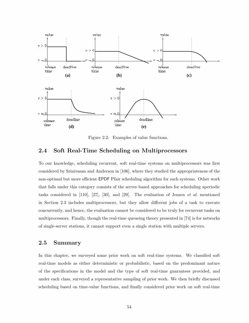
(a) (b) (c)

(d) (e)

ABCDE ABCDE

ABCDE ABCDE ABCDE

FGH

FGH FGH

FGHFGH

FIH FIH FIH

FIH FIH

JECEBKELMNE JECEBKELMNE JECEBKELMNE

JECEBKELMNE JECEBKELMNE

OEBOCMPE OEBOCMPE OEBOCMPE

OEBOCMPE OEBOCMPE

Figure 2.2: Examples of value functions.

2.4 Soft Real-Time Scheduling on Multiprocessors

To our knowledge, scheduling recurrent, soft real-time systems on multiprocessors was first

considered by Srinivasan and Anderson in [106], where they studied the appropriateness of the

non-optimal but more efficient EPDF Pfair scheduling algorithm for such systems. Other work

that falls under this category consists of the server-based approaches for scheduling aperiodic

tasks considered in [110], [27], [30], and [29]. The evaluation of Jensen et al. mentioned

in Section 2.3 includes multiprocessors, but they allow different jobs of a task to execute

concurrently, and hence, the evaluation cannot be considered to be truly for recurrent tasks on

multiprocessors. Finally, though the real-time queueing theory presented in [74] is for networks

of single-server stations, it cannot support even a single station with multiple servers.

2.5 Summary

In this chapter, we surveyed some prior work on soft real-time systems. We classified soft

real-time models as either deterministic or probabilistic, based on the predominant nature

of the specifications in the model and the type of soft real-time guarantees provided, and

under each class, surveyed a representative sampling of prior work. We then briefly discussed

scheduling based on time-value functions, and finally considered prior work on soft real-time

54

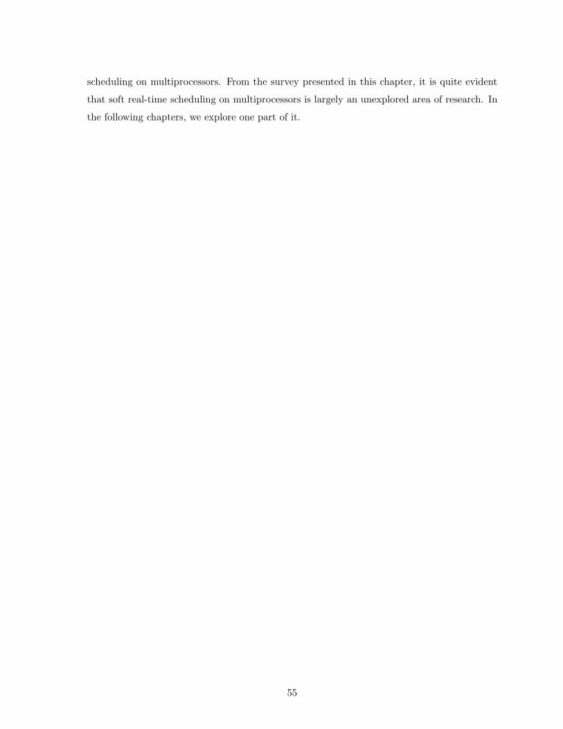
scheduling on multiprocessors. From the survey presented in this chapter, it is quite evident

that soft real-time scheduling on multiprocessors is largely an unexplored area of research. In

the following chapters, we explore one part of it.

55

Chapter 3

Background on Pfair Scheduling

In Chapters 6, 7, and 8, we consider scheduling soft real-time systems using Pfair algorithms.

Before embarking on that endeavor, this chapter describes some basic concepts of Pfair schedul-

ing, provides needed background, and summarizes relevant results from prior work. Since most

prior work on Pfair scheduling has been for hard real-time systems, most of the discussion in

this chapter is with respect to such systems.

The chapter is organized as follows. Section 3.1 motivates the concept of Pfair scheduling.

The basic elements of Pfair scheduling are described in the context of synchronous, periodic

task systems in Section 3.2. Section 3.3 then describes other task models that can be Pfair-

scheduled. Pfair scheduling algorithms are discussed afterwards in Section 3.4, followed by

brief descriptions of some extensions that have been proposed to enhance the practicality of

the Pfair approach. The chapter concludes after summarizing some definitions and results from

prior work that are somewhat technical in nature and that are used in the analyses presented

in later chapters.

3.1 Introduction

In most of the algorithms described so far, jobs are first-class objects in the sense that they

are the basic units of work. Furthermore, timing constraints (e.g., deadlines or tardiness

requirements) are associated with jobs. How job fragments execute is, in general, of little

concern.

This job-oriented paradigm proved sufficient for the optimal online scheduling of periodic

τ (3,7)1

τ (3,7)2

τ (3,7)3

τ (3,7)4

τ (3,7)5

τ (3,7)6

τ (3,7)7

Allocations on Processor 1



L E G E N D

deadline miss

Processors 2 and 3 are idle in [6,7)

0 1 2 3 4 5 6 7 8 9

time

Figure 3.1: A g-EDF schedule with a deadline miss for a task system that is feasible on threeprocessors.

and sporadic real-time task systems on uniprocessors in polynomial time;1 however, it has

so far proved to be inadequate for constructing such schedules on multiprocessors. In what

follows, we will try to illustrate why this is so.

We will begin by considering the example in Figure 3.1. In this example, seven tasks, each

with an execution cost of three time units and a period of seven time units, are scheduled under

g-EDF on three processors.2 A schedule for the first job of each task is shown. Here, the jobs

of τ1, . . . , τ6 complete executing by time six, whereas that of τ7 does not execute at all until

time six and its deadline is at time seven. Though the cumulative processing capacity available

in [6, 7) is sufficient to meet the needs of τ7’s job, restrictions on concurrency prevent it from

using all but one processor, and it misses its deadline at time 7 with two units of computation

pending. It is appropriate to note that, as remarked by Liu in [81], and echoed by Baruah et

al. in [25], “the simple fact that a task can use only one resource even when several of them

are free at the same time adds a surprising amount of difficulty to the scheduling of multiple

resources.”

1The time complexity of an online scheduling algorithm is given by the time required to make a singlescheduling decision.

2Note that the task system in this example cannot be partitioned among three processors, and hence, cannotbe scheduled correctly under any partitioning-based algorithm.

57

τ (3,9)3

τ (5,6)2

τ (5,6)1



missdeadlineis idle

Processor 2

L E G E N D

0 2 4 6 8 10 12 14 16 18

time

Figure 3.2: An LLF schedule with a deadline miss for a task system that is feasible on twoprocessors.

It is clear that τ7’s deadline miss can be averted by appropriately substituting its execution

for those of two of the other tasks, and one may be tempted to attempt using the LLF scheduling

algorithm to fix the problem. Though LLF can avert the deadline miss in the example above,

it is not optimal either. An example of a feasible task system that misses a deadline under

LLF is provided in Figure 3.2. In this example also, there exists a time interval (which is [5, 6))

where a processor is idled due to concurrency restrictions, which in turn leads to the deadline

miss indicated in the figure. Note that idling in this case can be avoided by postponing the

execution of either τ1,1 or τ2,1 by one time unit in exchange for executing τ3,1 earlier. However,

such ad-hoc rules cannot solve this noted problem for any arbitrary task system, and until the

work of Baruah et al., which is described below, it was doubtful whether systematic rules could

be devised at all. In fact, fueled by some negative results, including one by Dertouzos and

Mok in [47], which states that there does not exist an optimal algorithm for scheduling a set of

one-shot, real-time tasks3 on a multiprocessor if not all the release times, execution costs, and

deadlines of all tasks are known a priori , the problem of optimally scheduling periodic and

sporadic tasks online on a multiprocessor was believed to be NP-hard, and the focus seemed

to be on developing efficient heuristics [95, 113].

3A one-shot, real-time task releases a single job. The sole job is associated with a release time, executionrequirement, and a deadline.

58

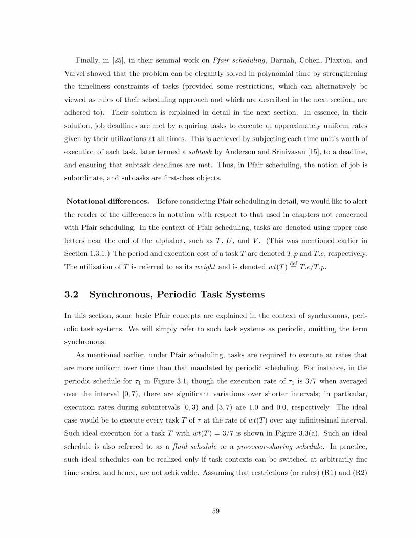
Finally, in [25], in their seminal work on Pfair scheduling , Baruah, Cohen, Plaxton, and

Varvel showed that the problem can be elegantly solved in polynomial time by strengthening

the timeliness constraints of tasks (provided some restrictions, which can alternatively be

viewed as rules of their scheduling approach and which are described in the next section, are

adhered to). Their solution is explained in detail in the next section. In essence, in their

solution, job deadlines are met by requiring tasks to execute at approximately uniform rates

given by their utilizations at all times. This is achieved by subjecting each time unit’s worth of

execution of each task, later termed a subtask by Anderson and Srinivasan [15], to a deadline,

and ensuring that subtask deadlines are met. Thus, in Pfair scheduling, the notion of job is

subordinate, and subtasks are first-class objects.

Notational differences. Before considering Pfair scheduling in detail, we would like to alert

the reader of the differences in notation with respect to that used in chapters not concerned

with Pfair scheduling. In the context of Pfair scheduling, tasks are denoted using upper case

letters near the end of the alphabet, such as T , U , and V . (This was mentioned earlier in

Section 1.3.1.) The period and execution cost of a task T are denoted T.p and T.e, respectively.

The utilization of T is referred to as its weight and is denoted wt(T )def= T.e/T.p.

3.2 Synchronous, Periodic Task Systems

In this section, some basic Pfair concepts are explained in the context of synchronous, peri-

odic task systems. We will simply refer to such task systems as periodic, omitting the term

synchronous.

As mentioned earlier, under Pfair scheduling, tasks are required to execute at rates that

are more uniform over time than that mandated by periodic scheduling. For instance, in the

periodic schedule for τ1 in Figure 3.1, though the execution rate of τ1 is 3/7 when averaged

over the interval [0, 7), there are significant variations over shorter intervals; in particular,

execution rates during subintervals [0, 3) and [3, 7) are 1.0 and 0.0, respectively. The ideal

case would be to execute every task T of τ at the rate of wt(T ) over any infinitesimal interval.

Such ideal execution for a task T with wt(T ) = 3/7 is shown in Figure 3.3(a). Such an ideal

schedule is also referred to as a fluid schedule or a processor-sharing schedule. In practice,

such ideal schedules can be realized only if task contexts can be switched at arbitrarily fine

time scales, and hence, are not achievable. Assuming that restrictions (or rules) (R1) and (R2)

59

below hold, Baruah et al. showed that ideal execution is not necessary for solving the problem

at hand, and an approximation that closely tracks the ideal is sufficient.

(R1) Tasks are allocated processor time in discrete time units or quanta that are

uniform in size and align on all processors.

(R2) The execution cost and period of each task are integer multiples of the quan-

tum size.

Specifically, Baruah et al. showed that when (R1) and (R2) hold, all the job deadlines of a

feasible periodic task system can be met even if at any time t, the absolute deviation in the

total allocation that each task receives up to t, with respect to the ideal schedule, that is,

its absolute lag, is arbitrarily close to one time unit. They formally defined a schedule in

which (3.1) below holds to be a proportionate-fair schedule, or, in short, a Pfair schedule, for

τ , showed that in such a schedule, all of τ ’s job deadlines are met, and presented an online

algorithm for constructing Pfair schedules.

(∀t, T ∈ τ :: −1 < lag(T, t,S) < 1) (3.1)

The formula for lag is given below in (3.3) after notational conventions and the implications

of the above assumptions are set in place.

Unless otherwise specified, (R1) and (R2) above are assumed to hold. System start time is

zero, and for all t ∈ N, where N is the set of natural numbers,4 the real time interval spanning

[t, t + 1), i.e., the real time between time t and time t + 1 that includes t and excludes t + 1, is

referred to as slot t. Unless otherwise specified, in the context of Pfair scheduling, all references

to time are integral. The quantum size equals the slot size, and on each processor, the i + 1st

quantum is allocated in slot i.5 The interval [t1, t2), consists of slots t1, t1 + 1, . . . , t2 − 1. To

ensure that (R1) holds, scheduling decisions are made only at slot boundaries. In each slot,

each task can be scheduled on at most one processor, and on each processor at most one task

can execute. However, a task can be assigned to different processors in different slots. That

is, a task may migrate across processors, but may not execute concurrently.

An ideal or processor-sharing schedule for τ shall be denoted PSτ ; the subscript τ will

be omitted when the task system under consideration is unambiguous. An actual schedule S

4We assume that N includes zero.

5Quantum and slot are often used interchangeably.

60

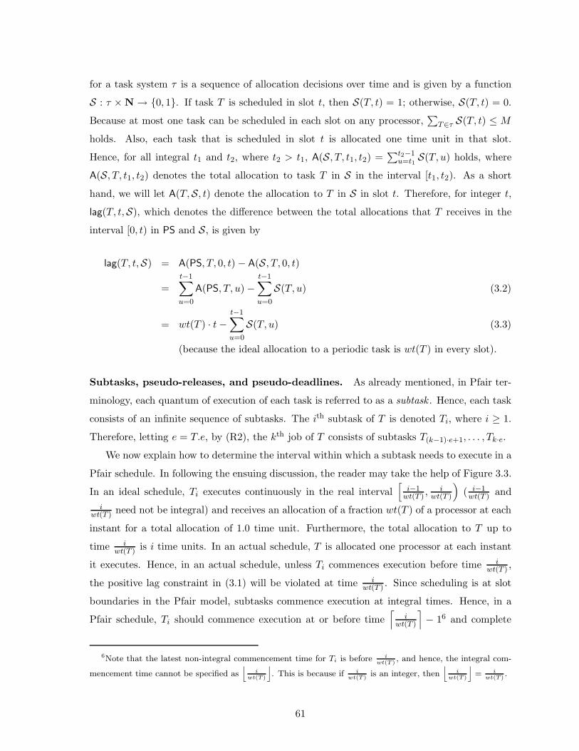
for a task system τ is a sequence of allocation decisions over time and is given by a function

S : τ × N → {0, 1}. If task T is scheduled in slot t, then S(T, t) = 1; otherwise, S(T, t) = 0.

Because at most one task can be scheduled in each slot on any processor,∑

T∈τ S(T, t) ≤ M

holds. Also, each task that is scheduled in slot t is allocated one time unit in that slot.

Hence, for all integral t1 and t2, where t2 > t1, A(S, T, t1, t2) =∑t2−1

u=t1S(T, u) holds, where

A(S, T, t1, t2) denotes the total allocation to task T in S in the interval [t1, t2). As a short

hand, we will let A(T,S, t) denote the allocation to T in S in slot t. Therefore, for integer t,

lag(T, t,S), which denotes the difference between the total allocations that T receives in the

interval [0, t) in PS and S, is given by

lag(T, t,S) = A(PS, T, 0, t) − A(S, T, 0, t)

=

t−1∑

u=0

A(PS, T, u) −t−1∑

u=0

S(T, u) (3.2)

= wt(T ) · t −t−1∑

u=0

S(T, u) (3.3)

(because the ideal allocation to a periodic task is wt(T ) in every slot).

Subtasks, pseudo-releases, and pseudo-deadlines. As already mentioned, in Pfair ter-

minology, each quantum of execution of each task is referred to as a subtask . Hence, each task

consists of an infinite sequence of subtasks. The ith subtask of T is denoted Ti, where i ≥ 1.

Therefore, letting e = T.e, by (R2), the kth job of T consists of subtasks T(k−1)·e+1, . . . , Tk·e.

We now explain how to determine the interval within which a subtask needs to execute in a

Pfair schedule. In following the ensuing discussion, the reader may take the help of Figure 3.3.

In an ideal schedule, Ti executes continuously in the real interval[

i−1wt(T ) ,

iwt(T )

)

( i−1wt(T ) and

iwt(T ) need not be integral) and receives an allocation of a fraction wt(T ) of a processor at each

instant for a total allocation of 1.0 time unit. Furthermore, the total allocation to T up to

time iwt(T ) is i time units. In an actual schedule, T is allocated one processor at each instant

it executes. Hence, in an actual schedule, unless Ti commences execution before time iwt(T ) ,

the positive lag constraint in (3.1) will be violated at time iwt(T ) . Since scheduling is at slot

boundaries in the Pfair model, subtasks commence execution at integral times. Hence, in a

Pfair schedule, Ti should commence execution at or before time⌈

iwt(T )

⌉

− 16 and complete

6Note that the latest non-integral commencement time for Ti is before iwt(T )

, and hence, the integral com-

mencement time cannot be specified as⌊

iwt(T )

⌋

. This is because if iwt(T )

is an integer, then⌊

iwt(T )

⌋

= iwt(T )

.

61

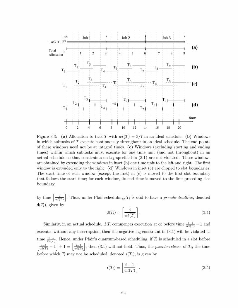
T1

T2T3

T4T5

T6

T7T8

T9

T1

T2T3

T1 T4T5 T7

T6 T8T9

T2

T3

T4

T5T6

T7

T8

T9

0Total Allocation

0 2 4 6 8 10 12 14 16 18 20

1.03/7

3 6 91 2 4 5 7 8

(b)

(d)

(a)Task T

time

(c)

Job 1 Job 2 Job 3

Figure 3.3: (a) Allocation to task T with wt(T ) = 3/7 in an ideal schedule. (b) Windowsin which subtasks of T execute continuously throughout in an ideal schedule. The end pointsof these windows need not be at integral times. (c) Windows (excluding starting and endingtimes) within which subtasks must execute for one time unit (and not throughout) in anactual schedule so that constraints on lag specified in (3.1) are not violated. These windowsare obtained by extending the windows in inset (b) one time unit to the left and right. The firstwindow is extended only to the right. (d) Windows in inset (c) are clipped to slot boundaries.The start time of each window (except the first) in (c) is moved to the first slot boundarythat follows the start time; for each window, its end time is moved to the first preceding slotboundary.

by time⌈

iwt(T )

⌉

. Thus, under Pfair scheduling, Ti is said to have a pseudo-deadline, denoted

d(Ti), given by

d(Ti) =

⌈

i

wt(T )

⌉

. (3.4)

Similarly, in an actual schedule, if Ti commences execution at or before time i−1wt(T ) − 1 and

executes without any interruption, then the negative lag constraint in (3.1) will be violated at

time i−1wt(T ) . Hence, under Pfair’s quantum-based scheduling, if Ti is scheduled in a slot before

⌊

i−1wt(T ) − 1

⌋

+ 1 =⌊

i−1wt(T )

⌋

, then (3.1) will not hold. Thus, the pseudo-release of Ti, the time

before which Ti may not be scheduled, denoted r(Ti), is given by

r(Ti) =

⌊

i − 1

wt(T )

⌋

. (3.5)

62

The steps in determining the pseudo-release times and pseudo-deadlines of subtasks is picto-

rially illustrated in Figure 3.3. The prefix “pseudo,” which is used to indicate that the entity

under consideration is a subtask and not a job, will henceforth be omitted for brevity.

It can easily be shown that all job deadlines of periodic tasks are met in a Pfair schedule.

For this, let S be a Pfair schedule for a periodic task system τ . The deadline of the kth job

of a task T , where k ≥ 1, is given by k · T.p. The total allocation to T up to time k · T.p in

an ideal schedule is k · T.e. By (R2), k · T.p, (k − 1) · T.e, and k · T.e are integers, and recall

that subtasks (k − 1) · T.e + 1, . . . , k · T.e comprise T ’s kth job. Hence, because a subtask can

begin executing only at a slot boundary, subtask k · T.e of T either completes executing by

time k · T.p or does not commence execution until k · T.p. If the former holds, then the kth

job meets its deadline. On the other hand, if the latter holds, then the total allocation to T

at k · T.p is at most k · T.e− 1. Hence, T ’s lag at t is at least one, which, by (3.1), contradicts

the fact that S is Pfair.

PF-windows. The interval [r(Ti), d(Ti)) is referred to as the Pfair-window or PF-window

of Ti and is denoted ω(Ti). The PF-windows of the first few subtasks of a periodic task

with weight 3/7 are shown in Figure 3.4(a). By (3.5) and (3.4), |ω(Ti)| =⌈

iwt(T )

⌉

−⌊

i−1wt(T )

⌋

.

Anderson and Srinivasan have shown the following with respect to the PF-window length of

an arbitrary subtask.

Lemma 3.1 (Anderson and Srinivasan [15]) The length of the PF-window of any subtask

Ti of a task T , |ω(Ti)| = d(Ti) − r(Ti), is either⌈

1wt(T )

⌉

or⌈

1wt(T )

⌉

+ 1.

b-bits. The b-bit or boundary bit is associated with each subtask Ti and is denoted b(Ti).

The b-bit is used by some Pfair scheduling algorithms and indicates the number of slots by

which the PF-windows of Ti and Ti+1 overlap. By (3.4), d(Ti) =⌈

iwt(T )

⌉

holds, and by (3.5),

r(Ti+1) =⌊

iwt(T )

⌋

. Therefore,

b(Ti) =

⌈

i

wt(T )

⌉

−⌊

i

wt(T )

⌋

, (3.6)

and hence, b(Ti) is either zero or one. That is, two consecutive PF-windows are either disjoint

or overlap by at most one slot. As will be discussed later, (3.6) also defines the b-bits of

subtasks in other task models considered under Pfair scheduling.

63

T3

T1

0 1 2 3 4 5 76 8

T3

T2

T1

0 1 2 3 4 5 76 80 1 2 3 4 5 76

T3

T2

T1

0 1 2 3 4 5 76

T1

T2

T3

(a) (b) (c) (d)

Figure 3.4: (a) PF-windows of the first job of a periodic (or sporadic) task T with weight 3/7. Thisjob consists of subtasks T1, T2, and T3, each of which must be scheduled within its window. (Thispattern repeats for every job.) (b) PF-windows of an IS task. Subtask T2 is released one time unitlate. Here, Θ(T1) = 0 while Θ(T2) = Θ(T3) = 1. (c) PF-windows of a GIS task. Subtask T2 is absentand subtask T3 is released one time unit late. (d) PF- and IS-windows of the first job of a GIS taskwith early releases. All the subtasks of this job are eligible when the job arrives. (The deadline-basedpriority definition of the Pfair scheduling algorithms and the prohibition of parallel execution of a taskensure that the subtasks execute in the correct sequence.) For each subtask, its PF-window consists ofthe solid part; the IS-window includes the dashed part, in addition. For example, T2’s PF-window is[2, 5) and its IS-window is [0, 5).

Group deadlines. Like the b-bit, the group deadline is a parameter that is associated with

each subtask and used by some Pfair scheduling algorithms. The group deadline of subtask Ti

is denoted D(Ti). Group deadlines are used for correctly scheduling task systems with one or

more heavy tasks with weights in the range [1/2, 1).

By Lemma 3.1, all the PF-windows of a heavy task with weight less than one are of

length two or three. For such a heavy task, “subtask groups,” which are maximal sequences

of subtasks, satisfying the following two properties with respect to their PF-windows, can be

defined: each window, except possibly of the first subtask in the sequence, is of length two, and

every consecutive pair of windows is overlapping. In Figure 3.5(a), T1, T2 is one such sequence

in which the first window is of length two; T3, . . . , T5 and T6, . . . , T8 are other such sequences

with a 3-window7 as the first window. In each sequence, if any subtask is not scheduled until

its last slot, then all subsequent subtasks will be forced to be scheduled in their last slots as

well, and in that sense constitute a “group.” In addition, if the last subtask in the group is

followed by a subtask with a 3-window, as in the first two groups considered above, then this

subtask will be precluded from being scheduled in its first slot (when any subtask in the group

is scheduled in its last slot). However, no later subtask is directly impacted. Thus, the group

deadline of Ti can be defined as the earliest time t after r(Ti) such that t is the release time

of some subtask and no subtask released at or after t is directly influenced by whether Ti is

scheduled in its last slot.

Informally, for a heavy periodic task with weight less than one, the end of each slot that is

7A window spanning k slots is referred to as a k-window .

64

T2

T1

T3

T4

T5

T7

T8

T6

T1

T2

T3

T4

T5

T7

T6

T8

1 2 3 4 5 60 7 10 1198

(a) (b)

D D D

1 2 3 4 5 60 7 1098

time

12 1311

D D D D

Figure 3.5: Illustration of group deadlines using a task T with weight 8/11. Group deadlinesare marked with a “D.” (a) T is synchronous, periodic. The group deadlines of T1 and T2 areat time 4, and those of T3, . . . , T5 and T6, . . . , T8 are at times 8 and 11, respectively. (b) Tis an IS task and its subtasks T2 and T6 are released late. Nevertheless, the group deadlineof T1 is still at time 4. However, the group deadline of T2 is at time 5. Similarly, thoughT6 is released one time unit late, the group deadlines of T3, . . . , T5 are computed under theassumption that T6 would be released in time, and hence, are at time 9. The group deadlinesof T6, . . . , T8 are at time 13.

not the first slot of the PF-window of any of its subtasks is a group deadline. In Figure 3.5(a),

times 4, 8, and 11 are group deadlines for T in the interval [0, 11]. Note that no subtask is

released at time 3, 7, or 10. Group deadline of subtask Ti can then be defined as D(Ti) =

(min u : u ≥ d(Ti)∧ u is a group deadline of T ). For example, in Figure 3.5(a), D(T1) = 4 and

D(T6) = 11.

Group deadlines of a heavy task T can be computed more directly in constant time by

noting that each group deadline of T corresponds to the pseudo-deadline of some subtask of a

complementary task of T , i.e., a task with weight 1 − wt(T ). Therefore D(Ti) is given by the

earliest time at or after d(Ti) that is a pseudo-deadline of a complementary task of T , and can

be shown to be

⌈⌈

iwt(T )

×(1−wt(T ))⌉

1−wt(T )

⌉

, which can be simplified as follows.8

D(Ti) =

⌈

iwt(T )

⌉

− i

1 − wt(T )

=

⌈

d(Ti) − i

1 − wt(T )

⌉

(3.7)

(3.7) has the nice interpretation that the pseudo-deadline we are interested in is given by that

8The formula derived in [104] is

⌈⌈⌈

i

wt(T )

⌉

×(1−wt(T ))⌉

1−wt(T )

⌉

, which has an extra ceiling that is not needed.

65

of the (d(Ti) − i)th subtask of a complementary task of T .

If T is either light or of weight 1.0, then D(Ti) is defined to be zero.

3.3 Task Model Extensions

In [25], Baruah et al. considered scheduling only synchronous, periodic task systems. Later,

Srinivasan and Anderson extended Pfair scheduling to asynchronous, periodic task systems,

and some other task models, which are described in this section.

The intra-sporadic task model. The intra-sporadic (IS) task model was developed as a

means of supporting sporadic task systems [14, 105], and provides a general notion of recurrent

execution that subsumes that found in the periodic and sporadic task models. Just as the

sporadic model generalizes the periodic model by allowing jobs to be released “late,” the IS

model generalizes the sporadic model by allowing subtasks to be released late, as illustrated

in Figure 3.4(b). More specifically, the separation between r(Ti) and r(Ti+1) is allowed to be

more than⌊

iwt(T )

⌋

−⌊

i−1wt(T )

⌋

, which would be the separation if T were periodic.

The amount of time by which Ti is released late (in comparison to its release time if T were

periodic) is referred to as the offset of Ti and is denoted Θ(Ti). If Ti’s release is postponed,

then its deadline is also postponed by an equal amount. Further, the release of every later

subtask is postponed by at least Θ(Ti), compared to its release when Θ(Ti) = 0. Hence, if

a later subtask Tk’s release is delayed relative to Ti, then Θ(Tk) > Θ(Ti). Therefore, the

following holds.

k > i ⇒ Θ(Tk) ≥ Θ(Ti) (3.8)

Thus, an IS task is obtained by allowing a task’s windows to be shifted right from where they

would appear if the task were periodic. For a sporadic task, all subtasks that belong to the

same job will have equal offsets. By this discussion, and by (3.5) and (3.4), r(Ti) and d(Ti) for

subtask Ti of an IS task are defined as follows.

r(Ti) = Θ(Ti) +

⌊

i − 1

wt(T )

⌋

(3.9)

d(Ti) = Θ(Ti) +

⌈

i

wt(T )

⌉

(3.10)

66

The generalized intra-sporadic task model. Apart from the IS task model, Srinivasan

and Anderson introduced the generalized intra-sporadic (GIS) task model also in [105]. This

model extends the IS task model by allowing subtasks to be omitted or skipped; however, the

spacing between subtasks that are not skipped may not be decreased in comparison to how

they are spaced in a periodic task. Specifically, subtask Ti may be followed by subtask Tk,

where k > i+1 if the following holds: r(Tk)− r(Ti) is at least⌊

k−1wt(T )

⌋

−⌊

i−1wt(T )

⌋

. That is, r(Tk)

is not smaller than what it would have been if Ti+1, Ti+2, . . . ,Tk−1 were present and released

as early as possible. For the special case where Tk is the first subtask released by T , r(Tk)

must be at least⌊

k−1wt(T )

⌋

. Figure 3.4(c) shows an example. In this example, though subtask

T2 is omitted, T3 cannot be released before time 4. If a task T , after executing subtask Ti,

releases subtask Tk, then Tk is called the successor of Ti and Ti is called the predecessor of Tk.

The b-bit and group deadline of a subtask Ti of a GIS or an IS task are computed assuming

that all later subtasks are present and are released as early as possible, that is, under the

assumption that Tj is released and Θ(Tj) = Θ(Ti) holds for all j ≥ i, regardless of how the

subtasks are actually released. Hence, b(Ti) is given by (3.6), even if T is an IS or a GIS task;

D(Ti) is increased by Θ(Ti) and is hence given by

D(Ti) = Θ(Ti) +

⌈

iwt(T )

⌉

− i

1 − wt(T )

. (3.11)

The method for determining group deadlines for an IS task is illustrated in Figure 3.5(b).

The lag of an IS or a GIS task T at t in schedule S is also given by (3.1). Computing

A(S, T, 0, t) is explained towards the end of this section.

The early-release task model. The task models described so far are non-work-conserving

in that, to ensure that the lower bound on lag in (3.1) is met, the second and later subtasks of a

job remain ineligible to be scheduled before their release times, even if they are otherwise ready

and some processor is idle. The early-release (ER) task model was introduced by Anderson and

Srinivasan in [13] as a work-conserving variant to allow subtasks to be scheduled before their

release times. Early releasing can be applied to subtasks in any of the task models considered

so far, and unless otherwise specified, it should be assumed that early releasing is enabled.

However, whether subtasks are actually released early is optional. To facilitate this, in this

model, each subtask Ti has an eligibility time e(Ti) that specifies the first time slot in which

67

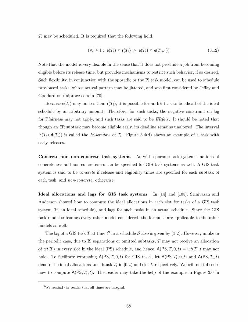
Ti may be scheduled. It is required that the following hold.

(∀i ≥ 1 :: e(Ti) ≤ r(Ti) ∧ e(Ti) ≤ e(Ti+1)) (3.12)

Note that the model is very flexible in the sense that it does not preclude a job from becoming

eligible before its release time, but provides mechanisms to restrict such behavior, if so desired.

Such flexibility, in conjunction with the sporadic or the IS task model, can be used to schedule

rate-based tasks, whose arrival pattern may be jittered, and was first considered by Jeffay and

Goddard on uniprocessors in [70].

Because e(Ti) may be less than r(Ti), it is possible for an ER task to be ahead of the ideal

schedule by an arbitrary amount. Therefore, for such tasks, the negative constraint on lag

for Pfairness may not apply, and such tasks are said to be ERfair . It should be noted that

though an ER subtask may become eligible early, its deadline remains unaltered. The interval

[e(Ti), d(Ti)) is called the IS-window of Ti. Figure 3.4(d) shows an example of a task with

early releases.

Concrete and non-concrete task systems. As with sporadic task systems, notions of

concreteness and non-concreteness can be specified for GIS task systems as well. A GIS task

system is said to be concrete if release and eligibility times are specified for each subtask of

each task, and non-concrete, otherwise.

Ideal allocations and lags for GIS task systems. In [14] and [105], Srinivasan and

Anderson showed how to compute the ideal allocations in each slot for tasks of a GIS task

system (in an ideal schedule), and lags for such tasks in an actual schedule. Since the GIS

task model subsumes every other model considered, the formulas are applicable to the other

models as well.

The lag of a GIS task T at time t9 in a schedule S also is given by (3.2). However, unlike in

the periodic case, due to IS separations or omitted subtasks, T may not receive an allocation

of wt(T ) in every slot in the ideal (PS) schedule, and hence, A(PS, T, 0, t) = wt(T ).t may not

hold. To facilitate expressing A(PS, T, 0, t) for GIS tasks, let A(PS, Ti, 0, t) and A(PS, Ti, t)

denote the ideal allocations to subtask Ti in [0, t) and slot t, respectively. We will next discuss

how to compute A(PS, Ti, t). The reader may take the help of the example in Figure 3.6 in

9We remind the reader that all times are integral.

68

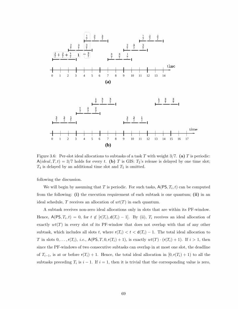
0 1 2 3 4 5 6 7 8 9 10 11 12 13 14

(a)

(b)0 1 2 3 4 5 6 7 8 9 10 11 12 13 14 15 16 17

QRQR QR

QRQR QR

QR QR

QR

QR QR

QR QR SRT T UVWR WR

SR

SR

SR

SRWR

QR

QR

QRQRWR

XYZ[

XYZ[

QR SRWR WR

SR

SR

QR

UQR

Figure 3.6: Per-slot ideal allocations to subtasks of a task T with weight 3/7. (a) T is periodic:A(ideal, T, t) = 3/7 holds for every t. (b) T is GIS: T2’s release is delayed by one time slot;T4 is delayed by an additional time slot and T5 is omitted.

following the discussion.

We will begin by assuming that T is periodic. For such tasks, A(PS, Ti, t) can be computed

from the following: (i) the execution requirement of each subtask is one quantum; (ii) in an

ideal schedule, T receives an allocation of wt(T ) in each quantum.

A subtask receives non-zero ideal allocations only in slots that are within its PF-window.

Hence, A(PS, Ti, t) = 0, for t 6∈ [r(Ti), d(Ti) − 1]. By (ii), Ti receives an ideal allocation of

exactly wt(T ) in every slot of its PF-window that does not overlap with that of any other

subtask, which includes all slots t, where r(Ti) < t < d(Ti) − 1. The total ideal allocation to

T in slots 0, . . . , r(Ti), i.e., A(PS, T, 0, r(Ti) + 1), is exactly wt(T ) · (r(Ti) + 1). If i > 1, then

since the PF-windows of two consecutive subtasks can overlap in at most one slot, the deadline

of Ti−1, is at or before r(Ti) + 1. Hence, the total ideal allocation in [0, r(Ti) + 1) to all the

subtasks preceding Ti is i − 1. If i = 1, then it is trivial that the corresponding value is zero,

69

which is equal to i − 1. It therefore follows that

A(PS, Ti, r(Ti)) = A(PS, T, 0, r(Ti) + 1) − (i − 1) = wt(T ) · (r(Ti) + 1) − (i − 1). (3.13)

For example, in Figure 3.6(a), r(T3) = 4. Hence, wt(T ) · (r(T3) + 1) = (3/7) · 5 = 15/7. Here,

i = 3, and therefore, A(PS, T3, r(T3)) = 15/7 − 2 = 1/7 as marked in the figure.

To compute A(Ti, d(Ti) − 1), we note the following. The total ideal allocation to subtasks

T1, . . . , Ti in [0, d(Ti)) is exactly i quanta. In [0, d(Ti) − 1), T receives a total ideal allocation

of wt(T ) · (d(Ti) − 1), which is due to subtasks T1, . . . , Ti only. Further, no subtask preceding

Ti receives a non-zero allocation in slot d(Ti) − 1. Therefore,

A(PS, Ti, d(Ti) − 1) = i − wt(T ) · (d(Ti) − 1). (3.14)

Referring to the example in Figure 3.6(a) again, d(T2) = 5. Hence, wt(T ) · (d(T2) − 1) =

(3/7) · 4 = 12/7. Here i = 2, and so, A(PS, T2, 4) = 2 − 12/7 = 2/7.

Recall that in an IS task system, each time a subtask release is postponed, the total

postponement in the release of each future subtask is increased by an equal amount. Hence,

the formulas in (3.13) and (3.14) hold for IS tasks also (with the difference that r(Ti) and d(Ti)

on the right-hand side correspond to values obtained using (3.5) and (3.4), respectively, i.e.,

assuming T were periodic, whereas those on the left-hand side correspond to the actual GIS

release time and deadline given by (3.9) and (3.10), respectively). Informally, when a subtask

is shifted, its per-slot allocations simply move with its window. Finally, allocations to subtasks

that are omitted in a GIS task system simply become zero. Per-slot allocations of no other

subtasks are impacted. Substituting values for r(Ti) and d(Ti) from (3.5) and (3.4) in (3.13)

and (3.14) above, A(PS, Ti, t) is given by

A(PS, Ti, u) =

(⌊

i−1wt(T )

⌋

+ 1) × wt(T ) − (i − 1), u = r(Ti)

i − (⌈

iwt(T )

⌉

− 1) × wt(T ), u = d(Ti) − 1

wt(T ), r(Ti) < u < d(Ti) − 1

0, otherwise

(3.15)

As shown in Figure 3.6, A(PS, T, u) usually equals wt(T ), but in certain slots, it may be less

than wt(T ) due to omitted or delayed subtasks. Also, the total allocation that a subtask

Ti receives in the slots that span its window is exactly one in the ideal schedule. These

70

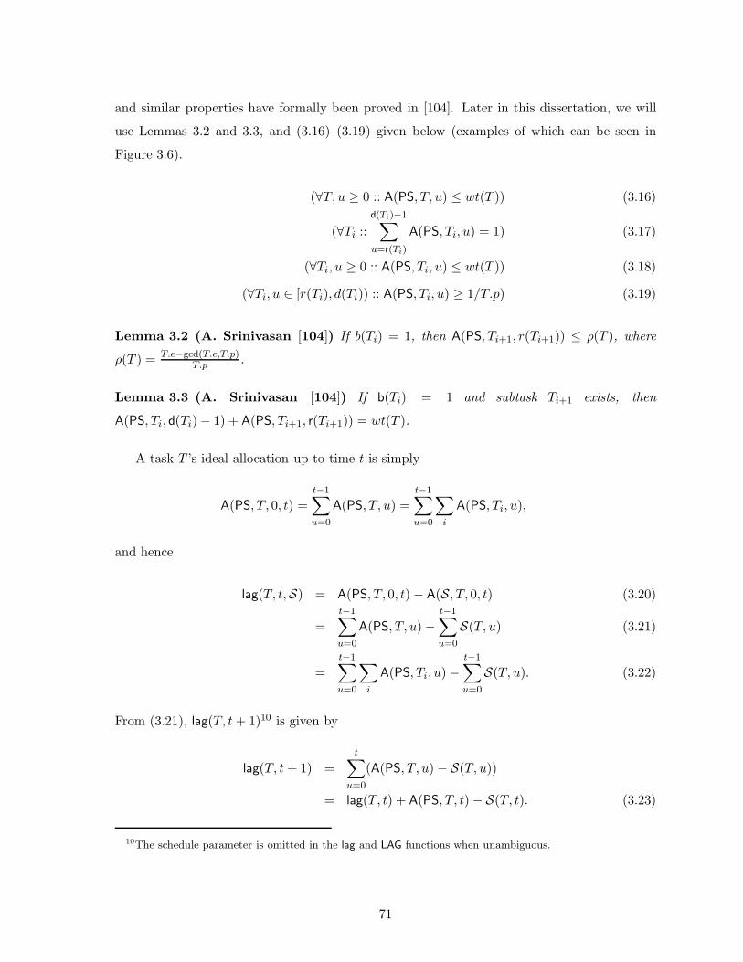
and similar properties have formally been proved in [104]. Later in this dissertation, we will

use Lemmas 3.2 and 3.3, and (3.16)–(3.19) given below (examples of which can be seen in

Figure 3.6).

(∀T, u ≥ 0 :: A(PS, T, u) ≤ wt(T )) (3.16)

(∀Ti ::

d(Ti)−1∑

u=r(Ti)

A(PS, Ti, u) = 1) (3.17)

(∀Ti, u ≥ 0 :: A(PS, Ti, u) ≤ wt(T )) (3.18)

(∀Ti, u ∈ [r(Ti), d(Ti)) :: A(PS, Ti, u) ≥ 1/T.p) (3.19)

Lemma 3.2 (A. Srinivasan [104]) If b(Ti) = 1, then A(PS, Ti+1, r(Ti+1)) ≤ ρ(T ), where

ρ(T ) = T.e−gcd(T.e,T.p)T.p .

Lemma 3.3 (A. Srinivasan [104]) If b(Ti) = 1 and subtask Ti+1 exists, then

A(PS, Ti, d(Ti) − 1) + A(PS, Ti+1, r(Ti+1)) = wt(T ).

A task T ’s ideal allocation up to time t is simply

A(PS, T, 0, t) =t−1∑

u=0

A(PS, T, u) =t−1∑

u=0

∑

i

A(PS, Ti, u),

and hence

lag(T, t,S) = A(PS, T, 0, t) − A(S, T, 0, t) (3.20)

=

t−1∑

u=0

A(PS, T, u) −t−1∑

u=0

S(T, u) (3.21)

=

t−1∑

u=0

∑

i

A(PS, Ti, u) −t−1∑

u=0

S(T, u). (3.22)

From (3.21), lag(T, t + 1)10 is given by

lag(T, t + 1) =

t∑

u=0

(A(PS, T, u) − S(T, u))

= lag(T, t) + A(PS, T, t) − S(T, t). (3.23)

10The schedule parameter is omitted in the lag and LAG functions when unambiguous.

71

Similarly, by (3.21) again, for any 0 ≤ t′ ≤ t,

lag(T, t + 1) = lag(T, t′) +

t∑

u=t′

(A(PS, T, u) − S(T, u))

= lag(T, t′) + A(PS, T, t′, t + 1) − A(S, T, t′, t + 1) (3.24)

≤ lag(T, t′) + (t + 1 − t′) · wt(T ) − A(S, T, t′, t + 1) (by (3.16)). (3.25)

Another useful definition, the total lag for a task system τ in a schedule S at time t, LAG(τ, t,S),

or more concisely, LAG(τ, t), is given by

LAG(τ, t) =∑

T∈τ

lag(T, t). (3.26)

Using (3.23), (3.24), and (3.26), LAG(τ, t + 1) can be expressed as follows. In (3.28) below,

0 ≤ t′ ≤ t holds.

LAG(τ, t + 1) = LAG(τ, t) +∑

T∈τ

(A(PS, T, t) − S(T, t)) (3.27)

LAG(τ, t + 1) = LAG(τ, t′) +t∑

u=t′

∑

T∈τ

(A(PS, T, u) − A(S, T, u))

= LAG(τ, t′) + A(PS, τ, t′, t + 1) − A(S, τ, t′, t + 1) (3.28)

(3.27) and (3.28) above can be rewritten as follows using (3.16).

LAG(τ, t + 1) ≤ LAG(τ, t) +∑

T∈τ (wt(T ) − S(T, t)) (3.29)

LAG(τ, t + 1) ≤ LAG(τ, t′) + (t + 1 − t′) ·∑T∈τ wt(T ) − A(S, τ, t′, t + 1) (3.30)

= LAG(τ, t′) + (t + 1 − t′) ·∑T∈τ wt(T ) −∑tu=t′

∑

T∈τ S(T, u) (3.31)

3.4 Pfair Scheduling Algorithms

A schedule for a GIS task system is valid or correct iff each subtask is scheduled in its IS-

window. In a valid schedule S, lag(T, t,S) < 1 holds for all tasks T at all times t. As mentioned

above, the constraint lag(T, t,S) > −1 of (3.1) may not hold due to early releases. As shown

72

in [25] and [14], a valid schedule exists for a GIS task system τ on M processors iff

∑

T∈τ

wt(T ) ≤ M (3.32)

holds.

Optimal Pfair algorithms. Pfair scheduling algorithms function by choosing at the begin-

ning of each time slot, at most M eligible subtasks for execution in that time slot. The time

complexity of a Pfair scheduling algorithm refers to the worst-case time needed for selecting

any such set of M subtasks. At present, three optimal Pfair scheduling algorithms that can

correctly schedule any feasible GIS task system in polynomial time are known, namely, PF [25],

PD [26], and PD2 [15, 105].11 All the three algorithms are based on a common approach: in

each algorithm, subtask priorities are first determined on an earliest-pseudo-deadline-first ba-

sis; ties are then resolved using tie-breaking rules. The algorithms differ in their choice of

tie-breaking rules. PF, proposed by Baruah et al. in [25], is the earliest, and uses rules that

cannot be applied in constant time, and hence, is not considered efficient. PF was followed

by PD, which was proposed by Baruah, Gehrke, and Plaxton in [26]. Though tie-breaking

under PD requires only constant time, it uses more rules than necessary. In [15], Anderson

and Srinivasan showed that two of PD’s tie-breaking parameters are redundant, and presented

the simpler and more efficient PD2 algorithm. PF and PD were proved optimal for scheduling

only synchronous, periodic task systems. In contrast, Srinivasan and Anderson showed that

PD2 is optimal for scheduling GIS task systems [105]. PD2’s tie-breaking rules subsume those

of PF and PD; hence, it follows that PF and PD are also optimal for GIS task systems. As

PD2 is the most efficient of the three algorithms, we limit ourselves to describing the priority

definition of PD2 here. Readers interested in the other algorithms are referred to their primary

sources.

Algorithm PD2. Apart from pseudo-deadlines of subtasks, PD2 uses their b-bits and group

deadlines in determining the priorities of subtasks. Under PD2, subtask Ti’s priority is at least

that of subtask Uj, denoted Ti � Uj , if one of the following hold.

1. d(Ti) < d(Uj)

11PF and PD stand for Pfair and pseudo-deadline, respectively.

73

0 1 2 3 4 5 6 7 8 9 10 0 1 2 3 4 5 6 7 8 9 100 1 2 3 4 5 6 7 8 9 10

(b)(a) (c)

\] _ \] _ \] _

abcde

fadcghe

iadcghe

jagcdekagcde

ll

ll

ll

ll

ll

ll

ll

ll

ll

l l l l l l l l l l l l l l l

ll l ll l l ll l l l ll l

l ll l

ll

ll

l l

Figure 3.7: A schedule for the first few jobs of tasks T , U , V , W , and Z with weights asspecified under (a) PD2 and (b) EPDF. (c) A schedule for tasks T , U , V , and W under WM.No subtask is early released in any schedule. In each schedule, the slot in which a subtask isscheduled is indicated using an “X.”

2. d(Ti) = d(Uj) and b(Ti) > b(Uj)

3. d(Ti) = d(Uj), b(Ti) = b(Uj) = 1, and D(Ti) ≥ D(Uj).

Any ties that may remain after applying the above rules can be resolved arbitrarily. An

example schedule under PD2 is shown in Figure 3.7(a). The time complexity of PD2 is

O(min(N,M log N)).

Algorithm EPDF. EPDF is a derivative of the optimal algorithms in that it schedules sub-

tasks on an earliest-pseudo-deadline-first basis but avoids using any tie-breaking rule. Under

EPDF, ties among subtasks with equal deadlines is resolved arbitrarily. Anderson and Srini-

vasan have shown that, though not optimal in general, EPDF can correctly schedule all task

systems that are feasible on two processors [15, 106]. An example schedule under EPDF is

shown in Figure 3.7(b). Note the difference in allocations at time 0, in comparison to a sched-

ule under PD2 for the same task set in inset (a). In [106], Srinivasan and Anderson noted that

EPDF may be preferable to the optimal algorithms for soft real-time systems, where bounded

tardiness is tolerable, and for dynamic task systems, where the use of tie-breaking rules may

not be acceptable. They considered its efficacy for scheduling soft real-time systems, and

showed that EPDF can ensure a tardiness of at most q quanta for task systems in which the

74

sum of the weights of the heaviest M − 1 tasks is at most q·M+1q+1 .

Other algorithms. In the algorithms considered above, task priorities are determined at

run-time based on subtask deadlines, and hence, these are dynamic-priority algorithms. More

specifically, since the relative priorities between jobs can differ at different times, these are

unrestricted-dynamic-priority algorithms. For example, in Figure 3.7, all the subtasks of U

and V that are depicted belong to the first jobs of those tasks. At time 0, U ’s job has a higher

priority than V ’s, whereas at time 1, the converse holds.

Algorithms have been proposed for constructing Pfair schedules using static task priorities

also. The motivation for such effort is to enable generating Pfair schedules in systems where

practical factors limit the use of dynamic priorities. In [21], Baruah proposed the weight-

monotonic (WM) scheduling algorithm that prioritizes eligible subtasks on the basis of task

weights and developed a sufficient schedulability test for WM on uniprocessor systems. WM was

later considered by Moir and Ramamurthy for multiprocessor systems in [96], and generalized

by Ramamurthy under the name rational rate-monotonic (RRM) for systems with arbitrary

deadlines [97].

Despite using static priorities for tasks, algorithms like WM cannot be considered static-

priority algorithms in the conventional sense because under Pfair scheduling algorithms, an

otherwise ready task may be ineligible for execution so that the negative constraint on lag in

(3.1) is not violated. Hence, the relative priorities between two tasks, when considered in the

conventional sense, may be different at different times. For example, in the WM schedule in

Figure 3.7(c), T has the highest priority when it has an eligible subtask. Each job of T has an

execution cost of three, and hence, at time 2, the first job of T is still pending. However, at

time 2, T is not scheduled whereas U and V are, and hence, T can be thought of as having a

lower priority than these other tasks. Therefore, results on static-priority scheduling discussed

in Chapter 1 are not applicable to Pfair algorithms that use static task priorities.

3.5 Practical Enhancements

Subsequent to the initial research on Pfair scheduling, which was described in the previous

section, and which is suitable only for independent and static task systems, several mecha-

nisms have been proposed to support real systems wherein tasks may share resources, and

task parameters may change at run-time. Techniques have also been proposed to mitigate

75

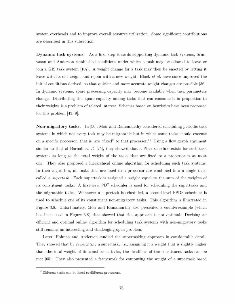
system overheads and to improve overall resource utilization. Some significant contributions

are described in this subsection.

Dynamic task systems. As a first step towards supporting dynamic task systems, Srini-

vasan and Anderson established conditions under which a task may be allowed to leave or

join a GIS task system [107]. A weight change for a task may then be enacted by letting it

leave with its old weight and rejoin with a new weight. Block et al. have since improved the

initial conditions derived, so that quicker and more accurate weight changes are possible [36].

In dynamic systems, spare processing capacity may become available when task parameters

change. Distributing this spare capacity among tasks that can consume it in proportion to

their weights is a problem of related interest. Schemes based on heuristics have been proposed

for this problem [43, 9].

Non-migratory tasks. In [90], Moir and Ramamurthy considered scheduling periodic task

systems in which not every task may be migratable but in which some tasks should execute

on a specific processor, that is, are “fixed” to that processor.12 Using a flow graph argument

similar to that of Baruah et al. [25], they showed that a Pfair schedule exists for such task

systems as long as the total weight of the tasks that are fixed to a processor is at most

one. They also proposed a hierarchical online algorithm for scheduling such task systems.

In their algorithm, all tasks that are fixed to a processor are combined into a single task,

called a supertask . Each supertask is assigned a weight equal to the sum of the weights of

its constituent tasks. A first-level PD2 scheduler is used for scheduling the supertasks and

the migratable tasks. Whenever a supertask is scheduled, a second-level EPDF scheduler is

used to schedule one of its constituent non-migratory tasks. This algorithm is illustrated in

Figure 3.8. Unfortunately, Moir and Ramamurthy also presented a counterexample (which

has been used in Figure 3.8) that showed that this approach is not optimal. Devising an

efficient and optimal online algorithm for scheduling task systems with non-migratory tasks

still remains an interesting and challenging open problem.

Later, Holman and Anderson studied the supertasking approach in considerable detail.

They showed that by reweighting a supertask, i.e., assigning it a weight that is slightly higher

than the total weight of its constituent tasks, the deadlines of the constituent tasks can be

met [65]. They also presented a framework for computing the weight of a supertask based

12Different tasks can be fixed to different processors.

76

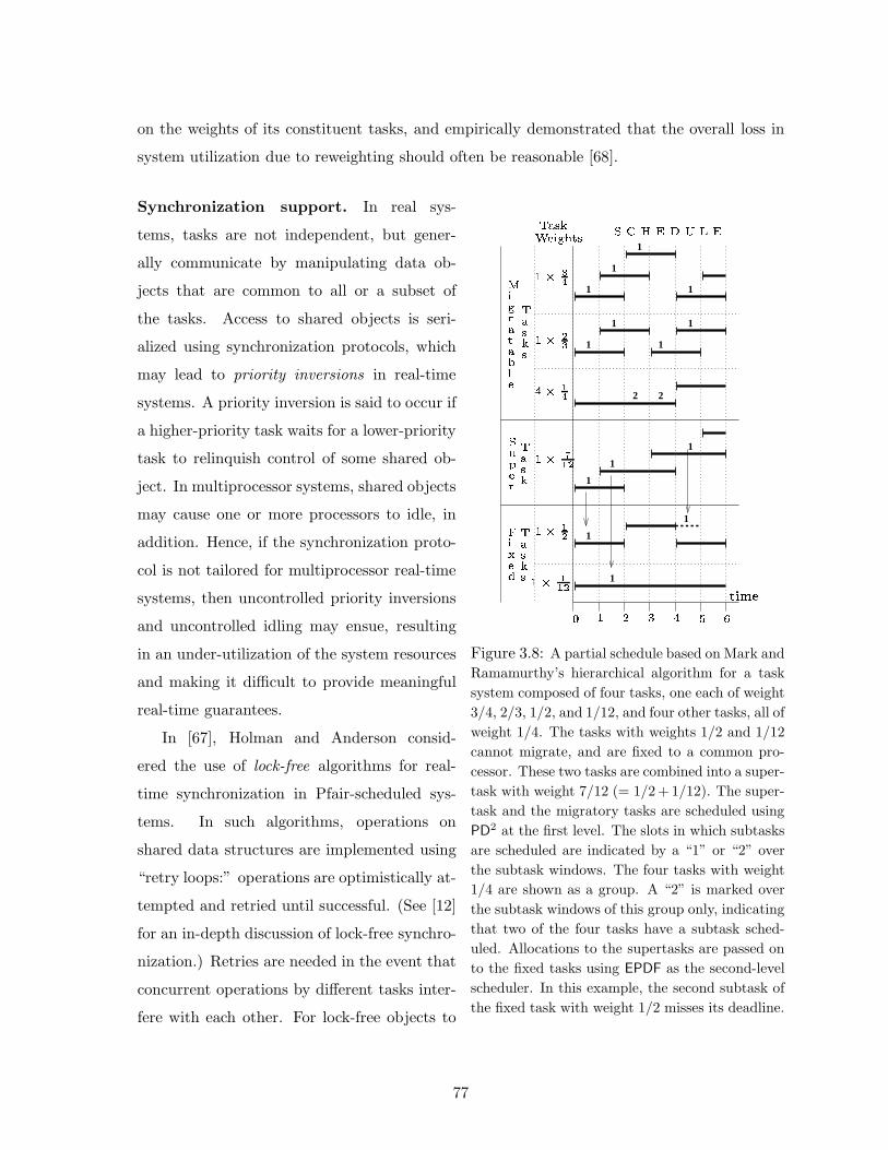
on the weights of its constituent tasks, and empirically demonstrated that the overall loss in

system utilization due to reweighting should often be reasonable [68].

1

1

1

1

1

1

1

2 2

1

1

1

1

1

1

1

mnopqrqstu

vqwxw

vqwx

vqwxw

ynzu{

|}~up

� ��

| � � � � � � �

� � � � � � �

� � ��

� � ��

� � ��

� � ��

� uno�r wvq wx

Figure 3.8: A partial schedule based on Mark and

Ramamurthy’s hierarchical algorithm for a task

system composed of four tasks, one each of weight

3/4, 2/3, 1/2, and 1/12, and four other tasks, all of

weight 1/4. The tasks with weights 1/2 and 1/12

cannot migrate, and are fixed to a common pro-

cessor. These two tasks are combined into a super-

task with weight 7/12 (= 1/2 + 1/12). The super-

task and the migratory tasks are scheduled using

PD2 at the first level. The slots in which subtasks

are scheduled are indicated by a “1” or “2” over

the subtask windows. The four tasks with weight

1/4 are shown as a group. A “2” is marked over

the subtask windows of this group only, indicating

that two of the four tasks have a subtask sched-

uled. Allocations to the supertasks are passed on

to the fixed tasks using EPDF as the second-level

scheduler. In this example, the second subtask of

the fixed task with weight 1/2 misses its deadline.

Synchronization support. In real sys-

tems, tasks are not independent, but gener-

ally communicate by manipulating data ob-

jects that are common to all or a subset of

the tasks. Access to shared objects is seri-

alized using synchronization protocols, which

may lead to priority inversions in real-time

systems. A priority inversion is said to occur if

a higher-priority task waits for a lower-priority

task to relinquish control of some shared ob-

ject. In multiprocessor systems, shared objects

may cause one or more processors to idle, in

addition. Hence, if the synchronization proto-

col is not tailored for multiprocessor real-time

systems, then uncontrolled priority inversions

and uncontrolled idling may ensue, resulting

in an under-utilization of the system resources

and making it difficult to provide meaningful

real-time guarantees.

In [67], Holman and Anderson consid-

ered the use of lock-free algorithms for real-

time synchronization in Pfair-scheduled sys-

tems. In such algorithms, operations on

shared data structures are implemented using

“retry loops:” operations are optimistically at-

tempted and retried until successful. (See [12]

for an in-depth discussion of lock-free synchro-

nization.) Retries are needed in the event that

concurrent operations by different tasks inter-

fere with each other. For lock-free objects to

77

be usable in real-time systems, it is important that bounds on interferences (and hence, retries)

be determined.

While the viability of the lock-free approach for uniprocessor -based real-time systems is

well-known [12], on multiprocessors, lock-free sharing is often considered impractical, because

of difficulties in computing reasonable retry bounds. Nevertheless, Holman and Anderson

argued and showed that for simple objects, such as queues, stacks, and linked lists, quantum-

based scheduling of Pfair algorithms can be exploited to mitigate the overhead considerably.

They also proposed combining tasks accessing common objects into a supertask to further

reduce overhead.

Holman and Anderson also presented locking synchronization protocols under Pfair algo-

rithms for synchronizing accesses to complex objects, and for use in other scenarios where

lock-free approaches may not be suitable [66].

Reducing context-switching costs. In [120], Zhu et al. proposed the boundary fair (BF)

scheduling algorithm for periodic task systems. This algorithm includes heuristics to reduce

the number of scheduler invocations, and thereby, the number of context switches. BF differs

from Pfair algorithms in that it makes scheduling decisions only at time instants that are

multiples of some task period, called boundary time points. At each boundary point tb, up to

k · M subtasks are selected for execution in the interval [tb, tb + k), where tb + k is the next

boundary point. A schedule that reduces the number of context switches is then laid out for

the selected subtasks.

The next section presents some additional technical definitions and results from prior work

that will be used in later chapters.

3.6 Technical Definitions

Active tasks. If subtasks are absent or are released late, then it is possible for a GIS (or IS)

task to have no eligible subtasks and an allocation of zero during certain time slots. Tasks with

and without subtasks in the interval [t, t + `) are distinguished using the following definition

of an active task.

Definition 3.1: A GIS task U is active in slot t if it has one or more subtasks Uj such that

e(Uj) ≤ t < d(Uj). (A task that is active in t is not necessarily scheduled in that slot.)

78

Holes. If fewer than M tasks are scheduled at time t in S, then one or more processors

would be idle in slot t. For each slot, each processor that is idle in that slot is referred to as

a hole. Hence, if k processors are idle in slot t, then there are said to be k holes in t. The

following lemma is a generalization of one proved in [105], and relates an increase in the total

lag of τ , LAG, to the presence of holes.

Lemma 3.4 (Srinivasan and Anderson [105]) If LAG(τ, t + `,S) > LAG(τ, t,S), where

` ≥ 1, then there is at least one hole in the interval [t, t + `).

Intuitively, if there is no idle processor in slots t, . . . , t + ` − 1, then the total allocation in Sin each of those slots to tasks in τ is equal to M . This is at least the total allocation that τ

receives in any slot in the ideal schedule. Therefore, LAG cannot increase.

Task classification(from [105]). Tasks in τ may be classified as follows with respect to a

schedule S and time interval [t, t + `).13

A(t, t + `): Set of all tasks that are scheduled in one or more slots in [t, t + `).

B(t, t + `): Set of all tasks that are not scheduled in any slot in [t, t + `), but are active in one

or more slots in the interval.

I(t, t + `): Set of all tasks that are neither active nor scheduled in any slot in [t, t + `).

As a shorthand, the notation A(t), B(t), and I(t) is used when ` = 1. A(t, t + `), B(t, t + `),

and I(t, t + `) form a partition of τ , i.e., the following holds.

A(t, t + `) ∪ B(t, t + `) ∪ I(t, t + `) = τ ∧A(t, t + `) ∩ B(t, t + `) = B(t, t + `) ∩ I(t, t + `) = I(t, t + `) ∩ A(t, t + `) = ∅

(3.33)

This classification of tasks is illustrated in Figure 3.9(a) for ` = 1. Using (3.26) and (3.33)

above, we have the following.

LAG(τ, t + 1) =∑

T∈A(t)

lag(T, t + 1) +∑

T∈B(t)

lag(T, t + 1) +∑

T∈I(t)

lag(T, t + 1) (3.34)

The next definition identifies the last-released subtask at t of any task U .

13For brevity, we let the task system τ and schedule S be implicit in these definitions.

79

X

X

X

X

X X

��

��

��

�

¡¢£

¤¥¢£

¦§ �©ª

¡

¤¥¦«

(a)

X

X

X

X

X

X

¬ ¬® ¬¯ ¬° ¬±²³ µ

¶· ³ ¹µ º»µ¼¶·

½¾

¶·¿À

ÁÂÃÄ

½¾¿À

(b)

Figure 3.9: (a) Illustration of task classification at time t. IS-windows of two consecutivesubtasks of three GIS tasks T , U , and V are depicted. The slot in which each subtask isscheduled is indicated by an “X.” Because subtask Ti+1 is scheduled at t, T ∈ A(t). No subtaskof U is scheduled at t; however, because the IS-window of Uk overlaps slot t, U is active at t,and hence, U ∈ B(t). Task V is neither scheduled at t, nor is it active at t; therefore, V ∈ I(t).(b) Illustration of displacements. If Ui, scheduled at time t, is removed from the task system,then some subtask that is eligible at t, but scheduled later, can be scheduled at t. In thisexample, it is subtask Vk (scheduled at t + 3). This displacement of Vk results in two moredisplacements, those of Vk+1 and Ui+1, as shown. Thus, there are three displacements in all:∆1 = (Ui, t, Vk, t + 3),∆2 = (Vk, t + 3, Vk+1, t + 4), and ∆3 = (Vk+1, t + 4, Ui+1, t + 5).

Definition 3.2: Subtask Uj is the critical subtask of U at t iff e(Uj) ≤ t < d(Uj) holds, and

no other subtask Uk of U , where k > j, satisfies e(Uk) ≤ t < d(Uk).

For example, in Figure 3.9(a), T ’s critical subtask at both t − 1 and t is Ti+1, and U ’s

critical subtask at t + 1 is Uk+1.

Displacements. To facilitate reasoning about Pfair algorithms, Srinivasan and Anderson

formally defined displacements in [105]. Let τ be a GIS task system and let S be an EPDF

schedule for τ . Then, removing a subtask, say Ti, from τ results in another GIS task system τ ′.

Suppose that Ti is scheduled at t in S. Then, Ti’s removal can cause another subtask, say Uj ,

scheduled after t to shift left to t, which in turn can lead to other shifts, resulting in an EPDF

schedule S ′ for τ ′. Each shift that results due to a subtask removal is called a displacement and

is denoted by a four-tuple 〈X(1), t1,X(2), t2〉, where X(1) and X(2) represent subtasks. This is

equivalent to saying that subtask X(2) originally scheduled at t2 in S displaces subtask X(1)

scheduled at t1 in S. A displacement 〈X(1), t1,X(2), t2〉 is valid iff e(X(2)) ≤ t1. Because there

80

can be a cascade of shifts, there may be a chain of displacements. Such a chain is represented

by a sequence of four-tuples. An example is given in Figure 3.9(b).

The next two lemmas regarding displacements are proved in [105] and [104]. The first

lemma states that in an EPDF schedule, a subtask removal can cause other subtasks to shift

only to their left. According to the second lemma, if a subtask displaces to a slot with a hole,

then its predecessor is scheduled in that slot prior to the displacement.

Lemma 3.5 (from [104]) Let X(1) be a subtask that is removed from τ , and let the re-

sulting chain of displacements in an EPDF schedule for τ be C = ∆1,∆2, . . . ,∆k, where

∆i = 〈X(i), ti,X(i+1), ti+1〉. Then ti+1 > ti for all i ∈ [1, k].

Lemma 3.6 (from [105]) Let ∆ = 〈X(i), ti,X(i+1), ti+1〉 be a valid displacement in any EPDF

schedule. If ti < ti+1 holds and there is a hole in slot ti in that schedule, then X(i+1) is the

successor of X(i).

3.7 Summary

In this chapter, we first motivated the concept of Pfair scheduling and described the Pfair

scheduling of synchronous, periodic tasks. We then considered some other more flexible re-

current task models that can be Pfair scheduled. Later, we discussed some Pfair scheduling

algorithms, and described some techniques that have been proposed to enhance the practical-

ity of Pfair scheduling. Finally, we summarized some technical definitions and results from

prior work that will be used in the analyses presented in Chapters 6 and 7. In these chapters,

we consider the non-optimal EPDF scheduling algorithm in detail, and present some new re-

sults concerning this algorithm. As noted in this chapter, EPDF may be preferable to optimal

algorithms for scheduling soft or dynamic real-time systems.

81

Chapter 4

Tardiness Bounds under Preemptive and

Non-Preemptive Global EDF1

In this chapter, we derive tardiness bounds that can be guaranteed under preemptive and

non-preemptive global EDF (g-EDF and g-NP-EDF) for sporadic real-time task systems on

multiprocessors. In general, overheads due to task preemptions and migrations are lower

under EDF than under the known optimal algorithms. Further, since EDF does not require

the restrictions, which were discussed in Section 1.6, imposed by optimal algorithms, EDF may

be preferable to the optimal algorithms in some settings. However, the worst-case schedulable

utilizations of g-EDF and g-NP-EDF can be quite low, and hence, using their existing validation

tests, which are designed to ensure that no deadline is missed, can be overkill for scheduling

soft real-time systems. The tardiness bounds that we determine in this chapter can instead be

used for validating such systems. As will be seen, no restriction on total system utilization,

except that it not exceed the available processing capacity, is necessary to ensure bounded

tardiness under g-EDF and g-NP-EDF. Hence, effective utilization on multiprocessors can be

improved by using these results while scheduling soft real-time systems.

Instead of deriving tardiness bounds independently for g-EDF and g-NP-EDF, we consider

a more general task model, in which tasks may consist of both preemptive and non-preemptive

segments, and a mixed mode EDF scheduler that allows/restricts preemptions based on the

nature of the task segment under execution. Such a mixed-mode model may be useful for

1Contents of this chapter previously appeared in preliminary form in the following paper:[51] U. Devi and J. Anderson. Tardiness bounds under global EDF scheduling on a multiprocessor. InProceedings of the 26th IEEE Real-Time Systems Symposium, pages 330–341, December 2005.

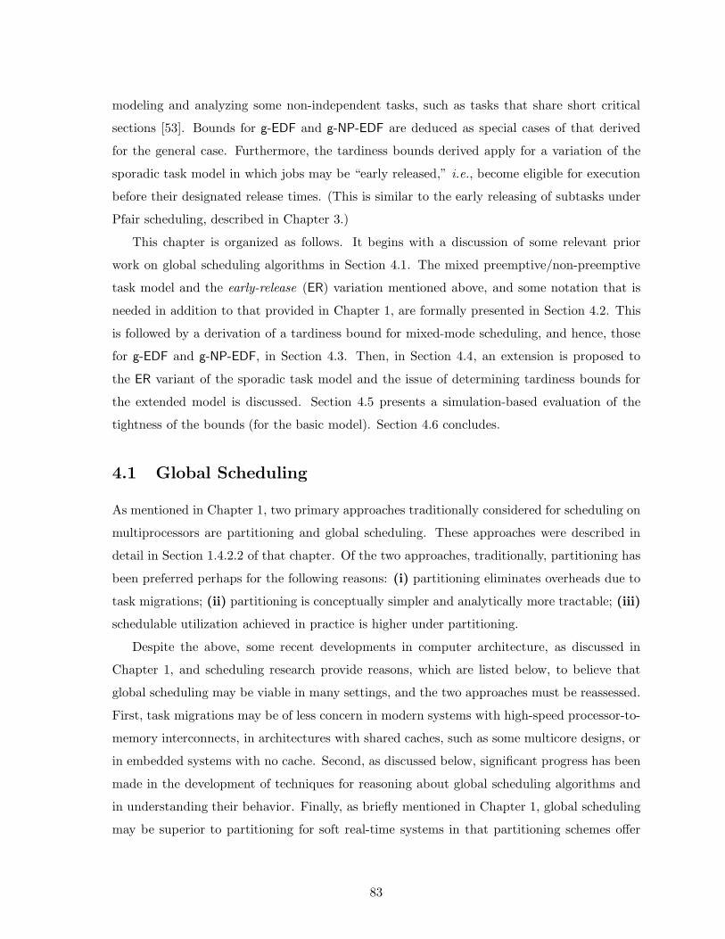
modeling and analyzing some non-independent tasks, such as tasks that share short critical

sections [53]. Bounds for g-EDF and g-NP-EDF are deduced as special cases of that derived

for the general case. Furthermore, the tardiness bounds derived apply for a variation of the

sporadic task model in which jobs may be “early released,” i.e., become eligible for execution

before their designated release times. (This is similar to the early releasing of subtasks under

Pfair scheduling, described in Chapter 3.)

This chapter is organized as follows. It begins with a discussion of some relevant prior

work on global scheduling algorithms in Section 4.1. The mixed preemptive/non-preemptive

task model and the early-release (ER) variation mentioned above, and some notation that is

needed in addition to that provided in Chapter 1, are formally presented in Section 4.2. This

is followed by a derivation of a tardiness bound for mixed-mode scheduling, and hence, those

for g-EDF and g-NP-EDF, in Section 4.3. Then, in Section 4.4, an extension is proposed to

the ER variant of the sporadic task model and the issue of determining tardiness bounds for

the extended model is discussed. Section 4.5 presents a simulation-based evaluation of the

tightness of the bounds (for the basic model). Section 4.6 concludes.

4.1 Global Scheduling

As mentioned in Chapter 1, two primary approaches traditionally considered for scheduling on

multiprocessors are partitioning and global scheduling. These approaches were described in

detail in Section 1.4.2.2 of that chapter. Of the two approaches, traditionally, partitioning has

been preferred perhaps for the following reasons: (i) partitioning eliminates overheads due to

task migrations; (ii) partitioning is conceptually simpler and analytically more tractable; (iii)

schedulable utilization achieved in practice is higher under partitioning.

Despite the above, some recent developments in computer architecture, as discussed in

Chapter 1, and scheduling research provide reasons, which are listed below, to believe that

global scheduling may be viable in many settings, and the two approaches must be reassessed.

First, task migrations may be of less concern in modern systems with high-speed processor-to-

memory interconnects, in architectures with shared caches, such as some multicore designs, or

in embedded systems with no cache. Second, as discussed below, significant progress has been

made in the development of techniques for reasoning about global scheduling algorithms and

in understanding their behavior. Finally, as briefly mentioned in Chapter 1, global scheduling

may be superior to partitioning for soft real-time systems in that partitioning schemes offer

83

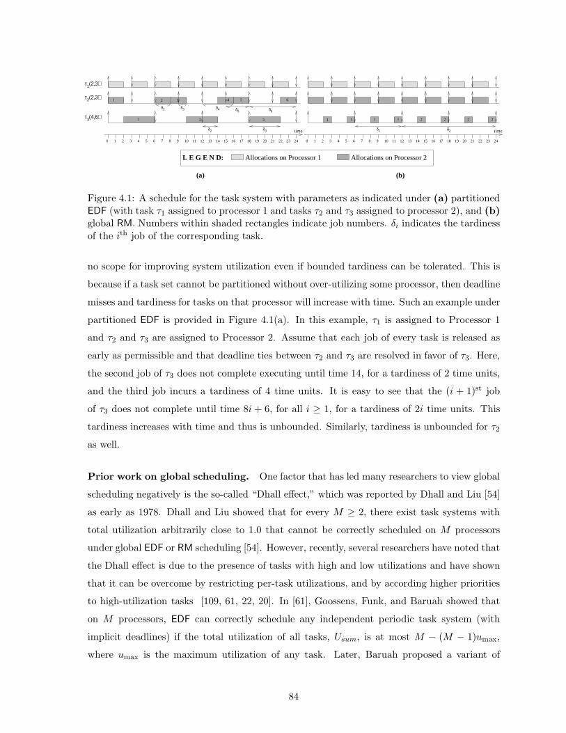
τ (2,3)1

τ (2,3)2

τ (4,6)3

δ3δ2 δ4 δ5 δ6

δ2 δ3 δ1 δ2

(a) (b)

Allocations on Processor 2Allocations on Processor 1L E G E N D:

1 2 3 4 5 6

1 2 3

0 2 3 4 8 9 10 11 12 13 14 15 16 17 18 19 20 21 22 23 241 5 6 7 0 2 3 4 8 9 10 11 12 13 14 15 16 17 18 19 20 21 22 23 241 5 6 7

time time

1 1 1 1 2 2 2 2

Figure 4.1: A schedule for the task system with parameters as indicated under (a) partitionedEDF (with task τ1 assigned to processor 1 and tasks τ2 and τ3 assigned to processor 2), and (b)global RM. Numbers within shaded rectangles indicate job numbers. δi indicates the tardinessof the ith job of the corresponding task.

no scope for improving system utilization even if bounded tardiness can be tolerated. This is

because if a task set cannot be partitioned without over-utilizing some processor, then deadline

misses and tardiness for tasks on that processor will increase with time. Such an example under

partitioned EDF is provided in Figure 4.1(a). In this example, τ1 is assigned to Processor 1

and τ2 and τ3 are assigned to Processor 2. Assume that each job of every task is released as

early as permissible and that deadline ties between τ2 and τ3 are resolved in favor of τ3. Here,

the second job of τ3 does not complete executing until time 14, for a tardiness of 2 time units,

and the third job incurs a tardiness of 4 time units. It is easy to see that the (i + 1)st job

of τ3 does not complete until time 8i + 6, for all i ≥ 1, for a tardiness of 2i time units. This

tardiness increases with time and thus is unbounded. Similarly, tardiness is unbounded for τ2

as well.

Prior work on global scheduling. One factor that has led many researchers to view global

scheduling negatively is the so-called “Dhall effect,” which was reported by Dhall and Liu [54]

as early as 1978. Dhall and Liu showed that for every M ≥ 2, there exist task systems with

total utilization arbitrarily close to 1.0 that cannot be correctly scheduled on M processors

under global EDF or RM scheduling [54]. However, recently, several researchers have noted that

the Dhall effect is due to the presence of tasks with high and low utilizations and have shown

that it can be overcome by restricting per-task utilizations, and by according higher priorities

to high-utilization tasks [109, 61, 22, 20]. In [61], Goossens, Funk, and Baruah showed that

on M processors, EDF can correctly schedule any independent periodic task system (with

implicit deadlines) if the total utilization of all tasks, Usum, is at most M − (M − 1)umax,

where umax is the maximum utilization of any task. Later, Baruah proposed a variant of

84

EDF that prioritizes tasks with utilization exceeding 1/2 over the rest, and showed that the

modified algorithm can correctly schedule any task system with total utilization not exceeding

(M +1)/2. Schedulability tests that can be applied to task systems in which relative deadlines

of tasks can be less than their periods (i.e., constrained-deadline systems) have been developed

by Baker [20] and by Bertogna et al. [33].

The proposed schedulability tests for implicit-deadline systems that depend on umax have

the property that, the total utilization of a task system that is schedulable increases as umax

is decreased. Nevertheless, even with umax = 0.5, half the total available processing capacity

will have to be wasted, if every deadline must be met. This may be overkill for soft real-time

systems that can tolerate bounded deadline misses.

The research discussed above is for preemptive global EDF, or g-EDF. To our knowledge,

non-preemptive global EDF (g-NP-EDF) has been considered only in [23], where a sufficient

schedulability condition is derived for task systems in which the maximum execution cost of

any task is less than the minimum period of any task.

Non-trivial schedulability tests have been developed for global RM scheduling also [16, 20,

34]. However, the schedulable utilizations that these tests allow are less than that allowed

by g-EDF. Furthermore, like partitioning algorithms, global RM (or any global static-priority

algorithm) may not be suitable for soft real-time systems. This is because, task systems exist

in which tardiness for low-priority tasks increases with time when scheduled under RM. Refer

to Figure 4.1(b) for an example. In this example, the ith job of τ3 does not complete until

time 12i, for all i, for a tardiness of 6i time units.

With the above overview of the state-of-the-art in global scheduling, we turn to deriving

tardiness bounds for global EDF. We begin by presenting the additional elements of the task

model used in this chapter.

4.2 Task Model and Notation

The basic task model is the sporadic task model described in Section 1.3.1, augmented for soft

real-time systems as described in Section 1.5. In this section, we describe two generalizations

of the basic task model that we consider in this chapter and also present some additional

notation.

We would like to remind the reader that N denotes the number of tasks in the task system

85

τ under consideration, and M , the number of processors. The total utilization of all the tasks

in τ , Usum(τ), is assumed to not exceed M .

Non-preemptive sections. To provide a common analytic framework for g-EDF and g-

NP-EDF, we consider a more general model than the sporadic task model wherein each job of

each task τi may consist of one or more preemptive and non-preemptive code segments. The

maximum execution cost of any non-preemptive segment of τi is denoted bi and the maximum

value taken over all tasks in τ is denoted bmax(τ). In this extended model, task τi is denoted

using a triple (ei, pi, bi).

Mixed preemptive/non-preemptive scheduling. We will refer to the EDF algorithm

that is cognizant of the non-preemptive segments of a task and executes them non-preemptively

as EDF-P-NP. (In a real implementation, special system calls would be used to inform the

scheduler when a non-preemptive segment is entered and exited.) At any time, higher priority

is accorded to jobs with earlier absolute deadlines, subject to not preempting a job that is

executing in a non-preemptive segment. Ties are resolved arbitrarily but consistently in that

ties between two jobs are resolved identically at all times. A job executing in a preemptive

segment may be preempted by an arriving higher-priority job and may later resume execution

on the same or a different processor. EDF-P-NP reduces to g-EDF when bmax = 0 and to

g-NP-EDF when bi = ei, for all i.

Early releasing. In the model considered in this chapter, jobs of sporadic tasks may be

executed “early,” i.e., before their release times (as stipulated by the sporadic task model),

provided that prior jobs of the same task have completed execution. This is just an application

of the concept described in the context of Pfair scheduling of subtasks in Chapter 3 to task

systems in which jobs are first-class objects. As mentioned in Chapter 3, the flexibility offered

by early releasing can be used for scheduling rate-based tasks [70].

A job that may be executed before its release time is said to be early released . Each job

τi,j is associated with an eligibility time, denoted ì,j, where ì,j ≤ ri,j and ì,j+1 ≥ ì,j for

all i and j. ì,j is the earliest time that τi,j can commence execution. Early releasing does

not alter job deadlines, and hence, how job priorities are determined, but only the set of jobs

that can contend at a given time. When early releasing is enabled, for a concrete task system,

apart from the release time and actual execution cost, the eligibility time of each job is also

specified.

86

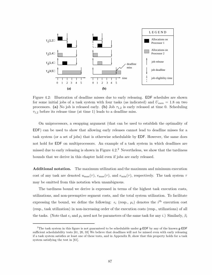
τ1(1,2)

τ2(1,4)

τ3(1,4)

τ4(4,5)

(a) (b)

0 1 2 3 4 5 0 1 2 3 4 5

time

deadline miss

Processor 1

Allocations on

job release

job deadline

job eligibility time

Allocations on

L E G E N D

Processor 2

Figure 4.2: Illustration of deadline misses due to early releasing. EDF schedules are shownfor some initial jobs of a task system with four tasks (as indicated) and Usum = 1.8 on twoprocessors. (a) No job is released early. (b) Job τ1,2 is early released at time 0. Schedulingτ1,2 before its release time (at time 1) leads to a deadline miss.

On uniprocessors, a swapping argument (that can be used to establish the optimality of

EDF) can be used to show that allowing early releases cannot lead to deadline misses for a

task system (or a set of jobs) that is otherwise schedulable by EDF. However, the same does

not hold for EDF on multiprocessors. An example of a task system in which deadlines are

missed due to early releasing is shown in Figure 4.2.2 Nevertheless, we show that the tardiness

bounds that we derive in this chapter hold even if jobs are early released.

Additional notation. The maximum utilization and the maximum and minimum execution

cost of any task are denoted umax(τ), emax(τ), and emin(τ), respectively. The task system τ

may be omitted from this notation when unambiguous.

The tardiness bound we derive is expressed in terms of the highest task execution costs,

utilizations, and non-preemptive segment costs, and the total system utilization. To facilitate

expressing the bound, we define the following: εi (resp., µi) denotes the ith execution cost

(resp., task utilization) in non-increasing order of the execution costs (resp., utilizations) of all

the tasks. (Note that εi and µi need not be parameters of the same task for any i.) Similarly, βi

2The task system in this figure is not guaranteed to be schedulable under g-EDF by any of the known g-EDF

sufficient schedulability tests [61, 20, 33] We believe that deadlines will not be missed even with early releasingif a task system satisfies at least one of these tests, and in Appendix B, show that this property holds for a tasksystem satisfying the test in [61].

87

denotes the ith largest non-preemptive segment cost. For simplicity, we assume the following.

(∀i, j ≤ N :: ei ≤ ej ⇔ bi ≤ bj) (4.1)

The above assumption can easily be seen to hold for both g-EDF and g-NP-EDF. It can be

eliminated for mixed-mode tasks at the expense of either a slightly higher tardiness bound or a

more complicated algorithm (as opposed to a closed-form expression) for choosing tasks whose

execution costs are to be used in computing a less-pessimistic bound. One such algorithm is

described in Section A.3 of Appendix A.

We define the following subsets of tasks in order to lower the pessimism in the bounds

specified. In these definitions, k ≤ N and k2 ≤ k1 ≤ N hold. (These definitions may be

skipped on first reading without loss of continuity and referred back to when needed.) The

purpose of defining these sets is follows. The tardiness bounds derived are dependent upon

the sum of the execution costs of tasks in some subset of all the tasks and that of the non-

preemptive segment costs of tasks in another disjoint subset. While it is simpler to use the

maximum execution costs and maximum non-preemptive segment costs as upper bounds, that

approach overlooks the fact that the subsets are disjoint, and hence, that at most one of the

execution cost and non-preemptive segment cost of a task may be used. The challenge is to

identify tasks for the two subsets that can be used as an upper bound for the needed quantity.

If (4.1) holds, then Γ(k1,k2) and Π(k1,k2), as defined below, serve the purpose.3 The issue of

choosing tasks for these subsets when (4.1) does not hold is discussed in Section A.3.

Γ(k) def= Subset of k tasks of τ with the highest execution costs (4.2)

Γ(k1,k2) def= Subset of k2 tasks τi of Γ(k1) with the highest values for ei − bi (4.3)

Π(k1,k2) def= Γ(k1) \ Γ(k1,k2) (4.4)

Ties in selecting tasks for Γ(k) are resolved using task indices. When choosing tasks for Γ(k1,k2)

ties are first resolved in favor of tasks with higher execution costs; any remaining ties are

3If (4.1) does not hold, then these definitions are not applicable. In such a case, Γ(k1,k2) and Π(k1,k2) willhave to be determined iteratively. In either case, defining Γ(k1,k2) (resp., Π(k1,k2)) as a subset of k1 (resp.,k2 − k1) tasks of τ with the highest execution costs (resp., non-preemptive segment costs) will serve as a looserupper bound.

88

i 1 2 3 4 5 6 7 8 9

ei 20 10 16 2 15 4 12 4 20

pi 60 15 20 10 20 16 20 10 40

ui 0.33 0.67 0.8 0.2 0.75 0.25 0.6 0.4 0.5

bi 7 2 6 0 3 0.5 1 0 7

εi 20 20 16 15 12 10 4 4 2

µi 0.8 0.75 0.67 0.6 0.5 0.4 0.33 0.25 0.2

βi 7 7 6 3 2 1 0.5 0 0

Table 4.1: Illustration of notation.

resolved using task indices. The definitions above imply the following.

Γ(k1,k2) ∪ Π(k1,k2) = Γ(k1) (4.5)

Γ(k1,k2) ∩ Π(k1,k2) = ∅

Finally, Λ is defined as follows.

Λ =

Usum(τ) − 1, Usum(τ) is integral

bUsum(τ)c, otherwise(4.6)

Example 4.1. Let τ be a task system with nine tasks τ1 through τ9 as follows: τ =

{τ1(20, 60, 7), τ2(10, 15, 2), τ3(16, 20, 6), τ4(2, 10, 0), τ5(15, 20, 3), τ6(4, 16, 0.5), τ7(12, 20, 1),

τ8(4, 10, 0), τ9(20, 40, 7)}. In this example, Usum = 4.5, umax = u3 = 0.8, emax = e1 = e9 = 20,

emin = e4 = 2.0, and bmax = b1 = b9 = 7. ε and µ values for this task set are enumerated

in Table 4.1. For this task set, Γ(5) = {τ1, τ9, τ3, τ5, τ7}. Since e1 − b1 = e9 − b9 > e5 − b5 >

e7 − b7 > e3 − b3, we have Γ(5,3) = {τ1, τ9, τ5} and Π(5,3) = {τ7, τ3}.

4.3 A Tardiness Bound under EDF-P-NP

In this section, we derive a tardiness bound under EDF-P-NP. Our approach involves comparing

the allocations to a concrete task system τ in a processor sharing (PS) schedule for τ , which

is used as a reference system, and an actual EDF-P-NP schedule of interest for τ , both on

M processors, and quantifying the difference between the two. As described in Chapter 3, a

PS schedule is an ideal fluid schedule in which each task executes at a precisely uniform rate

89

given by its utilization. Similar proof techniques that use a fluid schedule for reference have

previously been considered in research on fair bandwidth allocation in computer networks [94]

and fair uniprocessor [114] and multiprocessor [25, 105] scheduling algorithms. In particular,

our derivation borrows techniques developed by Srinivasan and Anderson for reasoning about

Pfair algorithms on multiprocessors [105, 108, 107, 106]. Pfair scheduling is described in

greater detail in Chapter 3 and considered in later chapters. The applicability to EDF of

techniques used with fair scheduling algorithms is not surprising since fair schedulers also use

some variant of deadline-based scheduling, and EDF also approximates an ideal fluid scheduler,

although more coarsely than fair schedulers. Valente and Lipari also use a similar approach

in deriving a tardiness bound under g-EDF [116].4 In Appendix B, we show that one of the

known schedulability tests for EDF, namely, Usum ≤ M − (M − 1) · umax can also be derived

using similar techniques, even when jobs may be early released.

Because Di = pi, for all i, and Usum ≤ M holds, the total demand at any instant will

not exceed M in a PS schedule, and hence no deadlines will be missed; in fact, every job will

complete executing exactly at its deadline. We begin by setting the required machinery in

place.

4.3.1 Definitions and Notation

All times referred to in this chapter are real. The system start time is assumed to be zero.

The time interval [t1, t2), where t2 ≥ t1, consists of all times t, where t1 ≤ t < t2, and is of

length t2 − t1. The interval (t1, t2) excludes t1. For any time t > 0, the notation t− is used to

denote the time t − ε in the limit ε → 0+.

Definition 4.1 (active tasks, active jobs, and windows): A task τi is said to be active

at time t if there exists a job τi,j (called τi’s active job at t) such that ri,j ≤ t < di,j (i.e.,

τi,j’s release time has elapsed, but its deadline has not). The interval [ri,j, di,j) is referred to

as the window of τi,j. By our task model, Di = pi holds, hence every task can have at most

one active job at any time. τi,j is not considered to be active before its release time even if its

eligibility time, `i,j, is earlier.

4As publicly reported by the first author of [116] at RTSS ’05, the proof published in [116] for the tardinessbound claimed is in error. To our knowledge, an updated result has not yet been published at a refereed venue.

90

Definition 4.2 (pending jobs): τi,j is said to be pending at t in a schedule S if ri,j ≤ t and

τi,j has not completed execution by t in S. Note that a job with a deadline at or before t is

not considered to be active at t even if it is pending at t. Also, τi,j is not considered pending

before its release time even if its eligibility time is earlier.

Definition 4.3 (ready jobs): τi,j is said to be ready at time t in a schedule S if t ≥ `i,j,

and all prior jobs of τi have completed execution by t in S, but τi,j has not.

Because we compare allocations in a PS schedule and an actual schedule in our analysis,

we use the notion of lag described in Chapter 3. However, since time is discrete under Pfair

scheduling, whereas it is continuous here, we provide formulas for lag and LAG for the con-

tinuous case. Though some are identical to the formulas for the discrete case, we state them,

nevertheless, for ease of reference.

As in Chapter 3, let A(S, τi, t1, t2) denote the total time allocated to τi in an arbitrary

schedule S for τ in [t1, t2). In PSτ , τi is allocated a fraction ui of each instant at which

it is active in [t1, t2), regardless of whether its active job is executing in a preemptive or a

non-preemptive section. Also, non-preemptivity constraints are ignored within PS schedules.

Hence,

A(PSτ , τi, t1, t2) ≤ (t2 − t1) · ui. (4.7)

The total allocation to τ in the same interval in PSτ is then given by

A(PSτ , τ, t1, t2) ≤∑

τi∈τ

(t2 − t1)ui = Usum · (t2 − t1) ≤ M · (t2 − t1). (4.8)

Hence,

lag(τi, t,S) = A(PSτ , τi, 0, t) − A(S, τi, 0, t). (4.9)

Schedule S has performed less work on the jobs of τi until t than PSτ if lag(τi, t,S) is positive

(or τi is under-allocated in S), and more work if lag(τi, t,S) is negative (or τi is over-allocated

in S). The total lag of a task system τ at t, denoted LAG(τ, t,S), is given by the following.

LAG(τ, t,S) = A(PSτ , τ, 0, t) − A(S, τ, 0, t)

=∑

τi∈τ

A(PSτ , τi, 0, t) −∑

τi∈τ

A(S, τi, 0, t)

91

=∑

τi∈τ

lag(τi, t,S) (4.10)

LAG(τ, 0,S) and lag(τi, 0,S) are both zero, and by (4.9) and (4.10), we have the following for

t2 > t1.

lag(τi, t2,S) = lag(τi, t1,S) + A(PSτ , τi, t1, t2) − A(S, τi, t1, t2) (4.11)

LAG(τ, t2,S) = LAG(τ, t1,S) + A(PSτ , τ, t1, t2) − A(S, τ, t1, t2) (4.12)

Lag for jobs. The notion of lag defined above for tasks and task sets can be applied to

jobs and job sets in an obvious manner. Let τ denote a concrete task system, and Ψ a

subset of all jobs in τ with deadlines not later than a specified time. Let A(PSτ , τi,j, t1, t2)

and A(S, τi,j, t1, t2) denote the allocations to τi,j in [t1, t2) in PSτ and S, respectively. Then,

lag(τi,j, t,S) = A(PSτ , τi,j, ri,j, t) − A(S, τi,j, `i,j , t). (This is because a job cannot receive any

allocation outside its window in a PS schedule, and before its eligibility time in an actual

schedule.) The total allocation in S in [0, t), where t > 0, to a job that is not pending at t−

in S is at least its allocation in the same interval in PSτ . Hence, lag for such a job at t is at

most zero. Also, the total lag of Ψ is given by the sum of the lags of its jobs. Therefore, for

t > 0, we have

LAG(Ψ, t,S)

=∑

{τi,j is in Ψ}

lag(τi,j, t,S)

=∑

{τi,j is in Ψ, and ispending at t−}

lag(τi,j , t,S) +∑

{τi,j is in Ψ, and isnot pending at t−}

lag(τi,j , t,S)

=∑

{τi ∈ τ | somejob of τi is in Ψand is pending att−}

(

∑

{τi,j is in Ψ, andis pending at t−}

lag(τi,j, t,S) +∑

{τi,j is in Ψ, andis not pending att−}

lag(τi,j, t,S))

≤∑

{τi ∈ τ | somejob of τi is in Ψand is pending att−}

(

∑

{τi,j is in Ψ, andis pending at t−}


{τi,j is in Ψ, andis not pending att−}


{τi,j is not in Ψ}

lag(τi,j, t,S))

.

92

(4.13)

The last inequality holds because every job of τi that is not in Ψ is released after every job

of the same task that is in Ψ. Hence, if some job of τi that is in Ψ is pending at t−, then no

later job can receive any allocation by t, and hence, the lag for every such job is at least zero.

Because the lag of every task τi is given by the sum of the lags of its jobs, (4.13) implies the

following.

LAG(Ψ, t,S) ≤∑

{τi ∈ τ | some τi,j is in Ψ,and is pending at t−}

lag(τi, t,S) (4.14)

Let the total instantaneous utilization of Ψ at time t be defined as the sum of the utilizations

of all the tasks with an active job at t in Ψ:

Usum(Ψ, t) =∑

{τi ∈ τ : τi,j is in Ψand is active at t}

ui (4.15)

⇒ Usum(Ψ, t) ≤ Usum(τ). (4.16)

The counterparts of (4.8) and (4.12) for job sets can then be expressed as follows. (As with

(4.8) and (4.12), t1 < t2.)

A(PSτ ,Ψ, t1, t2) =

∫ t2

t1

Usum(Ψ, t)dt (4.17)

≤ (t2 − t1) · Usum(τ) (4.18)

LAG(Ψ, t2,S) = LAG(Ψ, t1,S) + A(PSτ ,Ψ, t1, t2) − A(S,Ψ, t1, t2) (4.19)

Definition 4.4 (busy and non-busy intervals): A time interval [t, t + δ), where δ > 0,

is said to be busy for Ψ if all M processors are executing some job in Ψ at each instant in the

interval, i.e., no processor is ever idle in the interval or executes a job not in Ψ. An interval

[t, t+ δ) that is not busy for Ψ is said to be non-busy for Ψ. [t, t+ δ) is continually non-busy if

every time instant in [t, t+ δ) is non-busy, and is maximally non-busy if [t, t+ δ) is continually

non-busy and either t = 0 or t− is busy.

If at least Usum(Ψ, t) jobs from Ψ are executing at every instant t in [t1, t2) in a schedule S,

then, by (4.17), the total allocation in S to jobs in Ψ is at least the allocation that Ψ receives

93

in a PS schedule. Therefore, by (4.19), the LAG of Ψ at t2 cannot exceed that at t1, and we

have the following lemma.

Lemma 4.1 If LAG(Ψ, t + δ,S) > LAG(Ψ, t,S), where δ > 0 and S is a schedule for τ , then

[t, t + δ) is a non-busy interval for Ψ. Furthermore, there exists at least one instant t′ in

[t, t + δ) at which fewer than Usum(Ψ, t′) tasks are executing jobs from Ψ.

Definition 4.5 (continually-increasing LAG): If LAG(Ψ, t′,S) > LAG(Ψ, t′−,S) for all t′

in (t, t + δ], then [t, t + δ) is said to be an interval with continually-increasing LAG for Ψ in S.

If at least Usum(Ψ, t−) jobs from Ψ are executing at t− in S, then by (4.17) and (4.19)

again, LAG(Ψ, t,S) ≤ LAG(Ψ, t−,S), and the lemma below follows.

Lemma 4.2 If [t, t + δ), where δ > 0, is an interval across which LAG for Ψ is continually

increasing, then fewer than Usum(Ψ, t′) tasks execute jobs from Ψ at every instant t′, where

t ≤ t′ < t + δ.

4.3.2 Deriving a Tardiness Bound

In this section, we show that on M processors, EDF-P-NP ensures a tardiness not exceeding

x + ek for every task τk of every task system with total utilization at most M , where

x =

∑

τi∈Γ(Λ+1,Λ) ei +∑

τi∈Π(Λ+1,Λ) bi +∑M−Λ−1

i=1 βi − emin

M −∑Λ−ρi=1 µi

, (4.20)

and ρ is as defined in (4.21). Our proof is by contradiction. So, assume to the contrary that

there exists some concrete task system with a job whose tardiness under EDF-P-NP exceeds x

plus its worst-case execution cost. Let τ be one such concrete task system defined as follows.

Definition 4.6 (τ): τ is a concrete instantiation of a non-concrete task system τN , τ`,j is a

job of a task τ` in τ , td = d`,j (τ`,j’s deadline), and S is an EDF-P-NP schedule for τ such that

(P1)–(P4) defined below hold.

(P1) The tardiness of τ`,j in S is greater than x + e`.

(P2) No concrete instantiation of τN satisfying (P1) releases fewer jobs than τ .

(P3) No concrete instantiation of τN satisfying (P1) and (P2) has a smaller cumu-

lative actual execution time for its jobs than τ .

94

(P4) The tardiness of every job of every task τk in τ with deadline less than td is

at most x + ek in S, where x ≥ 0.

(P2) and (P3) can be thought of as identifying a minimal task system in the sense of releasing

the minimum number of jobs and having the smallest value for the sum of the actual execution

times for its jobs for which the claimed tardiness bound does not hold. It is easy to see that if

the claimed bound does not hold for all task systems, then some task system satisfying (P2)

and (P3) necessarily exists. (P4) identifies a job with the earliest deadline in τ for which the

bound does not hold. In what follows, we show that if τ as defined above exists, then (4.20)

is contradicted, thereby proving Theorem 4.1.

The completion time of τ`,j, and hence its tardiness, depends on the amount of work

pending for τ`,j at td, and the amount of work that can compete with τ`,j after td. Hence, to

meet our objective, we follow the steps below.

(S1) Determine an upper bound (UB) on the sum of the work pending for τ`,j at td and the

pending work due to other jobs that can compete with τ`,j after td.

(S2) Determine a lower bound (LB) on the amount of such work required for the tardiness of

τ`,j to exceed x + e`.

(S3) Show that unless (4.20) is contradicted, UB ≤ LB, in turn showing that tardiness(τ`,j) is

at most x + e`, which is a contradiction to (P1).

To facilitate computing LB and UB, we define Ψ and Ψ as follows.

Ψdef= set of all jobs with deadlines at most td of tasks in τ

Ψdef= set of all jobs of τ that are not in Ψ (i.e., jobs with deadlines later than td)

Under EDF-P-NP, the sum of the work pending for τ`,j and competing work for τ`,j at td

is given by (i) the amount of work pending at td for jobs in Ψ plus (ii) the amount of

work demanded after td by the non-preemptive sections of jobs that are not in Ψ but whose

execution commenced before td. Because the deadline of every job in Ψ is at most td, all

jobs in Ψ complete execution by td in PSτ . Hence, component (i) is given by LAG(Ψ, td,S).

To facilitate computing component (ii), which will be denoted B(τ,Ψ, td,S), we define the

following.

95

Definition 4.7 (priority inversions, blocking jobs, and blocked jobs): Under EDF-

P-NP, a priority inversion occurs when a ready, higher-priority job waits while one or more

lower-priority jobs execute in non-preemptive sections. Under such scenarios, the waiting

higher-priority jobs are said to be blocked jobs, while the executing lower-priority jobs, blocking

jobs. Note that a pending, higher-priority job is not considered blocked unless it is ready (i.e.,

no prior job of the same task is pending).

Definition 4.8 (blocking and non-blocking, non-busy intervals): Recall that in a

non-busy interval for Ψ, fewer than M jobs from Ψ execute. In an EDF-P-NP schedule, such

a non-busy interval for Ψ can be classified into two types depending on whether a job in Ψ is

executing while a ready job from Ψ is waiting. We will refer to the two types as blocking and

non-blocking non-busy intervals. A blocking, non-busy interval is one in which a job in Ψ is

executing while a ready job from Ψ is waiting, whereas a non-blocking, non-busy interval is

one in which fewer than M jobs from Ψ are executing, but there does not exist a ready job in

Ψ that is waiting. Definitions of maximal versions of these intervals are analogous to that of

a maximally non-busy interval given in Definition 4.4.

Definition 4.9 (pending blocking jobs (B) and work (B)): The set of all jobs in Ψ

that commence executing a non-preemptive section before t and may continue to execute the

same non-preemptive section at t in S is denoted B(τ,Ψ, t,S) and the total amount of work

pending at t for such non-preemptive sections is denoted B(τ,Ψ, t,S).

Lastly, we define ρ as follows. Recall that apart from task system parameters, x in (4.20) also

depends on ρ. The higher the value for ρ, the lower the tardiness. ρ is at least zero, and the

current best-known value for ρ is given by Lemma 4.4.

Definition 4.10 (ρ ):

ρ =

Minimum number of jobs with deadlines at or aftert′ guaranteed to execute at t′−, where t < t′ ≤ td,and [t, t′) is a non-blocking, non-busy interval withcontinually-increasing LAG

, if bmax = 0

0 , if bmax > 0

(4.21)

With needed definitions in place, we now turn to deriving a tardiness bound following steps

96

(S1)–(S3). We first consider (S2), that of determining a lower bound on the sum of pending

work and competing work required at td for tardiness of τ`,j to exceed x + e`. (We sometimes

omit specifying the schedule S in functions lag, LAG, and B when unambiguous.)

4.3.2.1 Lower Bound on LAG(Ψ, td,S) + B(τ,Ψ, td,S) (Step (S2))

The required lower bound is established in the following lemma.

Lemma 4.3 If LAG(Ψ, td,S) + B(τ,Ψ, td,S) ≤ M · x + e`, then tardiness(τ`,j,S) is at most

x + e`.

Proof: Before proving the lemma, we establish the following claim.

Claim 4.1 If τ`,j executes at or after td, then it cannot be subsequently preempted.

Proof: Suppose the claim does not hold and let t′ > td denote the earliest time

at which τ`,j is preempted after executing at or after td. Note that only jobs with

deadlines at or before td can preempt τ`,j. Since no job with eligibility time at t′

can have its deadline at or before td, τ`,j cannot be preempted at t′ by a newly-

arriving job. Our assumption that ties are resolved consistently implies that if τ`,j

is scheduled in preference to another job with an equal priority before t′, then that

job cannot preempt τ`,j afterward. Hence, τ`,j is preempted by a job with deadline

at or before td that is not ready until t′ because its predecessor executed until t′.

(Otherwise, such a job can preempt τ`,j before t′.) However, for every such job,

the processor on which its predecessor executed is available for it at t′. Hence, no

such job needs to preempt τ`,j. 2

With the above claim in place, to prove the lemma, we show that τ`,j completes executing

by td + x + e`. If j > 1, then d`,j−1 ≤ td − p` holds, and hence by (P4), we have the following.

(R) τ`,j−1 completes executing by td − p` + x + e`, for j > 1.

Let δ` < e` denote the amount of time that τ`,j has executed for before time td. Then, the

amount of work pending for τ`,j at td is e` − δ`. Recall that the total amount of work pending

at td for jobs in Ψ and the non-preemptive sections of jobs in Ψ that commenced execution

before td (i.e., of jobs in B(τ,Ψ, td,S)) is given by LAG(Ψ, td,S) + B(τ,Ψ, td,S), which, by the

statement of the lemma, is at most M · x + e`. Let ydef= x + δ`/M . Let BJ denote the set of

all non-preemptive sections of jobs in B(τ,Ψ, td,S) that commenced execution before td in S

97

and are still pending at td. At the risk of abusing terms, let a time interval after td in which

each processor is busy executing a job of Ψ or a non-preemptive section in BJ be referred to

as a busy interval for Ψ and BJ . We consider the following two cases.

Case 1: [td, td + y) is a busy interval for Ψ and BJ. In this case, the amount of

work completed in [td, td + y) for jobs in Ψ and non-preemptive sections in BJ is exactly

M · y = M · x + δ`, and so, the amount of work pending at td + y for jobs in Ψ and non-

preemptive sections in BJ is at most M · x + e` − (M · x + δ`) = e` − δ`. Hence, if τ`,j does

not execute in [td, td + y), then this pending work corresponds to that of τ`,j. That is, no

job that can compete with τi,j is pending at td + y. Thus, the latest time that τ`,j resumes

(or begins, if δ` = 0) execution after td is at time td + y. By the claim above, τ`,j cannot be

preempted once it commences execution after td. Hence, τ`,j completes execution at or before

td + y + e` − δ` ≤ td + x + e`.

Case 2: [td, td+y) is not a busy interval for Ψ and BJ. Let t′ denote the first non-busy

instant in [td, td + y). This implies the following.

(J) No job in Ψ begins executing a non-preemptive section or executes in a preemptive

section in [td, t′); at most M − 1 tasks have non-preemptive sections that commenced

before td or jobs in Ψ pending at or after t′.

Hence, no job of Ψ can be blocked by a job in Ψ at or after t′. Therefore, if τ`,j has not

completed executing before td + y, then either τ`,j or a prior job of τ` should be executing at

t′. If τ`,j is executing at t′, then because t′ < td + y holds, τ`,j will complete executing before

td + y + e` − δ` ≤ td + x + e`. The remaining possibility is that j > 1 holds, and that a job

of τ` that is prior to τ`,j is executing at t′. In this case, τ`,j could not have executed before

td, and hence δ` = 0 and y = x holds. Thus, t′ < td + y = td + x holds. Let tc denote the

time at which τ`,j−1 completes executing. Then, by (R), tc ≤ td − p` + x + e` ≤ td + x holds.

Because some prior job of τ` is excuting at t′, tc ≥ t′ holds. Hence, by (J), τ`,j can commence

execution at tc ≤ td + x (on the same processor as that on which τ`,j−1 executed), and hence,

can complete executing by td + x + e`. �

We next determine an upper bound on the sum of the pending work and the competing

work described above, i.e., LAG(Ψ, td,S) + B(τ,Ψ, td,S) (step (S1)).

98

4.3.2.2 Upper Bound on LAG(Ψ, td,S) + B(τ,Ψ, td,S)

By Lemma 4.1, the LAG of Ψ can increase only across a non-busy interval for Ψ. Similarly,

note that if B(τ,Ψ, td,S) is non-zero, then one or more jobs in Ψ should be executing in non-

preemptive sections at t−d , that is, t−d should be a non-busy instant for Ψ. Hence, to determine

an upper bound on the value that we are seeking, it suffices to consider only non-busy intervals

for Ψ in [0, td). As will be seen, an upper bound can be arrived at by reasoning about the

number of tasks that can execute in and just before a non-busy interval and their lags. Towards

this end, we prove a few lemmas below.

The lemma that follows identifies the existence of a class of jobs executing in a non-busy

interval when no task has a non-preemptive segment. This lemma is somewhat technical in

nature and is proved in an appendix. As noted earlier, this lemma provides a value to use for

ρ, defined in (4.21), when bmax = 0. In its absence, a weaker value of zero may be used.

Lemma 4.4 Let [t, t′), where t′ > t and t′ ≤ td, be a non-blocking, non-busy interval across

which LAG is continually increasing. If bmax = 0, then there exists at least one job J such that

J ’s deadline is at or after t′ and J executes throughout [t, t′), where t ≤ t < t′.

Because the total system lag, LAG, for τ is given by the sum of the lags of its constituent

tasks, towards determining an upper bound on LAG, we determine upper bounds on the lags

of individual tasks. The lemma that follows shows that the lag of any task not executing

continuously in a non-blocking, non-busy interval cannot exceed zero at the end of the interval.

Lemma 4.5 Let [t, t′) be a continually non-blocking, non-busy interval in [0, td) in S and let

τk be a task in τ with a job in Ψ that is active or pending at t′−. If τk does not execute

continuously in [t, t′) (i.e., throughout [t, t′)), then lag(τk, t′) ≤ 0.

Proof: Because [t, t′) is continually non-busy and is non-blocking, at every instant in this

interval, at least one processor is idle or a job in Ψ is executing while no job in Ψ is waiting.

The absolute deadline of a job in Ψ is after td. Hence, if τk is not executing at t′−, then

it has no pending work at t′−, and hence, its lag at t′ is at most zero. On the other hand,

suppose τk is executing at t′−, but was not executing some time earlier. In this case, let t′′,

where t < t′′ < t′, denote the latest time in (t, t′) that τk transitions from a non-executing

to an executing state. Because [t, t′) is continually non-busy and non-blocking, and τk is not

executing at t′′−, jobs of τk with eligibility times, and hence, release times, before t′′ complete

99

execution in S before t′′, and a job of τk is released (or becomes eligible before its release

time) at t′′. Hence, the total allocation to τk in [0, t′′) in S is at least that in PSτ , and so,

lag(τk, t′′,S) ≤ 0. Since τk executes continuously in [t′′, t′), we have A(S, τk, t

′′, t′) = t′ − t′′.

Hence, lag(τi, t′,S) = lag(τi, t

′′,S)+A(PSτ , τk, t′′, t′)−A(S, τk, t

′′, t′) ≤ (t′−t′′)·uk−(t′−t′′) ≤ 0.

�

The next lemma bounds the lag of an arbitrary task at any arbitrary time at or before td.

Lemma 4.6 Let t be an arbitrary time instant at or before td. Let τk be a task in τ and τk,q its

earliest pending job at t. If dk,q ≥ t holds, then lag(τk, t,S) ≤ ek, else lag(τk, t,S) ≤ x ·uk +ek.

Proof: Let δk,q < ek denote the amount of time that τk,q executed for before t. We determine

the lag of τk at t by considering two cases depending on dk,q.

Case 1: dk,q < t. In PSτ , τk,q completes execution at dk,q, and the jobs of τk succeeding

τk,q are allocated a share of uk in every instant in their windows. Because different windows

of the same task do not overlap, τk is allocated a share of uk in every instant in [dk,q, t) in

which it is active. Thus, the under-allocation to τk in S in [0, t) is equal to the sum of the

under-allocation to τk,q in S, which is ek − δk,q, and the allocation, if any, to later jobs of τk

in [dk,q, t) in PSτ . Hence, we have

lag(τk, t,S) ≤ ek − δk,q + (t − dk,q) · uk. (4.22)

If τk,q executes for a full ek time units, then the earliest time that it can complete execution

is t + ek − δk,q. Because t ≤ td, the deadline of τk,q is before td. Hence, by (P1), the tardiness

of τk,q is at most x + ek. Therefore, t + ek − δk,q − dk,q ≤ x + ek, i.e., t− dk,q ≤ x + δk,q holds.

Substituting this value in (4.22), we have lag(τk, t,S) ≤ x · uk + ek + δk,q(uk − 1). The lemma

follows because uk ≤ 1.

Case 2: dk,q ≥ t. In this case, the amount of work done by PSτ on τk,q up to time t is given by

ek−(dk,q−t)·uk. Because all prior jobs of τk complete execution by t in both S and PSτ , and τk,q

has executed for δk,q time units before t, lag(τk, t,S) = ek −(dk,q− t) ·uk −δk,q ≤ ek−δk,q ≤ ek.

�

We next prove two claims, which will be used in proving later lemmas.

Claim 4.2 Let [t, t′) be a maximally blocking, non-busy interval in [0, td) in S. Then, the

following hold. (i) t > 0; (ii) any job that is in Ψ and is executing at t in [t, t′) executes a

single non-preemptive section continuously in [t−, t].

100

Proof: Since every job of Ψ has an earlier deadline than a job in Ψ, a job in Ψ cannot be

blocked at time 0 by a job in Ψ. Therefore t > 0 holds. By the nature of [t, t′), no job of

Ψ (including jobs that are blocked at t) is blocked by a job in Ψ at t−. Hence, it cannot be

the case that a job in Ψ is blocked at t due to a job in Ψ commencing execution of a non-

preemptive section at t. Rather, the blocking non-preemptive section should have commenced

execution before t and some blocked job becomes ready at t. Similarly, since every instant in

[t, t′) is a blocking instant at which one or more ready jobs of Ψ are waiting, no job in Ψ can be

executing in a preemptive section and no non-preemptive section of a job in Ψ can commence

execution in (t, t′). The claim follows from these facts. �

Claim 4.3 Let [t, t′) be a maximally blocking, non-busy interval in [0, td) in S such that

LAG(Ψ, t′) > LAG(Ψ, t). Then, at t and t−, at most Λ tasks have jobs in Ψ that are exe-

cuting. (Note that the tasks executing at t and t− need not be the same.)

Proof: Because LAG(Ψ, t′) > LAG(Ψ, t) holds, by Lemma 4.1, (4.16), and (4.6), there exists

at least one time instant t in [t, t′) such that at most Λ tasks have executing jobs in Ψ at t.

Let k ≤ Λ denote the number of such tasks. Then, since [t, t′) is a blocking, non-busy interval,

no processor is idle in the interval. Hence, exactly M − k jobs from Ψ are executing at t. By

Claim 4.2, t > 0 and each of the M − k jobs is executing continuously in [t−, t]. Hence, at t−

and t, at most k ≤ Λ tasks may have executing jobs in Ψ. �

In completing the derivation, we make use of the following two lemmas, which are proved

in Appendix A. These lemmas are purely mathematical and involve manipulations of task

execution and non-preemptive segment costs and are independent of scheduling rules.

Lemma 4.7 The following properties hold for sets Γ(k + c, `) and Π(k + c, `) with 0 ≤ ` ≤k ≤ N and 0 ≤ c ≤ N − k, where Γ and Π are as defined in (4.3) and (4.4), respectively.

(i)∑

τi∈Γ(k+c,`) ei +∑

τi∈Π(k+c,`) bi ≤∑

τi∈Γ(k,`) ei +∑

τi∈π(k,`) bi +∑c

i=1 βi.

(ii)∑


τi∈Π(k+c,`) bi ≥∑


τi∈Π(k,`) bi.

Lemma 4.8 Let α and β be any two disjoint subsets of tasks in τ such that |α| ≤ ` and

|α|+ |β| ≤ k, where 0 ≤ ` ≤ k ≤ N . Then,∑

τi∈α ei +∑

τi∈β bi ≤∑


τi∈Π(k,`) bi.

The next two lemmas show how to bound LAG at the end of a non-blocking, non-busy

interval, and LAG + B at the end of a blocking, non-busy interval.

101

Lemma 4.9 Let [t, t′) be a non-blocking, non-busy interval in [0, td) across which LAG is

continually increasing. Let k denote the number of tasks that are executing jobs in Ψ at t′−.

Then, we have the following: (i) k ≤ Λ; and (ii) LAG(Ψ, t′,S) ≤∑Λ−ρi=1 x · µi +

∑

τi∈Γ(Λ) ei ≤∑Λ−ρ

i=1 x · µi +∑


τi∈Π(Λ+1,Λ) bi.

Proof: Let α denote the subset of all tasks in τ that are executing jobs in Ψ continuously in

[t, t′). Let γ be the subset of all tasks not in α, but which have jobs executing at t′−. Then, by

the statement of the lemma, |α| + |γ| = k holds. Because LAG is continually increasing across

the interval [t, t′), by Lemma 4.2 and (4.16), we have

|α| + |γ| = k < Usum(Ψ, t′) ≤ Usum(τ). (4.23)

Because k is an integer, by (4.23) and (4.6), we have k ≤ Λ, which establishes Part (i).

Let Υ denote the set of all tasks that have a job with a deadline at or after t′ that is

executing at t′−. Because [t, t′) is a non-blocking, non-busy interval across which LAG is

continually increasing, by Definition 4.10,

|Υ| ≥ ρ. (4.24)

Let Υα denote the set of all tasks in Υ that are in α. Then, tasks in Υ \ Υα (referred to as

Υγ) are in γ (because they are executing at t′−). That is, we have

Υα ⊆ α, (4.25)

Υ \ Υα ⊆ γ. (4.26)

Let

|Υα| = ρα. (4.27)

Then, we have the following.

|Υ \ Υα| ≥ ρ − ρα (by (4.24) and (4.27)) (4.28)

|γ| ≥ ρ − ρα (by (4.26) and (4.28)) (4.29)

By (4.14), the LAG of Ψ at t′ is at most the sum of the lags at t′ of all tasks in τ with at

102

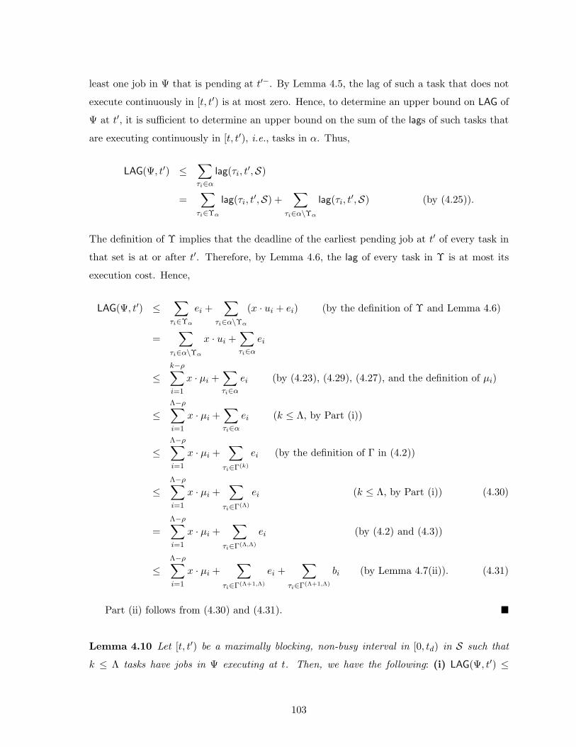
least one job in Ψ that is pending at t′−. By Lemma 4.5, the lag of such a task that does not

execute continuously in [t, t′) is at most zero. Hence, to determine an upper bound on LAG of

Ψ at t′, it is sufficient to determine an upper bound on the sum of the lags of such tasks that

are executing continuously in [t, t′), i.e., tasks in α. Thus,

LAG(Ψ, t′) ≤∑

τi∈α

lag(τi, t′,S)

=∑

τi∈Υα

lag(τi, t′,S) +

∑

τi∈α\Υα

lag(τi, t′,S) (by (4.25)).

The definition of Υ implies that the deadline of the earliest pending job at t′ of every task in

that set is at or after t′. Therefore, by Lemma 4.6, the lag of every task in Υ is at most its

execution cost. Hence,

LAG(Ψ, t′) ≤∑

τi∈Υα

ei +∑

τi∈α\Υα

(x · ui + ei) (by the definition of Υ and Lemma 4.6)

=∑

τi∈α\Υα

x · ui +∑

τi∈α

ei

≤k−ρ∑

i=1

x · µi +∑

τi∈α

ei (by (4.23), (4.29), (4.27), and the definition of µi)

≤Λ−ρ∑

i=1

x · µi +∑

τi∈α

ei (k ≤ Λ, by Part (i))

≤Λ−ρ∑

i=1

x · µi +∑

τi∈Γ(k)

ei (by the definition of Γ in (4.2))

≤Λ−ρ∑

i=1

x · µi +∑

τi∈Γ(Λ)

ei (k ≤ Λ, by Part (i)) (4.30)

=

Λ−ρ∑

i=1

x · µi +∑

τi∈Γ(Λ,Λ)

ei (by (4.2) and (4.3))

≤Λ−ρ∑

i=1

x · µi +∑

τi∈Γ(Λ+1,Λ)

ei +∑

τi∈Γ(Λ+1,Λ)

bi (by Lemma 4.7(ii)). (4.31)

Part (ii) follows from (4.30) and (4.31). �

Lemma 4.10 Let [t, t′) be a maximally blocking, non-busy interval in [0, td) in S such that

k ≤ Λ tasks have jobs in Ψ executing at t. Then, we have the following: (i) LAG(Ψ, t′) ≤

103

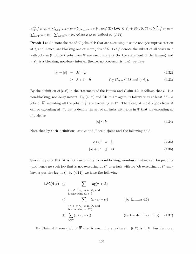
∑Λ−ρi=1 x ·µi +

∑


τi∈Π(Λ+1,Λ) bi, and (ii) LAG(Ψ, t′)+B(τ,Ψ, t′) <∑Λ−ρ

i=1 x ·µi +∑

τi∈Γ(M,Λ) ei +∑

τi∈Π(M,Λ) bi, where ρ is as defined in (4.21).

Proof: Let J denote the set of all jobs of Ψ that are executing in some non-preemptive section

at t, and, hence, are blocking one or more jobs of Ψ. Let β denote the subset of all tasks in τ

with jobs in J. Since k jobs from Ψ are executing at t (by the statement of the lemma) and

[t, t′) is a blocking, non-busy interval (hence, no processor is idle), we have

|J| = |β| = M − k (4.32)

≥ Λ + 1 − k (by Usum ≤ M and (4.6)). (4.33)

By the definition of [t, t′) in the statement of the lemma and Claim 4.2, it follows that t− is a

non-blocking, non-busy instant. By (4.32) and Claim 4.2 again, it follows that at least M − k

jobs of Ψ, including all the jobs in J, are executing at t−. Therefore, at most k jobs from Ψ

can be executing at t−. Let α denote the set of all tasks with jobs in Ψ that are executing at

t−. Hence,

|α| ≤ k. (4.34)

Note that by their definitions, sets α and β are disjoint and the following hold.

α ∩ β = ∅ (4.35)

|α| + |β| ≤ M (4.36)

Since no job of Ψ that is not executing at a non-blocking, non-busy instant can be pending

(and hence no such job that is not executing at t− or a task with no job executing at t− may

have a positive lag at t), by (4.14), we have the following.

LAG(Ψ, t) ≤∑

{τi ∈ τ |τi,j is in Ψ, andis executing at t−}

lag(τi, t,S)

≤∑

{τi ∈ τ |τi,j is in Ψ, andis executing at t−}

(x · ui + ei) (by Lemma 4.6)

≤∑

τi∈α

(x · ui + ei) (by the definition of α) (4.37)

By Claim 4.2, every job of Ψ that is executing anywhere in [t, t′) is in J. Furthermore,

104

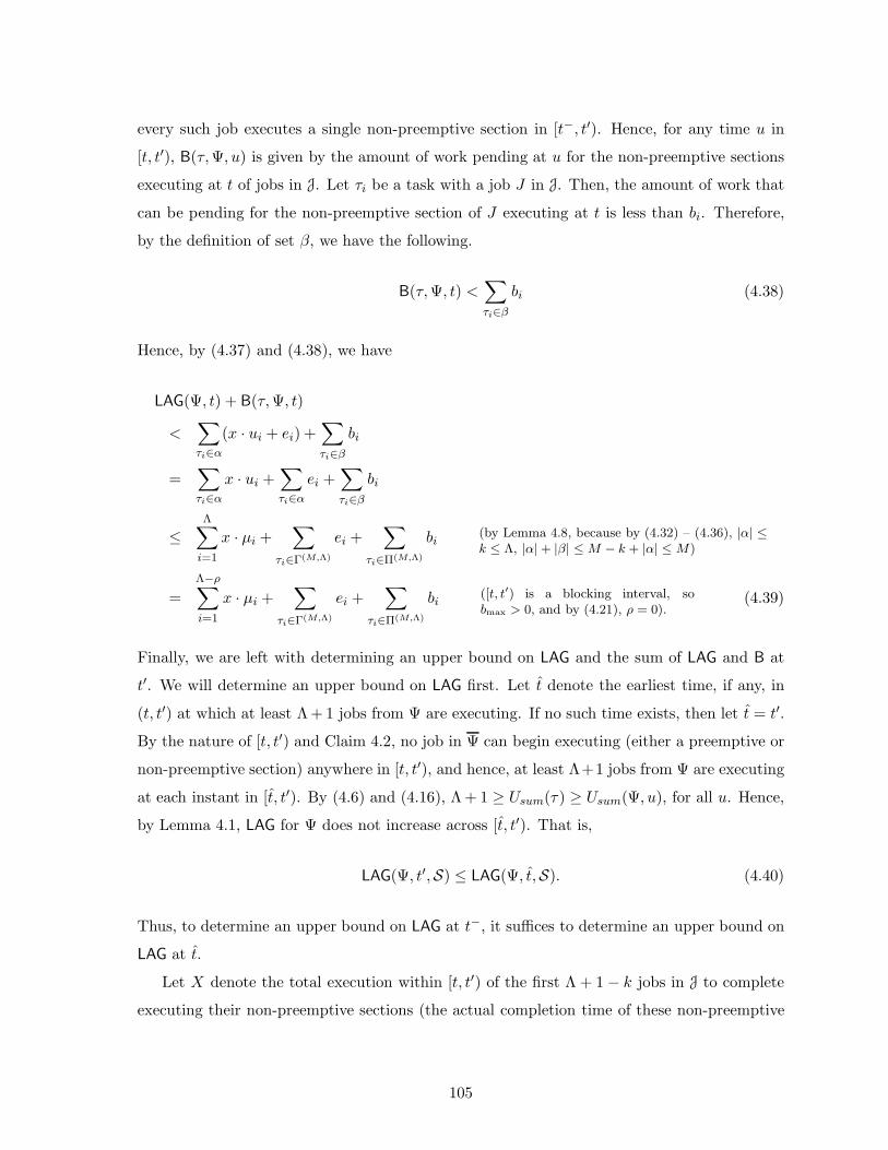
every such job executes a single non-preemptive section in [t−, t′). Hence, for any time u in

[t, t′), B(τ,Ψ, u) is given by the amount of work pending at u for the non-preemptive sections

executing at t of jobs in J. Let τi be a task with a job J in J. Then, the amount of work that

can be pending for the non-preemptive section of J executing at t is less than bi. Therefore,

by the definition of set β, we have the following.

B(τ,Ψ, t) <∑

τi∈β

bi (4.38)

Hence, by (4.37) and (4.38), we have

LAG(Ψ, t) + B(τ,Ψ, t)

<∑

τi∈α

(x · ui + ei) +∑

τi∈β

bi

=∑

τi∈α

x · ui +∑

τi∈α

ei +∑

τi∈β

bi

≤Λ∑

i=1

x · µi +∑

τi∈Γ(M,Λ)

ei +∑

τi∈Π(M,Λ)

bi(by Lemma 4.8, because by (4.32) – (4.36), |α| ≤k ≤ Λ, |α| + |β| ≤ M − k + |α| ≤ M)

=

Λ−ρ∑

i=1

x · µi +∑

τi∈Γ(M,Λ)

ei +∑

τi∈Π(M,Λ)

bi([t, t′) is a blocking interval, sobmax > 0, and by (4.21), ρ = 0).

(4.39)

Finally, we are left with determining an upper bound on LAG and the sum of LAG and B at

t′. We will determine an upper bound on LAG first. Let t denote the earliest time, if any, in

(t, t′) at which at least Λ + 1 jobs from Ψ are executing. If no such time exists, then let t = t′.

By the nature of [t, t′) and Claim 4.2, no job in Ψ can begin executing (either a preemptive or

non-preemptive section) anywhere in [t, t′), and hence, at least Λ+1 jobs from Ψ are executing

at each instant in [t, t′). By (4.6) and (4.16), Λ + 1 ≥ Usum(τ) ≥ Usum(Ψ, u), for all u. Hence,

by Lemma 4.1, LAG for Ψ does not increase across [t, t′). That is,

LAG(Ψ, t′,S) ≤ LAG(Ψ, t,S). (4.40)

Thus, to determine an upper bound on LAG at t−, it suffices to determine an upper bound on

LAG at t.

Let X denote the total execution within [t, t′) of the first Λ + 1 − k jobs in J to complete

executing their non-preemptive sections (the actual completion time of these non-preemptive

105

sections is immaterial). Note that X is well defined because by (4.33), |J| ≥ Λ + 1 − k holds.

Because [t, t′) is maximally blocking, no processor is idle in [t, t), and because k jobs in Ψ are

executing at t, at least k jobs execute at every instant in [t, t′). Also, when a job in J completes

executing its non-preemptive section in [t, t′), the processor it executed on is allocated to a

waiting job in Ψ. Hence, the total time allocated to jobs in Ψ in [t, t), A(S,Ψ, t, t), is equal to

k · (t− t) + (Λ + 1− k) · (t− t)−X = (Λ + 1) · (t− t)−X. In PSτ , jobs in Ψ could execute for

at most Usum(τ) · (t − t) time, i.e., A(PSτ ,Ψ, t, t) ≤ Usum(τ) · (t − t) ≤ (Λ + 1) · (t − t). (The

second inequality is by (4.6).) Therefore, by (4.12),

LAG(Ψ, t) = LAG(Ψ, t) + A(PSτ ,Ψ, t, t) − A(S,Ψ, t, t)

≤ LAG(Ψ, t) + (Λ + 1) · (t − t) − (Λ + 1) · (t − t) + X

= LAG(Ψ, t) + X. (4.41)

Let β(Λ+1−k) denote the subset of Λ+1−k tasks whose jobs in J complete executing their non-

preemptive sections the earliest. (Again, by (4.33), |J| ≥ Λ + 1 − k.) Then, by the discussion

thus far,

LAG(Ψ, t′,S)

≤ LAG(Ψ, t,S) (by (4.40))

≤ LAG(Ψ, t) + X (by (4.41))

≤∑

τi∈α

(x · ui + ei) +∑

τi∈β(Λ+1−k)

bi (by (4.37) and the definition of X)

≤k∑

i=1

x · µi +∑

τi∈α

ei +∑

τi∈β(Λ+1−k)

bi (by (4.34) and the definition of µi)

≤Λ∑

i=1

x · µi +∑

τi∈Γ(Λ+1,Λ)

ei +∑

τi∈Π(Λ+1,Λ)

bi

(by Lemma 4.8; note that α and β(Λ+1−k)

are disjoint, |α| ≤ k ≤ Λ holds by (4.34),and because |β(Λ+1−k)| = Λ + 1 − k, |α| +|β(Λ+1−k)| ≤ Λ + 1 holds as well)

≤Λ−ρ∑

i=1

x · µi +∑

τi∈Γ(Λ+1,Λ)

ei +∑

τi∈Π(Λ+1,Λ)

bi (by (4.21), ρ = 0 since bmax > 0).

The above establishes Part (i) of the lemma.

To determine an upper bound on LAG plus B at t′, let X ′ ≤ B(τ,Ψ, t) denote the total

amount of time that jobs in J execute on all M processors in [t, t′). Then, the total time

106

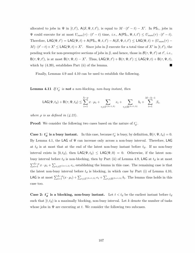
allocated to jobs in Ψ in [t, t′), A(S,Ψ, t, t′), is equal to M · (t′ − t) − X ′. In PSτ , jobs in

Ψ could execute for at most Usum(τ) · (t′ − t) time, i.e., A(PSτ ,Ψ, t, t′) ≤ Usum(τ) · (t′ − t).

Therefore, LAG(Ψ, t′) = LAG(Ψ, t) + A(PSτ ,Ψ, t, t′) − A(S,Ψ, t, t′) ≤ LAG(Ψ, t) + (Usum(τ) −M) · (t′− t)+X ′ ≤ LAG(Ψ, t)+X ′. Since jobs in J execute for a total time of X ′ in [t, t′), the

pending work for non-preemptive sections of jobs in J, and hence, those in B(τ,Ψ, t′) at t′, i.e.,

B(τ,Ψ, t′), is at most B(τ,Ψ, t) − X ′. Thus, LAG(Ψ, t′) + B(τ,Ψ, t′) ≤ LAG(Ψ, t) + B(τ,Ψ, t),

which by (4.39), establishes Part (ii) of the lemma. �

Finally, Lemmas 4.9 and 4.10 can be used to establish the following.

Lemma 4.11 If t−d is not a non-blocking, non-busy instant, then

LAG(Ψ, td) + B(τ,Ψ, td) ≤Λ−ρ∑

i=1

x · µi +∑

τi∈Γ(Λ+1,Λ)

ei +∑

τi∈Π(Λ+1,Λ)

bi +

M−Λ−1∑

i=1

βi,

where ρ is as defined in (4.21).

Proof: We consider the following two cases based on the nature of t−d .

Case 1: t−

d is a busy instant. In this case, because t−d is busy, by definition, B(τ,Ψ, td) = 0.

By Lemma 4.1, the LAG of Ψ can increase only across a non-busy interval. Therefore, LAG

at td is at most that at the end of the latest non-busy instant before td. If no non-busy

interval exists in [0, td), then LAG(Ψ, td) ≤ LAG(Ψ, 0) = 0. Otherwise, if the latest non-

busy interval before td is non-blocking, then by Part (ii) of Lemma 4.9, LAG at td is at most∑Λ−ρ

i=1 x · µi +∑

τi∈Γ(Λ+1,Λ) ei, establishing the lemma in this case. The remaining case is that

the latest non-busy interval before td is blocking, in which case by Part (i) of Lemma 4.10,

LAG is at most∑Λ−ρ

i=1 (x · µi) +∑


τi∈Π(Λ+1,Λ) bi. The lemma thus holds in this

case too.

Case 2: t−

d is a blocking, non-busy instant. Let t < td be the earliest instant before td

such that [t, td) is a maximally blocking, non-busy interval. Let k denote the number of tasks

whose jobs in Ψ are executing at t. We consider the following two subcases.

107

Subcase 2(a): LAG(Ψ, td) > LAG(Ψ, t) or k ≤ Λ. If LAG(Ψ, td) > LAG(Ψ, t) holds, then

by Claim 4.3, k ≤ Λ holds. Hence, in either case, by Part (ii) of Lemma 4.10, we have

LAG(Ψ, td) + B(τ,Ψ, td) <

Λ−ρ∑

i=1

x · µi +∑

τi∈Γ(M,Λ)

ei +∑

τi∈Π(M,Λ)

bi

≤Λ−ρ∑

i=1

x · µi +∑

τi∈Γ(Λ+1,Λ)

ei +∑

τi∈Π(Λ+1,Λ)

bi +

M−Λ−1∑

i=1

βi,

establishing the lemma for this subcase. The second inequality follows from Lemma 4.7(i)

(because M ≥ Λ + 1, by (4.6) and M ≤ Usum).

Subcase 2(b): k > Λ and LAG(Ψ, td) ≤ LAG(Ψ, t). By the conditions of this subcase, it

follows that LAG at td is bounded from above by the LAG at the end of the latest non-blocking

or blocking non-busy interval before t across which LAG increases. If no such interval exists,

then by Lemma 4.1, LAG(τ, td) ≤ LAG(τ, 0) = 0. Otherwise, (as with Case 1) by Part (ii) of

Lemma 4.9 and Part (i) of Lemma 4.10, we have

LAG(Ψ, td) ≤Λ−ρ∑

i=1

x · µi +∑

τi∈Γ(Λ+1,Λ)

ei +∑

τi∈Π(Λ+1,Λ)

bi. (4.42)

Since k > Λ holds, at most M − Λ − 1 jobs from Ψ can be executing at t, and by Claim 4.2,

at most M − Λ − 1 such jobs can be executing at t−d as well. The amount of time for which

such a job of task τi can execute past td in its non-preemptive section is less than bi. Thus,

B(τ,Ψ, td) <∑M−Λ−1

i=1 βi holds. Therefore, by (4.42), LAG(Ψ, td) + B(τ,Ψ, td) <∑Λ−ρ

i=1 x ·µi +∑



i=1 βi holds. �

Lemma 4.12 If t−d is a non-blocking, non-busy instant, then tardiness(τ`,j) ≤ x + e`.

Proof: If t−d is a non-blocking, non-busy instant, then at most M − 1 tasks have pending

jobs at t−d in Ψ and each of these tasks is executing at t−d . Let α denote the set of all such

tasks. Since no job with a deadline at or before td can be released at or after td, a task in α

cannot be preempted until all its jobs in Ψ complete execution, i.e., each task in α executes

continuously until all its jobs in Ψ complete execution. If τ`,j completes execution before td,

then its tardiness is zero. Otherwise, τ` is in α, and by Lemma 4.6, its lag at td is at most

x · u` + e`. Since the deadline of τ`,j is at td, no job of τ` with a deadline after td is released

108

before td. Jobs with release times after td receive no allocation before td in PSτ , even if their

eligibility times are earlier. Hence, lag for such jobs of τ` is zero at td. Thus, τ`’s lag at td (given

by the sum of the lags of all its jobs) is at most the amount of work pending for its jobs in Ψ.

Because τ` is in α, it executes continuously until all its jobs in Ψ, which includes τ`,j, complete

execution. The latest completion time is given by td+ lag(τ`, td,S) ≤ td+x·u`+e` ≤ td+x+e`,

and hence, the tardiness of τ`,j is at most x + e`. �

4.3.2.3 Finishing Up (Step (S3))

If td is a non-blocking, non-busy instant, then Lemma 4.12 contradicts (P1). Otherwise, by

Lemma 4.3 and (P1), LAG(τ, td,S) + B(Ψ, τ, td,S) > M · x + e`. Therefore, by Lemma 4.11,

M · x + e` <∑Λ−ρ

i=1 x · µi +∑



i=1 βi, i.e.,

x <

∑



i=1 βi − e`


≤∑



i=1 βi − emin


,

which contradicts (4.20). Thus, Theorem 4.1 below follows.

Theorem 4.1 Let τ be a sporadic task system with non-preemptable segments and Usum ≤ M .

Then, on M processors, EDF-P-NP ensures a tardiness of at most x + ek to every task τk in

τ , where x is as defined by (4.20).

If no task has non-preemptable segments, then EDF-P-NP reduces to g-EDF (fully-preemptive

global EDF). In such a case, bi = βi = 0, for all i. Hence, bmax = 0, and by Lemma 4.4, ρ ≥ 1.

Further, ei − bi = ei, and hence, Γ(Λ+1,Λ) is simply a subset of Λ tasks of τ with the highest

execution costs, i.e., Γ(Λ+1,Λ) = Γ(Λ). Therefore, a tardiness bound under g-EDF is given by

the following corollary to Theorem 4.1.

Corollary 4.1 g-EDF ensures a tardiness bound of

∑Λi=1 εi − emin

M −∑Λ−1i=1 µi

+ ek (4.43)

to every task τk of a sporadic task system τ with Usum ≤ M .

109

A sufficient condition on the individual task utilizations for a given tardiness bound under g-

EDF that places no restriction on the total utilization can be derived from the above corollary,

as given below.

Corollary 4.2 g-EDF ensures a tardiness of at most xp + ek for every task τk of a sporadic

task system τ on M processors if the sum of the utilizations of the Λ − 1 tasks with highest

utilizations,∑Λ−1

i=1 µi, is at most M −∑Λ

i=1 εi+emin

xpand Usum(τ) ≤ M .

Proof: By Corollary 4.1, the tardiness for task τk of τ in a g-EDF schedule is at most∑Λ

i=1 εi−emin

M−∑Λ−1

i=1 µi+ek. Therefore, a tardiness not exceeding xp+ek can be guaranteed if

(∑Λ

i=1 εi)−emin

M−∑Λ−1

i=1 µi+

ek ≤ xp + ek holds. On rearranging the terms, we arrive at the condition in the corollary. �

Similarly, EDF-P-NP reduces to g-NP-EDF (fully-non-preemptive EDF) if bi = ei, for all i.

Therefore, Γ(Λ+1,Λ) ∪ Π(Λ+1,Λ) = Γ(Λ+1). Further, by (4.21), ρ = 0 holds. In this case, the

tardiness bound of Theorem 4.1 reduces to the following.

Corollary 4.3 On M processors, g-NP-EDF ensures a tardiness bound of

∑Λ+1i=1 εi +

∑M−Λ−1i=1 βi − emin

M −∑Λi=1 µi

+ ek

to every task τk of a sporadic task system τ with Usum ≤ M .

4.3.3 Tardiness Bound under g-EDF for Two-Processor Systems

If 1 < Usum ≤ 2, then the tardiness bound under g-EDF given by Corollary 4.1 for task τk

under two processors (i.e., when M = 2) is (emax − emin)/2+ ek. However, an improved bound

of emax/2 + ek/2 can be ensured if we note that LAG + B at td, as given by Lemma 4.11, is

at most emax, which is independent of x. This improved bound is derived in the following

theorem.

Theorem 4.2 On two processors, g-EDF ensures a tardiness of at most emax+ek

2 for every task

τk of every sporadic task system with Usum ≤ 2.

Proof: Suppose that the theorem does not hold. Then, there exists a concrete instantiation

τ of a non-concrete task system with Usum ≤ 2 such that τ`,j is a job of task τ` in τ , S is a

g-EDF schedule for τ , td = d`,j, and (P1)–(P4) (defined in the beginning of Section 4.3.2) hold,

where x = emax−e`

2 . As with the general case, if t−d is a non-blocking, non-busy instant, then

110

Lemma 4.12 contradicts (P1). Otherwise, by Lemmas 4.11 and 4.4, and because bi = 0, for all

i, we have

LAG(τ, td,S) + B(Ψ, τ, td,S) ≤ emax. (4.44)

By (P1), tardiness(τ`,j) > x + e`. Hence, by the contrapositive of Lemma 4.3, we have

LAG(τ, td,S)+B(Ψ, τ, td,S) > 2 ·x+e`, which, by (4.44), implies that emax > 2 ·x+e` = emax,

a contradiction. The theorem, therefore, follows. �

4.3.4 Improving Accuracy and Speed

In this subsection, we discuss possible improvements to the accuracy of the tardiness bounds

of g-EDF and g-NP-EDF given in Corollaries 4.1 and 4.3, respectively, and the time required

to compute them. We will refer to the bounds given by Corollaries 4.1 and 4.3 as EDF-BASIC

and NP-EDF-BASIC, respectively.

Improving accuracy. If the time taken to compute a tardiness bound, or sufficient task

utilizations for a given tardiness bound, is not a concern, then some improvement to the values

may be possible by relaxing a pessimistic assumption that we make in Lemmas 4.9 and 4.10.

We not only assume that the tasks that are executing at the end of the non-blocking, non-

busy interval in Lemma 4.9, or just before the beginning of the blocking, non-busy interval in

Lemma 4.10, have the highest utilizations, but also that they have the highest execution costs.

For g-EDF, this can be relaxed by sorting tasks by non-increasing order of x · uk + ek (where,

as defined in (P4), the tardiness of τk is at most x + ek) and by using the utilizations and

execution costs of the top Λ − 1 tasks in the expression in Corollary 4.1. (The Λth execution

cost should be taken as the maximum of the execution costs of the remaining tasks.) If x is

known (i.e., when determining utilization restrictions for a given tardiness), as in applying

Corollary 4.2, then this procedure is straightforward. Nevertheless, even when seeking x (i.e.,

when determining a tardiness bound), as in Corollary 4.1, an iterative procedure could be

used. In this iterative procedure, the bound given by EDF-BASIC will be used as the initial

value for x. This initial value will then be used to determine the set of tasks whose utilizations

and execution costs should be used in improving x. The procedure should be continued until

the task set converges. (It is easy to show that convergence is guaranteed.) We will refer to the

bound computed using such an iterative procedure as EDF-ITER. This procedure is illustrated

in the example below.

111

Example 4.2. Let τ be a task system consisting of the following eight tasks with Usum = 4.0

scheduled under g-EDF on M = 4 processors: τ1(15, 150)–τ4(15, 150), τ5(9, 10)–τ8(9, 10). For

this task set, µ1 = µ2 = 0.9, ε1 = ε2 = ε3 = 15, and Λ = 3. Therefore, a tardiness bound for

τk obtained using EDF-BASIC is (45 − 9)/(4 − 18/10) + ek, which equals 360/22 + ek. Thus,

x ≈ 16.36. Computing x·uk+ek for each task τk, we obtain values of 16.636 for tasks τ1, . . . , τ4,

and 23.727 for τ5, . . . , τ8. Hence, the two tasks with the highest values for x ·uk +ek are τ5 and

τ6. Using the execution costs and utilizations of τ5 and τ6 and 15 as the Λth execution cost, we

obtain an improved value of 10.9 for x, which is more than 5 units less than the initial value.

The set of tasks with the highest value for x · uk + ek is not altered in the next iteration, and

so, the procedure terminates.

A similar procedure can be used for computing an improved bound for g-NP-EDF also,

except that Λ tasks τk with the highest values for x · uk + ek have to be considered.

Improving computation time. Computing the tardiness bound or determining utilization

restrictions on tasks for a given bound involves selecting O(M) tasks with the highest utiliza-

tions, and O(M) tasks with the highest execution costs (or the highest values for ei − bi), and

summing these values. Because worst-case [38] and expected [58, 64] linear-time selection algo-

rithms are known, these are O(N +M) computations. If speed is a concern, as in online admis-

sion tests, and if umax and emax are known, then O(1) computations, which assume a utilization

of umax and an execution cost of emax for each of the M−1 tasks, can be used, at the expense of

more pessimistic values. Under this assumption, tardiness bounds under g-EDF and g-NP-EDF

are ((M−1)emax−emin)/(M −(M−2)umax)+ei and (M ·emax−emin)/(M −(M−1)umax)+ei,

respectively, for each task τi. Similarly, for a tardiness bound of x+ei for every τi under g-EDF,

it is sufficient that umax be at most (M · x − (M − 1)emax + emin)/((M − 2)x). We will refer

to the bounds computed using umax and emax as EDF-FAST and NP-EDF-FAST, respectively.

Tightness of the bound. As discussed in the introduction, we do not believe that our

results are tight for either g-EDF or g-NP-EDF. It can be verified that for both g-EDF and

g-NP-EDF, the bounds derived are increasing functions of M . In addition, when Usum = M ,

the g-EDF (resp., g-NP-EDF) bound is an increasing function of the average of the highest

M − 2 (resp., M − 1) task utilizations, denoted uavg(M − 2) (resp., uavg(M − 1)), and the

average of the highest M − 1 (resp., M) task execution costs, denoted eavg(M − 1) (resp.,

eavg(M)). Approximate plots of the tardiness bounds computed for g-EDF and g-NP-EDF for

112

0 0.2 0.4 0.6 0.8 10

10

20

30

40

50

60

70

80

90

100

Tardiness bound by U−avg(M−1) for g−NP−EDF

Average Utilization U−avg(M−1)

Max

imum

Tar

dine

ss (

mul

tiple

s of

e−a

vg(M

))

M=2M=3M=4M=8M=16M=20M=30M=40M=50M=100

(a)

0 0.2 0.4 0.6 0.8 10

10

20

30

40

50

60

70

80

90

100

Tardiness Bound by U−avg(M−2) for g−EDF

Average Utilization U−avg(M−2)

Max

imum

Tar

dine

ss (

Mul

tiple

s of

e−a

vg(M

−1))

M=3M=4M=8M=16M=20M=30M=40M=50M=100

(b)

Figure 4.3: Tardiness bounds for (a) g-EDF and (b) g-NP-EDF for varying number of pro-cessors (M) as functions of average task utilization (uavg). Values of M are higher for curveshigher up.

varying values of M and uavg are shown in Figures 4.3 and 4.4. The plotted bounds are in

multiples of eavg(M − 1) for g-EDF and eavg(M) for g-NP-EDF. As can be seen from the plots,

the bounds are quite reasonable unless both M and uavg are both high. For instance, for

g-EDF, if uavg is at most 0.75 (resp., 0.5), then the bound guaranteed is approximately at most

113

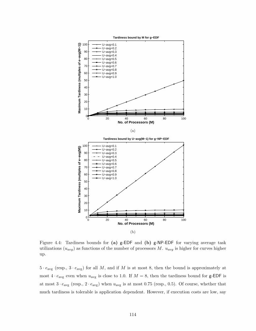
0 20 40 60 80 1000

10

20

30

40

50

60

70

80

90

100

Tardiness bound by M for g−EDF

No. of Processors (M)

Max

imum

Tar

dine

ss (

mul

tiple

s of

e−a

vg(M

−1))

U−avg=0.1U−avg=0.2U−avg=0.3U−avg=0.4U−avg=0.5U−avg=0.6U−avg=0.7U−avg=0.8U−avg=0.9U−avg=1.0

(a)

0 20 40 60 80 1000

10

20

30

40

50

60

70

80

90

100

Tardiness bound by U−avg(M−1) for g−NP−EDF

No. of Processors (M)

Max

imum

Tar

dine

ss (

mul

tiple

s of

e−a

vg(M

))

U−avg=0.1U−avg=0.2U−avg=0.3U−avg=0.4U−avg=0.5U−avg=0.6U−avg=0.7U−avg=0.8U−avg=0.9U−avg=1.0

(b)

Figure 4.4: Tardiness bounds for (a) g-EDF and (b) g-NP-EDF for varying average taskutilizations (uavg) as functions of the number of processors M . uavg is higher for curves higherup.

5 · eavg (resp., 3 · eavg) for all M , and if M is at most 8, then the bound is approximately at

most 4 · eavg even when uavg is close to 1.0. If M = 8, then the tardiness bound for g-EDF is

at most 3 · eavg (resp., 2 · eavg) when uavg is at most 0.75 (resp., 0.5). Of course, whether that

much tardiness is tolerable is application dependent. However, if execution costs are low, say

114

of the order of a few milliseconds, as can be expected with modern processors, then in many

cases, the tardiness bounds guaranteed can be expected to be within limits.

Though the bounds may not be tight, in general, we can show that our result for g-EDF

is within approximately emax of tardiness possible in the worst case for small values of umax.

For this, consider a task system τ that consists of a primary task τ1(e1, p1) and (M − u1)p1/δ

auxiliary tasks. Let δ � e1 and p1 be the execution cost and period, respectively, of each

auxiliary task. Let δ divide (M − u1) evenly. The total utilization of this task system is

(δ/p1)× ((M − u1)p1/δ) + u1 = M . Suppose that the first job of each task is released at time

0 and suppose that the first job of every auxiliary task is scheduled before τ1,1 and executes

for a full δ time units. In such a schedule, the auxiliary jobs will execute continuously until

time ( (M−u1)p1

δ × δ)/M = p1 − e1/M on each processor. Hence, τ1 will not begin executing

until time p1 − e1/M , and hence would not complete until p1 + e1 · (1 − 1/M) for a tardiness

of e1 · (1 − 1/M) = e1 · ((M − 1)/M). By choosing e1 = M , this tardiness can be made

to equal e1 − 1. In this example, emax = e1, and hence tardiness is at least emax − 1. In

the example schedule described above, tardiness is independent of u1 = e1/p1, and hence,

holds even when u1 is arbitrarily small, which is possible by choosing p1 � e1. Note that

when umax is arbitrarily low, a tardiness bound under g-EDF computed using EDF-FAST

is around ((M − 1) · emax − emin)/M + emax, which is ((M − 1) · M − δ)/M + M for this

example (because emax = M). This bound differs from the observed tardiness of M − 1

by M − δ/M , which is at most M = emax. (The bound computed using EDF-BASIC is

(M + (M − 3) · δ)/(M − u1 − (M − 3) · u1 · δ/M) + M and differs from the observed tardiness

by (M + (M − 3) · δ)/(M − u1 − (M − 3) · u1 · δ/M) + 1, which can be verified to be at most

(2 + δ)M/(M − 1) for u1 ≤ 11+δ .)

Tightness of the g-EDF bound on two processors. By Theorem 4.2, tardiness is at

most (emax + e`)/2 for task τ` on two-processor systems. The following is an example that

shows that this result is reasonably tight. Let τ1(1, 2), τ2(1, 2), and τ3(2k + 1, 2k + 1), where

k ≥ 1, be three periodic tasks all of whose first jobs are released at time zero. If deadline

ties are resolved in favor of τ1 and τ2 over τ3, then on two processors, tardiness for jobs of τ3

can be as high as 2k time units. (If τ3 is favored, then its jobs can miss by 2k − 1.) Such a

schedule for a task system with k = 7 is shown in Figure 4.5. In this schedule, the sixth job

of τ3, with deadline at time 90, completes executing at time 104, and hence, has a tardiness

of 14 time units, which is emax − 1. The schedule pattern in [73, 104) repeats after time

115

deadline miss

Allocations on Processor 1 Allocations on Processor 2L E G E N D :

1(1,2)τ

τ2(1,2)

5

deadline miss

deadline miss

0 10 15 20 30 35 40 45 50 55 60 65 70 75 80 85 90 95 10025

τ3(15,15)

deadline miss

deadline miss deadline miss

Figure 4.5: A schedule under g-EDF for the first few jobs of the task system indicated on twoprocessors. Tardiness for the sixth job of τ3 is 14 time units, which is emax − 1.

104, and so tardiness converges to 14 time units after time 104. For this task set, estimated

tardiness is emax = 2k + 1, and for large k, the difference between the estimated and actual

tardiness is negligible. The above example can be tweaked to generate other task sets in which

the maximum utilization is much less than unity, but which can yet miss their deadlines by

emax−1 time units under g-EDF. A task system with the following seven tasks is one example:

τ1(1, 4), . . . , τ6(1, 4), τ7(2k + 1, 4k + 2), where k ≥ 1. In this example, τ7 can miss deadlines by

up to 2k time units, and the remaining tasks by up to k time units. (Note that 2k = emax − 1

and k = emax+e`

2 − 1, for 1 ≤ ` ≤ 6.)

An empirical evaluation of the accuracy of the bounds is provided in Section 4.5. Interest-

ingly, we have found that tardiness under g-EDF can exceed emax even for task systems with

umax near 1/2. The following is one such task set: τ1(1, 2), . . . , τ4(1, 2), τ5(1, 5), . . . , τ7(1, 5),

τ8(1, 11), τ9(34, 110), τ10(23, 63), τ11(7, 18),τ12(7, 18), τ13(3, 7),τ14(3, 7). The total utilization

of this task set is five. When scheduled on five processors with deadline ties resolved using

task indices, a job of τ9 misses its deadline at time 7295 by 35 > 34 = emax time units. (The

EDF-BASIC and EDF-ITER bounds for this task set are 54 and 51.78, respectively.) Hence, the

best bound possible for an arbitrary task set definitely exceeds emax.

4.4 A Useful Task Model Extension

In this section, we consider a useful extension to the sporadic task model, and discuss how

a tardiness bound can be derived under it. We argue that the derivation of such a bound

involves only minimal changes to that used for the base model (i.e., the model described in

Section 4.2).

As explained later, the extension that we consider can be used to model certain dynamic

116

task behaviors. In this extended model, the number of tasks associated with the task system

is allowed to exceed N and the total utilization of all tasks is allowed to exceed M . (The

number of tasks could potentially be infinite.) However, to prevent overload, at any given

time, only a subset of tasks whose total utilization is at most M is allowed to be active,5 i.e.,

is allowed to release jobs. Additionally, we allow the final job of a task to halt at some time

th before its deadline, provided that the allocation that the job receives in the actual schedule

is at most the allocation it receives up to th in a PS schedule and the job is not executing in

a non-preemptive segment at th. When a job halts, its execution cost is altered to equal the

amount of time that the job actually executed for in the actual schedule up to th. Hence, the

halting job receives no allocation in the PS schedule after th, even if its deadline is after th.

At any time t, each task τi can be in one of the following states.

• Active, if the first job of τi is released at or before t, the deadline of its final job is after

t, and its final job has not halted at or before t. A task whose final job has its deadline

at or before t is not considered active at t even if the final job is pending at t.

• Inactive, if the release time of the first job of τi is after t.

• Terminated , if the deadline of τi’s final job is before t.

• Halted , if the final job has halted but its deadline has not elapsed.

As can be easily seen, a task that is either inactive or terminated at time t cannot have active

jobs at t. Also, though the deadline of a halted job may be after its halting time, the job

receives no allocation in the PS schedule after it halts.

The set of all tasks associated with the task system is partitioned into N task classes

such that the following hold: (i) active intervals are disjoint for every two tasks in each class

and (ii) tasks within a class are governed by precedence constraints, i.e., the first job of a

task cannot begin execution until all jobs of all tasks with earlier active intervals in its class

have completed execution. The second requirement implies that tasks that are not bound

by precedence constraints should belong to different classes even if their active intervals are

disjoint.

5The term active is overloaded in that it was defined previously for jobs (see Definition 4.1 in Section 4.3.1).The definition of this term is different for tasks, and active tasks are not to be confused with active jobs.Specifically, a task can be considered to be active at some time even if it has no active job at that time.

117

τ (2,4)1

τ (2,3)9

τ (1,6)3

τ (5,6)5

τ (1,6)7

τ (1,3)2

τ (3,6)4

τ (1,3)6

τ (1,2)8

τ (2,4)1

τ (1,3)2

τ (1,6)3

τ (3,6)4

τ (5,6)5

τ (1,3)6

τ (1,6)7

τ (1,2)8

(b)(a)

. . .

. . .

. . .

0 2 4 6 8 10 12 14 16 18 20

time

. . .

. . .

. . .

. . .

. . .

. . .

0 2 4 6 8 10 12 14 16 18 20

time

Terminated

Terminated

Terminated

Inactive

Inactive

halted

Terminated

Terminated

Terminated

Terminated

Terminated

Inactive

Inactive

InactiveInactive

L E G E N D : Allocations on Processor 1 Allocations on Processor 2

Figure 4.6: Example g-EDF schedules for extended sporadic task systems. (a) No job halts.(b) The fourth job of τ1 halts at time 14.

Examples of task systems that conform to the proposed extension are shown in Figure 4.6.

In each example, tasks that belong to different classes are demarcated using solid lines; those

within a class are separated using dashed lines. An initial few jobs are shown for each task.

There are eight tasks and six task classes in the task system in inset (a). Each task becomes

active at the release time of its first job. Tasks whose jobs are followed by ellipsis are still

active at time 18 and may be active beyond that time. Termination times for the remaining

tasks are given by the deadlines of their final jobs. For example, τ2 and τ3 terminate at time

6, and τ6 is active in the interval [12,∞). It can be verified that the total utilization of all the

active tasks at any instant is 2. Note that since τ5 and τ6 are in the same class, τ6,1 cannot

118

τ3(3,4)

τ4(6,8)

τ5(5,12)

τ6(1,6)

τ1(6,9) τ

2(2,3)



L E G E N D

0 4 8 12 16 20 24

time

Figure 4.7: Example application of the extended task model to tasks with variable per-jobexecution costs.

begin execution until both jobs of τ5 have completed executing. Hence, at time 13, the fourth

job of τ1 is scheduled even though its deadline (which is at time 16) is later than that of τ6,1

(which is at time 15). Inset (b) shows an example wherein a job is halted before its deadline.

In this example, at time 14, the fourth job of τ1, τ1,4, is halted, and a new task, τ9, which

belongs to the same class as τ1, becomes active. At time 14, τ1,4 receives equal allocations (of

one time unit) in both the g-EDF and PS schedules, and hence, halting is permissible.

Applications. The extended task model can readily be used to model tasks whose job exe-

cution costs vary but whose utilizations remain unchanged. An example is shown in Figure 4.7.

The task system in this example has two tasks with fixed per-job execution costs and two with

variable execution costs. The first variable execution-cost task has a utilization of 2/3, an

execution requirement of six for its first two jobs, and two, for later jobs. The second such

task has a utilization of 3/4, an execution requirement of three for its first three jobs, and

six, for later jobs. Both the tasks can be represented using task classes of the extended task

model. In Figure 4.7, tasks τ1 and τ2 belong to the first task class. τ1 is active in the interval

[0, 18) and τ2 becomes active at time 18. Similarly, tasks τ3 and τ4 together model the second

variable execution-cost task.

The extended task model can also be used with dynamic tasks whose utilizations can vary

with time. In particular, a single task with a varying utilization can be modeled as a class of

potentially infinite tasks, each with a non-changing utilization. Such an approach has been

considered for scheduling dynamic task systems under g-EDF and g-NP-EDF in [37].

119

Tardiness bounds. The approach used for the base model can be used to derive a tardiness

bound for the extended model if each task class of the extended model is treated as a distinct

task of the base model. For clarity, we will initially assume that no job halts. Letting τC`

denote task class ` (the superscript C is used to distinguish a task from a task class), in

Lemma 4.6, the lag for τC` can easily be shown to be at most x ·maxτi∈τC

ùi + ek,q, where τk,q

is the earliest pending job of any of the tasks in τC` . Note that in a non-blocking, non-busy

interval with continually increasing LAG, as considered in Lemma 4.9, at most Λ task classes

can have pending jobs. Letting uC`

def= maxτi∈τC

ùi and eC

`def= maxτi∈τC

è`, it can be verified

that Lemmas 4.9 and 4.10 directly apply to the extended model (i.e., hold word for word) if

each task class is considered as a task and a C superscript is added to the various terms. (µCi

and εCi for all 1 ≤ ı ≤ N are defined for task classes in a straightforward manner). Hence,

the tardiness bounds derived hold if the maximum utilization and execution cost of each task

class are used instead of individual task utilizations and execution costs.

We now discuss why halting is not of issue. Recall that a job can halt only if the allocation

to it in the PS schedule is no less than the allocation it receives in the actual schedule. Further,

the actual execution cost of the halting job is altered to equal the allocation the job receives in

the actual schedule. Hence, the allocation to the job in the PS schedule can also retroactively

be altered to equal its actual execution cost. Further, since the job will receive no allocation

in the PS schedule after it halts, it is safe to reclaim the utilization of the halting task and

activate some other task. That is, there is no risk of overload (i.e., Usum will not exceed M),

which can adversely impact other tasks, in the interval spanning the job halting time and job

deadline. Finally, by definition, a job can halt only before its deadline and is not pending when

it halts. Therefore, because allocations in the PS schedule are altered as described above, the

tardiness and lag of a job are zero when the job halts. Hence, lag bounds derived for task

classes are not worsened even if its jobs halt. Also, since a job cannot halt in a non-preemptive

segment, bounds on blocking times are not altered.

4.5 Simulation-Based Evaluation

In this section, we describe the results of two sets of simulation experiments conducted using

randomly-generated task sets to evaluate the accuracy of the tardiness bounds for g-EDF and

g-NP-EDF derived in Section 4.3.

The first set of experiments compares the tardiness bounds given by EDF-BASIC and NP-

120

EDF-BASIC and their fast (EDF-FAST and NP-EDF-FAST) and iterative (EDF-ITER and NP-

EDF-ITER) variants for 4 and 8 processors (M). For each M , 106 task sets were generated. For

each task set, new tasks were added as long as Usum was less than M and a final task was added

so that Usum equalled M . For each task τi, first its utilization ui was generated as a uniform

random number between (0, y], where y was fixed at 0.1 for the first 100, 000 task sets, and

was incremented in steps of 0.1 for every 100, 000 task sets. τi’s execution cost was chosen as a

uniform random number in the range (0, 20]. For each task set, the maximum tardiness of any

task and the average of the maximum tardiness of all tasks as given by the six bounds (three

each for g-EDF and g-NP-EDF) were computed. The mean maximum tardiness is plotted for

M = 4 and M = 8 in Figures 4.8 and 4.9 as a function of eavg and uavg, respectively, where

uavg denotes the average of the M − 2 highest utilizations and eavg that of the M − 1 highest

execution costs. (Mean average tardiness is around eavg/2 time units less.) The descriptions

of the plots can be found in the caption of the figure. The rest of this section discusses the

results in some detail.

Comparison of BASIC and FAST. Referring to Figures 4.8(a) and (c) and Figure 4.9(a),

for M = 4, the difference between BASIC and FAST is negligible for g-EDF, but is quite

considerable for g-NP-EDF at high values of uavg and eavg. This is due to an additional emax

term in the numerator and a negative umax term in the denominator of NP-EDF-FAST. The

difference widens with M for both g-EDF and g-NP-EDF for high uavg. For M = 8, as can

be seen in Figures 4.8(c) and 4.9(b), the NP-EDF-FAST bound can be up to twice as much as

that of NP-EDF-BASIC. For g-EDF, the difference seems to be tolerable at M = 8, but can be

expected to be quite significant for higher values of M . Overall, FAST appears to yield good

results for small M and small uavg or eavg.

Comparison of BASIC and ITER. The difference between ITER and BASIC is almost the

same as that between BASIC and FAST for g-EDF for M = 4 (refer to Figures 4.8(a), 4.8(b),

and 4.9(a)), but is lower for g-NP-EDF. The difference increases with increasing M for both

g-EDF and g-NP-EDF. This is because there is not much increase in ITER with increasing M .

Comparison of g-EDF and g-NP-EDF. While there is a large difference between the FAST

versions of g-EDF and g-NP-EDF, which widens with increasing M , the difference between

EDF-ITER and NP-EDF-ITER is much less and narrows with increasing M . The peak difference

between the ITER versions, which is less than 20 time units, occurs for M = 4, 0.9 < uavg ≤ 1.0,

121

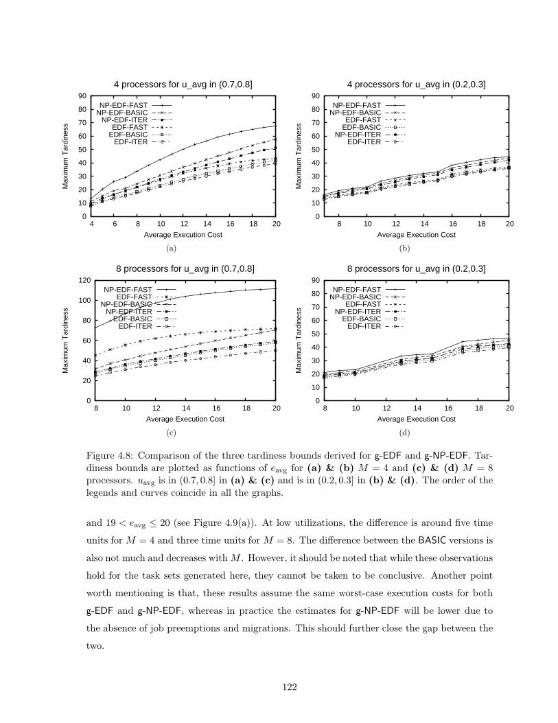
0

10

20

30

40

50

60

70

80

90

4 6 8 10 12 14 16 18 20

Max

imum

Tar

dine

ss

Average Execution Cost

4 processors for u_avg in (0.7,0.8]

NP-EDF-FASTNP-EDF-BASIC

NP-EDF-ITEREDF-FAST

EDF-BASICEDF-ITER

(a)

0

10

20

30

40

50

60

70

80

90

8 10 12 14 16 18 20

Max

imum

Tar

dine

ss




EDF-FASTEDF-BASIC

NP-EDF-ITEREDF-ITER

(b)

0

20

40

60

80

100

120

8 10 12 14 16 18 20

Max

imum

Tar

dine

ss



NP-EDF-FASTEDF-FAST

NP-EDF-BASICNP-EDF-ITER

EDF-BASICEDF-ITER

(c)

0

10

20

30

40

50

60

70

80

90

8 10 12 14 16 18 20

Max

imum

Tar

dine

ss




EDF-FASTNP-EDF-ITER

EDF-BASICEDF-ITER

(d)

Figure 4.8: Comparison of the three tardiness bounds derived for g-EDF and g-NP-EDF. Tar-diness bounds are plotted as functions of eavg for (a) & (b) M = 4 and (c) & (d) M = 8processors. uavg is in (0.7, 0.8] in (a) & (c) and is in (0.2, 0.3] in (b) & (d). The order of thelegends and curves coincide in all the graphs.

and 19 < eavg ≤ 20 (see Figure 4.9(a)). At low utilizations, the difference is around five time

units for M = 4 and three time units for M = 8. The difference between the BASIC versions is

also not much and decreases with M . However, it should be noted that while these observations

hold for the task sets generated here, they cannot be taken to be conclusive. Another point

worth mentioning is that, these results assume the same worst-case execution costs for both

g-EDF and g-NP-EDF, whereas in practice the estimates for g-NP-EDF will be lower due to

the absence of job preemptions and migrations. This should further close the gap between the

two.

122

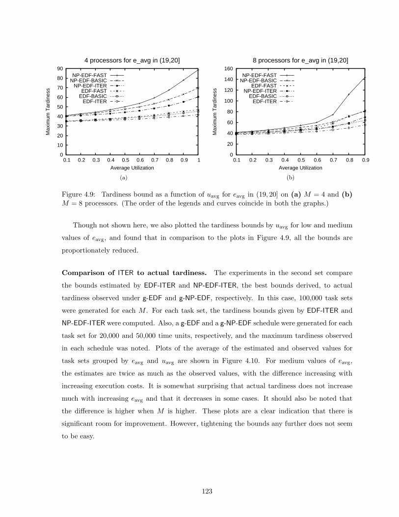
0

10

20

30

40

50

60

70

80

90

0.1 0.2 0.3 0.4 0.5 0.6 0.7 0.8 0.9 1

Max

imum

Tar

dine

ss

Average Utilization

4 processors for e_avg in (19,20]


NP-EDF-ITEREDF-FAST

EDF-BASICEDF-ITER

(a)

0

20

40

60

80

100

120

140

160

0.1 0.2 0.3 0.4 0.5 0.6 0.7 0.8 0.9

Max

imum

Tar

dine

ss

Average Utilization

8 processors for e_avg in (19,20]


EDF-FASTNP-EDF-ITER

EDF-BASICEDF-ITER

(b)

Figure 4.9: Tardiness bound as a function of uavg for eavg in (19, 20] on (a) M = 4 and (b)M = 8 processors. (The order of the legends and curves coincide in both the graphs.)

Though not shown here, we also plotted the tardiness bounds by uavg for low and medium

values of eavg, and found that in comparison to the plots in Figure 4.9, all the bounds are

proportionately reduced.

Comparison of ITER to actual tardiness. The experiments in the second set compare

the bounds estimated by EDF-ITER and NP-EDF-ITER, the best bounds derived, to actual

tardiness observed under g-EDF and g-NP-EDF, respectively. In this case, 100,000 task sets

were generated for each M . For each task set, the tardiness bounds given by EDF-ITER and

NP-EDF-ITER were computed. Also, a g-EDF and a g-NP-EDF schedule were generated for each

task set for 20,000 and 50,000 time units, respectively, and the maximum tardiness observed

in each schedule was noted. Plots of the average of the estimated and observed values for

task sets grouped by eavg and uavg are shown in Figure 4.10. For medium values of eavg,

the estimates are twice as much as the observed values, with the difference increasing with

increasing execution costs. It is somewhat surprising that actual tardiness does not increase

much with increasing eavg and that it decreases in some cases. It should also be noted that

the difference is higher when M is higher. These plots are a clear indication that there is

significant room for improvement. However, tightening the bounds any further does not seem

to be easy.

123

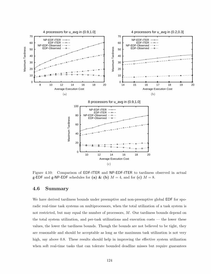
0

10

20

30

40

50

60

70

8 10 12 14 16 18 20

Max

imum

Tar

dine

ss



NP-EDF-ITEREDF-ITER

NP-EDF-ObservedEDF-Observed

(a)

0

10

20

30

40

50

60

70

14 15 16 17 18 19 20

Max

imum

Tar

dine

ss



NP-EDF-ITEREDF-ITER


(b)

0

20

40

60

80

100

10 12 14 16 18 20

Max

imum

Tar

dine

ss



NP-EDF-ITEREDF-ITER


(c)

Figure 4.10: Comparison of EDF-ITER and NP-EDF-ITER to tardiness observed in actualg-EDF and g-NP-EDF schedules for (a) & (b) M = 4, and for (c) M = 8.

4.6 Summary

We have derived tardiness bounds under preemptive and non-preemptive global EDF for spo-

radic real-time task systems on multiprocessors, when the total utilization of a task system is

not restricted, but may equal the number of processors, M . Our tardiness bounds depend on

the total system utilization, and per-task utilizations and execution costs — the lower these

values, the lower the tardiness bounds. Though the bounds are not believed to be tight, they

are reasonable and should be acceptable as long as the maximum task utilization is not very

high, say above 0.8. These results should help in improving the effective system utilization

when soft real-time tasks that can tolerate bounded deadline misses but require guarantees

124

on the long-run fraction of the processing time allocated are multiplexed on a multiprocessor.

Improving the accuracy of the bounds remains a challenging open problem.

Our task model can alternatively be viewed as one in which the relative deadline of each

task is greater than its period by an amount that is the same for all tasks and is dependent

on the parameters of the task system. Our conditions that check if a tardiness bound can be

guaranteed can then be used as schedulability tests for such task systems. While it is possible

to extend the EDF schedulability tests derived in prior research discussed in Section 4.1 to

task systems with relative deadlines greater than periods, it does not seem likely that such

extensions would allow total utilization to equal M even when per-task utilizations are low

and relative deadlines are large.

Apart from not being tight, another limitation of our result is that the tardiness bound that

can be guaranteed to each task is fixed and is dependent on task parameters. Guaranteeing

arbitrary and different tardiness bounds to different tasks is another challenging problem

towards which we have taken some steps in later work [52].

125

Chapter 5

EDF-fm: A Restricted-Migration Algorithm

for Soft Real-Time Systems1

In the previous chapter, we showed that on M ≥ 2 processors, preemptive and non-preemptive

global EDF can guarantee bounded tardiness to every sporadic task system τ with Usum(τ) ≤M . We also explained that since run-time overheads are lower under global EDF than under

known optimal algorithms, effective system utilization can be improved by scheduling soft

real-time systems under global EDF. However, task migrations under global EDF are still

unrestricted, which may be unappealing for some systems, but if migrations are forbidden

entirely, then bounded tardiness cannot be guaranteed. In this chapter, we address the issue

of finding an acceptable middle ground.

Our contributions are twofold. First, we present an algorithm called EDF-fm, which treads

a middle path between full-migration and no-migration algorithms, by restricting, but not

eliminating, task migrations, and derive a tardiness bound that can be guaranteed under it.

The tardiness bound derived can be computed in O(N) time, where N is the number of tasks.

Though our algorithm adheres to the conditions of the middle entry of Table 1.1 (restricted

migration, restricted dynamic priorities), the degree of migration that is needed is in fact lower

than that suggested by that entry: under EDF-fm, only up to M − 1 tasks, where M is the

number of processors, ever migrate, and those that do, do so only between jobs and only

between two processors. As noted in [42], migrations between jobs should not be much of a

concern for tasks for which little state is carried over from one job to the next.

1Contents of this chapter previously appeared in preliminary form in the following paper:[10] J. Anderson, V. Bud, and U. Devi. An EDF-based scheduling algorithm for multiprocessor soft real-timesystems. In Proceedings of the 17th Euromicro Conference on Real-Time Systems, pages 199–208, July 2005.

The maximum tardiness that any task may experience under EDF-fm is dependent on the

per-task utilization cap assumed—the lower the cap, the lower the tardiness threshold. Even

with a cap as high as 0.5 (half of the capacity of one processor), bounded tardiness can be

guaranteed for all the task systems. (In contrast, if α = 0.5 in the middle entry of Table 1.1,

then approximately 50% of the system’s overall capacity may be lost.) The percentage of task

systems for which bounded tardiness can be guaranteed decreases with the per-task utilization

cap and the number of processors. In our simulation experiments, we found that on sixteen

(resp., four) processors, bounded tardiness could be guaranteed to roughly 50% (resp., 75%)

and 75% (resp., 95%) of the task sets when umax = 1.0 and umax = 0.8, respectively. Hence,

our algorithm should enable a wide range of soft real-time applications to be scheduled in

practice with no constraints on total utilization. In addition, when a job misses its deadline,

we do not require a commensurate delay in the release of the next job of the same task. As a

result, each task’s required processor share is maintained over the long term.

As a second contribution, we propose several heuristics for assigning to processors those

tasks that do not migrate under EDF-fm, and, through extensive simulations, evaluate the

efficacy of these heuristics in lowering the tardiness bound that can be guaranteed. We also

present a simulation-based evaluation of the accuracy of the tardiness bound under the heuristic

identified to be the best. Finally, we provide a set of iterative formulas, which may potentially

require exponential time, for computing a tardiness bound that is less pessimistic than the

O(N)-time bound referred to earlier, and evaluate its accuracy through simulations.

The rest of this chapter is organized as follows. In Section 5.1, Algorithm EDF-fm is

presented and a tardiness bound under it that can be computed in O(N) time is derived.

Techniques and heuristics that can be used to reduce tardiness observed in practice, and

exponential-time iterative formulas for computing more accurate tardiness bounds, as de-

scribed above, are presented in Section 5.2. Then, in Section 5.3, a simulation-based evaluation

of our basic algorithm and proposed heuristics is presented, and the accuracy of the tardiness

bound derived is assessed. Section 5.4 concludes.

5.1 Algorithm EDF-fm

In this section, we present Algorithm EDF-fm (fm denotes that each task is either fixed or

migrating), an EDF-based multiprocessor scheduling algorithm for soft real-time sporadic task

systems. EDF-fm requires no restrictions on total system utilization and guarantees bounded

127

tardiness for task systems in which each task is light. Because a light task can consume up to

half the capacity of a single processor, we do not expect this limitation to be too restrictive

in practice. Further, at most M − 1 tasks need to be able to migrate, and each such task

migrates between two processors and at job boundaries only. This has the benefit of lowering

the number of tasks whose states need to be stored on any given processor and the number

of processors on which each task’s state needs to be stored. Also, the run-time context and

working set of a job, which can be expected to be larger than that of a task, need not be

transferred between processors.

EDF-fm consists of two phases: an assignment phase and an execution phase. The as-

signment phase executes offline and consists of sequentially assigning each task to one or two

processors. In the execution phase, jobs are scheduled for execution at run-time such that over

reasonable intervals (as explained later), each task executes at a rate that is commensurate

with its utilization. The two phases are explained in detail below. The following notation shall

be used.

si,jdef=

Percentage of Pj ’s processing capacity (expressed as a fraction)allocated to τi, 1 ≤ i ≤ N, 1 ≤ j ≤ M . (τi,j is said to have a shareof si,j on Pj .)

(5.1)

fi,jdef=

si,j

ui, the fraction of τi’s total workload that Pj can handle, 1 ≤

i ≤ N, 1 ≤ j ≤ M .(5.2)

ρidef=

Maximum percentage of Pi’s processing capacity (expressed as afraction) that can be allocated to tasks in τ , 1 ≤ i ≤ N . (Inother words, the sum of all shares assigned to tasks on Pi may notexceed ρi.)

5.1.1 Assignment Phase

The assignment phase assigns tasks to processors, with each task assigned to either one or two

processors. Tasks assigned to two processors are called migrating tasks, while those assigned to

only one processor are called fixed or non-migrating tasks. A fixed task τi is assigned a share,

si,j, equal to its utilization ui on the only processor Pj to which it is assigned. A migrating

task has shares on both processors to which it is assigned. The sum of its shares equals its

utilization. The assignment phase of EDF-fm also ensures that at most two migrating tasks

are assigned to each processor, and that on each Pi, the sum of allocations to all tasks does

not exceed a fraction ρi ≤ 1 of Pi’s processing capacity. (Since tardiness can be lowered by

lowering ρi, a value less than one may sometimes by desirable.)

128

global varu : array [1..N ] of rational

assigned task utilizations;ρ: array [1..M ] of rational

assigned processor capacities;s : array [1..N ] of array [1..M ]

of rational initially 0.0;p : array [1..N ] of array [1..2]

of 0..M initially 0;m: array [1..M ] of array [1..2]

of 0..N initially 0;f : array [1..M ] of array [1..N ]

of 0..N initially 0

Algorithm Assign-Tasks()

local var� identifier for current processor

proc : 1..M initially 1;� identifier for current task

task : 1..N ;� unassigned utilization on proc

AvailUtil : rational;

� indices of the migrating and fixed tasks� on current processor; mt and ft� are indices into m[proc] and f [proc]

mt , ft : integer initially 0

1 AvailUtil := ρ[1];2 for task := 1 to N do3 if AvailUtil ≥ u[task ] then4 s[task ][proc] := u[task ];5 AvailUtil := AvailUtil − u[task ];6 ft := ft + 1;7 p[task ][1] := proc;8 f [proc][ft ] := task

else9 if AvailUtil > 0 then

10 s[task ][proc] := AvailUtil ;11 mt := mt + 1;12 m[proc][mt ] := task ;13 p[task ][1] := proc;14 p[task ][2] := proc + 1;15 mt , ft := 1, 0;16 m[proc + 1][mt ] := task

else17 mt , ft := 0, 1;18 p[task ][1] := proc + 1;19 f [proc + 1][ft ] := task

fi20 proc := proc + 1;21 s[task ][proc] :=

u[task ] − s[task ][proc − 1];22 AvailUtil := ρ[proc] − s[task ][proc]

fiod

Figure 5.1: Algorithm Assign-Tasks.

In Figure 5.1, pseudo-code is given for a task-assignment algorithm, denoted Assign-

Tasks, that satisfies the following properties for every task system τ with umax(τ) ≤ min1≤ı≤N ρi

and Usum(τ) ≤∑Mi=1 ρi.

(P1) Each task is assigned shares on at most two processors. A task’s total share equals its

utilization.

(P2) Each processor is assigned at most two migrating tasks and may be assigned any number

of fixed tasks.

(P3) The sum of the shares allocated to all the tasks on Processor Pi is at most ρi.

In this pseudo-code, the ith element u[i] of the global array u represents the utilization ui

of task τi, s[i][j] denotes si,j (as defined in (5.1)), the ith element of array p, which is array p[i],

129

contains the processor(s) to which task i is assigned; arrays m[i] and f [i] denote the migrating

tasks and fixed tasks assigned to Processor i, respectively. Note that p[i] and m[i] are each

vectors of size two.

Assign-Tasks assigns tasks in sequence to processors, starting from the first processor.

Tasks and processors are both considered sequentially. Local variables proc and task denote

the current processor and task, respectively. Tasks are assigned to proc as long as the upper

limit, ρproc , on the processing capacity of proc is not exhausted. If the current task task cannot

receive its full share of utask from proc, then part of the processing capacity that it requires

is allocated on the next processor, proc + 1, such that the sum of the shares allocated to task

on the two processors equals utask. Note that if umax ≤ ρi, for all i, such an assignment is

possible for any task. It is easy to see that if Usum ≤∑Mi=1 ρi also holds, then assigning tasks

to processors following this simple approach satisfies (P1)–(P3).

ÅÆÇÈÉÊÊÇÆËÌ

ÍÎÏÌÐÎÑÒ

ÍÓÏÌÐÎÑÒ

ÍÔÏÌÐÌÕÒ

ÅÆÇÈÉÊÊÇÆËÕ

ÍÌÏÕÐÔÑÒ

ÍÑÏÕÐÌÕÒÍÕÏÕÐÖÑÒ

ÅÆÇÈÉÊÊÇÆËÑ

Í×ÏÑÐÑÖ

ÍÖÏÑÐÑÖ

ÍØÏÑÐÕÕÒÍÎÏÑÐÕÑÒ

ÍÌÏÑÐÕÑÒ

Figure 5.2: Task assignment on three processors forthe task set in Example 5.1 using Algorithm Assign-

Tasks.

Example 5.1. Consider a task set

τ with the following nine tasks:

τ1(5, 20), τ2(3, 10), τ3(1, 2), τ4(2, 5),

τ5(2, 5), τ6(1, 10), τ7(2, 5), τ8(7, 20),

and τ9(3, 10). The total utilization of

this task set is three. A share as-

signment produced by Assign-Tasks

when ρ1 = ρ2 = ρ3 = 1.0 is shown in

Figure 5.2. In this assignment, τ3 and

τ7 are migrating tasks; the remaining

tasks are fixed. τ3 has a share of 920

on processor P1 and a share of 120 on

processor P2, while τ7 has shares of 120 and 7

20 on processors P2 and P3, respectively.

5.1.2 Execution Phase

Having devised a way of assigning tasks to processors, the next step is to devise an online

scheduling algorithm that is easy to analyze and can ensure bounded tardiness. For a fixed

task, we merely need to decide when to schedule each of its jobs on its (only) assigned processor.

For a migrating task, we must decide both when and where its jobs should execute. Before

describing our scheduling algorithm, we discuss some considerations that led to its design.

130

In order to analyze a scheduling algorithm and for the algorithm to guarantee bounded

tardiness, it should be possible to bound the total demand for execution time by all tasks on

each processor over well-defined time intervals. We first argue that bounding total demand

may not be possible if the jobs of migrating tasks are allowed to miss their deadlines.

Recall that a deadline miss of a job does not lead to a postponement of the release times of

subsequent jobs of the same task. Furthermore, no two jobs of a task may execute in parallel.

Hence, the tardiness of a job of a migrating task executing on one processor can postpone the

execution of its successor job, which may otherwise execute in a timely manner on a second

processor. In the worst case, the second processor may be forced to idle. The tardiness of the

second job may also impact the timeliness of fixed tasks and other migrating tasks assigned

to the same processor, which in turn may lead to deadline misses of both fixed and migrating

tasks on other processors or unnecessary idling on other processors.

As a result, a set of dependencies is created among the jobs of migrating tasks, resulting

in an intricate linkage among processors that complicates scheduling analysis. It is unclear

how per-processor demand can be precisely bounded when activities on different processors

become interlinked.

Let us look at a concrete example that reveals this linkage among processors. Consider the

task set τ , introduced earlier, with task assignments and processor shares shown in Figure 5.2.

For simplicity, assume that the execution of the jobs of a migrating task alternate between the

two processors to which the task is assigned. τ3 releases its first job on P1, while τ7 releases its

first job on P3. (We are assuming such a naıve assignment pattern to illustrate the processor

linkage using a short segment of a real schedule. Such a linkage occurs even with an intelligent

job-assignment pattern if migrating tasks miss their deadlines.) A complete schedule up to

time 27, with the jobs assigned to each processor scheduled using EDF, is shown in Figure 5.3.

In Figure 5.3, the sixth job of the migrating task τ3 misses its deadline (at time 12) on P2

and completes executing at time 14. This prevents the next job of τ3 released on P1 from being

scheduled until time 14 and it misses its deadline. Because job releases are not postponed due

to deadline misses, the seventh job of τ3 is released at time 12 and has a deadline at time 14.

The missed deadline of the migrating task τ3 impacts the execution of the fixed tasks also

on P2. (It may seem that τ3’s misses can be avoided by determining processor assignments for

its jobs dynamically. However, a reasonable strategy that is not convoluted does not appear

to be possible.) The deadline misses of the fixed tasks τ4, τ5, and τ6 cause the migrating task

τ7 to miss a deadline on P2. In particular, the fourth job of τ7 misses its deadline, which in

131

τ3(1,2)

τ2(3,10)

τ1(5,20)

τ4(2,5) Ù ÙÙ ÙÙ ÙÙ Ù

Ú ÚÚ ÚÚ ÚÚ ÚÛ ÛÛ ÛÛ ÛÛ ÛÜ ÜÜ ÜÜ ÜÜ Ü

tard

Ý ÝÝ ÝÝ ÝÞ ÞÞ ÞÞ Þß ßß ßß ßà àà àà àτ5

(2,5)

τ6(1,10)

τ7(2,5)

τ8(7,20)

τ9(3,10)

P3

P2

P1

á áá áá áâ ââ ââ â ã ãã ãã ãä ää ää ä

å åå åå åæ ææ ææ æ ç çç çç çè èè èè è é é éé é éé é é

ê ê êê ê êê ê êë ë ëë ë ëë ë ëì ìì ìì ìí í íí í íí í íí í í

î îî îî îî îï ï ïï ï ïï ï ïï ï ïð ð ðð ð ðð ð ðð ð ð

ñ ñ ññ ñ ññ ñ ñò òò òò òó ó óó ó óó ó óô ô ôô ô ôô ô ô

õ õ õõ õ õõ õ õõ õ õö öö öö öö ö÷ ÷ ÷÷ ÷ ÷÷ ÷ ÷ø ø øø ø øø ø ø

ù ùù ùù ùú úú úú ú û ûû ûû ûü üü üü ü ý ý ýý ý ýý ý ý

þ þ þþ þ þþ þ þÿ ÿ ÿÿ ÿ ÿÿ ÿ ÿ� ��

� ��

� � ��

� ��

� � ��

� � ��

tard tard

tard

tard

tard

tard

tard

tard

0 2 4 6 8 10 12 14 16 18 20 22 24 26

time

tard tard tard

tard

tard

Figure 5.3: Illustration of processor linkage.

turn reduces the interval over which the fifth job of the same task can execute on P3. Note

that jobs τ9,3 and τ8,2 execute before τ7,5, as this job is forced to wait for its predecessor to

complete executing on P2. Thus, a nontrivial linkage is established among the processors that

impacts system tardiness.

Per-processor scheduling rules. EDF-fm eliminates this linkage among processors by en-

suring that migrating tasks do not miss their deadlines. Jobs of migrating tasks are assigned

to processors using static rules that are independent of run-time dynamics. The jobs assigned

132

...

...

...

� ��

...

� ��

... ...

��

...

higher priority

higher priority

higher priority

lowerpriority

lowerpriority

lowerpriority

�� . . .

...

SPSSPSSPS

SPS

EDFEDF EDF EDF EDF EDF

L E G E N D

�� !"#$��%&'(�!&)'*�!+��)#$�) #$,-.!�!&/01(&"(&!2./3� 45�(6�� 274�4�"89"*�"8�� !��6�� 274�4�"89"*�"8%&'(�!&)'!��

:;

:< := :>

1("/��"(?

@A- @AB @ACDA- DAB

DA$@A$

Figure 5.4: Schematic representation of EDF-fm in the execution phase.

to a processor are scheduled independently of other processors, and on each processor, migrat-

ing tasks are statically prioritized over fixed tasks. Jobs within each task class are scheduled

using EDF, which is optimal on uniprocessors. A schematic representation of EDF-fm in the

execution phase is shown in Figure 5.4. This priority scheme, together with the restriction that

migrating tasks have utilizations at most 1/2, and the task assignment property (from (P2))

that there are at most two migrating tasks per processor, ensures that migrating tasks never

miss their deadlines. Therefore, the jobs of migrating tasks executing on different processors

do not impact one another, and each processor can be analyzed independently. Thus, the

multiprocessor scheduling analysis problem at hand is transformed into a simpler uniprocessor

one.

In the description of EDF-fm, we are left with defining rules that map the jobs of migrat-

ing tasks to processors. A naıve assignment of the jobs of a migrating task to its processors

can cause an over-utilization on one of its assigned processors. EDF-fm follows a job assign-

ment pattern that prevents over-utilization in the long run by ensuring that over well-defined

time intervals (explained later), on each processor, the demand due to a migrating task is in

accordance with its allocated share on that processor.

For example, consider the migrating task τ7(2, 5) in the example above. τ7 has a share of

s7,2 = 120 on P2 and s7,3 = 7

20 on P3. Also, f7,2 =s7,2

u7= 1

8 and f7,3 =s7,3

u7= 7

8 , which imply

133

T7,2 T7,7 T7,12 T7,13 T7,14 T7,15

T7,16

T7,4 T7,5T7,1 T7,6

T7,8

T7,9 T7,10 T7,11T7,3

to P2

Jobs assigned

Jobs assignedto P

3

0 5 10 15 20 25 30 35 40 45 50 55 60 65 70 75 80

time

Figure 5.5: Assignment of periodically released jobs of migrating task τ7 to processors P2 andP3.

that P2 and P3 should be capable of executing 18 and 7

8 of the workload of τ7, respectively. Our

goal is to devise a job assignment pattern that would ensure that, in the long run, the fraction

of a migrating task τi’s workload executed on Pj is close to fi,j, and at any time, deviation

from this ideal is minimized. One such job assignment pattern for τ7 over interval [0, 80) is

shown in Figure 5.5. Assuming that τ7 is a synchronous, periodic task,2 the pattern in [0, 40)

would repeat every 40 time units.

In the job assignment of Figure 5.5, exactly one job out of every eight consecutive jobs of τ7

released in the interval [5k, 5(k +8)), where k ≥ 0, is assigned to P2. Because e7 = 2, τ7 places

a demand for two units of time, i.e., 1/20th of P2, in [5k, 5(k + 8)). Because τ7 is allocated a

share of s7,2 = 1/20 on P2, this job assignment pattern ensures that in the long run τ7 does

not overload P2. However, the demand due to τ7 on P2 over short intervals may exceed or fall

below the share allocated to it. For instance, under the above job assignment, τ7 requires two

units of time, i.e., 2/5 of P2 in the interval [40k + 35, 40(k + 1)), and zero time units in the

interval [40k, 40k + 35). Similarly, exactly seven out of every eight consecutive jobs of τ7 are

assigned to P3. Thus, τ7 requires 14 units of time, or 7/20 of the time, in [5k, 5(k + 8)), and

the share allocated to it matches this need. However, as with P2, the demand due to τ7 on P3

over shorter intervals may deviate from its long-term share.

A job assignment pattern like the one described above can ensure that, over the long term,

the demand of each migrating task on each processor is in accordance with the share allocated

to it. However, as explained above, such an assignment pattern can result in a migrating

task overloading a processor over short time intervals, leading to deadline misses for fixed

tasks. Nevertheless, because a deadline miss of a job does not delay the next job release of the

same task, this scheme also ensures, over the long term, that each fixed task executes at its

prescribed rate (given by its utilization). Later in this section, we show that the amount by

2The first job of a synchronous, periodic task is released at time 0.

134

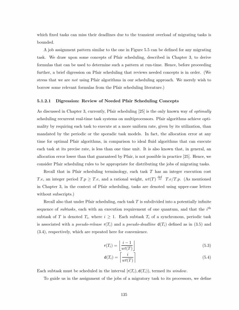
which fixed tasks can miss their deadlines due to the transient overload of migrating tasks is

bounded.

A job assignment pattern similar to the one in Figure 5.5 can be defined for any migrating

task. We draw upon some concepts of Pfair scheduling, described in Chapter 3, to derive

formulas that can be used to determine such a pattern at run-time. Hence, before proceeding

further, a brief digression on Pfair scheduling that reviews needed concepts is in order. (We

stress that we are not using Pfair algorithms in our scheduling approach. We merely wish to

borrow some relevant formulas from the Pfair scheduling literature.)

5.1.2.1 Digression: Review of Needed Pfair Scheduling Concepts

As discussed in Chapter 3, currently, Pfair scheduling [25] is the only known way of optimally

scheduling recurrent real-time task systems on multiprocessors. Pfair algorithms achieve opti-

mality by requiring each task to execute at a more uniform rate, given by its utilization, than

mandated by the periodic or the sporadic task models. In fact, the allocation error at any

time for optimal Pfair algorithms, in comparison to ideal fluid algorithms that can execute

each task at its precise rate, is less than one time unit. It is also known that, in general, an

allocation error lower than that guaranteed by Pfair, is not possible in practice [25]. Hence, we

consider Pfair scheduling rules to be appropriate for distributing the jobs of migrating tasks.

Recall that in Pfair scheduling terminology, each task T has an integer execution cost

T.e, an integer period T.p ≥ T.e, and a rational weight, wt(T )def= T.e/T.p. (As mentioned

in Chapter 3, in the context of Pfair scheduling, tasks are denoted using upper-case letters

without subscripts.)

Recall also that under Pfair scheduling, each task T is subdivided into a potentially infinite

sequence of subtasks, each with an execution requirement of one quantum, and that the ith

subtask of T is denoted Ti, where i ≥ 1. Each subtask Ti of a synchronous, periodic task

is associated with a pseudo-release r(Ti) and a pseudo-deadline d(Ti) defined as in (3.5) and

(3.4), respectively, which are repeated here for convenience.

r(Ti) =

⌊

i − 1

wt(T )

⌋

(5.3)

d(Ti) =

⌈

i

wt(T )

⌉

(5.4)

Each subtask must be scheduled in the interval [r(Ti), d(Ti)), termed its window .

To guide us in the assignment of the jobs of a migratory task to its processors, we define

135

the notion of a complementary task .

Definition 5.1: Task T is said to be complementary to U iff wt(U) = 1 − wt(T ).

T1

T2

T3

1 2 3 4 5 760

1 2 3 4 5 760

time

slot

U1

U3

U4X

X

XT (3/7)

X

X

U (4/7)

U2

X

X

Figure 5.6: A partial complementary Pfair schedule for a pairof complementary tasks, T and U , on one processor. The slotin which a subtask is scheduled is indicated by an “X.” Everysubtask of U is scheduled in the first slot of its window, whileevery subtask of T is scheduled in the last slot.

Tasks T and U shown in Fig-

ure 5.6 are complementary to

one another. A partial Pfair

schedule for these two tasks

on one processor, in which the

subtasks of T are always sched-

uled in the last slots of their

windows and those of U in

the first slots, is also shown.

We call such a schedule a

complementary schedule. By

Lemma 5.1 below such a sched-

ule is always possible for two

complementary periodic tasks.

Lemma 5.1 For any two syn-

chronous, periodic tasks T and U that are complementary, a schedule in which every subtask

of T is scheduled in the first slot of its window and every subtask of U in its last slot, or vice

versa, is feasible on one processor.

Proof: To show that the lemma holds, it suffices to show the following: for all t, if r(Ti) = t

holds for some i, then there does not exist a j such that d(Uj) = t+1. (Here t is a non-negative

integer, and i and j are positive integers.) The contrapositive of the above assertion would

then imply that for all t, if there exists a j such that d(Uj) = t + 1, then there dose not exist

an i for which r(Ti) = t. Hence, a schedule as described in the statement of the lemma would

be feasible.

By (5.3), r(Ti) = t implies that

⌊

i − 1wt(T )

⌋

= t holds. Therefore,

i − 1

wt(T )≥ t

⇒ i ≥ t · wt(T ) + 1

136

⇒ t − i ≤ t(1 − wt(T )) − 1

⇒ t − i + 1

1 − wt(T )≤ t. (5.5)

Furthermore, by

⌊

i − 1wt(T )

⌋

= t, we also have the following.

i − 1

wt(T )< t + 1

⇒ i − 1 < wt(T ) + t · wt(T )

⇒ t − i + 1 + wt(T ) > t(1 − wt(T ))

⇒ t − i + 1 + wt(T )

1 − wt(T )> t

⇒ t − i + 1 + wt(T )

1 − wt(T )+

1 − wt(T )

1 − wt(T )> t +

1 − wt(T )

1 − wt(T )

⇒ t − i + 2

1 − wt(T )> t + 1 (5.6)

By (5.5) and (5.6), it follows that there does not exist an integer j for which

⌈

j1 − wt(T )

⌉

= t+1

holds. By Definition 5.1, wt(U) = 1 − wt(T ). Therefore, by (5.4), it follows that there does

not exist a subtask Uj such that d(Uj) = t + 1 holds. �

With the above introduction to Pfair scheduling, we are now ready to present the details

of distributing the jobs of a migrating task between its processors.

5.1.2.2 Assignment Rules for Jobs of Migrating Tasks

Let τi be any migrating periodic task (we later relax the assumption that τi is periodic)

that is assigned shares si,j and si,j+1 on processors Pj and Pj+1, respectively. (Recall that

every migrating task is assigned shares on two consecutive processors by Assign-Tasks.) As

explained earlier, fi,j and fi,j+1 (given by (5.2)) denote the fraction of the workload (i.e., the

total execution requirement) of T that should be executed on Pj and Pj+1, respectively, in the

long run. By (P1), the total share allocated to τi on Pj and Pj+1 is ui. Hence, by (5.2), it

follows that

fi,j + fi,j+1 = 1. (5.7)

Assuming that the execution cost and period of every task are rational numbers (which can

be expressed as a ratio of two integers), ui, si,j, and hence, fi,j and fi,j+1 are also rational

numbers. Let fi,j =xi,j

yi, where xi,j and yi are positive integers that are relatively prime.

137

Then, by (5.7), it follows that fi,j+1 =yi−xi,j

yi. Therefore, one way of distributing the workload

of τi between Pj and Pj+1 that is commensurate with the shares of τi on the two processors

would be to assign xi,j out of every yi jobs to Pj and the remaining jobs to Pj+1.

Rather than arbitrarily choosing the xi,j jobs to assign to Pj , we borrow from the afore-

mentioned concepts of Pfair scheduling to guide in the distribution of jobs. For illustration,

consider a migrating task τi with utilization 38 that is assigned shares si,j = 1

5 and si,j+1 = 740

on Pj and Pj+1, respectively. Hence, fi,j = 815 and fi,j+1 = 7

15 hold. Therefore, one way of

distributing τi’s jobs would be to assign the first eight of jobs 15k + 1, · · · , (15k + 15), for all

k ≥ 0, to Pj , and the remaining jobs to Pj+1. Though such a strategy is reasonable (and

perhaps among the best) for the example in Figure 5.5, the distribution may be significantly

uneven over short durations for some task systems, such as the present example, and the tran-

sient overload that ensues may be quite excessive. As we shall see, a more even distribution

of jobs can be obtained by applying Pfair rules.

If we let two fictitious periodic Pfair tasks V and W correspond to processors Pj and Pj+1,

respectively, let fi,j and fi,j+1 denote their weights, and let a quantum span pi time units,

then the following analogy can be made between the jobs of the migrating task τi and the

subtasks of the fictitious tasks V and W . First, slot s can be associated with job s + 1 in that

slot s represents the interval in which the (s + 1)st job of τi, which is released at the beginning

of that slot, needs to be scheduled. (Recall that slots are numbered starting from 0.) This is

illustrated in Figure 5.7(a), which depicts the layouts of subtasks in the first period of V and

W for the example mentioned above, and a complementary schedule for those subtasks on a

fictitious processor. Refer to “slots” and “jobs” marked beneath the time line. Continuing

with the analogy, subtask Vg represents the gth job assigned to Pj (of the jobs of τi); that is,

exactly one of the jobs that correspond to slots r(Vg), · · · , d(Vg) − 1 should be assigned as the

gth job of Pj . Similarly, subtask Wh represents the hth job assigned to Pj+1. Finally, if subtask

Vg (resp., Wh) is scheduled in slot s (on a fictitious processor), then the (s + 1)st job of τi

should be assigned to Pj (resp., Pj+1). In other words, job s + 1 is assigned to the processor

that corresponds to the Pfair task that is scheduled in slot s + 1. Referring to Figure 5.7(a),

since subtask V1 is scheduled in slot 0, the first job of τi is assigned to Pj . Similarly, since

subtasks of V are scheduled in slots 1, 3, 5, 7, 9, 11, and 13, jobs 2, 4, 6, 8, 10, 12, and 14 of

τi are assigned to Pj , and since subtasks of W are scheduled in slots 2, 4, 6, 8, 10, 12, and 14,

jobs 3, 5, 7, 9, 11, 13, and 15 of τi are assigned to Pj+1.

By Definition 5.1 and (5.7), Pfair tasks V and W are complementary. Therefore, by

138

~ ~

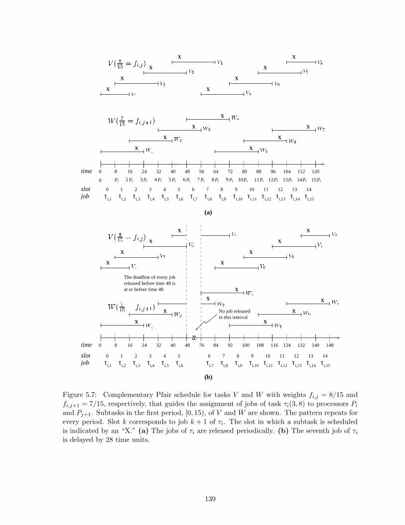
pi2 pi10 pi11 pi12 pi13 pi14 pi15

time

slotjob

6 7 8 9 10 11 12 13 14

τi,7 τi,8 τi,9 τi,10 τi,11 τi,12 τi,13 τi,14 τi,15

1 2 3 4 50

τi,1 τi,2 τi,3 τi,4 τi,5 τi,6

slotjob

pi

XX

0 8 24 32 40 48 76 84 100 108 116 124 14013216 92

X

X

X

X

X

X

X

148

No job releasedin this interval

The deadline of every jobreleased before time 48 isat or before time 48

0 8 24 32 40 48 56 64 80 88 96 104 120112

0

16 72

pi3 pi4 pi5 pi6 pi7 pi8 pi9

1 2 3 4 5 6 7 8 9 10 11 12 13 140

τi,1 τi,2 τi,3 τi,4 τi,5 τi,6 τi,7 τi,8 τi,9 τi,10 τi,11 τi,12 τi,13 τi,14 τi,15

X

X

X

X

X

X

X

X

X

X

X

X

X

time

(a)

(b)

X

X

X

X

X

X

X

X

E F GHI J KLMN O

P F QHI J KLMNRHO

STSU

SVSW

SXSY

SZS[

\T\U

\V\W

\X\Y

\Z

E F GHI J KLMN O

P F QHI J KLMNRHO

STSU

SVSW

SXSY

SZS[

\T\U

\V\W

\X\Y

\Z

Figure 5.7: Complementary Pfair schedule for tasks V and W with weights fi,j = 8/15 andfi,j+1 = 7/15, respectively, that guides the assignment of jobs of task τi(3, 8) to processors Pi

and Pj+1. Subtasks in the first period, [0, 15), of V and W are shown. The pattern repeats forevery period. Slot k corresponds to job k + 1 of τi. The slot in which a subtask is scheduledis indicated by an “X.” (a) The jobs of τi are released periodically. (b) The seventh job of τi

is delayed by 28 time units.

139

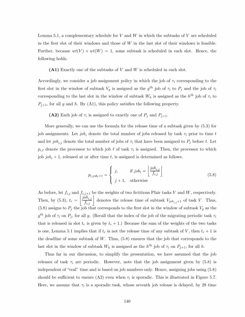
Lemma 5.1, a complementary schedule for V and W in which the subtasks of V are scheduled

in the first slot of their windows and those of W in the last slot of their windows is feasible.

Further, because wt(V ) + wt(W ) = 1, some subtask is scheduled in each slot. Hence, the

following holds.

(A1) Exactly one of the subtasks of V and W is scheduled in each slot.

Accordingly, we consider a job assignment policy in which the job of τi corresponding to the

first slot in the window of subtask Vg is assigned as the gth job of τi to Pj and the job of τi

corresponding to the last slot in the window of subtask Wh is assigned as the hth job of τi to

Pj+1, for all g and h. By (A1), this policy satisfies the following property.

(A2) Each job of τi is assigned to exactly one of Pj and Pj+1.

More generally, we can use the formula for the release time of a subtask given by (5.3) for

job assignments. Let jobi denote the total number of jobs released by task τi prior to time t

and let jobi,j denote the total number of jobs of τi that have been assigned to Pj before t. Let

pi,` denote the processor to which job ` of task τi is assigned. Then, the processor to which

job jobi + 1, released at or after time t, is assigned is determined as follows.

pi,jobi+1 =

j, if jobi =

⌊

jobi,j

fi,j

⌋

j + 1, otherwise

(5.8)

As before, let fi,j and fi,j+1 be the weights of two fictitious Pfair tasks V and W , respectively.

Then, by (5.3), tr =

⌊

jobi,j

fi,j

⌋

denotes the release time of subtask Vjobi,j+1 of task V . Thus,

(5.8) assigns to Pj the job that corresponds to the first slot in the window of subtask Vg as the

gth job of τi on Pj , for all g. (Recall that the index of the job of the migrating periodic task τi

that is released in slot tr is given by tr + 1.) Because the sum of the weights of the two tasks

is one, Lemma 5.1 implies that if tr is not the release time of any subtask of V , then tr + 1 is

the deadline of some subtask of W . Thus, (5.8) ensures that the job that corresponds to the

last slot in the window of subtask Wh is assigned as the hth job of τi on Pj+1, for all h.

Thus far in our discussion, to simplify the presentation, we have assumed that the job

releases of task τi are periodic. However, note that the job assignment given by (5.8) is

independent of “real” time and is based on job numbers only. Hence, assigning jobs using (5.8)

should be sufficient to ensure (A2) even when τi is sporadic. This is illustrated in Figure 5.7.

Here, we assume that τi is a sporadic task, whose seventh job release is delayed, by 28 time

140

units, to time 76 from time 48. As far as τi is concerned, the interval [48, 76) is “frozen” and

the job assignment resumes at time 76. As indicated in the figure, in any such interval in

which activity is suspended for a migrating task τi, no jobs of τi are released. Furthermore,

the deadlines of all jobs of τi released before the frozen interval fall at or before the beginning

of the interval.

We next prove a property that bounds from above the number of jobs of a migrating task

assigned to each of its processors by the job assignment rule given by (5.8).

Lemma 5.2 Let τi be a migrating task that is assigned to processors Pj and Pj+1. The number

of jobs out of any consecutive ` ≥ 0 jobs of τi that are assigned to Pj and Pj+1 is at most

d` · fi,je and d` · fi,j+1e, respectively.

Proof: We first prove the lemma for the number of jobs assigned to Pj . We begin by claiming

the following.

(J) Exactly d`0 · fi,je of the first `0 jobs of τi are assigned to Pj.

(J) holds trivially when `0 = 0. Therefore, assume `0 ≥ 1. Let q denote the total number of

jobs of the first `0 jobs of τi that are assigned to Pj . (By (5.8), the first job of τi is assigned

to Pj , hence, q ≥ 1 holds.) Then, there exists an `′ ≤ `0 such that job `′ of τi is the qth job of

τi assigned to Pj . Therefore, by (5.8),

`′ − 1 =

⌊

q − 1fi,j

⌋

(5.9)

holds. (Note that jobi of (5.8) denotes the number of jobs of τi that have already been

distributed, and hence, is equal to ` − 1 here. Similarly, jobi,j denotes the number of jobs

already assigned to to Pj , and so is equal to q − 1.) `, `′, and q denote job numbers or counts,

and hence are all non-negative integers. By (5.9), we have

q − 1

fi,j≥ `′−1 ⇒ q−1 ≥ (`′−1) ·fi,j ⇒ q > `′ ·fi,j (because fi,j < 1), (5.10)

andq − 1

fi,j< `′ ⇒ q − 1 < `′ · fi,j ⇒ q < `′ · fi,j + 1. (5.11)

Because q is an integer, by (5.10) and (5.11), we have

q = d`′ · fi,je. (5.12)

141

If `′ = `0 holds, then (J) follows from (5.12) and our definition of q. On the other hand, to

show that (J) holds when `′ < `0, we must show that q = dˆ· fi,je holds for all ˆ, where `′ < ˆ

≤ `0. (Note that ˆ is an integer.) By the definitions of q, `′, and `0, q of the first `′ jobs of

τi are assigned to Pj , and none of the jobs `′ + 1 through `0 is assigned to Pj . Therefore, by

(5.8), it follows that ˆ− 1 <

⌊

qfi,j

⌋

holds for all ˆ, where `′ < ˆ ≤ `0. (As before, because ˆ

is the index of the next job of τi to be distributed, jobi of (5.8) equals ˆ− 1. However, since

the number of jobs already assigned to Pj is q, jobi,j = q.) Thus, we have the following, for

all ˆ, where `′ < ˆ ≤ `0.

⌊

qfi,j

⌋

> ˆ− 1 ⇒⌊

qfi,j

⌋

≥ ˆ ⇒ q

fi,j≥ ˆ ⇒ q ≥ ˆ· fi,j ⇒ q ≥ dˆ· fi,je

(because q is an integer) (5.13)

By (5.12) and because ˆ> `′ holds, (5.13) implies that dˆ· fi,je = d`′ · fi,je = q.

To complete the proof for Pj , we show that at most d` · fi,je of any consecutive ` jobs of

τi are assigned to Pj . Let J represent jobs `0 + 1 to `0 + ` of τi, where `0 ≥ 0. Then, by

(J), exactly d`0 · fi,je of the first `0 jobs and d(`0 + `) · fi,je of the first `0 + ` jobs of τi are

assigned to Pj . Therefore, the number of jobs belonging to J that are assigned to Pj , denoted

Jobs(J , j), is given by

Jobs(J , j) = d(`0 + `) · fi,je − d`0 · fi,je ≤ d`0 · fi,je + d` · fi,je − d`0 · fi,je = d` · fi,je,

which proves the lemma for the number of jobs assigned to Pi. (The second step in the above

derivation follows from dx + ye ≤ dxe + dye.)Finally, we are left with proving the lemma for Pj+1. By the job assignment rule in (5.8),

every job of τi is assigned to exactly one of Pj and Pj+1. Therefore (J) implies that exactly

`0−d`0 · fi,je of the first `0 jobs of τi are assigned to Pj+1. Hence, the number of jobs belonging

to J that are assigned to Pj+1 is given by

Jobs(J , j + 1) = (`0 + `) − d(`0 + `) · fi,je − `0 + d`0 · fi,je

= ` − d(`0 + `) · fi,je + d`0 · fi,je

≤ ` − d`0 · fi,je − b` · fi,jc + d`0 · fi,je (because dx + ye ≥ dxe + byc)

= ` − b` · fi,jc

< ` − ` · fi,j + 1

142

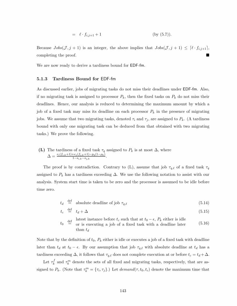
= ` · fi,j+1 + 1 (by (5.7)).

Because Jobs(J , j + 1) is an integer, the above implies that Jobs(J , j + 1) ≤ d` · fi,j+1e,completing the proof. �

We are now ready to derive a tardiness bound for EDF-fm.

5.1.3 Tardiness Bound for EDF-fm

As discussed earlier, jobs of migrating tasks do not miss their deadlines under EDF-fm. Also,

if no migrating task is assigned to processor Pk, then the fixed tasks on Pk do not miss their

deadlines. Hence, our analysis is reduced to determining the maximum amount by which a

job of a fixed task may miss its deadline on each processor Pk in the presence of migrating

jobs. We assume that two migrating tasks, denoted τi and τj, are assigned to Pk. (A tardiness

bound with only one migrating task can be deduced from that obtained with two migrating

tasks.) We prove the following.

(L) The tardiness of a fixed task τq assigned to Pk is at most ∆, where

∆ =ei(fi,k+1)+ej(fj,k+1)−pq(1−ρk)

1−si,k−sj,k.

The proof is by contradiction. Contrary to (L), assume that job τq,` of a fixed task τq

assigned to Pk has a tardiness exceeding ∆. We use the following notation to assist with our

analysis. System start time is taken to be zero and the processor is assumed to be idle before

time zero.

tddef= absolute deadline of job τq,` (5.14)

tcdef= td + ∆ (5.15)

t0def=

latest instance before tc such that at t0 − ε, Pk either is idleor is executing a job of a fixed task with a deadline laterthan td

(5.16)

Note that by the definition of t0, Pk either is idle or executes a job of a fixed task with deadline

later than td at t0 − ε. By our assumption that job τq,` with absolute deadline at td has a

tardiness exceeding ∆, it follows that τq,` does not complete execution at or before tc = td +∆.

Let τ fk and τm

k denote the sets of all fixed and migrating tasks, respectively, that are as-

signed to Pk. (Note that τmk = {τi, τj}.) Let demand(τ, t0, tc) denote the maximum time that

143

jobs of tasks in τ could execute in the interval [t0, tc) on Processor Pk (under the assump-

tion that τq,` does not complete executing at tc). We first determine demand(τmk , t0, tc) and

demand(τ fk , t0, tc).

By (5.16) and because migrating tasks have a higher priority than fixed tasks under EDF-

fm, jobs of τi and τj that are released before t0 and are assigned to Pk complete executing at

or before t0. Thus, every job of τi or τj that executes in [t0, tc) on Pk is released in [t0, tc).

Also, every job released in [t0, tc) and assigned to Pk places a demand for execution in [t0, tc).

The number of jobs of τi that are released in [t0, tc) is at most⌈

tc − t0pi

⌉

. By Lemma 5.2, at

most⌈

fi,k

⌈

tc − t0pi

⌉⌉

≤ fi,k

(

tc−t0pi

+ 1)

+ 1 of all the jobs of τi released in [t0, tc) are assigned

to Pk. Similarly, the number of jobs of τj that are assigned to Pk of all jobs of τi released in

[t0, tc) is at most fj,k

(

tc−t0pj

+ 1)

+ 1. Each job of τi executes for at most ei time units and

that of τj for ej time units. Therefore,

demand(τmk , t0, tc) ≤

(

fi,k

(

tc − t0pi

+ 1

)

+ 1

)

· ei +

(

fj,k

(

tc − t0pj

+ 1

)

+ 1

)

· ej

= si,k(tc − t0) + ei(fi,k + 1) + sj,k(tc − t0) + ej(fj,k + 1) (5.17)

(by (5.2) and simplification).

By (5.14)–(5.16), and our assumption that the tardiness of τq,` exceeds ∆, any job of a

fixed task that executes on Pk in [t0, tc) is released at or after t0 and has a deadline at or before

td. The number of such jobs of a fixed task τf is at most⌊

td − t0pf

⌋

. Therefore,

demand(τ fk , t0, tc) ≤

∑

τf∈τf

k

⌊

td − t0pf

⌋

· ef

≤ (td − t0)∑

τf∈τfk

ef

pf

≤ (td − t0)(ρk − si,k − sj,k) (by (P3)). (5.18)

By (5.17) and (5.18), we have the following.

demand(τ fk ∪ τm

k , t0, tc)

si,k(tc − t0) + ei(fi,k + 1) + sj,k(tc − t0) + ej(fj,k + 1) + (td − t0)(ρk − si,k − sj,k)

= (si,k + sj,k)(tc − t0) + (si,k + sj,k)(t0 − td) + ei(fi,k + 1) + ej(fj,k + 1) + (td − t0)(ρk)

= (si,k + sj,k)(tc − td) + ei(fi,k + 1) + ej(fj,k + 1) + ρk(td − t0)

144

Because τq,` does not complete executing by time tc, it follows that the total processor time

available in the interval [t0, tc) = tc − t0 < demand(τ fk ∪ τm

k , t0, tc), i.e.,

tc − t0 < (si,k + sj,k)(tc − td) + ei(fi,k + 1) + ej(fj,k + 1) + ρk(td − t0)

= (si,k + sj,k)(tc − td) + ei(fi,k + 1) + ej(fj,k + 1) + (td − t0)

−(1 − ρk)(td − t0)

⇒ tc − td < (si,k + sj,k)(tc − td) + ei(fi,k + 1) + ej(fj,k + 1) − (1 − ρk)(td − t0)

≤ (si,k + sj,k)(tc − td) + ei(fi,k + 1) + ej(fj,k + 1) − pq(1 − ρk)

(τq,` is released at or after t0 and has adeadline at td, hence td − t0 ≥ pq)

⇒ tc − td <ei(fi,k + 1) + ej(fj,k + 1) − pq(1 − ρk)

1 − si,k − sj,k= ∆. (5.19)

The above contradicts (5.15), and hence our assumption that the tardiness of τq,` exceeds ∆

is incorrect. Therefore, (L) follows.

If only one migrating task τi is assigned to Pk, then ej and sj,k are zero. Hence, a tardiness

bound for any fixed task on Pk is given by

ei(fi,k + 1) − pq(1 − ρk)

1 − si,k. (5.20)

If we let mk,`, where 1 ≤ ` ≤ 2 denote the indices of the migrating tasks assigned to Pk, then

by (L), a tardiness bound for EDF-fm is given by the following theorem. (If one or no migrating

task is assigned to Pk, then mk,2 and mk,1 are to be taken to be zero, as are e0, f0,k, and s0,k.)

Theorem 5.1 On M processors, Algorithm EDF-fm ensures a tardiness of at most

emk,1(fmk,1,k + 1) + emk,2

(fmk,2,k + 1) − pq(1 − ρk)

1 − smk,1,k − smk,2,k(5.21)

for every task τq in τ where Usum(τ) ≤∑Mi=1 ρi and umax(τ) ≤ min(1/2,min1≤i≤N ρi), and τq

is assigned to Pk.

Because (5.21) can be computed in constant time, the overall time complexity of computing

a tardiness bound for τ is O(N). (5.21) increases as the execution costs and shares of the

migrating tasks assigned to Pk increase, and could be high if the share of each migrating task

is close to 1/2. However, because all tasks are light, in practice the sum of the shares of the

145

migrating tasks assigned to a processor can be expected to be less than 1/2. Theorem 5.1 also

suggests that the tardiness that results in practice could be reduced by choosing the set of

migrating tasks carefully. Tardiness can also be reduced by distributing smaller pieces of work

of migrating tasks than entire jobs. Some such techniques and heuristics are discussed in the

next section.

5.2 Tardiness Reduction Techniques for EDF-fm

The problem of assigning tasks to processors such that the tardiness bound given by (5.21) is

minimized is a combinatorial optimization problem with exponential time complexity. Hence,

in this section, we propose methods and heuristics that can lower tardiness. We consider

the technique of period transformation [99] as a way of distributing the execution of jobs of

migrating tasks more evenly over their periods in order to reduce their adverse impact on

fixed tasks. We also propose task assignment heuristics that can reduce the fraction of a

processor’s capacity consumed by migrating tasks. Finally, we show how to compute more

accurate bounds than that given by (5.21) at the expense of more complex computations.

5.2.1 Job Slicing

The tardiness bound of EDF-fm given by Theorem 5.1 is in multiples of the execution costs of

migrating tasks. This is a direct consequence of statically prioritizing migrating tasks over fixed

tasks and the overload (in terms of the number of jobs) that a migrating task may place on a

processor over short intervals. The deleterious effect of this approach on jobs of fixed tasks can

be mitigated by “slicing” each job of a migrating task into sub-jobs that have lower execution

costs, assigning appropriate deadlines to the sub-jobs, and distributing and scheduling sub-jobs

in the place of whole jobs. For example, every job of a task with an execution cost of 4 time

units and relative deadline of 10 time units can be sliced into two sub-jobs with execution cost

and relative deadline of 2 and 5, respectively, per sub-job, or four sub-jobs with an execution

cost of 1 and relative deadline of 2.5, per sub-job. Such a job-slicing approach, termed period

transformation, was proposed by Sha and Goodman [99] in the context of RM scheduling on

uniprocessors. Their purpose was to boost the priority of tasks that have larger periods, but

are more important than some other tasks with shorter periods, and thus ensure that the more

important tasks do not miss deadlines under overloads. However, with the job-slicing approach

under EDF-fm, it may be necessary to migrate a job between its processors, and EDF-fm loses

146

the property that a task that migrates does so only across job boundaries. Thus, this approach

presents a trade-off between tardiness and migration overhead.

5.2.2 Task-Assignment Heuristics

Another way of lowering the actual tardiness observed in practice would be to lower the

total share smk,1,k + smk,2,k assigned to the migrating tasks on any processor Pk. In the

task assignment algorithm Assign-Tasks of Figure 5.1, if a low-utilization task is ordered

between two high-utilization tasks, then it is possible that smk,1,k + smk,2,k is arbitrarily close

to one. For example, consider tasks τi−1, τi, and τi+1 with utilizations 1−ε2 , 2ε, and 1−ε

2 ,

respectively, and a task assignment wherein τi−1 and τi+1 are the migrating tasks of Pk with

shares of 1−2ε2 each, and τi is the only fixed task on Pk. Such an assignment, which can

delay τi excessively if the periods of τi−1 and τi+1 are large, can be easily avoided by ordering

tasks by (monotonically) decreasing utilization prior to the assignment phase. Note that with

tasks ordered by decreasing utilization, of all the tasks not yet assigned to processors, the one

with the highest utilization is always chosen as the next migrating task. Hence, we call this

assignment scheme highest utilization first , or HUF. An alternative lowest utilization first , or

LUF, scheme can be defined that assigns fixed tasks in the order of (monotonically) decreasing

utilization, but chooses the task with the lowest utilization of all the unassigned tasks as the

next migrating task. Such an assignment can be accomplished using the following procedure

when a migrating task needs to be chosen: traverse the unassigned task array in reverse order

starting from the task with the lowest utilization and choose the first task whose utilization is at

least the capacity available in the current processor. In general, this scheme can be expected

to lower the shares of migrating tasks. However, because the unassigned tasks have to be

scanned each time a migrating task is chosen, the time complexity of this scheme increases

to O(NM) (from O(N)). This complexity can be reduced to O(N + M log N) by adopting a

binary-search strategy.

A third task-assignment heuristic, called lowest execution-cost first , or LEF, which is similar

to LUF, can be defined by ordering tasks by execution costs, as opposed to utilizations. Fixed

tasks are chosen in non-increasing order of execution costs; the unassigned task with the

lowest execution cost, whose utilization is at least that of the available capacity in the current

processor, is chosen as the next migrating task. The experiments reported in the next section

show that LEF actually performs the best of these three task-assignment heuristics and that

when combined with the job-slicing approach, can reduce tardiness dramatically in practice.

147

5.2.3 Including Heavy Tasks

The primary reason for restricting all tasks to be light is to prevent the total utilization ui +uj

of the two migrating tasks τi and τj assigned to a processor from exceeding one. (As already

noted, ensuring that migrating tasks do not miss their deadlines may not be possible otherwise.)

However, if the number of heavy tasks is small in comparison to the number of light tasks,

then it may be possible to avoid an undesirable assignment as described. In the simulation

experiments discussed in Section 5.3, with no restrictions on per-task utilizations, the LUF

approach could successfully assign approximately 78% of one million randomly-generated task

sets on 4 processors. The success ratio dropped to approximately one-half when the number

of processors increased to 16.

5.2.4 Processors with One Migrating Task

If the number of migrating tasks assigned to a processor Pk is one, then the commencement

of the execution of a job τi,j of the only migrating task τi of Pk can be postponed to time

d(τi,j)− ei, where d(τi,j) is the absolute deadline of job τi,j (instead of beginning its execution

immediately upon its arrival). This would reduce the maximum tardiness of the fixed tasks

on Pk to (ei − pq(1 − ρk))/(1 − si,k) (from the value given by (5.20)). The reasoning is as

follows. From the analysis in Section 5.1.3, tardiness of fixed tasks is bounded when the

migrating task is not deferred, and hence, by the same analysis, is guaranteed to be bounded

with deferred execution. This in turn implies that an arbitrary job of any fixed task completes

execution. Taking tc as the completion time of job τq,` when all the jobs execute for their

worst-case execution times, where τq,` is as defined in Section 5.1.3, no job of τi with deadline

later than tc executes before tc. (This is because, under deferred execution, each job of τi

completes executing at its deadline. Hence, if τq,` completes execution at tc, then neither is tc

the deadline of any job of τi nor does the first job with deadline after tc commence execution

by tc.) Therefore, the number of jobs of τi released in the interval [t0, tc) that can impact

τq,` is at most⌊

tc−t0pi

⌋

≤ tc−t0pi

. This is one fewer job than that possible in the absence of

deferred execution, which helps lower the tardiness bound derived byei·fi,k

1−si,k. (Because tasks

are independent and are preemptable, tardiness is guaranteed to not increase when one or

more jobs execute for less than their worst-case execution times.) This technique is likely to

be particularly effective on two-processor systems, where each processor would be assigned at

most one migrating task only under EDF-fm, and on three-processor systems, where at most

148

one processor would be assigned two migrating tasks.

5.2.5 Computing More Accurate Tardiness Bounds

Thus far in this section, we have discussed some techniques that can be used to lower the

tardiness observed in practice and the bound computed using (5.21). We now describe how a

more accurate tardiness bound can be computed for a given task assignment.

One major source of pessimism in the bound is the approximation of ceiling and floor

operations during the analysis. This could be eliminated at the expense of more complex

computations, wherein a bound is computed by iteratively computing a worst-case response

time3 for each task. The approach is similar to the time-demand [77] and the generalized time-

demand analyses [75] used in conjunction with static-priority algorithms, and the response-time

analysis developed for systems scheduled under EDF on uniprocessors [102].

Before continuing further, some definitions are in order. An interval [t1, t2) is said to be

busy for Processor Pk if the following hold. (In the description of a busy interval that follows,

by Pk’s tasks, we refer to both its fixed and migrating tasks, and by jobs of Pk’s migrating

tasks, we refer to jobs that are assigned to Pk.) (i) No job of any of Pk’s tasks that is released

before t1 is pending at t1; (ii) one or more jobs of Pk’s tasks are released at t1; and (iii) t2

is the earliest time after t1 such that no job released before t2 is pending. Note that (i)–(iii)

imply that Pk is continuously busy in [t1, t2). A busy interval [t1, t2) is said to be in-phase

for a fixed task τi if a job of τi is released at t1 and in-phase for a migrating task τi if a job

of τi that begins a worst-case assignment sequence for Pk is released at t. By Lemma 5.2, at

most d` · fi,ke of any ` consecutive jobs of a migrating task τi are assigned to Pk. Therefore,

[t1, t2) is in-phase for τi if some job of τi is released at t1, and if d`t · fi,ke of the jobs of τi are

assigned to Pk in the interval [t1, t) for all t1 ≤ t < t2, where `t denotes the number of jobs of

τi released in that interval. A busy interval is said to be tight if all tasks release jobs as early

as permissible after the release of their first jobs in the interval.

In [102], the following has been shown for a task system scheduled under EDF on a unipro-

cessor: The largest response time of any job of a task τi (all tasks are fixed on a uniprocessor)

released in a tight, busy interval that is in-phase for every task except perhaps τi is not lower

than that of any job of τi released in any busy interval. Under EDF-fm, the same can be

3The response time of a job is the difference between the time it completes execution and the time it isreleased.

149

shown to hold for every fixed task. The reasoning is transformation-based and is as follows:

By definition, no job is pending at the beginning of a busy interval; hence, transforming a

busy interval that is not in-phase for a task τj (which is either fixed or migrating), by shifting

left its jobs released in the interval, such that τj is in-phase, cannot decrease the demand due

to τj in the busy interval that can compete with τi’s jobs. In other words, since the interval

is busy, the total competing work for τi’s jobs cannot decrease. Similarly, the demand due to

τj cannot decrease if its job releases are made tight, i.e., if τj’s jobs are released as early as

permissible.

From generalized time-demand analysis for static-priority systems, we know that the worst-

case response time for any job of τi occurs in a busy interval that is tight and is in-phase

for τi and every higher-priority task. However, as implied by the discussion in the previous

paragraph, under both EDF and EDF-fm, the worst case for τi need not be in a busy interval

that is in-phase for τi. So, to compute a worst-case response time, and, hence, a tardiness

bound for τi, all possible phasings of τi need to be considered. (Formally, τi is said to have

a phase φi with respect to a busy interval [t1, t2), where 0 ≤ φi < t2 − t1, if the first job of

τi in the interval is released at time t1 + φi.) Furthermore, for each phasing, the worst-case

response times of all jobs of τi released in the busy interval when the jobs are released in a

tight sequence need to be computed. The release time of every job of τi released in a tight,

busy interval with phase φi = φ + k · pi for τi, where k ≥ 1 and 0 ≤ φ < pi, is the same as that

of some job of τi released in an interval with phase φ. Hence, the worst-case response time of

any job released in the second interval is at least that of some job released in the first interval,

and it suffices to consider φi in the range [0, pi) only.

Based on the above discussion, we now give formulas for iteratively computing the tardiness

bounds of fixed tasks. We first show how to determine the length of a longest possible busy

interval.

Computing the longest busy interval length. A tight, busy interval that is in-phase

for every task, including τi, is at least as long as any busy interval that is not in-phase for τi.

Therefore, we will upper bound the lengths of busy intervals we are interested in by that of

one that is tight and in-phase for all tasks. For brevity, we will refer to such an interval as

simply a busy interval. Without loss of generality, we assume that the longest busy interval

that we are considering starts at time zero. Letting Bk denote the length of a longest busy

interval of Pk, Bk can be computed iteratively as follows. As in Section 5.1.3, τmk and τ f

k refer

150

to the sets of fixed and migrating tasks, respectively, assigned to Pk. B0k denotes the initial

value of Bk and is given by the following (since each task has a job released at the start of the

interval that needs to complete execution).

B0k =

∑

τh∈τmk

eh +∑

τh∈τfk

eh (5.22)

If Bik, where i ≥ 0, denotes the value of Bk in the ith iteration, then Pk is continuously busy

at least until Bik. The length of the busy interval could be longer if not all jobs that can

potentially be released before Bik complete executing by Bi

k. Therefore, Bi+1k , the value of Bk

in the (i + 1)st iteration, is given by the execution costs of all the jobs that can be released in

an interval of length Bik, and hence, is

Bi+1k =

∑

τh∈τmk

⌈⌈

Bik

ph

⌉

· fh,k

⌉

· eh +∑

τh∈τfk

⌈

Bik

ph

⌉

· eh. (5.23)

The iterations terminate when Bik = Bi+1

k for some i ≥ 0, i.e., when the following holds.

Bk = (Bik | Bi

k = Bi+1k ∧ 0 ≤ i ≤ min

j≥0{j | Bj

k = Bj+1k })

We next show that termination is guaranteed. For simplicity, we assume that the execution

costs and periods of all tasks are integers. Let sh,k =xh,k

yh,k, where xh,k and yh,k are positive

integers that are relatively prime. Let ∆ denote the least common multiple (lcm) of the periods

of all fixed and migrating tasks and the product eh · yh,k for each migrating task τh. Then,

for all Bik ≤ ∆, by (5.23) and (5.2), Bi+1

k ≤∑τh∈τmk

⌈⌈

∆ph

⌉

· sh,k·ph

eh

⌉

· eh +∑

τh∈τf

k

⌈

∆ph

⌉

· eh =∑

τh∈τmk

⌈⌈

∆ph

⌉

· xh,k·ph

yh,k·eh

⌉

· eh +∑

τh∈τfk

⌈

∆ph

⌉

· eh. Since ∆ is as defined, ph for each fixed and

migrating task, and eh · yh,k for each migrating task divide ∆ evenly, and hence, Bi+1k ≤

∑

τh∈τmk

∆ph

· xh,k·ph

yh,k·eh· eh +

∑

τh∈τf

k

∆ph

· eh =∑

τh∈τmk

∆ · sh,k +∑

τh∈τf

k

∆ph

· eh. Because the sum

of the shares of the migrating tasks and the utilizations of the fixed tasks assigned to each

processor is at most one, the right-hand side of the above inequality is at most ∆. Thus, the

computation converges at least when Bik = ∆, and hence, Bk is at most ∆.

Computing tardiness bounds. We first describe how to compute worst-case completion

times, and hence, worst-case response times, for jobs of a fixed task τq released within a tight,

busy interval, with a phase or offset of φq for τq. (A tardiness bound for τq may then be

151

determined from the job completion times computed. Again, without loss of generality, we

assume that each busy interval considered starts at time zero. Therefore, worst-case completion

times directly yield worst-case response times.) The number of jobs of τq, denoted J , released

in such a busy interval is at most⌈

Bk−φq

pq

⌉

, and the deadline of the J th job is at ar after Bk.

Since Bk is the length of a longest busy interval, and hence, an upper bound on the length of

the interval under consideration, one of the following holds: (i) the J th job completes executing

by Bk, i.e., at or before its deadline, and hence, its tardiness is zero; (ii) the processor is idle at

some time t before Bk and the J th job is released after t. If (i) holds, then since the tardiness

of the J th job is zero, its response time need not be computed, and if (ii) holds, then the J th

job is not released in the busy interval under consideration. Therefore, in either case, in order

to determine a tardiness bound for τq, it suffices to determine the worst-case response times

of only the first J − 1 =⌈

Bk−φq

pq

⌉

− 1 jobs released in the interval. Without loss of generality,

we denote the `th job of τq released in a busy interval as τq,`.

It is quite possible that the tight, busy interval with phase φq ends before τq,`’s release,

rq,`, or fixed jobs with deadlines after that of τq,`, dq,`, execute before rq,`. In the former case,

clearly τq,` and later jobs are not part of the busy interval. In the latter case, the interval

is not really busy with respect to τq,` and later jobs, and response times for these jobs will

be bounded by those of other jobs released possibly with a different phase. Hence, in either

case, computation of response times can be omitted for these jobs based on whether the total

demand up to rq,` due to migrating tasks and fixed jobs with deadlines at most dq,` is less than

rq`. (For such jobs, the formulas below may in fact yield lower than the actual response times.

However, this is not an issue since we are concerned with determining the maximum possible

response time only.)

Let Cq,`,φq, where 1 ≤ ` ≤ J − 1 =

⌈

Bk−φq

pq

⌉

− 1, denote the worst-case completion time,

relative to the beginning of the busy interval (which is time zero by our assumption), of τq,`

when τq’s phase is φq. Then, Cq,`,φqcan be computed iteratively as follows. Let C0

q,`,φqdenote

the intial value. Since τq,` is released at time (` − 1) · pq + φq, and the longest busy interval

ends at time Bk, an initial estimate is given by

C0q,`,φq

= min(Bk − eq, (` − 1) · pq + φq) + eq. (5.24)

All jobs of migrating tasks released before C0q,`,φq

and assigned to Pk contend for execution

before C0q,`,φq

. The deadline of τq,` is given by d(τq,`) = ` · pq + φq. Hence, jobs of fixed tasks

152

with deadlines at most d(τq,`) and released before C0q,`,φq

also contend for execution before

C0q,`,φq

. Hence, Cq,`,φqcan be revised iteratively as follows for i ≥ 0.

Ci+1q,`,φq

=∑

τh∈τmk

⌈⌈

Ciq,`,φq

ph

⌉

· fh,k

⌉

· eh +∑

τh∈τf

k

min

(⌈

Ciq,`,φq

ph

⌉

,

⌊

` · pq + φq

ph

⌋

)

· eh

(5.25)

The iterations can be terminated when convergence is reached, i.e., when Ci+1q,`,φq

= Ciq,`,φq

for

some i ≥ 0. Convergence is guaranteed because Cq,`,φqis at most Bk for all `, φq.

Earlier we explained that it suffices to consider φq in the range [0, pq). This range can

be lowered further in some cases by noting that if φq ≥ Bk − pq, then the number of jobs,⌈

Bk−φq

pq

⌉

− 1, of τq whose worst-case response times need to be computed is at most zero.

Therefore, it suffices to consider φq in the range [0,min(pq, Bk − pq)) only, and assuming that

all task parameters are integral, Cq,`,φqneeds to be computed for all integers φq in [0,min(pq −

1, Bk − pq − 1)]. Since d(τq,`) = ` · pq + φq, a tardiness bound for τq is given by the following.

tardiness(τq) ≤ max0≤φq≤min(pq−1,Bk−pq−1)

{ max1≤`≤(

⌈

Bk−φq

pq

⌉

−1)

{max(Cq,`,φq− ` · pq − φq, 0)}}

Though convergence is guaranteed while computing the length of the busy interval and worst-

case response times, the length of the busy interval, and hence, the number of iterations, could

be exponential in N . Similarly, the number of jobs whose response times have to be computed

could be exponential.

Numerical example. Let us consider computing tardiness bounds of fixed tasks assigned

to P1 in the task system in Example 5.1. In this example, τ f1 = {τ1(5, 20), τ2(3, 10)} and τm

1 =

{τ3(1, 2)}. Further, s3,1 = 920 , hence, x3,1 = 9 and y3,1 = 20. Therefore, e3 · y3,1 = 1 · 20 = 20.

lcm(p1, p2, p3, e3 · y3,1) = lcm(20, 10, 2, 20) = 20. Also, f3,1 = s3,1 · p3

e3= 9

20 · 21 = 9

10 .

We will first compute the length, B1, of a longest possible busy interval, on P1. Using

(5.22), B01 = e3 + e1 + e2 = 9. By (5.23),

B11 =

⌈⌈

B01

p3

⌉

· f3,1

⌉

· e3 +

⌈

B01

p1

⌉

· e1 +

⌈

B01

p2

⌉

· e2

=

⌈⌈

9

2

⌉

· 9

10

⌉

· 1 +

⌈

9

20

⌉

· 5 +

⌈

9

10

⌉

· 3

= 5 + 5 + 3 = 13,

153

B21 =

⌈⌈

B11

p3

⌉

· f3,1

⌉

· e3 +

⌈

B11

p1

⌉

· e1 +

⌈

B11

p2

⌉

· e2

=

⌈⌈

13

2

⌉

· 9

10

⌉

· 1 +

⌈

13

20

⌉

· 5 +

⌈

13

10

⌉

· 3

= 7 + 5 + 6 = 18,

B31 =

⌈⌈

B21

p3

⌉

· f3,1

⌉

· e3 +

⌈

B21

p1

⌉

· e1 +

⌈

B21

p2

⌉

· e2

=

⌈⌈

18

2

⌉

· 9

10

⌉

· 1 +

⌈

18

20

⌉

· 5 +

⌈

18

10

⌉

· 3

= 9 + 5 + 6 = 20,

B41 =

⌈⌈

B31

p3

⌉

· f3,1

⌉

· e3 +

⌈

B31

p1

⌉

· e1 +

⌈

B31

p2

⌉

· e2

=

⌈⌈

20

2

⌉

· 9

10

⌉

· 1 +

⌈

20

20

⌉

· 5 +

⌈

20

10

⌉

· 3

= 9 + 5 + 6 = 20.

Since B41 = B3

1 , the procedure terminates with the computation of B41 , and B1 = 20.

We now compute tardiness bounds for P1’s fixed tasks by determining their worst-case

response times. We begin with τ1. As explained earlier, it suffices to consider a phase of φq in

the range [0,min(pq − 1, Bk − pq − 1)] for each fixed task τq on Pk. Since B1 = 20, the range

for φ1 is [0,−1], which is empty. This implies that tardiness for τ1 is zero.

We next consider τ2, for which, φ2 is in the range [0, 9]. The number of jobs of τ2 for

which worst-case response times need to be determined is given by J − 1 =⌈

B1−φ2

p2

⌉

− 1 =⌈

20−φ2

10

⌉

− 1 = 1, for all 0 ≤ φ2 ≤ 9. We compute the response time for the first job (i.e.,

` = 1) of τ2, which is τ2,1, when φ2 = 0. By (5.24), C02,1,0 = min(20 − 3, 0) + 3 = 3. By (5.25),

C12,1,0 =

⌈⌈

C02,1,0

p3

⌉

· f3,1

⌉

· e3 + min

(⌈

C02,1,0

p1

⌉

,

⌊

` · p2 + φ2

p1

⌋

)

· e1

+ min

(⌈

C02,1,0

p2

⌉

,

⌊

` · p2 + φ2

p2

⌋

)

· e2

=

⌈⌈

3

2

⌉

· 9

10

⌉

· 1 + min

(⌈

3

20

⌉

,

⌊

1 · 10 + 0

20

⌋)

· 5

+ min

(⌈

3

10

⌉

,

⌊

1 · 10 + 0

10

⌋)

· 3

= 2 + 0 + 3 = 5,

C22,1,0 =

⌈⌈

C12,1,0

p3

⌉

· f3,1

⌉

· e3 + min

(⌈

C12,1,0

p1

⌉

,

⌊

` · p2 + φ2

p1

⌋

)

· e1

154

+ min

(⌈

C12,1,0

p2

⌉

,

⌊

` · p2 + φ2

p2

⌋

)

· e2,

=

⌈⌈

5

2

⌉

· 9

10

⌉

· 1 + min

(⌈

5

20

⌉

,

⌊

1 · 10 + 0

20

⌋)

· 5

+ min

(⌈

5

10

⌉

,

⌊

1 · 10 + 0

10

⌋)

· 3

= 3 + 0 + 3 = 6,

C32,1,0 =

⌈⌈

C01,1,2

p3

⌉

· f3,1

⌉

· e3 + min

(⌈

C01,1,2

p1

⌉

,

⌊

` · p2 + φ2

p1

⌋

)

· e1

+ min

(⌈

C01,1,2

p2

⌉

,

⌊

` · p2 + φ2

p2

⌋

)

· e2

=

⌈⌈

6

2

⌉

· 9

10

⌉

· 1 + min

(⌈

6

20

⌉

,

⌊

1 · 10 + 0

20

⌋)

· 5

+ min

(⌈

6

10

⌉

,

⌊

1 · 10 + 0

10

⌋)

· 3

= 3 + 0 + 3 = 6.

Thus, convergence is reached after four iterations and the worst-case response time of τ2,1 = 6.

Since d(τ2,1) = 10, τ2,1’s tardiness is zero. It can similarly be verified that tardiness for τ2,1 is

zero for every φ2 in [1, 9]. Hence, tardiness bounds for both τ1 and τ2 are zero. On the other

hand, tardiness bounds computed for τ1 and τ2 using the formula in Section 5.2.4 are 9.01 and

5.45, respectively.

5.3 Simulation-Based Evaluation

In this section, we describe the results of four sets of simulation experiments conducted using

randomly-generated task sets to evaluate EDF-fm and the heuristics described in Section 5.2.

The experiments in the first set evaluate the various task assignment heuristics for M = 4

and M = 8 (where M is the number of processors), and umax = 0.25 and umax = 0.5 (where

umax is the maximum utilization of any task in a task set). For each M and umax, 106 task

sets were generated. Each task set τ was generated as follows: New tasks were added to τ as

long as the total utilization of τ was less than M . For each new task τi, first, its period pi

was generated as a uniform random number in the range [1.0, 100.0]; then, its execution cost

was chosen randomly in the range [umax, umax · pi]. The last task was generated such that the

total utilization of τ exactly equaled M . The generated task sets were classified by maximum

and average execution costs (denoted emax and eavg). The tardiness bound given by (5.21) was

155

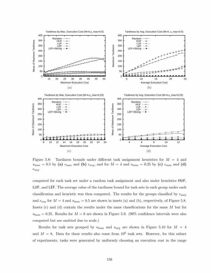
0

50

100

150

200

250

300

350

400

15 20 25 30 35 40 45 50

Mea

n of

Max

imum

Tar

dine

ss

Maximum Execution Cost

Tardiness by Max. Execution Cost (M=4,u_max=0.5)

RandomHUFLUFLEF

LEF+Slicing

(a)

0

50

100

150

200

250

300

350

400

5 10 15 20 25

Max

imum

Tar

dine

ss


Tardiness by Avg. Execution Cost (M=4, u_max=0.5)

RandomHUFLUFLEF

LEF+Slicing

(b)

0

50

100

150

200

250

300

350

400

8 10 12 14 16 18 20 22 24 26

Mea

n of

Max

imum

Tar

dine

ss


Tardiness by Max. Execution Cost (M=4,u_max=0.25)

RandomHUFLUFLEF

LEF+Slicing

(c)

0

50

100

150

200

250

300

350

400

4 6 8 10 12

Mea

n of

Max

imum

Tar

dine

ss


Tardiness by Avg. Execution Cost (M=4,u_max=0.25)

RandomHUFLUFLEF

LEF+Slicing

(d)

Figure 5.8: Tardiness bounds under different task assignment heuristics for M = 4 andumax = 0.5 by (a) emax and (b) eavg, and for M = 4 and umax = 0.25 by (c) emax and (d)eavg.

computed for each task set under a random task assignment and also under heuristics HUF,

LUF, and LEF. The average value of the tardiness bound for task sets in each group under each

classification and heuristic was then computed. The results for the groups classified by emax

and eavg for M = 4 and umax = 0.5 are shown in insets (a) and (b), respectively, of Figure 5.8.

Insets (c) and (d) contain the results under the same classifications for the same M but for

umax = 0.25. Results for M = 8 are shown in Figure 5.9. (99% confidence intervals were also

computed but are omitted due to scale.)

Results for task sets grouped by umax and uavg are shown in Figure 5.10 for M = 4

and M = 8. Data for these results also come from 106 task sets. However, for this subset

of experiments, tasks were generated by uniformly choosing an execution cost in the range

156

0

50

100

150

200

250

300

350

400

20 25 30 35 40 45 50

Mea

n of

Max

imum

Tar

dine

ss


Tardiness by Max. Execution Cost (M=8, u_max=0.5)

RandomHUFLUFLEF

LEF+Slicing

(a)

0

50

100

150

200

250

300

350

400

6 8 10 12 14 16 18 20

Mea

n of

Max

imum

Tar

dine

ss



RandomHUFLUFLEF

LEF+Slicing

(b)

0

50

100

150

200

250

300

350

400

12 14 16 18 20 22 24

Mea

n of

Max

imum

Tar

dine

ss


Tardiness by Max. Execution Cost (M=8, u_max=0.25)

RandomHUFLUFLEF

LEF+Slicing

(c)

0

50

100

150

200

250

300

350

400

4 5 6 7 8 9 10 11

Mea

n of

Max

imum

Tar

dine

ss



RandomHUFLUFLEF

LEF+Slicing

(d)

Figure 5.9: Tardiness bounds under different task assignment heuristics for M = 8 andumax = 0.5 by (a) emax and (b) eavg, and for M = 8 and umax = 0.25 by (c) emax and (d)eavg.

[1.0, 20.0] and a utilization in the range [umin, umax]; the pair (umin, umax) for each task set was

uniformly chosen from those in the set {(0.0, 0.2), (0.0, 0.4), (0.1, 0.5), (0.3, 0.5)}. This strategy

was used so that a sufficient number of task sets fall under each uavg group.

From the plots, we first observe that there is only a slight increase in the tardiness bounds

as the number of processors is increased from four to eight. This is because the tardiness

bound given by (5.21) is independent of M . However, the maximum of the tardiness bounds

computed for all the tasks can be expected to increase as the number of processors, and hence,

the number of tasks increase. The increase, however, seems to be negligible.

Coming to the comparison of the different heuristics, the plots show that LEF guarantees

the minimum tardiness of the four task-assignment approaches. LUF is the next best with the

157

0

50

100

150

200

250

300

350

400

0.2 0.25 0.3 0.35 0.4 0.45 0.5

Mea

n of

Max

imum

Tar

dine

ss

Maximum Utilization

Tardiness by Max. Utilization on 4 processors

RandomHUFLUFLEF

LEF+Slicing

(a)

0

50

100

150

200

250

300

350

400

0.1 0.15 0.2 0.25 0.3 0.35 0.4 0.45

Max

imum

Tar

dine

ss

Average Utilization

Tardiness by Avg. Utilization on 4 processors

RandomHUFLUFLEF

LEF+Slicing

(b)

0

50

100

150

200

250

300

350

400

0.2 0.25 0.3 0.35 0.4 0.45 0.5

Mea

n of

Max

imum

Tar

dine

ss

Maximum Utilization

Tardiness by Max. Utilization on 8 processors

RandomHUFLUFLEF

LEF+Slicing

(c)

0

50

100

150

200

250

300

350

400

0.1 0.15 0.2 0.25 0.3 0.35 0.4 0.45

Max

imum

Tar

dine

ss

Average Utilization

Tardiness by Avg. Utilization on 8 processors

RandomHUFLUFLEF

LEF+Slicing

(d)

Figure 5.10: Tardiness bounds under different task assignment heuristics for (a) M = 4 andumax (b) M = 4 and uavg (c) M = 8 and umax (d) M = 8 and uavg. In all the graphs,emax = 20 and eavg = 10.

difference between LEF and LUF being wider on M = 8 processors than on M = 4 processors.

Another interesting observation is that HUF performs worse than even Random most of the

time. Under LEF, tardiness is quite low (approximately 8 time units mostly) for umax =

0.25 (insets (c) and (d) of Figures 5.8 and 5.9 and insets (a) and (c) of Figure 5.10), which

suggests that LEF may be a reasonable strategy for such task systems. Tardiness increases

with increasing umax, but is still a reasonable value of 25 time units only for eavg ≤ 10 when

umax = 0.5. However, for eavg = 20, tardiness exceeds 75 time units when M = 8, which

may not be acceptable. For such systems, tardiness can be reduced by using the job-slicing

approach, at the cost of increased migration overhead. Therefore, in an attempt to determine

the reduction possible with the job-slicing approach, we also computed the tardiness bound

158

0

20

40

60

80

100

2 4 6 8 10 12 14 16 18

% o

f tas

k se

ts a

ssig

ned

No. of processors (M)

Performance of LUF with non-light tasks

u_max=0.6u_max=0.7u_max=0.8u_max=0.9u_max=1.0

(a)

0

50

100

150

200

250

300

350

400

8 10 12 14 16 18 20 22

Mea

n of

Max

imum

Tar

dine

ss


Estimated and Observed Tardiness under LEF (M=8)

EstimatedObserved

(b)

0

50

100

150

200

250

300

350

400

0.2 0.25 0.3 0.35 0.4

Mea

n of

Max

imum

Tar

dine

ss

Average Utilization

Estimated and Observed Tardiness under LEF (M=8)

EstimatedObserved

(c)

Figure 5.11: (a)Percentage of randomly-generated task sets with heavy tasks successfullyassigned by the LUF heuristic. (b) & (c) Comparison of estimated and observed tardinessunder EDF-fm-LEF by (b) average execution cost and (c) average utilization.

under LEF assuming that each job of a migrating task is sliced into sub-jobs with execution

costs in the range [1, 2). This bound is also plotted in the figures referred to above. For

umax = 0.5, we found the bound to settle to approximately 7–8 time units, regardless of the

execution costs and individual task utilizations. (When umax = 0.25, tardiness is only 1–2 time

units under LEF with job slicing.) In our experiments, on average, a seven-fold decrease in

tardiness was observed with job slicing with a granularity of one to two time units per sub-job.

However, a commensurate increase in the number of migrations is also inevitable.

Overall, the results indicate that the tardiness bounds guaranteed may be tolerable if task

execution costs are not high and the LEF strategy is used for task assignment.

The second set of experiments evaluates the different heuristics in their ability to success-

159

fully assign task sets that contain heavy tasks also. Task sets were generated using the same

procedure as that described for the first set of experiments above, except that umax was varied

between 0.6 and 1.0 in steps of 0.1. All of the four approaches could assign 100% of the task

sets generated for M = 2, as expected. For higher values of M , the success ratio plummeted

for all but the LUF approach. The percentage of task sets that LUF could successfully assign

for varying M and umax is shown in Figure 5.11(a). LEF performed next best (graphs not

provided). However, even when umax = 0.6, its success percentage is approximately 79% when

M = 4 and 24% when M = 16; the corresponding values are approximately 23.9% and 0.3%,

respectively, when umax is increased to 1.0. In this set of experiments also, HUF almost al-

ways performed worse than Random, and its success percentage was close to zero except when

M = 4.

The third set of experiments was designed to evaluate the pessimism in the tardiness bound

of (5.21). 300,000 task sets were generated with umax = 0.5 and Usum = 8. The tardiness

bound estimated by (5.21) under the LEF task assignment heuristic was computed for each

task set. A schedule under EDF-fm-LEF for 100,000 time units was also generated for each task

set (when each task releases jobs in a synchronous, periodic manner) and the actual maximum

tardiness observed was noted. (The time limit of 100,000 was determined by trial-and-error as

an upper bound on the time within which tardiness converged for the tasks sets generated.)

Plots of the average of the estimated and observed values for tasks grouped by eavg and uavg

are shown in insets (b) and (c) of Figure 5.11, respectively. In general, we found that actual

tardiness is only approximately half of the estimated value.

Finally, experiments were run to compare the bounds computed iteratively, which could

require exponential time, to the actual tardiness. For this set of experiments, to facilitate

computations, both periods and execution costs were chosen to be integers. Further, to rea-

sonably constrain the length of the busy interval, the maximum period was restricted to 20,

and some odd values such as 13, 17, and 19 were forbidden. Results are shown in Figure 5.12

and indicate that the bounds computed using this approach are very close to actual tardiness

observed.

5.4 Summary

We have proposed an algorithm, EDF-fm, which is based upon EDF, for scheduling recurrent

soft real-time task systems on multiprocessors, and have derived a tardiness bound that can be

160

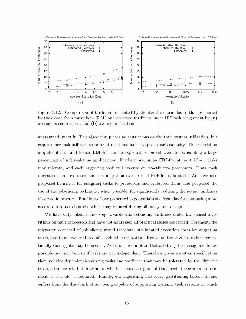
0

5

10

15

20

25

30

35

40

2 2.5 3 3.5 4 4.5 5 5.5 6

Mea

n of

Max

imum

Tar

dine

ss


Estimated (Non-Iterative and Iterative) and Observed Tardiness under LEF (M=4)

Estimated (Non-Iterative)Estimated (Iterative)

Observed

(a)

0

5

10

15

20

25

30

35

40

0.2 0.25 0.3 0.35 0.4 0.45

Mea

n of

Max

imum

Tar

dine

ss

Average Utilization

Estimated (Non-Iterative and Iterative) and Observed Tardiness under LEF (M=4)

Estimated (Non-Iterative)Estimated (Iterative)

Observed

(b)

Figure 5.12: Comparison of tardiness estimated by the iterative formulas to that estimatedby the closed-form formula in (5.21) and observed tardiness under LEF task assignment by (a)average execution cost and (b) average utilization.

guaranteed under it. This algorithm places no restrictions on the total system utilization, but

requires per-task utilizations to be at most one-half of a processor’s capacity. This restriction

is quite liberal, and hence, EDF-fm can be expected to be sufficient for scheduling a large

percentage of soft real-time applications. Furthermore, under EDF-fm, at most M − 1 tasks

may migrate, and each migrating task will execute on exactly two processors. Thus, task

migrations are restricted and the migration overhead of EDF-fm is limited. We have also

proposed heuristics for assigning tasks to processors and evaluated them, and proposed the

use of the job-slicing technique, when possible, for significantly reducing the actual tardiness

observed in practice. Finally, we have presented exponential-time formulas for computing more

accurate tardiness bounds, which may be used during offline system design.

We have only taken a first step towards understanding tardiness under EDF-based algo-

rithms on multiprocessors and have not addressed all practical issues concerned. Foremost, the

migration overhead of job slicing would translate into inflated execution costs for migrating

tasks, and to an eventual loss of schedulable utilization. Hence, an iterative procedure for op-

timally slicing jobs may be needed. Next, our assumption that arbitrary task assignments are

possible may not be true if tasks are not independent. Therefore, given a system specification

that includes dependencies among tasks and tardiness that may be tolerated by the different

tasks, a framework that determines whether a task assignment that meets the system require-

ments is feasible, is required. Finally, our algorithm, like every partitioning-based scheme,

suffers from the drawback of not being capable of supporting dynamic task systems in which

161

the set of tasks and task parameters can change at run-time. We defer addressing these issues

to future work.

162

Chapter 6

A Schedulable Utilization Bound for EPDF1

In this chapter, we derive a schedulable utilization bound for the earliest-pseudo-deadline-

first (EPDF) Pfair scheduling algorithm on multiprocessors. EPDF is not optimal but is less

expensive than some other known Pfair algorithms. A motivation for determining a schedulable

utilization bound for EPDF is provided in Section 6.1 below, which is followed by a derivation

in Section 6.2. Proofs omitted from this chapter are provided in Appendix C.

6.1 Introduction and Motivation

In the previous two chapters, we considered scheduling soft real-time systems under preemptive

and non-preemptive global EDF (g-EDF and g-NP-EDF), and EDF-fm, a restricted-migration

algorithm based on partitioned EDF. Although g-EDF and g-NP-EDF can guarantee bounded

tardiness to every task system that is feasible on M processors, their tardiness bounds can

exceed the tolerance limits of some applications. EDF-fm also suffers from this drawback,

apart from two others. First, EDF-fm cannot guarantee bounded tardiness to all feasible task

systems with umax > 0.5. Second, its partitioning-based design, which makes it attractive to

static task systems and task systems with large migration overheads, renders it unsuitable for

dynamic task systems.

Pfair scheduling algorithms, which schedule tasks one quantum at a time, do not suffer

from the above drawbacks. Though tasks may be prone to frequent migrations due to their

1Contents of this chapter previously appeared in preliminary form in the following paper:[49] U. Devi and J. Anderson. Schedulable utilization bounds for EPDF fair multiprocessor scheduling. InProceedings of the 10th International Conference on Real-Time and Embedded Computing Systems and Appli-

cations, Springer-Verlag Lecture Notes in Computer Science, pages 261–280, August 2004.

quantum-based scheduling, as explained in Chapter 1, Pfair algorithms are still of interest in

systems in which the gain in schedulability or the decrease in tardiness outweighs the loss in

utilization due to migration overheads.

As discussed in Chapter 1, some restrictions and/or requirements of optimal Pfair algo-

rithms can be overkill for soft real-time systems. If small tardiness bounds can be guaranteed

under simpler algorithms in which one or more of those requirements are eliminated, then

such algorithms may be sufficient for soft real-time systems. In this and the next chapter, we

consider the earliest-pseudo-deadline-first (EPDF) algorithm, which is one such simpler, but

non-optimal, Pfair algorithm.

EPDF is more efficient than optimal Pfair algorithms in that it does not use any tie-

breaking rule to resolve ties among subtasks with the same pseudo-deadline, but disambiguates

ties arbitrarily. PD2, the most efficient of the known optimal Pfair algorithms, requires two

tie-break parameters, the b-bit and group deadline, which were described in Chapter 3 in

detail. Though these tie-break parameters can be computed for each subtask in constant time,

there exist some soft and/or dynamic real-time systems in which not using them may still be

preferable. Eliminating tie-breaking rules may also be preferable in embedded systems with

slower processors or limited memory bandwidth.

The viability of EPDF for scheduling soft and/or dynamic real-time systems was first con-

sidered by Srinivasan and Anderson in [106], where they provide examples of such applications

for which EPDF may be preferable to PD2. Some web-hosting systems, server farms, packet

processing in programmable multiprocessor-based routers, and packet transmission on multi-

ple, parallel outgoing router links are among examples provided by them. In these systems, fair

resource allocation is needed, so that quality-of-service guarantees can be provided. However,

an extreme notion of fairness that precludes all deadline misses is not required. Moreover, in

systems such as routers, the inclusion of tie-breaking information in subtask priorities may

result in unacceptably high space overhead.

The applications mentioned above may also be dynamic in that the set of tasks and the

utilizations of tasks requiring service may be in a constant flux. In [106], Srinivasan and An-

derson also noted that the use of tie-breaking rules may be problematic for such dynamic task

systems. As they explain, it is possible to reweight each task whenever its utilization changes

such that its next subtask deadline is preserved. If no tie-breaking information is maintained,

such an approach entails very little computational overhead. However, utilization changes can

cause tie-breaking information to change, so if tie-breaking rules are used, reweighting may

164

necessitate an O(N) cost for N tasks, due to the need to re-sort the scheduler’s priority queue.

This cost may be prohibitive if reallocations are frequent.

Motivated by the above reasons, Srinivasan and Anderson studied EPDF and they suc-

ceeded in showing that EPDF can guarantee a tardiness bound of one quantum for every

subtask, provided a certain condition holds. Their condition can be ensured by limiting each

task’s weight to at most 1/2, and can be generalized to apply to tardiness bounds higher than

one. Unfortunately, Srinivasan and Anderson left open the question of whether such conditions

are necessary to guarantee small constant tardiness.

We address the issues left open by Srinivasan and Anderson with respect to EPDF for

soft real-time systems in the next chapter. Before doing so, in this chapter, we consider the

following question, which is orthogonal to that addressed in prior work: If individual tasks

cannot be subject to weight restrictions, then what would be a sufficient restriction on the

total utilization of a task system for it to be scheduled correctly under EPDF? We answer this

question by deriving a schedulable utilization bound for EPDF. The concept of schedulable

utilization bound and its use were described in Chapter 1 in Section 1.4. Answering this

question should help in identifying the conditions for which the soft real-time scheduling results

of EPDF are applicable. Also, if the total utilization of an EPDF-scheduled soft real-time system

is less than the schedulable utilization bound of EPDF, then that system can be treated as a

hard real-time system.

In this chapter, we show that on M processors, EPDF can correctly schedule every

task system τ with total utilization at most min(M, λM(λ(1+Wmax)−Wmax)+1+Wmax

λ2(1+Wmax)), where

Wmax = umax(τ) and λ = max(2,⌈

1Wmax

⌉

). For Wmax ≥ 12 , i.e., λ = 2, this value reduces

to (2M+1)(2+Wmax)−14(1+Wmax) , and as Wmax → 1.0, it approaches 3M+1

4 , which, as M → ∞, approaches

3M4 , i.e., 75% of the total processing capacity. When Wmax > 1/2, the utilization bound that

we have derived for EPDF is greater than that of every known non-Pfair algorithm by around

25%. Currently, it is not known whether 3M+14 is a worst-case, let alone, optimal utilization

bound for EPDF. The closest that we have come in assessing the accuracy of our result is a

counterexample that shows that when Wmax ≥ 56 , worst-case schedulable utilization cannot

exceed 86%. We have also considered extending this result for use in systems where tardiness

may be permissible. This extension is presented along with the associated analysis in the next

chapter.

165

6.2 A Schedulable Utilization Bound for EPDF

In this section, we derive a schedulable utilization bound for EPDF. The utilization bound that

we derive is more accurate than that specified in Section 6.1, and can be used if the ρ values

of tasks as defined in (6.1) can be computed.

Before getting started, we will define needed notation. Let ρ, ρmax, Wmax, and λ be defined

as follows. (The task system τ will be omitted when it is unambiguous.)

ρ(T )def= (T.e − gcd(T.e, T.p))/T.p (6.1)

ρmax(τ)def= max

T∈τ{ρ(T )} (6.2)

Wmax(τ)def= max

T∈τ{wt(T )} (6.3)

λ(τ)def= max

(

2,

⌈

1

Wmax(τ)

⌉)

(6.4)

The utilization bound that we derive for EPDF is given by the following theorem.

Theorem 6.1 Every GIS task system τ with total system utilization,∑

T∈τ wt(T ), at most

min(

M, λM(λ(1+ρmax)−ρmax)+1+ρmax

λ2(1+ρmax)

)

, where ρmax and λ are as defined in (6.2) and (6.4), re-

spectively, is correctly scheduled by EPDF on M processors.

As a shorthand, we define U(M,k, f) as follows.

Definition 6.1: U(M,k, f)def= kM(k(1+f)−f)+1+f

k2(1+f).

We use a setup similar to that used by Srinivasan and Anderson in [105] in establishing

the optimality of PD2 to prove the above theorem. The overall strategy is to assume that the

theorem is false, identify a task system that is minimal or smallest in the sense of having the

smallest number of subtasks and that misses its deadline, and show that such a task system

cannot exist. (It should be pointed out that although the setup is similar, the details of the

derivation and proof are significantly different.)

If Theorem 6.1 does not hold, then there exist a Wmax ≤ 1 and ρmax < 1, and a time td

and a concrete task system τ defined as follows. (In these definitions, we assume that τ is

scheduled on M processors.)

Definition 6.2: td is the earliest time at which any concrete task system with each task

weight at most Wmax, ρ(T ) at most ρmax for each task T , and total utilization at most

166

min(M,U(M,λ, ρmax)) misses a deadline under EPDF, i.e., some such task system misses

a subtask deadline at td, and no such system misses a subtask deadline prior to td.

Definition 6.3: τ is a task system with the following properties.

(T0) τ is concrete task system with each task weight at most Wmax, ρ(T ) at most ρmax, and

total utilization at most min(M,U(M,λ, ρmax)).

(T1) A subtask in τ misses its deadline at td in S, an EPDF schedule for τ .

(T2) No concrete task system satisfying (T0) and (T1) releases fewer subtasks in [0, td) than

τ .

(T3) No concrete task system satisfying, (T0), (T1), and (T2) has a larger rank than τ at td,

where the rank of a task system τ at t is the sum of the eligibility times of all subtasks with

deadlines at most t, i.e., rank(τ, t) =∑

{Ti:T∈τ ∧ d(Ti)≤t} e(Ti).

(T2) can be thought of as identifying a minimal task system in the sense of having a dead-

line miss with the fewest number of subtasks, subject to satisfying (T0) and (T1). It is easy

to see that if Theorem 6.1 does not hold for all task systems satisfying (T0) and (T1), then

some task system satisfying (T2) necessarily exists. (T3) further restricts the nature of τ by

requiring subtask eligibility times to be spaced as much apart as possible.

The following shorthand notation will be used hereafter.

Definition 6.4: α denotes the total utilization of τ , expressed as a fraction of M , i.e.,

αdef=

∑

T∈τ wt(T )

M .

Definition 6.5: δdef= ρmax

1+ρmax.

The lemma below follows from (T0) and the definition of α.

Lemma 6.1 0 ≤ α ≤ min(M,U(M,λ,ρmax))M ≤ 1.

The next lemma is immediate from the definition of δ, (6.2), and (6.1). A proof is provided in

Appendix C.

Lemma 6.2 0 ≤ δ < 12 .

We now prove some properties about τ and S. In proving some of these properties, we

make use of the following three lemmas established in prior work by Srinivasan and Anderson.

167

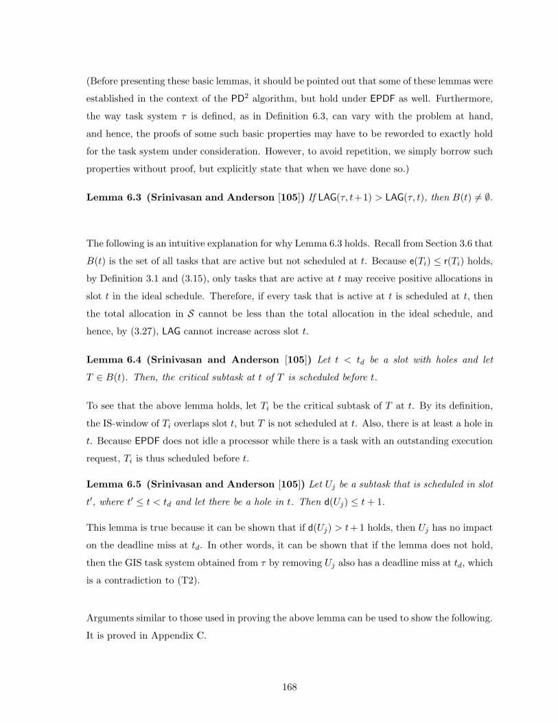
(Before presenting these basic lemmas, it should be pointed out that some of these lemmas were

established in the context of the PD2 algorithm, but hold under EPDF as well. Furthermore,

the way task system τ is defined, as in Definition 6.3, can vary with the problem at hand,

and hence, the proofs of some such basic properties may have to be reworded to exactly hold

for the task system under consideration. However, to avoid repetition, we simply borrow such

properties without proof, but explicitly state that when we have done so.)

Lemma 6.3 (Srinivasan and Anderson [105]) If LAG(τ, t+1) > LAG(τ, t), then B(t) 6= ∅.

The following is an intuitive explanation for why Lemma 6.3 holds. Recall from Section 3.6 that

B(t) is the set of all tasks that are active but not scheduled at t. Because e(Ti) ≤ r(Ti) holds,

by Definition 3.1 and (3.15), only tasks that are active at t may receive positive allocations in

slot t in the ideal schedule. Therefore, if every task that is active at t is scheduled at t, then

the total allocation in S cannot be less than the total allocation in the ideal schedule, and

hence, by (3.27), LAG cannot increase across slot t.

Lemma 6.4 (Srinivasan and Anderson [105]) Let t < td be a slot with holes and let

T ∈ B(t). Then, the critical subtask at t of T is scheduled before t.

To see that the above lemma holds, let Ti be the critical subtask of T at t. By its definition,

the IS-window of Ti overlaps slot t, but T is not scheduled at t. Also, there is at least a hole in

t. Because EPDF does not idle a processor while there is a task with an outstanding execution

request, Ti is thus scheduled before t.

Lemma 6.5 (Srinivasan and Anderson [105]) Let Uj be a subtask that is scheduled in slot

t′, where t′ ≤ t < td and let there be a hole in t. Then d(Uj) ≤ t + 1.

This lemma is true because it can be shown that if d(Uj) > t+1 holds, then Uj has no impact

on the deadline miss at td. In other words, it can be shown that if the lemma does not hold,

then the GIS task system obtained from τ by removing Uj also has a deadline miss at td, which

is a contradiction to (T2).

Arguments similar to those used in proving the above lemma can be used to show the following.

It is proved in Appendix C.

168

Lemma 6.6 Let t < td be a slot with holes and let Uj be a subtask that is scheduled at t. Then

d(Uj) = t + 1 and b(Uj) = 1.

Finally, we will also use the following lemma, which is a generalization of Lemma 6.3. It is

also proved in Appendix C.

Lemma 6.7 If LAG(τ, t+1) > LAG(τ, t−`), where 0 ≤ ` ≤ λ−2 and t ≥ `, then B(t−`, t+1) 6=∅.

The next lemma establishes some properties concerning S.

Lemma 6.8 The following properties hold for τ and S.

(a) For all Ti in τ , d(Ti) ≤ td.

(b) Exactly one subtask of τ misses its deadline at td.

(c) LAG(τ, td) = 1.

(d) Let Ti be a subtask in τ that is scheduled at t < td in S. Then, e(Ti) = min(r(Ti), t).

(e) (∀Ti ∈ τ :: d(Ti) < td ⇒ (∃t :: e(Ti) ≤ t < d(Ti) ∧ S(Ti, t) = 1)). That is, every subtask

with deadline before td is scheduled before its deadline.

(f) Let Uk be the subtask in τ that misses its deadline at td. Then, U is not scheduled in any

slot in [td − λ + 1, td).

(g) There is no hole in any of the last λ − 1 slots, i.e., in slots [td − λ + 1, td).

(h) There exists a time v ≤ td − λ such that the following both hold.

(i) There is no hole in any slot in [v, td − λ).

(ii) LAG(τ, v) ≥ (td − v)(1 − α)M + 1.

(i) There exists a time u ∈ [0, v), where v is as defined in part (h), such that LAG(τ, u) < 1

and LAG(τ, t) ≥ 1 for all t in [u + 1, v].

The proofs of parts (a)–(d) are similar to those formally proved in [105] for the optimal

PD2 Pfair algorithm. We give informal explanations here. Part (e) follows directly from

Definition 6.2 and (T1). The rest are proved in Appendix C.

Proof of (a): This part holds because a subtask with deadline after td cannot impact the

schedule for those with deadlines at most td. Therefore, even if all the subtasks with deadlines

after td are removed, the deadline miss at td cannot be eliminated. This contradicts (T2).

169

Proof of (b): If several subtasks miss their deadlines at td, then even if all but one are

removed, the remaining subtask will still miss its deadline, contradicting (T2).

Proof of (c): By part (a), all the subtasks in τ complete executing in the ideal schedule by

td. Hence, the total allocation to τ in the ideal schedule up to td is exactly equal to the total

number of subtasks in τ . By part (b), the total number of subtasks of τ scheduled in S in the

same interval is fewer by exactly one subtask. Hence, the difference in allocations, LAG(τ, td),

is exactly one quantum.

Proof of (d): Suppose e(Ti) is not equal to min(r(Ti), t). Then, by (3.12) and because Ti

is scheduled at t, it is before min(r(Ti), t). Hence, simply changing e(Ti) so that it equals

min(r(Ti), t) will not affect how Ti or any other subtask is scheduled. So, the deadline miss at

td will persist. However, this change increases the rank of the task system, and hence, (T3) is

contradicted. �

Overview of the rest of the proof of Theorem 6.1. If td and τ as given by Definitions 6.2

and 6.3, respectively, exist, then by Lemma 6.8(i), there exists a time slot u < v, where v is as

defined in Lemma 6.8(h), across which LAG increases to at least one. To prove Theorem 6.1,

we show that for every such u, either (i) there exists a time u′, where u + 1 < u′ ≤ v or

u′ = td, such that LAG(τ, u′) < 1, and thereby derive a contradiction to either Lemma 6.8(i)

or Lemma 6.8(c), or (ii) v referred to above does not exist, contradicting Lemma 6.8(h). The

crux of the argument we use in establishing the above is as follows. By Lemma 3.4, for LAG

to increase across slot u, at least one hole is needed in that slot. We show that for every such

slot, there are a sufficient number of slots without holes, and hence, that if (T0) holds, then

the increase in LAG across slot u is offset by a commensurate decrease in LAG elsewhere that

is sufficient to ensure that no deadline is missed.

In what follows, we state and prove several other lemmas that are required to accomplish

this. We begin with a simple lemma that relates PF-window lengths to λ.

Lemma 6.9 If Wmax < 1, then the length of the PF-window of each subtask of each task T

in τ is at least λ; otherwise, it is at least λ − 1.

Proof: Follows from the definition of λ in (6.4) and Lemma 3.1. �

170

The next lemma involves subtask release times and deadlines and is proved in Appendix C.

Lemma 6.10 For all i ≥ 1, k ≥ 1, the following holds.

r(Ti+k) ≥

d(Ti) + k − 1, b(Ti) = 0

d(Ti) + k − 2, b(Ti) = 1

The lemma that follows shows that LAG does not increase across the first λ − 1 slots, i.e.,

across slots 0, 1, . . . , λ − 2.

Lemma 6.11 (∀t : 0 ≤ t ≤ λ − 2 :: LAG(τ, t + 1) ≤ LAG(τ, t)).

Proof: Contrary to the statement of the lemma, assume that LAG(τ, t + 1) > LAG(τ, t) for

some 0 ≤ t ≤ λ−2. Then, by Lemma 3.4, there is at least one hole in slot t, and by Lemma 6.3,

B(t) is not empty. Let U be a task in B(t) and Uj its critical subtask at t. Because there is a

hole in t, by Lemma 6.4,

(B) Uj is scheduled before t,

and hence, by Lemma 6.5, d(Uj) ≤ t+1 holds. We will consider two cases depending on Wmax.

If Wmax < 1, then by Lemma 6.9, |ω(Uj)| (i.e., the length of the PF-window of Uj) is at least

λ, and hence, by Lemma 3.1, r(Uj) = d(Uj) − |ω(Uj)| ≤ t + 1 − λ holds. By our assumption,

t < λ − 1, and hence, r(Uj) < 0, which is impossible. Thus, the lemma holds when Wmax < 1.

On the other hand, if Wmax = 1, then, by (6.4), λ = 2 holds, and hence, by our assumption,

t = 0. Therefore, by (B), Uj is scheduled before time zero, which is also impossible. The

lemma follows. �

Lemma 3.4 showed that at least one hole is necessary in slot t for LAG to increase across

t. The next lemma relates an increase in LAG to certain other conditions.

Lemma 6.12 The following properties hold for LAG in S.

(a) If LAG(τ, t + 1,S) > LAG(τ, t,S), where λ − 1 ≤ t < td − λ, then there is no hole in any

slot in [t − λ + 2, t).

(b) If LAG(τ, t + 1,S) > LAG(τ, t − λ + 2,S), then there is no hole in slot t − λ + 1.

Proof: We prove the two parts separately.

171

Proof of part (a). By the definition of λ in (6.4), λ ≥ 2 holds. If λ = 2, then this part is

vacuously true. Therefore, assume λ ≥ 3, which, by (6.4), implies that

Wmax <1

2. (6.5)

Because LAG(τ, t + 1) > LAG(τ, t), by Lemma 3.4,

(H) there is at least one hole in slot t,

and by Lemma 6.3, B(t) is not empty. Let U be a task in B(t) and let Uj be the critical

subtask of U at t. By (H) and Lemma 6.4, Uj is scheduled before t. Let Uj be scheduled at

t′ < t, i.e.,

S(Uj , t′) = 1 ∧ t′ < t. (6.6)

Also, by Definition 3.2, d(Uj) ≥ t+1 holds, while by (H), (6.6), and Lemma 6.5, d(Uj) ≤ t+1

holds. Hence, we have

d(Uj) = t + 1. (6.7)

By (6.5) and Lemma 6.9, the length of Uj ’s PF-window, |ω(Uj)| ≥ λ, and hence, by (6.7)

and the definition of PF-window in Lemma 3.1, r(Uj) ≤ t − λ + 1. We claim that Uj can be

scheduled at ar after t − λ + 2. If there does not exist a predecessor for Uj , then Uj can be

scheduled any time at or after r(Uj), and hence, at or after t − λ + 1. If not, let Uh be the

predecessor of Uj. Then, h ≤ j, and hence, by Lemma 6.10, d(Uh) ≤ t − λ + 2 holds. By

Lemma 6.8(e), Uh does not miss its deadline, and hence, is scheduled at or before t − λ + 1.

This implies that Uj is ready and can be scheduled at any time at or after t − λ + 2. Given

this, if t′ > t− λ + 2, then there is no hole in any slot in [t− λ + 2, t′). Hence, to complete the

proof, it is sufficient to show that there is no hole in any slot in [t′, t). Assume to the contrary,

and let v be the earliest slot with at least one hole in [t′, t). Then, by (6.6) and Lemma 6.5,

d(Uj) ≤ v + 1 ≤ t, which contradicts (6.7). Thus, v does not exist, and there is no slot with

one or more holes in [t′, t).

Proof of part (b). By the statement of this part of the lemma, LAG(τ, t + 1) > LAG(τ, t −λ + 2). Hence, Lemma 6.7 applies with ` = λ − 2. Therefore, B(t− λ + 2, t + 1) is not empty.

By definition, a task in B(t − λ + 2, t + 1) is not scheduled anywhere in [t − λ + 2, t + 1). Let

U be a task in B(t − λ + 2, t + 1) and let t − λ + 2 ≤ v ≤ t be the latest slot in the interval

[t − λ + 2, t + 1) in which U is active, and let Uj be its critical subtask at v. Therefore, by

172

Definition 3.2,

d(Uj) ≥ v + 1 ≥ t − λ + 3. (6.8)

By Lemma 3.4, there is at least one hole in the interval [t − λ + 2, t + 1). Hence, because U

is in B(t − λ + 2, t + 1), and thus is not scheduled anywhere in the interval concerned, Uj is

scheduled at or before t− λ + 1 (as opposed to after the interval under consideration). Hence,

if there is a hole in t − λ + 1, then by Lemma 6.5, it follows that d(Uj) ≤ t − λ + 1, which

contradicts (6.8). Hence, there cannot be any hole in t − λ + 1, which completes the proof of

this part. �

The next lemma bounds the lag of each task at time t + 1, where t is a slot with one or

more holes.

Lemma 6.13 If t < td is a slot with one or more holes in S. Then the following hold.

(a) (∀T ∈ A(t) :: 0 ≤ lag(T, t + 1) ≤ ρ(T ))

(b) (∀T ∈ B(t) :: lag(T, t + 1) = 0)

(c) (∀T ∈ I(t) :: lag(T, t + 1) = 0)

Proof: Part (c) has been proved formally in [106]. To see why part (c) holds, note that no

task in I(t) is scheduled at t. Because there is a hole in t, the latest subtask of a task in I(t)

with release time at or before t should have completed execution by t. Hence, such a task

cannot be behind with respect to the ideal schedule.

Proof of part (a). Let T be a task in A(t) and let Ti be its subtask scheduled at t. Then, in

S, Ti and all prior subtasks of T are scheduled in [0, t+1), i.e., each of these subtasks receives

its entire allocation of one quantum in [0, t + 1). Because there is a hole in t, by Lemma 6.6,

we have

d(Ti) = t + 1 ∧ b(Ti) = 1. (6.9)

By (3.17) and the final part of (3.15), this implies that Ti and all prior subtasks of T receive

a total allocation of one quantum each in [0, t + 1) in the ideal schedule also. Therefore, any

difference in the allocations received in the ideal schedule and S is only due to subtasks that

are released later than Ti. This is illustrated in Figure 6.1. Further, this difference can only be

positive, and hence, the lower bound holds. We next show that the upper bound also holds.

Obviously, in S, every subtask that is released later than Ti receives an allocation of zero

in [0, t+1). Therefore, the lag of T at t+1 is equal to the allocations that these later subtasks

receive in the ideal schedule in the same interval. To determine this value, let Tj be the

173

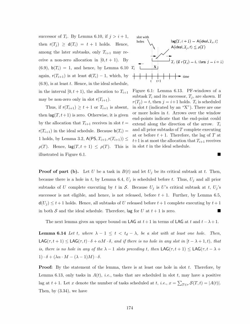
X

timet t+1

slot withholes

] _ a b_] cdef ghijk dlmnc]o

p_qrstuv] vec wx_]cuty_]vemncdp_qrstuv] vec

Figure 6.1: Lemma 6.13. PF-windows of asubtask Ti and its successor, Tj , are shown. Ifr(Tj) = t, then j = i+1 holds. Ti is scheduledin slot t (indicated by an “X”). There are oneor more holes in t. Arrows over the windowend-points indicate that the end-point couldextend along the direction of the arrow. Ti

and all prior subtasks of T complete executingat or before t + 1. Therefore, the lag of T att+1 is at most the allocation that Ti+1 receivesin slot t in the ideal schedule.

successor of Ti. By Lemma 6.10, if j > i + 1,

then r(Tj) ≥ d(Ti) = t + 1 holds. Hence,

among the later subtasks, only Ti+1 may re-

ceive a non-zero allocation in [0, t + 1). By

(6.9), b(Ti) = 1, and hence, by Lemma 6.10

again, r(Ti+1) is at least d(Ti) − 1, which, by

(6.9), is at least t. Hence, in the ideal schedule,

in the interval [0, t + 1), the allocation to Ti+1

may be non-zero only in slot r(Ti+1).

Thus, if r(Ti+1) ≥ t + 1 or Ti+1 is absent,

then lag(T, t+1) is zero. Otherwise, it is given

by the allocation that Ti+1 receives in slot t =

r(Ti+1) in the ideal schedule. Because b(Ti) =

1 holds, by Lemma 3.2, A(PS, Ti+1, r(Ti+1)) ≤ρ(T ). Hence, lag(T, t + 1) ≤ ρ(T ). This is

illustrated in Figure 6.1. �

Proof of part (b). Let U be a task in B(t) and let Uj be its critical subtask at t. Then,

because there is a hole in t, by Lemma 6.4, Uj is scheduled before t. Thus, Uj and all prior

subtasks of U complete executing by t in S. Because Uj is U ’s critical subtask at t, Uj ’s

successor is not eligible, and hence, is not released, before t + 1. Further, by Lemma 6.5,

d(Uj) ≤ t + 1 holds. Hence, all subtasks of U released before t + 1 complete executing by t + 1

in both S and the ideal schedule. Therefore, lag for U at t + 1 is zero. �

The next lemma gives an upper bound on LAG at t+1 in terms of LAG at t and t−λ+1.

Lemma 6.14 Let t, where λ − 1 ≤ t < td − λ, be a slot with at least one hole. Then,

LAG(τ, t + 1) ≤ LAG(τ, t) · δ + αM · δ, and if there is no hole in any slot in [t − λ + 1, t), that

is, there is no hole in any of the λ − 1 slots preceding t, then LAG(τ, t + 1) ≤ LAG(τ, t − λ +

1) · δ + (λα · M − (λ − 1)M) · δ.

Proof: By the statement of the lemma, there is at least one hole in slot t. Therefore, by

Lemma 6.13, only tasks in A(t), i.e., tasks that are scheduled in slot t, may have a positive

lag at t + 1. Let x denote the number of tasks scheduled at t, i.e., x =∑

T∈τ S(T, t) = |A(t)|.Then, by (3.34), we have

174

LAG(τ, t + 1) ≤ ∑

T∈A(t) lag(T, t + 1)

≤ ∑

T∈A(t) ρ(T ) (by Lemma 6.13)

≤ ∑

T∈A(t) ρmax (by (6.2))

= |A(t)| · ρmax

= x · ρmax. (6.10)

Using (3.29), LAG(τ, t + 1) can be expressed as follows.

LAG(τ, t + 1) ≤ LAG(τ, t) +∑

T∈τ (wt(T ) − S(T, t))

= LAG(τ, t) +∑

T∈τ wt(T ) − x (∑

T∈τ S(T, t) = x)

= LAG(τ, t) + αM − x (by Def. 6.4) (6.11)

By (6.10) and (6.11), we have

LAG(τ, t + 1) ≤ min(x · ρmax,LAG(τ, t) + αM − x).

Because ρmax ≥ 0, and hence, x ·ρmax is non-decreasing with increasing x, whereas LAG(τ, t)+

αM − x is decreasing, LAG(τ, t + 1) is maximized when x · ρmax = LAG(τ, t) + αM − x, i.e.,

when x = LAG(τ, t) · 11+ρmax

+ αM 11+ρmax

. Therefore, using either (6.10) or (6.11), we have

LAG(τ, t + 1) ≤ LAG(τ, t) ·(

ρmax

1+ρmax

)

+ αM ·(

ρmax

1+ρmax

)

= LAG(τ, t) · δ + αM · δ (by Def. 6.5). (6.12)

By the statement of the lemma, t ≥ λ − 1, and hence, t − λ + 1 ≥ 0 holds. Therefore, using

(3.31), LAG(τ, t) can be expressed as follows.

LAG(τ, t) ≤ LAG(τ, t − λ + 1) + (λ − 1) ·∑T∈τ wt(T ) −∑u=t−1u=t−λ+1

∑

T∈τ S(T, u)

If there is no hole in any slot in [t−λ+1, t), then∑

T∈τ S(T, u) = M , for all u in [t−λ+1, t).

Hence,

LAG(τ, t) ≤ LAG(τ, t − λ + 1) + (λ − 1) ·∑T∈τ wt(T ) −∑u=t−1u=t−λ+1

∑

T∈τ S(T, u)

= LAG(τ, t − λ + 1) + (λ − 1) ·∑T∈τ wt(T ) − (λ − 1) · M≤ LAG(τ, t − λ + 1) + (λ − 1)α · M − (λ − 1)M (by Def. 6.4). (6.13)

Substituting (6.13) in (6.12), we have LAG(τ, t+1) ≤ LAG(τ, t−λ+1)·δ+(λα ·M−(λ−1)M)·δ.�

175

The next two lemmas are purely mathematical and are proved in Appendix C. They will

be used in proving a later lemma.

Lemma 6.15 A solution to the recurrence

L0 < δ + δ · αM

Lk ≤ δ · Lk−1 + δ · (λαM − (λ − 1)M),

for all k ≥ 1 and 0 ≤ δ < 1, is given by

Ln < δn+1(1 + αM) + (1 − δn)

(

δ

1 − δ

)

(λαM − (λ − 1)M), for all n ≥ 0.

Lemma 6.16 M(λ−δ−(λ−1)δn+1)+δn+2−δn+1+1−δM(λ−(λ−1)δn+1−δn+2)

≥ M(λ−δ)+ 1λ

λM holds for all n ≥ 0, 0 ≤ δ ≤ 1/2,

and M ≥ 1.

We will next show how to bound LAG at the end of an interval that does not contain λ

consecutive slots without holes, after LAG increases to one at the beginning of the interval.

Lemma 6.17 Let t, where λ− 1 ≤ t < td −λ, be a slot across which LAG increases to at least

one, i.e.,

λ − 1 ≤ t < td − λ ∧ LAG(τ, t) < 1 ∧ LAG(τ, t + 1) ≥ 1. (6.14)

Let u, where t < u ≤ td − λ, be such that there is at least one hole in at least one slot in every

λ consecutive slots in the interval [t + 1, u). Then, LAG(τ, u) < (λ − λα)M + 1.

Proof: Because LAG(τ, t + 1) > LAG(τ, t) holds by (6.14), by Lemmas 3.4 and 6.12, we have

(C1) and (C2) below, respectively. ((C2) holds by part (a) of Lemma 6.12 when λ > 2 and by

part (b) of the same Lemma when λ = 2. By (6.4), λ ≥ 2 holds.)

(C1) There is at least one hole in slot t.

(C2) There is no hole in slot t − 1.

By the statement of the lemma (that there is at least one hole in at least one slot in every

λ consecutive slots in [t+1, u)) and (C1), there is at least one hole in at least one slot in every

λ consecutive slots in [t, u). Therefore, at most λ − 1 consecutive slots in the interval can be

without any hole. Let

n ≥ 0 (6.15)

176

......

......... ...

≤ u − λ

o

holes

holes

holes

Noholes

holes

holes

No

holes

holes

No

holes

Noholes

holes

No

holes

At least onehole in atleast one slotin any λ − 1consecutiveslots



I1

I2, . . . , In−1

In

λ − 1

t tns

I0

t − 1

λ − 1

t + 1 t1h= tn

t1ft0f= t0s = t0h

= t1

= t1s = t2s

= t2

holes or

no holes

holes or

no holes

tnf = utnh u − λ + 1

N

Figure 6.2: Lemma 6.17. LAG(τ, t) < 1 and LAG(τ, t + 1) ≥ 1. There is at least one hole in atleast one slot in every λ consecutive slots in [t − 1, u). Each interval Ik, where 1 ≤ k ≤ n − 1,has one block of λ − 1 consecutive slots without holes; In may have a second block beginningat u − λ + 1. The objective is to determine an upper bound on LAG(τ, u).

denote the number of slots in [t, u − λ + 1) that each begin a block of λ − 1 consecutive slots

with no holes. Note that the last slot in the last block is before u−1. If n > 0, let t1, t2, . . . , tn,

where t1 < t2 < . . . < tn < u − λ + 1 be such slots. Also note that if there is no hole in

[u − λ + 1, u) (provided u − λ + 1 > t + 1 holds), then there is at least one hole in u − λ. By

(C1), t1 > t holds. Further, tn + λ − 1 < u and there is no hole in [ti, ti + λ − 1) for each i.

Because there is at least one hole in at least one slot in any consecutive λ slots in [t, u), there

is at least one hole in ti − 1 for all 1 ≤ i ≤ n. Similarly, there is at least one hole in ti + λ − 1

for all 1 ≤ i ≤ n. Also,

ti+1 − ti ≥ λ, for all 1 ≤ i ≤ n − 1. (6.16)

We divide the interval [t − 1, u) into n + 1 non-overlapping subintervals that each start at

t or at one of the n slots that begin blocks of λ − 1 consecutive slots without holes, namely,

t1, . . . , tn, as shown in Figure 6.2. Note that t − 1 exists by the statement of the lemma, and

by (C2), there is no hole in slot t − 1. Also, as noted earlier, t1 > t.

The subintervals denoted I0, I1, . . . , In are defined as follows.

I0def=

[t − 1, t1), if t1 exists, i.e., n > 0

[t − 1, u), otherwise(6.17)

Indef= [tn, u), if n > 0 (6.18)

Ikdef= [tk, tk+1), for all 1 ≤ k < n (6.19)

177

Before proceeding further, we introduce some more notation. We denote the start and end

times of Ik, where 0 ≤ k ≤ n, by tks and tkf , respectively, i.e., Ik is denoted as follows.

Ikdef= [tks , t

kf ), for all k = 0, 1, . . . , n (6.20)

tkh is defined as follows for 0 ≤ k ≤ n.

tkhdef=

t + 1, k = 0

tks + λ, otherwise(6.21)

LAG at tkh is denoted Lk, i.e.,

Lkdef= LAG(τ, tkh), for all k = 0, 1, . . . , n (6.22)

Note that each subinterval Ik, where 1 ≤ k ≤ n, contains a block of λ − 1 consecutive slots

with no holes that begins at tks , In may contain a second such block beginning at u − λ + 1,

and the following holds (refer to Fig. 6.2).

(C3) For all k, 0 ≤ k ≤ n, there is (i) no hole in any slot in [tks , tkh − 1), (ii) at least

one hole in tkh−1, and (iii) at least one hole in at least one slot in [t, t+λ−1),

where tkh − 1 ≤ t ≤ min(tkf − 1, u − min(λ − 1, tnf − tnh + 1)).

Our goal now is to derive bounds for LAG at tkf , for all 0 ≤ k ≤ n. Towards this end, we first

establish the following claim, which states that LAG at any time in the interval [tkh, tkf ] is at

most Lk for all k.

Claim 6.1 (∀k : 0 ≤ k ≤ n :: (∀t′ : tkh ≤ t′ ≤ tkf :: LAG(τ, t′) ≤ Lk)).

For each k, the proof is by induction on t′.

Base Case: t′ = tkh. The claim holds by the definition in (6.22).

Induction Step: Assuming that the claim holds at all times in the interval [tkh, t′],

where tkh ≤ t′ < tkf , we show that it holds at t′ + 1. By this induction hypothesis,

we have the following.

tkh ≤ t′ < tkf (6.23)

(∀t : tkh ≤ t ≤ t′ :: LAG(τ, t) ≤ Lk) (6.24)

We consider the following two cases. In each case, if there is no hole in t′, then by

178

Lemma 3.4, LAG(τ, t′ + 1) ≤ LAG(τ, t′) ≤ Lk. Hence, assume that there is a hole

in t′.

Case 1: t′ ≤ tkh + λ − 3. For this case, t′ − λ + 2 ≤ tkh − 1 holds. By (C3)(ii),

there is a hole in slot tkh − 1. By (6.23), tkh − 1 < t′. Thus, there is at least one hole

in the interval [t′ − λ + 2, t′), i.e., in one of the λ − 2 slots immediately preceding

t′. Therefore, by the contrapositive of Lemma 6.12(a), LAG(τ, t′ + 1) ≤ LAG(τ, t′),

which by (6.24), is at most Lk.

Case 2: t′ > tkh + λ − 3. In this case,

tkh − 2 < t′ − λ + 1 (6.25)

holds. Because tkf ≤ tnf for all 0 ≤ k ≤ n, we have tkf ≤ u by (6.17) and (6.18), when

n = 0 and n > 0, respectively, and hence, by (6.23), we have t′ < u. Therefore,

t′ − λ + 1 < u− λ + 1 ≤ u−min(λ − 1, tnf − tnh + 1) holds. Also, because λ ≥ 2, by

(6.23), t′−λ+1 < tkf −1 follows. Thus, we have t′−λ+1 < min(tkf −1, u−min(λ−1, tnf −tnh+1)). Therefore, by (6.25), (C3)(iii) applies for t = t′−λ+1, and it follows

that there is at least one hole in [t′ − λ + 1, t′). If there is a hole in [t′ − λ + 2, t′),

then by the contrapositive of Lemma 6.12(a), LAG(τ, t′ + 1) ≤ LAG(τ, t′), which by

(6.24), is at most Lk. On the other hand, if there is no hole in [t′ − λ + 2, t′), then

there is a hole in t′−λ+1 because there is at least one hole in [t′−λ+1, t′). Thus,

by the contrapositive of Lemma 6.12(b), LAG(τ, t′ + 1) ≤ LAG(τ, t′ − λ + 2). By

(6.25), t′ − λ + 2 ≥ tkh, and hence, by (6.24), LAG(τ, t′ − λ + 2) ≤ Lk. The claim

follows for this case. �

Having shown that LAG(τ, tkf ) is at most Lk, we now bound Lk. We start by determining a

bound for L0. By (6.22), L0 = LAG(τ, t0h), which by (6.21) is LAG(τ, t + 1). Thus,

L0 = LAG(τ, t + 1)

≤ δ · LAG(τ, t) + δ · αM (by Lemma 6.14, because (C1) holds and by thestatement of this lemma, λ − 1 ≤ t < td − λ)

< δ + δ · αM, (LAG(τ, t) < 1 by (6.14)). (6.26)

We next determine an upper bound for Lk, where 1 ≤ k ≤ n. Notice that by our definition of

179

Ik in (6.19), we have tks = tk−1f . Thus, LAG(τ, tks) = LAG(τ, tk−1

f ), and hence, by Claim 6.1, we

have

LAG(τ, tks ) ≤ Lk−1. (6.27)

By (6.21), for k > 0, tkh = tks + λ. By (6.16), tks + λ − 1 < tk+1s . Also, tk+1

s ≤ u holds by

(6.19), k > 0, and (6.18). By the statement of the lemma u ≤ td − λ. Thus,

tks + λ − 1 < td − λ. (6.28)

Also, t1s = t1 > t, and hence,

tks + λ − 1 > t ≥ λ − 1, (6.29)

where the last inequality is from the statement of the lemma. By (C3)(ii), there is a hole in

slot tkh −1 = tks +λ−1, and by (C3)(i), no hole in any slot in [tks , tkh −1), i.e., in [tks , t

ks +λ−1).

Therefore, because (6.28) and (6.29) also hold, Lemma 6.14 applies with tks +λ−1, and hence,

LAG(τ, tks +λ) ≤ δ ·LAG(τ, tks)+δ ·(λα ·M−(λ−1) ·M), which by (6.22), (6.27), and tkh = tks +λ

implies that

Lk = LAG(τ, tkh) = LAG(τ, tks +λ) ≤ δ ·Lk−1 + δ · (λα ·M − (λ− 1) ·M), for all 1 ≤ k ≤ n.

(6.30)

By (6.18) and (6.20), we have u = tnf . Therefore, by Claim 6.1 and (6.15), we have

LAG(τ, u) = LAG(τ, tnf ) ≤ Ln, (6.31)

and hence, an upper bound on LAG(τ, u) can be determined by solving the recurrence given

by (6.26) and (6.30), which is restated below for convenience.

L0 < δ + δ · αM

Lk ≤ δ · Lk−1 + δ · (λα · M − (λ − 1) · M) , k ≥ 1

By Lemma 6.15, a solution to the above recurrence is given by

Lk < δk+1(1 + αM) + (1 − δk)

(

δ

1 − δ

)

(λα · M − (λ − 1) · M).

Therefore, by (6.31), LAG(τ, u) ≤ Ln < δn+1(1 + αM) + (1− δn)(

δ1−δ

)

(λα ·M − (λ− 1) ·M).

180

If Ln is at least (λ−λα)M +1, then δn+1(1+αM)+(1−δn)(

δ1−δ

)

(λα ·M −(λ−1) ·M) >

(λ − λα)M + 1, which on rearranging terms implies that

α >M(λ − δ − (λ − 1)δn+1) + δn+2 − δn+1 + 1 − δ

M(λ − (λ − 1)δn+1 − δn+2)

≥ M(λ − δ) + 1λ

λM(by Lemma 6.16, because 0 ≤ δ < 1/2by Lemma 6.2)

=λM(λ(1 + ρmax) − ρmax) + 1 + ρmax

λ2M(1 + ρmax)(by Def. 6.5)

=U(M,λ, ρmax)

M(by Def. 6.1)

≥ min(M,U(M,λ, ρmax))

M. (6.32)

Because (6.32) is in contradiction to Lemma 6.1, we conclude that Ln < (λ−λα)M +1. Hence,

by (6.31), LAG(τ, u) ≤ Ln < (λ − λα)M + 1. �

Lemma 6.18 Let λ − 1 ≤ t < td − λ be a slot such that LAG(τ, t) < 1 ∧ LAG(τ, t + 1) ≥ 1

and let u be the earliest time after t such that u = td − λ or there is no hole in any slot in

[u, u + λ). (Note that this implies that there is at least one hole in at least one slot in every λ

consecutive slots in [t + 1, u).) Then, at least one of the following holds.

t < u ≤ td − 2λ, there is a hole in u − 1, (∀t : u ≤ t < u + λ :: LAG(τ, t) <(λ − λα)M + 1), and LAG(τ, u + λ) < 1. (6.33)

LAG(τ, td) < 1. (6.34)

There exists at least one slot with a hole before td − λ and (∀v : t′ + 1 ≤v ≤ td − λ :: LAG(τ, v) < (td − v) · (1−α)M + 1), where t′ is the latest slotwith a hole before td − λ. (6.35)

Proof: Because LAG(τ, t+1) > LAG(τ, t) holds (by the statement of the lemma), by Lemma 3.4,


(D1) There is at least one hole in t.

We consider two cases depending on u. (By the definition of u in the statement of the lemma,

if u < td − λ holds, then there is no hole in u.)

Case 1: u ≤ td − λ and there is no hole in u. By Lemma 6.8(g),

181

(D2) there is no hole in any slot in [td − λ + 1, td).

If u = td −λ, then by the condition of this case, there is no hole in td −λ, and hence, by (D2),

in any slot in [td − λ, td), i.e., in [u, u + λ). On the other hand, if u < td − λ, then by the

definition of u, there is no hole in [u, u + λ). Thus, in both cases, we have the following.

(D3) There is no hole in any slot in [u, u + λ).

By the definition of u, there is at least one hole in at least one slot in any λ consecutive slots

in the interval [t + 1, u). Therefore, by Lemma 6.17, we have

LAG(τ, u) < (λ − λα)M + 1. (6.36)

To prove the lemma for this case, we consider the following two subcases.

Subcase 1(a): u ≤ td − 2λ. For this subcase, we first show that

(D4) there is at least one hole in u − 1.

Because (D3) and u < td − λ (which is implied by the condition of this subcase, since λ ≥ 2)

hold, the absence of holes in u−1 would imply that there is no hole in any slot in [u−1, u+λ).

This is a contradiction of the fact that u is the earliest time after t such that either there is

no hole in any slot in [u, u + λ) or u = td − λ. Thus, there is at least one hole in u − 1.

We next show that LAG(τ, u + λ) < 1 holds. By (3.31), we have

LAG(τ, u + λ)

≤ LAG(τ, u) + λ ·∑T∈τ wt(T ) −∑v=u+λ−1v=u

∑

T∈τ S(T, v)

= LAG(τ, u) + λ ·∑T∈τ wt(T ) − λM (by (D3), there is no hole in [u, u + λ))

< (λ − λα)M + 1 + λ ·∑T∈τ wt(T ) − λM (by (6.36), LAG(τ, u) < (λ − λα)M + 1)

= (λ − λα)M + 1 + λαM − λM (by Def. 6.4)

= 1. (6.37)

Further, by (D3), there is no hole in any slot in [u, u + λ), hence, by Lemma 3.4, LAG cannot

increase across any of these slots. Therefore, by (6.36), (∀t : u < t < u + λ :: LAG(τ, t) ≤LAG(τ, u) < (λ − λα)M + 1) holds, which together with (D4), (6.36) and (6.37), establishes

condition (6.33) for this subcase.

182

Subcase 1(b): td − 2λ < u ≤ td − λ. For this subcase, we first show that there is no

hole in any slot in [u, td). If u = td − λ, then, by (D3), there is no hole in [u, td). Otherwise,

because u > td − 2λ holds, we have u + λ ≥ td − λ + 1. Thus, by (D3), there is no hole in

any slot in [u, td − λ + 1), and hence, by (D2), no hole in [u, td). By (3.30), LAG(τ, td) ≤LAG(τ, u)+(td−u) ·∑T∈τ wt(T )−∑td−1

v=u A(S, τ, v). Therefore, by Definition 6.4, LAG(τ, td) ≤LAG(τ, u)+(td−u)αM−∑td−1

v=u A(S, τ, v). Since there is no hole in [u, td) in S, A(S, τ, v) = M ,

for every v in [u, td). Therefore, LAG(τ, td) ≤ LAG(τ, u) + (td − u)(αM −M), which by (6.36),

implies LAG(τ, td) < (λ− λα)M + 1 + (td − u)(αM −M). Since, by the condition of this case,

u ≤ td − λ holds, we have td − u ≥ λ. Hence, because α ≤ 1 (by Lemma 6.1), LAG(τ, td) < 1

holds. Thus, (6.34) holds for this subcase.

Case 2: u = td − λ and there is a hole in slot td − λ. Let u′ denote the latest slot

with at least one hole in [t, td − λ). Because (D1) holds, u′ exists, and the following holds.

(D5) u′ < td − λ and there is no hole in any slot in [u′ + 1, td − λ).

Because no λ consecutive slots in [t, td −λ) are without holes (implied by the statement of the

lemma, since u = td − λ for this case), applying Lemma 6.17 (with u = u′ + 1), we have

LAG(τ, u′ + 1) < λ(1 − α)M + 1. (6.38)

By (D5), u′ < td − λ, and hence, u′ + 1 ≤ td − λ holds. Therefore, λ ≤ (td − (u′ + 1)), and

hence, because α ≤ 1 by Lemma 6.1,

λ(1 − α)M ≤ (td − (u′ + 1))(1 − α)M (6.39)

holds. Therefore, by (6.38), we have

LAG(τ, u′ + 1) < λ(1 − α)M + 1 (6.40)

≤ (td − (u′ + 1))(1 − α)M + 1 (by (6.39)). (6.41)

Hence, for all t, where u′ + 2 ≤ t ≤ td − λ, by (3.31), we have the following.

LAG(τ, t)

≤ LAG(τ, u′ + 1) + (t − u′ − 1) ·∑T∈τ wt(T ) −∑t−1v=u′+1

∑

T∈τ S(T, v)

< (λ − λα)M + 1 + (t − u′ − 1) ·∑T∈τ wt(T ) −∑t−1v=u′+1

∑

T∈τ S(T, v) (by (6.40))

183

= (λ − λα)M + 1 + (t − u′ − 1) ·∑T∈τ wt(T ) − (t − u′ − 1) · M(by (D5) and the definition of t,there in no hole in [u′ + 1, t))

= (λ − λα)M + 1 + α(t − u′ − 1) · M − (t − u′ − 1) · M (by Def. 6.4)

≤ (λ − λα)M + 1 (by Lemma 6.1)

≤ (td − t) · (1 − α)M + 1 (because t ≤ td − λ) (6.42)

By the definition of u′, (6.41), the definition of t, and (6.42), condition (6.35) holds for this

case. �

By part (i) of Lemma 6.8, there exists a t, where 0 ≤ t < v, where v is as defined in

Lemma 6.8(h), such that LAG(τ, t) < 1 and LAG(τ, s) ≥ 1, for all s in [t + 1, v]. Since by

Lemma 6.11, t ≥ λ − 1 holds, Lemma 6.18 applies for t. Let t′ = u + λ, where u is as defined

in Lemma 6.18. If (6.33) holds, then

(E) u ≤ td − 2λ and there is a hole in u − 1,

and LAG(τ, t′) < 1 holds. Hence, if t′ < v holds, then the existence of t, and hence Lemma 6.8(i),

is contradicted. On the other hand, if t′ ≥ v holds, then, because, by (E), there is a hole in

u−1 < td−2λ, and by the definition of v in Lemma 6.8(h), which states that there is no hole in

any slot in [v, td −λ), we have u− 1 < v, i.e., v ≥ u. Therefore, we have, u ≤ v ≤ t′. However,

by (6.33), LAG at every time between u and u + λ − 1 = t′ − 1 is less than (λ − λα)M + 1,

and at time u + λ = t′ is less than one, and hence, is less than (λ − λα)M + 1 (as α ≤ 1).

This contradicts Lemma 6.8(h). If (6.34) holds, then Lemma 6.8(c) is contradicted. Finally, if

(6.35) holds, then at every time s after the latest slot with a hole before td−λ and until td−λ,

LAG(τ, s) < (td − s) · (1 − α)M + 1, which contradicts part (h) of Lemma 6.8. Therefore, our

assumption that τ misses a deadline at td is incorrect, which in turn proves Theorem 6.1.

According to Theorem 6.1, min(M,U(M,λ, ρmax)) is a schedulable utilization bound for

EPDF on M processors. We now show that every GIS task system with total utilization at

most min(M,U(M,λ,Wmax)) is also correctly scheduled under EPDF. For this, first note that

the first derivative of U(M,λ, f) = λM(λ(1+f)−f)+1+fλ2(1+f) with respect to f is given by −M

λ(1+f)2 ,

which is negative for all M ≥ 1, λ ≥ 1, and 0 ≤ f ≤ 1. Hence, U(M,λ, f) is a decreasing

function of f for 0 ≤ f ≤ 1. By (6.1), ρ(T ) < wt(T ) holds for each task T . Therefore,

0 ≤ ρmax < Wmax ≤ 1 holds, and hence, U(M,λ,Wmax) < U(M,λ, ρmax) holds, by which we

have the following corollary to Theorem 6.1.

184

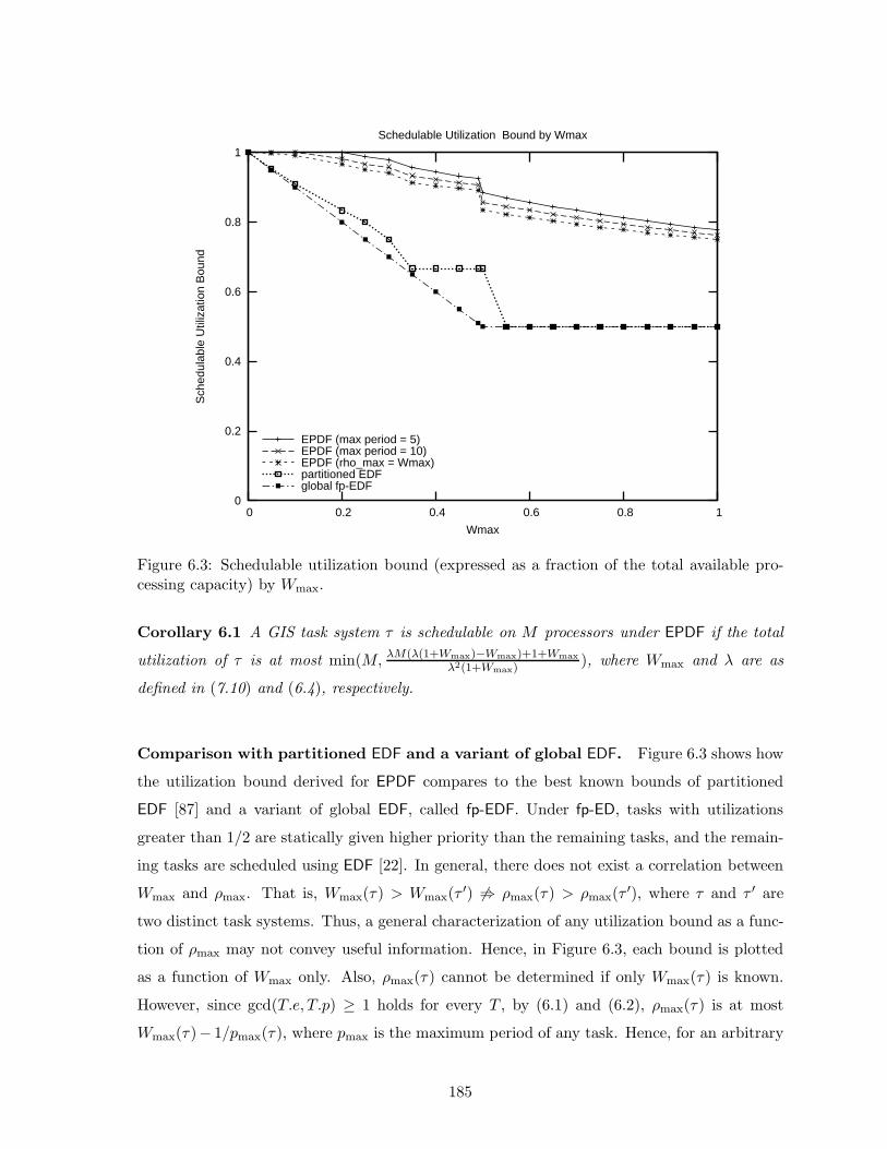
0

0.2

0.4

0.6

0.8

1

0 0.2 0.4 0.6 0.8 1

Sch

edul

able

Util

izat

ion

Bou

nd

Wmax

Schedulable Utilization Bound by Wmax

EPDF (max period = 5)EPDF (max period = 10)EPDF (rho_max = Wmax)partitioned EDFglobal fp-EDF

Figure 6.3: Schedulable utilization bound (expressed as a fraction of the total available pro-cessing capacity) by Wmax.

Corollary 6.1 A GIS task system τ is schedulable on M processors under EPDF if the total

utilization of τ is at most min(M, λM(λ(1+Wmax)−Wmax)+1+Wmax

λ2(1+Wmax)), where Wmax and λ are as

defined in (7.10) and (6.4), respectively.

Comparison with partitioned EDF and a variant of global EDF. Figure 6.3 shows how

the utilization bound derived for EPDF compares to the best known bounds of partitioned

EDF [87] and a variant of global EDF, called fp-EDF. Under fp-ED, tasks with utilizations

greater than 1/2 are statically given higher priority than the remaining tasks, and the remain-

ing tasks are scheduled using EDF [22]. In general, there does not exist a correlation between

Wmax and ρmax. That is, Wmax(τ) > Wmax(τ′) 6⇒ ρmax(τ) > ρmax(τ

′), where τ and τ ′ are

two distinct task systems. Thus, a general characterization of any utilization bound as a func-

tion of ρmax may not convey useful information. Hence, in Figure 6.3, each bound is plotted

as a function of Wmax only. Also, ρmax(τ) cannot be determined if only Wmax(τ) is known.

However, since gcd(T.e, T.p) ≥ 1 holds for every T , by (6.1) and (6.2), ρmax(τ) is at most

Wmax(τ)− 1/pmax(τ), where pmax is the maximum period of any task. Hence, for an arbitrary

185

task system, a utilization bound higher than that given by min(M,U(M,λ,Wmax)) is possible if

at least pmax is also known. Thus, in Figure 6.3, utilization bounds for EPDF for tasks systems

with pmax = 5 and pmax = 10 computed using Theorem 6.1 assuming ρmax = Wmax−1/pmax are

plotted, as is the U(M,λ,Wmax) bound. As can be seen from the plots, the utilization bound

of EPDF is higher than those of the other two algorithms by around 25% in the worst case.

Also, the utilization bound of EPDF is piece-wise continuous with discontinuities whenever λ

changes, i.e., at Wmax = 1/p, where p is an integer.

In [107], Srinivasan and Anderson have shown that EPDF can correctly schedule every task

system with Wmax ≤ 1M−1 . With Wmax = 1

M−1 , the utilization bound given by Corollary 6.1

is M − 1M−1 + 1

(M−1)2 , which approaches M asymptotically. The discrepancy for lower values

of M is due to the approximation of ρmax by Wmax. Hence, the results of this paper are useful

only when Wmax > 1M−1 holds.

How accurate is the utilization bound given by Theorem 6.1? Is it the worst-case for EPDF?

As yet, we do not fully know the answers to these questions. The closest we have come towards

providing any answer is the following task system, which can miss deadlines under EPDF.

Counterexample. Consider a task system that consists of 2n+1 tasks of weight 12 , n tasks of

weight 34 , and n tasks of weight 5

6 scheduled on 3n processors, where n ≥ 2. There is an EPDF

schedule for this task system in which a deadline miss occurs at time 12. One such schedule

is shown in Figure 6.4. The total utilization of this task system is 31n12 + 1

2 , which approaches

86.1% of 3n, the total processing capacity, as n approaches infinity. The utilization bound

given by Theorem 6.1 for a task system with task parameters as in this example is slightly

above 80% for large M . Hence, at least asymptotically, the value derived does not seem to

be too pessimistic. However, the same cannot be said when M is small. For instance, for the

example under consideration, the total utilizations when n = 2 and n = 3 (i.e., M = 6 and

M = 9) are 94.4% and 91.6%, respectively, while the estimated values are only 84.1% and

82.7%. Further, though this single task system is too little data to draw general conclusions,

the difficulty in identifying counterexamples and some of the approximations made in the

analysis make us strongly believe that our result is not tight.

186

z { | } ~ � � � � � {z {{ {|

�|��{��|��{

��{��{{

�

��

�

�

��

��

�

��

��

|��{|� { |�

|� � ��{

��{ {

��

{ {

�{�

|

��}�

��

��

��

Figure 6.4: An EPDF schedule with a deadline miss for a task system with 2n + 1 tasks ofweight 1

2 , n tasks with weight 34 , and n tasks with weight 5

6 on M = 3n processors, wheren ≥ 2. The number of tasks for each weight scheduled in each time slot is indicated. Asn → ∞, the total utilization of this task system approaches 86.1%.

6.3 Summary

We have determined a utilization bound for the non-optimal earliest-pseudo-deadline-first

(EPDF) Pfair scheduling algorithm on multiprocessors, and thereby, presented a sufficient

schedulability test for EPDF. In general, on M > 2 processors, the utilization bound derived is

at least 3M+14 , and is higher than that of every non-Pfair algorithm by around 25% when task

utilizations are not restricted. Our bound is expressed as a decreasing function of the maxi-

mum weight, Wmax, of any task, and hence, if this value is known, may be used to schedule

task systems with total utilization exceeding 3M+14 . A knowledge of EPDF’s utilization bound

should help in identifying the task systems for which the soft real-time scheduling results of

EPDF are applicable. Also, if the total utilization of an EPDF-scheduled soft real-time system

is less than the schedulable utilization bound of EPDF, then that system can be treated as a

hard real-time system.

Currently, it is not known whether the utilization bound derived is a worst-case schedulable

utilization for EPDF. We have only presented a counterexample that shows that the worst-case

value for Wmax ≤ 56 is at most 86.1%, which also suggests that a significant improvement to

the result may not be likely. Towards the end of the next chapter, we extend this result to

187

allow non-zero tardiness.

188

Chapter 7

Improved Conditions for Bounded

Tardiness under EPDF1

In this chapter, we present results concerning EPDF that can enable its use with more soft

real-time systems than previously possible. Our contributions are as follows.

As mentioned in Chapter 6, the efficacy of EPDF for soft real-time systems was first consid-

ered by Srinivasan and Anderson in [106]. They conjectured that on M processors, EPDF can

ensure a tardiness bound of one quantum to every task system with total utilization at most

M (i.e., every task system that is feasible on M processors). Our first result in this chapter

refutes this conjecture. For this, we present counterexamples that show that tardiness under

EPDF can not only exceed one quantum, but can be up to four quanta. The method used

to generate these counterexamples suggests that, in general, EPDF cannot guarantee small

constant tardiness that is independent of the task system parameters.

In [106], Srinivasan and Anderson showed that EPDF can guarantee a tardiness bound of

q ≥ 1 quanta for every ‘ subtask of a feasible task system, provided a certain condition holds.

Their condition can be ensured by limiting each task’s weight to at most qq+1 . As a second

contribution, we improve upon this result, and show that a more liberal restriction of q+2q+3 on

the weight of each task is sufficient to ensure that tardiness does not exceed q quanta. Note

that, when q = 1, our result presents an improvement of 50% over the previous result.

As a third contribution, we present a sufficient restriction of Udef=

1Contents of this chapter previously appeared in preliminary form in the following paper:[48] U. Devi and J. Anderson. Improved conditions for bounded tardiness under EPDF fair multiprocessorscheduling. In Proceedings of the 12th International Workshop on Parallel and Distributed Real-Time Systems,April 2004. 8 pages (on CD-ROM).

min(M, ((q+1)Wmax+(q+2))M+((2q+1)Wmax+1)2(q+1)Wmax+2 ) on the total utilization of a task system for

ensuring a tardiness bound of q ≥ 1 quanta on M processors, for task systems whose

maximum task weight may exceed q+2q+3 . For q = 1, U is around 83.5%, which is higher by

around 8% over that presented in the previous chapter for hard real-time systems.

The results described above are presented in order in Sections 7.1, 7.2, and 7.3. Section 7.4

concludes.

7.1 Counterexamples

It is easy to show that subtask deadlines can be missed under EPDF. In [106], it was conjectured

that EPDF ensures a tardiness bound of one for every feasible task system. We now show that

this conjecture is false.

Theorem 7.1 Tardiness under EPDF can exceed three quanta for feasible GIS task systems.

In particular, if EPDF is used to schedule task system τ (i) (1 ≤ i ≤ 3) in Table 7.1, then a

tardiness of i + 1 quanta is possible.

Proof: Figure 7.1 shows a schedule for τ (1), in which a subtask has a tardiness of two at time

50. The schedules for τ (2) and τ (3) are too lengthy to be depicted; we verified them using two

independently-coded EPDF simulators. �

7.2 Tardiness Bounds for EPDF

In this section, we present results concerning tardiness bounds that can be guaranteed under

EPDF. The sufficient condition for a tardiness of q ≥ 1 quanta as given by Srinivasan and

Anderson in [106] requires that the sum of the weights of the M −1 heaviest tasks be less than

qM+1q+1 . This can be ensured if the weight of each task is restricted to be at most q

q+1 . We next

show that an improved weight restriction of q+2q+3 per task is sufficient to guarantee a tardiness

of q quanta. This restriction is stated below.

(W) The weight of each task in the task system under consideration is at most

q+2q+3 .

In what follows, we prove the following theorem.

Theorem 7.2 Tardiness under EPDF is at most q quanta, where q ≥ 1, for every GIS task

system that is feasible on M ≥ 3 processors and that satisfies (W ).

190

0 8 16 24 32 40 48

33

66

66

4 24 2

4

4 2

2

2 4

2 4

2 42 4

66

66

66

66

6

4 24 2

2 42 4

2 42 4

66

66

66

66

66

66

66

66

5 1

33

3

33

3

33

3

33

3

33

1 2

2 12 1

3

33

3

33

3

33

1 2

2 12 1

3 3

33

3

4 41 3

41 3

41 3

41 3

2 21 3

1 31 3

41 3

41 3

2 21 3

1 31 1

41 1 2

21

2

3

33

44 tasks ofweight 1/2



Figure 7.1: Counterexample to prove that tardiness under EPDF can exceed one quantum. 13periodic tasks with total utilization ten are scheduled on ten processors. In the schedule, tasksof the same weight are shown together as a group. Each column corresponds to a time slot.The PF-window of each subtask is shown as a sequence of dashes that are aligned. An integervalue n in slot t means that n tasks in the corresponding group have a subtask scheduled att. Subtasks that miss deadlines are shown scheduled after their windows. Ties are broken infavor of tasks with lower weights. In this schedule, 11 subtasks miss their deadlines at time48. Hence, tardiness is 2 quanta for at least one subtask.

To prove the above theorem, we use a setup similar to that used by Srinivasan and Anderson

in [105] and [106] (which was also used in Chapter 6). (Again, it should be pointed out that

the details of the current proof differ significantly from the rest.) As in Chapter 6, our proof is

by contradiction. Hence, we assume that Theorem 7.2 does not hold, and as before, we define

a task system that is minimal in some sense for which the theorem to be proved does not hold.

Thus, for the problem at hand, our assumption implies that there exists a q ≥ 1, and a time

td and a concrete task system σ defined as follows.

Definition 7.1: td is the earliest deadline of a subtask with a tardiness of q + 1 under EPDF

in any feasible GIS task system satisfying (W), i.e., there exists some such task system with a

subtask with deadline at td and tardiness q + 1, and there does not exist any such task system

with a subtask with deadline prior to td and a tardiness of q + 1.

Definition 7.2: σ is a feasible concrete GIS task system satisfying (W) with the following

properties.

(S1) A subtask in σ with deadline at td has a tardiness of q + 1 under EPDF.

(S2) No feasible concrete task system satisfying (W) and (S1) releases fewer subtasks in [0, td)

than σ.

191

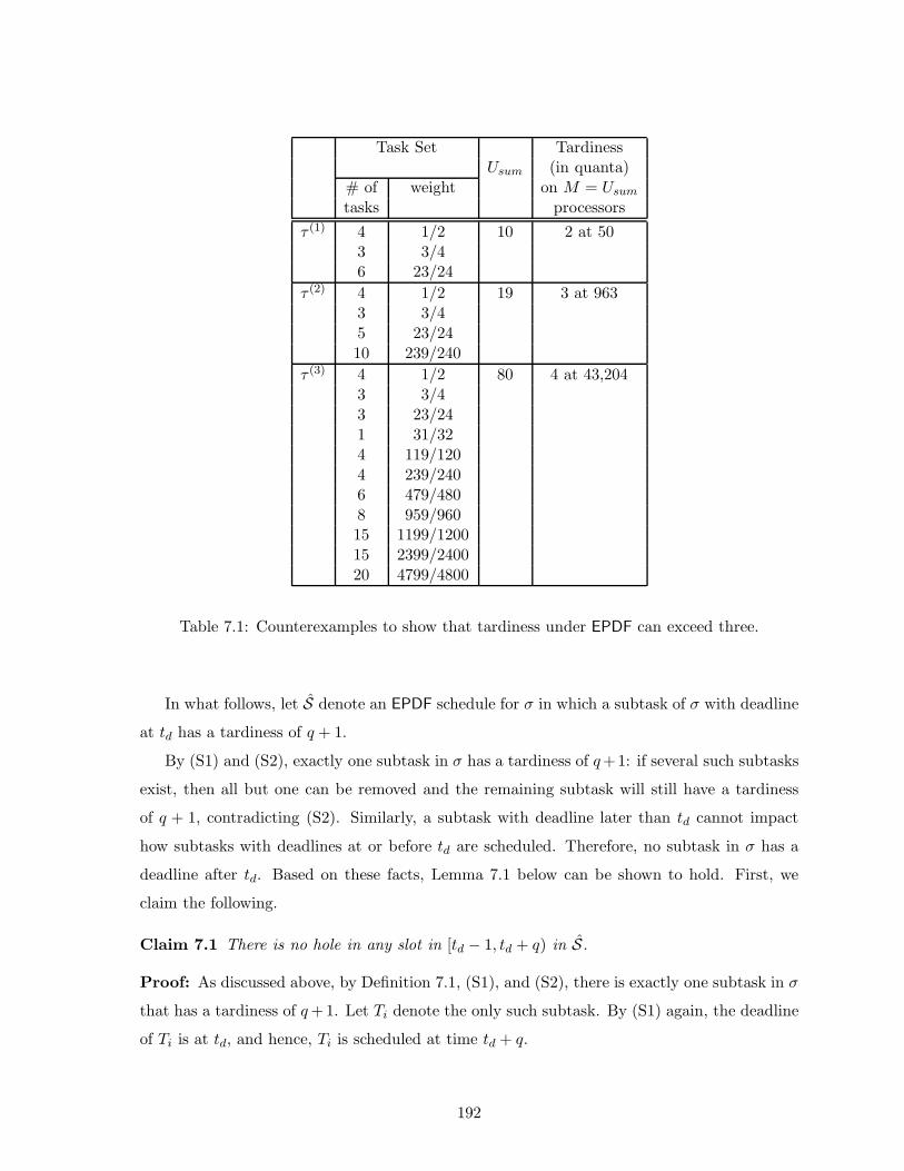
Task Set TardinessUsum (in quanta)

# of weight on M = Usum

tasks processors

τ (1) 4 1/2 10 2 at 503 3/46 23/24

τ (2) 4 1/2 19 3 at 9633 3/45 23/2410 239/240

τ (3) 4 1/2 80 4 at 43,2043 3/43 23/241 31/324 119/1204 239/2406 479/4808 959/96015 1199/120015 2399/240020 4799/4800

Table 7.1: Counterexamples to show that tardiness under EPDF can exceed three.

In what follows, let S denote an EPDF schedule for σ in which a subtask of σ with deadline

at td has a tardiness of q + 1.

By (S1) and (S2), exactly one subtask in σ has a tardiness of q +1: if several such subtasks

exist, then all but one can be removed and the remaining subtask will still have a tardiness

of q + 1, contradicting (S2). Similarly, a subtask with deadline later than td cannot impact

how subtasks with deadlines at or before td are scheduled. Therefore, no subtask in σ has a

deadline after td. Based on these facts, Lemma 7.1 below can be shown to hold. First, we

claim the following.

Claim 7.1 There is no hole in any slot in [td − 1, td + q) in S.

Proof: As discussed above, by Definition 7.1, (S1), and (S2), there is exactly one subtask in σ

that has a tardiness of q +1. Let Ti denote the only such subtask. By (S1) again, the deadline

of Ti is at td, and hence, Ti is scheduled at time td + q.

192

The proof of the claim is by induction on decreasing time t. We start by showing that

there is no hole in slot td + q − 1.

Base Case: t = td + q − 1. Let Th denote the predecessor, if any, of Ti. Because the

deadlines of any two successive subtasks of the same task differ by at least one time unit,

d(Th) ≤ td − 1 holds. Therefore, by Definition 7.1, the tardiness of Th is at most q, and Th

completes executing by td + q−1. Hence, no subtask of T is scheduled in slot td + q−1. Thus,

there is no hole in slot td + q − 1; otherwise, EPDF would schedule Ti there.

Induction Hypothesis: Assume that there is no hole in slots [t′, td + q), where td − 1 <

t′ < td + q.

Induction Step: t = t′ − 1. We show that there is no hole in slot t′ − 1. The deadline

of every subtask scheduled in t′ is at most td. Hence, the release time and the eligibility time

of every such subtask is at or before td − 1. Since td − 1 ≤ t′ − 1, every subtask scheduled

at t′ can be scheduled at t′ − 1 unless its predecessor is scheduled at t′ − 1. By the induction

hypothesis, there is no hole in slot t′. Hence, if there is a hole in t′ − 1, then at most M − 1 of

the M subtasks scheduled at t′ can have their predecessors scheduled at t′ − 1, implying that

at least one of the subtasks scheduled at t′ should have been scheduled at t′ − 1, which is a

contradiction. Therefore, there can be no hole in t′ − 1. �

We now show that LAG of σ at td is exactly qM + 1.

Lemma 7.1 LAG(σ, td, S) = qM + 1.

Proof: By Claim 7.1, there is no hole in any slot in [td, td + q) in S. Further, the subtask

with a tardiness of q + 1 and deadline at td, as specified in (S1), is not scheduled until time

td + q. (Also, recall that there is exactly one such subtask.) Thus, because every subtask in

σ has a deadline of at most td, there exist exactly qM + 1 subtasks with deadlines at most td

that are pending at td in S. In the ideal schedule, all of these subtasks complete executing by

time td. Therefore, the LAG of σ at td, which is the difference between the ideal allocation and

the allocation in S in [0, td), is qM + 1. �

By Claim 7.1, there is no hole in slot td−1. Therefore, by the contrapositive of Lemma 3.4,

LAG(σ, td−1, S) ≥ LAG(σ, td, S), which, by Lemma 7.1, is qM+1. Thus, because LAG(σ, 0, S) =

0, there exists a time t, where 0 ≤ t < td − 1 such that LAG(σ, t, S) < qM + 1 and

193

LAG(σ, t + 1, S) ≥ qM + 1. This further implies the existence of a time 0 ≤ th < td − 1,

a concrete task system τ , and an EPDF schedule S for τ defined as follows.

Definition 7.3: 0 ≤ th < td − 1 is the earliest time such that the LAG in any EPDF schedule

for any feasible concrete GIS task system satisfying (W) is at least qM + 1 at th + 1.

Definition 7.4: τ is a feasible concrete GIS task system satisfying (W) with the following

properties.

(T1) LAG(τ, th + 1,S) ≥ qM + 1.

(T2) No feasible concrete task system satisfying (W) and (T1) releases fewer subtasks than τ .

(T3) No feasible concrete task system satisfying (W), (T1), and (T2) has a larger rank than

τ where the rank of a task system is the sum of the eligibility times of all its subtasks, i.e.,

rank(τ, t) =∑

{Ti∈τ} e(Ti).

(T2) can be thought of as identifying a minimal task system in the sense of having LAG

exceed qM + 1 at the earliest possible time with the fewest number of subtasks, subject

to satisfying (W). As already explained, if Theorem 7.2 does not hold for all task systems

satisfying (W), then there exists some task system whose LAG is at least qM + 1. Therefore,

some task system satisfying (W), (T1), and (T2) necessarily exists. (T3) further restricts the

nature of such a task system by requiring subtask eligibility times to be spaced as much apart

as possible.

Before continuing with the proof, we would like to point out the following as we did in

Chapter 6. As mentioned earlier, the overall proof setup here is similar to that used in [105]

for establishing the optimality of the PD2 algorithm, and in Chapter 6 for determining a

schedulable utilization bound for EPDF. Though the details of the proofs differ significantly,

some basic properties hold for the task systems considered in each problem, such as task

system τ in Definition 7.4. The proofs of some such basic properties may have to be reworded

to exactly hold for the task system under consideration. However, to avoid repetition, we

simply borrow such properties without proof, but explicitly state that when we have done so.

We next prove some properties about the subtasks of τ scheduled in S.

Lemma 7.2 Let Ti be a subtask in τ . Then, the following properties hold.

(a) If Ti is scheduled at t, then e(Ti) ≥ min(r(Ti), t).

(b) If Ti is scheduled before td, then tardiness of Ti is at most q.

194

Proof of part (a): The proof for this part is very similar to that of Lemma 6.8(d), but

is provided to give a flavor of the changes in wording needed to fit the task system under

consideration here. Suppose e(Ti) is not equal to min(r(Ti), t). Then, by (3.12) and because

Ti is scheduled at t, it is before min(r(Ti), t). Hence, simply changing e(Ti) so that it equals

min(r(Ti), t) will not affect how Ti or any other subtask is scheduled. That is, the actual allo-

cations in S to every task, and hence, the lag of every task, will remain unchanged. Therefore,

the LAG of τ at th + 1 will still be at least qM + 1. However, changing the eligibility time of

Ti increases the rank of the task system, and hence, (T3) is contradicted. �

Proof of part (b). Follows from Definition 7.1. �

In what follows, we show that if (W) is satisfied, then there does not exist a time th as defined

in Definition 7.3, that is, we contradict its existence, and in turn prove Theorem 7.2. For this,

we deduce the LAG of τ at th + 1 by determining the lags of the tasks in τ .

By the definition there of th in Definition 7.3, LAG(τ, th + 1) > LAG(τ, th). Hence, by

Lemma 3.4, the following holds.

(H) There is at least one hole in slot th.

7.2.1 Categorization of Subtasks

As can be seen from (3.22) and (3.15), the lag of a task T at t depends on the allocations that

subtasks of T receive in each time slot until t in the ideal schedule. Hence, a tight estimate of

such allocations is essential to bounding the lag of T reasonably accurately. If a subtask’s index

is not known, then (3.15), which can otherwise be used to compute the allocation received by

any subtask in any slot exactly , is not of much help. Hence, in this subsection, we define terms

that will help in categorizing subtasks, and then derive upper bounds for the allocations that

these categories of subtasks receive in the ideal schedule.

k-dependent subtasks. The subtasks of a heavy task with weight in the range [1/2, 1) can

be divided into “groups” based on their group deadlines in a straightforward manner: place

all subtasks with identical group deadlines in the same group and identify the group using

the smallest index of any subtask in that group. For example, in Figure 3.5, G1 = {T1, T2},G3 = {T3, T4, T5}, and G6 = {T6, T7, T8}. If there are no IS separations or GIS omissions among

the subtasks of a group, then a deadline miss by q quanta for a subtask Ti will necessarily

195

result in a deadline miss by at least q quanta for the remaining subtasks in Ti’s group. Hence,

a subtask Tj is dependent on all prior subtasks in its group for not missing its deadline. If

T is heavy, we say that Tj is k-dependent, where k ≥ 0, if Tj is the (k + 1)st subtask in

its group, computed assuming all subtasks are present (that is, as in the determination of

group deadlines, even if T is GIS and some subtasks are omitted, k-dependency is determined

assuming there are no omissions).

Recall that by Lemma 3.1 all subtasks of a heavy task with weight less than one are of

length two or three. Further, note that each subtask in each group except possibly the first is

of length two. This implies that for a periodic task the deadlines of any two successive subtasks

that belong to the same group differ by exactly one. Also, each subtask in each group except

possibly the final subtask has a b-bit of one. Finally, if the final subtask of a group has a b-bit

of one, then the first subtask of the group that follows in of length three. These properties are

summarized in the following three lemmas.

Lemma 7.3 Let T be a heavy task with wt(T ) < 1 and let Ti be a 0-dependent subtask of T .

Then, one of the following holds: (i) i = 1; (ii) i > 1 and b(Ti−1) = 0; (iii) |ω(Ti)| = 3.

Lemma 7.4 If Ti is a k-dependent subtask of a periodic task T , where i ≥ 2 and k ≥ 1, then

d(Ti) = d(Ti−1) + 1 and r(Ti) = d(Ti−1) − 1.

Lemma 7.5 Let Ti, where i > 1, be a k-dependent subtask of T with wt(T ) < 1. If k ≥ 1,

then |ω(Ti)| = 2 and b(Ti−1) = 1.

If a task T is light, then we simply define all of its subtasks to be 0-dependent. In this

case, each subtask is in its own group.

Miss initiators. A subtask scheduled at t and missing its deadline by c quanta, where

c ≥ 1, is referred to as a miss initiator by c (or a c-MI, for short) for its group, if no subtask

of the same task is scheduled at t − 1. (A miss initiator by q, i.e., a q-MI, will simply be

referred to as an MI.) Thus, a subtask is a c-MI if it misses its deadline by c quanta and is

either the first subtask in its group to do so or is separated from its predecessor by an IS or

GIS separation, and its predecessor is not scheduled in the immediately preceding slot. Such a

subtask is termed a miss initiator by c because in the absence of future separations, it causes all

subsequent subtasks in its group to miss their deadlines by c quanta as well. Several examples

of MIs for q = 1 are shown in Figure 7.2.

196

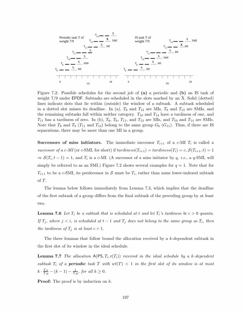
9 18

T

T

T

T

T

T

T8

9

10

11

12

13

14

X

X

X

X

XX

X

MI

MI

9

T8

X MI

X

T

T

T

9

10

11

X

X

MI

T

T

13

14XX

X

MI

MI

20 (a) (b)

X

SMI

SMI

SMI

SMIweight 7/9Periodic task T of

weight 7/9IS task T of

Figure 7.2: Possible schedules for the second job of (a) a periodic and (b) an IS task ofweight 7/9 under EPDF. Subtasks are scheduled in the slots marked by an X. Solid (dotted)lines indicate slots that lie within (outside) the window of a subtask. A subtask scheduledin a dotted slot misses its deadline. In (a), T8 and T12 are MIs, T9 and T13 are SMIs, andthe remaining subtasks fall within neither category. T10 and T14 have a tardiness of one, andT11 has a tardiness of zero. In (b), T8, T9, T11, and T13 are MIs, and T10 and T14 are SMIs.Note that T8 and T9 (T11 and T13) belong to the same group G8 (G11). Thus, if there are ISseparations, there may be more than one MI in a group.

Successors of miss initiators. The immediate successor Ti+1 of a c-MI Ti is called a

successor of a c-MI (or c-SMI, for short) if tardiness(Ti+1) = tardiness(Ti) = c, S(Ti+1, t) = 1

⇒ S(Ti, t − 1) = 1, and Ti is a c-MI. (A successor of a miss initiator by q, i.e., a q-SMI, will

simply be referred to as an SMI.) Figure 7.2 shows several examples for q = 1. Note that for

Ti+1 to be a c-SMI, its predecessor in S must be Ti, rather than some lower-indexed subtask

of T .

The lemma below follows immediately from Lemma 7.3, which implies that the deadline

of the first subtask of a group differs from the final subtask of the preceding group by at least

two.

Lemma 7.6 Let Ti be a subtask that is scheduled at t and let Ti’s tardiness be c > 0 quanta.

If Tj , where j < i, is scheduled at t − 1 and Tj does not belong to the same group as Ti, then

the tardiness of Tj is at least c + 1.

The three lemmas that follow bound the allocation received by a k-dependent subtask in

the first slot of its window in the ideal schedule.

Lemma 7.7 The allocation A(PS, Ti, r(Ti)) received in the ideal schedule by a k-dependent

subtask Ti of a periodic task T with wt(T ) < 1 in the first slot of its window is at most

k · T.eT.p − (k − 1) − 1

T.p , for all k ≥ 0.

Proof: The proof is by induction on k.

197

Base Case: k = 0. Because wt(T ) < 1, and T.e and T.p are integral, T.e ≤ T.p − 1. Thus,

by (3.18), A(PS, Ti, r(Ti)) ≤ wt(T ) ≤ 1 − 1/T.p, and the lemma holds for the base case.

Induction Step: Assuming that the lemma holds for (k − 1)-dependent subtasks, we show

that it holds for k-dependent subtasks, where k ≥ 1. Because k ≥ 1, by the definition of

k-dependency, i > 1 and T is heavy. Hence, by Lemma 3.1, |ω(Ti−1)| is either two or three.

We consider two cases.

Case 1: |ω(Ti−1)| = 2. Since k ≥ 1, Ti−1 is (k − 1)-dependent. Therefore, by the induction

hypothesis,

A(PS, Ti−1, r(Ti−1)) ≤ (k − 1) · (T.e/T.p) − (k − 2) − (1/T.p). (7.1)

Because |ω(Ti−1)| = 2, by (3.17), A(PS, Ti−1, d(Ti−1) − 1) = 1 − A(PS, Ti−1, r(Ti−1)). Hence,

by (7.1), A(PS, Ti−1, d(Ti−1) − 1) ≥ (k − 1) + (1/T.p) − (k − 1) · (T.e/T.p). Because Ti is

k-dependent, where k ≥ 1, by Lemma 7.5, b(Ti−1) = 1, and by Lemma 3.3, A(PS, Ti, r(Ti)) =

(T.e/T.p) − A(PS, Ti−1, d(Ti−1) − 1) ≤ k · (T.e/T.p) − (k − 1) − (1/T.p).

Case 2: |ω(Ti−1)| = 3. By Lemma 7.5, Ti−1 is 0-dependent; hence, Ti is 1-dependent, i.e.,

k = 1. By Lemma 7.5, b(Ti−1) = 1, and hence, by Lemma 3.3,

A(PS, Ti, r(Ti)) =T.e

T.p− A(PS, Ti, d(Ti−1) − 1) ≤ T.e

T.p− 1

T.p(by 3.19). �

Lemma 7.8 The allocation A(PS, Ti, r(Ti)) received in the ideal schedule by a k-dependent

subtask Ti of a GIS task T in the first slot of its window is at most k · T.eT.p − (k − 1) − 1

T.p .

Proof: Follows from Lemma 7.7 and the definition of GIS tasks. (The allocation that Ti

receives in each slot of its window is identical to the allocation that it would receive if T were

periodic.) �

Lemma 7.9 Let Ti, where i ≥ k + 1 and k ≥ 1, be a subtask of T with wt(T ) < 1 such that

|ω(Ti)| ≥ 3 and b(Ti−1) = 1. Let the number of subtasks in Ti−1’s dependency group be at least

k. Then, A(PS, Ti, r(Ti)) ≤ k · T.eT.p − (k − 1) − 1

T.p .

Proof: Since |ω(Ti)| ≥ 3, by Lemma 7.5, Ti is 0-dependent and is the first subtask in its group.

Hence, Ti−1 is the final subtask in its dependency group, and since there are at least k subtasks

198

in Ti−1’s group, Ti−1 is (k − 1)-dependent. Hence, by Lemma 7.8, A(PS, Ti−1, r(Ti−1)) ≤(k−1) · T.e

T.p − (k−2)− 1T.p . (What follows is similar to the reasoning used in the induction step

in Lemma 7.7.) If |ω(Ti−1)| = 2, then, by (3.17), A(PS, Ti−1, d(Ti−1)) ≥ 1− ((k−1) · T.eT.p − (k−

2)− 1T.p) = (k−1)− (k−1) · T.e

T.p + 1T.p . By the statement of the lemma, b(Ti−1) = 1, and hence,

by Lemma 3.3, A(PS, Ti, r(Ti)) = wt(T ) − A(PS, Ti−1, d(Ti−1) − 1) ≤ k · T.eT.p − (k − 1) − 1

T.p .

Thus, the lemma holds when |ω(Ti−1)| = 2.

On the other hand, if |ω(Ti−1)| ≥ 3, then by Lemma 7.5, Ti−1 is 0-dependent. By

(3.19), A(PS, Ti−1, d(Ti−1) − 1) ≥ 1T.p , and hence, because b(Ti−1) = 1, by Lemma 3.3,

A(PS, Ti, r(Ti)) = wt(T ) − A(PS, Ti−1, d(Ti−1) − 1) ≤ T.eT.p − 1

T.p . By the statement of the

lemma, |ω(Ti)| = 3, and hence, Ti is also 0-dependent. Thus, Ti−1 is the only subtask in its

group, and hence, k = 1. (Note that k here denotes the number of subtasks that are in the

same dependency group as Ti−1.) Therefore, the lemma holds for this case too. �

Having determined a bound on the allocation received by a subtask in the first slot of its

window in the ideal schedule based on its k-dependency, we next bound the lag of a task at

time t, this time based on the k-dependency of its last-scheduled subtask.

Lemma 7.10 Let Ti be a k-dependent subtask of a task T for k ≥ 0, and let the tardiness of

Ti be s for some s ≥ 1 (that is, Ti is scheduled at time d(Ti)+ s− 1). Then lag(T, d(Ti)+ s) <

(k + s + 1) · wt(T ) − k.

Proof: By the statement of the lemma, Ti and all prior subtasks of T are scheduled in

[0, d(Ti)+s). Hence, lag(T, d(Ti)+s) depends on the number of subtasks of T after Ti released

prior to d(Ti)+s, the allocations they receive in the ideal schedule, and when they are scheduled

in S. It can be verified from (3.9), (3.10), and (3.8) that at most s + 1 successors of Ti —

Ti+1, . . . , Ti+s+1 — are released before d(Ti) + s. Hence, the lag of T at d(Ti) + s in S is

maximized if all those subtasks are present and are released without any IS separations and

S has not scheduled any of them by time d(Ti) + s. We will assume that this is the case. By

Lemma 6.10, at most one successor of Ti, namely Ti+1, can have a release time that is before

d(Ti). Further, r(Ti+1) ≥ d(Ti) − 1 holds. Hence, lag(T, d(Ti) + s) ≤ A(PS, Ti+1, d(Ti) − 1)) +

A(PS, T, d(Ti), d(Ti) + s). If r(Ti+1) > d(Ti) − 1 holds, then A(PS, Ti+1, d(Ti) − 1) = 0. On

the other hand, if r(Ti+1) = d(Ti) − 1, then by (3.6), b(Ti) = 1. Further, either |ω(Ti+1)| = 2

or |ω(Ti+1)| > 2. In the former case, T is heavy, and by the definition of k-dependency, Ti+1

belongs to the same dependency group as Ti and is (k + 1)-dependent. Hence, by Lemma 7.8,

A(PS, Ti+1, r(Ti+1)) ≤ (k + 1) · wt(T ) − k − 1T.p . If the latter holds, i.e., |ω(Ti+1)| > 2,

199

we reason as follows. Since Ti is k-dependent, the number of subtasks in Ti’s group is at

least k + 1. Therefore, since b(Ti) = 1, Lemma 7.9 applies for Ti+1 and it follows that

A(PS, Ti+1, r(Ti+1)) ≤ (k + 1) · wt(T ) − k − 1T.p . Thus, in either case, A(PS, Ti+1, d(Ti) − 1) =

A(PS, Ti+1, r(Ti+1)) ≤ (k + 1) · wt(T ) − k − 1T.p .

By (3.16), A(PS, T, d(Ti), d(Ti)+s) ≤ s·wt(T ). Hence, lag(T, d(Ti)+s) ≤ A(PS, Ti+1, d(Ti)−1)) + A(PS, T, d(Ti), d(Ti) + s) ≤ (k + s + 1) · wt(T ) − k − 1

T.p < (k + s + 1) · wt(T ) − k. �

7.2.2 Subclassification of Tasks in A(t)

Recall from Section 3.6 that a task in A(t) is scheduled in slot t. We further classify tasks in

A(t), based on the tardiness of their subtasks scheduled at t, as follows.

A0(t): Includes T in A(t) iff its subtask scheduled at t has zero tardiness.

Aq(t): Includes T in A(t) iff its subtask scheduled at t has a tardiness of q.

Aq−1(t), q > 1: Includes T in A(t) iff its subtask scheduled at t has a tardiness greater than 0

and less than q.

Aq(t) is further partitioned into A0q(t), A1

q(t), and A2q(t).

A0q(t): Includes T in Aq(t) iff its subtask scheduled at t is an MI.

A1q(t): Includes T in Aq(t) iff its subtask scheduled at t is an SMI.

A2q(t): Includes T in Aq(t) iff its subtask scheduled at t is neither an MI nor an SMI.

A0q−1(t), q > 1: Includes T in Aq−1(t) iff its subtask scheduled at t is a c-MI, where 0 < c < q.

From the above, we have the following.

A0(t) ∪ Aq(t) ∪ Aq−1(t) = A(t) and A0q(t) ∪ A1

q(t) ∪ A2q(t) = Aq(t) (7.2)

A0(t) ∩ Aq(t) = Aq(t) ∩ Aq−1(t) = Aq−1(t) ∩ A0(t) = ∅ (7.3)

A0q(t) ∩ A1

q(t) = A1q(t) ∩ A2

q(t) = A2q(t) ∩ A0

q(t) = ∅ (7.4)

7.2.3 Task Lags by Task Classes and Subclasses

The next eight lemmas give bounds on the lags of tasks in A(t), B(t), and I(t) at t + 1,

where t ≤ th is a slot with a hole, and hence, hold for th, as well. As mentioned earlier, some

of these lemmas are proved for a slightly different task system, but hold for τ as defined here

in Definition 7.4 as well.

Let t ≤ th be a slot with a hole. Then, Lemmas 7.11–7.18 hold.

200

Lemma 7.11 (from [106]) For T ∈ I(t), lag(I, t + 1) = 0.

Lemma 7.12 (from Chapter 6) For T ∈ B(t), lag(B, t + 1) = 0.

Lemma 7.13 (from Chapter 6) For T ∈ A0(t), 0 ≤ lag(T, t + 1) < wt(T ).

Lemma 7.14 For T ∈ A0q(t), lag(T, t + 1) < (q + 1) · wt(T ).

Proof: If T ∈ A0q(t), then the subtask Ti of T scheduled at t is an MI, and d(Ti) = t − q + 1.

Further Ti is k-dependent, where k ≥ 0. Hence, by Lemma 7.10, lag(T, t + 1) is less than

((k + q +1) ·wt(T )− k), which (because wt(T ) ≤ 1) is at most (q +1) ·wt(T ), for all k ≥ 0. �

The two lemmas below follow similarly.

Lemma 7.15 For T ∈ A1q(t), lag(T, t + 1) < (q + 2) · wt(T ) − 1.

Proof: If T ∈ A1q(t), then the subtask Ti of T scheduled at t is an SMI, and is k-dependent for

k ≥ 1. Also, d(Ti) = t− q + 1. Thus, by Lemma 7.10, lag(T, t + 1) < (k + q + 1) ·wt(T )− k ≤(q + 2) · wt(T ) − 1 for all k ≥ 1 (because wt(T ) ≤ 1). �

Lemma 7.16 For T ∈ A2q(t), lag(T, t + 1) < (q + 3) · wt(T ) − 2.

Proof: Similar to that of Lemma 7.15. �

Lemma 7.17 For T ∈ Aq−1(t), lag(T, t + 1) < q · wt(T ).

Proof: Let Ti be T ’s subtask scheduled at t and let s denote the tardiness of Ti. Then,

t + 1 = d(Ti) + s. Let Ti be k-dependent, where k ≥ 0. By the definition of Aq−1, 0 < s < q

holds, and by Lemma 7.10, lag(T, d(Ti) + s) = lag(T, t + 1) < (k + s + 1) · wt(T ) − k ≤(k + q) · wt(T ) − k ≤ q · wt(T ), for all k ≥ 0. �

Lemma 7.18 For T ∈ A(t), lag(T, t + 1) ≥ 0.

Proof: If T is in A0(t), then the lemma follows from Lemma 7.13. Otherwise, T ’s subtask

scheduled at t has non-zero tardiness. Hence, T could not have received more allocation in Sthan in the ideal schedule. �

201

7.2.4 Some Auxiliary Lemmas

In proving Theorem 7.2, we make use of Lemmas 6.3, 6.4, and 6.5 established in prior work

by Srinivasan and Anderson, which were stated in Chapter 6. (Lemmas 6.3 and 6.4 can easily

be seen to hold even if τ is as defined here. Lemma 6.5 holds because, as in Chapter 7, it can

be shown that if d(Uj) > t + 1 holds, then Uj has no impact on how subtasks are scheduled

after t. In particular, it can be shown that even if Uj is removed, no subtask scheduled after t

can be scheduled at or before t. Therefore, it can be shown that if the lemma does not hold,

then the GIS task system obtained from τ by removing Uj also has a LAG at least qM + 1 at

th + 1, which is a contradiction to (T2).)

The following lemma is analogous to Lemma 6.6 in Chapter 6. The difference is due to the

presence of subtasks with non-zero tardiness in τ here. Arguments similar to those used in

proving the above lemma can be used to show the following.

Lemma 7.19 (from Chapter 6) Let t < td be a slot with holes. Let Uj be a subtask that is

scheduled at t and let the tardiness of Uj be zero. Then d(Uj) = t + 1.

By Definition 7.3, LAG(τ, th + 1) > LAG(τ, th). Therefore, by Lemma 6.3, B(th) 6= ∅. By

(H), there is at least one hole in th. Hence, by Lemma 6.4, the critical subtask at th of every

task in B(th) is scheduled before th. The next definition identifies the latest time at which a

critical subtask at th of any task in B(th) is scheduled.

Definition 7.5: tb denotes the latest time before th at which any subtask of any task in B(th)

that is critical at th is scheduled.

U and Uj are henceforth to be taken as defined below.

Definition 7.6: U denotes a task in B(th) with a subtask Uj scheduled at tb that is critical

at th.

The lemma below shows that the deadline of the critical subtask at th of every task in

B(th) is at th + 1. (Though the next two lemmas have been proved with respect to th, they

hold for any slot t with a hole (that is at or before the earliest time at which the theorem to

be proved is violated) across which LAG increases in a schedule for a task system that is set

up in a manner similar to that of σ or τ . In such a case, tb and Uj should taken to be with

respect to t.)

Lemma 7.20 Let T be a task in B(th) and let Ti be T ’s critical subtask at th. Then, d(Ti) =

202

th + 1.

Proof: Because T is in B(th), T is active at th, but is not scheduled at th. Hence, Ti, which

is critical at th, should have been scheduled earlier. In this case, by Lemma 6.5, d(Ti) ≤ th + 1

holds. However, since Ti is T ’s critical subtask at th, by Definition 3.2, d(Ti) ≥ th + 1 holds.

Therefore, d(Ti) = th + 1 follows. �

The following lemma shows that at least one subtask scheduled in th has a tardiness of

zero, i.e., |A0(th)| ≥ 1.

Lemma 7.21 There exists a subtask W` scheduled at th with e(W`) ≤ tb, d(W`) = th + 1, and

S(W, t) = 0, for all t ∈ [tb, th). Also, there is no hole in any slot in [tb, th). (Note that, by this

lemma, A0(th) 6= ∅.)

Proof:

We first show that the first subtask to be displaced upon Uj ’s removal (where Uj is as

defined in Def. 7.6) has properties as stated for W`, i.e., is eligible at or before tb and has its

deadline at th + 1.

Let τ ′ be the task system obtained by removing Uj from τ , and let S ′ be the EPDF schedule

for τ ′. Let ∆1 = 〈X(1), t1,X(2), t2〉 be the first valid displacement, if any, that results due to

the removal of Uj . Then, X(1) = Uj , t1 = tb, and by Lemma A.1,

t2 > t1 = tb. (7.5)

Let Ti = X(2). We first show that t2 ≥ th.

Assume to the contrary that t2 < th. Then, by (7.5) and Definition 7.5, T is not in B(th).

Therefore, T is in I(th) or in A(th). In either case,

d(Ti) ≤ th. (7.6)

To see this, note that if T ∈ I(th), then because T is not active at th, by Definition 3.1,

d(Ti) ≤ th. On the other hand, if T ∈ A(th), then consider T ’s subtask, say Tk, scheduled at

th. By Lemma 7.19, d(Tk) ≤ th +1. Because Ti is scheduled at t2 < th, Ti is an earlier subtask

of T than Tk, and hence, by (3.10) and (3.8), d(Ti) ≤ th. Because is Uj is U ’s critical subtask

at th and U is in B(th), by Lemma 7.20, we have

d(Uj) = th + 1. (7.7)

203

By (7.6) and (7.7), d(Uj) > d(Ti). However, since EPDF selects Uj over Ti at time tb (which

follows because the displacement under consideration is valid), this is a contradiction. Thus,

our assumption that t2 < th holds is false.

Having shown that t2 ≥ th, we next show t2 = th. Assume, to the contrary, that t2 > th.

Since displacement ∆1 =〈Uj, tb, Ti, t2〉is valid, e(Ti) ≤ tb. This implies that Ti is eligible at th,

and because there is a hole in th, it should have been scheduled there in S, and not later at

t2. It follows that t2 = th.

Finally, because Uj is scheduled at tb in preference to Ti, d(Ti) ≥ d(Uj) = th + 1 (from

(7.7)), which by Lemma 6.5 (since Ti is scheduled in slot th) implies that

d(Ti) = th + 1. (7.8)

Thus, the first subtask, if any, to be displaced upon Uj’s removal satisfies the properties

specified for W` in the statement of the lemma. Hence, if a subtask with such properties does

not exceed, then Uj’s removal will not lead to any displacements.

Next, we show that unless the other two conditions specified in the lemma also hold, no

subtask will be displaced upon Uj’s removal. For this, first note that by (7.7) and (7.8) Ti

and Uj have equal deadlines, and hence, Ti is not Uj ’s successor. Next, note that because

〈Uj, tb, Ti, th〉 is valid, no subtask of T prior to Ti is scheduled in [tb, th), and also if there is a

hole in any slot t in [tb, th), then EPDF would have scheduled Ti at t.

Thus, if the lemma is false, then removing Uj does not result in any displacements. We now

show that, in such a case, LAG(τ ′, th+1,S ′) ≥ qM+1. LAG(τ ′, th+1,S ′) = A(PS, τ ′, 0, th+1)−A(S ′, τ ′, 0, th +1). τ ′ contains every subtask that is in τ except Uj . Uj is scheduled before th in

S, and by (7.7), d(Uj) = th + 1. Therefore, Uj receives an allocation of one quantum by time

th+1 in the ideal schedule for τ , and hence, A(PS, τ ′, 0, th+1) = A(PS, τ, 0, th+1)−1. Similarly,

since no subtask other than Uj of τ is displaced or removed in S ′, the total allocation to τ ′ in

S ′ up to time th +1, A(S ′, τ ′, 0, th +1), is A(S, τ, 0, th +1)− 1. Therefore, LAG(τ ′, th +1,S ′) =

A(PS, τ, 0, th + 1)−A(S, τ, 0, th + 1) = LAG(τ, th + 1,S) ≥ qM + 1 (by (T1)). To conclude, we

have shown that, τ ′ with one fewer subtask than τ also has a LAG of at least qM +1 at th +1,

which contradicts (T2). �

Lemma 7.22 Let tm ≤ th + 1 be a slot in which a c-MI is scheduled, where c ≥ 1. Then, the

following hold.

204

(a) For all t, where tm − (c + 2) < t < tm, there is no hole in slot t, and for each subtask Vk

that is scheduled in t, d(Vk) ≤ tm − c + 1.

(b) Let W be a task in B(tm) and let the critical subtask W` of W at tm be scheduled before

tm. Then, W` is scheduled at or before tm − (c + 2).

Proof of part (a). The proof is by induction on decreasing t. We start with t = tm − 1.

Base Case: t = tm − 1. Let Ti be an c-MI scheduled at tm. (By the statement of the

lemma, at least one c-MI is scheduled in tm.) Then, d(Ti) = tm − c + 1, and S(T, tm − 1) = 0,

from the definition of an c-MI. Hence, Ti is eligible at tm − 1. Because Ti is not scheduled

at tm − 1, it follows that there is no hole in tm − 1 and that the priority of every subtask Vk

scheduled at tm − 1 is at least that of Ti, i.e., d(Vk) ≤ d(Ti) = tm − c + 1.

Induction Hypothesis: Assume that the claim holds for all t, where t′ + 1 ≤ t ≤ tm − 1

and tm − (c + 1) < t′ + 1 < tm.

Induction Step: We now show that the claim holds for t = t′. By the induction hypothesis,

there is no hole in t′ + 1 and d(Ti) ≤ tm − c + 1 holds for every subtask Ti scheduled in

t′ + 1. Therefore, since wt(T ) < 1, by (3.9), r(Ti) ≤ tm − c − 1. Thus, there are M subtasks

with a release time at or before tm − c − 1 and deadline at or before tm − c + 1 scheduled at

t′ + 1 ≥ tm − c. If there is either a hole in t′ or a subtask with deadline later than tm − c + 1

is scheduled in t′, then there is at least one subtask scheduled in t′ + 1 whose predecessor

is not scheduled in t′. Such a subtask is eligible at t′, since its release time is at or before

tm − c − 1 ≤ t′. Hence, if there is a hole in t′, then the work-conserving behavior of EPDF

is contradicted. Otherwise, the pseudo-deadline-based scheduling of EPDF is contradicted.

Hence, the claim holds for t = t′. �

Proof of part (b). By Definition 3.2, d(W`) ≥ tm + 1. Hence, since q ≥ 1, this part easily

follows from part (a). �

7.2.5 Core of the Proof

Having classified the tasks at th and determined their lags at th, we next show that if (W)

holds, then LAG(τ, th + 1) < M + 1 in each of the following cases.

205

For conciseness, in what follows, we denote subsets A(th), B(th), and I(th) as A, B, and

I, respectively. Subsets Aq−1(th) and Aq(th) and their subsets are similarly denoted without

the time parameter.

Case A: Aq = ∅.

Case B: A0q 6= ∅ or (A1

q 6= ∅ and A0q−1 6= ∅).

Case C: A0q = ∅ and A1

q 6= ∅ and A0q−1 = ∅.

Case D: A0q = A1

q = ∅.

To see that the above cases are exhaustive, note that because th < td, by Lemma 7.2(b), the

tardiness of a subtask scheduled at th − 1 is at most q. Hence, Lemma 7.6 implies that if

subtask Ti scheduled at th has a tardiness of q, then a prior subtask of T that does not belong

to the same k-dependent group as Ti cannot be scheduled at th − 1; that is, Ti is either an MI,

or Ti−1 scheduled at th − 1, and Ti−1 and Ti belong to the same k-dependent group.

The following notation is used to denote subset cardinality.

a0 = |A0|; a0q = |A0

q |; aq = |Aq|; a1q = |A1

q |; a2q = |A2

q |; a0q−1 = |A0

q−1|; aq−1 = |Aq−1|.

h is defined as follows.2

hdef= number of holes in th

Because there is at least one hole in th

h > 0. (7.9)

In the remainder of this chapter, let Wmax denote the maximum weight of any task in τ .

That is,

Wmax = maxT∈τ

{wt(T )}. (7.10)

In each of the above cases, LAG(τ, th + 1) can be expressed as follows.

LAG(τ, th + 1)

=∑

T∈τ

lag(T, th + 1)

2There is no correspondence between h as defined here and the subscript h in th. The subscript h in th isjust an indication that th is a slot with holes.

206

≤∑

T∈A0

lag(T, th + 1) +∑

T∈Aq−1

lag(T, th + 1) +∑

T∈A0q

lag(T, th + 1) +∑

T∈A1q

lag(T, th + 1)

+∑

T∈A2q

lag(T, th + 1) (by (3.33), (7.2), and Lemmas 7.11 and 7.12)

<∑

T∈A0

wt(T ) +∑

T∈Aq−1

q · wt(T ) +∑

T∈A0q

(q + 1) · wt(T ) +∑

T∈A1q

((q + 2) · wt(T ) − 1)

+∑

T∈A2q

((q + 3) · wt(T ) − 2) (from Lemmas 7.13 – 7.17)

Using (7.10), LAG(τ, th + 1) can be bounded as

LAG(τ, th + 1)

< a0 · Wmax + aq−1 · q · Wmax + a0q · (q + 1) · Wmax

+a1q · ((q + 2) · Wmax − 1) + a2

q · ((q + 3) · Wmax − 2) (7.11)

≤

a0 · Wmax + a0q(q + 1)Wmax + a1

q((q + 2)Wmax − 1) +(aq−1 + a2

q)((q + 3)Wmax − 2), Wmax ≥ 23

a0 · (2/3) + a0q(q + 1)(2/3) + a1

q((q + 2)(2/3) − 1) +(aq−1 + a2

q)(q · (2/3)), Wmax < 23

(7.12)

(because (q + 3)Wmax − 2 ≥ q · Wmax for Wmax ≥ 2/3).

Note that though (q + 3)Wmax − 2 < q · Wmax holds, for Wmax < 2/3, (q + 3) · (2/3) − 2 =

(2/3) · q > q · Wmax holds for all Wmax < 2/3. Therefore, if the values of a0, aq−1, and aiq are

not dependent on whether Wmax ≥ 2/3 or Wmax < 2/3, determining a bound on LAG(τ, th +1)

using the expression corresponding to Wmax ≥ 2/3 in (7.12) (assuming that Wmax ≥ 2/3)

serves as an upper bound for LAG when Wmax < 2/3. Hence, later in the chapter, when a0,

aq−1, and aiq are not dependent on Wmax, we bound LAG(τ, th + 1) in this way.

The total number of processors, M , expressed in terms of the number of subtasks in each

subset of A scheduled at th, and the number of holes in th, is as follows.

M = a0 + aq−1 + a0q + a1

q + a2q + h (7.13)

7.2.5.1 Case A: Aq = ∅

Case A is dealt with as follows.

Lemma 7.23 If Aq = ∅, then LAG(τ, th + 1) < qM + 1.

207

Proof: If Aq = ∅, then

LAG(τ, th + 1) < a0 · Wmax + aq−1 · q · Wmax (by (7.11) and a0q = a1

q = a2q = 0)

≤ a0 · q · Wmax + aq−1 · q · Wmax

< (M − h) · q · Wmax (by (7.13), a0 + aq−1 = M − h)

< qM + 1. �

Hence, if no subtask with a tardiness of q is scheduled in th, then (T1) is contradicted.

7.2.5.2 Case B: A0q 6= ∅ or (A1

q 6= ∅ and A0q−1 6= ∅)

By Lemma 7.14, lag(T, th+1) could be as high as (q+1)·wt(T ), if the subtask Ti of T scheduled

at th is an MI , i.e., is in A0q. Therefore, if a0

q is large, then LAG could exceed qM +1. However,

as we show below, if a0q ≥ 2h − 2, then LAG(τ, th + 1) ≤ LAG(τ, th) < qM + 1, contradicting

(T1).

We begin by giving a lemma concerning the sum of the weights of tasks in I.

Lemma 7.24 If LAG(τ, th + 1) > LAG(τ, th), then∑

V ∈I wt(V ) < h.

Proof: By (3.27),

LAG(τ, th + 1) = LAG(τ, th) +∑

T∈τ

(A(PS, T, th) − S(T, th))

= LAG(τ, th) +∑

T∈A∪B

(A(PS, T, th)) − (M − h)

(by (3.33) and A(PS, T, th) = 0 for T in I, and (7.13))

≤ LAG(τ, th) +∑

T∈A∪B

wt(T ) − (M − h) (by (3.16)).

If LAG(τ, th + 1) > LAG(τ, th), then by the derivation above,

∑

T∈A∪B

wt(T ) > M − h. (7.14)

By (3.32) and (3.33),∑

T∈I wt(T ) ≤ M − ∑

T∈A∪B wt(T ), which by (7.14) implies that∑

T∈I wt(T ) < h. �

We next determine the largest number of MIs and SMIs that may be scheduled at th, for∑

T∈I wt(T ) < h to hold. We begin with a lemma that gives the latest time that a subtask of

208

a task in B may be scheduled if a0q > 0 or (a1

q > 0 and a0q−1 > 0).

Lemma 7.25 If a0q > 0 (that is, an MI is scheduled at th), or (a1

q > 0 and a0q−1 > 0) (that

is, an SMI, and a c-MI, where 0 < c < q, is scheduled at th), then subtask Uj defined by

Definition 7.6 is scheduled no later than th − (q + 2), i.e., tb ≤ th − (q + 2).

Proof: If a0q > 0 holds, then this lemma is immediate from Definitions 7.6, 7.5, and

Lemma 7.22(b). (Note that Definitions 7.6 and 7.5 imply that Uj is scheduled before th.)

If a0q−1 > 0 holds, then a c-MI, where 0 < c < q, say Ti, is scheduled at th. Hence,

d(Ti) = th+1−c ≤ th holds. By the definition of c-MI, the predecessor of Ti is not scheduled at

th−1. Hence, the deadline of every subtask scheduled at th−1 is at most th. By Definition 3.2,

d(Uj) ≥ th + 1. Therefore, Uj , is not scheduled at th − 1.

If a1q > 0 holds, then an SMI is scheduled at th, and its predecessor, which is an MI, is

scheduled at th−1. Therefore, by Lemma 7.22(b), Uj is not scheduled in [th−1−(q+1), th−1) =

[th − (q + 2), th − 1).

Thus, if both a0q−1 > 0 and a1

q > 0 hold, Uj is not scheduled later than th − (q + 3). �

The lemma that follows is used to identify tasks that are inactive at th.

Lemma 7.26 Let T be a task that is not scheduled at th. If T is scheduled in any of the slots

in [tb + 1, th), then T is in I.

Proof: T clearly is not in A. Because T is scheduled in [tb + 1, th), T is also not in B, by

Definition 7.5. �

In the rest of this subsection, we let s denote the number of slots in [tb + 1, th). That is,

sdef= th − tb − 1 ≥ q + 1 (by Lemma 7.25). (7.15)

We now determine a lower bound on the number of subtasks of tasks in I that may be

scheduled in [tb + 1, th) as a function of a0q , a1

q , h, and s. For this purpose, we assign subtasks

scheduled in [tb+1, th) to processors in a systematic way. This assignment is only for accounting

purposes; subtasks need not be bound to processors in the actual schedule.

Processor groups. The assignment is based on the tasks scheduled at th. We partition the

M processors into four disjoint sets, P1, P2, P3, and P4, based on the tasks scheduled at th,

as follows.

209

P1 : By Lemma 7.21, there is at least one subtask W` scheduled at th such that e(W`) ≤ tb

and S(W, t) = 0, for t in [tb, th). We assign one such subtask to the lone processor in

this group. Hence, |P1| = 1.

P2 : The h processors that are idle at th comprise this group. Thus, |P2| = h.

P3 : This group consists of the a0q + a1

q processors on which the a0q MIs and a1

q SMIs are

scheduled. Because either a0q > 1 or a1

q > 1 holds, |P3| ≥ 1. τ3 denotes the subset of all

tasks scheduled on processors in P3 at th.

P4 : Processors not assigned to P1, P2, or P3 belong to this group. τ4 denotes the subset of

all tasks scheduled on processors in P4 at th.

Subtask assignment in [tb + 1, th). Subtasks scheduled in [tb + 1, th) are assigned to pro-

cessors by the following rules. Tasks in τ3 and τ4 are assigned to the same processor that

they are assigned to in th, in every slot in which they are scheduled in [tb + 1, th). (Such an

assignment is possible since by the processor groups defined above, |τ3| + |τ4| = P3 + P4 ≤M − h − 1 < M .) Subtasks of tasks not in τ3 or τ4 may be assigned to any processor.

The next three lemmas bound the number of subtasks of tasks in I scheduled in [tb + 1, th).

These lemmas assume that the assignment of subtasks to processors in [tb + 1, th) follows the

rules described above. In these lemmas we assume that either a0q ≥ 1 or (a1

q ≥ 1 and a0q−1 ≥ 1)

holds.

Lemma 7.27 The number of subtasks of tasks in I that are scheduled in [tb + 1, th) is at least

s · (h + 1) + (a0q + a1

q).

Proof: We first make the following two claims.

Claim 7.2 Let Ti be a subtask assigned to a processor in P1 or P2 in [tb + 1, th).

Then, T is in I.

Proof: By our assignment of subtasks to processors, tasks assigned to processors

in P1 or P2 in [tb + 1, th) are not scheduled at th. Therefore, T is not scheduled at

th. Hence, by Lemma 7.26, T is inactive at th, i.e., is in I. �

Claim 7.3 At least one of the subtasks assigned to each processor in P3 in [tb + 1, th)

is a subtask of a task in I.

210

Proof: Let P x3 be any processor in P3, and let Ti be the subtask scheduled on P x

3

at th. Then, Ti is either an MI or an SMI. In the former case, by the definition of an

MI, S(T, th−1) = 0, and in the latter, by the definition of an SMI, S(T, th−2) = 0.

By Lemma 7.25, tb ≤ th − (q + 2). Thus, since q ≥ 1, and by Lemma 7.21, there

is no hole in any slot in [tb, th), there is no hole in slot th − 2 or th − 1. Thus, a

subtask of a task V other than T is assigned to P x3 in one of these two slots. By

our subtask assignment, V is not scheduled at th; thus, by Lemma 7.26, V ∈ I. �

The lemma follows from the definition of s in (7.15), and Claims 7.2 and 7.3 above. �

Lemma 7.28 The sum of the weights of the tasks in I is at least (h+1)·ss+q+1 +

a0q+a1

q

s+q+1 .

Proof: Let Vk be a subtask of a task V in I that is scheduled in [tb + 1, th). Then, by

Definition 3.1, d(Vk) ≤ th. By Definition 7.6, Uj is scheduled at tb, and by Definition 3.2,

d(Uj) ≥ th + 1. Because Vk with an earlier deadline than Uj is scheduled later than tb, either

r(Vk) ≥ tb + 1 or Vk’s predecessor Vj, where j < k, is scheduled at tb. In the latter case, by

Lemma 7.2(b), ∆max(Vj) ≤ q, and hence, d(Vj) ≥ tb − q + 1, which, by Lemma 6.10, implies

r(Vk) ≥ tb − q. Thus, we have the following.

(∀Vk : V ∈ I :: ((∃u | u ∈ [tb + 1, th) ∧ S(Vk, u) = 1

⇒ (r(Vk) ≥ tb − q ∧ d(Vk) ≤ th))) (7.16)

We next show that if V.n is the number of subtasks of V scheduled in [tb + 1, th), then wt(V ) ≥V.n

s+q+1 . Let Vk and V` denote the first and final subtasks of V scheduled in [tb + 1, th). Then,

by (7.16), r(Vk) ≥ tb − q and d(V`) ≤ th. Hence,

d(V`) − r(Vk) ≤ th − tb + q = s + q + 1 (by the definition of s in (7.15)). (7.17)

By (3.9) and (3.10),

d(V`) − r(Vk) =

⌈

`

wt(V )

⌉

−⌊

k − 1

wt(V )

⌋

+ Θ(V`) − Θ(Vk)

≥⌈

`

wt(V )

⌉

−⌊

k − 1

wt(V )

⌋

(by ` > k and (3.8)).

Hence, by (7.17), we have⌈

`wt(V )

⌉

−⌊

k−1wt(V )

⌋

≤ s+q+1, which implies `wt(V ) − k−1

wt(V ) ≤ s+q+1,

211

i.e.,

wt(V ) ≥ ` − k + 1

s + q + 1≥ V.n

s + q + 1

(because V.n = ` − k + 1 if V is periodic and V.n ≤ ` − k + 1 if V is IS or GIS).

Therefore, we have∑

W∈I wt(W ) ≥∑W∈IW.n

s+q+1 ≥ (h+1)·ss+q+1 +

a01+a1

1s+q+1 , where the last inequality

is by Lemma 7.27. �

Lemma 7.29 If LAG(τ, th +1) > LAG(τ, th) and either a0q ≥ 1 or (a1

q ≥ 1 and a0q−1 ≥ 1), then

a0q + a1

q ≤ min((h − 1)(q + 1) − 1,M − h − 1).

Proof: By Lemma 7.24, if LAG(τ, th+1) > LAG(τ, th), then∑

V ∈I wt(V ) < h. By Lemma 7.28,

(h+1)·ss+q+1 +

a0q+a1

q

s+q+1 ≤∑V ∈I wt(V ). Therefore, (h+1)·ss+q+1 +

a0q+a1

q

s+q+1 < h, which implies that

a0q + a1

q < h(q + 1) − s

≤ h(q + 1) − (q + 1) (by (7.15))

= (h − 1)(q + 1). (7.18)

Also, there are h holes in th, and by Lemma 7.21, a0 ≥ 1. Therefore, by (7.13),

a0q + a1

q ≤ M − h − 1. (7.19)

(7.18) and (7.19) imply that a0q + a1

q ≤ min((h − 1)(q + 1) − 1,M − h − 1). �

We now conclude Case B by establishing the following.

Lemma 7.30 If a0q > 0 or (a1

q > 0 and a0q−1 > 0), then LAG(τ, th + 1) < qM + 1.

Proof: Because Wmax < 1, assuming Wmax ≥ 2/3 (because, as discussed earlier, a0, aq−1, and

aiq are not dependent on Wmax), by (7.12), we have

LAG(τ, th + 1) < a0 · Wmax + ((q + 1) · Wmax) · (a0q + a1

q) + (aq−1 + a2q) · ((q + 3) · Wmax − 2).

By Lemma 7.29, if LAG(τ, th + 1) > LAG(τ, th), then a0q + a1

q ≤ min((h− 1)(q + 1)− 1,M −h − 1). By Lemmas 7.11–7.17 (and as can be seen from the coefficients of the ai terms in

(7.20)), the lag bounds for tasks in A0q ∪ A1

q are higher than those for the other tasks. Hence,

212

LAG(τ, th + 1) is maximized when a0q + a1

q = min((h − 1)(q + 1) − 1,M − h − 1). We assume

this is the case. Note that

min((h − 1)(q + 1) − 1,M − h − 1) =

(h − 1)(q + 1) − 1, h ≤ M+1+qq+2

M − h − 1, otherwise.(7.20)

Based on (7.20), we consider two cases.

Case 1: h > M+1+q

q+2. For this case, LAG is maximized when a0

q + a1q = M − h − 1, and

hence, by (7.13), a0 + aq−1 + a2q = M − h − (a0

1 + a11) = 1. Because, by Lemma 7.21, a0 > 0,

we have a0 = 1, and hence, aq−1 = a2q = 0. Substituting a0 = 1, a2

q = aq−1 = 0, and

a1q + a2

q = M − h − 1 in (7.20), we have LAG(τ, th + 1) < Wmax + (q + 1) · Wmax · (a0q + a1

q) =

Wmax + (q + 1) · Wmax · (M − h − 1) < Wmax + (q + 1) · Wmax ·(

M − M+q+1q+2 − 1

)

(where the

last inequality is by the condition of Case 1, namely, h > M+1+qq+2 ). If qM + 1 ≤ LAG(τ, th + 1),

then Wmax + (q + 1) · Wmax ·(

M − M+q+1q+2 − 1

)

> qM + 1, which implies that Wmax >

Mq(q+2)+q+2M(q+1)2−(2q2+4q+1)

, which is greater than q+2q+3 for all q ≥ 1. This contradicts (W), and hence,

LAG(τ, th + 1) < qM + 1.

Case 2: h ≤ M+1+q

q+2. For this case, LAG is maximized when a0

q + a1q = (h − 1)(q + 1) − 1.

By (7.13), we have aq−1 + a2q = M − h − (a0 + a0

q + a1q) = M − h − a0 − (hq + h − q − 2).

Therefore, by (7.20),

LAG(τ, th + 1)

< a0 · Wmax + (q + 1) · Wmax · (a0q + a1

q) + ((q + 3) · Wmax − 2) · (aq−1 + a2q)

= a0 · Wmax + (q + 1) · Wmax · (hq + h − q − 2)

+((q + 3) · Wmax − 2)(M − 2h − a0 − hq + q + 2). (7.21)

If qM + 1 ≤ LAG(τ, th + 1), then the expression on the right-hand side of (7.21)

exceeds qM + 1, which implies that Wmax > (q+2)M+2q+5−4h−2a0−2hq(q+3)M+2q+4−5h−(2+q)a0−3hq . Let f

def=

(q+2)M+2q+5−4h−2a0−2hq(q+3)M+2q+4−5h−(2+q)a0−3hq , and let Y denote the denominator, (q + 3)M + 2q + 4 − 5h −(2 + q)a0 − 3hq, of f . To show that the lemma holds for this case, we show that unless Wmax

exceeds q+2q+3 , qM + 1 > LAG(τ, th + 1). For this purpose, we determine a lower bound to the

value of f . Note that for a given number of processors, M , and tardiness, q, f varies with a0 and

213

h. Because a0q +a1

q = (h−1)(q+1)−1 > 0, we have h > q+2q+1 ; hence, because h is integral, h ≥ 2

holds. The first derivative of f with respect to h is M(q2+q−2)+a0(2q2+2q−2)+2q2+9q+9Y 2 , which is

non-negative for all a0 ≥ 0, and that with respect to a0 is M(q2+2q−2)+h(2−2q−2q2)+2q2+5q+2Y 2 ,

which is non-negative for h ≤ M(q2+2q−2)+2q2+5q+22q2+2q−2 . Thus, f is minimized when h = 2,

and because M(q2+2q−2)+2q2+5q+22q2+2q−2

≥ M+1+qq+2 , when a0 = 1. When h = 2 and a0 = 1 hold,

f = qM+2M−2q−5qM+3M−5q−8 > q+2

q+3 , for all M . Hence, Wmax > q+2q+3 , which is a violation of (W). Hence

the lemma holds for this case. �

Thus, if an MI or an SMI and a c-MI are scheduled in th, then (T1) is contradicted.

7.2.5.3 Case C (A0q = ∅ and A1

q 6= ∅ and A0q−1 = ∅)

For this case, we show that if LAG(τ, th + 1,S) > qM + 1, then there exists another concrete

task system τ ′, obtained from τ by removing certain subtasks, such that LAG of τ ′ at th − 1

in an EPDF schedule is greater than qM + 1 contradicting the minimality of th. We begin by

defining needed subsets of subtasks and tasks.

For this case, since no MI is scheduled in slot th, tb (as in Definition 7.5) can be as late as

th − 1. This is stated below.

tb ≤ th − 1 (7.22)

Let t′b be defined as follows.

Definition 7.7: t′b denotes the latest time, if any, before th − 1 that a subtask with deadline

at or after th is scheduled.

Since at least one SMI is scheduled at th, at least one MI is scheduled at th − 1. Therefore, by

Lemma 7.22(a), the following holds.

(C) The deadline of every subtask scheduled in any slot in [th − (q + 2), th − 1) is

at or before th − q.

Since q ≥ 1 holds, (C) implies

t′b ≤ th − (q + 3). (7.23)

Let τ1s through τ8

s be subsets of subtasks defined as follows. In the definitions that follow,

when we say that Ti is ready at t′b, we mean that e(Ti) ≤ t′b, and Ti’s predecessor, if any, is

scheduled before t′b.

214

τ1s

def=

{Ti | Ti is either the critical subtask at th of a task in B(th) or the critical subtaskat th − 1 of a task in B(th − 1), t′b exists, Ti is scheduled at or before t′b, and T is notscheduled at th}

τ2s

def= {Ti | d(Ti) ≥ th, Ti is scheduled at th − 1, and T is not scheduled at th}

τ3s

def= {Ti | T ∈ A0(th), Ti is scheduled at th, and Ti is ready at or before th − (q + 3) in S}

τ4s

def=

{Ti | T ∈ A0(th), Ti is scheduled at th, and Ti is not ready at or before th − (q + 3)in S}

τ5s

def=

{Ti | T ∈ (A1q(th) ∪ A2

q(th) ∪ Aq−1(th)), Ti is scheduled at th, and T is scheduled atth − 1}

τ6s

def= {Ti | Ti is scheduled at th − 1, Ti 6∈ τ2

s , and T is not scheduled at th}

τ7s

def= {Ti | Ti is the predecessor of a subtask in τ1

s and d(Th) = th}

τ8s

def= {Ti | Ti is the predecessor of a subtask in τ2

s and d(Th) = th}

Before proceeding further, we introduce some more notation. Let τ i denote the set of all

tasks with a subtask in τ is, for all 1 ≤ i ≤ 8. Note that τ7 ⊆ τ1 and τ8 ⊆ τ2 hold.

We establish some properties concerning the subsets of subtasks and tasks defined above.

Lemma 7.31 The following properties hold for subsets τ is and τ i defined above, where 1 ≤

i ≤ 8.

(a) For every task T , there is at most one subtask in (τ1s ∪ τ2

s ∪ τ6s ).

(b) Let Ti scheduled at th be the subtask of a task T in Aq(th) or Aq−1(th). Then, Ti is in τ5s .

(c) τ7 ⊆ τ1 and τ8 ⊆ τ2.

(d) Subsets τ i, where 1 ≤ i ≤ 6, are pairwise disjoint.

Proof: Each of the above properties is proved below.

Proof of part (a). We first show that each task T has at most one subtask in τ1s . Let Ti in

τ1s be the critical subtask at th of T , which is in B(th). Then, by Lemma 7.20, d(Ti) = th + 1

holds. Because wt(T ) < 1, by (3.9), r(Ti) ≤ d(Ti) − 2 = th − 1 holds. Hence, by the definition

of a critical subtask in Definition 3.2, Ti is critical at th − 1 also. Thus, if T has a critical

215

subtask Ti at th and T is in B(th), then T cannot have a subtask that is different from Ti that

is critical at th − 1. Hence, it follows that each task has at most one subtask in τ1s .

We next show that each task can have at most one subtask in τ2s ∪ τ6

s . Note that a subtask

is in τ2s or τ6

s only if it is scheduled at th − 1. Further, each task T can have at most one

subtask scheduled at th − 1. Hence, if T ’s subtask Ti scheduled at th − 1 has its deadline at or

after th, then Ti is in τ2s ; else, it is in τ6

s .

Finally, we show that if T has a subtask Ti in τ1s , then it does not have a subtask in τ2

s ∪τ6s ,

or vice versa. If Ti is in B(th − 1), then T cannot have a subtask scheduled at th − 1, and

hence, cannot have a subtask in τ2s ∪ τ6

s (because every subtask in these sets is scheduled at

th − 1). On the other hand, if Ti is in B(th) and is T ’s critical subtask at th, then note the

following. (i) τ1s is non-empty only if t′b exists; (ii) by Lemma 7.20, d(Ti) = th + 1 holds, and

Ti is scheduled at or before t′b, whereas a subtask in τ2s ∪ τ6

s is scheduled at th − 1. By (7.23),

t′b ≤ th−(q+3). Thus, by (ii), no subtask of T with a deadline at or before th can be scheduled

at th − 1, and hence, can be in τ2s ∪ τ6

s . On the other hand, if a subtask of T with a deadline

after th is scheduled at th − 1, then it contradicts the fact that Ti is T ’s critical subtask at th.

So, no such subtask can be in τ2s ∪ τ6

s either. �

Proof of part (b). By the conditions of Case C, no c-MI, where c > 0, is scheduled at th.

Further, because T is in Aq(th) or Aq−1(th), tardiness of Ti (scheduled at th) is greater than

zero. Hence, by the definition of c-MI and because T is not a c-MI, T is also scheduled at

th − 1. Therefore, Ti is in τ5s . �

Proof of part (c). Immediate from the definitions. �

Proof of part (d). By part (a), every task T has at most one subtask in τ1s ∪ τ2

s ∪ τ6s .

Therefore, τ1, τ2, and τ6s are pairwise disjoint. By the definitions of τ3

s , τ4s , and τ5

s , and by

(7.2) and (7.3), A0, Aq, and Aq−1 are pairwise disjoint, and hence, τ3s , τ4

s , and τ5s are pairwise

disjoint, and subtasks in them are scheduled at th. However, by the definitions of τ1s , τ2

s , and

τ6s , no task of a subtask in any of these subsets is scheduled at th. Therefore, a task in τ1, τ2,

or τ6 is not in ∪5i=3τ

i, that is τ1 ∪ τ2 ∪ τ6 is disjoint from ∪5i=3τ

i. Since τ1, τ2, and τ6 are

pairwise disjoint, as are τ3, τ4, and τ5, all six subsets are pairwise disjoint. �

Let τ ′ be a concrete GIS task system obtained from τ by removing all the subtasks in τ1s ,

216

τ2s , τ3

s , τ7s , and τ8

s . Let τRs = τ1

s ∪ τ2s ∪ τ3

s ∪ τ7s ∪ τ8

s . Let S ′ be an EPDF schedule for τ ′ such that

ties among subtasks with equal deadlines are resolved in the same way as they are resolved in

S. Our goal is to show that LAG(τ ′, th − 1,S ′) ≥ qM + 1, and derive a contradiction to the

minimality of th in Definition 7.3. We first establish certain properties concerning τ ′ and S ′.

Lemma 7.32 No subtask with deadline at or before th − 1 is removed or displaced in S ′.

Proof: Follows from the fact that the deadline of every subtask removed, that is, the deadline

of every subtask in τRs , is at or after th. Hence, because ties in S and S ′ are resolved identi-

cally, the removed subtasks cannot impact how subtasks with earlier deadlines are scheduled.

(Subtasks in τ1s are critical subtasks at th or at th−1, and hence their deadlines are at or after

th. Similarly, subtasks in τ3s are scheduled at th and have a tardiness of zero, implying that

their deadlines are at or after th + 1.) �

The next few lemmas establish lag bounds for tasks with subtasks in the subsets defined

above. We will denote the ideal schedule for τ as PSτ and that for τ ′ as PSτ ′ . We first claim

the following with respect to subtasks in τ .

Claim 7.4 The release time of every subtask in τ is at or before th.

Proof: Because there is a hole in th (by (H)), by Lemma 6.5, no subtask scheduled at or before

th can have a deadline after th + 1, implying that the release time of every such subtask is at

or before th. Hence, a subtask with release time after th is scheduled after th in S. For every

such subtask, allocations in both the ideal schedule and S are zero in [0, th +1). Therefore, the

LAG of τ at th + 1 does not depend on such a subtask. Further, if such a subtask is removed,

the schedule before th +1 is not impacted and no subtask scheduled at or after th +1 can shift

to th or earlier. Hence, the LAG of τ at th + 1 is not altered. Thus, the presence of subtasks

released after th contradicts (T2). �

Lemma 7.33 Let T be a task with a subtask in τ1s or τ2

s . Then, lag(T, th−1,S ′) = lag(T, th +

1,S).

Proof: By (3.20),

lag(T, th − 1,S ′) = A(PSτ ′ , T, 0, th − 1) − A(S ′, T, 0, th − 1) (7.24)

To prove this lemma, we will express the allocation to T in PSτ ′ and S ′ in terms of its allocations

in PSτ and S, respectively. We will establish some properties needed for this purpose.

217

By Lemma 7.31(a), T has exactly one subtask in τ1s ∪τ2

s . Let Ti denote the distinct subtask

of T that is in τ1s or τ2

s , and Tj , its predecessor in τ7s or τ8

s , respectively, if any. Note that Tj

does not exist if d(Ti) = th, and need not necessarily exist otherwise.

Regardless of whether Ti is in τ1s or τ2

s , Ti is scheduled at or before t′b in S, which by (7.23),

is before th − 1. Hence, because there is a hole in th, by Lemma 6.5, d(Ti) ≤ th + 1 holds. We

next show that the following holds.

(D) No subtask of T has its deadline after th + 1.

Since T is not scheduled in th and there is a hole in th, Ti’s successor, if any, cannot have its

eligibility time at or before th and deadline after th + 1. By Claim 7.4, no subtask in τ has a

release time at or after th + 1. Thus, (D) holds.

We next claim that of T ’s subtasks, only Ti and/or Tj may receive non-zero allocations

in the ideal schedule for τ in slots th − 1 and/or th. For this, note that the following hold:

(i) since d(Tj) = th (by the definitions of τ7s and τ8

s ), no subtask of T prior to Tj has its

deadline after th − 1; (ii) because there is a hole in th, and T is not scheduled at th in S(by the definitions of τ1

s and τ2s ), no subtask of T released after T has its eligibility time,

and hence, release time at or before th. Hence, by (3.15), no subtask of T other than Ti

and Tj receives any allocation in th − 1 and/or th. By (i) and (ii) above and because τ ′

contains every subtask of T that is in τ except Ti and Tj , we have A(PSτ ′ , T, 0, th − 1) =

A(PSτ , T, 0, th + 1) − A(PSτ , Ti, 0, th + 1) − A(PSτ , Tj , 0, th + 1). Because the deadlines of Ti

and Tj are at most th + 1, both these subtasks receive ideal allocations of one quantum each

by th + 1. Hence,

A(PSτ ′ , T, 0, th − 1) =

A(PSτ , T, 0, th + 1) − 2, if Tj exists

A(PSτ , T, 0, th + 1) − 1, if Tj does not exist.(7.25)

We now express the allocation to T in S ′ in terms of its allocation in S. If Ti is in τ1s , then,

in S, Ti is scheduled at or before t′b ≤ th − (q + 3) ≤ th − 1 (refer (7.23)); if it is in τ2s , then Ti

is scheduled at th − 1. Thus, in either case, Ti is scheduled at or before th − 1 in S. Hence,

Tj, if it exists, is scheduled at or before th − 1 in S. As for where other subtasks of T are

scheduled in S, there is a hole in th, and (by the definitions of τ1s and τ2

s ) T is not scheduled

at th. Therefore, if some subtask of T is scheduled after th, then its eligibility time is at or

after th + 1, and hence its deadline is after th + 1. However, by (D), no subtask of T has a

deadline after th + 1. Hence, there does not exist a subtask of T that is scheduled after th in

218

S, which implies that there does not exist a subtask of T that is scheduled after th in S and

before th − 1 in S ′. Further, because no subtask can displace to the right, there does not exist

a subtask of T that is scheduled before th − 1 in S, and at or after th − 1 in S ′. As already

mentioned, every subtask of T except Ti and Tj is present in τ ′. Therefore,

A(S ′, T, 0, th − 1) =

A(S, T, 0, th + 1) − 2, if Tj exists

A(S, T, 0, th + 1) − 1, if Tj does not exist.(7.26)

By (7.24)–(7.26), regardless of whether Tj exists, lag(T, th − 1,S ′) = A(PSτ , T, 0, th + 1) −A(S, T, 0, th + 1) = lag(T, th + 1,S). �

Lemma 7.34 Let T be a task with a subtask in τ3s . Then, lag(T, th − 1,S ′) > lag(T, th +

1,S) − 1/(q + 2).

Proof: Let Ti be T ’s subtask in τ3s . In S, Ti is scheduled at th and is ready at or before

th − (q + 3). Therefore, by Lemma 7.2(a), r(Ti) ≤ th − (q + 3) holds. Since T is in A0(th), and

Ti is scheduled at th in S, the tardiness of Ti is zero in S. Therefore, d(Ti) ≥ th + 1 holds,

which by (H) and Lemma 7.19 implies that

d(Ti) = th + 1. (7.27)

Hence, |ω(Ti)| = d(Ti) − r(Ti) ≥ q + 4 holds, and using Lemma 3.1, it can be shown that

wt(T ) < 1/(q + 2). By Lemma 7.13, lag(T, th + 1,S) < wt(T ), and hence, because wt(T ) <

1/(q + 2), it follows that

lag(T, th + 1,S) < 1/(q + 2). (7.28)

We next show that lag(T, th−1,S ′) = 0. For this, we need to show that the total allocation

to T in [0, th − 1) is equal in PSτ ′ and S ′. We first show that the total allocation in [0, th − 1)

to subtasks of T released after Ti is zero in both S ′ and PSτ ′ . By (7.27) and Lemma 6.10, the

release time of the successor, Tj , if any, of Ti is at or after th. Hence, the allocation to every

subtask of T released after Ti is zero in [0, th − 1) in the ideal schedule for τ ′. Also, because

Ti is scheduled at th in S, Tj is scheduled at or after th + 1 in S. Hence, by Lemma 7.2(a),

e(Tj) ≥ th holds. Therefore, every subtask of T released after Ti is scheduled at or after th in

S ′, that is, receives zero allocation in [0, th − 1) in S ′.

We now show that subtasks of T released before Ti receive equal allocations in [0, th − 1)

in both PSτ ′ and S ′. Since Ti is ready at or before th − (q + 3), Ti’s predecessor, if any, and

219

all prior subtasks of T , if any, complete executing at or before th − (q + 3) in S, and hence, in

S ′, as well (because no subtask can displace to the right). Furthermore, as discussed above,

r(Ti) ≤ th − (q + 3) holds, and hence, by Lemma 6.10, the deadline of Ti’s predecessor is at or

before th − (q + 2). Hence, all subtasks released before Ti complete executing by th − (q + 2)

in PSτ ′ as well.

Therefore, because Ti is not present in τ ′, the total allocation to all the subtasks of T in

τ ′ in [0, th − 1) is equal in S ′ and PSτ ′ . Hence, lag(T, th − 1,S ′) = 0, and because (7.28) holds,

the lemma follows. �

Lemma 7.35 Let T be a task with a subtask in τ4s . Then, lag(T, th − 1,S ′) ≥ lag(T, th +

1,S) − 2 · Wmax + 1.

Proof: First, we show that (R) holds.

(R) No subtask of T is removed.

For this, note that because T is in τ4, by Lemma 7.31(d), T is not in τ i, where 1 ≤ i ≤ 6 and

i 6= 4. Hence, by Lemma 7.31(c), T is also not in τ7 or in τ8. Thus, T does not have a subtask

in τRs , and hence, (R) holds.

Let Ti be T ’s subtask in τ4s and let tc = th − (q + 3). Then, Ti is not ready at tc in S. We

show that Ti is not ready at tc in S ′ also. Let Tj denote Ti’s predecessor, if any, in τ .

We now show that no subtask of T that is scheduled at or after th − 1 in S is scheduled

before th − 1 in S ′. Note that Ti is scheduled at th in S. Hence, it suffices to show that Ti is

not scheduled before th − 1 in S ′ (which would imply that no later subtask is scheduled before

th − 1), and if Tj is scheduled at th − 1 in S, then it is not scheduled earlier in S ′.

Because Ti is scheduled at th in S and Ti is not ready at tc in S, Lemma 7.2(a) implies

that either r(Ti) > tc, or r(Ti) ≤ tc and Tj exists and does not complete executing by tc. If

the former holds, then because r(Ti) > tc and Ti is scheduled at th > th − (q + 3) = tc in S,

by Lemma 7.2(a), e(Ti) > tc holds, and hence, Ti is not eligible, and hence, not ready, at tc in

S ′ either. If the latter holds, then by Lemma 6.10, d(Tj) ≤ tc + 1 ≤ th − (q + 2) holds, and

hence, by Lemma 7.32, Tj is not displaced, and does not complete executing by tc in S ′ also.

Therefore, Ti is not ready at tc in this case too.

Given that Ti is not ready at tc in S ′, it is easy to show that Ti is not scheduled before

th − 1 in S ′. For this, note that by Lemma 7.32, no subtask with deadline at or before th − 1

is displaced or removed. Hence, since (C) holds, no subtask scheduled in [th − (q + 2), th − 1)

220

is displaced or removed. Therefore, because Ti is not ready at or before tc = th − (q + 3), Ti

cannot be scheduled before th − 1 in S ′.

We next show that if Ti’s predecessor Tj exists and is scheduled at th−1 in S, then it is not

scheduled earlier in S ′. Because Ti is scheduled at th and T is in A0(th), Ti’s tardiness is zero,

and hence, by Lemma 7.19, d(Ti) = th + 1. Hence, d(Tj) ≤ th holds. If d(Tj) < th holds, then,

by Lemma 7.32, Tj is not displaced. In the other case, namely, d(Tj) = th, by Lemma 6.10,

r(Ti) ≥ th − 1, and hence, |ω(Ti)| = d(Ti) − r(Ti) ≤ (th + 1) − (th − 1) = 2 holds. Therefore,

by Lemma 3.1, |ω(Tj)| ≤ 3, and hence, r(Tj) ≥ d(Tj) − 3 = th − 3. If Tj is scheduled at th − 1

in S, then by Lemma 7.2(a), e(Tj) ≥ th − 3. However, because q ≥ 1, by (C), the deadline of

every subtask scheduled in [th − 3, th − 1) is at or before th − q, and hence, by Lemma 7.32, no

such subtask is displaced or removed. Therefore, in this case too, if Tj is scheduled at th −1 in

S, it is not scheduled earlier in S ′. Thus, no subtask of T that is scheduled at or after th − 1

in S is scheduled before th − 1 in S ′.

We are now ready to establish the lag of T at th − 1 in S ′. By (3.20), we have

lag(τ ′, th − 1,S ′)

= A(PSτ ′ , T, 0, th − 1) − A(S ′, T, 0, th − 1)

= A(PSτ , T, 0, th + 1) − A(PSτ , T, th − 1, th + 1)

−(A(S, T, 0, th + 1) − A(S, T, th − 1, th + 1))

(because, by (R), no subtask of T is removed, and no subtask ofT scheduled at or after th−1 in S is scheduled before th−1 in S ′)

≥ A(PSτ , T, 0, th + 1) − 2 · Wmax − (A(S, T, 0, th + 1) − A(S, T, th − 1, th + 1))

(by (3.16) and (7.10))

≥ A(PSτ , T, 0, th + 1) − 2 · Wmax − A(S, T, 0, th + 1) + 1

(because at least one subtask of T , Ti, is scheduled in [th − 1, th + 1) in S)

= lag(T, th + 1,S) − 2 · Wmax + 1. �

Lemma 7.36 Let T be a task with a subtask in τ5s . Then, lag(T, th − 1,S ′) ≥ lag(T, th +

1,S) + 2 − 2 · Wmax.

Proof: As with Lemma 7.35, we first show that no subtask of T is removed. Because T is in

τ5, by Lemma 7.31(d), T is not in τ i, where 1 ≤ i ≤ 6 and i 6= 4. Hence, by Lemma 7.31(c),

T is also not in τ7 or in τ8. Thus, T does not have a subtask in τRs , and hence, no subtask of

221

T is removed.

We next show that the subtasks of T scheduled at th or th − 1 are not displaced.

Let Ti be T ’s subtask scheduled at th. By the definition of Aq and Aq−1, the tardiness of

Ti is greater than zero, and hence, d(Ti) ≤ th. Let Tj be Ti’s predecessor. By the definition of

τ5s , Tj exists. Further, d(Tj) ≤ th − 1 holds and Tj is scheduled at th − 1.

We now show that Ti and Tj are not displaced. For this, observe that because d(Tj) ≤ th−1

holds, Tj is not displaced by Lemma 7.32. Therefore, because Ti is Tj ’s successor, Ti is not

ready to be scheduled until th, and hence, is not displaced either.

The above facts can be used to determine the lag of T at th − 1 in S ′ as follows. By (3.20),

we have

lag(τ ′, th − 1,S ′)

= A(PSτ ′ , T, 0, th − 1) − A(S ′, T, 0, th − 1)

= A(PSτ , T, 0, th + 1) − A(PSτ , T, th − 1, th + 1)

−(A(S, T, 0, th + 1) − A(S, T, th − 1, th + 1))

(because no subtask of T is removed, and because neither Ti nor Tj isdisplaced, no subtask of T scheduled at or after th − 1 in S is scheduledbefore th − 1 in S ′)

≥ A(PSτ , T, 0, th + 1) − 2 · Wmax

−(A(S, T, 0, th + 1) − A(S, T, th − 1, th + 1)) (by (3.16) and (7.10))

= A(PSτ , T, 0, th + 1) − 2 · Wmax − A(S, T, 0, th + 1) + 2

(because exactly two subtask of T , Ti and Tj , are scheduled in [th − 1, th + 1))

= lag(T, th + 1,S) − 2 · Wmax + 2. �

Lemma 7.37 Let T be a task with a subtask in τ6s . Then, lag(T, th −1,S ′) > lag(T, th +1,S).

Proof: Let Ti denote T ’s subtask in τ6s . Because there is a hole in th (by (H)) and T is not

scheduled at th, the eligibility time, and hence, the release time of Ti’s successor is at least

th + 1. However, by Claim 7.4, the release time of every subtask in τ is at most th. Therefore,

Ti does not have a successor.

Since Ti is not in τ2s , d(Ti) ≤ th − 1 holds. Thus, all subtasks of T have their deadlines by

th − 1 and complete executing by th in both PSτ and S. Therefore, T ’s lag at th + 1 in S is

222

zero.

Because d(Ti) ≤ th − 1 and Ti does not have a successor, by Lemma 7.32, no subtask of T

is displaced. Thus, in the ideal schedule for τ ′, subtasks of T complete executing by th − 1,

whereas Ti is not complete until th in S ′. Thus, lag(T, th − 1,S ′) > 0, from which the lemma

follows. �

Let τ c = τ ′\(∪6i=1τi). Because τ and τ ′ are concrete instantiations of the same non-concrete

task system, they both contain the same tasks, and hence, τ c = τ \ (∪6i=1τi). We show the

following concerning the lag of a task in τ c at th − 1 in S ′.

Lemma 7.38 Let T be a task in τ c. Then, lag(T, th − 1,S ′) = lag(T, th + 1,S).

Proof: Because T is in τ c, T does not contain a subtask in sets τ is, where 1 ≤ i ≤ 8. Hence, T

does not have a subtask that is removed. We next show that T does not have a subtask that

is scheduled at th or th − 1.

If T has a subtask Ti that is scheduled at th, then T is in A. By the condition of this case

(Case C), A0q = ∅ and A0

q−1 = ∅. Hence, by (7.2), T is in one of A0(th), A1q(th), A2

q(th), and

Aiq−1(th), where i ≥ 1. However, if T is in A0(th), then Ti is in τ3

s or τ4s . On the other hand, if

T is in one of the remaining sets, then Ti has a tardiness greater than zero, but is not a c-MI,

and hence, T is scheduled at th − 1; therefore, Ti is in τ5s . Thus, Ti is in one of τ3

s , τ4s , and τ5

s ,

and hence, T is in one of τ3, τ4, and τ5. This contradicts the fact that T is in τ c. Therefore,

T cannot have a subtask scheduled at th.

We now show that T does not have a subtask scheduled at th − 1. By the definitions of τ2s

and τ6s , any subtask that is scheduled at th − 1, but does not have a later subtask of its task

scheduled at th, is in one of these two subsets. Therefore, if T has a subtask Ti scheduled at

th − 1, then because T is in τ c (and hence not in τ2 or τ6), T is scheduled at th also. But as

was shown above, T is not scheduled at th, and hence, is not scheduled at th − 1 either. Thus,

T is not scheduled in either th or th − 1.

By Claim 7.4, no subtask of T is released at or after th + 1. Therefore, because there is

a hole in th, and T is not scheduled in either th or th − 1, every subtask of T is scheduled

before th − 1, and completes executing by th − 1 in S. Hence, because there is a hole in th, by

Lemma 6.5, the deadline of every subtask of T is at or before th + 1.

To complete the proof, we show that the deadline of every subtask of T is at most th − 1.

Suppose to the contrary some subtask of T has its deadline after th − 1. Let Ti be such a

subtask with the largest index. Then, Ti is the critical subtask of T at either th or th − 1 or

223

at both times. Because T is not scheduled at either th or th − 1, Ti is scheduled before th − 1.

Hence, T is in B(th − 1) or B(th) or both. Also, because d(Ti) ≥ th holds, by Definition 7.7, t′b

exists and T is scheduled at or before t′b. But then, by the definition of τ1s , Ti is in τ1

s , which

contradicts the fact that Ti is in τ c. Therefore, our assumption that T has a subtask with

deadline after th − 1 is incorrect.

Thus, all subtasks of T complete executing by th − 1 in both the ideal schedules. Hence,

the lag of T in S at th + 1 is zero.

Because no subtask of T is removed or displaced, and every subtask of T is scheduled

before th − 1 in S, all subtasks of T complete executing by th − 1 in S ′ also. Therefore,

lag(T, th − 1,S ′) = 0. The lemma follows. �

Having determined bounds for the lags of tasks at th − 1 in S ′, we now determine a lower

bound for the LAG of τ ′ at th − 1 in S ′, and show that LAG(τ ′, th − 1,S ′) ≥ qM + 1.

Lemma 7.39 If either Wmax ≤ q+32q+4 and a0 ≤ (M−h)·(q+1)

q+2 or Wmax > q+32q+4 and a0 ≤ 2(M −

h)(1 − Wmax), then LAG(τ ′, th − 1,S ′) ≥ qM + 1.

Proof: By (3.26),

LAG(τ ′, th − 1,S ′)

=∑

T∈τ ′

lag(T, th − 1,S ′)

=∑

T∈τ

lag(T, th − 1,S ′) (by the construction of τ ′)

=6∑

i=1

∑

T∈τ i

lag(T, th − 1,S ′) +∑

T∈τc

lag(T, th − 1,S ′)

(by Lemmas 7.31(c) and (d), and because τ c = τ \ ∪6i=1τ

i)

≥∑

T∈τ1∪τ2∪τ6∪τc

lag(T, th + 1,S) +

5∑

i=3

∑

T∈τ i

lag(T, th − 1,S ′)

(by Lemmas 7.33, 7.37, and 7.38)

≥6∑

i=1

∑

T∈τ i

lag(T, th + 1,S) +∑

T∈τc

lag(T, th + 1,S) − |τ3| · 1

q + 2

+|τ4| · (1 − 2Wmax) + |τ5| · (2 − 2Wmax) (by Lemmas 7.34–7.36)

= LAG(τ, th + 1,S) − |τ3| · 1

q + 2− |τ4| · (2Wmax − 1) + |τ5| · (2 − 2Wmax) (7.29)

(by the definitions of sets τ i, where 1 ≤ i ≤ 6, and τ c).

224

Note that

|τ3| + |τ4| = a0. (7.30)

By Lemma 7.31(b), |τ5| = |Aq| + |Aq−1| = aq + aq−1. By the definitions of Aq, A0q , A1

q , and

A2q, and by (7.2)–(7.4), aq = a0

q + a1q + a2

q. However, because no MI is scheduled at th by the

conditions of Case C, a0q = 0, and hence,

|τ5| = a1q + a2

q + aq−1 = M − h − a0 (by (7.13)). (7.31)

We now consider the following two cases based on the statement of the lemma.

Case 1: Wmax > q+32q+4

and a0 ≤ 2(M −h)(1−Wmax). Since Wmax > q+32q+4 , 2Wmax−1 >

1q+2 holds. By (7.29),

LAG(τ ′, th − 1,S ′)

≥ LAG(τ, th + 1,S) − |τ3| · 1

q + 2− |τ4| · (2Wmax − 1) + |τ5| · (2 − 2Wmax)

≥ LAG(τ, th + 1,S) − |τ3| · (2Wmax − 1) − |τ4| · (2Wmax − 1) + |τ5| · (2 − 2Wmax)

(because as mentioned above, 2Wmax − 1 > 1q+2)

= LAG(τ, th + 1,S) − a0 · (2Wmax − 1) + (M − h − a0) · (2 − 2Wmax)

(by (7.30) and (7.31))

= LAG(τ, th + 1,S) − a0 + (M − h) · (2 − 2Wmax)

≥ LAG(τ, th + 1,S) (because 2(M − h) · (1 − Wmax) ≥ a0 for this case)

≥ qM + 1 (by (T1)). (7.32)

Case 2: Wmax ≤ q+32q+4

and a0 ≤(M−h)·(q+1)

q+2. Since Wmax ≤ q+3

2q+4 , 2 · Wmax − 1 ≤ 1q+2

holds. As with Case 1, by (7.29),

LAG(τ ′, th − 1,S ′)

≥ LAG(τ, th + 1,S) − |τ3| · 1

q + 2− |τ4| · (2Wmax − 1) + |τ5| · (2 − 2 · Wmax)

≥ LAG(τ, th + 1,S) − |τ3| · 1

q + 2− |τ4| · 1

q + 2+ |τ5| · (2 − 2 · Wmax)

(because 2 · Wmax − 1 ≤ 1q+2 )

≥ LAG(τ, th + 1,S) − |τ3| · 1

q + 2− |τ4| · 1

q + 2+ |τ5| · 2q + 2

2(q + 2)

225

(because Wmax ≤ q+32(q+2) )

= LAG(τ, th + 1,S) − a0 ·1

q + 2+ (M − h − a0) ·

q + 1

q + 2

(by (7.30) and (7.31))

= LAG(τ, th + 1,S) − a0 + (M − h) · q + 1

q + 2

≥ LAG(τ, th + 1,S) (because a0 ≤ (M−h)·(q+1)q+2 for this case)

≥ qM + 1 (by (T1)). (7.33)

The lemma follows from (7.32) and (7.33), and by the conditions of Cases 1 and 2, respec-

tively. �

In completing Case C, we make use of this auxiliary algebraic lemma.

Lemma 7.40 The roots of f(Wmax)def= 2(M − h)(q + 1)W 2

max − (q + 2)(M − h)Wmax − ((q −1)M + 1 + h) = 0 are Wmax =

(q+2)(M−h)±√

9q2(M−h)2+∆

4(M−h)(q+1) , where ∆ = 4(M − h)(M(q − 1) +

h(2q2 + q + 1) + 2q + 2).

Proof: The roots of f(Wmax) are given by(q+2)(M−h)±

√(q+2)2(M−h)2+8(M−h)(q+1)((q−1)M+1+h)

4(M−h)(q+1) .

Let I = (q + 2)2(M − h)2 + 8(M − h)(q + 1)((q − 1)M + 1 + h) (the term within the square

root). Then,

I = (q + 2)2(M − h)2 + 8(M − h)(q + 1)((q − 1)M + 1 + h)

= q2(M − h)2 + (4q + 4)(M − h)2 + 8q2(M − h)2 − 8q2(M − h)2

+8(M − h)(q + 1)((q − 1)M + 1 + h)

(splitting the first term, and adding and subtracting 8q2(M − h)2)

= 9q2(M − h)2 + 4(M − h)(M(q − 1) + h(2q2 + q + 1) + 2q + 2)

= 9q2(M − h)2 + ∆. �

We conclude this case by establishing the following lemma.

Lemma 7.41 If either Wmax ≤ q+32q+4 and a0 > (M−h)·(q+1)

q+2 or Wmax > q+32q+4 and a0 > 2(M −

h)(1 − Wmax), then LAG(τ, th + 1,S) < qM + 1.

Proof: We consider two cases based on the statement of the lemma.

226

Case 1: Wmax > q+32q+4

and a0 > 2(M − h)(1 − Wmax). By (7.11),

LAG(τ, th + 1,S)

< a0 · Wmax + a0q(q + 1)Wmax + aq−1 · q · Wmax + a1

q((q + 2)Wmax − 1)

+a2q((q + 3)Wmax − 2)

< a0 · Wmax + a0q(q + 1)Wmax + (aq−1 + a1

q)((q + 2)Wmax − 1) + a2q((q + 3)Wmax − 2)

(by the conditions of Case 1, Wmax > q+32q+4 ≥ 1

2 ; thus, qWmax < (q + 2)Wmax − 1)

< a0 · Wmax + a0q(q + 1)Wmax + (aq−1 + a1

q + a2q)((q + 2)Wmax − 1) (as Wmax < 1)

≤ a0 · Wmax + (M − h − a0) · ((q + 2)Wmax − 1)

(by (7.13) because a0q = 0 by the conditions of Case C)

= a0 · (1 − (q + 1)Wmax) + (M − h) · ((q + 2)Wmax − 1)

< 2(M − h)(1 − Wmax) · (1 − (q + 1)Wmax) + (M − h) · ((q + 2)Wmax − 1)

(because Wmax > q+32q+4 ≥ 1

q+1 for all q ≥ 1, 1 − (q + 1)Wmax < 0; also, by theconditions of Case 1, a0 > 2(M − h)(1 − Wmax))

= 2(M − h)(q + 1)W 2max − (q + 2)(M − h)Wmax + M − h.

We next show that LAG(τ, th + 1,S) < qM + 1 holds (if (W) holds). Suppose to the contrary

that LAG(τ, th + 1,S) ≥ qM + 1; then by the derivation above

2(M − h)(q + 1)W 2max − (q + 2)(M − h)Wmax − ((q − 1)M + 1 + h) > 0. (7.34)

By Lemma 7.40, the roots of f(Wmax) = 2(M−h)(q+1)W 2max−(q+2)(M−h)Wmax−((q−1)M+

1+h) = 0 are Wmax =(q+2)(M−h)±

√9q2(M−h)2+∆

4(M−h)(q+1) , where ∆ = 4(M −h)(M(q−1)+h(2q2 +q+

1)+2q+2). Let Wmax,1 =(q+2)(M−h)+

√9q2(M−h)2+∆

4(M−h)(q+1) and Wmax,2 =(q+2)(M−h)−

√9q2(M−h)2+∆

4(M−h)(q+1) .

Since 0 < h < M and q ≥ 1 hold, ∆ > 0 holds, and hence,√

9q2(M − h)2 + ∆ is greater

than 3q(M − h). Note that Wmax,1 > (q+2)(M−h)+3(M−h)q4(M−h)(q+1) = 4q+2

4q+4 > 0. Also, 3q(M − h) ≥(q + 2)(M − h) for all q ≥ 1. Therefore, Wmax,2 < 0. The first derivative of f(Wmax) with

respect to Wmax is given by f ′(Wmax) = 4(M − h)(q + 1)Wmax − (q + 2)(M − h), which is

positive for Wmax > q+24q+4 . Hence, f(Wmax) is an increasing function of Wmax for Wmax ≥ q+2

4q+4 ;

further, the following hold: Wmax,1 > 4q+24q+4 > q+2

4q+4 , f(Wmax,1) = 0, and f(Wmax) is quadratic.

Therefore, we have f(Wmax) < 0 for Wmax,2 < 0 < Wmax < Wmax,1. Because as mentioned

earlier, Wmax,1 > (q+2)(M−h)+3(M−h)q4(M−h)(q+1) = 4q+2

4q+4 > q+2q+3 , it follows that, for all 0 < Wmax ≤ q+2

q+3 ,

227

f(Wmax) < 0. By (W), Wmax ≤ q+2q+3 holds, and hence, (7.34) does not hold, implying that

LAG(τ, th + 1) < qM + 1. Thus, by the conditions of Case 1, if Wmax > q+32q+4 and a0 >

2(M − h)(1 − Wmax), then LAG(τ, th + 1,S) < qM + 1 follows.

Case 2: Wmax ≤ q+32q+4

and a0 >(M−h)·(q+1)

q+2. Because q+3

2q+4 ≤ 23 , for all q ≥ 1,

q · Wmax ≥ (q + 3)Wmax − 2 holds. Hence, by (7.11), we have

LAG(τ, th + 1,S)

< a0 · Wmax + (aq−1 + a2q)q · Wmax + a0

q(q + 1)Wmax + a1q((q + 2)Wmax − 1)

= a0 · Wmax + (aq−1 + a2q)q · Wmax + a1

q((q + 2)Wmax − 1) (7.35)

(because a0q = 0 by the conditions of Case C).

We consider two subcases based on the value of Wmax.

Subcase 2(a): 12

< Wmax ≤ q+32q+4

. For this case, (q+2)Wmax−1 > q ·Wmax holds. Hence,

by (7.35), we have

LAG(τ, th + 1,S)

< a0 · Wmax + (aq−1 + a2q + a1

q)((q + 2)Wmax − 1)

≤ a0 · Wmax + (M − h − a0) · ((q + 2)Wmax − 1) (by (7.13) because a0q = 0)

= a0 · (1 − (q + 1)Wmax) + (M − h) · ((q + 2)Wmax − 1). (7.36)

Let f(a0,Wmax)def= a0 ·(1−(q+1)Wmax)+(M−h)·((q+2)Wmax−1), the right-hand side of the

above inequality. Our goal is to determine an upper bound for f(a0,Wmax). We first show that

f(a0,Wmax) is an increasing function of Wmax for all a0 ≥ 0, and a decreasing function of a0, for

any Wmax ≥ 1q+1 . (In the description that follows, we assume a0 and Wmax are non-negative.)

The first derivative of f(a0,Wmax) with respect to Wmax is (M−h)(q+2)−a0(q+1). Therefore,

since a0 ≤ M − h and M − h > 0, it follows that (M − h)(q + 2)− a0(q + 1) is positive for all

q ≥ 0. Hence, f(a0,Wmax) is an increasing function of Wmax for all a0. Further, f(a0,Wmax)

is a non-decreasing function of a0 for all Wmax ≤ 1q+1 , and is a decreasing function of a0 for

all Wmax > 1q+1 . Therefore, since Wmax ≤ q+3

2q+4 , a0 ≤ M − h, and a0 ≥ 1 (by Lemma 7.21),

f(a0,Wmax) is maximized when either Wmax = q+32q+4 and a0 = 1 or Wmax = 1

q+1 and a0 = M−h.

It can easily be verified that f(a0,q+32q+4) = a0 ·

(

−q2−2q+12q+4

)

+ M ·(

q+12

)

− h ·(

q+12

)

< qM + 1

228

for all a0 ≥ 1. It can also be verified that f(a0,1

q+1) = M−hq+1 < qM + 1 for all a0. Hence,

f(a0,Wmax) < qM + 1, and therefore, LAG(τ, th + 1,S) < qM + 1 holds.

Subcase 2(b): Wmax ≤ 12. For this case, (q + 2)Wmax − 1 ≤ q · Wmax holds. Hence, by

(7.35), we have

LAG(τ, th + 1,S)

< a0 · Wmax + (aq−1 + a1q + a2

q) · q · Wmax

≤ a0 · Wmax + (M − h − a0) · q · Wmax (by (7.13) because a0q = 0)

= a0 · Wmax(1 − q) + (M − h) · q · Wmax

≤ (M − h) · q · Wmax (because q ≥ 1)

< qM + 1.

By the reasoning in subcases 2(a) and 2(b), it follows that if Wmax ≤ q+32q+4 and a0 ≥

(M−h)·(q+1)q+2 , then LAG(τ, th + 1,S) < qM + 1.

Finally, the lemma holds by the conclusions drawn in Cases 1 and 2. �

By Lemmas 7.39 and 7.41, for any a0 and Wmax, either LAG(τ, th + 1,S) < qM + 1 or

LAG(τ ′, th − 1,S ′) ≥ qM + 1 holds. Thus, either (T1) or Definition 7.3 is contradicted.

7.2.5.4 Case D (A0q = A1

q = ∅)

Lemma 7.42 If A0q = A1

q = ∅, then LAG(τ, th + 1) < qM + 1.

Proof: Because a0q = a1

q = 0, and a0, aq−1, and a2q are independent of Wmax, as explained

earlier (when (7.12) was established), we bound LAG(τ, th + 1) assuming Wmax ≥ 2/3. Hence,

by (7.12), and A0q = A1

q = ∅, we have LAG(τ, th+1) < a0 ·Wmax+((q+3)Wmax−2) ·(a2q +aq−1),

which, by (7.13), equals a0 · Wmax + ((q + 3)Wmax − 2) · (M − h − a0).

Contrary to the statement of the lemma, assume LAG(τ, th+1) ≥ qM +1. This assumption

implies that a0 ·Wmax +((q +3)Wmax−2) · (M −h−a0) > qM +1, which, in turn, implies that

Wmax > fdef= (q+2)M−2h−2a0+1

(q+3)M−(q+3)h−(q+2)a0. We now determine a lower bound for f and show that f

lies outside the range of values assumed for Wmax and arrive at a contradiction. Let Y denote

the denominator of f . The first derivative of f with respect to h is given by q(q+3)M−2a0+q+3Y 2 ,

which is non-negative for all M ≥ 1, a0 ≥ 1, and q ≥ 1. The first derivative of f with respect

to a0 is given by M(q2+q−2)+2h+q+2Y 2 , which is also non-negative for all M ≥ 1, q ≥ 1, and

229

h ≥ 0. Hence, since h and a0 are greater than zero, f is minimized when h = a0 = 1, for

which f = (q+2)M−3(q+3)M−2q−5 > q+2

q+3 holds, for all q ≥ 1, M > 1. This violates (W), and hence, our

assumption is false, and the lemma follows. �

By Lemmas 7.23, 7.30, 7.39, 7.41, and 7.42, if (W) is satisfied, then either LAG(τ, th +1) <

qM + 1 or there exists another task system with LAG under EPDF at least qM + 1 at th − 1.

Thus, either the minimality of th or (T1) is contradicted. So, task system τ as defined in

Definition 7.4 does not exist, and Theorem 7.2 holds.

The following corollary follows easily from Theorem 7.2.

Corollary 7.1 If the weight of each task in a feasible GIS task system τ is at most Wmax,

then EPDF ensures a tardiness bound of max(1,⌈

3·Wmax−21−Wmax

⌉

) for τ .

Proof: Assume to the contrary that the tardiness for some subtask in τ is q, where q >

max(1,⌈

3·Wmax−21−Wmax

⌉

). Then, q > max(1, 3·Wmax−21−Wmax

) holds, which implies that q > 1 and Wmax <

q+2q+3 . This contradicts Theorem 7.2. �

7.3 A Sufficient Restriction on Total System Utilization for

Bounded Tardiness

In the previous section, we determined a sufficient restriction on per-task weights for guaran-

teeing bounded tardiness under EPDF, assuming that the total system utilization, Usum, is not

restricted (except not exceeding the number of processors, M) (Result 1). In Chapter 6, we

determined a sufficient restriction on total system utilization for ensuring that no deadline is

missed under EPDF, given the maximum weight, Wmax, of any task, including Wmax = 1 (Re-

sult 2). In this section, we provide a simple extension to the analysis developed in Chapter 6

to determine a sufficient restriction on Usum for ensuring a tardiness bound of q quanta when

per-task weights are not capped (Result 3).

One may reasonably question whether a separate analysis is needed for each of the three

results and whether a generalized analysis from which each of the three results can be deduced

as special cases is not possible. Our answer to this question is as follows. Result 1, presented

in this chapter, required analyzing four different cases in order to arrive at per-task utilization

restrictions that are reasonably liberal. However, the analysis was centered around a single slot

with a hole across which LAG increases and exploited the fact that the maximum task weight is

capped. On the other hand, the analysis for Results 2 and 3 hinges on determining the number

230

of slots with no holes that precede or follow a slot with a hole across which LAG increases,

and bounding the decrease in LAG that is possible in those slots. (because the total system

utilization may be less than the number of processors). Hence, establishing a reasonable upper

bound on LAG requires considering more than one slot with a hole across which LAG increases.

Detailed case analyses, as was considered in the previous section, becomes intractable when it

has to be combined with reasoning that is possible when total utilization is capped. Similarly,

Results 2 and 3 each consists of analysis that is specific to it, and hence, it is much cleaner to

keep them both separate.

As mentioned above, in this section, we establish a sufficient restriction on total system

utilization, which is given by Theorem 7.3, for ensuring a tardiness bound of q quanta under

EPDF. For this section, let (W) be as defined below. (To simplify the analysis, we restrict the

maximum weight of a task to be strictly less than one. The result can be shown to hold even

when Wmax = 1 holds at the expense of some extra analysis that was used for the problem

considered in the previous chapter.)

(W) The weight of each task in the task system under consideration is less

than Wmax < 1, and the sum of the weights of all the tasks is at most

min(M, ((q+1)Wmax+(q+2))M+((2q+1)Wmax+1)2(q+1)Wmax+2 ).

Theorem 7.3 Tardiness under EPDF is at most q quanta, where q ≥ 1, for every GIS task

system satisfying (W ).

Our setup is similar to that used in Section 7.2. Assume that Theorem 7.3 does not hold.

Hence, there exists a time td as defined in Definition 7.1.

Definition 7.8: τ is a concrete GIS task system satisfying (W), (S1), (S2), and (S3), where

(S1) and (S2) are as defined in Section 7.2 (but with respect to τ), (W) is as defined in this

section, and (S3) is as defined below.

(S3) No task system satisfying (W), (S1), and (S2) has a larger rank than τ .

Recall that the rank of a task system refers to the sum of the eligibility times of all its

subtasks, i.e., rank (τ, t) =∑

{Ti∈τ} e(Ti).

231

As mentioned in Section 7.2, though there are some differences in the task system considered

here from those considered in the previous section and in the context of other problems, some

basic properties can be shown to hold for all these task systems, each of which is defined as a

minimal system violating a theorem to be proved. We borrow such properties without proof.

In what follows, let S denote an EPDF schedule for τ in which a subtask of τ with deadline

at td has a tardiness of q + 1. The following claim and lemma are counterparts of Claim 7.1

and Lemma 7.1. Their proofs are also identical with the exception of substituting τ for σ and

S for S ′.

Claim 7.5 There is no hole in any slot in [td − 1, td + q) in S.

Lemma 7.43 LAG(τ, td,S) = qM + 1.

Based on the above, we establish Claim 7.6 and Lemma 7.44. As in Chapter 6, let α be

defined as follows. (α denotes the total utilization of τ , expressed as a fraction of M .)

αdef=

∑

T∈τ wt(T )

M(7.37)

Claim 7.6 There is no hole in slot td − 2.

Proof: By Claim 7.5, there is no hole in slot td − 1. The deadline of every subtask that is

scheduled at td − 1 is at or before td (otherwise, such a subtask can be removed, contradicting

(S2)). By (W), the weight of every task in τ is less than one. Hence, by Lemma 3.1, |ω(Ti)| ≥ 2

holds for every subtask Ti in τ . Therefore, the release time of each of the M subtasks scheduled

in slot td − 1 is at or before td − 2, and hence, each such subtask is eligible at td − 2. Thus, if

there is a hole in td − 2, then it contradicts the fact that EPDF is work conserving. �

Lemma 7.44 LAG(τ, td − 2,S) = M(q + 2) − 2α · M + 1.

Proof: By (3.31) (with t′ and t + 1 as td − 2 and td, respectively),

LAG(τ, td − 2)

≥ LAG(τ, td) − (td − (td − 2)) ·∑T∈τ wt(T ) +∑td−1

u=td−2

∑

T∈τ S(T, u)

= LAG(τ, td) − 2αM + 2M

(by (7.37) and as there is no hole in slots td − 2 and td − 1 by Claims 7.5 & 7.6)

= qM + 1 + 2M − 2α · M (by Lemma 7.43). �

232

By Lemma 7.44 above, LAG(τ, td−2,S) = (q +2)M −2α ·M +1. Since LAG is zero at time

zero, this implies that there exists some time tL such that tL is the earliest time slot across

which LAG increases to at least (q + 2)M − 2α · M + 1. This is stated below.

0 ≤ tL < td − 2 ∧

(∀t : 0 ≤ t ≤ tL :: LAG(τ, t,S) < (q + 2)M − 2α · M + 1) ∧

LAG(τ, tL + 1,S) ≥ (q + 2)M − 2α · M + 1 (7.38)

Our goal is to contradict the existence of tL, specifically, to show that there does not exist

a time at which LAG in S exceeds or equals (q + 2)M − 2αM + 1, and thereby, derive a

contradiction to Lemma 7.44, and hence, to the existence of τ . Theorem 7.3 will then follow.

By Lemma 6.12(b) proved in Chapter 6, if LAG(τ, t + 1) ≥ LAG(τ, t − λ + 2), where

λ = max(2,⌈

1Wmax

⌉

), then there is no hole in slot t−λ+1. If Wmax ≤ q+2q+3 , then by Theorem 7.2,

tardiness is at most one quantum even if the total utilization is M . Hence, assume Wmax >

q+2q+3 > 1

2 , which implies that λ = 2. By Lemma 6.11 of Chapter 6, LAG(τ, 1) ≤ LAG(τ, 0).

Thus, we have the following corollary.

Corollary 7.2 If LAG(τ, t + 1) > LAG(τ, t), then t ≥ 1, and there is no hole in slot t − 1.

Lemma 7.45 Let t ≤ tL be a slot across which LAG increases. Then, LAG(τ, t + 1) < (2 +

q)M − 2αM + 1.

Proof: Let x denote the number of tasks scheduled in t. Because there is an increase in LAG

across t, by Corollary 7.2, slot t− 1 exists and there is no hole there. Therefore, by by (3.31),

LAG(τ, t + 1) ≤ LAG(τ, t − 1) + (t + 1 − (t − 1)) ·∑

T∈τ

wt(T )

−∑

T∈τ

S(T, t − 1) −∑

T∈τ

S(T, t)

= LAG(τ, t − 1) + 2 ·∑

T∈τ

wt(T ) −∑

T∈τ

S(T, t − 1) −∑

T∈τ

S(T, t)

≤ LAG(τ, t − 1) + 2αM − M − x

(by (7.37), and because there is no hole in t−1, and x tasksare scheduled at t)

< (q + 1)M − x (7.39)

(because t ≤ tL, LAG(τ, t − 1) < (q + 2)M − 2αM by (7.38)).

233

We will next express the LAG of τ at t as a sum of the lags of the tasks in τ . Because

there is an increase in LAG across slot t, by Lemma 3.4, there is at least one hole in t.

Hence, by Lemmas 7.11 and 7.12, the lag of a task in B(t) or I(t) is zero. Therefore, by

(3.34), LAG(τ, t + 1) =∑

T∈A(t) lag(T, t + 1). Further, by Lemma 7.21, there is at least one

task T that is scheduled at t with a tardiness of zero, i.e., T ∈ A0(t). Hence, by Lemma 7.13,

lag(T, t+1) < wt(T ) ≤ Wmax. Because t ≤ tL < td, the tardiness of every other task scheduled

at t is at most q. Hence, by Lemmas 7.14–7.16, lag(U, t+1) < (q+1)·wt(U) ≤ (q+1)Wmax holds

for every task U scheduled at t other than T . To summarize, of the x tasks scheduled at t, at

least one task’s lag is less than Wmax, and those of the remaining tasks are less than (q+1)Wmax.

Hence, LAG(τ, t+1) =∑

T∈A(t) lag(T, t+1) < (x− 1)(q +1)Wmax +Wmax. Therefore, because

(7.39) also holds, LAG(τ, t + 1) < min((x− 1)(q + 1)Wmax + Wmax, (q + 1)M −x). Because the

first expression within this min term is increasing with x while the second is decreasing, LAG

is maximized for x obtained by solving (x−1)(q +1)Wmax +Wmax = (q +1)M −x. Solving for

x, we have x =(

q+11+(q+1)Wmax

)

M + q·Wmax

1+(q+1)Wmax. Substituting x in the first expression within

the min expression above, we have

LAG(τ, t + 1) < (x − 1) · (q + 1) · Wmax + Wmax

= x · (q + 1) · Wmax − q · Wmax

=( (q + 1)2Wmax

1 + (q + 1)Wmax

)

· M +q(q + 1)W 2

max

1 + (q + 1)Wmax− q · Wmax

=( (q + 1)2Wmax

1 + (q + 1)Wmax

)

· M − q · Wmax

1 + (q + 1)Wmax.

If LAG(τ, t + 1) is at least fdef= (q + 2)M − 2αM + 1, then the right-hand side of the above

inequality exceeds f . This implies that αM > ((q+1)Wmax+(q+2))M+(2q+1)Wmax+12(q+1)Wmax+2 , which by

(7.37) contradicts (W). The lemma thus follows. �

Lemma 7.45 above contradicts the (7.38). Hence, if (W) holds, then there does not exist a

time slot across which LAG increases to (q + 2)M − 2α · M + 1. Thus, our assumption that τ

is as defined in Definition 7.8 is incorrect, which establishes Theorem 7.3.

For a given q, the sufficient total utilization determined decreases with M and Wmax, and

it is asymptotically 83.3% for q = 1. However, the permissible utilization exceeds 90.0% when

M ≤ 10, and 87.0%, when Wmax = 0.85. Similarly, for q = 2, the asymptotic value is 87.5%,

while those for M = 10 and Wmax = 0.85 are 95.0% and 92.99%, respectively. If M ≤ 4, then

the total utilization need not be capped below 100% to ensure that tardiness does not exceed

234

one quantum. It is worth pointing out that deadlines are known to be missed by two quanta

on six or more processors.

7.4 Summary

We have presented counterexamples that show that, in general, on M processors, tardiness un-

der the EPDF Pfair algorithm can exceed a small constant number of quanta for task systems

feasible on M processors, but whose per-task utilizations are not restricted. Thus, the conjec-

ture that EPDF ensures a tardiness bound of one quantum for all feasible task systems is proved

false. We have also presented sufficient per-task utilization restrictions that are more liberal

than those previously known for ensuring a tardiness of q quanta under EPDF, where q ≥ 1.

Finally, we have presented a sufficient restriction of min(M, ((q+1)Wmax+(q+2))M+((2q+1)Wmax+1)2(q+1)Wmax+2 )

on total system utilization for ensuring a tardiness bound of q quanta for use with task systems

with Wmax > q+2q+3 .

235

Chapter 8

Pfair Scheduling with Non-Integral Task

Parameters

In this chapter, we address relaxing Restriction (R2) of Pfair scheduling algorithms. This

restriction is specified in Section 3.2 and requires the execution cost and period of each periodic

or sporadic task to be specified as integral multiples of the quantum size.1 In Section 8.1, we

consider allowing only periods to be non-integral; handling non-integral execution costs is

addressed afterwards in Section 8.2. Finally, in Section 8.3, the impact of non-integral periods

in tick-based implementations of non-Pfair scheduling algorithms is briefly considered.

8.1 Pfair Scheduling with Non-Integral Periods

In this section, we consider relaxing a part of Restriction (R2) (specified in Section 3.2), by

considering the Pfair scheduling of a periodic or sporadic task system τ with the characteristic

that not all tasks of τ have integral periods, but have integral execution costs. We show that

τ can be scheduled under PD2 such that tardiness for any job of τ is less than two quanta. We

also show that if τ is scheduled under EPDF, then tardiness for its jobs is worsened by less than

two quanta in comparison to the tardiness that can be guaranteed to a task system with the

same task weights as those in τ but with integral periods. (It is assumed that Usum(τ) ≤ M

holds.)

We make the reasonable assumption that though non-integral, task periods are still positive

rational numbers. Therefore, the period T.p of each task T can be specified as a ratio of two

1As described in Chapter 3, without loss of generality, a quantum is assumed to be one time unit in duration.

positive integers denoted T.n and T.m, such that T.n and T.m are relatively prime. Since

wt(T ) = T.eT.p = T.e×T.m

T.n and wt(T ) ≤ 1, it follows that T.e× T.m ≤ T.n. As mentioned above,

T.m and T.n are positive integers, and since task execution costs are integral, T.e is a positive

integer, as well.

In this chapter, the notation T k will be used to denote the kth job of T , and hence,

subtasks T(k−1)·T.e+1, . . . , Tk·T.e comprise T k. If T is sporadic, then all subtasks of T k have

the same offset or intra-sporadic separation parameter given by the Θ function. We will let

Θ(T k) denote the offset of job T k, i.e., the amount of time by which T k is released late in

comparison to its release time if T were synchronous, periodic. Therefore Θ(Ti) = Θ(T k), for

all i ∈ [(k − 1) · T.e + 1, k · T.e].

As with the Pfair scheduling of task systems for which (R2) holds, we propose scheduling

τ by using task weights to assign pseudo-release times and pseudo-deadlines for τ ’s subtasks.

However, if subtask release times and deadlines are assigned according to formulas (3.9) and

(3.10), respectively, then relaxing the assumption that not all tasks in τ have integer periods

poses the following two complications. (In what follows, let T be a task in τ with a non-integral

period.)

(C1) There can exist one or more jobs of T whose deadlines do not correspond to the deadline

of any subtask of T . Hence, meeting all subtask deadlines is not sufficient to ensure that

all job deadlines of T are met.

(C2) There can exist one or more jobs of T whose release times do not correspond to the

release time of any subtask of T .

For an illustration of (C1) and (C2), refer to Figure 8.1. In this figure, T is a synchronous,

periodic task with T.e = 2, T.p = 103 = 3.33, and wt(T ) = 3

5 . The PF-windows of the first few

subtasks of T are shown in inset (a) and the windows of the first few jobs of T are shown in

inset (b). The first job of T , T 1, has a deadline at time 3.33. This deadline will be met only

if T executes for two quanta by 3.33. However, the pseudo-deadline of the second subtask of

T , T2, is at time 4. Hence, T 1 will miss its deadline unless T2 is scheduled before time 3, i.e.,

even if T2’s deadline is met by scheduling it at time 3. Thus, meeting all subtask deadlines is

not sufficient to ensure that all job deadlines are met.

(C2) is exemplified by subtask T3 and the release time assigned to it under regular Pfair

scheduling. By (3.9), r(T3) = 3 (Θ(T3) = 0, since T is synchronous, periodic). However, since

T.e = 2, T3 begins the second job of T , and hence, since T.p = 3.33, T3 is not ready before

237

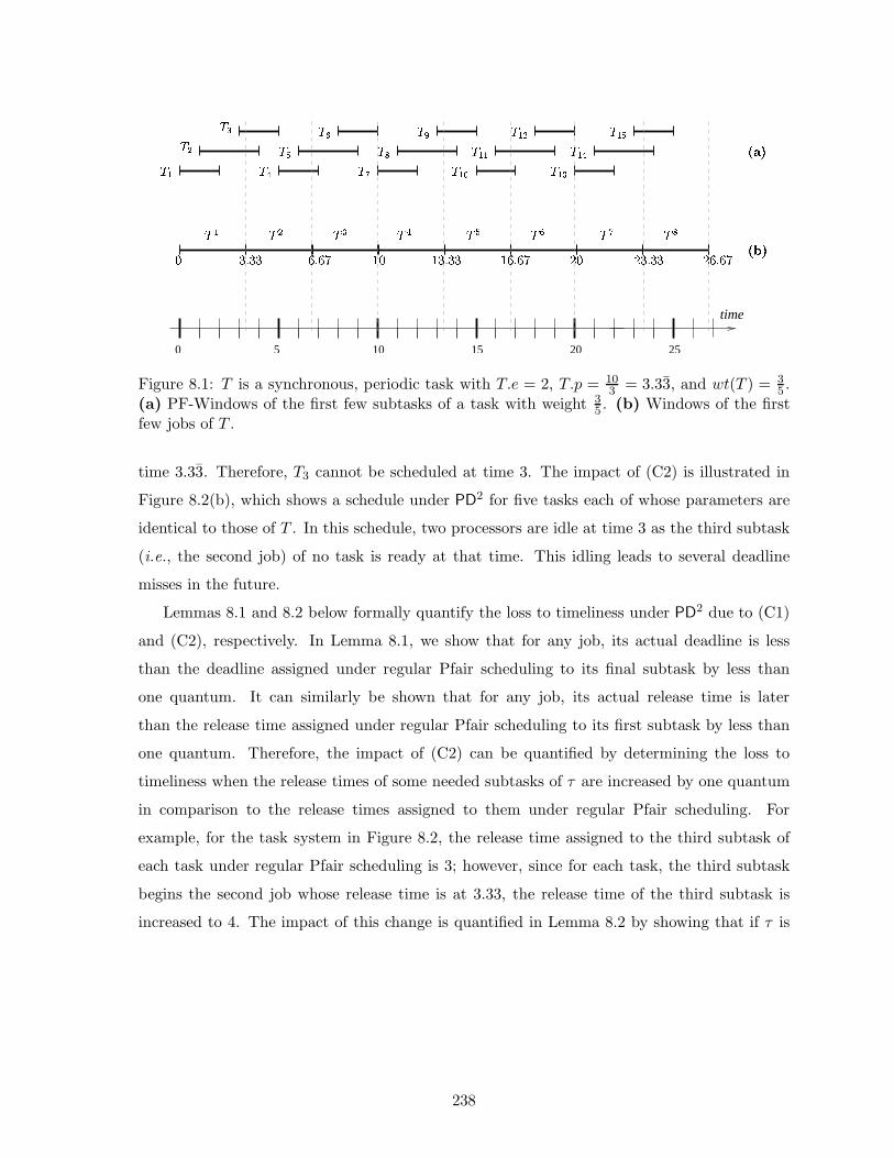
0 5 1510 20 25

time

�� ¡ �¢ �£ ¤¥¦

¤§¦��

��

�¡�¢�£

��©��

��

��

ª «¬«« ¬® ª «¬«« ¬® °ª °«¬«« °¬®

Figure 8.1: T is a synchronous, periodic task with T.e = 2, T.p = 103 = 3.33, and wt(T ) = 3

5 .(a) PF-Windows of the first few subtasks of a task with weight 3

5 . (b) Windows of the firstfew jobs of T .

time 3.33. Therefore, T3 cannot be scheduled at time 3. The impact of (C2) is illustrated in

Figure 8.2(b), which shows a schedule under PD2 for five tasks each of whose parameters are

identical to those of T . In this schedule, two processors are idle at time 3 as the third subtask

(i.e., the second job) of no task is ready at that time. This idling leads to several deadline

misses in the future.

Lemmas 8.1 and 8.2 below formally quantify the loss to timeliness under PD2 due to (C1)

and (C2), respectively. In Lemma 8.1, we show that for any job, its actual deadline is less

than the deadline assigned under regular Pfair scheduling to its final subtask by less than

one quantum. It can similarly be shown that for any job, its actual release time is later

than the release time assigned under regular Pfair scheduling to its first subtask by less than

one quantum. Therefore, the impact of (C2) can be quantified by determining the loss to

timeliness when the release times of some needed subtasks of τ are increased by one quantum

in comparison to the release times assigned to them under regular Pfair scheduling. For

example, for the task system in Figure 8.2, the release time assigned to the third subtask of

each task under regular Pfair scheduling is 3; however, since for each task, the third subtask

begins the second job whose release time is at 3.33, the release time of the third subtask is

increased to 4. The impact of this change is quantified in Lemma 8.2 by showing that if τ is

238

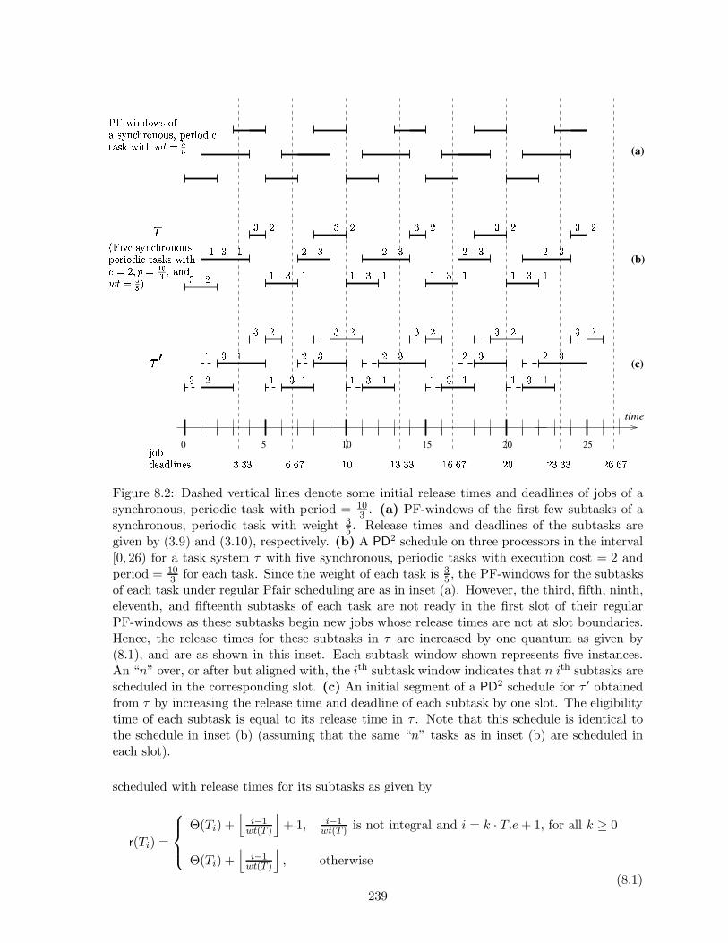
(a)

(b)

(c)

time

50 10 15 20 25

±²³ µ¶· ´ ¹²º »¼·½ ¾½µ¿±²ÀÁ½¿¶ÂÃÄÅÆÇÈÉÁ½ ¾ Á² Ê

Ë Ì ËÍÌ

ÎÈ½Ï¼ ²³ µ¶· ´ ¹²º»¼·½ ¾½µ ¿±²À²Á½¿¶ÐÄÍÑÒÄÓÔÅ Ñ ± ¾ÂÃÄÅÆÕ

Í

Ë Ì ËÍ Ì

Ì Í

Ë Ì ËÍ Ì

Ì Í

Ë Ì ËÍ Ì

Ì Í

Ë Ì ËÍ Ì

Ì ÍÖ Ì

× Ø¾¼±¾Ù½ ¼² ÌÚÌÌ ÛÚÛÜ ËÝ ËÌÚÌÌ ËÛÚÛÜ ÍÝ ÍÌÚÌÌ ÍÛÚÛÜ

Ì ÍË Ì Ë

Ì Í

Ì ÍÍ Ì

Ë Ì Ë Ë Ì ËÍ Ì

Ì Í

Ë Ì ËÍ Ì

Ì Í

Ë Ì ËÍ Ì

Ì ÍÖÞ

Figure 8.2: Dashed vertical lines denote some initial release times and deadlines of jobs of asynchronous, periodic task with period = 10

3 . (a) PF-windows of the first few subtasks of asynchronous, periodic task with weight 3

5 . Release times and deadlines of the subtasks aregiven by (3.9) and (3.10), respectively. (b) A PD2 schedule on three processors in the interval[0, 26) for a task system τ with five synchronous, periodic tasks with execution cost = 2 andperiod = 10

3 for each task. Since the weight of each task is 35 , the PF-windows for the subtasks

of each task under regular Pfair scheduling are as in inset (a). However, the third, fifth, ninth,eleventh, and fifteenth subtasks of each task are not ready in the first slot of their regularPF-windows as these subtasks begin new jobs whose release times are not at slot boundaries.Hence, the release times for these subtasks in τ are increased by one quantum as given by(8.1), and are as shown in this inset. Each subtask window shown represents five instances.An “n” over, or after but aligned with, the ith subtask window indicates that n ith subtasks arescheduled in the corresponding slot. (c) An initial segment of a PD2 schedule for τ ′ obtainedfrom τ by increasing the release time and deadline of each subtask by one slot. The eligibilitytime of each subtask is equal to its release time in τ . Note that this schedule is identical tothe schedule in inset (b) (assuming that the same “n” tasks as in inset (b) are scheduled ineach slot).

scheduled with release times for its subtasks as given by

r(Ti) =

Θ(Ti) +⌊

i−1wt(T )

⌋

+ 1, i−1wt(T ) is not integral and i = k · T.e + 1, for all k ≥ 0

Θ(Ti) +⌊

i−1wt(T )

⌋

, otherwise

(8.1)

239

then tardiness for the subtasks (not jobs) of τ is at most one quantum. Finally, Lemmas 8.1

and 8.2 are used to show that deadlines are missed by less than two quanta under PD2 if the

restriction that periods be integral is relaxed. For clarity and ease of description, we assume

that Θ(Ti) is integral. It can be shown that eliminating this assumption does not lead to any

additional loss to timeliness.

Lemma 8.1 Let τ be a sporadic task system such that the execution cost of every task in

τ is integral. Let T be a task in τ with a non-integral period. Then, for any job T k of T ,

d(T k) > d(Tk·T.e) − 1, where d(Ti) is as given by (3.10).

Proof: Since T k is the kth job of T , its deadline is given by

d(T k) = Θ(T k) + k · T.p, (8.2)

where, as discussed in the beginning of this section, Θ(T k) is the offset of T k.

As discussed in the beginning of this section again, subtasks T(k−1)·T.e+1, . . . , Tk·T.e comprise

the kth job of T , and since T is sporadic, each subtask of T k has the same offset, which is

equal to Θ(T k). Specifically, Θ(Tk·T.e) = Θ(T k). Therefore, by (3.10), we have

d(Tk·T.e) = Θ(T k) +

⌈

k · T.e

wt(T )

⌉

= Θ(T k) + dk · T.pe . (8.3)

By (8.2) and (8.3), d(Tk·T.e) − d(T k) < 1, from which the lemma follows. �

The next lemma makes use of two task systems that differ only in the release times and

deadlines assigned to their subtasks. Hence, in order to identify the task system under consid-

eration, we overload the release time and deadline functions to take a task system as a second

parameter. For instance, d(Ti, τ) will denote the deadline assigned to a subtask Ti in task

system τ .

Lemma 8.2 Let τ be a sporadic task system with an integral execution cost for every task

and a non-integral period for one or more tasks, and let Usum(τ) ≤ M . Let the deadline and

release time of every subtask Ti of every task T in τ (denoted d(Ti, τ) and r(Ti, τ)) be given

by (3.10) and (8.1), respectively. Let the b-bit and the group deadline be as given by (3.6) and

(3.7), respectively. Then, tardiness for subtasks of τ is at most one quantum under PD2, and

is worsened by at most one quantum under EPDF, in comparison to the tardiness to which τ

may be subject when all task periods are integral but no task weight is altered.

240

Proof: Let τ ′ be a task system obtained from τ such that τ ′ contains every subtask that is in

τ . Let r(Ti, τ′) and d(Ti, τ

′), the release time and deadline of subtask Ti in τ ′, be increased by

one quantum (in comparison to the values given by (3.9) and (3.10)) to Θ(Ti) +⌊

i−1wt(T )

⌋

+ 1

and Θ(Ti) +⌈

iwt(T )

⌉

+ 1, respectively. (Note that since r(Ti, τ) is given by (8.1) and not (3.9),

some subtasks can have equal release times in τ and τ ′.) Let the eligibility time of Ti in τ ′,

e(Ti, τ′), be the same as in τ . Hence,

e(Ti, τ′) = e(Ti, τ) ≤ r(Ti, τ).

For instance, if τ is an in Figure 8.2(b), then in τ ′, the subtasks that correspond to the first

few subtasks of τ are as in Figure 8.2(c). Since in τ ′, all release times and deadlines are

uniformly increased by one quantum (in comparison to those assigned under regular Pfair

scheduling), and the b-bit and group deadline are not altered for any subtask, the relative

priority between any two subtasks is unaltered under PD2 or EPDF by the increase in release

times and deadlines. Hence, since PD2 is optimal even when subtasks may be early released, it

is easy to see that every subtask Ti of τ ′ completes executing by d(Ti, τ′) when τ ′ is scheduled

under PD2. Similarly, a tardiness bound of q can be guaranteed to τ ′ under EPDF, where q

denotes the tardiness bound derived in Chapter 7 for a task system with the same maximum

task weight as that of τ ′.

By the definition of e(Ti, τ′), the IS-window of every subtask in τ ′ begins at the same

time as in τ , but is extended by one slot to the right (because d(Ti, τ′) = d(Ti, τ) + 1 holds

for every Ti). Thus, the relative priority between any two subtasks is the same in τ and τ ′.

Hence, since a subtask remains eligible from its eligibility time until it is scheduled, and the

relative priority between any two subtasks is the same in τ and τ ′, assuming a consistent

scheduler that resolves ties identically, the same set of subtasks contend for execution at each

slot in corresponding schedules for τ and τ ′. Also, the same set of subtasks is scheduled in

each slot. Hence, completion times are identical for every subtask in corresponding schedules

under the same algorithm (either PD2 or EPDF) for τ and τ ′. For example, initial segments

of schedules for τ and τ ′ under PD2 depicted in insets (b) and (c) of Figure 8.2 are identical.

Finally, as described above, since every subtask Ti of τ ′ meets its deadline under PD2, and

d(Ti, τ′) = d(Ti) + 1 = d(Ti, τ) + 1 for every Ti, tardiness for τ under PD2 is at most one

quantum. Similarly, tardiness for τ under EPDF is at most q + 1 quanta. �

The theorem below follows from Lemmas 8.1 and 8.2.

241

Theorem 8.1 Let τ be a sporadic task system with an integral execution cost for every task

and a non-integral period for one or more tasks, and let Usum(τ) ≤ M . Then, τ can be

scheduled under PD2 such that the tardiness of every job of τ is less than two quanta, and

under EPDF such that the tardiness of every job of τ is worsened by less than two quanta in

comparison to the tardiness to which the job may be subject if all task periods are integral, but

no task weight is altered.

Proof: One way of scheduling τ using Pfair scheduling algorithms is by assigning each subtask

Ti of τ a release time that is at least the release time of the job of which Ti is a part, and

appropriate values for its deadline and the two tie-break parameters. We propose the following

assignments: d(Ti), b(Ti), and D(Ti) are as given by (3.10), (3.6), and (3.7), respectively, and

r(Ti) is as defined in (8.1). As discussed earlier, release times assigned by (8.1) differ from

those assigned under regular Pfair scheduling by one quantum for certain subtasks. Refer to

Figure 8.2 for an example.

The release time of the kth job of T , T k, is given by r(T k) = Θ(T k)+(k−1) ·T.p. Subtasks

T(k−1)·T.e+1, . . . , Tk·T.e comprise the kth job of T , and it can be verified that the release time

assigned to the first subtask of T k using (8.1) is at or after r(T k). For example, in Figure 8.2(b),

the release time of the third job of each task is at time 6.67. The fifth subtask is the first

subtask of the third job and the release time assigned to it is 7. If subtasks of τ are assigned

values for the various parameters as proposed above, then by Lemma 8.2, tardiness for the

subtasks of τ is at most one quantum under PD2, and is worsened by at most one quantum

under EPDF in comparison to the tardiness bound that can be guaranteed if every task period

is integral. By Lemma 8.1, the deadline assigned to the last subtask of a job is less than one

quantum later than the actual deadline of the job. The theorem therefore follows. �

Tightness of the tardiness bound under PD2. In the schedule in Figure 8.2, the fourth

subtask of one of the five tasks does not complete executing until time 8. Since the execution

cost of each task is 2.0, it follows that the second job of one of the tasks does not complete

executing until that time, whereas its deadline is at time 6.66. Thus, tardiness for that job

is slightly more than 1.33 time units. It is easy to construct examples in which tardiness is

arbitrarily close to, but less than, two quanta under PD2. For example, consider a synchronous,

periodic task system τ with k · e+1 tasks with an execution cost of e and a period of e+ 1k for

each task, where k and e are positive integers. The weight of each task in τ is k·ek·e+1 and the

total utilization of τ is k · e. The deadline of the second job of each task is at 2 · e+ 2k , and it is

242

easy to show that the second job (i.e., subtask 2 · e) of e tasks do not complete executing until

time 2 · e + 2 for a tardiness of 2 − 2k . This tardiness can be made arbitrarily close to two by

choosing a large enough value for k, and therefore, the tardiness bound given by Theorem 8.1

is tight for PD2.

8.2 Scheduling with Non-Integral Execution Costs

Unfortunately, unlike in the case of task periods, we have not been able to identify an elegant

way of eliminating the restriction of Pfair scheduling that task execution costs be integral.

However, such tasks can be scheduled in a “Pfair-like” manner by using g-NP-EDF.

To see this, observe that one way of scheduling tasks with non-integral execution costs

is by dividing each job of a task into uniform-sized “sub-jobs,” allowing different sub-job

sizes, if needed, for different tasks, associating a pseudo-release and a pseudo-deadline with

each sub-job based on the parameters of its task, and scheduling sub-jobs non-preemptively

in an earliest-pseudo-deadline-first basis. There is to be no restriction on job migration in

that different sub-jobs of a job can execute on different processors. Since this algorithm is

essentially g-NP-EDF applied to sub-jobs, we will refer to it as EDF-sliced, and since g-NP-EDF

is not optimal, EDF-sliced is not optimal, either. A tardiness bound that can be guaranteed to

a task system τ under EDF-sliced can be computed using the formula provided in Chapter 4 (in

Corollary 4.3) by using the highest M−1 task utilizations for µ1, . . . , µM−1, and highest M sub-

job execution costs of tasks (as opposed to the highest M task execution costs) for ε1, . . . , εM .

Since the tardiness bound of g-NP-EDF given by Corollary 4.3 increases with increasing values

for εi, tardiness can be lowered by choosing smaller sub-job sizes at the expense of increased

scheduling and migration overhead.

Though straightforward to compute, for completeness, we provide formulas for the pseudo-

release and pseudo-deadline of the ith sub-job of a task (assuming that sub-jobs are numbered

sequentially from the first job). At the risk of some notational overload, let Ti denote the ith

sub-job of T . Let T.s denote the number of sub-jobs into which each job of T is sliced. Then

the pseudo-release r(Ti) and the pseudo-deadline d(Ti) of Ti are as follows. (In the formulas

below, Θ(Ti) is the offset of the ith sub-job, and if T is sporadic, then all the sub-jobs of a job

have the same offset.)

r(Ti) = Θ(Ti) +(i − 1) · T.e

T.s · wt(T )= Θ(Ti) +

(i − 1) · T.p

T.s

243

d(Ti) = Θ(Ti) +i · T.e

T.s · wt(T )= Θ(Ti) +

i · T.p

T.s

For an example application of the above formulas, let T be a synchronous, periodic task with

T.e = 3.2 and T.p = 5, and let each job of T be subdivided into two sub-jobs (i.e., T.s = 2).

Then, T.pT.s = 2.5, and r(Ti) = 2.5× (i−1) and d(Ti) = 2.5× i (since T is synchronous, periodic,

Θ(Ti) = 0). The first sub-job of the first job, T1, has a deadline of 2.5 and the second sub-job

of the same job has a release time of 2.5.

Implementation considerations. Handling non-integral values for sub-job deadlines is

similar to handling non-integral periods under g-NP-EDF, which is described in the next section.

However, handling non-integral execution costs for sub-jobs cannot be considered to be similar

to handling non-integral execution costs for jobs. This is due to the following facts. Assuming a

well-behaved system in which tasks do not overrun, job completions need not be policed by the

scheduler, and the process thread corresponding to each job either terminates or relinquishes

voluntarily when it has executed for its WCET or earlier. In other words, the event that marks

the completion of a job is part of the job, upon whose occurrence the scheduler is invoked.

On the other hand, sub-jobs are in some sense “artificial,” and the execution cost of a sub-job

can be viewed as simply defining a point within the job’s execution at which its deadline is

altered. Further, there is no indication in the job itself that marks the completion of a sub-job,

and hence, sub-job completions need to be monitored and enforced using timers. Therefore,

practical considerations may require that all sub-jobs except the last of any job have execution

costs that are integral multiples of the minimum possible system timer period. This timer

period may be equal to the system quantum size in tick-based implementations. (Tick-based

scheduling is discussed in detail in Chapter 9.) To account for such varying sub-job execution

costs, sub-job release times and deadlines given earlier also need to be appropriately modified.

As before, letting T.s denote the number of sub-jobs per job of T , the first T.s−1 sub-jobs can

be assigned an execution cost of⌈

T.eT.s

⌉

(provided⌈

T.eT.s

⌉

· (T.s− 1) < T.e) or⌊

T.eT.s

⌋

each, and the

remaining execution cost can be assigned to the final sub-job. Let T.e1 denote the execution

cost of each of the initial T.s − 1 sub-jobs of a job of T and T.e2 that of the final sub-job.

Then, T.e2 = T.e− (T.s−1) ·T.e1, and the release time and deadline of the ith sub-job, Ti, can

be computed as follows. Note that because there are T.s sub-jobs per job of T , Ti is part of

job⌈

iT.s

⌉

. Let I denote the sub-job index of Ti within its job, i.e., I = ((i − 1) mod T.s) + 1.

244

Then,

r(Ti) = Θ(Ti) +

(⌈

i

T.s

⌉

− 1

)

· T.p +(I − 1) · T.e1

wt(T )

d(Ti) =

Θ(Ti) + i·T.pT.s , if T.s | i

Θ(Ti) + (⌈

iT.s

⌉

− 1) · T.p + I·T.e1wt(T ) , otherwise.

For the example task considered earlier (with uniform-sized sub-jobs), letting T.s = 3, T.e1 =⌊

T.eT.s

⌋

=⌊

3.23

⌋

= 1, T.e2 = 3.2 − (T.s − 1) · T.e1 = 1.2. Since T is synchronous, periodic, all

offsets are zero. Hence, r(T1) = 0, d(T1) = r(T2) = 1×13.2/5 = 1.5625, d(T2) = 2×1

3.2/5 = 3.125,

r(T3) = 3.125, and d(T3) = 5. As discussed in Section 4.4, sub-jobs with varying execution

costs can be modeled using the extended sporadic task model described there, and the tardiness

bounds derived in Chapter 4 for g-NP-EDF apply.

8.3 Non-Integral Periods under EDF-based Algorithms

Throughout this dissertation, we have assumed that periods and execution costs can be non-

integral for non-Pfair algorithms. While a non-integral execution cost is not likely to be

problematic in practical implementations, a non-integral period may not be acceptable in tick-

based implementations. As mentioned earlier, tick-based scheduling is discussed in detail in

Chapter 9, and, under it, new job releases are noticed only at quantum boundaries. Hence,

if the period of a task is non-integral, then its jobs may arrive in the middle of a quantum,

but will not be considered for scheduling until the next quantum boundary. This is similar to

the problem faced under Pfair scheduling when periods are non-integral, which was discussed

in Section 8.1. The transformation technique that was used in Lemma 8.2 can be used to

show that if practical considerations require periods to be integral, but one or more tasks have

non-integral periods, then tardiness under g-EDF, g-NP-EDF, and EDF-sliced is worsened by

at most one quantum. (The same technique can be used because the tardiness bounds derived

for g-EDF and g-NP-EDF in Chapter 4 apply even if jobs may be early released.) Furthermore,

by the same argument, if a task system τ is schedulable without deadline misses under one of

these algorithms even if jobs may be early released, then deadlines will be missed by at most

one quantum if tasks in τ have non-integral periods but scheduling is tick-based.

Finally, though the tardiness bounds derived for EDF-fm in Chapter 5 cannot be shown to

hold if jobs of migrating tasks are arbitrarily early-released, the bounds can be shown to hold

245

if each job is early released by at most one quantum. Hence, the transformation technique

of Lemma 8.2 can be used to show that tardiness for fixed tasks is worsened by at most one

quantum and that migrating tasks may miss their deadlines by at most one quantum.

8.4 Summary

In this chapter, we considered the Pfair scheduling of tasks with non-integral periods and

execution costs. We showed that a task system with non-integral periods for one or more

tasks but integral execution costs for all the tasks can be scheduled under PD2 such that job

deadlines are missed by less than two quanta, and under EPDF such that the tardiness bounds

guaranteed to its jobs is worsened by less than two quanta in comparison to what can be

guaranteed to a task system with comparable task weights but integral task periods. We also

proposed an algorithm called EDF-sliced for scheduling tasks in a “Pfair-like” manner when

both task periods and execution costs may be non-integral. Finally, we considered the impact

to timeliness of non-integral periods in tick-based implementations of non-Pfair scheduling

algorithms.

246

Chapter 9

Performance Evaluation of Scheduling

Algorithms

In the previous chapters, we analytically determined some soft real-time guarantees that can be

provided by some multiprocessor real-time scheduling algorithms. In this chapter, we attempt

to compare the practical performance of the algorithms through simulations. Our metrics

for comparison are the percentage of task systems for which each algorithm can guarantee

bounded tardiness and the average tardiness bound guaranteed after accounting for system

implementation overheads.

The tardiness bound guaranteed by each algorithm considered in this dissertation for a

task system is dependent upon the total system utilization, Usum, and holds only if Usum is

at most the number of processors. Usum in turn depends on the WCETs and periods of the

tasks in τ . As discussed in Chapter 1, system implementation overheads, such as scheduler

invocations, and task preemption and migration costs, can take time away from the application

tasks at hand and delay them. It was also mentioned that one way of accounting for the time

lost due to overheads is to inflate, in an efficient (i.e., non-pessimistic) and a safe manner,

the WCETs of tasks above the time required for the execution of each task on a dedicated

processor (i.e., in isolation). Further, the extent of the overhead from each extrinsic source can

vary with the scheduling algorithm, characteristics of the application, and the implementation

platform. Thus, in practice, the tardiness bound guaranteed by an algorithm is dependent on

the overheads incurred (because it is dependent on Usum), apart from the intrinsic properties

of the algorithm.

Therefore, in this chapter, we seek to empirically determine how the different algorithms

compare if external overheads are accounted for. We also include the partitioned-EDF (p-

EDF) algorithm in our study. Recall that p-EDF is a no-migration algorithm with EDF as the

per-processor scheduler, and as such does not incur any migration overhead. Further, a task

system’s tardiness under p-EDF is zero if it can be partitioned among the available processors,

and unbounded otherwise. Since partitioning algorithms are currently preferred to global

algorithms for scheduling real-time multiprocessor systems, we evaluate the other algorithms

with respect to p-EDF, which is believed to be among the best partitioning algorithms.

The rest of this chapter is organized as follows. Our assumptions regarding scheduler

implementations and task models are stated in Section 9.1. This is followed by a discussion

of some significant external sources of overhead in Section 9.2. Then, in Section 9.3, for each

algorithm, we give formulas for determining the WCET of a task in the presence of overheads.

Finally, a simulation-based evaluation of the algorithms is presented in Section 9.4.

9.1 Assumptions

Before discussing system overheads, we state some notational conventions and our assumptions

concerning how tasks are specified and scheduled. As mentioned in Chapter 1, we assume that

the underlying hardware platform is a symmetric, shared-memory multiprocessor.

The WCET of a task T on a dedicated processor will be referred to as its base WCET and

will be denoted T.e(b). The WCET obtained after accounting for overheads will be referred to

as its inflated WCET, or simply WCET, when unambiguous from context. T.e will refer to T ’s

inflated WCET.

Assumption A1: All task periods are assumed to be expressed as integral multiples of the

system’s quantum size. However, the base WCET of each task may be non-integral (but a

positive, rational number). As shown in Chapter 8, if periods are non-integral, then under

all the algorithms considered, tardiness is worsened by comparable amounts that are minimal.

Hence, assuming non-integral values for periods does not lead to a loss of generality. Recall

that Pfair algorithms require integral values for execution costs as well. This requirement is

met by simply rounding up each non-integral inflated WCET. Thus, a non-integral execution

cost results in an extra source of overhead for a Pfair algorithm.

Assumption A2: Scheduling is time driven (also referred to as tick scheduling) under the

EPDF and PD2 Pfair algorithms. As discussed in Chapter 3, quanta are assumed to be aligned

248

on all processors, and scheduling decisions are made only at the beginning of each quantum

on each processor. If a Pfair subtask completes executing in the middle of a quantum, then

the remainder of that quantum on the associated processor is wasted.

Scheduling under the remaining algorithms is a mix of time-driven and event-driven schedul-

ing . As with Pfair algorithms, each processor’s scheduler is invoked at the beginning of each

quantum to context switch to a higher-priority ready job, if any, and in that sense is time

driven. However, unlike Pfair algorithms, a processor’s scheduler is also invoked whenever a

job completes executing on that processor, even if the completion time is within a quantum

(i.e., not at a quantum boundary). In this sense, scheduling is event driven. For illustration,

refer to Figure 9.2(a) (considered in detail later), which shows an example schedule under g-

NP-EDF. In this schedule, the first jobs of U and V complete execution at time 3.5. Hence, the

scheduler is invoked at time 3.5, even though this time is not a quantum boundary, to schedule

at most two ready, but waiting, jobs with the highest priorities. As with Pfair algorithms, we

assume that quanta are aligned on all processors. Relaxing this assumption will worsen the

tardiness bounds guaranteed by the amount by which the quanta are misaligned.

Since periods are assumed to be integral multiples of the quantum size, in a periodic

task system, a job becomes ready at a quantum boundary only. Hence, in periodic systems,

tardiness is not impacted due to time-driven scheduling. On the other hand, in a sporadic task

system, a higher-priority job may arrive within a quantum. In such systems, not scheduling a

higher-priority job as soon as it arrives worsens the tardiness of a job by at most one quantum

under all of the algorithms, and is thus negligible. Hence, like Assumption A1, this assumption

also does not lead to a loss of generality.

It should also be noted that, unlike Pfair algorithms, tick scheduling is not mandatory for

non-Pfair algorithms. In implementations that are entirely event driven, the overhead due to

tick scheduling is eliminated; the remaining overheads should be similar to those incurred in

implementations based on tick scheduling.

Tick scheduling is generally implemented by delivering timer interrupts to each processor

at a frequency of nQ interrupts/sec. (or, equivalently, by using a tick period of Q

n ), where

Q is the quantum size and n is a positive integer. n ticks then comprise a quantum, and a

new quantum can be thought of as starting at the beginning of tick k · n, for all k ≥ 0. The

scheduler on each processor is invoked at the beginning of each new quantum.

249

Assumption A3. The amount of data output by a job that is also used by a later job of

the same task is minimal. This assumption implies that when a job is scheduled and begins

execution for the first time, its working set is not resident on a remote cache in a read-write

state. Hence, a new job does not incur overhead involved in invalidating remote cache lines.

We believe this to be a reasonable assumption for applications that use time-varying data

such as tracking systems. Relaxing this assumption in a non-pessimistic manner requires

application-specific details.

Assumption A4. The time taken to load each job’s initial working set is included in its

base WCET. Because A3 is assumed, this assumption does not cause the base WCET to be

dependent on the algorithm.

(Assumptions A3 and A4 will be clearer when preemption and migration overheads are con-

sidered.)

Assumption A5. Jobs (or subtasks) are not early released.

9.2 System Overheads

In this section, we discuss several external sources of overhead and the impact of each on

the various algorithms. These overheads include scheduler , context-switching , cache-related

preemption, and migration costs.

Each time a job is preempted, scheduling and context-switching overheads are incurred,

and migration overhead is incurred if the preempted job is later scheduled on a different pro-

cessor. While a job preemption is necessary for a migration, scheduling and context-switching

overheads can be incurred even without a preemption, such as, when a lower-priority job is

scheduled after a higher-priority job completes execution. Hence, by cache-related preemption

overhead, we refer to the overhead due to the eviction from cache of a job’s working set, which

will be needed later when the job resumes execution on the same processor. This overhead

includes neither the scheduling and context-switching costs nor the overhead due to migration.

Before delving into a detailed discussion of the above overheads, we will briefly describe

relevant scheduler data structures.

250

Scheduler data structures. One common approach for implementing periodic tasks is by

associating a release queue with each needed future quantum. A quantum’s release queue is

a priority queue of all the jobs (or subtasks) that are to be released at the beginning of that

quantum. Whenever a job (or subtask) completes executing, if the release time of the next job

(or subtask) of the same task is later than the current time, then the next job (or subtask) is

enqueued onto the release queue associated with its release time; otherwise, it is enqueued onto

the ready queue. Each release queue is merged with the ready queue1 at the queue’s release

time. Hence, the number of release queues to be maintained at a given time is bounded by

the number of tasks. Further, the release time of any non-empty queue is at most pmax quanta

in the future, where pmax denotes the maximum period of any task. (Each queue is local to a

processor under partitioning and is globally shared otherwise.)

In sporadic systems, job releases are assumed to be triggered by interrupts, either hardware

or software, and a job may arrive within a quantum. (Job releases dependent on events external

to the system will be delivered using hardware interrupts, whereas those dependent on events

in other tasks can be signaled using software interrupts, such as POSIX signals.) Each arriving

job is queued in the pending queue, which is a queue of all jobs arriving within the current

quantum (as opposed to a release queue). The pending queue is merged with the ready queue

at the beginning of the next quantum. Therefore, there is one logical pending queue under

global scheduling, and one pending queue per processor under partitioning (as opposed to

multiple release queues).

Under both Pfair and non-Pfair algorithms, the scheduler is invoked at the beginning of

each quantum. However, under the non-Pfair algorithms considered here, a change in the set

of executing jobs (i.e., jobs that are scheduled on the various processors) may be needed only

if some current job completes execution, or some new job (that was not ready at the previous

quantum) becomes ready, i.e., the release queue of the next quantum (or pending queue) is

non-empty, and the job at the head of the release (or pending) queue has a higher priority than

some executing job. Even if no change is needed to the set of executing jobs, housekeeping

functions, such as, merging a release (or pending) queue with the ready queue, should be

performed at the beginning of each quantum to ensure that the scheduler data structures are

updated and consistent. We refer to the time taken at each quantum boundary to perform

such housekeeping functions, including the time taken to ensure that no change is needed to

1A ready queue is a priority queue of ready jobs (or subtasks).

251

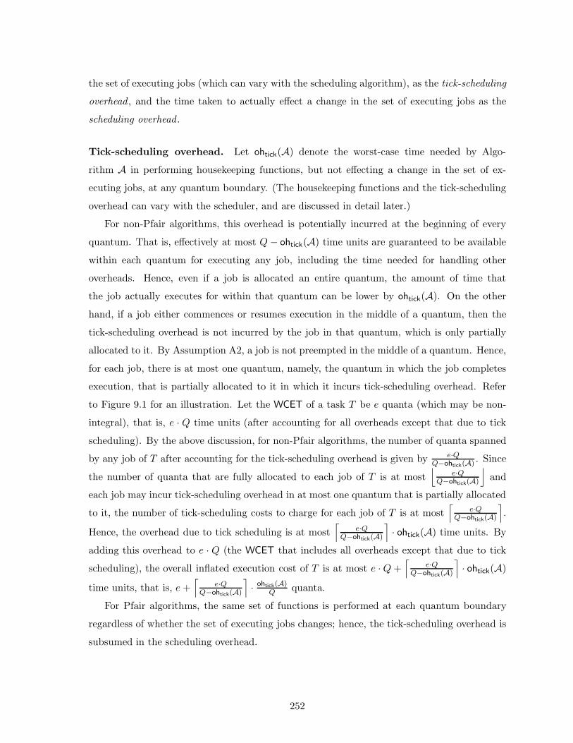
the set of executing jobs (which can vary with the scheduling algorithm), as the tick-scheduling

overhead , and the time taken to actually effect a change in the set of executing jobs as the

scheduling overhead .

Tick-scheduling overhead. Let ohtick(A) denote the worst-case time needed by Algo-

rithm A in performing housekeeping functions, but not effecting a change in the set of ex-

ecuting jobs, at any quantum boundary. (The housekeeping functions and the tick-scheduling

overhead can vary with the scheduler, and are discussed in detail later.)

For non-Pfair algorithms, this overhead is potentially incurred at the beginning of every

quantum. That is, effectively at most Q − ohtick(A) time units are guaranteed to be available

within each quantum for executing any job, including the time needed for handling other

overheads. Hence, even if a job is allocated an entire quantum, the amount of time that

the job actually executes for within that quantum can be lower by ohtick(A). On the other

hand, if a job either commences or resumes execution in the middle of a quantum, then the

tick-scheduling overhead is not incurred by the job in that quantum, which is only partially

allocated to it. By Assumption A2, a job is not preempted in the middle of a quantum. Hence,

for each job, there is at most one quantum, namely, the quantum in which the job completes

execution, that is partially allocated to it in which it incurs tick-scheduling overhead. Refer

to Figure 9.1 for an illustration. Let the WCET of a task T be e quanta (which may be non-

integral), that is, e · Q time units (after accounting for all overheads except that due to tick

scheduling). By the above discussion, for non-Pfair algorithms, the number of quanta spanned

by any job of T after accounting for the tick-scheduling overhead is given by e·QQ−ohtick(A) . Since

the number of quanta that are fully allocated to each job of T is at most⌊

e·QQ−ohtick(A)

⌋

and

each job may incur tick-scheduling overhead in at most one quantum that is partially allocated

to it, the number of tick-scheduling costs to charge for each job of T is at most⌈

e·QQ−ohtick(A)

⌉

.

Hence, the overhead due to tick scheduling is at most⌈

e·QQ−ohtick(A)

⌉

· ohtick(A) time units. By

adding this overhead to e · Q (the WCET that includes all overheads except that due to tick

scheduling), the overall inflated execution cost of T is at most e · Q +⌈

e·QQ−ohtick(A)

⌉

· ohtick(A)

time units, that is, e +⌈

e·QQ−ohtick(A)

⌉

· ohtick(A)Q quanta.

For Pfair algorithms, the same set of functions is performed at each quantum boundary

regardless of whether the set of executing jobs changes; hence, the tick-scheduling overhead is

subsumed in the scheduling overhead.

252

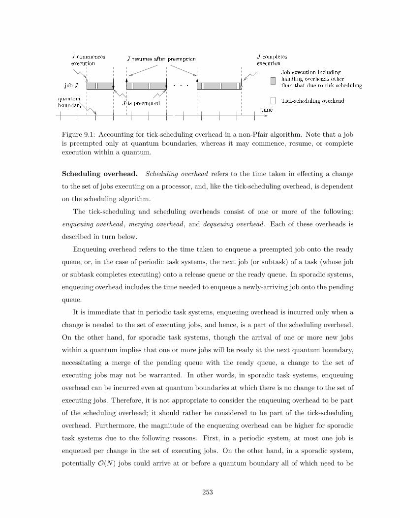
ß ß ß

à áâããäåáäæäçäáèéêâå à ëäæèãäæ ìíéäë îëääãîéêâå à áâãîïäéäæäçäáèéêâåðâñäçäáèéêâåêåáïèòêåóôìåòïêåóâõäëôäìòæ âéôäëéôìåéôìé òèä éâéêáöæáôäòèïêåó÷êáöøæáôäòèïêåóâõäëôäìòéêãäà êæ îëääãîéäòùèìåéèãñâèåòìëú

ûâñà

Figure 9.1: Accounting for tick-scheduling overhead in a non-Pfair algorithm. Note that a jobis preempted only at quantum boundaries, whereas it may commence, resume, or completeexecution within a quantum.

Scheduling overhead. Scheduling overhead refers to the time taken in effecting a change

to the set of jobs executing on a processor, and, like the tick-scheduling overhead, is dependent

on the scheduling algorithm.

The tick-scheduling and scheduling overheads consist of one or more of the following:

enqueuing overhead , merging overhead , and dequeuing overhead . Each of these overheads is

described in turn below.

Enqueuing overhead refers to the time taken to enqueue a preempted job onto the ready

queue, or, in the case of periodic task systems, the next job (or subtask) of a task (whose job

or subtask completes executing) onto a release queue or the ready queue. In sporadic systems,

enqueuing overhead includes the time needed to enqueue a newly-arriving job onto the pending

queue.

It is immediate that in periodic task systems, enqueuing overhead is incurred only when a

change is needed to the set of executing jobs, and hence, is a part of the scheduling overhead.

On the other hand, for sporadic task systems, though the arrival of one or more new jobs

within a quantum implies that one or more jobs will be ready at the next quantum boundary,

necessitating a merge of the pending queue with the ready queue, a change to the set of

executing jobs may not be warranted. In other words, in sporadic task systems, enqueuing

overhead can be incurred even at quantum boundaries at which there is no change to the set of

executing jobs. Therefore, it is not appropriate to consider the enqueuing overhead to be part

of the scheduling overhead; it should rather be considered to be part of the tick-scheduling

overhead. Furthermore, the magnitude of the enqueuing overhead can be higher for sporadic

task systems due to the following reasons. First, in a periodic system, at most one job is

enqueued per change in the set of executing jobs. On the other hand, in a sporadic system,

potentially O(N) jobs could arrive at or before a quantum boundary all of which need to be

253

enqueued.2 Secondly, in a sporadic system, each job arrival can require the interrupt service

routine (ISR) or the signal handler of the job-arrival interrupt to be invoked, and hence,

enqueues are only logically but not physically part of the scheduler. On the other hand, in

a periodic system, the cost of invoking a separate ISR before an enqueue operation can be

eliminated because the single enqueue can be physically part of the scheduler.

Merging overhead refers to the time taken at a quantum boundary to merge the next

quantum’s release (pending) queue with the ready queue in periodic (sporadic) systems. As

discussed earlier (in the context of scheduler data structures), a merge operation may po-

tentially be required at each quantum boundary, and hence, is a part of the tick-scheduling

overhead.

Finally, dequeuing overhead refers to the time required to extract or dequeue the highest

priority job from the ready queue, and is a part of the scheduling overhead.

The time complexities of each of the above overheads, and hence, those of tick-scheduling

and scheduling, depend on the size of the ready queue (from which the highest priority job

is chosen) and the sizes of the release and pending queues and whether a processor’s queues

are exclusive to it or shared. Since each task can have at most one ready job (or subtask)

at any time (even though more than one is pending), for global algorithms, the size of the

global ready queue is at most N . Under p-EDF and EDF-fm, the number of tasks assigned to

a processor is N − (M − 1) in the worst-case (assuming at least one task is assigned to each

processor), and NM on an average. (It should be noted that in sporadic systems, additional

mechanisms are needed to ensure that multiple pending jobs of a task are not present in the

ready queue. Otherwise, the size of the ready queue will depend on the number of jobs that

can be pending per task, which in turn depends on the tardiness bound. One mechanism is to

associate a pending queue per task, as opposed to a single common pending queue for all the

tasks, and enqueue each arriving job onto the pending queue of its task in a FIFO manner. At

each quantum boundary, only jobs at the head of each pending queue, and whose predecessors

have completed execution, should be merged with the ready queue.) In a periodic system,

because a job is enqueued onto a release queue only after its predecessor completes executing,

each task can have at most one job in all the release queues taken together. Hence, the size of

2Recall that in a periodic system, a new job is enqueued (either in a release queue or in the ready queue)when the prior job of the same task completes. Hence, though O(N) jobs can have their release times at somequantum boundary, such as the hyperperiod, this does not imply that O(N) jobs are enqueued at that time.The number of jobs enqueued at any time, including the hyperperiod, is given by the number of jobs completingexecution at that time, which is at most M .

254

a release queue has the same upper bound as that of the ready queue. Similarly, in a sporadic

system, since at most one job per task will be merged with the ready queue at any quantum,

the size of the pending queue can be taken to be at most N in determining the time complexity

of a merge.

Digression: Implementation of EDF-fm. Before continuing with the discussion of time

complexity, a brief description of how EDF-fm can be implemented is in order. Recall that

under EDF-fm, each processor is assigned some number of fixed tasks and at most two migrating

tasks, and a fixed task is assigned to a single processor, while a migrating task is assigned to two

processors. Also recall that each job of a migrating task executes on one of its two processors

only. Further, the processor to which a migrating task’s job is assigned can be determined

based on the job index. Hence, if a migrating task is periodic, each of its processor schedulers

can easily determine the release time of the next job to be assigned to it, and can enqueue it

in the appropriate release queue when the current job of that task completes execution. (Such

an approach is sufficient since migrating tasks have zero tardiness.) On the other hand, if a

migrating task is sporadic, then each of its job arrivals can be programmed to trigger interrupts

on both of its processors. Here again, since the processor on which the job executes depends

on the job index, one of the processors can simply ignore arrival interrupts that are not meant

for it. Further, the two logical ready queues (one each for the ready jobs of fixed and migrating

tasks) associated with each processor can be implemented using a single physical ready queue

with a bit to denote whether a job belongs to a fixed task. Thus, implementing EDF-fm incurs

very little overhead, if any, in comparison to p-EDF.

Scheduler time complexity. We now turn to determining the worst-case time complexity

of the various priority-queue operations, and the total complexity of the sequence of operations

associated with scheduling and tick-scheduling. We will first ignore synchronization costs

incurred under global algorithms and include them later. Assuming that binomial heaps3 [117]

are used for implementing the ready queue and release queues, from our earlier discussion on

queue sizes, it follows that the worst-case cost of one enqueue, dequeue, or merge operation is

O(lg N) under all the algorithms for both periodic and sporadic systems. Hence, for periodic

systems, the worst-case complexity of both tick-scheduling and scheduling on any processor

3The worst-case time complexity of merging two binomial heaps is O(lg n) whereas it is O(n) for binary heaps,where n is the total number of elements in the two heaps. Further, binomial heaps are not more complicatedthan binary heaps to implement.

255

in O(lg N). On the other hand, for sporadic systems, while the worst-case complexity of

scheduling is O(N), that of tick-scheduling is O(N + lg N). This is because, O(N) jobs

(or subtasks) can arrive within a quantum, or be at the heads of the pending queues of

tasks, waiting to be merged. Constructing a binomial heap for the pending jobs that need

to be merged requires O(N) time, while merging the constructed heap with the ready queue

requires O(lg N) time. If tasks are partitioned approximately evenly among processors, then

the complexity of scheduling under p-EDF and EDF-fm can be lowered to O(lg NM ) for periodic

systems, and O( NM + lg N

M ) for sporadic systems.

We now consider the overhead incurred by global scheduling algorithms due to the use of

shared, global queues. Apart from having to deal with larger queue sizes, global algorithms

also suffer from the drawback that accesses to the shared queues must be serialized. Hence,

in the worst case, any processor waits for every other processor to complete its scheduling or

tick-scheduling operations. Thus, for both periodic and sporadic task systems, the complexity

of scheduling under global algorithms is O(M lg N). Since “merging” is the predominant

source of tick-scheduling overhead, and at most one processor needs to perform a merge for

any quantum, for periodic systems, the complexity of tick scheduling on each processor is

O(M + lg N) (and not O(M + M lg N)). The term M in O(M + lg N) accounts for the

constant-time overhead incurred on each processor to ensure that the merge has completed.

Similarly, for sporadic systems, the complexity of tick-scheduling overhead per processor is

O(M + N + lg N) (and not O(M + MN + M lg N)).

Context-switching overhead. Context-switching overhead refers to the actual cost of

switching between two tasks and does not include any task-specific cache-related overheads.

Overhead due to context switches primarily includes the time needed to save the hardware

context of the preempted or completing job in its process control block (PCB), load into cache

the PCB of the newly-scheduled job, and populate needed hardware registers from the loaded

PCB. If tasks do not share a common address space, then some additional overhead may be

incurred to invalidate and repopulate the translation look-aside buffer (TLB), and to load into

cache the page-table entries of the task that is being switched to. The cost of this overhead

should be nearly equal for all the algorithms.

Cache-related preemption overhead. This overhead refers to the delay associated with

servicing the cache misses suffered by a preempted job (misses that would have been hits but

256

for the preemption) when it resumes execution on the same processor (that it executed upon

before preemption). Preemption overhead4 is maximized when the tasks executing on all the

processors load their caches at the same time. Further, the delay depends on the amount of

data and instructions being fetched. Hence, the worst-case preemption cost is dependent on

task characteristics such as the size of its working set and its code size, and is independent of

the scheduling algorithm. Though it may be argued that this overhead can be incurred by a

newly-scheduled job also, and not just a job resuming execution after a preemption, we assume

that Assumption A4 holds.

Migration overhead. This overhead refers to the delay associated with servicing the cache

misses suffered by a preempted job when it resumes execution on a different processor. Even

though a preempted job is assumed in this case to resume execution on a different processor,

the worst-case migration cost is the same as the worst-case preemption cost if the data being

loaded is not resident on another processor’s cache (specifically, the processor on which the job

executed before the preemption) in a conflicting state (i.e., read-only versus read-write or read-

write versus read-write states). Otherwise, additional delay may be incurred in invalidating

appropriate cache lines in the cache of the first processor. (As with preemption overhead, the

worst case is when data is moved from a remote cache to the local cache on each processor,

though such a scenario seems highly unlikely.) Hence, since code segments are read-only,

migration costs are the same as preemption costs for instructions. (Note that an un-flushed

cache constitutes a worst-case scenario if a job migrates and a best-case scenario if the job

resumes on the same processor.) Finally, because jobs do not migrate under p-EDF, EDF-fm,

or NP-EDF, by Assumptions A3 and A4, migration overhead is zero for these three algorithms.

For the remaining algorithms, it is dependent on the working set size of the migrating task.

Hence, for a given task, the worst-case value should be identical for all unrestricted-migration

algorithms.

The worst-case overhead incurred by Algorithm A due to each of the above factors will be

denoted using the following notation. Since cache-related preemption and migration overheads

are dependent on task characteristics, these overheads take a task as a second parameter.

ohtick(A)def= overhead due to tick scheduling

4When unambiguous, we will refer to cache-related preemption overhead as just preemption overhead.

257

ohsch(A)def= scheduling overhead

ohcs(A)def= context-switching overhead

ohpr(A, T )def= preemption overhead

ohmig(A, T )def= migration overhead

9.3 Accounting for Overheads

In this section, we show how to account for the overheads discussed in Section 9.2, except the

overhead due to tick scheduling, under each algorithm considered. For non-Pfair algorithms,

the tick-scheduling overhead ohtick(A) should be incorporated using the formula provided in

Section 9.2 after the remaining overheads are accounted for as described below. We do discuss

elements that contribute to ohtick(A) (apart from the merging overhead discussed earlier) and

how to determine this value for each algorithm. For Pfair algorithms, as mentioned earlier, the

tick-scheduling overhead is included in the scheduling overhead. Our approach to accounting

for all the overheads considered is similar to that commonly used in work on real-time systems.

We will begin with g-NP-EDF.

Algorithm g-NP-EDF. Since there are no preemptions under g-NP-EDF, each job is sched-

uled exactly once. Thus, the total number of scheduling decisions (i.e., the total number of

dequeue operations in which the highest priority job is dequeued from the ready queue) needed

to effect changes in the set of executing jobs is equal to the total number of jobs. Similarly, the

total number of context switches is equal to the total number of jobs. Hence, overhead due to

scheduling and context switches is fully accounted for under g-NP-EDF if each job is charged

with one worst-case scheduling cost and one worst-case context-switching cost (to account for

scheduling that job and context switching to it). Refer to Figure 9.2 for an example. Inset (a)

shows an NP-EDF schedule in which overheads are assumed to be zero. If this assumption does

not hold, then job executions may be delayed due to scheduling and context switching costs

as shown in inset (b). Since there are no job preemptions or migrations, by Assumption A3,

cache-related preemption and migration costs are zero. Therefore, overhead under g-NP-EDF

(excluding that due to tick scheduling) can be fully accounted for if the WCET of each task

T is determined as follows. (Recall that T.e and T.e(b) denote T ’s inflated and base WCETs,

258

üýþÿ

��

��

��

��

��

��

� �� 0 1 2 3 4 5 6 7 0 1 2 3 4 5 6 7

�� !�"�#�� !�"�

$��%&'( %&'(

)*+,- .,/(012&3456(*/(70 8.56(*/(709:; 9<;)*+, =

Figure 9.2: Example g-NP-EDF schedules with (a) zero overhead and (b) non-zero overhead.

respectively.)

T.e = T.e(b) + ohsch(g-NP-EDF) + ohcs(g-NP-EDF)

Under g-NP-EDF, tick-scheduling overhead consists of the time taken at the beginning of a

quantum to merge that quantum’s release queue or the pending queue with the ready queue.

Although this overhead is incurred on at most one processor, since tasks are not bound to

processors, the worst case is to assume that the overhead is incurred on every processor, and

to charge each task.

Algorithm g-EDF. g-EDF differs from g-NP-EDF in that jobs may be preempted. Hence,

overhead under g-EDF is higher than that under g-NP-EDF by the overhead induced by pre-

emptions.

To see how to account for all the overheads induced by preemptions (including additional

scheduling and context switching overheads), consider an arbitrary preemption in which J2

is the preempted job. Consider the scenario when J2 resumes execution after this preemp-

tion. Since g-EDF is work conserving, there exists a unique job J1 with higher priority than

J2 such that J2 resumes execution immediately after J1’s completion (on the processor on

259

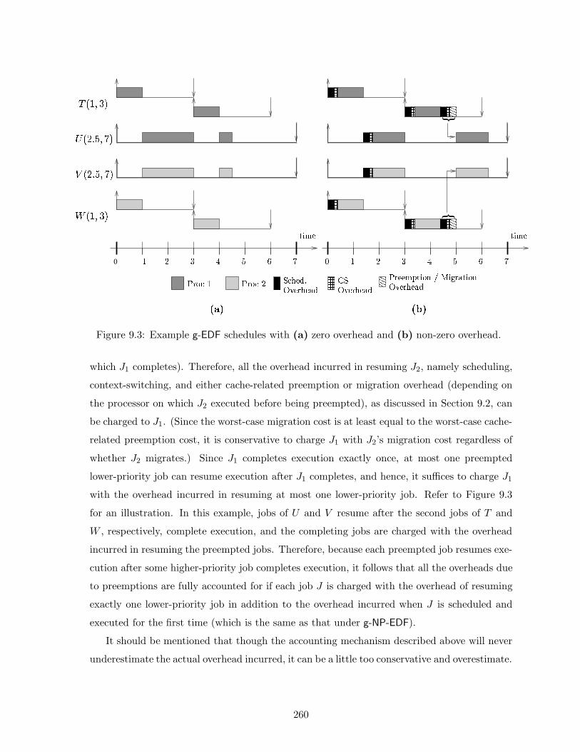
>?@@AA

BCDDEE

FGHHIIJKLLMM

NOPPQQ

RSTTUUVW

XYZZ[[

\\]]

^__

`aa

bbcc

ddeef ff fgg

{

{

0 h i j k l m n h i j o k l mo

pqrstuvwxqrstuvw

yqzu{w

|qzu{w}~�� }~��

�� }~��~��}~�� h �� i

Figure 9.3: Example g-EDF schedules with (a) zero overhead and (b) non-zero overhead.

which J1 completes). Therefore, all the overhead incurred in resuming J2, namely scheduling,

context-switching, and either cache-related preemption or migration overhead (depending on

the processor on which J2 executed before being preempted), as discussed in Section 9.2, can

be charged to J1. (Since the worst-case migration cost is at least equal to the worst-case cache-

related preemption cost, it is conservative to charge J1 with J2’s migration cost regardless of

whether J2 migrates.) Since J1 completes execution exactly once, at most one preempted

lower-priority job can resume execution after J1 completes, and hence, it suffices to charge J1

with the overhead incurred in resuming at most one lower-priority job. Refer to Figure 9.3

for an illustration. In this example, jobs of U and V resume after the second jobs of T and

W , respectively, complete execution, and the completing jobs are charged with the overhead

incurred in resuming the preempted jobs. Therefore, because each preempted job resumes exe-

cution after some higher-priority job completes execution, it follows that all the overheads due

to preemptions are fully accounted for if each job J is charged with the overhead of resuming

exactly one lower-priority job in addition to the overhead incurred when J is scheduled and

executed for the first time (which is the same as that under g-NP-EDF).

It should be mentioned that though the accounting mechanism described above will never

underestimate the actual overhead incurred, it can be a little too conservative and overestimate.

260

�� ¡¢��¡ �� £

��

¤¥¦

§¤

¤©ª«¬

«¬®°± ²®°±³

Figure 9.4: Example to illustrate that if a job of task U resumes after a job of task T completes,then U.D > T.D need not hold.

For instance, in a soft real-time system, if some job is tardy, then it is very likely that its

successor job or a job that has not yet commenced execution is scheduled when this tardy

job completes, as opposed to a preempted job of a different task. In such a scenario, the

completing job incurs no overhead associated with resuming a preempted job. Similarly, since

the total utilization of a multiprocessor-based hard real-time system scheduled under g-EDF

will be much less than 100%, the number of preemptions is likely to be much fewer than that

required for each completing job to resume a preempted job. Thus, charging each job with

the overhead incurred in resuming one lower priority job can be overkill. However, it is not

straightforward to improve the accounting mechanism without guaranteeing that tasks will

never be undercharged. We defer further investigation on this problem to future work.

Of all the overheads charged to a job of a task T , only the cache-related preemption and

migration costs are task dependent. We will now determine an upper bound for these costs.

Note that these costs depend on each task U whose jobs may resume execution after any job of

T . On a uniprocessor, it can be shown that the relative deadline of each such task U , U.D, is

larger than that of T (because, by Assumption A5, there are no early releases). However, the

same does not hold for multiprocessors. For this, consider the example in Figure 9.4. In this

example, job J2 of task U resumes immediately after job J1 of task T completes execution.

However, T.D > U.D. Thus, since no relation can be established between T and U , the worst

case is to assume that a job of a task with the largest migration overhead resumes execution

after a job of T . Hence, for all T (in the absence of other task-system-specific information), it is

necessary to charge a value of maxU∈τ∧U 6=T ohmig(g-EDF, U) to fully account for cache-related

261

overheads incurred with a preemption.

To summarize, under g-EDF, all system overheads (except that due to tick scheduling) can

be fully accounted for by inflating the WCET of each job of each task by the worst-case costs

of two scheduling decisions, two context switches, and the cost of refetching some data and

instructions evicted from the cache for one lower priority job. By the discussion above, the

following formula can be used to determine an inflated WCET for task T .

T.e = T.e(b) + 2 · ohsch(g-EDF) + 2 · ohcs(g-EDF) + max{U∈τ∧U 6=T}

(ohmig(g-EDF, U))

Tick-scheduling under g-EDF. In what follows, we describe some complexities in ensuring

that a job whose execution spans multiple, contiguous quanta is scheduled on the same pro-

cessor, and is not migrated needlessly, when a change is needed to the set of executing jobs at

a quantum boundary. Such complexities necessitate additional operations apart from a queue

merge at quantum boundaries, and hence, the overhead due to tick scheduling is likely to be

higher under g-EDF than under g-NP-EDF.5 We will use the g-EDF schedule in Figure 9.5 to

illustrate the complexities involved and some possible solutions. In this schedule, delays due

to tick scheduling are not depicted; the schedule is rather used to illustrate why additional

operations will be needed at some quanta. We will begin by considering some simple scenarios

and then move to complex ones.

In Figure 9.5, at time 1 or time 2, no new job is released. Hence, at these times, the jobs

that are executing can be resumed after brief interruptions incurred in switching to kernel

mode, verifying the status of the quantum’s release queue,6 and returning to user mode; thus,

the overhead due to tick-scheduling is limited to these operations. At time 21, task W ’s second

job, W 2, is released. Therefore, the tick-scheduling activity for time 21 requires that the kernel

on one of the processors merge the release queue with the ready queue (in addition to every

processor switching to kernel mode and testing the status of the release queue). However, the

deadline of W 2 is at time 42, and hence, W 2, which is the only job in the release queue for

time 21 (and is also the job at the head of that release queue), has lower priority than each

5It should be mentioned that some additional operations will be necessary under g-EDF even if contiguousjob executions need not be scheduled on the same processor.

6More accurately, since the first processor that finds a non-empty release queue will merge it with the readyqueue, when a processor finds an empty release queue, it must verify that no new job with higher priority is atthe head of the ready queue. For ease of description, we will refer to this operation as verifying the status ofthe release queue.

262

´ µ ¶ · ·¹ ¸º»¼½¾ ¾ ¾

¾ ¾ ¾

¿ÀÁÂÃÄ

ÅÀÃÂÆÄ

ÇÀÆÂÈÃÄ

ÉÀÊÂÁÈÄ

ËÌÌÍÎÏÐÑÍÒÓÍÒ Ôµ ¶

ÕÖÍÎ ÈÀ×ØÄ ÕÖÍÎÁ À×ÙÄFigure 9.5: Example g-EDF schedule to illustrate some complexities in ensuring that a jobwhose execution spans contiguous quanta is not migrated needlessly.

of the executing jobs and the job at the head of the ready queue (which is V 2 with deadline

at time 28). Therefore, in comparison to g-NP-EDF, the only additional operations (over a

queue merge) needed at this time are for each processor to compare the priority of its current

job (i.e., the job executing at a quantum boundary when the occurrence of a tick interrupt

invokes the scheduler) to that of the job at the head of the release queue, and to resume its

current job. Thus, the overhead incurred here is nearly the same as the worst-case overhead

incurred under g-NP-EDF.

Moving to more complex scenarios, if at a quantum boundary, some newly-released job

has higher priority than some current job, then the priority comparison described above will

not suffice: selecting the set of jobs to be scheduled in the following quantum may require

making M scheduling decisions even if the execution of some jobs will span contiguous quanta

(i.e., even if not every current job will be preempted) before a processor decides whether its

current job needs preemption. This is because if a newly-released job has higher priority than

263

some current job, then a processor whose current job’s priority is lower cannot independently

determine through a single priority comparison how many of the currently executing jobs

have higher priority than its job and whether its job should continue.7 To ensure that jobs

are not needlessly migrated, in the worst case, each processor must wait until M highest

priority jobs have been determined before identifying the job to execute on it in the next

quantum. Also, housekeeping operations associated with each current job and its task should

have been completed by its processor’s scheduler before job selections for the next quantum

can commence. Such operations include updating the job’s status to pending or complete, and

if the job is complete, enqueuing the task’s next job in the ready or the release queue.

For an illustration of the above aspects, consider times 4 and 20 in Figure 9.5, when T 2

and T 6, respectively, are released with higher priorities than any executing or ready job. If

scheduling is centralized (distributed scheduling is considered afterwards), then regardless of

which processor is the central scheduler, at time 4, the execution of V 1 has to be temporarily

stalled on processor P1 until M = 2 scheduling decisions have been made to conclude that V 1

has the second highest priority, and hence, can continue execution. Similarly, at time 20, the

executions of both U3 and V 2 should be stalled and M = 2 highest priority jobs identified

before deciding to resume U3 and preempt V 2. Also, as mentioned above, before determining

the jobs to be scheduled, the central scheduler should wait until the remaining processors have

updated the status of their current jobs, and have completed enqueue operations for next

jobs of tasks of completing jobs, if any. For instance, if P1 is the central processor, then at

time 4, unless P2 has updated the status of job U1 as complete and enqueued its next job, the

scheduling decisions of P1 may be incorrect (in that U1 may be included in the set of jobs for

time 4).8 If scheduling is distributed, wherein each processor selects one highest priority job,

then each processor should wait for all the other processors to complete making their selections

so that any job whose execution is contiguous can be correctly assigned. In the example, at

time 4, if P1 is the first processor to make a scheduling decision and selects the job with the

highest priority, and hence, chooses T 2, then unless P1 waits for P2 to select V 1 (which is the

job with the second highest priority), and does not dispatch T 2 prematurely, V 1 can migrate to

7Of course, a processor whose current job’s priority is not lower than that of the job at the head of therelease queue can safely continue executing its current job.

8The alternative of entrusting the central processor with the responsibility of updating the status of jobsrunning on other processors is likely to be cumbersome, especially when a job executes for less than its WCET, orwhen a job commences or resumes execution within a quantum (and not at a boundary) on a remote processor.

264

P2. Furthermore, as with the centralized case, each processor should wait for other processors

to complete updating the status of their current jobs before making its selection, and thus,

tick scheduling may require two passes. Finally, mechanisms will be needed to ensure that

the current jobs are considered efficiently along with those in the ready queue while making

scheduling decisions. For instance, consider time 20, when both the executing jobs have to be

considered along with T 6, the job merged onto the ready queue, in deciding which jobs run

during [20, 21).

g-EDF implementation. We now describe one possible approach, which is distributed, for

efficiently ensuring that all possible complexities are handled and needless job migrations are

eliminated. We propose ordering the processors such that each processor can make just one

selection, and yet, dispatch the job it selects without waiting for the remaining processors to

complete their selections. (In other words, the proposed processor order can ensure that each

current job that will execute in the next quantum is selected by its current processor.) This

processor order is given by the reverse priority order of the processors’ current jobs that will

not complete by the end of the current quantum (and hence will be eligible and contend for

execution in the next quantum)9 and is maintained in a reverse priority queue called a running

queue. A processor that is idle, or whose current job will complete by the end of the current

quantum, will have a dummy or placeholder job with the lowest priority to represent it in the

running queue.

Given this running queue data structure, while making selections at the next quantum

boundary, each processor should wait for its dummy or current job to be at the head of the

running queue. If it has a dummy job at the head, then the processor simply selects the job

(if any)10 at the head of the ready queue for execution on it; else, the processor selects either

its current job or the job at the head of the ready queue, depending on which job has higher

priority, resolving any tie in favor of its current job. In either case, the processor deletes its

entry (current or dummy job) from the current running queue, and enqueues its new entry in

the running queue for the next quantum. Since a processor that is idle or whose current job

will not be pending at the next quantum has no constraints on selecting a newly-released job,

letting such a processor select a highest priority job from the ready queue before processors

9For now, assume that each job executes for its WCET. Handling premature job completions is addressedbelow.

10If the ready queue is empty, then the processor will idle during the next quantum.

265

whose jobs may continue execution is appropriate. In a similar vein, since the running queue

is ordered by non-decreasing priority and has one entry for each processor, if a processor’s

current (not dummy) job reaches the running queue’s head and has lower priority than that

currently at the head of the ready queue, then this job is guaranteed to be not scheduled

in the next quantum, and so, deleting it from the running queue (after enqueuing it in the

ready queue) is appropriate. Finally, running queues of at most two consecutive quanta will

be needed at any time, and so, maintaining just two queues and switching their roles at every

quantum suffices. (In other words, queues for the different quanta can be maintained as a

circular queue of queues of length two.)

The above approach can be made to be robust in the face of jobs not executing for their

full WCET as follows. To account for the case wherein jobs complete early exactly at quantum

boundaries, a pre-scheduling phase or pre-phase, in which processors of such jobs make their

selections before the remaining processors, can be included. Processors selecting during the pre-

phase will not select during the regular phase; the regular phase can commence after processors

have reached consensus (e.g., through barrier synchronization) that they are through with the

pre-phase. On the other hand, if a job’s early completion is within a quantum (as opposed to a

quantum boundary), then when the scheduler is invoked at the early completion time11 and a

new job is selected, the processor can modify its entry in the ready queue to correspond to the

newly-scheduled job or a dummy job (by changing the entry’s priority and other details such as

task and job identifiers) in O(lg M) time (assuming a binomial or binary heap implementation).

One important caveat of the above approach, however, is that if quanta are not aligned on

processors, then to ensure both minimal processor waiting times and scheduling contiguous

job executions on the same processor, scheduling may have to be centralized, with the first

processor arriving at the beginning of a logical quantum serving as the central processor.

Hence, additional synchronization and other mechanisms will be needed to communicate early

job completions, wherein jobs execute for less than their WCETs, to the central scheduler (to

account for scenarios in which the central scheduler makes selections assuming that a job will

continue, whereas the job completes early after the scheduler’s decision).

Though the complexities described above will have to be addressed only at those quanta at

which new jobs that have higher priority than one or more of the executing jobs are released,

and hence, the number of “complex” quantum boundaries is bounded by the number of jobs,

11The amount of time elapsed since the beginning of that quantum can be determined with high precisionusing high-resolution timing devices such as the Pentium R© Time-Stamp Counter of Intel R©.

266

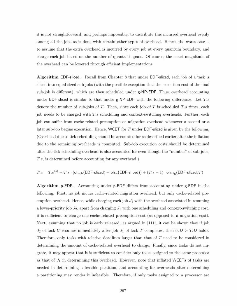
it is not straightforward, and perhaps impossible, to distribute this incurred overhead evenly

among all the jobs as is done with certain other types of overhead. Hence, the worst case is

to assume that the extra overhead is incurred by every job at every quantum boundary, and

charge each job based on the number of quanta it spans. Of course, the exact magnitude of

the overhead can be lowered through efficient implementations.

Algorithm EDF-sliced. Recall from Chapter 8 that under EDF-sliced, each job of a task is

sliced into equal-sized sub-jobs (with the possible exception that the execution cost of the final

sub-job is different), which are then scheduled under g-NP-EDF. Thus, overhead accounting

under EDF-sliced is similar to that under g-NP-EDF with the following differences. Let T.s

denote the number of sub-jobs of T . Then, since each job of T is scheduled T.s times, each

job needs to be charged with T.s scheduling and context-switching overheads. Further, each

job can suffer from cache-related preemption or migration overhead whenever a second or a

later sub-job begins execution. Hence, WCET for T under EDF-sliced is given by the following.

(Overhead due to tick-scheduling should be accounted for as described earlier after the inflation

due to the remaining overheads is computed. Sub-job execution costs should be determined

after the tick-scheduling overhead is also accounted for even though the “number” of sub-jobs,

T.s, is determined before accounting for any overhead.)

T.e = T.e(b) + T.s · (ohsch(EDF-sliced) + ohcs(EDF-sliced)) + (T.s − 1) · ohmig(EDF-sliced, T )

Algorithm p-EDF. Accounting under p-EDF differs from accounting under g-EDF in the

following. First, no job incurs cache-related migration overhead, but only cache-related pre-

emption overhead. Hence, while charging each job J1 with the overhead associated in resuming

a lower-priority job J2, apart from charging J1 with one scheduling and context-switching cost,

it is sufficient to charge one cache-related preemption cost (as opposed to a migration cost).

Next, assuming that no job is early released, as argued in [111], it can be shown that if job

J2 of task U resumes immediately after job J1 of task T completes, then U.D > T.D holds.

Therefore, only tasks with relative deadlines larger than that of T need to be considered in

determining the amount of cache-related overhead to charge. Finally, since tasks do not mi-

grate, it may appear that it is sufficient to consider only tasks assigned to the same processor

as that of J1 in determining this overhead. However, note that inflated WCETs of tasks are

needed in determining a feasible partition, and accounting for overheads after determining

a partitioning may render it infeasible. Therefore, if only tasks assigned to a processor are

267

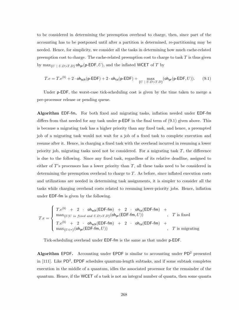
to be considered in determining the preemption overhead to charge, then, since part of the

accounting has to be postponed until after a partition is determined, re-partitioning may be

needed. Hence, for simplicity, we consider all the tasks in determining how much cache-related

preemption cost to charge. The cache-related preemption cost to charge to task T is thus given

by max{U | U.D>T.D} ohpr(p-EDF, U), and the inflated WCET of T by

T.e = T.e(b) + 2 · ohsch(p-EDF) + 2 · ohcs(p-EDF) + max{U | U.D>T.D}

(ohpr(p-EDF, U)). (9.1)

Under p-EDF, the worst-case tick-scheduling cost is given by the time taken to merge a

per-processor release or pending queue.

Algorithm EDF-fm. For both fixed and migrating tasks, inflation needed under EDF-fm

differs from that needed for any task under p-EDF in the final term of (9.1) given above. This

is because a migrating task has a higher priority than any fixed task, and hence, a preempted

job of a migrating task would not wait for a job of a fixed task to complete execution and

resume after it. Hence, in charging a fixed task with the overhead incurred in resuming a lower

priority job, migrating tasks need not be considered. For a migrating task T , the difference

is due to the following. Since any fixed task, regardless of its relative deadline, assigned to

either of T ’s processors has a lower priority than T , all these tasks need to be considered in

determining the preemption overhead to charge to T . As before, since inflated execution costs

and utilizations are needed in determining task assignments, it is simpler to consider all the

tasks while charging overhead costs related to resuming lower-priority jobs. Hence, inflation

under EDF-fm is given by the following.

T.e =

T.e(b) + 2 · ohsch(EDF-fm) + 2 · ohcs(EDF-fm) +max{U |U is fixed and U.D>T.D}(ohpr(EDF-fm, U)) , T is fixed

T.e(b) + 2 · ohsch(EDF-fm) + 2 · ohcs(EDF-fm) +max{U∈τ}(ohpr(EDF-fm, U)) , T is migrating

Tick-scheduling overhead under EDF-fm is the same as that under p-EDF.

Algorithm EPDF. Accounting under EPDF is similar to accounting under PD2 presented

in [111]. Like PD2, EPDF schedules quantum-length subtasks, and if some subtask completes

execution in the middle of a quantum, idles the associated processor for the remainder of the

quantum. Hence, if the WCET of a task is not an integral number of quanta, then some quanta

268

may be partially wasted, and thus, in comparison to the algorithms considered above, EPDF

can incur an additional overhead. This overhead can be accounted for by rounding each task

execution cost (obtained after accounting for the remaining overheads) up to the next integer,

and hence is referred to as rounding overhead .

Rounding overhead also necessitates the use of an iterative formula for determining the

overall inflation needed for each task. To see this, let T.e(0) def= T.e(b) denote the base WCET

of T . Then, the number of scheduling decisions needed for each job of T is dT.e(0)e. Similarly,

since each job may be preempted at the end of every quantum, a safe upper bound on the

number of preemptions is dT.e(0)e − 1. Hence, the number of context switches and migrations

(because each preemption may result in a migration) to account for are dT.e(0)e and dT.e(0)e−1,

respectively. Accounting for these, we arrive at T.e = T.e(0) + dT.e(0)e · (ohsch(EPDF) +

ohcs(EPDF)) + (dT.e(0)e − 1) · ohmig(EPDF, T ), and accounting for the rounding overhead, we

have T.e = dT.ee. Note that if dT.ee is different from dT.e(0)e then our inflation may not

be safe and has to be revised by substituting T.e for T.e(0) within the ceiling operators to

arrive at a new estimate for T.e. The procedure has to be repeated iteratively either until

convergence is reached or T.e = T.p, whichever is earlier. An iterative formula for this is given

below. In this formula, T.e(k) denotes the WCET after the kth iteration. As mentioned earlier,

T.e(0) = T.e(b). (It is assumed that the units for the overhead costs are quanta and can be

non-integral.)

T.e(k+1) =⌈

T.e(b) + dT.e(k)e · (ohsch(EPDF) + ohcs(EPDF)) + (dT.e(k)e − 1) · ohmig(EPDF, T )⌉

Expressed another way, T ’s inflated WCET T.e under EPDF is given by

T.e = min(

T.p,(

min t : t =⌈

T.e(b) + dte · (ohsch(EPDF) + ohcs(EPDF)) + (dte − 1) · ohmig(EPDF, T )⌉))

A difference in the above formula with respect to that provided in [111] for PD2 is in the

last term. Under PD2, since no deadlines are missed, a better estimate on the number of

preemptions is possible by noting that each job of T completes execution within T.p quanta

of its release. Hence, if T.p < 2 · T.e, then each job of T can be preempted at most T.p − T.e

times, which is at most T.e − 1. Thus, the number of preemptions under PD2 is bounded by

min(T.e−1, T.p−T.e). However, since deadlines can be missed under EPDF, each job of T may

269

not complete until before T.p + q quanta after its release, where q is a tardiness bound for the

task system under consideration. Therefore, only a weaker bound of min(T.e−1, T.p+q−T.e)

on the number of preemptions can be shown to hold under EPDF.12 However, since a bound

on q requires a bound on the maximum task weight, which in turn depends on the overheads,

for simplicity, we just use the looser bound of T.e − 1.

9.4 Performance Evaluation

In this section, we present the results of experiments conducted to evaluate the algorithms

considered in this dissertation and p-EDF. In these experiments, base WCETs and periods for

tasks were generated randomly. On the other hand, overhead costs were assigned based on

measurements obtained from an experimental test-bed containing prototype implementations

of the algorithms. As mentioned earlier, our objective is to evaluate the algorithms with respect

to the percentage of task sets for which bounded tardiness can be guaranteed and the range

for the guaranteed bounds. We first describe the procedure used to select overhead costs. The

procedure used to generate task sets and the results of the evaluation are presented afterwards.

9.4.1 Estimation of Overheads

Worst-case values for the overheads described in Section 9.2 were measured using an experimen-

tal prototype called LITMUSRT. LITMUSRT stands for LInux Testbed for MUltiprocessor

Scheduling in Real-Time systems and its current version was developed in collaboration with

Calandrino et al. [41], with facilitating comparison of real-time scheduling algorithms on a

multiprocessor as one of its purposes.

LITMUSRT was not built from scratch, but rather by modifying Linux such that its

underlying scheduler is configurable at boot time. This was facilitated by modularizing the

Linux scheduler so that a new algorithm can be plugged in easily. Currently, implementations

are available for g-EDF, g-NP-EDF, p-EDF, PD2, and two variants of PD2. Further details on

LITMUSRT and its implementation can be found in [41]. Some relevant aspects are as follows:

to ensure that all sources of unpredictability are eliminated, paging is disabled; further, all

pages are locked in memory, and all real-time tasks are restricted to sharing a common address

space. LITMUSRT currently runs on the 2.6.9 version of the Linux kernel. Our measurements

12It should be pointed out that the bound derived for PD2 can be shown to hold under EPDF asymptotically(that is, over long periods) for periodic task systems.

270

were performed on an SMP consisting of four 32-bit Intel R© Xeon R© processors running at 2.7

GHz with 2GB memory. Each processor had 8K instruction and data caches, and a unified

512K L2 cache. Cache lines were 64 bytes wide.

Cache-related preemption and migration costs. Recall that a worst-case scenario for

cache-related delays due to preemptions and migrations occurs when each processor has some

preempted task resuming on it, and each is refetching data and/or instructions evicted from

the cache. Also note that the actual delay depends on the code and working-set sizes (WSSs)

of the tasks. Hence, we determined worst-case preemption and migration costs for five WSSs of

4K, 32K, 64K, 128K, and 256K (in an attempt to estimate these costs for systems with varying

data dependencies). (While the WSSs considered may appear to be small, these represent the

amount of data that a task fetches at the beginning of a quantum, typically within one ms,

concurrently with every other processor, and it is not possible to read a much larger amount

of data in that time. On the other hand, if a preemption may cause much larger working sets

to be lost from the cache and much higher contention, then preemptive algorithms may not

be appropriate for the underlying application.)

Worst-case costs were determined by emulating worst-case scenarios. To emulate worst-

case preemptions, we let each processor write a block of memory of a specified size at the same

time. The time taken for the write to complete, less the time taken to write the same amount

of data in the same scenario, but with all written data being locally cached, was taken as an

estimate of the worst-case preemption cost. Migration costs were measured similarly, but by

including the emulation of migration of data from one cache to another. This was done by

reading data into the cache of one processor, and then writing that same data on a second

processor. This had the effect of bringing the data into the cache of the second processor,

while invalidating it in the cache of the first processor. The amount of time taken for the

second processor to write its working set (less the time taken to write the same amount of

data resident in cache as was done with preemption costs) was taken as an upper bound on

the worst-case migration cost. Preemption costs for the five WSSs considered were found to

be 16µs, 67µs, 115µs, 230µs, and 439µs, while migration costs were 16µs, 68µs, 126µs, 272µs,

and 561µs.

Since our measurements were on a four-processor system, in our simulation studies, we

used the above costs for experiments on four processors. We expect contention on the shared

bus to increase at most linearly with the number of processors, so for an arbitrary number

271

M of processors, where M ∈ {2, 4, 8, 16}, we scaled the above costs linearly. Specifically, if x

denoted the cost on four processors, then the cost on M processors was taken as Mx/4. (The

discrepancies, if any, in costs thus computed for M 6= 4 from the actual costs that can be

observed on an M processor system remain to be determined.)

Context-switching overhead. Context-switching overhead was measured by recording the

times before and after a context-switch call assuming that all processors perform a context

switch concurrently. This cost was found to be of the order of 0.5µs for p-EDF, and 1µs for

the remaining algorithms. For all the algorithms, in comparison to the other costs, the cost of

a context switch was thus negligible.

Scheduling overhead. In assigning scheduling costs, we assumed all tasks to be periodic. In

the current version of LITMUSRT, priority queues are implemented using linked lists (which

are not the most efficient way for implementing priority queues). Further, the implementation

of g-EDF is not efficient. We considered these to be limiting, and hence, did not use LITMUSRT

to measure scheduling costs. Rather, we approximated scheduling costs by measuring times in a

binomial heap implementation. The predominant cost in making a scheduling decision consists

of switching to kernel mode, enqueuing the completing job’s next instance or the preempted job

in a release queue or the ready queue, merging the ready queue and a release (or the pending

queue), and dequeuing the highest-priority task from the ready queue. Hence, we measured

the total time taken to perform these operations in our binomial heap implementation. The

heap node contained all the fields that would be present in a priority-queue node of a scheduler.

A cold cache was ensured before each fresh set of operations (enqueue, merge, and extract)

was performed.

We measured the average time taken to perform the entire set of operations described

above, including the time taken to switch to kernel mode, for n ranging from ten to 2000,

where n denotes the number of nodes. For each n, the average time taken was between 2.0µs

and 3.0µs, of which approximately 0.75µs is the time taken to switch to kernel mode. Since

the worst-case time complexity of all the operations of interest to us is O(lg n) when a binomial

heap is used, we (somewhat arbitrarily) fixed the cost of a scheduling decision for a queue size

of n on a single processor as 2.0 + lg n · 0.125µs = 0.75 + 1.25 + lg n · 0.125µs. (The actual

reasoning behind the second term is as follows. lg n increases approximately by 8 as n increases

from 10 to 2000. Hence, since the measured time increased by 1000ns as n increased from 10

272

to 2000, it seemed appropriate to increase the total cost by 1000/8 = 125ns as lg n increases

by one.) Thus, for p-EDF and EDF-fm, since the number of tasks per processor is N/M on

average, a cost of 2.0 + lg NM · 0.125µs was charged.

We next describe the cost assigned to global algorithms and the reasoning behind it. Global

algorithms use a shared queue and are restricted to accessing it in a mutually-exclusive manner.

Scheduling is either centralized , with a single central processor making scheduling decisions for

all the processors as with Pfair algorithms, or distributed , with each processor making its own

scheduling decision. Either way, in the worst case, each processor is delayed by the time taken

to make M −1 scheduling decisions, and hence, for global algorithms, we charged a scheduling

cost of 0.75+ M · (1.25+ lg n · 0.125)µs per scheduling decision. Compare this expression with

the one provided above for partitioned algorithms. The 0.75µs term in this expression accounts

for the time taken to switch to kernel mode. Since each processor can switch to kernel mode

independently, and is not delayed by other processors, this cost need not be multiplied by M .

We ignored queue-based spin lock acquisition times, as these were measured to be minimal

(of the order of nanoseconds).13 Also, since measurements were made with a cold cache,

the migration of priority-queue nodes from one cache to another is accounted for. Further,

measurements with scheduler implementations on LITMUSRT show that in comparison to

p-EDF, the cost of a scheduling decision is higher under global algorithms by less than 1 µs

(except under g-EDF, whose LITMUSRT implementation is not efficient). Hence, we believe

that our accounting for global algorithms is safe by a wide margin.

Overhead due to tick scheduling. For all non-Pfair algorithms considered, except g-EDF,

the predominant cost incurred due to tick scheduling is the time taken to switch to kernel

mode, and merge a release queue or the pending queue with the ready queue. This cost was

measured to be almost the same as the scheduling cost described above, and hence, we charged

2.0 + lg n · 0.125µs for g-NP-EDF and EDF-sliced, and 2.0 + lg NM · 0.125µs for p-EDF and EDF-

fm. For global algorithms, since at most one processor performs a merge, and lock acquisition

times within the kernel (after switching to kernel mode) are negligible, per-processor delays

are negligible. Hence, there is no term accounting for per-processor delays. Under g-EDF, to

13Typically, synchronization within the kernel is by disabling interrupts, or by “busy waiting,” also known asspinning . Disabling interrupts is not effective (i.e., cannot guarantee mutual exclusion) on multiprocessors andsimple spinning cannot guarantee predictable waiting times and can cause excessive traffic on the interconnect.Queue-based spin locks [89] lower interconnect traffic by having each process spin on a variable that is localto it, and hence, each spin variable can be cached. Predictability is ensured by including mechanisms to orderspinning processes in a FIFO manner and by enabling their spin variables in that order.

273

ensure that jobs whose executions span contiguous quanta are not migrated, in the worst case,

apart from one merge by any of the processors, each processor may have to wait for every

other processor to update the status of its current job, and perform one enqueue and dequeue

operation, and hence, we charged 0.75 + M · (1.25 + lg n · 0.125)µs as the tick-scheduling cost

for g-EDF. (As with the scheduling overhead, the term 0.75µs corresponds to the time taken

to switch to kernel mode, and since each processor can switch to kernel mode independently

and is not delayed by any of the remaining processors, this term is not multiplied by M .)

9.4.2 Experimental Setup

We are now ready to describe our simulation procedure. Since the processors-to-memory

interconnection can be quite different and need not be a bus when the number of processors is

greater than 16, we do not believe that overheads measured on a four-processor system can be

extrapolated to systems with greater than 16 processors. Hence, in our simulations we limited

M to be at most 16. Simulations were performed for each combination of the parameters listed

below for algorithms p-EDF, g-EDF, g-NP-EDF, EDF-fm, EDF-sliced, and EPDF. (PD2 was not

included as overheads under it are almost the same as that under EPDF.) As mentioned earlier,

each task set was assumed to be periodic. In our LITMUSRT implementation, all tasks share

a single address space, and hence, we assume this for our experiments. as Under EDF-sliced,

jobs were sliced such that the base execution cost of each sub-job (except that of a job’s last

sub-job) was integral and at least two quanta. The parameters below were chosen so that

the two conflicting goals of ensuring that scenarios that arise in practice are covered and of

maintaining a manageable simulation process are both reasonably met. Overhead costs were

based on measurements described in the previous section.

• M in {2, 4, 8, 16};

• quantum size Q in {500µs, 1000µs, 5000µs};

• base task utilization limits, [umin, umax), in {[0.1, 0.5), [0.3, 0.7), [0.5, 0.9), [0.1, 0.9)};

• task period limits, [pmin, pmax), in {[10, 100), [100, 500)};

• preemption and migration costs, denoted as a pair, in {(4Mµs, 4Mµs), (29Mµs, 32Mµs),

(58Mµs, 68Mµs)} for WSSs of 4K, 64K, and 128K respectively; (all tasks of a task set

274

were assigned equal preemption and migration costs);14

• context-switching cost fixed at 2.0µs;

• scheduling cost set to 2.0 + lg( NM ) · 0.125µs for p-EDF and EDF-fm and to 0.75 + M ·

(1.25 + lg(N) · 0.125)µs for the remaining algorithms;

• overhead due to tick scheduling set to 2.0 + lg( NM ) · 0.125µs for p-EDF and EDF-fm, to

2.0+lg N ·0.125µs for g-NP-EDF and EDF-sliced, and to 0.75+M ·(1.25+lg(N) ·0.125)µs

for g-EDF.

Quantum size was primarily varied to determine the impact on EPDF and EDF-sliced. Recall

that either quantum-length subtasks, or sub-jobs (of uniform size that is at least one quantum

and that can be chosen arbitrarily) are scheduled under these algorithms. Hence, scheduling

and migration overheads are lowered as quantum size is increased. On the other hand, for

EPDF, rounding error can increase. (Since tick-scheduling overhead is less in comparison to

other overheads, we do not expect the remaining algorithms to be impacted much.)

The range for task periods was varied for a similar reason. For a given base task utilization,

a larger period implies a larger base execution cost. Since under the non-Pfair algorithms

considered, the number of preemptions is at most the number of jobs, and all overhead, except

the tick-scheduling overhead, charged to a job is independent of the job size, the overhead cost

per base unit of execution decreases with increasing execution costs.

For each combination of the parameters listed above (referred to as a run), a certain

number of random task sets was generated. (The exact number is discussed later.) The task set

generation procedure was as follows. For each new task set, M+1 tasks were initially generated.

Each task’s period and utilization were distributed uniformly in the range [pmin, pmax) and

[umin, umax), respectively. Tasks were added one at a time to the initial task set as long as

the base total utilization was less than M . Upon addition of each new task, overheads were

determined, and a tardiness bound was computed if the inflated utilization, after accounting

for the overheads, was less than M . (The addition of tasks terminated when the inflated

utilization exceeded M .) Thus, schedulability was determined for several subsets of the entire

task set. The total number of complete (or independent) task sets generated depended on the

per-task utilization range, and was limited to 30,000, 45,000, 60,000, and 45,000, in that order,

for the four ranges listed earlier. These numbers were chosen after some trial-and-error so

14There was no noticeable difference in the results if these costs differed slightly for different tasks.

275

that enough task sets were generated for each base total utilization. The number of generated

task sets had to be varied with the per-task utilizations to ensure that a sufficient number

of task subsets with lower total utilizations were generated even when per-task utilizations

were high. (Note that when the utilization of each task is at least 0.5, with M + 1 tasks,

the base total utilization is at least (M + 1)/2.) In computing inflated WCETs, the formulas

provided in Section 9.2 were used. The total number of task sets (including subsets) that each

algorithm could schedule15 was determined for each run and is plotted against varying total

base utilizations. Under p-EDF, the first-fit decreasing heuristic (in which tasks are considered

in non-increasing order of their utilizations) was used for partitioning tasks among processors,

and under EDF-fm, the LEF (resp., LUF) task assignment heuristic was used when umax (after

inflation) was at most 0.5 (resp., exceeded 0.5). (Recall from Chapter 5 that LEF guaranteed

the lowest tardiness if an assignment under it was possible and LUF could assign the maximum

number of task sets with umax > 0.5.) The average of the tardiness bound guaranteed was

also computed for each algorithm, and is also plotted against varying base utilizations. In

computing the average tardiness bounds, only schedulable task sets were included. Hence, the

tardiness results should be used only in conjunction with the schedulability results.

9.4.3 Experimental Results

Graphical plots of the results of the simulation runs described above are presented in the

following manner.16 As mentioned above, two graphs were generated for each run. The x axis

represents the total base task system utilization in both the graphs; the y axis represents the

number of task sets in the first graph, and the mean of maximum tardiness, normalized with

respect to the average execution cost, in the second graph. The first graph plots the total

number of task sets generated and the number found to be schedulable under each algorithm,

while the second graph plots the mean normalized tardiness for each algorithm, considering

only schedulable task sets. For example, if Algorithm A could guarantee bounded tardiness

to 1000 task sets in some run, whereas Algorithm B could do so for only 10 task sets in the

same run, then the tardiness bounds plotted for A and B are averages of the tardiness bounds

computed for the 1000 and 10 schedulable task sets, respectively. Therefore, a lower tardiness

bound plotted for B does not imply that B is necessarily “better,” and hence, as mentioned

15In the rest of this chapter, at the risk of abusing terminology, we refer to a task set that can be guaranteedbounded tardiness under Algorithm A as schedulable under A.

16Plots in which M = 16 or Q = 500µs have been omitted to limit the amount of data presented.

276

above, tardiness results should not be considered independent of schedulability results. 99%

confidence intervals are shown in the second graph. (99% confidence intervals were determined

for the plots in the first graph also, but have been omitted as their ranges are minimal, and

their inclusion obscures the identification marks of the different curves.)

The generated graphs are grouped as follows. Four graphs, one each for each task utilization

range, and equal values for the remaining parameters (such as periods, quantum size, etc.),

are grouped and are shown in a common figure in a single page. In each figure, all four graphs

(or insets (a) through (d)) plot either the number of schedulable task sets or the mean of

the maximum tardiness. The task utilization range is the lowest for inset (a), highest for

inset (c), and in between for inset (b). In inset (d), task utilizations span the range [0.1, 0.9),

which includes the ranges of the other three insets. For each set of parameters, the figure with

schedulability plots is presented first followed by the figure with tardiness plots. This should

facilitate comparing the tardiness bounds to the percentage of task sets for which the bound

is applicable. It should be noted that since the tardiness bounds plotted are average values

computed considering only schedulable task sets, a drop (which may seem counterintuitive)

can be observed with increasing base utilization for some algorithms, most notably for EDF-fm

(discussed further later). This drop is due to a steep decrease in the number of schedulable

task sets. For the same reason, as described above, a lower tardiness bound does not imply

better overall performance. Another aspect that needs explanation is the variation in the shape

of the “Total Task Sets” curve, and hence, those of the other curves, with varying per-task

utilizations. Note that in almost every figure with schedulability plots, the “Total Task Sets”

curve is a straight line in inset (a) (i.e., for low per-task utilizations), and is in general (except

at the extreme end) a non-decreasing function of the base total utilization in insets (b)–(d).

This variation is due to the difficulty in generating sufficient number of task sets with low base

total utilizations when per-task utilizations are high, as explained earlier.

Figures are presented in increasing order of M . For each choice of M , figures are shown

for the three preemption and migration costs, and the two period ranges considered. In what

follows, we discuss performance trends exhibited by the algorithms as parameters are varied.

Impact of task utilizations. To study the impact of task utilizations, we will consider

the results in Figures 9.6 and 9.7. For the runs here, M = 2, and preemption and migration

costs are the lowest (of those considered). Referring to inset (a) of Figure 9.6, when task

utilizations are low, schedulability is 100% for all the algorithms even when the total base

277

utilization exceeds 75%. In this inset, schedulability drops first for EPDF, followed by p-EDF

and EDF-sliced in that order. The remaining three algorithms (g-EDF, g-NP-EDF, and EDF-fm)

could schedule 100% of the task sets even when the base load is 90%. However, because g-NP-

EDF does not suffer from job preemptions or migrations, and EDF-fm incurs lower scheduling

overhead, these two algorithms perform better than g-EDF by over 25% when the base load is

95%. The main difference between EPDF and EDF-sliced is in the absence of rounding overhead

for the latter, and hence, the difference in the schedulabilities of these two algorithms is a rough

indicator of the loss due to rounding. Similarly, since preemption costs are minimal here, the

loss suffered by p-EDF is primarily due to an inability to feasibly partition a task set. Note

that even when both task utilizations and preemption costs are low, which is the best case for

p-EDF, g-NP-EDF and EDF-fm perform better than p-EDF by over 50%, and g-EDF performs

better by 20%, when the total load is 1.9, which is near the maximum allowed.

As we move to inset (b), schedulability decreases for p-EDF, and in inset (c), it drops to close

to 0%. However, there is no significant change for the remaining algorithms. (As mentioned

earlier, the variations in the shapes of the “Total Task Sets” curve and other curves with per-

task utilization ranges is due to the variation in the total number of task sets generated for

each base total utilization, and do not indicate differences in schedulability.) Note that EDF-

fm performs strikingly well even with high task utilizations. This is due to fact that M = 2

here, and on two processors, all feasible task systems can be successfully assigned (refer to

Chapter 5).

Considering the tardiness bounds guaranteed by the algorithms, the three algorithms with

higher schedulability suffer from higher tardiness as well. p-EDF performs well only when

per-task and total utilizations are both low. However, this is not an interesting scenario.

EPDF performs well (when migration costs are low to moderate) even when total utilization

is moderately high regardless of task utilizations. On the other hand, if per-task or total

utilization or both are high, g-EDF, g-NP-EDF, or EDF-fm may be used depending on tardiness

tolerance limits. Referring to inset (a) of Figure 9.7, at low task utilizations, tardiness is lowest

for EDF-fm; when task utilizations are high, g-EDF performs better. In all cases, schedulability

is highest for g-NP-EDF, implying that g-NP-EDF may be the only choice for some task systems.

Similar trends are observed for all of the algorithms except EDF-fm in the other figures

also, that is, when task utilizations are varied for other values (than considered above) of the

remaining parameters also. (Note that we are referring only to the changes observed among the

insets in one of Figures 9.19–9.43, and not to the changes between two different figures.) For

278

M > 2, schedulability drops significantly for EDF-fm when moving from inset (b) to inset (c),

that is, when all tasks are heavy. For example, refer to insets (b) and (c) of Figure 9.19. Note

that the performance of EDF-fm is significantly better than that of p-EDF in insets (b) and (d),

even though not all tasks are light in these task sets. (Recall from Chapter 5 that bounded

tardiness is guaranteed under EDF-fm only if all tasks are light.)

Two trends warrant explanation in the tardiness figures. First, tardiness plots are not

smooth for g-EDF and g-NP-EDF for any M , but contain jumps. The expressions for tardiness

bounds for these algorithms contain bUsumc as part of the upper limit of the summation in the

first term of the numerator and the second term of the denominator, and hence, the tardiness

bound changes abruptly at each integral value of Usum. Since Usum denotes the total inflated

utilization and the plots are against the total base utilization, which is less than the inflated

utilization, abrupt jumps can be observed at non-integral values of the total base utilization.

(The next integral value would represent the corresponding total inflated utilization.) The

second trend of interest is that when M > 2, the tardiness bound for EDF-fm is not strictly non-

decreasing in insets (b) and (c), and in some cases in inset (d). Specifically, some undulations

can be observed in insets (b) and (d), and a steep drop when the total base utilization is in

the 80%-85% range in inset (c). In insets (b)–(d), the maximum inflated utilization of a task

exceeds 0.5, and hence, the LUF heuristic is used for task assignment for task sets in these insets.

We surmise that the undulations, and to some extent, the steep drop, are due to the uniform

distribution of the spare capacity among the processors when assigning tasks. Hence, as the

base total utilization is only slightly increased, a slightly higher percentage of each processor’s

capacity is made available for assignment to tasks, and so, for a given per-task utilization

range, it may be possible to lower the utilizations of migrating tasks in comparison to when

the total base utilization is slightly lower. Since the tardiness bound under EDF-fm increases

with the utilizations of the migrating tasks, a decrease in the tardiness bound can ensue. To

see this, suppose that a task system’s maximum inflated per-task utilization and total inflated

utilization are 0.8 and 0.75M, respectively. Then, because the distribution of spare capacity

across processors is uniform, each processor is utilized only up to 75%. Hence, no task with

utilization exceeding 0.75 can be assigned as a fixed task. On the other hand, if the total

utilization is increased to 0.8M, then since the total utilization on each processor can be up to

80%, and under LUF, fixed tasks are assigned in the order of non-increasing utilizations, there

is a significantly higher scope for tasks with utilizations in the range (0.75, 0.8] to be assigned

as fixed tasks. On the other hand, task assignment becomes harder as the total utilization

279

increases, and so, whether tardiness increases or decreases depends on which of the two factors

dominates as the base total utilization is slightly increased, and can be arbitrary and difficult

to explain around certain points. We also surmise that the tardiness plots will be smoother

if the task assignment heuristic is modified so that the uniform distribution of spare capacity

guideline is relaxed to facilitate assigning heavier tasks as fixed tasks. The steep drop in the

tardiness bound in inset (c) could additionally be due to the deep plunge in schedulability

that accompanies at the corresponding point. Recall that the tardiness bound plotted is the

average computed for schedulable task sets only.

Bimodal distribution for task utilizations. In all the schedulability figures, when all

tasks are heavy (i.e., in inset (c)), even EPDF and EDF-sliced — the algorithms that incur

the most overhead — perform better than p-EDF and EDF-fm. However, since the practical

significance of task systems composed exclusively of heavy tasks is not known, we also de-

termined the schedulability for task systems that are not exclusively but only predominantly

heavy, by including a few light tasks using a bimodal distribution for task utilizations, dis-

tributed between the ranges [0.1, 0.5) and [0.5, 0.9) with probabilities 0.1 and 0.9, respectively.

Schedulability results for this bimodal distribution for task utilizations are available in Fig-

ures 9.18, 9.31, and 9.44, for M = 2, M = 4, and M = 8, respectively. Though schedulability

is much higher for p-EDF and EDF-fm in these figures than when all tasks are heavy, EPDF

and EDF-sliced are still always better than p-EDF, and are better than EDF-fm in most cases.

Schedulability can be expected to improve for p-EDF and EDF-fm as the percentage of light

tasks is increased and deteriorate for EPDF and EDF-sliced. Insets (d) of the schedulability

figures, in which task utilizations are uniformly distributed in [0.1, 0.9), correspond to the case

when the percentages of light and heavy tasks are nearly equal.

280

0

2000

4000

6000

8000

10000

1 1.1 1.2 1.3 1.4 1.5 1.6 1.7 1.8 1.9

Num

ber

of S

ched

ulab

le T

ask

Set

s

Total Utilization (Base)

Schedulable Task Sets by Total Util. (M=2)

Total Task Setsg-EDF

g-NP-EDFEDF-Sliced

EDF-fmEPDF

P-EDF

(a)

0

2000

4000

6000

8000

10000

1 1.1 1.2 1.3 1.4 1.5 1.6 1.7 1.8 1.9

Num

ber

of S

ched

ulab

le T

ask

Set

s




g-NP-EDFEDF-Sliced

EDF-fmEPDF

P-EDF

(b)

0

2000

4000

6000

8000

10000

1.35 1.4 1.45 1.5 1.55 1.6 1.65 1.7 1.75 1.8 1.85 1.9

Num

ber

of S

ched

ulab

le T

ask

Set

s




g-NP-EDFEDF-Sliced

EDF-fmEPDF

P-EDF

(c)

0

2000

4000

6000

8000

10000

1 1.1 1.2 1.3 1.4 1.5 1.6 1.7 1.8 1.9

Num

ber

of S

ched

ulab

le T

ask

Set

s




g-NP-EDFEDF-Sliced

EDF-fmEPDF

P-EDF

(d)

Figure 9.6: Schedulability comparison for M = 2, Q = 1000µs, pmin = 10ms, pmax = 100ms,WSS = 4K (preemption cost = 8µs, and migration cost = 8µs), and (a) [umin, umax) =[0.1, 0.5), (b) [umin, umax) = [0.3, 0.7), (c) [umin, umax) = [0.5, 0.9), and (d) [umin, umax) =[0.1, 0.9).

281

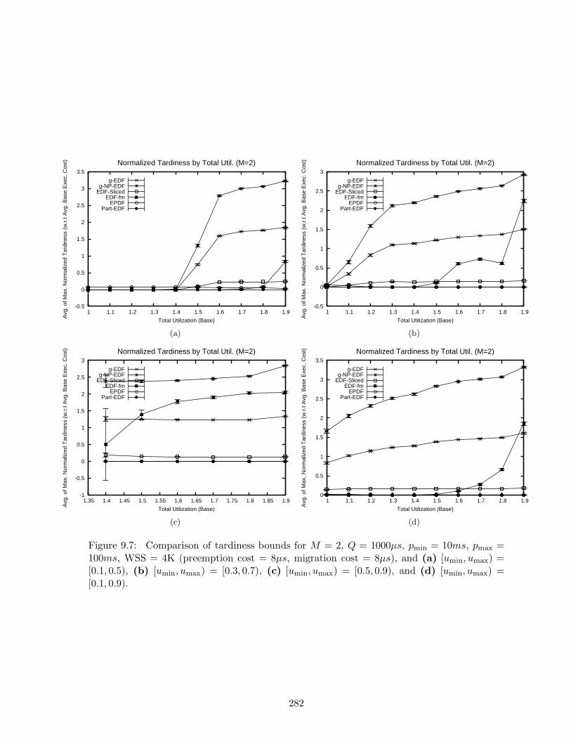
-0.5

0

0.5

1

1.5

2

2.5

3

3.5

1 1.1 1.2 1.3 1.4 1.5 1.6 1.7 1.8 1.9

Avg

. of M

ax. N

orm

aliz

ed T

ardi

ness

(w

.r.t

Avg

. Bas

e E

xec.

Cos

t)


Normalized Tardiness by Total Util. (M=2)

g-EDFg-NP-EDF

EDF-SlicedEDF-fm

EPDFPart-EDF

(a)

-0.5

0

0.5

1

1.5

2

2.5

3

1 1.1 1.2 1.3 1.4 1.5 1.6 1.7 1.8 1.9

Avg

. of M

ax. N

orm

aliz

ed T

ardi

ness

(w

.r.t

Avg

. Bas

e E

xec.

Cos

t)



g-EDFg-NP-EDF

EDF-SlicedEDF-fm

EPDFPart-EDF

(b)

-1

-0.5

0

0.5

1

1.5

2

2.5

3

1.35 1.4 1.45 1.5 1.55 1.6 1.65 1.7 1.75 1.8 1.85 1.9

Avg

. of M

ax. N

orm

aliz

ed T

ardi

ness

(w

.r.t

Avg

. Bas

e E

xec.

Cos

t)



g-EDFg-NP-EDF

EDF-SlicedEDF-fm

EPDFPart-EDF

(c)

0

0.5

1

1.5

2

2.5

3

3.5

1 1.1 1.2 1.3 1.4 1.5 1.6 1.7 1.8 1.9

Avg

. of M

ax. N

orm

aliz

ed T

ardi

ness

(w

.r.t

Avg

. Bas

e E

xec.

Cos

t)



g-EDFg-NP-EDF

EDF-SlicedEDF-fm

EPDFPart-EDF

(d)

Figure 9.7: Comparison of tardiness bounds for M = 2, Q = 1000µs, pmin = 10ms, pmax =100ms, WSS = 4K (preemption cost = 8µs, migration cost = 8µs), and (a) [umin, umax) =[0.1, 0.5), (b) [umin, umax) = [0.3, 0.7), (c) [umin, umax) = [0.5, 0.9), and (d) [umin, umax) =[0.1, 0.9).

282

0

2000

4000

6000

8000

10000

1 1.1 1.2 1.3 1.4 1.5 1.6 1.7 1.8 1.9

Num

ber

of S

ched

ulab

le T

ask

Set

s




g-NP-EDFEDF-Sliced

EDF-fmEPDF

P-EDF

(a)

0

2000

4000

6000

8000

10000

1 1.1 1.2 1.3 1.4 1.5 1.6 1.7 1.8 1.9

Num

ber

of S

ched

ulab

le T

ask

Set

s




g-NP-EDFEDF-Sliced

EDF-fmEPDF

P-EDF

(b)

0

2000

4000

6000

8000

10000

1.35 1.4 1.45 1.5 1.55 1.6 1.65 1.7 1.75 1.8 1.85 1.9

Num

ber

of S

ched

ulab

le T

ask

Set

s




g-NP-EDFEDF-Sliced

EDF-fmEPDF

P-EDF

(c)

0

2000

4000

6000

8000

10000

1 1.1 1.2 1.3 1.4 1.5 1.6 1.7 1.8 1.9

Num

ber

of S

ched

ulab

le T

ask

Set

s




g-NP-EDFEDF-Sliced

EDF-fmEPDF

P-EDF

(d)

Figure 9.8: Schedulability comparison for M = 2, Q = 1000µs, pmin = 10ms, pmax = 100ms,WSS = 64K (preemption cost = 58µs, migration cost = 64µs), and (a) [umin, umax) = [0.1, 0.5),(b) [umin, umax) = [0.3, 0.7), (c) [umin, umax) = [0.5, 0.9), and (d) [umin, umax) = [0.1, 0.9).

283

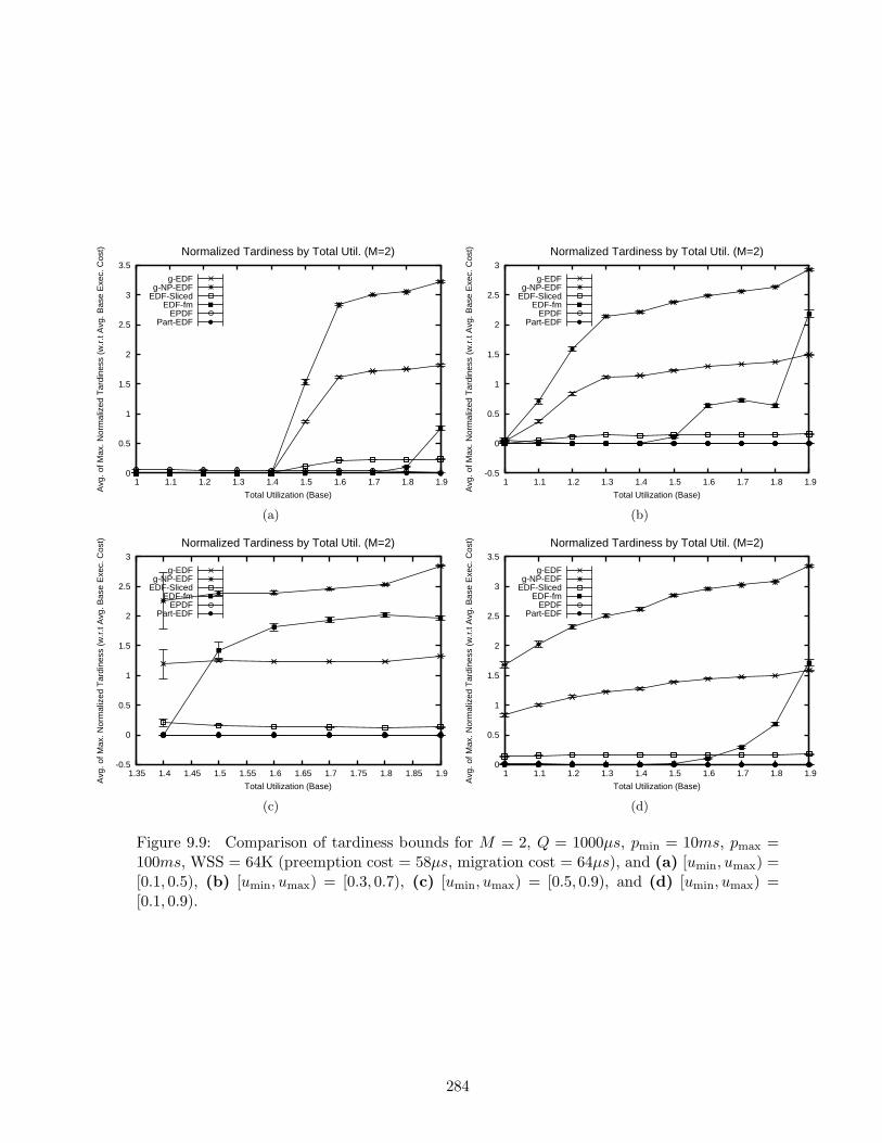
0

0.5

1

1.5

2

2.5

3

3.5

1 1.1 1.2 1.3 1.4 1.5 1.6 1.7 1.8 1.9

Avg

. of M

ax. N

orm

aliz

ed T

ardi

ness

(w

.r.t

Avg

. Bas

e E

xec.

Cos

t)



g-EDFg-NP-EDF

EDF-SlicedEDF-fm

EPDFPart-EDF

(a)

-0.5

0

0.5

1

1.5

2

2.5

3

1 1.1 1.2 1.3 1.4 1.5 1.6 1.7 1.8 1.9

Avg

. of M

ax. N

orm

aliz

ed T

ardi

ness

(w

.r.t

Avg

. Bas

e E

xec.

Cos

t)



g-EDFg-NP-EDF

EDF-SlicedEDF-fm

EPDFPart-EDF

(b)

-0.5

0

0.5

1

1.5

2

2.5

3

1.35 1.4 1.45 1.5 1.55 1.6 1.65 1.7 1.75 1.8 1.85 1.9

Avg

. of M

ax. N

orm

aliz

ed T

ardi

ness

(w

.r.t

Avg

. Bas

e E

xec.

Cos

t)



g-EDFg-NP-EDF

EDF-SlicedEDF-fm

EPDFPart-EDF

(c)

0

0.5

1

1.5

2

2.5

3

3.5

1 1.1 1.2 1.3 1.4 1.5 1.6 1.7 1.8 1.9

Avg

. of M

ax. N

orm

aliz

ed T

ardi

ness

(w

.r.t

Avg

. Bas

e E

xec.

Cos

t)



g-EDFg-NP-EDF

EDF-SlicedEDF-fm

EPDFPart-EDF

(d)


284

0

2000

4000

6000

8000

10000

1 1.1 1.2 1.3 1.4 1.5 1.6 1.7 1.8 1.9

Num

ber

of S

ched

ulab

le T

ask

Set

s




g-NP-EDFEDF-Sliced

EDF-fmEPDF

P-EDF

(a)

0

2000

4000

6000

8000

10000

1 1.1 1.2 1.3 1.4 1.5 1.6 1.7 1.8 1.9

Num

ber

of S

ched

ulab

le T

ask

Set

s




g-NP-EDFEDF-Sliced

EDF-fmEPDF

P-EDF

(b)

0

2000

4000

6000

8000

10000

1.35 1.4 1.45 1.5 1.55 1.6 1.65 1.7 1.75 1.8 1.85 1.9

Num

ber

of S

ched

ulab

le T

ask

Set

s




g-NP-EDFEDF-Sliced

EDF-fmEPDF

P-EDF

(c)

0

2000

4000

6000

8000

10000

1 1.1 1.2 1.3 1.4 1.5 1.6 1.7 1.8 1.9

Num

ber

of S

ched

ulab

le T

ask

Set

s




g-NP-EDFEDF-Sliced

EDF-fmEPDF

P-EDF

(d)

Figure 9.10: Schedulability comparison for M = 2, Q = 1000µs, pmin = 10ms, pmax = 100ms,WSS = 128K (preemption cost = 116µs, migration cost = 136µs), and (a) [umin, umax) =[0.1, 0.5), (b) [umin, umax) = [0.3, 0.7), (c) [umin, umax) = [0.5, 0.9), and (d) [umin, umax) =[0.1, 0.9).

285

-0.5

0

0.5

1

1.5

2

2.5

3

3.5

1 1.1 1.2 1.3 1.4 1.5 1.6 1.7 1.8 1.9

Avg

. of M

ax. N

orm

aliz

ed T

ardi

ness

(w

.r.t

Avg

. Bas

e E

xec.

Cos

t)



g-EDFg-NP-EDF

EDF-SlicedEDF-fm

EPDFPart-EDF

(a)

-0.5

0

0.5

1

1.5

2

2.5

3

1 1.1 1.2 1.3 1.4 1.5 1.6 1.7 1.8 1.9

Avg

. of M

ax. N

orm

aliz

ed T

ardi

ness

(w

.r.t

Avg

. Bas

e E

xec.

Cos

t)



g-EDFg-NP-EDF

EDF-SlicedEDF-fm

EPDFPart-EDF

(b)

-1

-0.5

0

0.5

1

1.5

2

2.5

3

1.35 1.4 1.45 1.5 1.55 1.6 1.65 1.7 1.75 1.8 1.85 1.9

Avg

. of M

ax. N

orm

aliz

ed T

ardi

ness

(w

.r.t

Avg

. Bas

e E

xec.

Cos

t)



g-EDFg-NP-EDF

EDF-SlicedEDF-fm

EPDFPart-EDF

(c)

0

0.5

1

1.5

2

2.5

3

3.5

1 1.1 1.2 1.3 1.4 1.5 1.6 1.7 1.8 1.9

Avg

. of M

ax. N

orm

aliz

ed T

ardi

ness

(w

.r.t

Avg

. Bas

e E

xec.

Cos

t)



g-EDFg-NP-EDF

EDF-SlicedEDF-fm

EPDFPart-EDF

(d)

Figure 9.11: Comparison of tardiness bounds for M = 2, Q = 1000µs, pmin = 10ms,pmax = 100ms, WSS = 128K (preemption cost = 116µs, migration cost = 136µs), and (a)[umin, umax) = [0.1, 0.5), (b) [umin, umax) = [0.3, 0.7), (c) [umin, umax) = [0.5, 0.9), and (d)[umin, umax) = [0.1, 0.9).

286

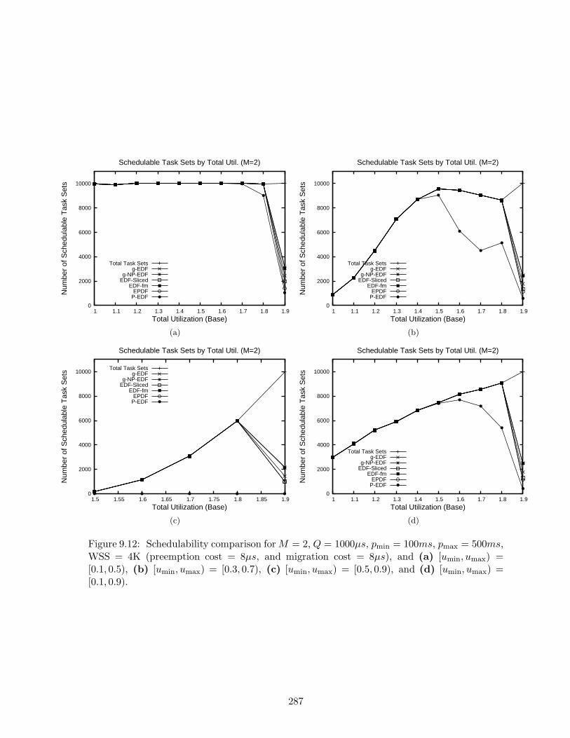
0

2000

4000

6000

8000

10000

1 1.1 1.2 1.3 1.4 1.5 1.6 1.7 1.8 1.9

Num

ber

of S

ched

ulab

le T

ask

Set

s




g-NP-EDFEDF-Sliced

EDF-fmEPDF

P-EDF

(a)

0

2000

4000

6000

8000

10000

1 1.1 1.2 1.3 1.4 1.5 1.6 1.7 1.8 1.9

Num

ber

of S

ched

ulab

le T

ask

Set

s




g-NP-EDFEDF-Sliced

EDF-fmEPDF

P-EDF

(b)

0

2000

4000

6000

8000

10000

1.5 1.55 1.6 1.65 1.7 1.75 1.8 1.85 1.9

Num

ber

of S

ched

ulab

le T

ask

Set

s




g-NP-EDFEDF-Sliced

EDF-fmEPDF

P-EDF

(c)

0

2000

4000

6000

8000

10000

1 1.1 1.2 1.3 1.4 1.5 1.6 1.7 1.8 1.9

Num

ber

of S

ched

ulab

le T

ask

Set

s




g-NP-EDFEDF-Sliced

EDF-fmEPDF

P-EDF

(d)


287

0

0.5

1

1.5

2

2.5

3

1 1.1 1.2 1.3 1.4 1.5 1.6 1.7 1.8 1.9

Avg

. of M

ax. N

orm

aliz

ed T

ardi

ness

(w

.r.t

Avg

. Bas

e E

xec.

Cos

t)



g-EDFg-NP-EDF

EDF-SlicedEDF-fm

EPDFPart-EDF

(a)

0

0.5

1

1.5

2

2.5

3

1 1.1 1.2 1.3 1.4 1.5 1.6 1.7 1.8 1.9

Avg

. of M

ax. N

orm

aliz

ed T

ardi

ness

(w

.r.t

Avg

. Bas

e E

xec.

Cos

t)



g-EDFg-NP-EDF

EDF-SlicedEDF-fm

EPDFPart-EDF

(b)

0

0.5

1

1.5

2

2.5

3

1.5 1.55 1.6 1.65 1.7 1.75 1.8 1.85 1.9

Avg

. of M

ax. N

orm

aliz

ed T

ardi

ness

(w

.r.t

Avg

. Bas

e E

xec.

Cos

t)



g-EDFg-NP-EDF

EDF-SlicedEDF-fm

EPDFPart-EDF

(c)

0

0.5

1

1.5

2

2.5

3

3.5

1 1.1 1.2 1.3 1.4 1.5 1.6 1.7 1.8 1.9

Avg

. of M

ax. N

orm

aliz

ed T

ardi

ness

(w

.r.t

Avg

. Bas

e E

xec.

Cos

t)



g-EDFg-NP-EDF

EDF-SlicedEDF-fm

EPDFPart-EDF

(d)


288

0

2000

4000

6000

8000

10000

1 1.1 1.2 1.3 1.4 1.5 1.6 1.7 1.8 1.9

Num

ber

of S

ched

ulab

le T

ask

Set

s




g-NP-EDFEDF-Sliced

EDF-fmEPDF

P-EDF

(a)

0

2000

4000

6000

8000

10000

1 1.1 1.2 1.3 1.4 1.5 1.6 1.7 1.8 1.9

Num

ber

of S

ched

ulab

le T

ask

Set

s




g-NP-EDFEDF-Sliced

EDF-fmEPDF

P-EDF

(b)

0

2000

4000

6000

8000

10000

1.5 1.55 1.6 1.65 1.7 1.75 1.8 1.85 1.9

Num

ber

of S

ched

ulab

le T

ask

Set

s




g-NP-EDFEDF-Sliced

EDF-fmEPDF

P-EDF

(c)

0

2000

4000

6000

8000

10000

1 1.1 1.2 1.3 1.4 1.5 1.6 1.7 1.8 1.9

Num

ber

of S

ched

ulab

le T

ask

Set

s




g-NP-EDFEDF-Sliced

EDF-fmEPDF

P-EDF

(d)

Figure 9.14: Schedulability comparison for M = 2, Q = 1000µs, pmin = 100ms, pmax = 500ms,WSS = 64K (preemption cost = 58µs, migration cost = 64µs), and (a) [umin, umax) = [0.1, 0.5),(b) [umin, umax) = [0.3, 0.7), (c) [umin, umax) = [0.5, 0.9), and (d) [umin, umax) = [0.1, 0.9).

289

0

0.5

1

1.5

2

2.5

3

1 1.1 1.2 1.3 1.4 1.5 1.6 1.7 1.8 1.9

Avg

. of M

ax. N

orm

aliz

ed T

ardi

ness

(w

.r.t

Avg

. Bas

e E

xec.

Cos

t)



g-EDFg-NP-EDF

EDF-SlicedEDF-fm

EPDFPart-EDF

(a)

0

0.5

1

1.5

2

2.5

3

1 1.1 1.2 1.3 1.4 1.5 1.6 1.7 1.8 1.9

Avg

. of M

ax. N

orm

aliz

ed T

ardi

ness

(w

.r.t

Avg

. Bas

e E

xec.

Cos

t)



g-EDFg-NP-EDF

EDF-SlicedEDF-fm

EPDFPart-EDF

(b)

0

0.5

1

1.5

2

2.5

3

1.5 1.55 1.6 1.65 1.7 1.75 1.8 1.85 1.9

Avg

. of M

ax. N

orm

aliz

ed T

ardi

ness

(w

.r.t

Avg

. Bas

e E

xec.

Cos

t)



g-EDFg-NP-EDF

EDF-SlicedEDF-fm

EPDFPart-EDF

(c)

0

0.5

1

1.5

2

2.5

3

3.5

1 1.1 1.2 1.3 1.4 1.5 1.6 1.7 1.8 1.9

Avg

. of M

ax. N

orm

aliz

ed T

ardi

ness

(w

.r.t

Avg

. Bas

e E

xec.

Cos

t)



g-EDFg-NP-EDF

EDF-SlicedEDF-fm

EPDFPart-EDF

(d)


290

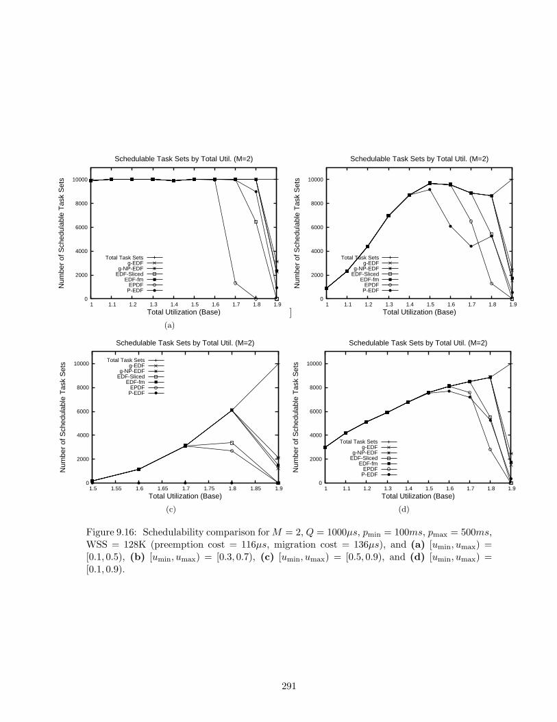
0

2000

4000

6000

8000

10000

1 1.1 1.2 1.3 1.4 1.5 1.6 1.7 1.8 1.9

Num

ber

of S

ched

ulab

le T

ask

Set

s




g-NP-EDFEDF-Sliced

EDF-fmEPDF

P-EDF

(a)

]

0

2000

4000

6000

8000

10000

1 1.1 1.2 1.3 1.4 1.5 1.6 1.7 1.8 1.9N

umbe

r of

Sch

edul

able

Tas

k S

ets




g-NP-EDFEDF-Sliced

EDF-fmEPDF

P-EDF

0

2000

4000

6000

8000

10000

1.5 1.55 1.6 1.65 1.7 1.75 1.8 1.85 1.9

Num

ber

of S

ched

ulab

le T

ask

Set

s




g-NP-EDFEDF-Sliced

EDF-fmEPDF

P-EDF

(c)

0

2000

4000

6000

8000

10000

1 1.1 1.2 1.3 1.4 1.5 1.6 1.7 1.8 1.9

Num

ber

of S

ched

ulab

le T

ask

Set

s




g-NP-EDFEDF-Sliced

EDF-fmEPDF

P-EDF

(d)


291

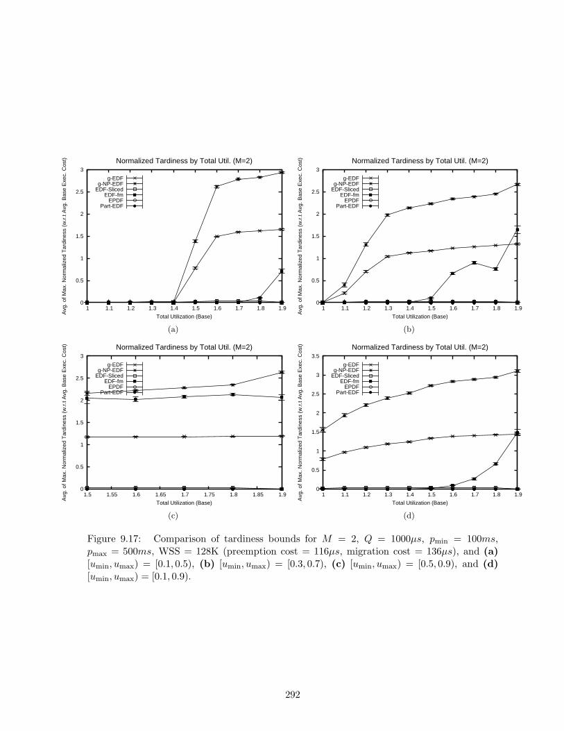
0

0.5

1

1.5

2

2.5

3

1 1.1 1.2 1.3 1.4 1.5 1.6 1.7 1.8 1.9

Avg

. of M

ax. N

orm

aliz

ed T

ardi

ness

(w

.r.t

Avg

. Bas

e E

xec.

Cos

t)



g-EDFg-NP-EDF

EDF-SlicedEDF-fm

EPDFPart-EDF

(a)

0

0.5

1

1.5

2

2.5

3

1 1.1 1.2 1.3 1.4 1.5 1.6 1.7 1.8 1.9

Avg

. of M

ax. N

orm

aliz

ed T

ardi

ness

(w

.r.t

Avg

. Bas

e E

xec.

Cos

t)



g-EDFg-NP-EDF

EDF-SlicedEDF-fm

EPDFPart-EDF

(b)

0

0.5

1

1.5

2

2.5

3

1.5 1.55 1.6 1.65 1.7 1.75 1.8 1.85 1.9

Avg

. of M

ax. N

orm

aliz

ed T

ardi

ness

(w

.r.t

Avg

. Bas

e E

xec.

Cos

t)



g-EDFg-NP-EDF

EDF-SlicedEDF-fm

EPDFPart-EDF

(c)

0

0.5

1

1.5

2

2.5

3

3.5

1 1.1 1.2 1.3 1.4 1.5 1.6 1.7 1.8 1.9

Avg

. of M

ax. N

orm

aliz

ed T

ardi

ness

(w

.r.t

Avg

. Bas

e E

xec.

Cos

t)



g-EDFg-NP-EDF

EDF-SlicedEDF-fm

EPDFPart-EDF

(d)


292

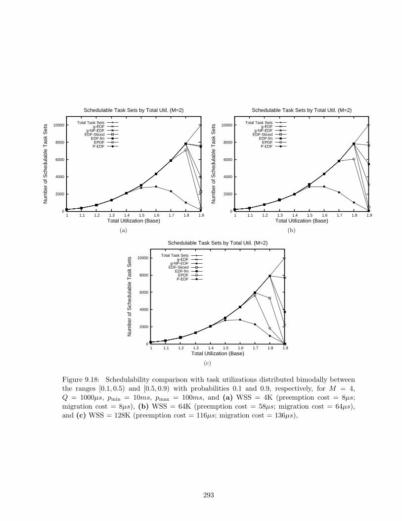
0

2000

4000

6000

8000

10000

1 1.1 1.2 1.3 1.4 1.5 1.6 1.7 1.8 1.9

Num

ber

of S

ched

ulab

le T

ask

Set

s




g-NP-EDFEDF-Sliced

EDF-fmEPDF

P-EDF

(a)

0

2000

4000

6000

8000

10000

1 1.1 1.2 1.3 1.4 1.5 1.6 1.7 1.8 1.9N

umbe

r of

Sch

edul

able

Tas

k S

ets




g-NP-EDFEDF-Sliced

EDF-fmEPDF

P-EDF

(b)

0

2000

4000

6000

8000

10000

1 1.1 1.2 1.3 1.4 1.5 1.6 1.7 1.8 1.9

Num

ber

of S

ched

ulab

le T

ask

Set

s




g-NP-EDFEDF-Sliced

EDF-fmEPDF

P-EDF

(c)

Figure 9.18: Schedulability comparison with task utilizations distributed bimodally betweenthe ranges [0.1, 0.5) and [0.5, 0.9) with probabilities 0.1 and 0.9, respectively, for M = 4,Q = 1000µs, pmin = 10ms, pmax = 100ms, and (a) WSS = 4K (preemption cost = 8µs;migration cost = 8µs), (b) WSS = 64K (preemption cost = 58µs; migration cost = 64µs),and (c) WSS = 128K (preemption cost = 116µs; migration cost = 136µs),

293

Impact of preemption and migration costs. To study the impact of preemption and

migration costs on the various algorithms, we will consider Figures 9.19–9.24, which plot the

results for the three preemption and migration costs considered when M = 4. Comparing

corresponding insets of Figures 9.19, 9.21, and 9.23, which are for WSSs of 4K (preemption

cost = 16µs, migration cost = 16µs), 64K (preemption cost = 116µs, migration cost = 128µs),

and 128K (preemption cost = 232µs, migration cost = 272µs), respectively, it is evident that

EPDF and EDF-sliced are impacted the most by increasing preemption and migration costs.

This is in line with the fact that under EPDF and EDF-sliced, each job can be charged with

the cost of multiple migrations, whereas under the remaining algorithms, each job is charged

with exactly one migration or preemption cost. Considering the remaining algorithms, g-

NP-EDF is unaffected as it suffers no preemptions or migrations, and g-EDF is impacted by

approximately equal extents at all per-task utilization ranges, whereas the impact to p-EDF

and EDF-fm is higher at lower per-task utilizations. This trend observed with p-EDF and EDF-

fm is due to the fact that under these algorithms, as task utilizations increase, schedulability

is more adversely impacted by difficulties in partitioning tasks among processors than by

preemption overheads. Some other trends to observe are as follows. Though g-EDF is impacted

by increasing preemption and migration costs, its performance is comparable to that of g-NP-

EDF for all WSSs even when total utilization is as high as 90%. The schedulability of g-EDF

is higher than that of p-EDF for all WSSs considered, and that of EPDF and EDF-sliced are

higher than that of p-EDF when tasks are predominantly heavy, again, for all WSSs).

Comparing the tardiness bounds reported in Figures 9.20, 9.22, and 9.24, trends among

the insets of any figure are as described in the context of the impact of task utilization costs.

Not much difference is exhibited by corresponding insets of figures associated with different

preemption and migration costs.

Impact of M . Barring a few exceptions, varying M while keeping other parameters fixed

(or, in the case of preemption and migration costs normalized with respect to M), worsens

schedulability equally for all the algorithms. For example, compare corresponding insets of

Figures 9.6 and 9.19 or of Figures 9.8 and 9.21. This is due to the assumption that preemption

and migration costs increase linearly with increasing M . Therefore, the impact is higher

when higher normalized (base) preemption and migration costs are assumed. One significant

deviation from this general trend is that the loss incurred by EDF-fm is significantly higher

when moving from M = 2 to M = 4 when task utilizations are high. This is due to the

294

difficulties in task assignment with heavy tasks on more than two processors. In a somewhat

similar vein, EPDF and EDF-sliced take a heavy hit when moving from M = 4 to M = 8 for

periods in the range [10, 100) due to high migration costs. It can also be seen that tardiness

bounds guaranteed by the non-partitioned EDF algorithms increase with increasing M .

Impact of task periods. As discussed earlier, for algorithms other than EPDF and EDF-

sliced, most overheads, with the significant exception of the tick-scheduling overhead, charged

per unit of execution cost of a job, decrease with increasing base execution costs (and hence,

increasing task periods for a given task utilization). (The tick-scheduling overhead charged

per unit of job execution cost is independent of the total execution cost of a job.) Therefore,

for these algorithms, in general, the larger the job size, the lower the overheads. A rough

estimate of the improvement in schedulability, if any, as the range for periods is increased from

[10, 100) to [100, 500) for a given per-task utilization range can be discerned by comparing

corresponding insets of any two schedulability figures that differ only in the period parameter.

Since preemption and migration costs constitute the predominant overhead, gains are the

highest when migration costs are the highest. For example, compare Figures 9.23 and 9.29.

[pmin, pmax) is [10, 100) for the former and [100, 500) for the latter. Preemption and migration

costs are 232µs and 272µs, respectively, in both these figures. In inset (a) of the first figure,

the percentage of schedulable task sets for g-EDF is zero when base total utilization is 3.9,

whereas it is close to 20% in the second figure. Similar, though slightly lower, gains can be

observed for g-EDF in the other insets also. For p-EDF and EDF-fm, gains are noticeably

higher for lower per-task utilizations than for higher per-task utilizations. This trend again, as

explained in other contexts, is due to the fact that difficulties in partitioning more adversely

impact schedulability than the other overheads as task utilizations increase.

Considering the remaining three algorithms, surprisingly, schedulability improves signifi-

cantly for EPDF, which can be attributed to a decrease in the rounding overhead with increasing

execution cost (regardless of the period). Though schedulability seems to be decreasing for

EDF-sliced and g-NP-EDF, this trend is simply an artifact of the bin sizes used on the x-axis.

In our schedulability plots, each point along the x-axis spans a utilization range that is 0.1

units wide; for instance, point 3.0 corresponds to the range [3.0, 3.1). With larger periods, the

distribution of total utilizations of task sets is skewed toward the higher end of the range, i.e.,

within a range, more task sets are generated with total base utilizations in the higher end, and

hence, more are found to be not schedulable. For instance, if our point of interest along the

295

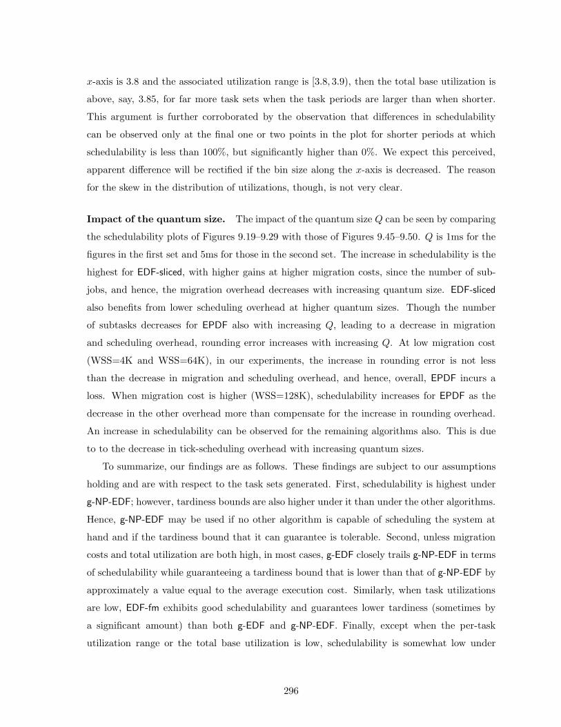
x-axis is 3.8 and the associated utilization range is [3.8, 3.9), then the total base utilization is

above, say, 3.85, for far more task sets when the task periods are larger than when shorter.

This argument is further corroborated by the observation that differences in schedulability

can be observed only at the final one or two points in the plot for shorter periods at which

schedulability is less than 100%, but significantly higher than 0%. We expect this perceived,

apparent difference will be rectified if the bin size along the x-axis is decreased. The reason

for the skew in the distribution of utilizations, though, is not very clear.

Impact of the quantum size. The impact of the quantum size Q can be seen by comparing

the schedulability plots of Figures 9.19–9.29 with those of Figures 9.45–9.50. Q is 1ms for the

figures in the first set and 5ms for those in the second set. The increase in schedulability is the

highest for EDF-sliced, with higher gains at higher migration costs, since the number of sub-

jobs, and hence, the migration overhead decreases with increasing quantum size. EDF-sliced

also benefits from lower scheduling overhead at higher quantum sizes. Though the number

of subtasks decreases for EPDF also with increasing Q, leading to a decrease in migration

and scheduling overhead, rounding error increases with increasing Q. At low migration cost

(WSS=4K and WSS=64K), in our experiments, the increase in rounding error is not less

than the decrease in migration and scheduling overhead, and hence, overall, EPDF incurs a

loss. When migration cost is higher (WSS=128K), schedulability increases for EPDF as the

decrease in the other overhead more than compensate for the increase in rounding overhead.

An increase in schedulability can be observed for the remaining algorithms also. This is due

to to the decrease in tick-scheduling overhead with increasing quantum sizes.

To summarize, our findings are as follows. These findings are subject to our assumptions

holding and are with respect to the task sets generated. First, schedulability is highest under

g-NP-EDF; however, tardiness bounds are also higher under it than under the other algorithms.

Hence, g-NP-EDF may be used if no other algorithm is capable of scheduling the system at

hand and if the tardiness bound that it can guarantee is tolerable. Second, unless migration

costs and total utilization are both high, in most cases, g-EDF closely trails g-NP-EDF in terms

of schedulability while guaranteeing a tardiness bound that is lower than that of g-NP-EDF by

approximately a value equal to the average execution cost. Similarly, when task utilizations

are low, EDF-fm exhibits good schedulability and guarantees lower tardiness (sometimes by

a significant amount) than both g-EDF and g-NP-EDF. Finally, except when the per-task

utilization range or the total base utilization is low, schedulability is somewhat low under

296

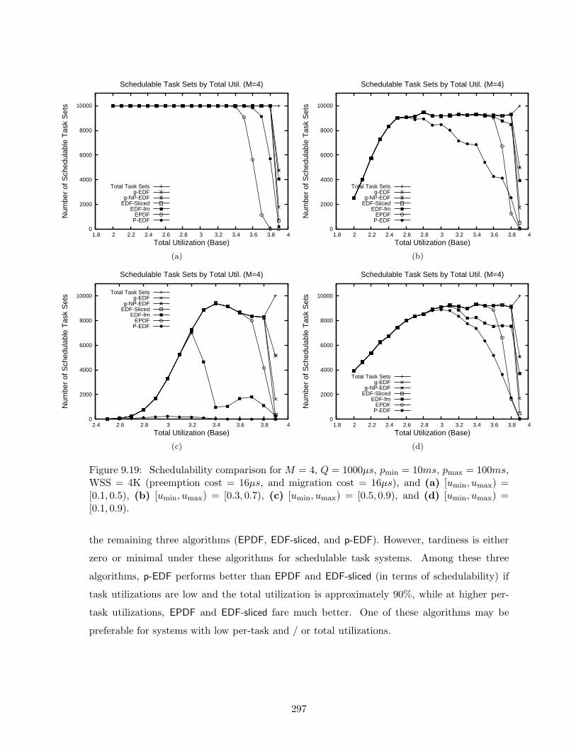
0

2000

4000

6000

8000

10000

1.8 2 2.2 2.4 2.6 2.8 3 3.2 3.4 3.6 3.8 4

Num

ber

of S

ched

ulab

le T

ask

Set

s




g-NP-EDFEDF-Sliced

EDF-fmEPDF

P-EDF

(a)

0

2000

4000

6000

8000

10000

1.8 2 2.2 2.4 2.6 2.8 3 3.2 3.4 3.6 3.8 4

Num

ber

of S

ched

ulab

le T

ask

Set

s




g-NP-EDFEDF-Sliced

EDF-fmEPDF

P-EDF

(b)

0

2000

4000

6000

8000

10000

2.4 2.6 2.8 3 3.2 3.4 3.6 3.8 4

Num

ber

of S

ched

ulab

le T

ask

Set

s




g-NP-EDFEDF-Sliced

EDF-fmEPDF

P-EDF

(c)

0

2000

4000

6000

8000

10000

1.8 2 2.2 2.4 2.6 2.8 3 3.2 3.4 3.6 3.8 4

Num

ber

of S

ched

ulab

le T

ask

Set

s




g-NP-EDFEDF-Sliced

EDF-fmEPDF

P-EDF

(d)


the remaining three algorithms (EPDF, EDF-sliced, and p-EDF). However, tardiness is either

zero or minimal under these algorithms for schedulable task systems. Among these three

algorithms, p-EDF performs better than EPDF and EDF-sliced (in terms of schedulability) if

task utilizations are low and the total utilization is approximately 90%, while at higher per-

task utilizations, EPDF and EDF-sliced fare much better. One of these algorithms may be

preferable for systems with low per-task and / or total utilizations.

297

0

0.5

1

1.5

2

2.5

3

3.5

4

1.8 2 2.2 2.4 2.6 2.8 3 3.2 3.4 3.6 3.8 4

Avg

. of M

ax. N

orm

aliz

ed T

ardi

ness

(w

.r.t

Avg

. Bas

e E

xec.

Cos

t)



g-EDFg-NP-EDF

EDF-SlicedEDF-fm

EPDFPart-EDF

(a)

0

1

2

3

4

5

6

1.8 2 2.2 2.4 2.6 2.8 3 3.2 3.4 3.6 3.8 4

Avg

. of M

ax. N

orm

aliz

ed T

ardi

ness

(w

.r.t

Avg

. Bas

e E

xec.

Cos

t)



g-EDFg-NP-EDF

EDF-SlicedEDF-fm

EPDFPart-EDF

(b)

0

2

4

6

8

10

12

2.4 2.6 2.8 3 3.2 3.4 3.6 3.8 4

Avg

. of M

ax. N

orm

aliz

ed T

ardi

ness

(w

.r.t

Avg

. Bas

e E

xec.

Cos

t)



g-EDFg-NP-EDF

EDF-SlicedEDF-fm

EPDFPart-EDF

(c)

0

0.5

1

1.5

2

2.5

3

3.5

4

4.5

1.8 2 2.2 2.4 2.6 2.8 3 3.2 3.4 3.6 3.8 4

Avg

. of M

ax. N

orm

aliz

ed T

ardi

ness

(w

.r.t

Avg

. Bas

e E

xec.

Cos

t)



g-EDFg-NP-EDF

EDF-SlicedEDF-fm

EPDFPart-EDF

(d)


298

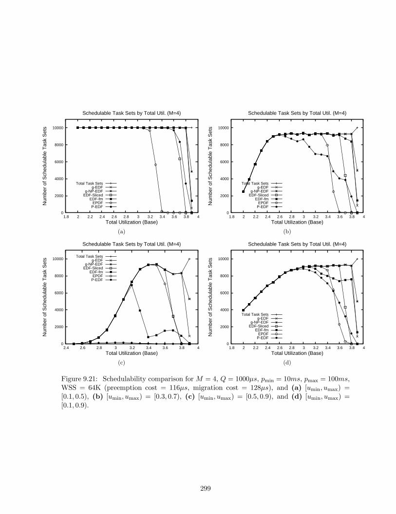
0

2000

4000

6000

8000

10000

1.8 2 2.2 2.4 2.6 2.8 3 3.2 3.4 3.6 3.8 4

Num

ber

of S

ched

ulab

le T

ask

Set

s




g-NP-EDFEDF-Sliced

EDF-fmEPDF

P-EDF

(a)

0

2000

4000

6000

8000

10000

1.8 2 2.2 2.4 2.6 2.8 3 3.2 3.4 3.6 3.8 4

Num

ber

of S

ched

ulab

le T

ask

Set

s




g-NP-EDFEDF-Sliced

EDF-fmEPDF

P-EDF

(b)

0

2000

4000

6000

8000

10000

2.4 2.6 2.8 3 3.2 3.4 3.6 3.8 4

Num

ber

of S

ched

ulab

le T

ask

Set

s




g-NP-EDFEDF-Sliced

EDF-fmEPDF

P-EDF

(c)

0

2000

4000

6000

8000

10000

1.8 2 2.2 2.4 2.6 2.8 3 3.2 3.4 3.6 3.8 4

Num

ber

of S

ched

ulab

le T

ask

Set

s




g-NP-EDFEDF-Sliced

EDF-fmEPDF

P-EDF

(d)


299

0

0.5

1

1.5

2

2.5

3

3.5

4

1.8 2 2.2 2.4 2.6 2.8 3 3.2 3.4 3.6 3.8 4

Avg

. of M

ax. N

orm

aliz

ed T

ardi

ness

(w

.r.t

Avg

. Bas

e E

xec.

Cos

t)



g-EDFg-NP-EDF

EDF-SlicedEDF-fm

EPDFPart-EDF

(a)

0

0.5

1

1.5

2

2.5

3

3.5

4

4.5

5

1.8 2 2.2 2.4 2.6 2.8 3 3.2 3.4 3.6 3.8 4

Avg

. of M

ax. N

orm

aliz

ed T

ardi

ness

(w

.r.t

Avg

. Bas

e E

xec.

Cos

t)



g-EDFg-NP-EDF

EDF-SlicedEDF-fm

EPDFPart-EDF

(b)

0

2

4

6

8

10

12

2.4 2.6 2.8 3 3.2 3.4 3.6 3.8 4

Avg

. of M

ax. N

orm

aliz

ed T

ardi

ness

(w

.r.t

Avg

. Bas

e E

xec.

Cos

t)



g-EDFg-NP-EDF

EDF-SlicedEDF-fm

EPDFPart-EDF

(c)

0

0.5

1

1.5

2

2.5

3

3.5

4

4.5

1.8 2 2.2 2.4 2.6 2.8 3 3.2 3.4 3.6 3.8 4

Avg

. of M

ax. N

orm

aliz

ed T

ardi

ness

(w

.r.t

Avg

. Bas

e E

xec.

Cos

t)



g-EDFg-NP-EDF

EDF-SlicedEDF-fm

EPDFPart-EDF

(d)


300

0

2000

4000

6000

8000

10000

1.8 2 2.2 2.4 2.6 2.8 3 3.2 3.4 3.6 3.8 4

Num

ber

of S

ched

ulab

le T

ask

Set

s




g-NP-EDFEDF-Sliced

EDF-fmEPDF

P-EDF

(a)

0

2000

4000

6000

8000

10000

1.8 2 2.2 2.4 2.6 2.8 3 3.2 3.4 3.6 3.8 4

Num

ber

of S

ched

ulab

le T

ask

Set

s




g-NP-EDFEDF-Sliced

EDF-fmEPDF

P-EDF

(b)

0

2000

4000

6000

8000

10000

2.2 2.4 2.6 2.8 3 3.2 3.4 3.6 3.8 4

Num

ber

of S

ched

ulab

le T

ask

Set

s




g-NP-EDFEDF-Sliced

EDF-fmEPDF

P-EDF

(c)

0

2000

4000

6000

8000

10000

1.8 2 2.2 2.4 2.6 2.8 3 3.2 3.4 3.6 3.8 4

Num

ber

of S

ched

ulab

le T

ask

Set

s




g-NP-EDFEDF-Sliced

EDF-fmEPDF

P-EDF

(d)


301

0

0.5

1

1.5

2

2.5

3

3.5

4

1.8 2 2.2 2.4 2.6 2.8 3 3.2 3.4 3.6 3.8 4

Avg

. of M

ax. N

orm

aliz

ed T

ardi

ness

(w

.r.t

Avg

. Bas

e E

xec.

Cos

t)



g-EDFg-NP-EDF

EDF-SlicedEDF-fm

EPDFPart-EDF

(a)

0

0.5

1

1.5

2

2.5

3

3.5

4

4.5

5

1.8 2 2.2 2.4 2.6 2.8 3 3.2 3.4 3.6 3.8 4A

vg. o

f Max

. Nor

mal

ized

Tar

dine

ss (

w.r

.t A

vg. B

ase

Exe

c. C

ost)



g-EDFg-NP-EDF

EDF-SlicedEDF-fm

EPDFPart-EDF

(b)

0

2

4

6

8

10

12

14

2.2 2.4 2.6 2.8 3 3.2 3.4 3.6 3.8 4

Avg

. of M

ax. N

orm

aliz

ed T

ardi

ness

(w

.r.t

Avg

. Bas

e E

xec.

Cos

t)



g-EDFg-NP-EDF

EDF-SlicedEDF-fm

EPDFPart-EDF

(c)

0

0.5

1

1.5

2

2.5

3

3.5

4

4.5

1.8 2 2.2 2.4 2.6 2.8 3 3.2 3.4 3.6 3.8 4

Avg

. of M

ax. N

orm

aliz

ed T

ardi

ness

(w

.r.t

Avg

. Bas

e E

xec.

Cos

t)



g-EDFg-NP-EDF

EDF-SlicedEDF-fm

EPDFPart-EDF

(d)

Figure 9.24: Tardiness bounds results for M = 4, Q = 1000µs, pmin = 10ms, pmax = 100ms,WSS = 128K Comparison of tardiness bounds for M = 4, Q = 1000µs, pmin = 10ms,pmax = 100ms, WSS = 128K (preemption cost = 232µs, migration cost = 272µs), and (a)[umin, umax) = [0.1, 0.5), (b) [umin, umax) = [0.3, 0.7), (c) [umin, umax) = [0.5, 0.9), and (d)[umin, umax) = [0.1, 0.9).

302

0

2000

4000

6000

8000

10000

1.8 2 2.2 2.4 2.6 2.8 3 3.2 3.4 3.6 3.8 4

Num

ber

of S

ched

ulab

le T

ask

Set

s




g-NP-EDFEDF-Sliced

EDF-fmEPDF

P-EDF

(a)

0

2000

4000

6000

8000

10000

1.8 2 2.2 2.4 2.6 2.8 3 3.2 3.4 3.6 3.8 4

Num

ber

of S

ched

ulab

le T

ask

Set

s




g-NP-EDFEDF-Sliced

EDF-fmEPDF

P-EDF

(b)

0

2000

4000

6000

8000

10000

2.4 2.6 2.8 3 3.2 3.4 3.6 3.8 4

Num

ber

of S

ched

ulab

le T

ask

Set

s




g-NP-EDFEDF-Sliced

EDF-fmEPDF

P-EDF

(c)

0

2000

4000

6000

8000

10000

1.8 2 2.2 2.4 2.6 2.8 3 3.2 3.4 3.6 3.8 4

Num

ber

of S

ched

ulab

le T

ask

Set

s




g-NP-EDFEDF-Sliced

EDF-fmEPDF

P-EDF

(d)


303

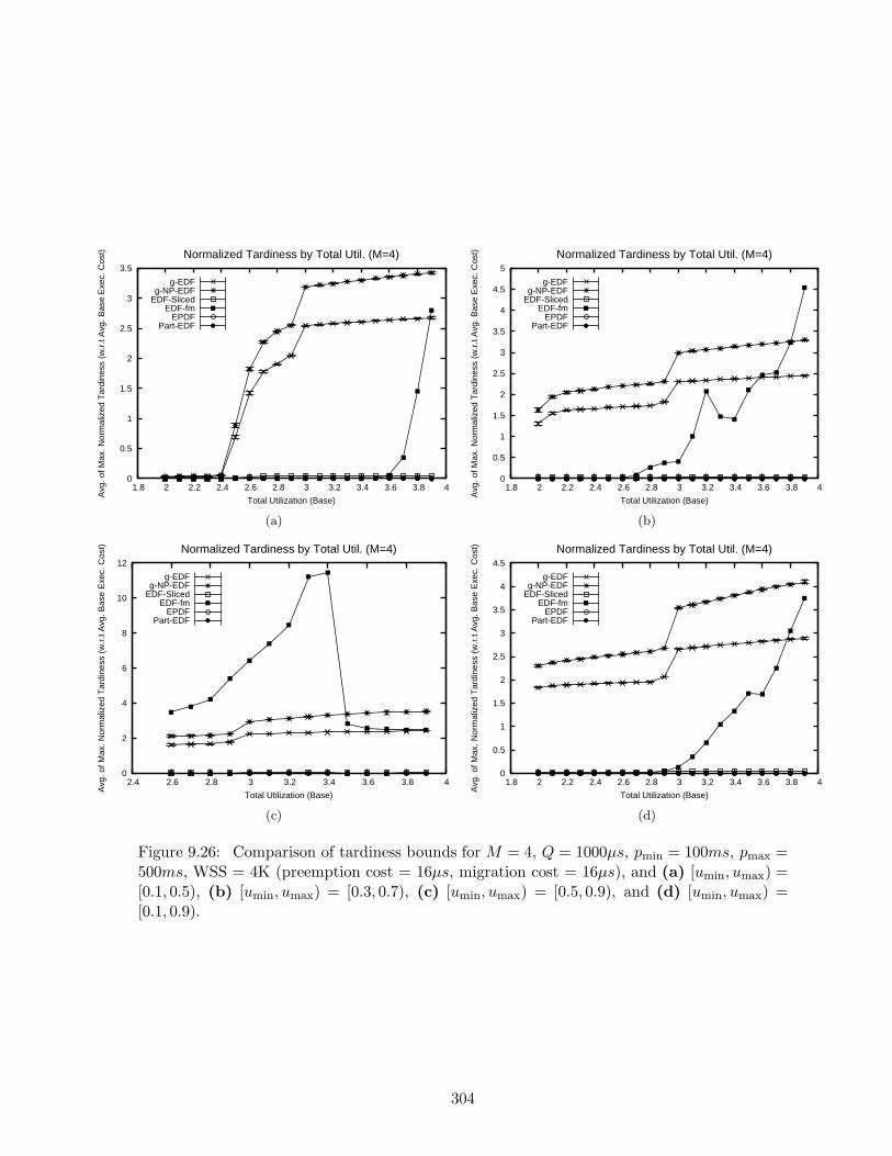
0

0.5

1

1.5

2

2.5

3

3.5

1.8 2 2.2 2.4 2.6 2.8 3 3.2 3.4 3.6 3.8 4

Avg

. of M

ax. N

orm

aliz

ed T

ardi

ness

(w

.r.t

Avg

. Bas

e E

xec.

Cos

t)



g-EDFg-NP-EDF

EDF-SlicedEDF-fm

EPDFPart-EDF

(a)

0

0.5

1

1.5

2

2.5

3

3.5

4

4.5

5

1.8 2 2.2 2.4 2.6 2.8 3 3.2 3.4 3.6 3.8 4

Avg

. of M

ax. N

orm

aliz

ed T

ardi

ness

(w

.r.t

Avg

. Bas

e E

xec.

Cos

t)



g-EDFg-NP-EDF

EDF-SlicedEDF-fm

EPDFPart-EDF

(b)

0

2

4

6

8

10

12

2.4 2.6 2.8 3 3.2 3.4 3.6 3.8 4

Avg

. of M

ax. N

orm

aliz

ed T

ardi

ness

(w

.r.t

Avg

. Bas

e E

xec.

Cos

t)



g-EDFg-NP-EDF

EDF-SlicedEDF-fm

EPDFPart-EDF

(c)

0

0.5

1

1.5

2

2.5

3

3.5

4

4.5

1.8 2 2.2 2.4 2.6 2.8 3 3.2 3.4 3.6 3.8 4

Avg

. of M

ax. N

orm

aliz

ed T

ardi

ness

(w

.r.t

Avg

. Bas

e E

xec.

Cos

t)



g-EDFg-NP-EDF

EDF-SlicedEDF-fm

EPDFPart-EDF

(d)


304

0

2000

4000

6000

8000

10000

1.8 2 2.2 2.4 2.6 2.8 3 3.2 3.4 3.6 3.8 4

Num

ber

of S

ched

ulab

le T

ask

Set

s




g-NP-EDFEDF-Sliced

EDF-fmEPDF

P-EDF

(a)

0

2000

4000

6000

8000

10000

1.8 2 2.2 2.4 2.6 2.8 3 3.2 3.4 3.6 3.8 4

Num

ber

of S

ched

ulab

le T

ask

Set

s




g-NP-EDFEDF-Sliced

EDF-fmEPDF

P-EDF

(b)

0

2000

4000

6000

8000

10000

2.4 2.6 2.8 3 3.2 3.4 3.6 3.8 4

Num

ber

of S

ched

ulab

le T

ask

Set

s




g-NP-EDFEDF-Sliced

EDF-fmEPDF

P-EDF

(c)

0

2000

4000

6000

8000

10000

1.8 2 2.2 2.4 2.6 2.8 3 3.2 3.4 3.6 3.8 4

Num

ber

of S

ched

ulab

le T

ask

Set

s




g-NP-EDFEDF-Sliced

EDF-fmEPDF

P-EDF

(d)


305

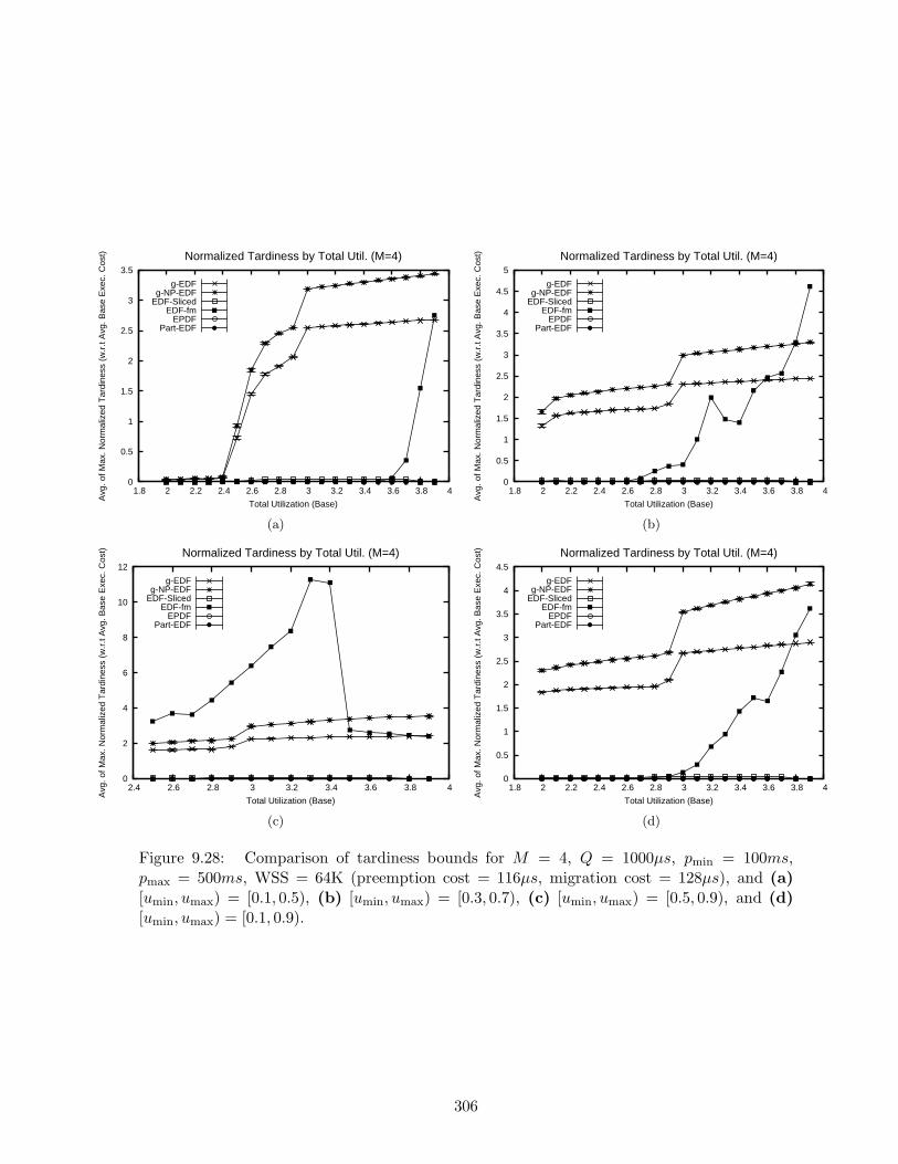
0

0.5

1

1.5

2

2.5

3

3.5

1.8 2 2.2 2.4 2.6 2.8 3 3.2 3.4 3.6 3.8 4

Avg

. of M

ax. N

orm

aliz

ed T

ardi

ness

(w

.r.t

Avg

. Bas

e E

xec.

Cos

t)



g-EDFg-NP-EDF

EDF-SlicedEDF-fm

EPDFPart-EDF

(a)

0

0.5

1

1.5

2

2.5

3

3.5

4

4.5

5

1.8 2 2.2 2.4 2.6 2.8 3 3.2 3.4 3.6 3.8 4

Avg

. of M

ax. N

orm

aliz

ed T

ardi

ness

(w

.r.t

Avg

. Bas

e E

xec.

Cos

t)



g-EDFg-NP-EDF

EDF-SlicedEDF-fm

EPDFPart-EDF

(b)

0

2

4

6

8

10

12

2.4 2.6 2.8 3 3.2 3.4 3.6 3.8 4

Avg

. of M

ax. N

orm

aliz

ed T

ardi

ness

(w

.r.t

Avg

. Bas

e E

xec.

Cos

t)



g-EDFg-NP-EDF

EDF-SlicedEDF-fm

EPDFPart-EDF

(c)

0

0.5

1

1.5

2

2.5

3

3.5

4

4.5

1.8 2 2.2 2.4 2.6 2.8 3 3.2 3.4 3.6 3.8 4

Avg

. of M

ax. N

orm

aliz

ed T

ardi

ness

(w

.r.t

Avg

. Bas

e E

xec.

Cos

t)



g-EDFg-NP-EDF

EDF-SlicedEDF-fm

EPDFPart-EDF

(d)


306

0

2000

4000

6000

8000

10000

1.8 2 2.2 2.4 2.6 2.8 3 3.2 3.4 3.6 3.8 4

Num

ber

of S

ched

ulab

le T

ask

Set

s




g-NP-EDFEDF-Sliced

EDF-fmEPDF

P-EDF

(a)

0

2000

4000

6000

8000

10000

1.8 2 2.2 2.4 2.6 2.8 3 3.2 3.4 3.6 3.8 4

Num

ber

of S

ched

ulab

le T

ask

Set

s




g-NP-EDFEDF-Sliced

EDF-fmEPDF

P-EDF

(b)

0

2000

4000

6000

8000

10000

2.4 2.6 2.8 3 3.2 3.4 3.6 3.8 4

Num

ber

of S

ched

ulab

le T

ask

Set

s




g-NP-EDFEDF-Sliced

EDF-fmEPDF

P-EDF

(c)

0

2000

4000

6000

8000

10000

1.8 2 2.2 2.4 2.6 2.8 3 3.2 3.4 3.6 3.8 4

Num

ber

of S

ched

ulab

le T

ask

Set

s




g-NP-EDFEDF-Sliced

EDF-fmEPDF

P-EDF

(d)


307

0

0.5

1

1.5

2

2.5

3

3.5

1.8 2 2.2 2.4 2.6 2.8 3 3.2 3.4 3.6 3.8 4

Avg

. of M

ax. N

orm

aliz

ed T

ardi

ness

(w

.r.t

Avg

. Bas

e E

xec.

Cos

t)



g-EDFg-NP-EDF

EDF-SlicedEDF-fm

EPDFPart-EDF

(a)

0

0.5

1

1.5

2

2.5

3

3.5

4

4.5

5

1.8 2 2.2 2.4 2.6 2.8 3 3.2 3.4 3.6 3.8 4

Avg

. of M

ax. N

orm

aliz

ed T

ardi

ness

(w

.r.t

Avg

. Bas

e E

xec.

Cos

t)



g-EDFg-NP-EDF

EDF-SlicedEDF-fm

EPDFPart-EDF

(b)

0

2

4

6

8

10

12

2.4 2.6 2.8 3 3.2 3.4 3.6 3.8 4

Avg

. of M

ax. N

orm

aliz

ed T

ardi

ness

(w

.r.t

Avg

. Bas

e E

xec.

Cos

t)



g-EDFg-NP-EDF

EDF-SlicedEDF-fm

EPDFPart-EDF

(c)

0

0.5

1

1.5

2

2.5

3

3.5

4

4.5

1.8 2 2.2 2.4 2.6 2.8 3 3.2 3.4 3.6 3.8 4

Avg

. of M

ax. N

orm

aliz

ed T

ardi

ness

(w

.r.t

Avg

. Bas

e E

xec.

Cos

t)



g-EDFg-NP-EDF

EDF-SlicedEDF-fm

EPDFPart-EDF

(d)


308

0

2000

4000

6000

8000

10000

1.8 2 2.2 2.4 2.6 2.8 3 3.2 3.4 3.6 3.8 4

Num

ber

of S

ched

ulab

le T

ask

Set

s




g-NP-EDFEDF-Sliced

EDF-fmEPDF

P-EDF

(a)

0

2000

4000

6000

8000

10000

1.8 2 2.2 2.4 2.6 2.8 3 3.2 3.4 3.6 3.8 4N

umbe

r of

Sch

edul

able

Tas

k S

ets




g-NP-EDFEDF-Sliced

EDF-fmEPDF

P-EDF

(b)

0

2000

4000

6000

8000

10000

1.8 2 2.2 2.4 2.6 2.8 3 3.2 3.4 3.6 3.8 4

Num

ber

of S

ched

ulab

le T

ask

Set

s




g-NP-EDFEDF-Sliced

EDF-fmEPDF

P-EDF

(c)


309

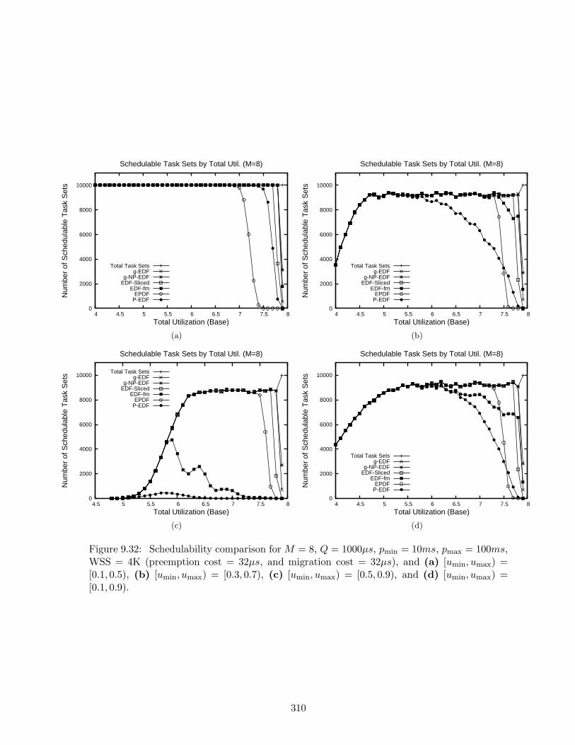
0

2000

4000

6000

8000

10000

4 4.5 5 5.5 6 6.5 7 7.5 8

Num

ber

of S

ched

ulab

le T

ask

Set

s




g-NP-EDFEDF-Sliced

EDF-fmEPDF

P-EDF

(a)

0

2000

4000

6000

8000

10000

4 4.5 5 5.5 6 6.5 7 7.5 8

Num

ber

of S

ched

ulab

le T

ask

Set

s




g-NP-EDFEDF-Sliced

EDF-fmEPDF

P-EDF

(b)

0

2000

4000

6000

8000

10000

4.5 5 5.5 6 6.5 7 7.5 8

Num

ber

of S

ched

ulab

le T

ask

Set

s




g-NP-EDFEDF-Sliced

EDF-fmEPDF

P-EDF

(c)

0

2000

4000

6000

8000

10000

4 4.5 5 5.5 6 6.5 7 7.5 8

Num

ber

of S

ched

ulab

le T

ask

Set

s




g-NP-EDFEDF-Sliced

EDF-fmEPDF

P-EDF

(d)


310

-2

-1

0

1

2

3

4

4 4.5 5 5.5 6 6.5 7 7.5 8

Avg

. of M

ax. N

orm

aliz

ed T

ardi

ness

(w

.r.t

Avg

. Bas

e E

xec.

Cos

t)



g-EDFg-NP-EDF

EDF-SlicedEDF-fm

EPDFPart-EDF

(a)

-2

0

2

4

6

8

10

12

4 4.5 5 5.5 6 6.5 7 7.5 8

Avg

. of M

ax. N

orm

aliz

ed T

ardi

ness

(w

.r.t

Avg

. Bas

e E

xec.

Cos

t)



g-EDFg-NP-EDF

EDF-SlicedEDF-fm

EPDFPart-EDF

(b)

-20

-15

-10

-5

0

5

10

15

20

4.5 5 5.5 6 6.5 7 7.5 8

Avg

. of M

ax. N

orm

aliz

ed T

ardi

ness

(w

.r.t

Avg

. Bas

e E

xec.

Cos

t)



g-EDFg-NP-EDF

EDF-SlicedEDF-fm

EPDFPart-EDF

(c)

-1

0

1

2

3

4

5

6

7

8

9

4 4.5 5 5.5 6 6.5 7 7.5 8

Avg

. of M

ax. N

orm

aliz

ed T

ardi

ness

(w

.r.t

Avg

. Bas

e E

xec.

Cos

t)



g-EDFg-NP-EDF

EDF-SlicedEDF-fm

EPDFPart-EDF

(d)


311

0

2000

4000

6000

8000

10000

4 4.5 5 5.5 6 6.5 7 7.5 8

Num

ber

of S

ched

ulab

le T

ask

Set

s




g-NP-EDFEDF-Sliced

EDF-fmEPDF

P-EDF

(a)

0

2000

4000

6000

8000

10000

4 4.5 5 5.5 6 6.5 7 7.5 8

Num

ber

of S

ched

ulab

le T

ask

Set

s




g-NP-EDFEDF-Sliced

EDF-fmEPDF

P-EDF

(b)

0

2000

4000

6000

8000

10000

4.5 5 5.5 6 6.5 7 7.5 8

Num

ber

of S

ched

ulab

le T

ask

Set

s




g-NP-EDFEDF-Sliced

EDF-fmEPDF

P-EDF

(c)

0

2000

4000

6000

8000

10000

4 4.5 5 5.5 6 6.5 7 7.5 8

Num

ber

of S

ched

ulab

le T

ask

Set

s




g-NP-EDFEDF-Sliced

EDF-fmEPDF

P-EDF

(d)


312

-0.5

0

0.5

1

1.5

2

2.5

3

3.5

4

4.5

4 4.5 5 5.5 6 6.5 7 7.5 8

Avg

. of M

ax. N

orm

aliz

ed T

ardi

ness

(w

.r.t

Avg

. Bas

e E

xec.

Cos

t)



g-EDFg-NP-EDF

EDF-SlicedEDF-fm

EPDFPart-EDF

(a)

-2

0

2

4

6

8

10

12

14

4 4.5 5 5.5 6 6.5 7 7.5 8

Avg

. of M

ax. N

orm

aliz

ed T

ardi

ness

(w

.r.t

Avg

. Bas

e E

xec.

Cos

t)



g-EDFg-NP-EDF

EDF-SlicedEDF-fm

EPDFPart-EDF

(b)

0

2

4

6

8

10

12

14

4.5 5 5.5 6 6.5 7 7.5 8

Avg

. of M

ax. N

orm

aliz

ed T

ardi

ness

(w

.r.t

Avg

. Bas

e E

xec.

Cos

t)



g-EDFg-NP-EDF

EDF-SlicedEDF-fm

EPDFPart-EDF

(c)

-1

0

1

2

3

4

5

6

7

8

9

10

4 4.5 5 5.5 6 6.5 7 7.5 8

Avg

. of M

ax. N

orm

aliz

ed T

ardi

ness

(w

.r.t

Avg

. Bas

e E

xec.

Cos

t)



g-EDFg-NP-EDF

EDF-SlicedEDF-fm

EPDFPart-EDF

(d)


313

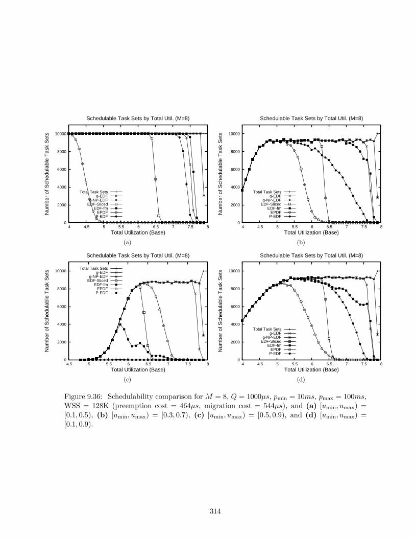
0

2000

4000

6000

8000

10000

4 4.5 5 5.5 6 6.5 7 7.5 8

Num

ber

of S

ched

ulab

le T

ask

Set

s




g-NP-EDFEDF-Sliced

EDF-fmEPDF

P-EDF

(a)

0

2000

4000

6000

8000

10000

4 4.5 5 5.5 6 6.5 7 7.5 8

Num

ber

of S

ched

ulab

le T

ask

Set

s




g-NP-EDFEDF-Sliced

EDF-fmEPDF

P-EDF

(b)

0

2000

4000

6000

8000

10000

4.5 5 5.5 6 6.5 7 7.5 8

Num

ber

of S

ched

ulab

le T

ask

Set

s




g-NP-EDFEDF-Sliced

EDF-fmEPDF

P-EDF

(c)

0

2000

4000

6000

8000

10000

4 4.5 5 5.5 6 6.5 7 7.5 8

Num

ber

of S

ched

ulab

le T

ask

Set

s




g-NP-EDFEDF-Sliced

EDF-fmEPDF

P-EDF

(d)


314

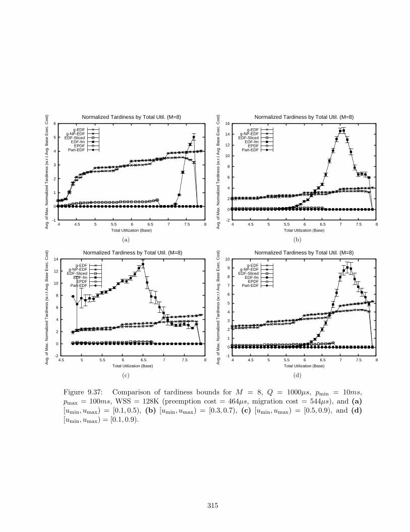
-1

0

1

2

3

4

5

6

4 4.5 5 5.5 6 6.5 7 7.5 8

Avg

. of M

ax. N

orm

aliz

ed T

ardi

ness

(w

.r.t

Avg

. Bas

e E

xec.

Cos

t)



g-EDFg-NP-EDF

EDF-SlicedEDF-fm

EPDFPart-EDF

(a)

-2

0

2

4

6

8

10

12

14

16

4 4.5 5 5.5 6 6.5 7 7.5 8

Avg

. of M

ax. N

orm

aliz

ed T

ardi

ness

(w

.r.t

Avg

. Bas

e E

xec.

Cos

t)



g-EDFg-NP-EDF

EDF-SlicedEDF-fm

EPDFPart-EDF

(b)

-2

0

2

4

6

8

10

12

14

4.5 5 5.5 6 6.5 7 7.5 8

Avg

. of M

ax. N

orm

aliz

ed T

ardi

ness

(w

.r.t

Avg

. Bas

e E

xec.

Cos

t)



g-EDFg-NP-EDF

EDF-SlicedEDF-fm

EPDFPart-EDF

(c)

-1

0

1

2

3

4

5

6

7

8

9

10

4 4.5 5 5.5 6 6.5 7 7.5 8

Avg

. of M

ax. N

orm

aliz

ed T

ardi

ness

(w

.r.t

Avg

. Bas

e E

xec.

Cos

t)



g-EDFg-NP-EDF

EDF-SlicedEDF-fm

EPDFPart-EDF

(d)


315

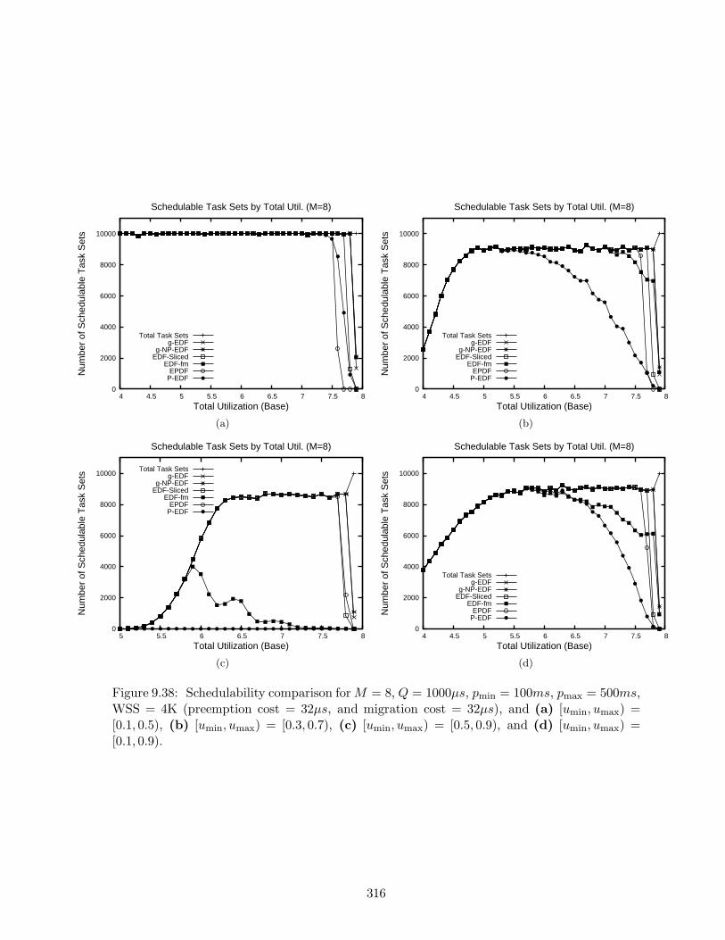
0

2000

4000

6000

8000

10000

4 4.5 5 5.5 6 6.5 7 7.5 8

Num

ber

of S

ched

ulab

le T

ask

Set

s




g-NP-EDFEDF-Sliced

EDF-fmEPDF

P-EDF

(a)

0

2000

4000

6000

8000

10000

4 4.5 5 5.5 6 6.5 7 7.5 8

Num

ber

of S

ched

ulab

le T

ask

Set

s




g-NP-EDFEDF-Sliced

EDF-fmEPDF

P-EDF

(b)

0

2000

4000

6000

8000

10000

5 5.5 6 6.5 7 7.5 8

Num

ber

of S

ched

ulab

le T

ask

Set

s




g-NP-EDFEDF-Sliced

EDF-fmEPDF

P-EDF

(c)

0

2000

4000

6000

8000

10000

4 4.5 5 5.5 6 6.5 7 7.5 8

Num

ber

of S

ched

ulab

le T

ask

Set

s




g-NP-EDFEDF-Sliced

EDF-fmEPDF

P-EDF

(d)


316

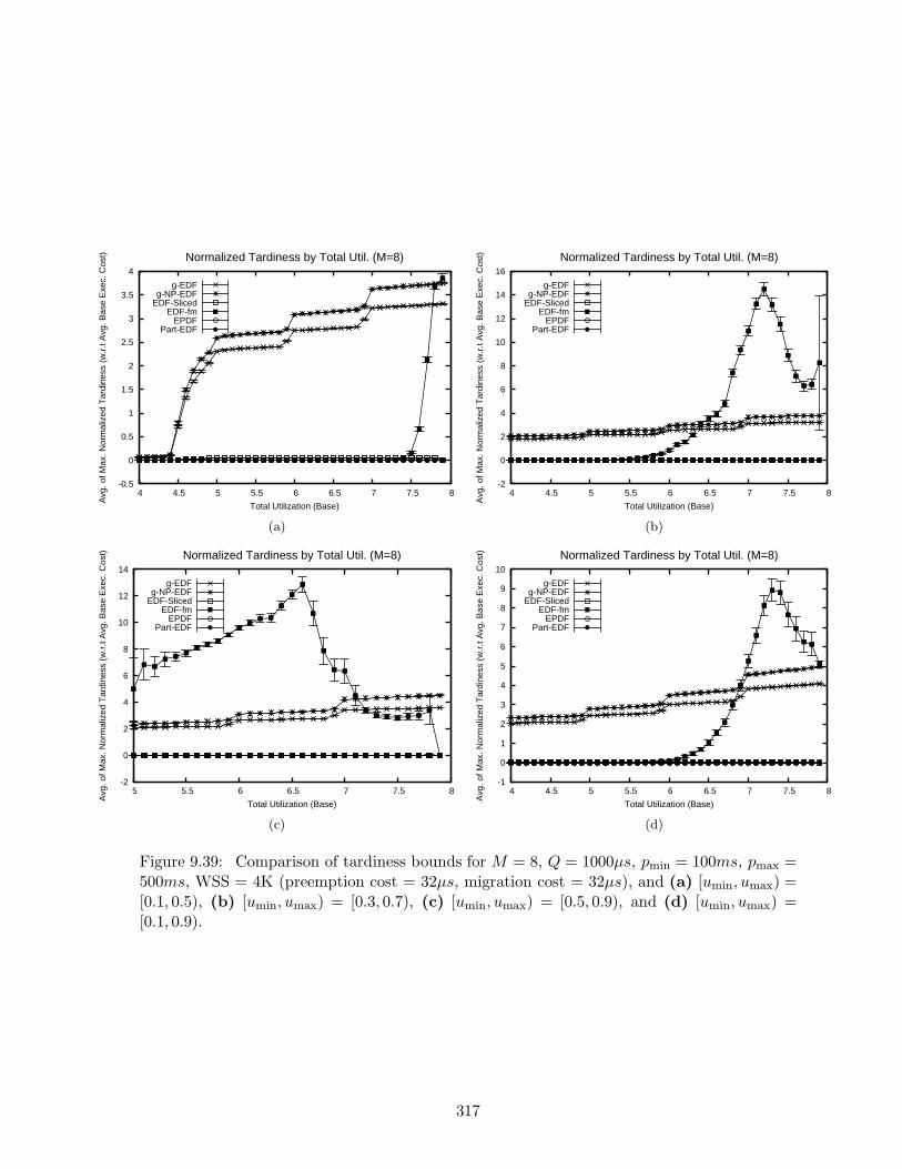
-0.5

0

0.5

1

1.5

2

2.5

3

3.5

4

4 4.5 5 5.5 6 6.5 7 7.5 8

Avg

. of M

ax. N

orm

aliz

ed T

ardi

ness

(w

.r.t

Avg

. Bas

e E

xec.

Cos

t)



g-EDFg-NP-EDF

EDF-SlicedEDF-fm

EPDFPart-EDF

(a)

-2

0

2

4

6

8

10

12

14

16

4 4.5 5 5.5 6 6.5 7 7.5 8

Avg

. of M

ax. N

orm

aliz

ed T

ardi

ness

(w

.r.t

Avg

. Bas

e E

xec.

Cos

t)



g-EDFg-NP-EDF

EDF-SlicedEDF-fm

EPDFPart-EDF

(b)

-2

0

2

4

6

8

10

12

14

5 5.5 6 6.5 7 7.5 8

Avg

. of M

ax. N

orm

aliz

ed T

ardi

ness

(w

.r.t

Avg

. Bas

e E

xec.

Cos

t)



g-EDFg-NP-EDF

EDF-SlicedEDF-fm

EPDFPart-EDF

(c)

-1

0

1

2

3

4

5

6

7

8

9

10

4 4.5 5 5.5 6 6.5 7 7.5 8

Avg

. of M

ax. N

orm

aliz

ed T

ardi

ness

(w

.r.t

Avg

. Bas

e E

xec.

Cos

t)



g-EDFg-NP-EDF

EDF-SlicedEDF-fm

EPDFPart-EDF

(d)


317

0

2000

4000

6000

8000

10000

4 4.5 5 5.5 6 6.5 7 7.5 8

Num

ber

of S

ched

ulab

le T

ask

Set

s




g-NP-EDFEDF-Sliced

EDF-fmEPDF

P-EDF

(a)

0

2000

4000

6000

8000

10000

4 4.5 5 5.5 6 6.5 7 7.5 8

Num

ber

of S

ched

ulab

le T

ask

Set

s




g-NP-EDFEDF-Sliced

EDF-fmEPDF

P-EDF

(b)

0

2000

4000

6000

8000

10000

5 5.5 6 6.5 7 7.5 8

Num

ber

of S

ched

ulab

le T

ask

Set

s




g-NP-EDFEDF-Sliced

EDF-fmEPDF

P-EDF

(c)

0

2000

4000

6000

8000

10000

4 4.5 5 5.5 6 6.5 7 7.5 8

Num

ber

of S

ched

ulab

le T

ask

Set

s




g-NP-EDFEDF-Sliced

EDF-fmEPDF

P-EDF

(d)


318

-0.5

0

0.5

1

1.5

2

2.5

3

3.5

4

4 4.5 5 5.5 6 6.5 7 7.5 8

Avg

. of M

ax. N

orm

aliz

ed T

ardi

ness

(w

.r.t

Avg

. Bas

e E

xec.

Cos

t)



g-EDFg-NP-EDF

EDF-SlicedEDF-fm

EPDFPart-EDF

(a)

-2

0

2

4

6

8

10

12

14

16

4 4.5 5 5.5 6 6.5 7 7.5 8

Avg

. of M

ax. N

orm

aliz

ed T

ardi

ness

(w

.r.t

Avg

. Bas

e E

xec.

Cos

t)



g-EDFg-NP-EDF

EDF-SlicedEDF-fm

EPDFPart-EDF

(b)

0

2

4

6

8

10

12

14

5 5.5 6 6.5 7 7.5 8

Avg

. of M

ax. N

orm

aliz

ed T

ardi

ness

(w

.r.t

Avg

. Bas

e E

xec.

Cos

t)



g-EDFg-NP-EDF

EDF-SlicedEDF-fm

EPDFPart-EDF

(c)

-1

0

1

2

3

4

5

6

7

8

9

10

4 4.5 5 5.5 6 6.5 7 7.5 8

Avg

. of M

ax. N

orm

aliz

ed T

ardi

ness

(w

.r.t

Avg

. Bas

e E

xec.

Cos

t)



g-EDFg-NP-EDF

EDF-SlicedEDF-fm

EPDFPart-EDF

(d)


319

0

2000

4000

6000

8000

10000

4 4.5 5 5.5 6 6.5 7 7.5 8

Num

ber

of S

ched

ulab

le T

ask

Set

s




g-NP-EDFEDF-Sliced

EDF-fmEPDF

P-EDF

(a)

0

2000

4000

6000

8000

10000

4 4.5 5 5.5 6 6.5 7 7.5 8

Num

ber

of S

ched

ulab

le T

ask

Set

s




g-NP-EDFEDF-Sliced

EDF-fmEPDF

P-EDF

(b)

0

2000

4000

6000

8000

10000

5 5.5 6 6.5 7 7.5 8

Num

ber

of S

ched

ulab

le T

ask

Set

s




g-NP-EDFEDF-Sliced

EDF-fmEPDF

P-EDF

(c)

0

2000

4000

6000

8000

10000

4 4.5 5 5.5 6 6.5 7 7.5 8

Num

ber

of S

ched

ulab

le T

ask

Set

s




g-NP-EDFEDF-Sliced

EDF-fmEPDF

P-EDF

(d)


320

-0.5

0

0.5

1

1.5

2

2.5

3

3.5

4

4.5

4 4.5 5 5.5 6 6.5 7 7.5 8

Avg

. of M

ax. N

orm

aliz

ed T

ardi

ness

(w

.r.t

Avg

. Bas

e E

xec.

Cos

t)



g-EDFg-NP-EDF

EDF-SlicedEDF-fm

EPDFPart-EDF

(a)

-2

0

2

4

6

8

10

12

14

16

4 4.5 5 5.5 6 6.5 7 7.5 8

Avg

. of M

ax. N

orm

aliz

ed T

ardi

ness

(w

.r.t

Avg

. Bas

e E

xec.

Cos

t)



g-EDFg-NP-EDF

EDF-SlicedEDF-fm

EPDFPart-EDF

(b)

-10

-5

0

5

10

15

5 5.5 6 6.5 7 7.5 8

Avg

. of M

ax. N

orm

aliz

ed T

ardi

ness

(w

.r.t

Avg

. Bas

e E

xec.

Cos

t)



g-EDFg-NP-EDF

EDF-SlicedEDF-fm

EPDFPart-EDF

(c)

-1

0

1

2

3

4

5

6

7

8

9

10

4 4.5 5 5.5 6 6.5 7 7.5 8

Avg

. of M

ax. N

orm

aliz

ed T

ardi

ness

(w

.r.t

Avg

. Bas

e E

xec.

Cos

t)



g-EDFg-NP-EDF

EDF-SlicedEDF-fm

EPDFPart-EDF

(d)


321

0

2000

4000

6000

8000

10000

4 4.5 5 5.5 6 6.5 7 7.5 8

Num

ber

of S

ched

ulab

le T

ask

Set

s




g-NP-EDFEDF-Sliced

EDF-fmEPDF

P-EDF

(a)

0

2000

4000

6000

8000

10000

4 4.5 5 5.5 6 6.5 7 7.5 8N

umbe

r of

Sch

edul

able

Tas

k S

ets




g-NP-EDFEDF-Sliced

EDF-fmEPDF

P-EDF

(b)

0

2000

4000

6000

8000

10000

4 4.5 5 5.5 6 6.5 7 7.5 8

Num

ber

of S

ched

ulab

le T

ask

Set

s




g-NP-EDFEDF-Sliced

EDF-fmEPDF

P-EDF

(c)


322

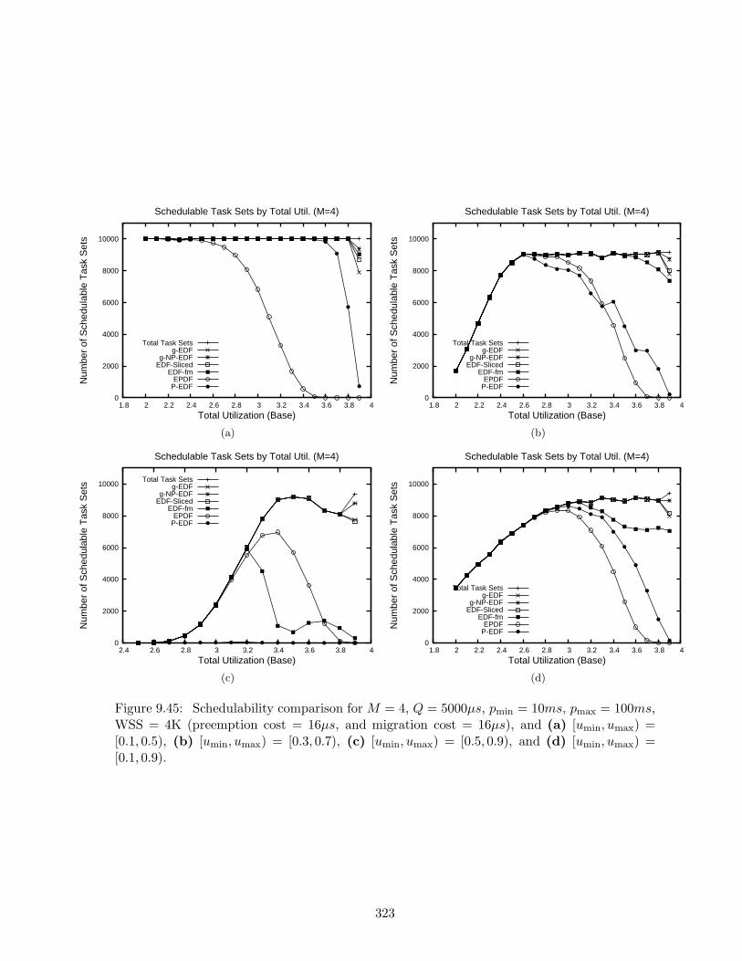
0

2000

4000

6000

8000

10000

1.8 2 2.2 2.4 2.6 2.8 3 3.2 3.4 3.6 3.8 4

Num

ber

of S

ched

ulab

le T

ask

Set

s




g-NP-EDFEDF-Sliced

EDF-fmEPDF

P-EDF

(a)

0

2000

4000

6000

8000

10000

1.8 2 2.2 2.4 2.6 2.8 3 3.2 3.4 3.6 3.8 4

Num

ber

of S

ched

ulab

le T

ask

Set

s




g-NP-EDFEDF-Sliced

EDF-fmEPDF

P-EDF

(b)

0

2000

4000

6000

8000

10000

2.4 2.6 2.8 3 3.2 3.4 3.6 3.8 4

Num

ber

of S

ched

ulab

le T

ask

Set

s




g-NP-EDFEDF-Sliced

EDF-fmEPDF

P-EDF

(c)

0

2000

4000

6000

8000

10000

1.8 2 2.2 2.4 2.6 2.8 3 3.2 3.4 3.6 3.8 4

Num

ber

of S

ched

ulab

le T

ask

Set

s




g-NP-EDFEDF-Sliced

EDF-fmEPDF

P-EDF

(d)


323

0

2000

4000

6000

8000

10000

1.8 2 2.2 2.4 2.6 2.8 3 3.2 3.4 3.6 3.8 4

Num

ber

of S

ched

ulab

le T

ask

Set

s




g-NP-EDFEDF-Sliced

EDF-fmEPDF

P-EDF

(a)

0

2000

4000

6000

8000

10000

1.8 2 2.2 2.4 2.6 2.8 3 3.2 3.4 3.6 3.8 4

Num

ber

of S

ched

ulab

le T

ask

Set

s




g-NP-EDFEDF-Sliced

EDF-fmEPDF

P-EDF

(b)

0

2000

4000

6000

8000

10000

2.4 2.6 2.8 3 3.2 3.4 3.6 3.8 4

Num

ber

of S

ched

ulab

le T

ask

Set

s




g-NP-EDFEDF-Sliced

EDF-fmEPDF

P-EDF

(c)

0

2000

4000

6000

8000

10000

1.8 2 2.2 2.4 2.6 2.8 3 3.2 3.4 3.6 3.8 4

Num

ber

of S

ched

ulab

le T

ask

Set

s




g-NP-EDFEDF-Sliced

EDF-fmEPDF

P-EDF

(d)


324

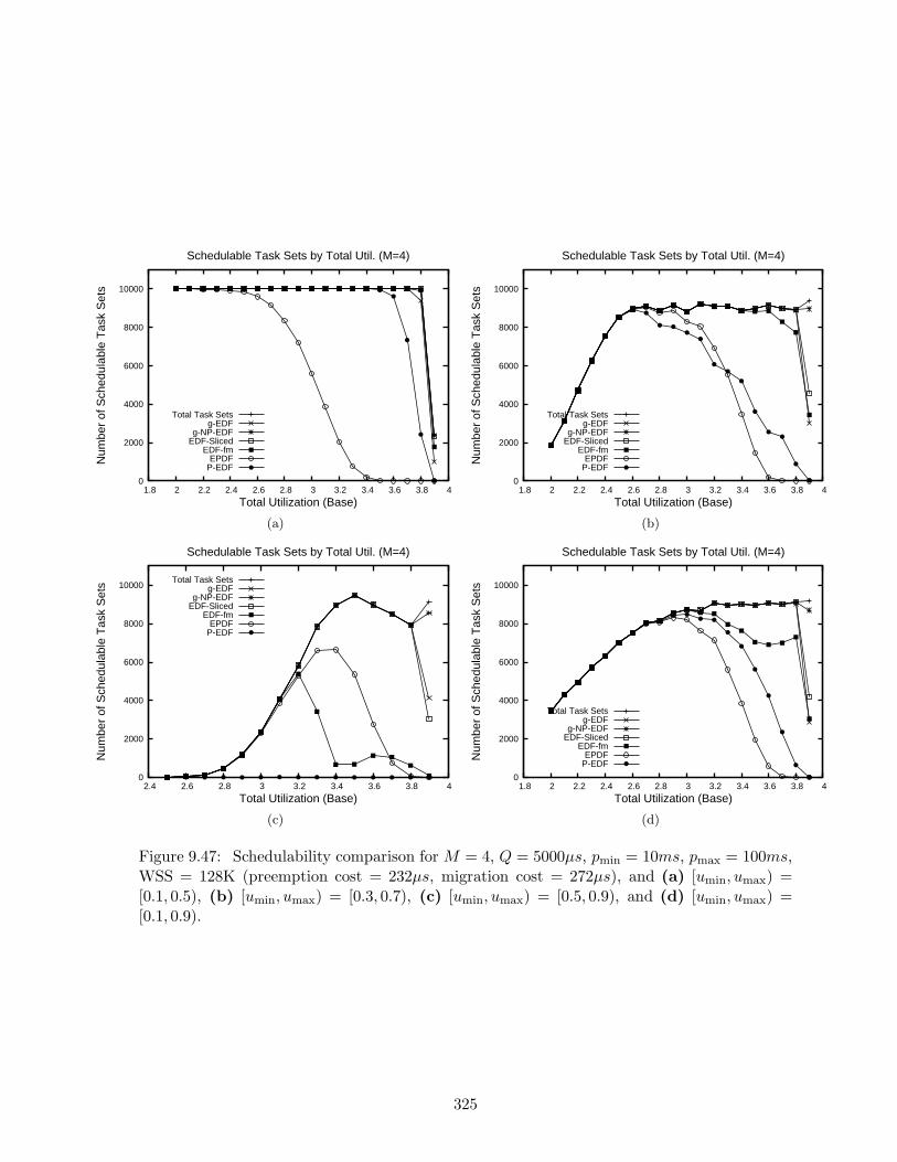
0

2000

4000

6000

8000

10000

1.8 2 2.2 2.4 2.6 2.8 3 3.2 3.4 3.6 3.8 4

Num

ber

of S

ched

ulab

le T

ask

Set

s




g-NP-EDFEDF-Sliced

EDF-fmEPDF

P-EDF

(a)

0

2000

4000

6000

8000

10000

1.8 2 2.2 2.4 2.6 2.8 3 3.2 3.4 3.6 3.8 4

Num

ber

of S

ched

ulab

le T

ask

Set

s




g-NP-EDFEDF-Sliced

EDF-fmEPDF

P-EDF

(b)

0

2000

4000

6000

8000

10000

2.4 2.6 2.8 3 3.2 3.4 3.6 3.8 4

Num

ber

of S

ched

ulab

le T

ask

Set

s




g-NP-EDFEDF-Sliced

EDF-fmEPDF

P-EDF

(c)

0

2000

4000

6000

8000

10000

1.8 2 2.2 2.4 2.6 2.8 3 3.2 3.4 3.6 3.8 4

Num

ber

of S

ched

ulab

le T

ask

Set

s




g-NP-EDFEDF-Sliced

EDF-fmEPDF

P-EDF

(d)


325

0

2000

4000

6000

8000

10000

1.8 2 2.2 2.4 2.6 2.8 3 3.2 3.4 3.6 3.8 4

Num

ber

of S

ched

ulab

le T

ask

Set

s




g-NP-EDFEDF-Sliced

EDF-fmEPDF

P-EDF

(a)

0

2000

4000

6000

8000

10000

1.8 2 2.2 2.4 2.6 2.8 3 3.2 3.4 3.6 3.8 4

Num

ber

of S

ched

ulab

le T

ask

Set

s




g-NP-EDFEDF-Sliced

EDF-fmEPDF

P-EDF

(b)

0

2000

4000

6000

8000

10000

2.4 2.6 2.8 3 3.2 3.4 3.6 3.8 4

Num

ber

of S

ched

ulab

le T

ask

Set

s




g-NP-EDFEDF-Sliced

EDF-fmEPDF

P-EDF

(c)

0

2000

4000

6000

8000

10000

1.8 2 2.2 2.4 2.6 2.8 3 3.2 3.4 3.6 3.8 4

Num

ber

of S

ched

ulab

le T

ask

Set

s




g-NP-EDFEDF-Sliced

EDF-fmEPDF

P-EDF

(d)


326

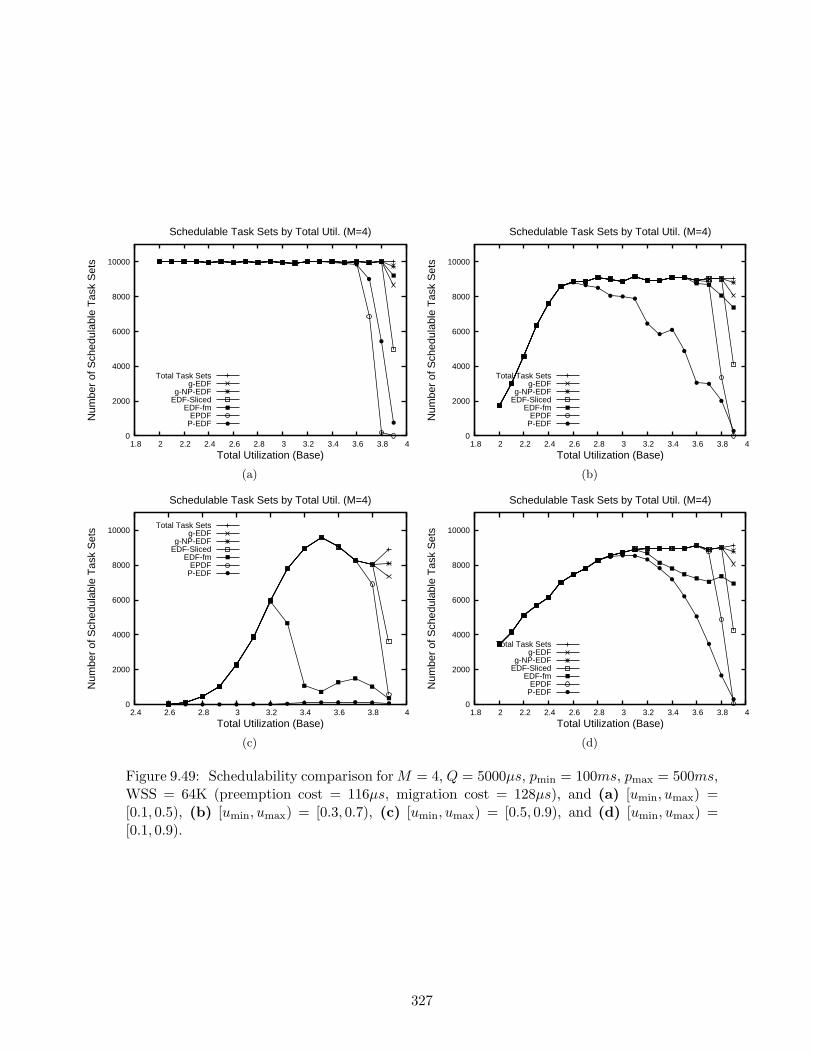
0

2000

4000

6000

8000

10000

1.8 2 2.2 2.4 2.6 2.8 3 3.2 3.4 3.6 3.8 4

Num

ber

of S

ched

ulab

le T

ask

Set

s




g-NP-EDFEDF-Sliced

EDF-fmEPDF

P-EDF

(a)

0

2000

4000

6000

8000

10000

1.8 2 2.2 2.4 2.6 2.8 3 3.2 3.4 3.6 3.8 4

Num

ber

of S

ched

ulab

le T

ask

Set

s




g-NP-EDFEDF-Sliced

EDF-fmEPDF

P-EDF

(b)

0

2000

4000

6000

8000

10000

2.4 2.6 2.8 3 3.2 3.4 3.6 3.8 4

Num

ber

of S

ched

ulab

le T

ask

Set

s




g-NP-EDFEDF-Sliced

EDF-fmEPDF

P-EDF

(c)

0

2000

4000

6000

8000

10000

1.8 2 2.2 2.4 2.6 2.8 3 3.2 3.4 3.6 3.8 4

Num

ber

of S

ched

ulab

le T

ask

Set

s




g-NP-EDFEDF-Sliced

EDF-fmEPDF

P-EDF

(d)


327

0

2000

4000

6000

8000

10000

1.8 2 2.2 2.4 2.6 2.8 3 3.2 3.4 3.6 3.8 4

Num

ber

of S

ched

ulab

le T

ask

Set

s




g-NP-EDFEDF-Sliced

EDF-fmEPDF

P-EDF

(a)

0

2000

4000

6000

8000

10000

1.8 2 2.2 2.4 2.6 2.8 3 3.2 3.4 3.6 3.8 4

Num

ber

of S

ched

ulab

le T

ask

Set

s




g-NP-EDFEDF-Sliced

EDF-fmEPDF

P-EDF

(b)

0

2000

4000

6000

8000

10000

2.4 2.6 2.8 3 3.2 3.4 3.6 3.8 4

Num

ber

of S

ched

ulab

le T

ask

Set

s




g-NP-EDFEDF-Sliced

EDF-fmEPDF

P-EDF

(c)

0

2000

4000

6000

8000

10000

1.8 2 2.2 2.4 2.6 2.8 3 3.2 3.4 3.6 3.8 4

Num

ber

of S

ched

ulab

le T

ask

Set

s




g-NP-EDFEDF-Sliced

EDF-fmEPDF

P-EDF

(d)


328

9.5 Summary

In this chapter, we presented a simulation-based evaluation of p-EDF and the scheduling al-

gorithms considered in this dissertation after accounting for some realistic overheads. Before

presenting our evaluation, we described some significant practical overheads that can delay ap-

plication tasks, showed how to account for those overheads under the different scheduling algo-

rithms, and described the procedure we used to obtain some realistic values for the overheads.

These real overheads were then used to drive an empirical study involving randomly-generated

task sets to determine the percentage of task sets for which each algorithm can guarantee

bounded tardiness and the maximum tardiness bound guaranteed on average. The results of

our studies show that with respect to the task sets generated, the algorithms considered in this

dissertation can guarantee bounded tardiness for a significant percentage of task sets that are

not schedulable in a hard real-time sense. Furthermore, for each algorithm, conditions exist

in which it may be the preferred choice.

329

Chapter 10

Conclusions and Future Work

In real-time systems research, enabling cost-effective implementations of soft real-time appli-

cations on multiprocessors is of growing importance. This is due to both an increase in the

availability of affordable multiprocessor platforms, and the prevalence of applications with

workloads necessitating multiprocessors and for which soft real-time guarantees are sufficient.

One crucial aspect of a cost-effective system design lies in the careful and efficient allocation

of system resources to application tasks — the task of the system scheduler.

However, real-time scheduling theory has not kept pace in providing needed tools and

techniques for multiprocessor-based soft real-time systems. Specifically, known scheduling

algorithms either are theoretically optimal but can incur significant overhead, which can reduce

the amount of useful work accomplished, or are non-optimal and have been analyzed only in the

context of hard real-time systems, and as such, can require that the workload be restricted to

roughly 50% of the available processing capacity. Thus, state-of-the-art scheduling techniques

can be overkill for soft real-time systems, which can tolerate occasional or bounded deadline

misses, and hence, allow for a trade-off between timeliness and improved resource utilization.

In this dissertation, we attempted to bridge this gap by analyzing some known algorithms

in the context of guaranteeing bounded tardiness, designing a new algorithm specifically for

soft real-time systems and analyzing it, and analyzing some relaxed variants of optimal Pfair

algorithms. In this chapter, we conclude by summarizing the results presented in earlier

chapters, and by enumerating and discussing some challenges that remain to be addressed.

10.1 Summary of Results

The thesis that this dissertation strived to support is that processor utilization can be im-

proved on multiprocessors while providing non-trivial soft real-time guarantees for different

recurrent soft real-time applications, whose preemption and migration overheads can span dif-

ferent ranges and whose tolerances to tardiness are different, by designing new algorithms,

simplifying optimal algorithms, and developing new validation tests. In this section, we discuss

results presented in support of this thesis.

In Chapter 4, we provided counterexamples that showed that improved resource utilization

is not be possible for recurrent real-time task systems under partitioning algorithms or full-

migration, static-priority algorithms even if bounded tardiness can be tolerated. Hence, in

establishing our thesis, we focused on algorithms that use dynamic priorities (either restricted

or unrestricted) and that allow some degree of migration. (Static-priority algorithms were not

considered in general because as discussed in Section 1.4.2.2, within a migration class, such

algorithms are strictly less powerful than and incur almost equal overhead as dynamic-priority

algorithms.)

Analysis of preemptive and non-preemptive global EDF (g-EDF and g-NP-EDF). The

elimination of partitioned and static-priority algorithms leaves the well-known EDF algorithm

as an obvious first choice for consideration in soft real-time systems. Unlike optimal Pfair

algorithms, EDF is a restricted dynamic-priority algorithm and incurs significantly less over-

head. However, EDF suffers from the drawback that its schedulable utilization bound is low on

multiprocessors. Specifically, on M processors, the worst-case schedulable utilization bound of

g-EDF cannot exceed (M +1)/2 and the corresponding value is still lower for g-NP-EDF. Thus,

g-EDF and g-NP-EDF offered significant scope in improving processor utilization for soft real-

time systems if bounded tardiness that is reasonable can be guaranteed under them. Motivated

by this prospect, in Chapter 4, we considered determining the extent to which deadlines can

be missed by otherwise feasible task systems under g-EDF and g-NP-EDF. We showed that on

M processors, g-EDF and g-NP-EDF can guarantee tardiness bounds of∑Λ

i=1 εi−emin

M−∑Λ−1

i=1 µi

+ ek and∑Λ+1

i=1 εi−emin

M−∑Λ

i=1 µi+ ek, respectively, for each task Tk of every task system τ with Usum ≤ M . (εi,

µi, and Λ are defined in Section 4.2.) Though we do not believe the above bounds to be tight

in general, as a special case, we derived a tardiness bound of (emax + ek)/2 for two-processor

systems under g-EDF, and provided a counterexample to show that this result is close to being

331

tight. Further, as discussed in Chapter 4, the bounds are reasonable unless task utilizations

and the number of processors are both high. Specifically, if task utilizations are at most 0.75

or the number of processors is at most eight, then the tardiness bounds guaranteed can be

expected to be within tolerable limits. We expect most practical systems to adhere to these

limits, and hence, the bounds derived should suffice for practical purposes.

Design and analysis of EDF-fm. Though migration and other overheads are lower under

EDF than under optimal Pfair algorithms, migrations are still unrestricted. (Note that though

g-NP-EDF eliminates job migrations by eliminating job preemptions, task migrations are still

unrestricted.) This may be unappealing to some systems, especially to those with high inter-

and intra-job migration costs and that cannot be partitioned. To address this issue, in Chap-

ter 5, we proposed an algorithm called EDF-fm, which is based upon EDF, and treads a middle

path, by restricting, but not eliminating, task migrations, and determined a tardiness bound

that can be guaranteed under it. Specifically, under EDF-fm, the ability to migrate is required

for at most M − 1 tasks, and it is sufficient that every such task migrate between two pro-

cessors and at job boundaries only. EDF-fm, like global EDF, can ensure bounded tardiness

to a sporadic task system as long as the available processing capacity is not exceeded, but

unlike global EDF, in general, only if the maximum task utilization, umax, is capped at 0.5. As

umax increases, the ability of EDF-fm to guarantee bounded tardiness decreases. However, in

our simulation studies, we found that on eight processors, EDF-fm could guarantee bounded

tardiness to approximately 60% of the generated task sets even when umax = 1.0.

Apart from deriving a tardiness bound that can be computed in O(N) time but is somewhat

pessimistic, we also derived a pair of iterative formulas for computing near-exact bounds, but

which may require exponential time. In order to lower the tardiness observed in practice,

we proposed several heuristics for assigning to processors those tasks that do not migrate

under EDF-fm, and through extensive simulations, evaluated the efficacy of these heuristics in

lowering the tardiness bound that can be guaranteed. Finally, we presented a simulation-based

evaluation of the accuracy of both the tardiness bounds derived under the heuristic identified

to be the best.

Analysis of relaxed Pfair algorithms. Though g-EDF and g-NP-EDF can guarantee

bounded tardiness to every feasible task system, their tardiness bounds may be beyond the

tolerance limits of some systems. For such systems, algorithms based on Pfair scheduling

332

may be better. Hence, in an attempt to enhance the applicability of Pfair scheduling for soft

real-time systems, we considered relaxing some of its limiting restrictions.

First, we considered the earliest-pseudo-deadline-first (EPDF) Pfair scheduling algorithm,

which avoids the use of tie-breaking rules, and hence, is more efficient than and preferable to

optimal Pfair algorithms. EPDF is especially preferable in dynamic task systems with frequent

changes in task composition or in systems implemented on less-powerful hardware platforms.

However, EPDF is not optimal and deadlines can be missed under it if the number of processors

exceeds two.

Before considering EPDF in the context of soft real-time systems, in Chapter 6, we deter-

mined a sufficient restriction on total system utilization for ensuring that no deadline will be

missed under EPDF. Specifically, we showed that on M processors, EPDF can correctly sched-

ule every task system τ with total utilization at most min(M, λM(λ(1+Wmax)−Wmax)+1+Wmax

λ2(1+Wmax)),

where Wmax = umax(τ) and λ = max(2,⌈

1Wmax

⌉

). Apart from extending the applicability of

EPDF for hard real-time systems, this result should also help in identifying the conditions for

which the soft real-time scheduling results of EPDF are applicable.

In Chapter 7, we presented some soft real-time results for EPDF. We first showed that the

prevailing conjecture that EPDF can guarantee a tardiness bound of one quantum to every

feasible task system is false. Next, improving upon Srinivasan and Anderson’s result that

EPDF can guarantee a tardiness bound of q quanta, where q ≥ 1, to every feasible task system

with Wmax ≤ qq+1 , we showed that a significantly more liberal restriction of Wmax ≤ q+2

q+3 is

sufficient for ensuring the same tardiness bound. Finally, we showed that if Wmax exceeds q+2q+3 ,

then on M processors, a restriction of min(M, ((q+1)Wmax+(q+2))M+((2q+1)Wmax+1)2(q+1)Wmax+2 ) on the total

system utilization of a task system is sufficient to ensure that tardiness for that task system

under EPDF is at most q.

In Chapter 8, we considered relaxing a restriction of Pfair algorithms that periods and

execution costs be specified as integers. We showed that if periods are non-integral, then under

any Pfair algorithm, tardiness is worsened by at most two quanta. For handling non-integer

execution costs, we proposed a simple algorithm called EDF-sliced, under which, each job

(except perhaps the final sub-job) of a task is divided into equal-size sub-jobs that are scheduled

using an NP-EDF scheduling policy. Since NP-EDF does not require integral execution costs,

loss due to rounding is eliminated; tardiness is lowered due to slicing albeit at the expense of

incurring some migration overhead. Hence, for this algorithm, sub-job sizes provide a trade-off

between loss due to migrations and tardiness.

333

Performance evaluation. Finally, in Chapter 9, we presented a simulation-based evalua-

tion of p-EDF and the scheduling algorithms considered in this dissertation after accounting

for some realistic overheads. Before presenting our evaluation, we described some significant

practical overheads that can delay application tasks, showed how to account for those over-

heads under the different scheduling algorithms, and described the procedure we used to obtain

some realistic measurements for the overheads. These real overheads were then used to drive

an empirical study involving randomly-generated task sets to determine the percentage of

task sets for which each algorithm can guarantee bounded tardiness and the tardiness bound

guaranteed on average. The results of our studies showed that with respect to the task sets

generated, bounded tardiness is guaranteed by the algorithms considered in this dissertation

for a significant percentage of task sets that are not schedulable in a hard real-time sense.

Furthermore, for each algorithm, conditions exist in which it may be the preferred choice.

10.2 Other Related Work

In this section, we briefly discuss some work by us related to the topic of this dissertation that

is presented elsewhere but is not included here.

Guaranteeing flexible tardiness bounds. One limitation of the tardiness bounds derived

in this dissertation for the various algorithms is that they are applicable to every task in the

task system under consideration. In other words, any task can incur maximum tardiness. This

may not be acceptable to applications that consist of hard and soft real-time tasks or those

that consist of soft tasks with different tardiness tolerances. In [52], we considered the issue

of supporting task systems with some tasks whose tolerances to tardiness are lower than that

guaranteed under g-EDF. As a solution, we proposed a new scheduling policy, called EDF-hl,

that is a variant of g-EDF, and show that under EDF-hl, any tardiness, including zero tardiness,

can be ensured for a limited number of privileged tasks, and that bounded tardiness can be

guaranteed to the remaining tasks if their utilizations are restricted. EDF-hl reduces to EDF

in the absence of privileged tasks.

Desynchronized Pfair scheduling. In [50], we considered relaxing a restriction of Pfair

scheduling that requires quanta to be synchronized on processors and tasks to be allocated

processor time in units of fixed-sized quanta. We showed that if this requirement, which may

lead to wasted processor time, is relaxed, then under an otherwise optimal Pfair scheduling

334

algorithm, deadlines are missed by at most one quantum only, which is sufficient to provide soft

real-time guarantees. This result can be shown to extend to most prior work on Pfair schedul-

ing: In general, tardiness bounds guaranteed by non-optimal Pfair algorithms are worsened by

at most one quantum only.

Real-Time scheduling on multicore platforms. In [11], we considered the architectural

implications of multicore platforms for scheduling real-time tasks. Multicore architectures

differ from conventional SMP architectures in that multiple processing units, referred to as

processor cores, are housed in a single die. Most multicore designs additionally differ in the

use of shared caches, which can be either on- or off-chip, for the various cores. While a

shared cache has the potential to alleviate migration costs considerably, care must be taken to

ensure that contention from tasks co-scheduled on the various cores does not lead to degraded

performance. In prior work [57], Fedorova et al. observed that contention for shared caches

can be a significant performance bottleneck in multicore systems and proposed a scheduling

algorithm for improving throughput while executing non-real-time applications.

In [11], we considered the issue raised by Fedorova et al. in the context of scheduling

real-time tasks. We proposed a hierarchical approach based on PD2 for scheduling real-time

tasks such that tasks that generate significant memory-to-L2 traffic are discouraged from being

co-scheduled.

10.3 Future Work

We now discuss some of the challenges that remain in the area of multiprocessor-based soft

real-time scheduling.

Tightening the tardiness bounds. Though this dissertation closes the problem of deter-

mining whether global EDF can guarantee bounded tardiness, the question remains as to how

tight the bounds are. As mentioned earlier, our bounds can be high when the average task

utilization is also high, say, above 0.8. While systems with such high-utilization tasks may

be quite rare in practice, the problem of tightening the bounds is, nevertheless, theoretically

important.

Support for other task models. This dissertation has determined some soft real-time

guarantees that can be provided on multiprocessors when the workload is specified for the

335

worst case, does not exceed the available processing capacity, and every job needs to execute

in its entirety. Relaxing these assumptions is an obvious next step in the progression of the

theory of soft real-time scheduling on multiprocessors. As discussed in Chapter 2, considerable

progress has been made in this direction on uniprocessors. Intelligently skipping entire jobs

as in the skippable task model and the (m,k)-firm model, or parts of them, as in the impre-

cise task model, can help in alleviating both long-term and transient short-term overloads for

systems for which worst-case workload specifications are not pessimistic, i.e., when the actual

workload does not deviate significantly from what is specified. On the other hand, for appli-

cations whose workloads can vary widely over time, such as video-conferencing or animation

games, reserving resources based on worst-case specifications can be extremely wasteful. For

such applications, modeling task parameters using probabilistic distributions, and providing

probabilistic guarantees may be better suited. Investigating the efficacy of alternative task

models in the context of multiprocessors remains an open area of research.

Scheduling aperiodic tasks. In Chapter 2, we mentioned that one common approach for

scheduling one-shot, aperiodic tasks that do not conform to any recurrent task model is by

using server tasks. We also mentioned that, in general, a server task is either a periodic

or a sporadic task and is assigned parameters based on the workload needs of the aperiodic

tasks that it serves. However, assigning appropriate parameters for the server tasks is not

simple (due to the variable nature of the aperiodic tasks), and on multiprocessors, is subject

to additional complications than on uniprocessors [110].

While an ability to schedule aperiodic tasks independently in a stand-alone manner appears

to be an attractive alternative, it is fraught with difficulties in ensuring that timing constraints

will be met. This is because, for long-lived systems, offline analysis is simply infeasible due to

the number of tasks, and online validation is not straightforward. Recently, Abdelzaher et al.

considered scheduling aperiodic tasks in a stand-alone manner and developed utilization-based

validation tests that can be applied at run-time for aperiodic tasks both on uniprocessors and

multiprocessors [4, 3]. For this purpose, they defined a notion called synthetic utilization for

aperiodic task sets that is based on the execution requirement and the relative deadline of each

aperiodic task that has arrived, but not completed execution. They showed that, on unipro-

cessors, maintaining synthetic utilization below 1

1+√

12

(58.6%) is sufficient to ensure that no

deadlines will be missed under the deadline-monotonic scheduling policy. On multiprocessors,

they were able to establish a similar bound only for liquid tasks, that is, tasks whose execution

336

requirements are infinitesimal in comparison to their relative deadlines.

On multiprocessors, one alternative to the approach of Abdelzaher et al. is to consider

modeling aperiodic tasks using the extended sporadic task model proposed in Chapter 4, and

use g-EDF as the scheduler. Intuition suggests that if bounded tardiness is tolerable, then the

synthetic utilization can be up to 100% even for non-liquid tasks. It would be interesting to

explore this idea further and evaluate it empirically.

Improving overhead accounting. In Chapter 9, we provided formulas for determining in-

flated WCETs of tasks that are sufficient to account for overheads incurred in practice. While

the overhead costs that we determined are safe, it is unclear whether they are tight. Specif-

ically, our assumption that under global algorithms, a preemption leads to a migration can

be pessimistic. For example, if the number of tasks is small, say M + 1, it appears highly

unlikely that each job preempts some job or each preemption leads to a migration. Further-

more, when jobs miss deadlines, there may be very few preemptions. Since migration costs

are the most significant source of overhead, a better bound on the number of migrations has a

high potential of lowering the amount of inflation needed and improving resource utilization.

However, translating observations or intuitions into general results can be extremely difficult.

To determine whether research in this direction is warranted, it may be helpful to determine,

through simulations, the actual number of preemptions and migrations in schedules generated

for random task sets.

Real-time operating systems. While most of the scheduling algorithms considered in this

dissertation have been implemented in LITMUSRT, currently support is provided only for

scheduling independent, periodic tasks that are static. Adding support for sporadic tasks, and

developing and implementing predictable and efficient techniques for supporting mutual exclu-

sion and precedence constraints, and evaluating the different algorithms for sporadic, dynamic,

and non-independent systems remain to be addressed. Furthermore, our evaluation was for

small- to medium-sized conventional SMPs, and further work is needed for larger platforms,

and other architectures, most notably, multicore platforms, as well. Finally, LITMUSRT cur-

rently uses tick scheduling for non-Pfair algorithms also. For such algorithms, it would be

interesting to explore the viability of tickless implementations, wherein scheduling is entirely

event driven.

337

Hierarchical scheduling for emerging architectures. Though existing multicore chips

have only a modest number of cores, chips with 32 or more cores are expected within a

decade [100]. As the number of cores increases, the complexity of cache configurations also

increases as it may not be feasible for all cores to share a common cache at the lowest level.

Hierarchical organizations, in which subsets of cores share common caches at the lowest level,

with aggregation at higher levels is among the envisioned designs. In such designs, it may

be preferable to limit task migrations to cores sharing lower level caches, and hence, hybrid

scheduling algorithms, with elements of global and partitioned algorithms, may be needed. For

instance, tasks can be partitioned among subsets of processor cores, and a global scheduling

algorithm can be used for each subset. Note that, since the utilization of each task is at most

one, the worst-case loss due to partitioning decreases as processor subset sizes increase. For

example, if P denotes the number of subsets, n the number of cores per subset, and umax the

maximum utilization of any task, then a lower bound on the total utilization of a task set that

cannot be partitioned is given by P ·n−(P−1)·umax.1 (Under traditional partitioning, P = M

and n = 1.) That is, the loss due to partitioning is at most (P − 1) · umax. When n = 4, the

percentage loss due to partitioning is at most (P −1) ·umax/4P , and when umax is slightly over

1/2, this loss reduces to (P −1)/8P , which is 12.5%. In contrast, the corresponding loss under

traditional partitioning could be as high as 50%. Hence, if as expected, the cost of migrating

among processors of the same subset is negligible, hybrid algorithms seem quite attractive.

Further, it may even be possible to improve utilization by using techniques similar to those

used in the design of EDF-fm. In any case, clearly, more research is needed on scheduling

techniques for emerging architectures.

1It may be possible to determine a better bound than that provided here.

338

Appendix A

Remaining Proofs from Chapter 4

In this appendix, we provide the proofs omitted in Chapter 4 and discuss what eliminating

the assumption in (4.1) entails.

A.1 Proof of Lemma 4.4

We first prove Lemma 4.4. (Lemma 4.4 is necessary to establish the bound as given in (4.43) for

g-EDF. Otherwise, only a looser bound of∑Λ

i=1 εi−emin

M−∑Λ

i=1 µi

+ ek can be established. The difference

is in the second term of the denominator. Also, without Lemma 4.4, the bound derived for

two processors would not be close to being tight.)

We begin by extending the notion of “displacements” developed in the context of Pfair

scheduling and subtasks [105] to EDF and jobs.

Displacements. In proving Lemma 4.4, we consider removing one or more jobs from τ .

Note that the resulting task system (composed of the remaining jobs) is still a valid concrete

instantiation of τN . (We can simply assume either that jobs that are of the same task as any

removed job and are released after that job are appropriately renumbered or that the actual

execution costs of removed jobs are reduced to zero.) However, such job removals can cause one

or more of the remaining jobs or job fragments to shift earlier in S. A job fragment is defined

with respect to a schedule, and is a portion of a job, which could potentially be a complete

job, that executes continuously without preemption in some schedule under consideration. As

described below, such shifts due to job removals can be reduced to a set of zero or more disjoint

displacement chains comprised of job fragments of equal lengths. (If a job removal does not

result in any change in the schedule for the remaining jobs, then the number of displacement

chains is zero.) Each displacement chain ∆i is denoted (∆i,1,∆i,2, . . . ,∆i,ni) and is a sequence

of ni equal-length and disjoint displacements. L denotes the length of every job fragment in ev-

ery displacement. Each displacement ∆i,j is a 4-tuple denoted 〈J (i,j), ti,j, J(i,j+1), ti,j+1〉, with

the meaning that job fragment J (i,j+1) scheduled at ti,j+1 displaces fragment J (i,j) scheduled

339

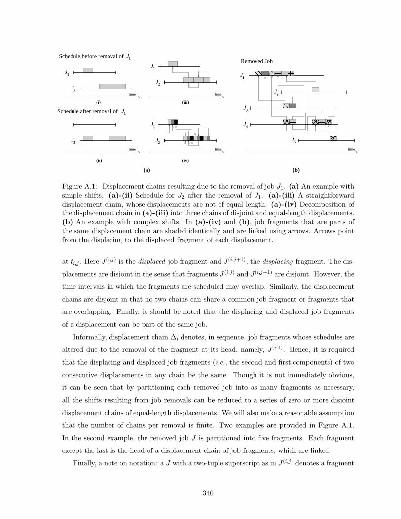
J1

J1

J2

J2

J1

J1

J2

J1

J2

J2

J4

J3

J1

J5

Ú ÚÛ Û Ü ÜÝ Ý

Þ ÞÞ Þß ßß ß

à àà àá áá á

â ââ ââ âã ãã ã ä ää äå åå å æ ææ ææ æç çç ç è èè èé éé é

ê êê êë ëë ë

ì ìí í

î îï ïtime

time time

time

(a) (b)

(i)

(ii) (iv)

(iii)

Schedule before removal of

Schedule after removal of

Removed Job

time

Figure A.1: Displacement chains resulting due to the removal of job J1. (a) An example withsimple shifts. (a)-(ii) Schedule for J2 after the removal of J1. (a)-(iii) A straightforwarddisplacement chain, whose displacements are not of equal length. (a)-(iv) Decomposition ofthe displacement chain in (a)-(iii) into three chains of disjoint and equal-length displacements.(b) An example with complex shifts. In (a)-(iv) and (b), job fragments that are parts ofthe same displacement chain are shaded identically and are linked using arrows. Arrows pointfrom the displacing to the displaced fragment of each displacement.

at ti,j. Here J (i,j) is the displaced job fragment and J (i,j+1), the displacing fragment. The dis-

placements are disjoint in the sense that fragments J (i,j) and J (i,j+1) are disjoint. However, the

time intervals in which the fragments are scheduled may overlap. Similarly, the displacement

chains are disjoint in that no two chains can share a common job fragment or fragments that

are overlapping. Finally, it should be noted that the displacing and displaced job fragments

of a displacement can be part of the same job.

Informally, displacement chain ∆i denotes, in sequence, job fragments whose schedules are

altered due to the removal of the fragment at its head, namely, J (i,1). Hence, it is required

that the displacing and displaced job fragments (i.e., the second and first components) of two

consecutive displacements in any chain be the same. Though it is not immediately obvious,

it can be seen that by partitioning each removed job into as many fragments as necessary,

all the shifts resulting from job removals can be reduced to a series of zero or more disjoint

displacement chains of equal-length displacements. We will also make a reasonable assumption

that the number of chains per removal is finite. Two examples are provided in Figure A.1.

In the second example, the removed job J is partitioned into five fragments. Each fragment

except the last is the head of a displacement chain of job fragments, which are linked.

Finally, a note on notation: a J with a two-tuple superscript as in J (i,j) denotes a fragment

340

of an arbitrary job, and not a fragment of job J .

A few auxiliary lemmas are needed in establishing Lemma 4.4, but first we state the

following simple claim. The claim follows because if jobs all fully preemptable, then jobs in Ψ

are not impacted by those in Ψ. Hence, a non-empty Ψ would contradict the assumption in

(P2).

Claim A.1 If bmax = 0 then Ψ = ∅.

In the lemmas that follow, bmax = 0 holds. Hence, EDF-P-NP reduces to g-EDF. To simplify

description, in the proofs, we will assume that the scheduler is g-EDF.

The lemma below concerns displacements and is quite intuitive. It follows from the work-

conserving nature of g-EDF and our assumption that deadline ties are resolved consistently.

Lemma A.1 If bmax = 0, then for every job removed from τ , the resulting sequence of shifts in

S can be reduced to a set of zero or more displacement chains such that for each displacement

∆i,j in each chain ∆i, ti,j+1 > ti,j, i.e., every displacement is to the left.

We need one more lemma before proving Lemma 4.4.

Lemma A.2 Let [t, t′), where t < t′ ≤ td, be a non-blocking, non-busy interval across which

LAG for Ψ is continually increasing. If bmax = 0, then there exists at least one job J such that

J ’s deadline is at or after t′ and J completes executing at or before t.

Proof: Contrary to the statement of the lemma, assume that there does not exist a job J as

defined. First, we establish a part of the lemma in the following claim.

Claim A.2 There exists at least one job J with deadline at or after t′ that com-

pletes executing before t′.

Proof: Suppose J does not exist. Let t denote the latest of time t and the latest

deadline of any job that completes executing before t′. By our assumption that

a job like J does not exist, t < t′ holds. Because [t, t′) is a non-blocking, non-

busy interval, there does not exist any instant in [t, t′) at which a ready job from

Ψ is waiting. Furthermore, because J does not exist, and by our choice of t′,

there is no instant in [t, t′) at which there is an active job in Ψ that completed

earlier, and hence, is not executing. Thus, there does not exist any instant in

[t, t′) where a task with an active or a pending job in Ψ is not executing. Hence,

341

the total allocation at any instant u in the interval [t, t′) to jobs in Ψ in S is

|{τi|τi,j is in Ψ and is active or pending at u}|, which, by (4.17) and (4.15), is at

least that those jobs receive in PSτ . Therefore, by (4.19), LAG of Ψ at t′ cannot

exceed that at t. This contradicts the fact that LAG for Ψ is continually increasing

in [t, t′). �

Note that J , as specified in the above claim, is not τ`,j. Otherwise, since J completes executing

before its deadline, its tardiness is zero which contradicts (P1). Next, we show that, J com-

pletes executing at or before t. Assume to the contrary, and consider a concrete instantiation

τ ′ of τN obtained by lowering the actual execution time of J such that J does not have to

execute after t. Let S ′ be a schedule for τ ′ such that all ties among jobs are resolved the same

way as in S. Then in S ′, every job in τ ′ except J is scheduled exactly in the same intervals

as in S. This is because no job of Ψ is ready but waiting at any instant in [t, t′) in S, and

hence, the fact that another processor becomes available in [t, t′) due to J not executing in

that interval would not cause additional jobs from Ψ to execute in [t, t′). Since bmax = 0, by

Claim A.1, Ψ = ∅. Hence, no change to the schedule for jobs in Ψ due to the displacement of

jobs in Ψ is possible. Thus, the completion time of every job in Ψ except J will be the same

in both S and S ′. This contradicts (P3), since as explained above, J is not τ`,j. �

We are finally ready to prove Lemma 4.4.

Lemma 4.4 Let [t, t′), where t < t′ ≤ td, be a non-blocking, non-busy interval across which

LAG for Ψ is continually increasing. If bmax = 0, then there exists at least one job J and some

time t such that d(J) ≥ t′, t ≤ t < t′, and J executes continuously in [t, t′).

Proof: By Lemma A.2, there exists a job J ′ such that d(J ′) ≥ t′ and J ′ completes executing

by t. Because J ′ completes executing before its deadline, J ′ is not τ`,j. Otherwise, (P1) is

contradicted. Our proof is by contradiction. Hence, assume (A) below holds.

(A) J as described in the statement of the lemma does not exist.

We show that if (A) holds, then (P2) does not hold, and thereby derive a contradiction.

Consider a concrete instantiation τ ′ of τN obtained from τ by removing J ′. (As explained

above, J ′ is not τ`,j.) Let S ′ be a g-EDF schedule for τ ′ such that ties among jobs are resolved

identically in S and S ′. To show that (P2) is contradicted, we show that if (A) holds, then the

removal of J ′ does not result in any job fragment scheduled after t′ in S (either partially or

342

fully, i.e., the fragment could have commenced execution before t′) to shift left to before t′ in

S ′. This would imply that no job fragments executing after t′, and in particular those of τ`,j,

shift earlier, and hence all jobs scheduled after t′ have the same tardiness in both S and S ′.

Let the removal of J ′ result in a sequence of left shifts for the remaining jobs and let

these shifts be reduced to a set of equal-length, disjoint displacement chains. Our objective

is to show that if some job fragment executing after t′ gets displaced to the left, then (A) is

contradicted. Hence, assume that some job fragment scheduled after t′ undergoes a left shift.

Because there is at least one displacement, the number of displacement chains is at least one,

and by Lemma A.1, we have the following.

(D1) For every displacement ∆i,j in every chain ∆i, ti,j+1 > ti,j.

Also, the fragment at the head of each displacement chain is that of job J ′, whose deadline is

at or after t′. Therefore, by (D1), g-EDF prioritizes J ′ over the job of a fragment later in the

chain. Hence, we have the following.

(D2) The deadline of the job of every fragment involved in every displacement is

at least t′.

Let ∆i,k = 〈J (i,k), ti,k, J(i,k+1), ti,k+1〉 be a displacement such that ti,k+1 + L ≥ t′, where L

is the length of every fragment in the displacement chains under consideration, and ti,k < t′. In

other words, the displacement shifts the job fragment J (i,k+1) either partially or fully to the left

of t′. (By (D1), ti,k < ti,k+1 holds.) If ti,k+1 < t′, then because ti,k+1 +L ≥ t′, J (i,k+1) executes

in S continuously in [ti,k+1, t′), contradicting (A). On the other hand, if ti,k+1 ≥ t′, then we

argue as follows. Because J (i,k+1) is not executing before t′ in S (implied by ti,k+1 ≥ t′),

the non-blocking, non-busy nature of [t, t′) and the fact that J (i,k+1) is executing before t in

S ′ (implied by the displacement ∆i,k and ti,k < t′) imply that J (i,k+1) is not ready at t′− in

S because a prior job fragment, say, Jp, of the same task is executing there in S. It also

follows that J (i,k+1) is ready in S ′ before t′ because Jp is displaced. By (D2), this implies

that the deadline of the job of Jp is at or after t′. But then, because Jp is executing at t′−,

(A) is contradicted. Hence, if (A) holds, displacement ∆i,k is not possible. That is, even if

J ′ is removed, no job fragment can shift to the left of t′, and so, the tardiness for every job

completing execution after t′ in S, and in particular, for τj,`, is the same in S ′, as well, which

contradicts (P2). �

343

A.2 Proofs of Lemmas 4.7 and 4.8

Lemma 4.7 The following properties hold for sets Γ(k+c, `) and Π(k+c, `) with 0 ≤ ` ≤ k ≤ N

and 0 ≤ c ≤ N − k, where Γ and Π are as defined in (4.3) and (4.4), respectively.

(i)∑


τi∈Π(k+c,`) bi ≤∑


τi∈π(k,`) bi +∑c

i=1 βi.

(ii)∑


τi∈Π(k+c,`) bi ≥∑


τi∈Π(k,`) bi.

Proof: Let τ ′ denote the set of all tasks with ranks from k + 1 to k + c in a non-increasing

ordering of the tasks by execution costs. Then,

|τ ′| = c (A.1)

and Γ(k+c,`) ∪ Π(k+c,`) = Γ(k,`) ∪ Π(k,`) ∪ τ ′ hold. Furthermore, |Γ(k+c,`)| = |Γ(k,`)|, |Π(k+c,`)| =

|Π(k,`)| + c, and Π(k,`) ⊆ Π(k+c,`) hold. (The final subset containment can be seen to hold as

follows: if Γ(k+1,`) = Γ(k,`), then Π(k+1,`) includes the task with rank k +1 in addition to every

task in Π(k,`); on the other hand, if the task with rank k + 1 is included in Γ(k+1,`), then some

task from Γ(k,`) is added to Π(k,`) to form Π(k+1,`).) Define

A ⊆ τ ′ ∧ B ⊆ Γ(k,`) (A.2)

such that

Γ(k+c,`) = (Γ(k,`) \ B) ∪ A (A.3)

holds. Note that, by (A.2), A ∩ B = ∅, and by (A.2), (A.3), and (4.4), the following hold.

|A| = |B| (A.4)

Π(k+c,`) = Π(k,`) ∪ (τ ′ \ A) ∪ B (A.5)

Let C = τ ′ \ A. Then,

∑

τi∈Γ(k+c,`)

ei +∑

τi∈Π(k+c,`)

bi

=∑

τi∈Γ(k,`)

ei +∑

τi∈A

ei −∑

τi∈B

ei +∑

τi∈Π(k,`)

bi +∑

τi∈C

bi +∑

τi∈B

bi (by (A.2), (A.3), and (A.5))

344

≤∑

τi∈Γ(k,`)

ei +∑

τi∈Π(k,`)

bi +∑

τi∈C

bi +∑

τi∈B

bi(by (A.2) and the definitions of τ ′ and Γ(k,`), theexecution costs of tasks in A are at most those oftasks in B, and by (A.4), |A| = |B|)

≤∑

τi∈Γ(k,`)

ei +∑

τi∈Π(k,`)

bi +c∑

i=1

βi

(by (A.4) and C = τ ′ \ A, |B| + |C| = |τ ′|; by(A.1), |τ ′| = c; by their definitions, B and Care disjoint).

The above establishes Part (i). Part (ii) can be shown to hold as follows. Because tasks in A

are in Γ(k+c,`), whereas those in B are in Π(k+c,`), by (4.3) and (4.4), we have

(∀τi, τj : τi ∈ A, τj ∈ B :: ei − bi ≥ ej − bj). (A.6)

Finally,

∑

τi∈Γ(k+c,`)

ei +∑

τi∈Π(k+c,`)

bi

=∑

τi∈Γ(k,`)

ei +∑

τi∈A

ei −∑

τi∈B

ei +∑

τi∈Π(k,`)

bi +∑

τi∈C

bi +∑

τi∈B

bi (by (A.2), (A.3), and (A.5)

≥∑

τi∈Γ(k,`)

ei +∑

τi∈Π(k,`)

bi +∑

τi∈A

bi +∑

τi∈C

bi (by (A.6), since |A| = |B| by (A.4))

≥∑

τi∈Γ(k,`)

ei +∑

τi∈Π(k,`)

bi,

establishing Part (ii). �

We prove two auxiliary lemmas before proving Lemma 4.8.

Lemma A.3∑

τi∈Γ(k,`+c) ei +∑

τi∈Π(k,`+c) bi ≥∑


τi∈Π(k,`) bi, where 0 ≤ ` ≤ k ≤N and 0 ≤ c ≤ k − `.

Proof: The proof is by induction on c. It is easy to see that the lemma holds trivially when

c = 0, which forms the base case. For the induction hypothesis, assume that the lemma

holds for all c, where 0 ≤ c ≤ c′, where c′ < k − `. For the induction step, we show that∑

τi∈Γ(k,`+c′+1) ei +∑

τi∈Π(k,`+c′+1) bi ≥∑

τi∈Γ(k,`+c′) ei +∑

τi∈Π(k,`+c′) bi, which, by the induction

hypothesis establishes the lemma. By (4.2) and (4.3), Γ(k,`+c′+1) includes one more task that

is in Γ(k) in addition to every task in Γ(k,`+c′). By (4.4), this additional task, say τj, is from

Π(k,`+c′). Also, Π(k,`+c′+1) contains every task in Π(k,`+c′) except τj . Therefore,

∑

τi∈Γ(k,`+c′+1)

ei +∑

τi∈Π(k,`+c′+1)

bi =∑

τi∈Γ(k,`+c′)

ei + ej +∑

τi∈Π(k,`+c′)

bi − bj

345

≥∑

τi∈Γ(k,`+c′)

ei +∑

τi∈Π(k,`+c′)

bi (because ej ≥ bj).

�

Lemma A.4 Let α and β be any two disjoint subsets of tasks in τ such that |α| = k2 and

|α| + |β| = k1. Then,∑

τi∈α ei +∑

τi∈β bi ≤∑

τi∈Γ(k1,k2) ei +∑

τi∈Π(k1,k2) bi.

Proof: To prove this lemma, we need to show that there do not exist disjoint subsets α and

β of τ with cardinalities k2 and k1 − k2, respectively, such that the sum of the execution costs

of tasks in α and the non-preemptive section costs of tasks in β is greater than the sum of the

execution costs of tasks in Γ(k1,k2) and the non-preemptive costs of tasks in Π(k1,k2).

Let τ ′ = τ \ (Γ(k1,k2) ∪ Π(k1,k2)). Then, by (4.5), τ ′ = τ \ Γ(k1). By (4.3), Γ(k1,k2) ⊆ Γ(k1)

holds. Therefore, by the definition in (4.2), no task in τ ′ has a higher execution cost than

a task in Γ(k1,k2). Similarly, by (4.4), Π(k1,k2) ⊆ Γ(k1) holds, and, hence, by (4.2) and (4.1),

no task in τ ′ has a higher non-preemptive section cost than a task in Π(k1,k2). Therefore,

replacing a task in Γ(k1,k2) or Π(k1,k2) by a task in τ ′ will not lead to a pair of subsets α and

β such that the lemma is contradicted. Hence, we are left with showing that there do not

exist subsets α and β, and tasks τi and τj , such that α ∪ β = Γ(k1,k2) ∪ Π(k1,k2), τi ∈ Γ(k1,k2),

and τj ∈ Π(k1,k2), and α = (Γ(k1,k2) \ τi) ∪ {τj} and β = (Π(k1,k2) \ τj) ∪ {τi}, for which∑

τi∈α ei +∑

τi∈β bi >∑

τi∈Γ(k1,k2) ei +∑

τi∈Π(k1,k2) bi. (That is, we are left with showing that

α and β derived from Γ(k1,k2) and Π(k1,k2) by interchanging the set memberships of tasks τi

and τj cannot contradict the lemma.) Since τi and τj are as defined, it suffices to show that

ei + bj ≥ ej + bi. For this, note that by the definitions in (4.3) and (4.4), ei − bi ≥ ej − bj

holds, which implies ei + bj ≥ ej + bi. �

Lemma 4.8 Let α and β be any two disjoint subsets of tasks in τ such that |α| ≤ ` and

|α|+ |β| ≤ k, where 0 ≤ ` ≤ k ≤ N . Then,∑

τi∈α ei +∑

τi∈β bi ≤∑


τi∈Π(k,`) bi.

Proof: By Lemma A.4,∑

τi∈α ei+∑

τi∈β bi ≤∑

τi∈Γ(|α|+|β|,|α|) ei+∑

τi∈Π(|α|+|β|,|α|) bi holds. By

part (ii) of Lemma 4.7,∑

τi∈Γ(|α|+|β|,|α|) ei +∑

τi∈Π(|α|+|β|,|α|) bi ≤∑

τi∈Γ(k,|α|) ei +∑

τi∈Π(k,|α|) bi

holds. Lastly, by Lemma A.3,∑

τi∈Γ(k,|α|) ei+∑

τi∈Π(k,|α|) bi ≤∑

τi∈Γ(k,`) ei+∑

τi∈Π(k,`) bi holds,

establishing Lemma 4.8. �

346

A.3 Eliminating the Assumption in (4.1)

The assumption in (4.1) is used in Lemmas 4.9 and 4.10 in simplifying expressions involving

execution costs and non-preemptive section costs of subsets of tasks in τ . If (4.1) does not hold

and if subsets Γ and Π are as defined in (4.3) and (4.4), respectively, then such simplifications,

and hence, the bound in Theorem (4.1), cannot be shown to hold. In this section, we show

how to define Γ(k1,k2) and Π(k1,k2) so that the tardiness bounds derived in Section 4.3 still

hold (when the assumption in (4.1) is removed). Recall that k2 ≤ k1 ≤ N . (As mentioned in

Section 4.2, the bound in Theorem 4.1 will be only slightly higher if Γ(k1,k2) is simply defined

as a subset of k2 tasks of τ with the highest execution costs, and Π(k1,k2) as a subset of k1 − k2

tasks with the highest non-preemptive costs, where the two subsets are not necessarily disjoint.

However, if the overall bound is tightened further in the future, then the difference could be

significant.)

As mentioned in Section 4.2, if (4.1) does not hold, then tasks for the subsets have to be

chosen using an algorithm that is difficult to express as a closed-form expression. One such

algorithm is given in Figure A.2.

Recall from Section 4.2 that tasks for Γ(k1,k2) and Π(k1,k2) are to be chosen such that there

do not exist disjoint subsets τ1 and τ2 of τ with k2 and k1 − k2 tasks, respectively, such that

the sum of the execution costs of tasks in Γ(k1,k2) and the non-preemptive section costs of tasks

in Π(k1,k2) is less than the sum of the execution costs of tasks in τ1 and the non-preemptive

costs of tasks in τ2, i.e., Lemma A.4 holds.

For conciseness, let Γ(k1,k2) and Π(k1,k2) be denoted Γ and Π respectively. Based on how

tasks are chosen in lines 1 and 6 of the task selection algorithm Choose-Γ-Π in Figure A.2,


|Γ0| = |Γ1| = |Γ| = k2 (A.7)

|Π0| = |Π1| = |Π| = k1 − k2 (A.8)

Γ1 ∪ Π1 = Γ0 ∪ Π0 (by lines 3 and 4) (A.9)

(∀τi ∈ Γ1, τj ∈ Π1 :: ei − bi ≤ ej − bj) (by lines 3 and 4) (A.10)

Γ ∩ Π1 = Γ ∩ Π = ∅ (by lines 5 and 6) (A.11)

Γ1 ∩ Π1 = Γ0 ∩ Π0 = ∅ (by lines 1 – 4) (A.12)

347

Algorithm Choose-Γ-Π (k1, k2) � k2 ≤ k1 ≤ N

� Ties in choosing tasks for the following subsets are resolved based on task indices1 Γ0 := subset of k2 tasks of τ with highest execution costs;2 Π0 := subset of k1 − k2 tasks of τ \ Γ0 with highest non-preemptive section costs;3 Γ1 := subset of k2 tasks τi of Γ0 ∪ Π0 with highest values for ei − bi;4 Π1 := (Γ0 ∪ Π0) \ Γ1;

5 Γ := Γ(k1,k2) := k2 tasks from τ \ Π1 with highest execution costs;

6 Π := Π(k1,k2) := Π1

Figure A.2: An algorithm for choosing tasks for Γ(k1,k2) and Π(k1,k2) when (4.1) does not hold.

By the assignments in lines 6 and 4,

Π ⊆ Γ0 ∪ Π0 (A.13)

holds.

Suppose Γ 6= Γ1, and suppose τi is not in Γ but is in Γ1. Then, because the cardinalities

of the two sets are equal, there exists a task τj that is not in Γ1 but is in Γ. Also, because

Γ ∩ Π1 = ∅ and τj is in Γ, it follows that τj is not in Π1. Further, line 1 implies that the

execution cost of any task in Γ0 at least as much as that of a task not in Γ0. Therefore, because

τi is in Γ1, but not in Γ, |Γ0| = |Γ| holds, and tasks are chosen in line 5 in non-increasing order

of execution costs, τi cannot be in Γ0. Hence by (A.9), τi is in Π0. That is, the following holds.

τi 6∈ Γ ∧ τi ∈ Γ1 ⇒ τi 6∈ Γ0 ∧ τi ∈ Π0 ∧ (∃τj | τj ∈ (τ \ (Γ1 ∪ Π1)) ∧ τj ∈ Γ) (A.14)

Similarly, we have the following.

τi ∈ Γ ∧ τi 6∈ Γ1 ⇒ (∃τj 6∈ Γ ∧ τj ∈ Γ1) (A.15)

Let τ ′ denote the subset of all tasks of τ that are neither in Γ nor in Π, i.e.,

τ ′ = τ \ (Γ ∪ Π). (A.16)

To show that Algorithm Choose-Γ-Π satisfies the needed property (that the sum of the

execution costs of tasks in Γ and the non-preemptive section costs of tasks in Π is at least

as much as that of the execution costs of tasks in τ1 and the non-preemptive section costs

348

of tasks in τ2, where τ1 and τ2 are arbitrary, disjoint subsets of τ such that |τ1| = k2 and

|τ2| = k1 − k2), we need to show that the following hold.

(∀τi ∈ Γ, τj ∈ Π :: (ei + bj) ≤ (ej + bi)) (A.17)

(∀τk ∈ τ ′, τi ∈ Γ :: ek ≤ ei) (A.18)

(∀τk ∈ τ ′, τj ∈ Π :: bk ≤ bj) (A.19)

Proof of (A.17). (A.17) simply states that interchanging the memberships of two tasks τi

and τj in Γ and Π, respectively, is not needed. By (A.9), Γ1 ∪ Π1 = Γ0 ∪ Π0 and by the

assignment in line 6, Π = Π1. Hence, (A.17) holds for every τi in Γ that is also in Γ1 by the

way tasks in Γ1 and Π1 are selected in lines 3 and 4, respectively. Therefore, for the rest of

this proof assume τi is not in Γ1. Then, because τi is in Γ, by (A.15), there exists a τk such

that τk is in Γ1 but not in Γ. By line 1, the execution cost of any task in Γ0 is at least the

execution cost of a task not in Γ0. Hence, since tasks for Γ are chosen in non-increasing order

of execution costs, and the cardinalities of Γ and Γ0 are equal, τk 6∈ Γ0. Therefore, since τk

is in Γ1, (A.9) implies that τk is in Π0. Since τi is not in Π (because it is in Γ), by line 6, τi

is not in Π1, and hence, not in Γ1 ∪ Π1 (because as discussed above, it is not in Γ1), and by

(A.9), not in Γ0 ∪ Π0. So, because τk is in Π0,

bk ≥ bi (A.20)

holds. Also, since τk is in Γ1 whereas τj is in Π1, the way tasks are selected in lines 3 and 4

implies that

ek − bk ≥ ej − bj. (A.21)

Finally, since τk is not in Γ, whereas τi is, ei ≥ ek holds. Therefore, by (A.20) and (A.21),

ei − bi ≥ ej − bj holds from which (A.17) follows. �

Proof of (A.18). Is immediate from how tasks are chosen for Γ in line 5. �

Proof of (A.19). If τj ∈ Π0, then (A.19) follows from the way tasks are chosen for Π0 in

line 2. Otherwise, since τj belongs to Π, and hence, by the assignment in line 6 to Π1,

τj ∈ Γ0 (A.22)

349

by the assignment in line 4. By lines 1 and 5, the execution cost of a task in Γ0 is at least that

of a task not in (Γ ∪ Π). Hence, by (A.22), and because τk 6∈ (Γ ∪ Π),

ej ≥ ek (A.23)

holds. We consider the following two cases.

Case 1: τk ∈ Γ1. Since τk ∈ τ ′, τk 6∈ Γ. Therefore, by (A.14), τk 6∈ Γ0 ∧ τk ∈ Π0. Hence, since

τk ∈ Π0 and τj ∈ Γ0 by (A.22), (and τk ∈ Γ1 and τj ∈ Π1), by lines 4 and 3, ek − bk ≥ ej − bj

holds. Thus, bk ≤ bj + ek − ej holds, which by (A.23) implies bk ≤ bj .

Case 2: τk 6∈ Γ1. Because the execution cost of a task in Γ0 is at least that of a task not in

that subset, and τk is not in Π (and hence not in Π1), by (A.9),

τk 6∈ Γ0 ∧ τk 6∈ Π0. (A.24)

Further, because τj is in Π (and hence in Π1), and by (A.22) in Γ0, (A.9) and (A.12) imply

that there exists a τ` such that τ` is in Π0 and in Γ1. Therefore, the assignment in line 3

implies that e` − b` ≥ ej − bj . Thus, b` ≤ bj + e` − ej. Also, since τ` is in Π0 while τj is in Γ0,

the assignments in lines 1 and 2 imply that ej ≥ e`. Hence, it follows that b` ≤ bj . Since τ` is

in Π0, and by (A.24), τk is in neither Π0 nor Γ0, bk ≤ b` holds, which by b` ≤ bj implies that

bk ≤ bj . �

To show that the bound in Theorem 4.1 holds if the two subsets are as given by Algo-

rithm Choose-Γ-Π, Lemmas 4.8 and 4.7 have to be shown to hold. Though these lemmas

seem intuitive, formal proofs are quite lengthy, and have been omitted since the line of rea-

soning is similar to that used in Section A.2, where (4.1) is assumed to hold.

350

Appendix B

Derivation of a Schedulability Test for

Global Preemptive EDF

In this appendix, we derive a sufficient schedulability test for sporadic task systems under

g-EDF using a lag-based reasoning. The availability of three different schedulability tests

and analyses for g-EDF (those reported in [61], [20], and [33]) prompted and motivated us to

extend and apply the techniques used in Chapter 4 with the hope of arriving at yet another and

perhaps improved test. However, our efforts did not lead to a new test, but to the discovery

of an already known test, namely, Usum(τ) ≤ M − (M − 1)umax(τ), through an independent

and a somewhat different approach. Yet, we consider the analysis that we have developed

to be interesting in its own right. Furthermore, one important difference with respect to the

previous analyses is that we show that any task system that passes the aforementioned test is

schedulable on M processors even if its jobs may be early released. As shown in Chapter 8, a

schedulability test for systems that may be early released can be used to show that, if practical

considerations do not allow periods to be non-integral, then a tardiness bound of one quantum

can be guaranteed for every task system that passes the test.

We present our lag-based analysis for g-EDF by proving the following theorem. Our ap-

proach is the same as that used in Chapter 4. We determine a lower bound on the total system

lag, LAG, that is necessary for a deadline miss, an upper bound on LAG that is possible for a

task system, and use these to arrive at a schedulability test.

Theorem B.1 On M processors, g-EDF correctly schedules every sporadic task system τ with

relative deadlines equal to periods (implicit deadlines) and whose jobs may be early released if

Usum(τ) ≤ M − (M − 1) · umax(τ) holds.

Proof: Our proof is by contradiction. So, assume that the theorem does not hold. This

assumption implies that there exist (i) a concrete instantiation τ of a non-concrete task system

τN , for which Usum(τ) = Usum(τN ) ≤ M − (M − 1) · umax(τ) holds, and (ii) a g-EDF schedule

S for τ such that the following hold.

351

(P1) One or more jobs of τ with deadlines at time td miss their deadlines in S, and no job of

τ with a deadline before td misses its deadline.

(P2) No concrete instantiation of τN satisfying (P1) releases fewer jobs than τ .

We claim the following based on (P1) and (P2).

Claim B.1 The deadline of every job of τ is at or before td.

Proof: Under g-EDF, jobs with deadlines later than td cannot interfere with those

with deadlines at most td. Therefore, even if every job with a deadline later than

td is removed from τ , there exists an g-EDF schedule in which every job that misses

its deadline at td in S will still miss its deadline. This contradicts (P2). �

Claim B.1, in turn, implies the following, establishing a lower bound on LAG that is necessary

for τ to miss a deadline at td.

Claim B.2 LAG(τ, td,S) > 0.

Proof: Let τi be a task in τ that does not have a job that misses its deadline at

td. Then, by Claim B.1, no job of τ has a deadline after td, and hence, all jobs of

τi complete executing by td in both S and PSτ . Therefore, the total allocation to

τi in [0, td) is the same in both S and PSτ , implying that lag(τi, td,S) = 0.

Next, let τk be a task with a job that misses its deadline at td in S. Then, since in

PSτ , all jobs of τk complete executing by td, the total allocation in [0, td) to τk is

higher in PSτ than in S. Hence, lag(τk, td,S) > 0 holds.

Thus, by (4.10), we can conclude that LAG(τ, td,S) is greater than zero. �

Let 0 < t′ ≤ td denote the earliest instant in [0, td) at which

LAG(τ, t′,S) > 0 (B.1)

holds. By Claim B.2 and because LAG(τ, 0,S) = 0, t′ is well defined. We next turn to

determining an upper bound on LAG for τ at t′.

By (4.10), the LAG of τ at t′ is equal to the sum of the lags of all its tasks. Therefore,

(B.1) implies that there exists at least one task in τ whose lag at t′ is greater than zero. Let

τh denote such a task. That is,

352

lag(τh, t′,S) > 0. (B.2)

Because τh has a positive lag at t′, at least one job of τh released before t′ is pending at t′.

Also, td is the earliest time that any job misses its deadline in S (by (P1)), and t′ ≤ td holds.

Therefore, exactly one job of τh released before t′ can be pending at t′. Let τh,` denote the

pending job of τh at t′.

Let t′′ denote the release time of τh,`. Then, because no job with deadline before td misses

its deadline and t′′ < t′ = td holds, all jobs of τh released before t′′ complete executing by t′′

in S. All of these jobs complete executing by t′′ in PSτ as well. If the eligibility time of τh,`

is before its release time (i.e., τh,` is early released), then τh,` may have executed before t′′,

in which case, the lag of τh at t′′ will be negative; else, the lag of τh at t′′ is zero. Thus, in

any case, the lag of τh,` at t′′ is at most zero. Let B (resp., B) denote the cumulative time in

[t′′, t′) in which all M processors are busy (resp., not all processors are busy) in S. That is,

t′ − t′′ = B + B. (B.3)

Since τh,` is released at t′′ and is pending at t′, task τh executes at every non-busy instant in

[t′′, t′), i.e., τh executes for at least B time units in [t′′, t′). Therefore, the lag of τh at t′ can

be computed as follows.

lag(τh, t′,S) ≤ lag(τh, t′′,S) + A(τh,PSτ , t′′, t′) − A(τh,S, t′′, t′) (by (4.11))

≤ A(τh,PSτ , t′′, t′) − A(τh,S, t′′, t′)

(because, as discussed above, the lag of τh is at most zero at t′′)

≤ (t′ − t′′) · uh − A(τh,S, t′′, t′) (by (4.7))

≤ (B + B) · uh − B

(by (B.3) and because τh executes for atleast for B time units in [t′′, t′))

= B · uh + B · (uh − 1) (B.4)

By (B.4) above and (B.2), we have

B · uh + B · (uh − 1) > 0

⇒ B <B · uh

1 − uh. (B.5)

Next, an upper bound on the LAG of τ at t′ can be computed as follows.

353

LAG(τ, t′,S) = LAG(τ, t′′,S) + A(τ,PSτ , t′′, t′) − A(τ,S, t′′, t′) (by (4.12))

≤ A(τ,PSτ , t′′, t′) − A(τ,S, t′′, t′)

(because t′′ < t′, hence LAG at t′′ is at most 0)

≤ (t′ − t′′) · Usum − A(τ,S , t′′, t′) (by (4.8))

≤ (t′ − t′′) · Usum − (B · M + B)

(because, in [t′′, t′) in S, M tasks execute at every busyinstant, and at least task τh executes at every non-busy in-stant)

= (B + B) · Usum − B · M − B (by (B.3))

= B · (Usum − M) + B · (Usum − 1)

If Usum ≤ 1 holds, then the final expression above is at most zero, which contradicts (B.1).

Hence, assume Usum > 1 holds, in which case, the final expression above is an increasing

function of B. Therefore, by (B.5), we have

LAG(τ, t′,S) < B · (Usum − M) +

(

B · uh

1 − uh

)

· (Usum − 1),

which by the fact that LAG at t′ exceeds zero (as given by (B.1)), results in the following.

B · (Usum − M) +

(

B · uh

1 − uh

)

· (Usum − 1) > 0

⇒ (Usum − M) +

(

uh

1 − uh

)

· (Usum − 1) > 0

⇒ (Usum − M) · (1 − uh) + uh · (Usum − 1) > 0

⇒ Usum > uh + M(1 − uh)

= M − (M − 1) · uh

≥ M − (M − 1) · umax

Thus, our assumption that Usum ≤ M − (M − 1) · umax holds is contradicted, from which the

theorem follows. �

The above theorem is for implicit deadline systems. Let λi = ei/Di denote the density of τi

in a constrained deadline system (i.e., a task system with relative deadlines at most periods) τ

and let λmax(τ) denote the maximum density of any task in τ . Then, a schedulability test for

systems with constrained deadlines is given by the following corollary. (An alternative proof

is provided by Bertogna et al. in [33].)

Corollary B.1 A sporadic task system with constrained deadlines is correctly scheduled by

354

g-EDF on M processors if∑n

i=1 λi ≤ M − (M − 1) · λmax holds.

Proof: Let τ = {τi, 1 ≤ i ≤ n} be a constrained deadline system and let τ ′ be an implicit

deadline system constructed from τ as follows: τ ′ = {τ ′i(e

′i, p

′i) | 1 ≤ i ≤ n, e′i = ei, p

′i = Di}.

That is, there is a bijective mapping from τ to τ ′ such that for each task τi in τ , there is a

corresponding task τ ′i in τ ′ whose execution cost is the same as that of τi and whose period

is given by τi’s relative deadline. Then, u′i = λi holds for all i and Usum(τ ′) =

∑ni=1 λi

holds. Hence, by Theorem B.1, τ ′ is g-EDF-schedulable on M processors if∑n

i=1 λi ≤ M −(M − 1) · λmax(τ) holds. Now, every concrete instantiation of τ can be thought of as a

concrete instantiation of τ ′ in which two consecutive job releases of τ ′i are separated by at

least pi ≥ Di = p′i time units. Since every concrete instance of τ ′ meets all its deadlines if the

condition specified above is satisfied, every concrete instance of τ satisfying the condition can

be correctly scheduled as well. �

355

Appendix C

Remaining Proofs from Chapter 6

Lemma 6.10 For all i ≥ 1, k ≥ 1, the following holds.

r(Ti+k) ≥

d(Ti) + k − 1, b(Ti) = 0

d(Ti) + k − 2, b(Ti) = 1

Proof: We consider two cases based on b(Ti).

Case 1: b(Ti) = 0. In this case, by (3.6), iwt(T ) is an integer. Hence,

r(Ti+k) = Θ(Ti+k) +

⌊

i + k − 1

wt(T )

⌋

(by (3.9))

= Θ(Ti+k) +i

wt(T )+

⌊

k − 1

wt(T )

⌋

(because iwt(T ) is an integer)

= Θ(Ti+k) +

⌈

i

wt(T )

⌉

+

⌊

k − 1

wt(T )

⌋

> Θ(Ti+k) +

⌈

i

wt(T )

⌉

+k − 1

wt(T )− 1

≥ Θ(Ti) +

⌈

i

wt(T )

⌉

+k − 1

wt(T )− 1 (because Θ(Ti+k) ≥ Θ(Ti))

= d(Ti) +k − 1

wt(T )− 1 (by (3.10))

≥ d(Ti) + k − 2 (because wt(T ) ≤ 1).

Because, r(Ti+k) is an integer, the above implies that r(Ti+k) ≥ d(Ti) + k − 1.

Case 2: b(Ti) = 1. In this case,

r(Ti+k) = Θ(Ti+k) +

⌊

i + k − 1

wt(T )

⌋

(by (3.9))

> Θ(Ti+k) +i + k − 1

wt(T )− 1

= Θ(Ti+k) +i

wt(T )+

k − 1

wt(T )− 1

356

> Θ(Ti+k) +

⌈

i

wt(T )

⌉

+k − 1

wt(T )− 2

≥ Θ(Ti) +

⌈

i

wt(T )

⌉

+k − 1

wt(T )− 2 (because Θ(Ti+k) ≥ Θ(Ti))

= d(Ti) +k − 1

wt(T )− 2 (by (3.10))

≥ d(Ti) + k − 3 (because wt(T ) ≤ 1).

For this case again, the lemma holds because r(Ti+k) is an integer. �

Lemma 6.2 0 ≤ δ < 12 .

Proof: By Definition 6.5, δ = ρmax

1+ρmax. The first derivative of δ with respect to ρmax, δ′(ρmax),

is 1(1+ρmax)2

, which is positive, and hence, δ is increasing with ρmax (though the rate of increase

decreases with ρmax). By (6.2) and (6.1), 0 ≤ ρmax < Wmax holds. Hence, ρmax lies in the

range [0, 1). δ(0) = 0 and δ(1) = 12 , from which, the lemma follows. �

Lemma 6.7 If LAG(τ, t+1) > LAG(τ, t−`), where 0 ≤ ` ≤ λ−2 and t ≥ `, then B(t−`, t+1) 6=∅.

Proof: We will refer to sets A(t − `, t + 1), B(t − `, t + 1), and I(t − `, t + 1) as A, B, and I,

respectively. By (3.28), LAG(τ, t+1) = LAG(τ, t− `)+∑

T∈τ (A(PS, T, t− `, t+1)−A(S, T, t−`, t + 1)). Because, tasks in I are neither active nor scheduled in the interval [t − `, t + 1), by

(3.33), LAG(τ, t + 1) = LAG(τ, t − `) +∑

T∈A∪B(A(PS, T, t − `, t + 1) − A(S, T, t − `, t + 1))

holds. Because ` ≤ λ − 2 holds by the statement of the lemma, t + 1 − (t − `) ≤ λ − 1 holds.

Therefore, by (3.16), for each T in A∪B, A(PS, T, t− `, t+1) ≤ (λ−1) ·wt(T ) ≤ 1 holds. The

last inequality holds because, by (6.4), either λ = 2 or Wmax ≤ 1λ−1 . Hence, LAG(τ, t + 1) ≤

LAG(τ, t − `) + |A ∪ B| − ∑T∈A∪B A(S, T, t − `, t + 1). By the statement of the lemma,

LAG(τ, t+1) > LAG(τ, t− `). Hence, it follows that |A∪B|−∑T∈A∪B A(S, T, t− `, t+1) > 0,

i.e.,∑

T∈A∪B A(S, T, t − `, t + 1) < |A ∪ B|. (C.1)

Now, if B is empty, then, |A ∪ B| = |A| holds. Because, by definition, every task in A is

scheduled at least once in the interval [t−`, t+1),∑

T∈A∪B A(S, T, t−`, t+1) ≥ |A| = |A∪B|,which is a contradiction to (C.1). Therefore, B(t − `, t + 1) 6= ∅. �

Lemma C.1 Let T be a unit-weight task. Then, d(Ti) = r(Ti) + 1 and |ω(Ti)| = 1 hold for

every subtask Ti of T .

357

Proof: Follows directly from wt(T ) = 1, (3.9) and (3.10), and the definition of ω(Ti). �

In some of the proofs that follow, we identify tasks that receive an allocation of zero at time t

in the ideal schedule using the following definition.

Definition C.1: A GIS task U is a Z-task at time t iff there exists no subtask Uj such that

r(Uj) ≤ t < d(Uj). The set of all tasks that are Z-tasks at t is denoted Z(t).

By (3.15), and because A(PS, U, t) =∑

i A(PS, Ui, t) holds, U is a Z-task at t iff A(PS, U, t) = 0.

Also, note that while T ∈ I(t) ⇒ T ∈ Z(t), the converse does not hold. This is because, a

task may have one or more subtasks whose IS-windows include slot t, and hence, are active at

t, even if their release times are after t, i.e., even if their PF-windows do not include slot t.

The next two lemmas concern tasks with unit weight that are Z-tasks at some time t. The

first lemma says that if a subtask of a unit-weight task is scheduled before its release time,

then that task is a Z-task during some earlier time.

Lemma C.2 Let Ti be a subtask of a unit-weight task T scheduled at some time t < td. If

r(Ti) > t, then there exists at least one slot t′ in [0, t + 1) such that T is a Z-task at t′.

Proof: Follows easily from the fact that unit-weight tasks have PF-windows of length one. �

Lemma C.3 Let T be a unit-weight task and suppose T is not scheduled at some time t < td,

where there is at least one hole in t. Then, there exists a time t′ ≤ t, such that there are no

holes in [t′, t) and there exists at least one slot t in [t′, t + 1), such that T is a Z-task in t.

Proof: Because T is not scheduled at t, by (3.33), either T ∈ B(t) or T ∈ I(t). If T ∈ I(t),

then T is a Z-task at t. Therefore, the lemma is trivially satisfied with t′ = t. So assume

T ∈ B(t) for the rest of the proof. Let Tj be the critical subtask at t of T . Then, by

Definition 3.2, we have

d(Tj) ≥ t + 1. (C.2)

Also, because there is a hole in t, by Lemma 6.4, Tj is scheduled before t, say t′′, i.e.,

t′′ < t ∧ S(Tj , t′′) = 1. (C.3)

358

Because there is a hole in t, by Lemma 6.5, d(Tj) ≤ t + 1 holds, which, by (C.2), implies that

d(Tj) = t + 1 holds. Because wt(T ) = 1, by Lemma C.1, we have r(Tj) = t. Thus,

r(Tj) = t ∧ d(Tj) = t + 1. (C.4)

Because (C.3) and (C.4) hold, by Lemma C.2, T is a Z-task at some time before t. Let z be

the latest such time. Then, we have

0 ≤ z < t ∧ (6 ∃Tk : r(Tk) ≤ z ∧ d(Tk) > z)

∧ (∀z′ : z < z′ ≤ t :: (∃Tk : r(Tk) ≤ z′ ∧ d(Tk) > z′)). (C.5)

Because wt(T ) = 1 holds, by Lemma C.1, (C.5) implies the following.

0 ≤ z < t ∧ (6 ∃Tk : r(Tk) = z ∧ d(Tk) = z + 1)

∧ (∀z′ : z < z′ ≤ t :: (∃Tk : r(Tk) = z′ ∧ d(Tk) = z′ + 1)) (C.6)

We next claim the following. (Informally, Claim C.1 says that every subtask of T with release

time in [z + 1, t] is scheduled before its release time, and there is no hole in any slot between

where the subtask is scheduled and its deadline.)

Claim C.1 If r(Tk) = z′ ∧ d(Tk) = z′ + 1 holds, where z < z′ ≤ t, then there

exists a u′, where u′ ≤ t′′ − (t − z′) < z′, such that Tk is scheduled at u′, and there

is no hole in any slot in [u′, z′).

The proof is by induction on decreasing values for z′. So, we begin with z′ = t.

Base Case: z′ = t. By (C.4), we have r(Tj) = t and d(Tj) = t + 1, and by (C.3),

we have S(Tj , t′′) = 1. Further, t′′−(t−z′) = t′′−(t−t) = t′′. By (C.3), t′′ < t = z′.

Therefore, to show that the claim holds for this case with u′ = t′′, we only have to

show that there is no hole in any slot in [t′′, t). Assume to the contrary that there

is a hole in slot th in [t′′, t). Then, by Lemma 6.5, d(Tj) ≤ th + 1 < t + 1, which is

in contradiction to (C.4). Hence, the assumption does not hold.

Induction Hypothesis: Assume that for all z′, where z′′ ≤ z′ ≤ t and t ≥ z′′ >

z +1, (r(Tk) = z′ ∧ d(Tk) = z′ +1) ⇒ (∃u′ : u′ ≤ t′′− (t−z′) < z′ :: (S(Tk, u′) = 1

∧ there are no holes in [u′, z′)) holds. (Informally, the claim holds for all z′ in

[z′′, t].)

359

Induction Step: We now show that the following holds, i.e., the claim holds, for

z′′ − 1.

(r(Tk) = z′′ − 1 ∧ d(Tk) = z′′) ⇒ (∃u′ : u′ ≤ t′′ − (t − (z′′ − 1)) < z′′ ::

(S(Tk, u′) = 1 ∧ there is no hole in any slot in [u′, z′′ − 1)) (C.7)

By (C.6), there exists a subtask T` with r(T`) = z′′ and d(T`) = z′′ + 1. By the

induction hypothesis, T` is scheduled at or before t′′− (t−z′′). Let Tk be a subtask

such that r(Tk) = z′′ − 1 and d(Tk) = z′′. Then, because r(Tk) < r(T`) holds,

k < ` holds. Also, d(Tk) < d(T`). Hence, by (3.12), Tk is scheduled before T`,

i.e., Tk is scheduled at or before t′′ − (t − z′′) − 1 = t′′ − (t − (z′′ − 1)). Because

t′′− (t− (z′′− 1)) = z′′− 1− (t− t′′), by (C.3), we have t′′− (t− (z′′− 1)) < z′′ − 1.

Thus, we have shown that if the antecedent of the implication in (C.7) holds, then

the first subexpression of the consequent is satisfied. To see that there are no holes

in [t′′ − (t − (z′′ − 1)), z′′ − 1), assume to the contrary that there is a hole in slot

th in this interval. Then, by Lemma 6.5, d(Tk) ≤ th + 1 ≤ z′′ − 1, which is in

contradiction to d(Tk) = z′′. Thus, the claim holds for z′′ − 1. �

(C.6) and Claim C.1 imply that (∀z′ : z < z′ ≤ t :: there are no holes in z′ − 1). Therefore, it

immediately follows that there are no holes in [z, t). Also, we defined z such that T is a Z-task

at z. Therefore, the lemma follows. �

Proof of parts (f), (g), (h), and (i) of Lemma 6.8.

Lemma 6.8 The following properties hold for τ and S.

(a) For all Ti in τ , d(Ti) ≤ td.

(b) Exactly one subtask of τ misses its deadline at td.

(c) LAG(τ, td) = 1.

(d) Let Ti be a subtask in τ that is scheduled at t < td in S. Then, e(Ti) = min(r(Ti), t).

(e) (∀Ti ∈ τ :: d(Ti) < td ⇒ (∃t :: e(Ti) ≤ t < d(Ti) ∧ S(Ti, t) = 1)). That is, every subtask

with deadline before td is scheduled before its deadline.

(f) Let Uk be the subtask in τ that misses its deadline at td. Then, U is not scheduled in

any slot in [td − λ + 1, td).

(g) There is no hole in any of the last λ − 1 slots, i.e., in slots in [td − λ + 1, td).

360

(h) There exists a time v ≤ td − λ such that the following both hold.

(i) There is no hole in any slot in [v, td − λ).

(ii) LAG(τ, v) ≥ (td − v)(1 − α)M + 1.

(i) There exists a time u ∈ [0, v) where v is as defined in part (h), such that LAG(τ, u) < 1

and LAG(τ, t) ≥ 1 for all t in [u + 1, v].

As mentioned in the main text, parts (a), (b), (c), and (d) are proved in [105]. Part (e) follows

directly from Definition 6.2 and (T1). The other parts are proved below.

Proof of (f): If Uk is the first subtask of U , then it is trivial that U is not scheduled at any

time before td. So assume Uk is not the first subtask of U and let Uj be Uk’s predecessor. We

first show that the deadline of Uj is at or before td − λ + 1. Because Uk misses its deadline at

td, d(Uk) = td holds. If Wmax < 1, then by Lemma 6.9, |ω(Uk)| ≥ λ. On the other hand, if

Wmax = 1, then by (6.4), λ = 2. Hence, if wt(U) < 1, then by Lemma 3.1, |ω(Uk)| ≥ 2 = λ.

Thus, if either Wmax < 1 or Wmax = 1 ∧ wt(U) < 1, then r(Uk) ≤ td − λ holds. Since Uk is

Uj’s predecessor, k ≤ j − 1 holds, and by Lemma 6.10, d(Uj) ≤ td − λ + 1 follows. Finally,

if Wmax = 1 and wt(U) = 1, then because the deadlines of any two consecutive subtasks of a

unit-weight task are separated by at least one time slot, d(Uj) ≤ td − 1 = td − λ + 1 follows.

Thus, by part (e), Uj and every prior subtask of U is scheduled before td−λ+1. Obviously,

no U`, where ` > k, is scheduled before Uk is scheduled. Therefore, no subtask of U is scheduled

in any slot in [td − λ + 1, td). �

Proof of (g): Let Uk denote the subtask that misses its deadline at td. By Lemma 6.9,

|ω(Uk)| ≥ λ − 1 holds, Therefore, r(Uk) ≤ td − λ + 1. Further, by part (f), no subtask of U

is scheduled in any slot in [td − λ + 1, td). Hence, Uk is ready and eligible to be scheduled in

[td − λ + 1, td). Thus, if there is a hole in this interval, then EPDF would schedule Uk there,

which contradicts the fact that Uk misses its deadline. �

Proof of (h): Let τ1 and N1 be defined as follows.

τ1def= {T | T ∈ τ ∧ wt(T ) = 1} (C.8)

|τ1| def= N1 (C.9)

Then, by (T0), we have

N1 ≤ M, (C.10)

361

and by Definition 6.4,∑

T∈τ\τ1

wt(T ) = αM − N1. (C.11)

By part (g), there is no hole in any slot in [td−λ+1, td). Therefore, by (C.10), at least M−N1

tasks with weight less than one (i.e., tasks in τ \τ1) are scheduled in each slot in [td−λ+1, td),

i.e.,

∀t : td − λ + 1 ≤ t < td ::∑

T∈τ\τ1

S(T, t) ≥ M − N1

. (C.12)

Let T denote the set of all subtasks of tasks not in τ1 that are scheduled in some slot in

[td − λ + 1, td), i.e.,

T = {Ti | T ∈ τ \ τ1 ∧ Ti is scheduled in the interval [td − λ + 1, td)}. (C.13)

Let Ti be some subtask in T . If Wmax < 1, then by Lemma 6.9, |ω(Ti)| ≥ λ holds. Otherwise,

since, T 6∈ τ1, wt(T ) < 1 holds, and hence, by Lemma 3.1, |ω(Ti)| ≥ 2 = λ holds. (The last

equality follows from (6.4), since Wmax = 1.) Thus, in both cases, the length of the PF-window

of every subtask in T is at least λ. By part (a), d(Ti) ≤ td. Hence, because |ω(Ti)| ≥ λ holds,

it follows that r(Ti) ≤ td − λ. Therefore, by Lemma 6.10, the deadline of the predecessor, if

any, say, Th, of Ti is at or before td − λ + 1. Hence, by part (e), Th and all prior subtasks of T

are scheduled before td −λ+ 1. Thus, at most one subtask of every task not in τ1 is scheduled

in [td − λ + 1, td). Furthermore, as shown above, the release time of each such subtask is at or

before td − λ.

By (C.12), |T | ≥ (λ − 1) · (M − N1), and by the discussion above, every subtask in T is

of a distinct task, and the release time of each such subtask is at or before td − λ. By (C.9),

in every time slot, at least M − N1 processors are available for scheduling tasks not in τ1.

Therefore, the fact that no subtask in T is scheduled at td − λ implies that either there is no

hole in td − λ, that is, M other subtasks of tasks in τ \ τ1 are scheduled there, or there is a

hole in td − λ and the predecessor of every subtask in T (that is at least (λ − 1) · (M − N1)

distinct tasks in τ \ τ1) is scheduled there. Therefore, we have the following.

(P1) At least min(M, (λ − 1) · (M − N1)) tasks in τ \ τ1 are scheduled at td − λ.

362

Let h ≥ 0 denote the number of holes in slot td−λ. If h > 0 holds, then by (P1), (λ−1) · (M −N1) < M holds, and at least (λ− 1) · (M −N1) tasks in τ \ τ1 are scheduled in td − λ. Hence,

at most M − (λ − 1) · (M − N1) − h = (λ − 1)N1 − (λ − 2)M − h tasks in τ1 are scheduled at

td − λ. Let

N s1

def=∑

T∈τ1

S(T, td − λ). (C.14)

Then, by the above discussion,

h > 0 ⇒ N s1 ≤ (λ − 1)N1 − (λ − 2)M − h < (λ − 1)N1 − (λ − 2)M. (C.15)

Let τ z1 denote the subset of all tasks in τ1 that are not scheduled at td − λ. If τ z

1 is not empty

and h > 0, then let Y be a task in τ z1 . Then, by Lemma C.3, there exists a time u ≤ td − λ

such that Y is a Z-task at u and there is no hole in any slot in [u, td − λ). Let v be defined as

follows.

vdef=

td − λ, if τ z1 = ∅ ∨ h = 0

minY ∈τz

1{u ≤ td − λ | there is no hole in [u, td − λ) and

Y is a Z-task in at least one slot in [u, td − λ + 1)}, if τ z

1 6= ∅ ∧ h > 0

v satisfies the following.

Every task in τ z1 is a Z-task in at least one slot in the interval [v, td − λ + 1). (C.16)

There is no hole in [v, td − λ). (C.17)

To complete the proof, we are left with determining a lower bound on LAG(τ, v). By (3.28),

we have

LAG(τ, v)

= LAG(τ, td) −∑

T∈τ

∑td−1u=v (A(PS, T, u) − S(T, u)) (by (3.28))

= 1 −∑T∈τ

∑td−1u=v (A(PS, T, u) − S(T, u)) (by part (c))

= 1 −∑T∈τ

∑td−1u=v A(PS, T, u) +

∑

T∈τ

∑td−1u=v S(T, u)

= 1 − (∑

T∈τ

∑td−1u=v A(PS, T, u)) + (td − v)M − h

(there are h holes in td−λ; by part (g), there are no holes in [td−λ+1, td),and by (C.17), there is no hole in [v, td − λ))

= 1 −∑T∈τ1

∑td−λu=v A(PS, T, u) −∑T∈τ\τ1

∑td−λu=v A(PS, T, u)

−∑T∈τ

∑td−1u=td−λ+1 A(PS, T, u) + (td − v)M − h

363

≥ 1 −∑T∈τ1

∑td−λu=v A(PS, T, u) −∑T∈τ\τ1

∑td−λu=v wt(T )

−∑T∈τ

∑td−1u=td−λ+1 wt(T ) + (td − v)M − h (by (3.16))

= 1 −∑T∈τ1


−(αM − N1)(td − v − λ + 1) − (λ − 1)αM + (td − v)M − h

(by (C.11) and Def. 6.4)

= 1 −∑T∈(τ1\τz1 )

∑td−λu=v A(PS, T, u) −∑T∈τz

1



≥ 1 −∑T∈(τ1\τz1 )

∑td−λu=v wt(T ) −∑T∈τz

1


−(αM − N1)(td − v − λ + 1) − (λ − 1)αM + (td − v)M − h (by (3.16))

= 1 − (N s1 )(td − v − λ + 1) −∑T∈τz

1



(by the definitions of τ1 and τ z1 , (C.9), and (C.14))

= 1 −∑T∈τz1

∑

{u | v ≤ u ≤ td − λ ∧ T is not a Z-task at u} A(PS, T, u)

−(N s1 )(td − v − λ + 1) − (αM − N1)(td − v − λ + 1) − (λ − 1)αM + (td − v)M − h

(by Def. C.1 (Z-task) and (3.15))

≥ 1 −∑T∈τz1

∑

{u | v ≤ u ≤ td − λ ∧ T is not a Z-task at u} wt(T )

−(N s1 )(td − v − λ + 1) − (αM − N1)(td − v − λ + 1) − (λ − 1)αM + (td − v)M − h

(by (3.16))

≥ 1 −∑T∈τz1(td − v − λ)wt(T ) − (N s

1 )(td − v − λ + 1)

−(αM − N1)(td − v − λ + 1) − (λ − 1)αM + (td − v)M − h (by (C.16))

= 1 − (N1 − N s1 )(td − v − λ) − (N s

1 )(td − v − λ + 1)


(by the definitions of τ1 and τ z1 , (C.9), and (C.14))

= 1 + N1 − N s1 − αM(td − v) + M(td − v) − h (simplifying)

≥

1 + N1 − N s1 − αM(td − v) + M(td − v), h = 0

1 − (λ − 2)N1 + (λ − 2)M − αM(td − v) + M(td − v), h > 0

(by (C.15))

≥ 1 + (M − αM)(td − v)

(because N1 − N s1 ≥ 0, and, by (C.9) and (C.10), N1 ≤ M).

�

Proof of (i): Follows from the facts that LAG(τ, 0) = 0 and there exists a v ≤ td − λ

such that LAG(τ, v) ≥ (td − v)(1 − α)M + 1 (from part (h)). Note that, by Lemma 6.1,

364

(td − v)(1 − α)M + 1 ≥ 1. �

Lemma 6.15 A solution to the recurrence

L0 < δ + δ · αM

Lk ≤ δ · Lk−1 + δ · (λαM − (λ − 1)M), (C.18)

for all k ≥ 1 and 0 ≤ δ < 1, is given by

Ln < δn+1(1 + αM) + (1 − δn)

(

δ

1 − δ

)

(λαM − (λ − 1)M), for all n ≥ 0. (C.19)

Proof: The proof is by induction on n.

Base Case: Holds trivially for n = 0.

Induction Hypothesis: Assume that (C.19) holds for L0, . . . , Lk.

Induction Step: Using (C.18), we have

Lk+1 ≤ δLk + δ(λαM − (λ − 1)M)

< δk+2(1 + αM) + δ(1 − δk)(

δ1−δ

)

(λαM − (λ − 1)M) + δ(λαM − (λ − 1)M)

(by (C.19) (induction hypothesis))

= δk+2(1 + αM) + δ(λαM − (λ − 1)M)((1 − δk)(

δ1−δ

)

+ 1)

= δk+2(1 + αM) + (1 − δk+1)(

δ1−δ

)

((λαM − (λ − 1)M),

which proves the lemma. �

Lemma 6.16 M(λ−δ−(λ−1)δn+1)+δn+2−δn+1+1−δM(λ−(λ−1)δn+1−δn+2)

≥ M(λ−δ)+ 1λ

λM holds for all n ≥ 0, 0 ≤ δ ≤ 1/2,

and M ≥ 1.

Proof: First, note the following.

M(λ−δ−(λ−1)δn+1)+δn+2−δn+1+1−δM(λ−(λ−1)δn+1−δn+2)

≥ M(λ−δ)+ 1λ

λM

⇔ (λ2 + 1)δn+2 − (λ2 − λ + 1)δn+1 + λMδn+2(1 − δ) + λ2(1 − δ) − λ ≥ 0

(simplifying)

⇐ (λ2 + 1)δn+2 − (λ2 − λ + 1)δn+1 + λδn+2(1 − δ) + λ2(1 − δ) − λ ≥ 0

(because M ≥ 1 and 0 ≤ δ ≤ 1/2)

⇔ −λδn+3 + (λ2 + λ + 1)δn+2 − (λ2 − λ + 1)δn+1 − λ2δ + λ2 − λ ≥ 0

From this, it suffices to show that h(δ, λ)def= −λδn+3 + (λ2 + λ + 1)δn+2 − (λ2 − λ + 1)δn+1 −

λ2δ + λ2 − λ ≥ 0, for 0 ≤ δ ≤ 1/2, n ≥ 0, and λ ≥ 2. The first derivative of h(δ, λ) with

365

respect to λ is given by h′(δ, λ) = δn+2(1− δ)+ (1− δn+1)(2λ(1− δ)−1). Because δ ≤ 1/2 and

λ ≥ 2, h′(δ, λ) is positive for all λ. Hence, h(δ, λ) is increasing with λ and it suffices to show

that h(δ, 2) ≥ 0 holds. h(δ, 2) = −2δn+3 +7δn+2 −3δn+1 −4δ +2 = −(2δ−1)(δn+1(δ−3)+2).

Because −(2δ − 1) ≥ 0, it suffices to show that g(δ)def= δn+1(δ − 3) + 2 is at least zero. The

first derivative of g(δ) with respect to δ is given by g′(δ) = δn((n + 2)δ − 3(n + 1)). The roots

of g′(δ) are δ = 0 and δ = 3(n+1)n+2 . 3(n+1)

n+2 ≥ 32 holds for all n ≥ 0. Therefore, g(δ) is either

increasing or decreasing for δ in [0, 12 ]. g(0) = 2 and g(1

2 ) lies in [34 , 2] for all n ≥ 0. Therefore,

g(δ) is positive in [0, 12 ], and hence, h(δ) ≥ 0 in that interval. �

Lemma 6.6 Let t < td be a slot with holes and let Uj be a subtask that is scheduled at t. Then

d(Uj) = t + 1 and b(Uj) = 1.

Proof: Let Uj and t be as defined in the statement of the lemma. We first show that d(Uj)

cannot be less than t + 1. Because Uj is scheduled at t and t ≤ td − 1 holds, d(Uj) < t + 1 ⇒d(Uj) < td. Hence, by Lemma 6.8(e), Uj is scheduled before its deadline, and so, d(Uj) < t+1

implies that Uj is scheduled before t which contradicts the fact that Uj is scheduled at t.

Therefore,

d(Uj) ≥ t + 1. (C.20)

We now show that d(Uj) = t + 1 ∧ b(Uj) = 1 holds. The proof is by contradiction, hence,

assume that b(Uj) = 0 ∨ d(Uj) 6= t + 1 holds. By (C.20), this implies that (b(Uj) = 0 ∧d(Uj) = t + 1) ∨ d(Uj) > t + 1. Let Uk be the successor, if any, of Uj. By Lemma 6.10, if

d(Uj) > t + 1 holds, then r(Uk) ≥ d(Uj)− 1 > t holds, and if b(Uj) = 0 ∧ d(Uj) = t + 1 holds,

then r(Uk) ≥ d(Uj) = t + 1 holds. Thus, in both cases, r(Uk) ≥ t + 1 holds. Because Uj is

scheduled at t in S, Uk is scheduled at or after t + 1. Hence, by Lemma 6.8(d), e(Tk) ≥ t + 1

holds. Now, if Uj is removed, then because there is at least a hole in t, by Lemma 3.6, only

Uj’s successor, Uk, can shift to t. However, if Uk exists, then its eligibility time is at least t+1,

and hence, Uk cannot shift to t. Thus, regardless of whether Uk exists, the removal of Uj will

not cause any subtask scheduled after t to shift to t, and hence, will not prevent the deadline

miss at td. This contradicts (T2). Hence, our assumption is incorrect. The lemma follows. �

366

Bibliography

[1] AMD multi-core. http://multicore2.amd.com/whatismc. 3

[2] Intel multi-core platforms. http://www.intel.com/technology/computing/multi-core/. 3

[3] T. Abdelzaher, B. Andersson, J. Jonsson, V. Sharma, and M. Nguyen. The aperiodicmultiprocessor utilization bound for liquid tasks. In Proceedings of the 8th IEEE Real-Time Technology and Applications Symposium, pages 173–184, September 2002. 336

[4] T. Abdelzaher and C. Lu. Schedulability analysis and utilization bounds for highlyscalable real-time services. In Proceedings of the 7th IEEE Real-Time Technology andApplications Symposium, pages 15–25, June 2001. 336

[5] L. Abeni and G. Buttazzo. Integrating multimedia applications in hard real-time systems.In Proceedings of the 19th IEEE Real-Time Systems Symposium, pages 4–13, December1998. 51

[6] L. Abeni and G. Buttazzo. QoS guarantees using probabilistic deadlines. In Proceedingsof the 11th Euromicro Conference of Real-Time Systems, pages 242–249, June 1999. 51

[7] L. Abeni and G. Buttazzo. Stochastic analysis of a reservation based system. In Pro-ceedings of the 15th International Parallel and Distributed Processing Symposium, pages946–952, April 2001. 51

[8] J. Anderson and S. Baruah. Energy-efficient synthesis of periodic task systems uponidentical multiprocessor platforms. In Proceedings of the 24th IEEE International Con-ference on Distributed Computing Systems, pages 428–435. IEEE, March 2004. 3

[9] J. Anderson, A. Block, and A. Srinivasan. Quick-release fair scheduling. In Proceedingsof the 24th IEEE Real-Time Systems Symposium, pages 130–141, December 2003. 76

[10] J. Anderson, V. Bud, and U. Devi. An EDF-based scheduling algorithm for multi-processor soft real-time systems. In Proceedings of the 17th Euromicro Conference onReal-Time Systems, pages 199–208, July 2005. 126

[11] J. Anderson, J. Calandrino, and U. Devi. Real-time scheduling on multicore platforms.In Proceedings of the 12th IEEE Real-Time and Embedded Technology and ApplicationsSymposium, pages 179–190. April 2006. 335

[12] J. Anderson, S. Ramamurthy, and K. Jeffay. Real-time computing with lock-free sharedobjects. ACM Transactions on Computer Systems, 15(2):134–165, May 1997. 77, 78

[13] J. Anderson and A. Srinivasan. Early-release fair scheduling. In Proceedings of the 12thEuromicro Conference on Real-Time Systems, pages 35–43, June 2000. 67

[14] J. Anderson and A. Srinivasan. Pfair scheduling: Beyond periodic task systems. InProceedings of the 7th International Conference on Real-Time Computing Systems andApplications, pages 297–306, December 2000. 33, 66, 68, 73

367

http://multicore2.amd.com/whatismc

http://www.intel.com/technology/computing/multi-core/

[15] J. Anderson and A. Srinivasan. Mixed Pfair/ERfair scheduling of asynchronous periodictasks. Journal of Computer and System Sciences, 68(1):157–204, February 2004. 38, 59,63, 73, 74

[16] B. Andersson, S. Baruah, and J. Jonsson. Static priority scheduling on multiprocessors.In Proceedings of the 22nd Real-Time Systems Symposium, pages 193–202, December2001. 22, 85

[17] B. Andersson and J. Jonsson. The utilization bounds of partitioned and pfair static-priority scheduling on multiprocessors are 50%. In Proceedings of the 15th EuromicroConference on Real-Time Systems, pages 33–40, July 2003. 22

[18] A. Atlas and A. Bestavros. Statistical rate monotonic scheduling. In Proceedings of the19th IEEE Real-Time Systems Symposium, pages 123–132, December 1998. 50, 51

[19] H. Aydin, R. Melhem, D. Mosse, and P. M. Alvarez. Optimal reward-based schedulingfor periodic real-time tasks. IEEE Transactions on Computers, 50(2):111–130, February2001. 47

[20] T. P. Baker. Multiprocessor EDF and deadline monotonic schedulability analysis. InProceedings of the 24th IEEE Real-Time Systems Symposium, pages 120–129, December2003. 84, 85, 87, 351

[21] S. Baruah. Fairness in periodic real-time scheduling. In Proceedings of the 16th IEEEReal-Time Systems Symposium, pages 200–209, December 1995. 75

[22] S. Baruah. Optimal utilization bounds for the fixed-priority scheduling of periodic tasksystems on identical multiprocessors. IEEE Transactions on Computers, 53(6):781–784,June 2004. 22, 84, 185

[23] S. Baruah. The non-preemptive scheduling of periodic tasks upon multiprocessors. Real-Time Systems, 32(1-2):9–20, February 2006. 85

[24] S. Baruah and J. Carpenter. Multiprocessor fixed-priority scheduling with restrictedinter-processor migrations. In Proceedings of the 15th Euromicro Conference on Real-Time Systems, pages 195–202, July 2003. 21, 22

[25] S. Baruah, N. Cohen, C.G. Plaxton, and D. Varvel. Proportionate progress: A notion offairness in resource allocation. Algorithmica, 15(6):600–625, June 1996. 16, 22, 33, 57,59, 66, 73, 76, 90, 135

[26] S. Baruah, J. Gehrke, and C. G. Plaxton. Fast scheduling of periodic tasks on multipleresources. In Proceedings of the 9th International Parallel Processing Symposium, pages280–288, April 1995. 73

[27] S. Baruah, J. Goossens, , and G. Lipari. Executing aperiodic jobs in a multiprocessorconstant-bandwidth server implementation. In Proceedings of the 8th IEEE Real-Timeand Embedded Technology and Applications Symposium, pages 154–163, September 2002.54

368

[28] S. Baruah, G. Koren, B. Mishra, A. Raghunathan, L. Rosier, and D. Shasha. On-linescheduling in the presence of overload. In Proceedings of the 32nd IEEE Symposium onFoundations of Computer Science, pages 100–110, October 1991. 42

[29] S. Baruah and G. Lipari. Executing aperiodic jobs in a multiprocessor constant-bandwidth server implementation. In Proceedings of the 16th Euromicro Conferenceon Real-Time Systems, pages 109–116, July 2004. 54

[30] S. Baruah and G. Lipari. A multiprocessor implementation of the total bandwidthserver. In Proceedings of the 18th IEEE International Parallel and Distributed ProcessingSymposium, April 2004. 54

[31] G. Bernat, I. Broster, and A. Burns. Rewriting history to exploit gain time. In Proceed-ings of the 25th IEEE Real-Time Systems Symposium, pages 328–335, December 2004.48

[32] G. Bernat, A. Burns, and A. Liamosi. Weakly hard real-time systems. IEEE Transactionson Computers, 50(4):308–321, April 2001. 45

[33] M. Bertogna, M. Cirinei, and G. Lipari. Improved schedulability analysis of EDF onmultiprocessor platforms. In Proceedings of the 17th Euromicro Conference on Real-Time Systems, pages 209–218, July 2005. 85, 87, 351, 354

[34] M. Bertogna, M. Cirinei, and G. Lipari. New schedulability tests for real-time tasksets scheduled by deadline monotonic on multiprocessors. In Proceedings of the 9thInternational Conference on Principles of Distributed Systems, December 2005. 85

[35] A. Block and J. Anderson. Accuracy versus migration overhead in multiprocessorreweighting algorithms. In Proceedings of the 12th International Conference on Par-allel and Distributed Systems, pages 355–364, July 2006. 35

[36] A. Block, J. Anderson, and G. Bishop. Fine-grained task reweighting on multiprocessors.In Proceedings of the 11th IEEE International Conference on Embedded and Real-TimeComputing Systems and Applications, pages 429–435, August 2005. 35, 76

[37] A. Block, J. Anderson, and U. Devi. Task reweighting under global scheduling on mul-tiprocessors. In Proceedings of the 18th Euromicro Conference on Real-Time Systems,pages 128–138, July 2006. 35, 119

[38] M. Blum, R. Floyd, V. Pratt, R. Rivest, and R. Tarjan. Time bounds for selection.Journal of Computer and System Sciences, 7(4):448–461, August 1973. 112

[39] G. Buttazzo. Rate Monotonic vs. EDF: Judgement day. Real-Time Systems, 29(1):5–26,January 2005. 17

[40] M. Caccamo, G. Buttazzo, and L. Sha. Capacity sharing for overrun control. In Proceed-ings of the 21st IEEE Real-Time Systems Symposium, pages 295–304, November 2000.48

[41] J. Calandrino, H. Leontyev, A. Block, U. Devi, and J. Anderson. LITMUSrt: A testbedfor empirically comparing real-time multiprocessor schedulers. In Proceedings of the 27thIEEE Real-Time Systems Symposium, December 2006. To Appear. 37, 39, 270

369

[42] J. Carpenter, S. Funk, P. Holman, A. Srinivasan, J. Anderson, and S. Baruah. A cate-gorization of real-time multiprocessor scheduling problems and algorithms. In Joseph Y.Leung, editor, Handbook on Scheduling Algorithms, Methods, and Models, pages 30.1–30.19. Chapman Hall/CRC, Boca Raton, Florida, 2004. 15, 20, 21, 22, 23, 25, 126

[43] A. Chandra, M. Adler, P. Goyal, and P. Shenoy. Surplus fair scheduling: A Proportional-share CPU scheduling algorithm for symmetric multiprocessors. In Proceedings of the4th USENIX Symposium on Operating System Design and Implemetation, pages 45–58,June 2000. 76

[44] C. Chetto and M. Chetto. Some results of the Earliest Deadline scheduling algorithm.IEEE Transactions on Software Engineering, 15(10):1261–1269, October 1989. 48

[45] R. Davis and A. Wellings. Dual priority scheduling. In Proceedings of the 16th IEEEReal-Time Systems Symposium, pages 100–109, December 1995. 48

[46] M. Dertouzos. Control robotics: The procedural control of physical processes. In Pro-ceedings of IFIP Cong., pages 807–813, 1974. 14

[47] M. Dertouzos and A. K. Mok. Multiprocessor scheduling in a hard real-time environment.IEEE Transactions on Software Engineering, 15(12):1497–1506, 1989. 58

[48] U. Devi and J. Anderson. Improved conditions for bounded tardiness under EPDF fairmultiprocessor scheduling. In Proceedings of the 12th International Workshop on Paralleland Distributed Real-Time Systems, April 2004. 8 pages (on CD-ROM). 189

[49] U. Devi and J. Anderson. Schedulable utilization bounds for EPDF fair multiprocessorscheduling. In Proceedings of the 10th International Conference on Real-Time and Em-bedded Computing Systems and Applications, Springer-Verlag Lecture Notes in ComputerScience, pages 261–280, August 2004. 163

[50] U. Devi and J. Anderson. Desynchronized pfair scheduling on multiprocessors. In Pro-ceedings of the 19th IEEE International Parallel and Distributed Processing Symposium,April 2005. 10 pages (on CD ROM). 38, 334

[51] U. Devi and J. Anderson. Tardiness bounds under global EDF scheduling on a multipro-cessor. In Proceedings of the 26th IEEE Real-Time Systems Symposium, pages 330–341,December 2005. 82

[52] U. Devi and J. Anderson. Flexible tardiness bounds for sporadic real-time task sys-tems on multiprocessors. In Proceedings of the 20th IEEE International Parallel andDistributed Processing Symposium, April 2006. 10 pages (on CD-ROM). 125, 334

[53] U. Devi, H. Leontyev, and J. Anderson. Efficient synchronization under global EDFscheduling on multiprocessors. In Proceedings of the 18th Euromicro Conference onReal-Time Systems, pages 75–84, July 2006. 83

[54] S. K. Dhall and C. L. Liu. On a real-time scheduling problem. Operations Research,26(1):127–140, 1978. 84

370

[55] J. L. Diaz, D. F. Garcia, K. Kim, C.-G. Lee, L. Bello, J. M. Lopez, S. L. Min, andO. Mirabella. Stochastic analysis of periodic real-time systems. In Proceedings of the23rd IEEE Real-Time Systems Symposium, pages 289–300, December 2002. 50

[56] B. Doytchinov, J. Lehoczky, and S. Shreve. Real-time queues in heavy traffic withEarliest-Deadline-First queue discipline. Annals of Applied Probability, 11(2):332–378,2001. 52

[57] A. Fedorova, M. Seltzer, C. Small, and D. Nussbaum. Performance of multithreadedchip multiprocessors and implications for operating system design. In Proceedings of theUSENIX 2005 Annual Technical Conference, 2005. 335

[58] R. Floyd and R. Rivest. Expected time bounds for selection. Communications of theACM, 18(3):165–172, 1975. 112

[59] M. Garey and D. Johnson. Computers and Intractability : a Guide to the Theory ofNP-Completeness. W. H. Freeman and company, NY, 1979. 29

[60] T. M. Ghazalie and T. P. Baker. Aperiodic servers in deadline scheduling environment.Real-Time Systems, 1(9):31–68, 1995. 48

[61] J. Goossens, S. Funk, and S. Baruah. Priority-driven scheduling of periodic task systemson multiprocessors. Real-Time Systems, 25(2-3):187–205, 2003. 22, 84, 87, 351

[62] M. Hamdaoui and P. Ramanathan. A dynamic priority assignment technique for streamswith (m,k)-firm deadlines. IEEE Transactions on Computers, 44(12):1443–1451, Decem-ber 1995. 44

[63] M. Hamdaoui and P. Ramanathan. Evaluating dynamic failure probability for streamswith (m,k)-firm deadlines. IEEE Transactions on Computers, 46(12):1325–1337, De-cember 1997. 44

[64] C.A.R. Hoare. Algorithm 63 (PARTITION) and algorithm 65 (FIND). Communicationsof the ACM, 4(7):321–322, 1961. 112

[65] P. Holman and J. Anderson. Guaranteeing Pfair supertasks by reweighting. In Proceed-ings of the 22nd IEEE Real-Time Systems Symposium, pages 203–212, December 2001.76

[66] P. Holman and J. Anderson. Locking in Pfair-scheduled multiprocessor systems. InProceedings of the 23rd IEEE Real-Time Systems Symposium, pages 149–158, December2002. 78

[67] P. Holman and J. Anderson. Object sharing in Pfair-scheduled multiprocessor systems.In Proceedings of the 14th Euromicro Conference on Real-Time Systems, pages 111–120,June 2002. 77

[68] P. Holman and J. Anderson. Using hierarchal scheduling to improve resource utilizationin multiprocessor real-time systems. In Proceedings of the 15th Euromicro Conferenceon Real-Time Systems, pages 41–50, July 2003. 77

371

[69] K. Jeffay. The real-time producer/consumer paradigm: A paradigm for the constructionof efficient, predictable real-time systems. In Proceedings of ACM/SIGAPP Symposiumon Applied Computing, pages 796–804, February 1993. 11

[70] K. Jeffay and S. Goddard. A theory of rate-based execution. In Proceedings of theReal-Time Systems Symposium, pages 304–314, Phoenix, AZ, December 1999. IEEEComputer Society Press. 68, 86

[71] D. Jensen. Time/utility function model of real-time: Worked examples.http://www.real-time.org/casestudies.htm. 53

[72] E. D. Jensen, C. D. Locke, and H. Tokuda. A time driven scheduling model for real-timeoperating systems. In Proceedings of the 6th IEEE Real-Time Systems Symposium, pages112–122, 1985. 53

[73] G. Koren and D. Shasha. Skip-over: Algorithms and complexity for overloaded systemsthat allow skips. In Proceedings of the 16th IEEE Real-Time Systems Symposium, pages110–117. IEEE, December 1995. 42

[74] L. Kurk, J. Lehoczky, S. Shreve, and S.-N. Yeung. Earliest-Deadline-First service inheavy-traffic acyclic networks. Annals of Applied Probability, 14(3):1306–1352, 2004. 52,54

[75] J. Lehoczky. Fixed priority scheduling of periodic task sets with arbitrary deadlines.In Proceedings of the 11st IEEE Real-Time Systems Symposium, pages 201–209. IEEE,December 1990. 49, 149

[76] J. P. Lehoczky. Real-time queueing theory. In Proceedings of the 17th IEEE Real-TimeSystems Symposium, pages 186–195, December 1996. 52

[77] J. P. Lehoczky, L. Sha, and Y. Ding. Rate-monotonic scheduling algorithm: Exactcharacterization and average case behavior. In Proceedings of the 11th IEEE Real-TimeSystems Symposium, pages 166–171, December 1989. 18, 49, 149

[78] J. P. Lehoczky, L. Sha, and J. K. Strosnider. Enhanced aperiodic responsiveness in hardreal-time environments. In Proceedings of the 8th IEEE Real-Time Systems Symposium,pages 261–270, December 1987. 48

[79] P. Li, B. Ravindran, and E. D. Jensen. Adaptive time-critical resource management usingtime/utility functions: Past, present, and future. In Proceedings of the 28th Annual Inter-national Computer Software and Applications Conference, volume 2, pages 12–13, 2004.Extended version available at http://www.mitre.org/work/tech papers/tech papers 04/.42, 53

[80] G. Lipari and S. Baruah. Greedy reclamation of unused bandwidth in constant-bandwidth servers. In Proceedings of the 12th Euromicro Conference on Real-TimeSystems, pages 193–200, June 2000. 48

[81] C. L. Liu. Scheduling algorithms for multiprocessors in a hard real-time environment.JPL Space Programs Summary 37-60, II:28–31, 1969. 57

372

http://www.real-time.org/casestudies.htm

http://www.mitre.org/work/tech_papers/tech_papers_04/

[82] C.L. Liu and J.W. Layland. Scheduling algorithms for multiprogramming in a hard-real-time environment. Journal of the Association for Computing Machinery, 20(1):46–61,1973. 14, 17, 18

[83] J. W. S. Liu, K.-J. Lin, W.-K.Shih, and A. C. Yu. Algorithms for scheduling imprecisecomputations. IEEE Computer, 24(5):58–68, 1991. 47

[84] J.W.S. Liu. Real-Time Systems, chapter 12, Operating Systems, pages 515–518. PrenticeHall, 2000. 17

[85] J.W.S. Liu. Real-Time Systems, chapter 3, A Reference Model of Real-Time Systems,page 42. Prentice Hall, 2000. 48

[86] J.M. Lopez, J.L. Diaz, and D.F. Garcia. Utilization bounds for EDF scheduling onreal-time multiprocessor systems. Real-Time Systems, 28(1):39–68, 2004. 22

[87] J.M. Lopez, M. Garcia, J.L. Diaz, and D.F. Garcia. Worst-case utilization bound for EDFscheduling on real-time multiprocessor systems. In Proceedings of the 12th EuromicroConference on Real-Time Systems, pages 25–34, June 2000. 185

[88] L. Marzario, G. Lipari, P. Balbastre, and A. Crespo. Iris: A new reclaiming algorithmfor server-based real-time systems. In Proceedings of the 10th IEEE Real-Time andEmbedded Technology and Applications Symposium, pages 211–218, May 2004. 48

[89] J. Mellor-Crummey and M. Scott. Algorithms for scalable synchronization on shared-memory multiprocessors. ACM Transactions on Computer Systems, 9(1):21–65, Febru-ary 1991. 273

[90] M. Moir and S. Ramamurthy. Pfair scheduling of fixed and migrating periodic taskson multiple resources. In Proceedings of the 20th IEEE Real-Time Systems Symposium,pages 294–303, December 1999. 76

[91] A. Mok. Fundamental Design Problems of Distributed Systems for Hard Real-TimeEnvironments. PhD thesis, Massachusetts Institute of Technology, Cambridge, Mas-sachusetts, 1983. 14, 17

[92] A. Mok and W. Wang. Window-constrained real-time periodic task scheduling. InProceedings of the 22nd IEEE Real-Time Systems Symposium, pages 15–24, December2001. 46

[93] D. Oh and T. P. Baker. Utilization bounds for N-processor rate monotone schedulingwith static processor assignment. Real-Time Systems: The International Journal ofTime-Critical Computing, 15:183–192, 1998. 13

[94] A. K. Parekh and R. G. Gallager. A generalized processor sharing approach to flowcontrol in integrated services networks: The single node case. IEEE/ACM Transactionson Networking, 1(3):344–357, 1993. 90

[95] K. Ramamritham, J. Stankovic, and P.-F. Shiah. Efficient scheudling algorithms for real-time multiprocessor systems. IEEE Transactions on Parallel and Distributed Systems,1(2):184–194, April 1990. 58

373

[96] S. Ramamurthy and M. Moir. Static-priority periodic scheduling on multiprocessors. InProceedings of the 21st IEEE Real-Time Systems Symposium, pages 69–78, December2000. 75

[97] S. Ramamurthy and M. Moir. Scheduling periodic hard real-time tasks with arbitrarydeadlines on multiprocessors. In Proceedings of the 23rd IEEE Real-Time Systems Sym-posium, pages 59–68, December 2002. 75

[98] P. Ramanathan. Overload management in real-time control applications using (m,k)-firm guarantee. IEEE Transactions on Parallel and Distributed Systems, 10(6):549–559,1999. 45

[99] L. Sha and J. Goodenough. Real-time scheduling theory and Ada. IEEE Computer,23(4):53–62, 1990. 146

[100] S. Shankland and M. Kanellos. Intel to elaborate on new multicore proces-sor. http://news.zdnet. co.uk/hardware/chips/0,39020354,39116043,00.htm, September2003. 338

[101] B. Sprunt, L. Sha, and J. P. Lehoczky. Aperiodic task scheduling for hard real-timesystems. Real-Time Systems, 1(1):27–60, 1989. 48

[102] M. Spuri. Analysis of deadline scheduled real-time systems. Technical Report 2772,Institut National de Recherche en Informatique et en Automatique, 1996. 149

[103] M. Spuri and G. Buttazzo. Scheduling aperiodic tasks in dynamic priority systems.Real-Time Systems, 10(2):179–210, 1996. 48

[104] A. Srinivasan. Efficient and Flexible Fair Scheduling of Real-Time Tasks on Multipro-cessors. PhD thesis, University of North Carolina at Chapel Hill, December 2003. 65,71, 81

[105] A. Srinivasan and J. Anderson. Optimal rate-based scheduling on multiprocessors. InProceedings of the 34th ACM Symposium on Theory of Computing, pages 189–198, May2002. 22, 66, 67, 68, 73, 79, 80, 81, 90, 166, 168, 169, 191, 194, 339, 361

[106] A. Srinivasan and J. Anderson. Efficient scheduling of soft real-time applications onmultiprocessors. In Proceedings of the 15th Euromicro Conference on Real-Time Systems,pages 51–59, July 2003. 38, 54, 74, 90, 164, 173, 189, 190, 191, 201

[107] A. Srinivasan and J. Anderson. Fair scheduling of dynamic task systems on multipro-cessors. Journal of Systems and Software, 77(1):67–80, April 2005. 76, 90, 186

[108] A. Srinivasan and J. Anderson. Optimal rate-based scheduling on multiprocessors. Jour-nal of Computer and System Sciences, 72(6):1094–1117, September 2006. 90

[109] A. Srinivasan and S. Baruah. Deadline-based scheduling of periodic task systems onmultiprocessors. Information Processing Letters, 84(2):93–98, 2002. 84

[110] A. Srinivasan, P. Holman, and J. Anderson. Integrating aperiodic and recurrent taskson fair-scheduled multiprocessors. In Proceedings of the 14th Euromicro Conference onReal-Time Systems, pages 19–28, June 2002. 54, 336

374

http://news.zdnet.co.uk/hardware/chips/0,39020354,39116043,00.htm

[111] A. Srinivasan, P. Holman, J. Anderson, and S. Baruah. The case for fair multipro-cessor scheduling. In Proceedings of the 11th International Workshop on Parallel andDistributed Real-Time Systems, April 2003. 10 pages (On CD-ROM). 267, 268, 269

[112] J. Stankovic and K. Ramamritham. What is predictability for real-time systems? Journalof Real-Time Systems, 2(4):247–254, March 1990. 2

[113] J. Stankovic, M. Spuri, M. Di Natale, and G. Buttazzo. Implications of classical schedul-ing results for real-time systems. IEEE Computer, 28:16–25, June 1995. 58

[114] I. Stoica, H. Abdel-Wahab, K. Jeffay, S. Baruah, J. Gehrke, and C.G. Plaxton. Aproportional share resource allocation algorithm for real-time, time-shared systems. InProceedings of the 17th IEEE Real-Time Systems Symposium, pages 288–299. IEEE,December 1996. 90

[115] T.-S. Tia, D.-Z. Deng, M. Shankar, M. Storch, J. Sun, L.-C. Wu, and J.-S. Liu. Prob-abilistic performance guarantee for real-time tasks with varying computation times. InProceedings of the 2nd IEEE Real-Time and Embedded Technology and Applications Sym-posium, pages 164–173, May 1995. 49

[116] P. Valente and G. Lipari. An upper bound to the lateness of soft real-time tasks sched-uled by EDF on multiprocessors. In Proceedings of the 26th IEEE Real-Time SystemsSymposium, pages 311–320, December 2005. 90

[117] J. Vuillemin. A data structure for manipulating priority queues. Communications of theACM, 21(4):309–315, 1978. 255

[118] R. West and C. Poellabauer. Analysis of a window-constrained scheduler for real-timeand best-effort packet streams. In Proceedings of the 21st IEEE Real-Time SystemsSymposium, pages 239–248. IEEE, December 2000. 46

[119] R. West and K. Schwan. Dynamic window-constrained scheduling for multimedia appli-cations. In Proceedings of the IEEE International Conference on Multimedia Computingand Systems Volume II, pages 87–91, 1999. 46

[120] D. Zhu, D. Mosse, and R. Melhem. Multiple resource scheduling problem: how muchfairness is necessary? In Proceedings of the 24th IEEE Real-Time Systems Symposium,pages 142–151, December 2002. 78

375

Soft Real-Time Scheduling on Multiprocessorsuma/dissert/thesis.pdf · 2008-01-17 · Soft Real-Time...

Documents

Transcript of Soft Real-Time Scheduling on Multiprocessorsuma/dissert/thesis.pdf · 2008-01-17 · Soft Real-Time...