Soft Open Points for the Operation of Medium Voltage ...s PhD thesis_02.02.2016 (clean... · Soft...
169
Soft Open Points for the Operation of Medium Voltage Distribution Networks Wanyu Cao School of Engineering Cardiff University A thesis submitted for the degree of Doctor of Philosophy October, 2015
Transcript of Soft Open Points for the Operation of Medium Voltage ...s PhD thesis_02.02.2016 (clean... · Soft...

Soft Open Points for the Operation of
Medium Voltage Distribution
Networks
Wanyu Cao
School of Engineering
Cardiff University
A thesis submitted for the degree of
Doctor of Philosophy
October, 2015

ii
Acknowledgement
I would like to express my heartfelt gratitude to my supervisor, Prof. Jianzhong Wu, for
being the source of inspiration, advice and encouragement throughout my research
study. In addition, his patience and continuous guidance in improving my writing
ability is of great value to me and my future academic life.
I would like to express my sincere gratefulness to my supervisor Prof. Nick Jenkins,
CIREGS’ leader, for his invaluable assistance, guidance and constructive criticism in
conducting my research and developing this thesis.
I would like to thank Dr. Jun Liang and Sheng Wang for their kind support and
suggestions during the research study, especially in the power electronics filed.
I would like to thank Dr. Chao Long, Dr. Cheng Meng and Dr. Lee Thomas who
proofread my thesis and also suggested many improvements to the content.
I thank Cardiff University for giving the opportunity to pursue my research studies for a
PhD. I thank, North China Electric Power University, Cardiff University, EPSRC and
OPEN project, UK for funding my research study.
I thank all my friends and colleagues who helped in many ways during my stay in
Cardiff.
Finally, I would like to express my deepest thanks to my family for their endless
encouragement, understanding, patience and support all the while.

iii
Declaration
This work has not previously been accepted in substance for any degree and is not
concurrently submitted in candidature for any other higher degree.
Signed:……………………………..(Candidate) Date:………………………….
Statement 1
This thesis is being submitted in partial fulfilment of the requirements for the degree
of ……………..(insert as appropriate PhD, MPhil, EngD)
Signed:……………………………..(Candidate) Date:………………………….
Statement 2
This thesis is the result of my own independent work/investigation, except where
otherwise stated. Other sources are acknowledged by explicit references.
Signed:……………………………..(Candidate) Date:………………………….
Statement 3
I hereby give consent for my thesis, if accepted, to be available for photocopying,
inter-library loan and for the title and summary to be made available to outside
organisations.
Signed:……………………………..(Candidate) Date:………………………….

iv
Copyright
Copyright in text of this thesis rests with the Author. Copies (by any process) either in
full, or of extracts, may be made only in accordance with instructions given by the
Author and lodged in the Library of Cardiff University. Details may be obtained from
the Librarian. This page must form part of any such copies made. Further copies (by
any process) of copies made in accordance with such instructions may not be made
without the permission (in writing) of the Author.
The ownership of any intellectual property rights which may be described in this thesis
is vested with the author, subject to any prior agreement to the contrary, and may not be
made available for use by third parties without his written permission, which will
prescribe the terms and conditions of any such agreement.

v
Abstract
Soft Open Points (SOPs) are power electronic devices installed in place of
normally-open points in electrical power distribution networks. They are able to
provide active power flow control, reactive power compensation and voltage regulation
under normal network operating conditions, as well as fast fault isolation and post-fault
supply restoration under abnormal conditions. The use of SOPs for the operation of
medium voltage (MV) distribution networks was investigated. Three aspects were
studied, which include the control of an SOP, benefit analysis of using SOPs and
distribution network voltage control with SOPs.
Two control modes for the operation of an SOP, which is based on back-to-back voltage
source converters (VSCs), were developed. The operating principle and performance of
the back-to-back VSC based SOP under both normal and abnormal network operating
conditions were analysed. It was found that during the change of network operating
conditions, smooth transitions between the two controls modes were needed. Using soft
cold load pickup and voltage synchronization processes can achieve the smooth mode
transitions.
A steady state analysis framework to quantify the operational benefits of a MV
distribution network with SOPs was developed, which considers feeder load balancing,
power loss minimization and voltage profile improvement. The framework also
considered traditional network reconfiguration and the combination of both SOP
control and network reconfiguration to quantify the benefits. It was found that in the
case study using only one SOP can achieve a similar improvement in network operation
compared to the case of using network reconfiguration with all branches equipped with
remotely controlled switches. The combination of both SOP control and network
reconfiguration can achieve the optimal network operation.

vi
A coordinated voltage control strategy for active distribution networks with SOPs was
developed considering the control of SOP, the on-load tap changer (OLTC) and
distributed generation (DG) units. Multiple objectives were considered, which include
maintaining network voltages within the specified limits, mitigating DG active power
curtailment, reducing the tap operations of the OLTC and the network power losses.
The proposed control strategy is based on a distributed control framework where each
control device is considered as a local control agent. A priority-based coordination
method is applied on the local control agents to obtain a trade-off among the objectives
based on their prioritisation. It was shown that, comparing with centralized control
strategies, the proposed control strategy can provide reliable distribution network
voltage control with less communication investments, reduced computation burden and
fewer data exchanges. It was also found that the SOP played a key role of
compensating for the OLTC control, avoiding unnecessary DG active power
curtailment, reducing the number of tap operations and network power losses as well as
reducing the amount of reactive power support from DG units for voltage control.

vii
Contents
Acknowledgement .......................................................................................................... ii
Declaration ..................................................................................................................... iii
Copyright ....................................................................................................................... iv
Abstract ........................................................................................................................... v
Contents ........................................................................................................................ vii
List of Figures ................................................................................................................ xi
List of Tables ................................................................................................................. xv
Nomenclature ............................................................................................................... xvi
Chapter 1 - Introduction................................................................................................ 1
1.1 Background ............................................................................................................ 2
1.1.1 Climate Change and Renewable Generation .................................................. 2
1.1.2 Electricity Demand Growth ............................................................................ 4
1.1.3 Emergence of Smart Grid Concept ................................................................. 5
1.2 Research Motivation .............................................................................................. 7
1.2.1 Control of an SOP ........................................................................................... 9
1.2.2 Benefits analysis of using SOPs ...................................................................... 9
1.2.3 Distribution network voltage control with SOPs .......................................... 10
1.3 Objectives and Contributions of this Thesis ........................................................ 11
1.4 Thesis Outline ...................................................................................................... 12
Chapter 2 - Literature Review .................................................................................... 14
2.1 Challenges for Distribution Network Operation .................................................. 15
2.1.1 Aging Assets and Lack of Circuit Capacity .................................................. 15
2.1.2 Operational Constraints ................................................................................. 16
viii
2.1.3 Reliability and Efficiency of Supply ............................................................. 17
2.2 Network Operation Functions .............................................................................. 18
2.2.1 Network Reconfiguration .............................................................................. 19
2.2.2 Coordinated Voltage Control ......................................................................... 20
2.2.3 Operation Functions Offered by Power Electronic devices .......................... 25
2.3 Soft Open Points .................................................................................................. 27
2.3.1 Benefits of Soft Open Points ......................................................................... 27
2.3.2 Types of Soft Open Points ............................................................................. 28
2.3.3 Previous Soft Open Points Studies ................................................................ 31
2.4 Summary .............................................................................................................. 33
Chapter 3 - Control of a Back-to-Back VSC based SOP .......................................... 35
3.1 Introduction .......................................................................................................... 36
3.2 Back-to-Back VSC based SOP ............................................................................ 36
3.3 Control Modes of the Back-to-Back VSC based SOP ......................................... 38
3.3.1 Power Flow Control Mode ............................................................................ 38
3.3.2 Supply Restoration Mode .............................................................................. 40
3.4 SOP Operation in MV Distribution Networks ..................................................... 42
3.4.1 Normal Conditions ........................................................................................ 43
3.4.2 During Fault Conditions ................................................................................ 45
3.4.3 Post-fault Supply Restoration Conditions ..................................................... 49
3.5 Summary .............................................................................................................. 57
Chapter 4 - Benefits Analysis of SOPs for MV Distribution Network Operation .. 59
4.1 Introduction .......................................................................................................... 60
4.2 Modelling of Soft Open Points ............................................................................ 60

ix
4.2.1 Physical Limitations of Back-to-Back Converters ........................................ 62
4.2.2 Internal Power Losses of Back-to-Back Converter ....................................... 63
4.3 Optimal Operation of the Soft Open Points ......................................................... 65
4.3.1 Problem Formulation .................................................................................... 65
4.3.2 Method of Determining Optimal SOP Operation ......................................... 67
4.4 Network Reconfiguration Considering SOPs ...................................................... 73
4.5 Case Study ............................................................................................................ 74
4.5.1 Improve Network Performances Using SOPs ............................................... 75
4.5.2 Improve Network Performance Considering both SOP and Network
Reconfiguration ...................................................................................................... 78
4.5.3 Impact of DG Connections............................................................................ 82
4.5.4 Impact of the SOP Device Losses ................................................................. 85
4.6 Summary .............................................................................................................. 87
Chapter 5 - Voltage Control in Active Distribution Networks with SOPs .............. 89
5.1 Introduction .......................................................................................................... 90
5.2 Voltage Control Framework ................................................................................. 90
5.2.1 Voltage Profile Estimation ....................................................................... 91
5.2.2 Proposed Voltage Control Framework .......................................................... 96
5.3 Coordinated Voltage Control Strategy ................................................................. 99
5.3.1 Effectiveness of SOP on Voltage Control ..................................................... 99
5.3.2 Priority-Based Coordination ....................................................................... 105
5.3.3 Implementation procedures of the information-sharing platform ............... 115
5.4 Discussion: Benefits of the Proposed Control Strategy ..................................... 116
5.5 Case Study .......................................................................................................... 117

x
5.5.1 Voltage Profile Estimation .......................................................................... 119
5.5.2 Coordinated voltage control using OLTC and SOP .................................... 121
5.5.3 Coordinated voltage control using OLTC, SOP and DG ............................ 125
5.6 Summary ............................................................................................................ 130
Chapter 6 - Conclusions and Future Work .............................................................. 132
6.1 Conclusions ........................................................................................................ 133
6.1.1 Control of a Back-to-Back VSC based SOP ............................................... 133
6.1.2 Benefit Analysis of SOPs for MV Distribution Network Operation ........... 134
6.1.3 Voltage Control in Active Distribution Networks with SOPs ..................... 135
6.2 Future ................................................................................................................. 136
6.2.1 Use of other control strategies for the operation of the back-to-back VSC
based SOP ............................................................................................................ 136
6.2.2 Performances of the back-to-back VSC based SOP considering different
load types ............................................................................................................. 137
6.2.3 Impacts of SOPs on feeder automation ....................................................... 137
6.2.4 Use of SOPs in unbalanced three-phase distribution networks ................... 138
6.2.5 Economic analysis of SOPs in MV distribution networks .......................... 138
Reference ..................................................................................................................... 140
Publications ................................................................................................................. 148
Appendix A: Data for the Two-Feeder Test Network ............................................. 149
Appendix B: Data for the Four-Feeder Test Network ............................................ 151

xi
List of Figures
Figure 1.1: The UK Renewable Energy Target [5] .......................................................... 3
Figure 1.2: World Electricity Consumption by Region [9] .............................................. 4
Figure 1.3: Critical developments for UK smart grid routemap out to 2050 [17] ........... 7
Figure 2.1: Three-feeder example network: (a) before network reconfiguration; (b) after
network reconfiguration [27] ......................................................................................... 19
Figure 2.2: Cascaded control architecture for centralized coordination [48] ................. 23
Figure 2.3: Coordination among three control agents via two ways communication [41]
........................................................................................................................................ 25
Figure 2.4: Simple distribution network: option A representing a NOP connection and B
representing an SOP [67] ............................................................................................... 27
Figure 2.5: Topologies of different types of SOPs [70] ................................................. 29
Figure 3.1: (a) Basic configuration of a distribution network with an SOP; (b) Main
circuit topology of the back-to-back VSC based SOP. .................................................. 37
Figure 3.2: Control block diagram of the SOP for power flow control mode: (a) outer
power control loop; (b) inner current control loop; (c) PLL controller ......................... 40
Figure 3.3: Control block diagram of the interface VSC for supply restoration control
mode ............................................................................................................................... 41
Figure 3.4: Two-feeder MV distribution network with a back-to-back VSC based SOP
........................................................................................................................................ 42
Figure 3.5: Transient response of the power flow control mode to step changes in active
and reactive power references: (a) DC side voltage; (b) reactive power response of
VSC1; (c) active power response of VSC2; (d) reactive power response of VSC2 ...... 44
Figure 3.6: SOP response for a three-phase fault at t=1s and blocked at t=1.2s: (a)
output voltage (left) and current (right) on the faulted side VSC; (b) output voltage (left)
and current (right) on the un-faulted side VSC; (c) power flow behaviour on both VSCs
........................................................................................................................................ 47
Figure 3.7: SOP response for a single-phase to ground fault at t=1s and blocked at

xii
t=1.2s: (a) output voltage (left) and current (right) on the faulted side VSC; (b) output
voltage (left) and current (right) on the un-faulted side VSC; (c) power flow behaviour
on both VSCs ................................................................................................................. 49
Figure 3.8: Control mode transition system ................................................................... 50
Figure 3.9: Results of a hard transition to supply restoration mode at t=2.2s: (a) output
voltage waveform of the faulted side VSC; (b) output current waveform ..................... 51
Figure 3.10: Output current waveforms of the faulted side VSC for a hard transition to
supply restoration mode with: (a) an inductance connecting to Bus 17; (b) a capacitance
connecting to Bus 17 ...................................................................................................... 52
Figure 3.11: Results of a smooth transition to supply restoration mode at t=2.2s: (a)
output voltage waveform of the faulted side VSC; (b) output current waveform ......... 53
Figure 3.12: Results of a hard transition to power flow control mode at t=3s: (a) output
voltage waveform of the faulted side VSC; (b) output current waveform ..................... 54
Figure 3.13: Synchronisation controller ......................................................................... 55
Figure 3.14: Voltage synchronisations for reconnection: (a) phase synchronisation; (b)
magnitude synchronisation............................................................................................. 56
Figure 3.15: Results of a smooth transition to power flow control mode: (a) output
voltage waveform of the faulted side VSC; (b) output current waveform ..................... 57
Figure 4.1: (a) Simple distribution network with an SOP; (b) Power injection model of
SOP for distribution network power flow control .......................................................... 61
Figure 4.2: Comparison between the quadratic and approximate loss estimation
function .......................................................................................................................... 64
Figure 4.3: Flow chart of the proposed PDS method ..................................................... 68
Figure 4.4: Example of one SOP optimization by PDS method .................................... 71
Figure 4.5: Flowchart of proposed network reconfiguration considering SOPs ............ 73
Figure 4.6: 33-bus distribution network [99] ................................................................. 74
Figure 4.7: Impact of different number of SOP installation on power loss minimization
and voltage profile improvement ................................................................................... 76
Figure 4.8: Impact of different number of SOP installation on load balancing and
xiii
voltage profile improvement .......................................................................................... 77
Figure 4.9: Voltage profiles of the network under normal loading condition ................ 80
Figure 4.10: Results of load balancing capability and relevant voltage profile
improvement under different methods ........................................................................... 82
Figure 4.11: Voltage profiles of the network under different cases with DG connection
........................................................................................................................................ 83
Figure 4.12: Results of load balancing capability and relevant voltage profile
improvement under different cases with DG connections ............................................. 85
Figure 4.13: Impacts of the SOP device losses on total network power losses ............. 87
Figure 5.1: Voltage profiles of an MV feeder with and without DG.............................. 91
Figure 5.2: An MV feeder with segments for the minimum voltage estimation ............ 92
Figure 5.3: A part of distribution feeder ......................................................................... 93
Figure 5.4: Voltage estimation using simplified method ................................................ 95
Figure 5.5: Distributed voltage control framework........................................................ 96
Figure 5.6: Interior structure of a local control agent .................................................... 97
Figure 5.7: Details of local measurements ..................................................................... 98
Figure 5.8: Radial distribution feeder ............................................................................ 99
Figure 5.9: Two-feeder MV distribution network ........................................................ 101
Figure 5.10: Voltage profiles of both feeder before voltage control ............................ 102
Figure 5.11: Voltage profiles with SOP voltage control: (a) active power control method;
(b) reactive power control method ............................................................................... 103
Figure 5.12: Comparison of the network active power losses ..................................... 104
Figure 5.13: Priority-based coordination of the multiple local control agents ............ 105
Figure 5.14: Prioritisation of the proposed objectives from high (H) to low (L)......... 106
Figure 5.15: Flow chart of the proposed priority-based coordination ......................... 107
Figure 5.16: The four-feeder MV test network ............................................................ 118
Figure 5.17: Normalized profiles of a weekend and weekday: (a) loads; (b) DGs ...... 118
Figure 5.18: Per unit maximum and minimum voltage profile over the studied period at
(a) feeder 1; (b) feeder 2; (c) feeder 3; (d) feeder 4 ..................................................... 120

xiv
Figure 5.19: Per unit voltage profile at 11am in the first studied day along (a) feeder 1;
(2) feeder 2; (3) feeder 3; (4) feeder 4 .......................................................................... 121
Figure 5.20: maximum and minimum voltage profiles at different control schemes .. 122
Figure 5.21: Change of the tap operation at different control schemes ....................... 123
Figure 5.22: Total network losses at different control schemes ................................... 124
Figure 5.23: Apparent power requirements for different SOP control schemes .......... 125
Figure 5.24: maximum and minimum voltage profiles when increase DG penetration
...................................................................................................................................... 126
Figure 5.25: maximum and minimum voltage profiles with increased DG penetration
by coordinated control with and without involving SOP ............................................. 127
Figure 5.26: Total active power generated with increased DG penetration by
coordinated control with and without involving SOP .................................................. 127
Figure 5.27: Change of the tap operation with increased DG penetration at different
cases. ............................................................................................................................ 128
Figure 5.28: Total network losses with increased DG penetration .............................. 128
Figure 5.29: Power settings with increased DG penetration: (a) apparent power settings
of the SOP, (b) reactive power settings of the PV DG unit .......................................... 129

xv
List of Tables
Table 3.1: Parameters of the Back-to-back VSC Based SOP ........................................ 42
Table 4.1: System Load Balancing Index with Different Number of SOP Installation . 76
Table 4.2: Results of Computing Time for Optimal SOP Operation ............................. 78
Table 4.3: Results of Different Methods for System Power Loss .................................. 79
Table 4.4: Results of Different Methods for Load Balancing ........................................ 81
Table 4.5: Results of Different Methods for Power Loss Minimization with DG
Connections .................................................................................................................... 83
Table 4.6: Results of Different Methods for Load Balancing with DG Connections .... 84
Table 5.1: Data of the Load and DG ............................................................................ 118
Table A.1 Network Parameters for the SOP study in Chapter 5 .................................. 149
Table B.1 Network Parameters for the Case study in Chapter 5 .................................. 151

xvi
Nomenclature
List of abbreviations
AC Alternative Current
CI Customer Interruptions
CML Customer Minutes Lost
DC Direct Current
DG Distributed Generation
DMS Distribution Management System
DNO Distribution Network Operator
DVR Dynamic Voltage Restorer
d-q Direct-Quadrature
EV Electric Vehicles
FACTS Flexible AC Transmission Systems
GA Genetic Algorithm
GHG Greenhouse Gas
HVDC High-voltage DC Transmission System
ICT Information and Communication Technologies
IGBT Insulated Gate Bipolar Transistor
LBI Load Balance Index
MPPT Maximum Power Point Tracking
MV Medium Voltage
NOP Normally Open Point

xvii
OFGEM Office for Gas and Electricity Market
OLTC On-Load Tap Changer
PDS Powell’s Direct Set
PI Proportional Integral
PLL Phase Locked Loop
PV Photovoltaics
PWM Pulse Width Modulation
SCADA Supervisory Control and Data Acquisition
SOP Soft Open Point
STATCOM Static synchronous compensator
UPFC Unified Power Flow Controller
VSC Voltage Source Converter

Chapter 1 Introduction
1
Introduction
HIS chapter introduces the background, motivation, objectives, and
contributions of this thesis. An outline of the thesis is also provided.
Chapter 1
T

Chapter 1 Introduction
2
1.1 Background
Electric power systems, after several years of slow development, are experiencing
tremendous changes. In response to environmental and climate change, renewable
generation is expected to play an important role in future power generation systems.
The continuous development of economy as well as large-scale integration of
electrified heating and transport are leading to increased demand for electricity. To
tackle the inadequacies of current electricity grid, more intelligence is required in the
grid for the sake of security, economy and efficiency thus allowing the emergence of
the smart grid concept.
1.1.1 Climate Change and Renewable Generation
Global climate change resulting from greenhouse gas (GHG) emissions has had
observable effects on the environment, such as loss of sea ice, frequent wildfires and
more intense heat waves [1].
Over the past decades, worldwide efforts have been made in preventing the climate
change. In 1997, more than 160 countries were gathered in Kyoto to discuss the
solutions and signed an agreement, named ”Kyoto Protocol”, in order to reduce the
emissions of GHG (carbon dioxide (CO2), methane (CH4), nitrous oxide (N2O)) to at
least 5% below 1990 level during the commitment period of 2008 -2012 [2]. In 2012, a
new deal to extend the Kyoto Protocol was agreed by nearly 200 countries, continuing
cutting the GHG emissions during the 2013- 2020 period. In 2009, the European
Commission ratified an agreement, named renewable Energy Directive, targeting a 20 %
reduction of GHG emissions by 2020 compared with 1990 level for the European
Union (EU) member countries. In addition, a long-term goal was established to cut its
emissions substantially by 80-95% compared to 1990 by the end of 2050 [3].
The UK government has also committed to the reduction of GHG emissions targeting

Chapter 1 Introduction
3
at both international and EU level. The government has targeted a reduction of CO2
emissions of 34% (below 1990 level) by 2020 and at least 80% by 2050. In order to
meet these targets, a number of steps have been taken. The carbon budgets are used to
make sure the UK is on track [4]. The impact of these regulatory schemes has been
enhancing the use of renewable energy and the ‘clean’ generation technologies. Figure
1.1 presents an illustrative breakdown of the final shares of different types of renewable
sources and technologies in the UK in 2020 [5].
Figure 1.1: The UK Renewable Energy Target [5]
The overall targeted increase in the amount of energy generated from renewable
sources will be from 2% to 15% by 2020. This target, as suggested in [5], could be
achieved by the following renewable energy targets in each energy consumption sector:
more than 30% of electricity generated from renewables;
12% of heat generated from renewables;
10% transport energy from renewables.
To assist the delivery of UK’s ambitious targets, a substantial increase in using
renewable energy, in the form of distributed generators (DGs), has emerged in the
electricity sectors. DGs are small-size electricity power generation connected to a
distribution network rather than the transmission network [6]. They have lots of
economic and technique benefits for electric power networks, such as reducing network

Chapter 1 Introduction
4
losses, improving reliability and deferring network infrastructure reinforcement. [7].
Nevertheless, from the network operation perspective, problems are introduced by
connecting a large capacity of DGs to the network, such as the reverse power flow,
violation of voltage and thermal limits, increase of fault levels, harmonics and flickers
etc.
1.1.2 Electricity Demand Growth
Electricity demand is the fastest-growing component of total global energy demand due
to the increase of population, development of economy and the fact that electrical
energy is the most suitable form of the energy with respect to human activities and
environment [8]. As shown in Figure 1.2, the global demand of electricity increased by
over 50% from 1990 to 2011, and is expected to increase by over 80% from 2011 to
2030 under current policies scenario. Among all the continents, Asia, as a developing
area, has the most radical increase in electricity demand, projected to average around 5%
per year respectively to 2035 [9].
Figure 1.2: World Electricity Consumption by Region [9]
The UK’s demand for electricity is expected to increase over the next a few decades
[10]. A key reason is the transition to low carbon future. To meet government carbon
Chapter 1 Introduction
5
reduction targets, the UK’s dependence on fossil fuels (e.g., gas and petrol) would be
reduced and changed to renewable sources (e.g., wind and solar power). Examples
include the large-scale integration of electrified transport (e.g., electric vehicles) and
decarbonized domestic heating (e.g., electric heating pumps). Because of these, the
UK’s demand for electricity could double by 2050 [10].
To meet the growing demand for electricity, additional network capacity is needed. This
would mean significant investments if using the conventional network reinforcement
solution. Two direct consequences are anticipated [11]:
High cost to customers
According to the estimation made by Office for Gas and Electricity Market
(Ofgem) [12]: the UK needs to invest as much as £53.4 billion in the electricity
network between 2009 and 2025. This investment would be paid eventually by
customers.
Impact on society and the environment
Reinforcing the electricity network will have a significant impact on carbon
emissions [10]. Additionally, the reinforcement usually involves extensive
excavations and disruption, while significant amount of time is inevitable due to
the work scale (e.g. cable upgrades).
Under this circumstance, innovative solutions should be sought without or with reduced
network reinforcement and expansion.
1.1.3 Emergence of Smart Grid Concept
Utility engineers across the globe are trying to address numerous challenges, e.g. the
increasing integration of renewable generation, the continuing growth of electricity
demand and the need for optimal deployment of expensive assets. It is evident that

Chapter 1 Introduction
6
these challenges cannot be solved based on the existing electricity grid. New generation
of electricity grid, known as “Smart Grid”, is being developed to address the major
shortcomings of the existing electricity grid [13].
According to the US Department of Energy’s Modern Grid Initiative:
“A smart grid is an electricity network that employs innovative products and service
technologies together with advanced monitoring, control and communication
technologies in order to:
Enable and motivate active participation by consumers;
Accommodate all generation and energy storage options;
Enable new products, services, and markets;
Run more efficiently;
Provide higher quality of power required;
Anticipate and respond to system disturbances in a self-healing manner;
Operate resiliently against attack and natural disaster.” [14, 15]
The UK’s Electricity Networks Strategy Group (ENSG) published “A Smart Grid
Vision” to outline what a UK smart grid should be and what challenges need to
addressed. According to it, a Great Britain smart grid should be able to help the UK
meet its carbon reduction targets, ensure energy security and wider energy goals while
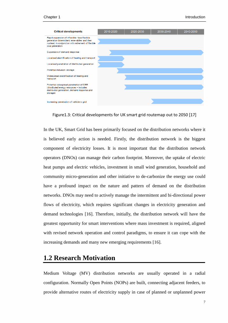
minimising costs to consumers. A “Smart Grid Routemap” was also published to
deliver this vision [16]. It emphasizes the potential role of the smart grid as a key
enabler to help UK power system accommodate a number of critical developments in
the next 40 years. The detailed developments with an illustrative timeline are given in
Figure 1.3 [17].
Chapter 1 Introduction
7
Figure1.3: Critical developments for UK smart grid routemap out to 2050 [17]
In the UK, Smart Grid has been primarily focused on the distribution networks where it
is believed early action is needed. Firstly, the distribution network is the biggest
component of electricity losses. It is most important that the distribution network
operators (DNOs) can manage their carbon footprint. Moreover, the uptake of electric
heat pumps and electric vehicles, investment in small wind generation, household and
community micro-generation and other initiative to de-carbonize the energy use could
have a profound impact on the nature and pattern of demand on the distribution
networks. DNOs may need to actively manage the intermittent and bi-directional power
flows of electricity, which requires significant changes in electricity generation and
demand technologies [16]. Therefore, initially, the distribution network will have the
greatest opportunity for smart interventions where mass investment is required, aligned
with revised network operation and control paradigms, to ensure it can cope with the
increasing demands and many new emerging requirements [16].
1.2 Research Motivation
Medium Voltage (MV) distribution networks are usually operated in a radial
configuration. Normally Open Points (NOPs) are built, connecting adjacent feeders, to
provide alternative routes of electricity supply in case of planned or unplanned power
Chapter 1 Introduction
8
outages. The unique benefit of this configuration is its inherent simplicity of operation
and protection. However, this needs to be reconsidered under the new circumstance.
With increasing penetration of intermittent renewables and growing electricity demand,
distribution networks are facing the challenge of increasing power flows through
existing networks. Although traditional network reinforcement is an option to deliver
the additional network capacity, their high-cost and time-consuming features make this
solution undesirable. Innovative solutions are therefore needed to increase the
utilization of existing assets dynamically and reroute the power flow through less
loaded circuits.
One way is to interconnect (or mesh) the conventional radial network, which enables
the power delivery through a less heavily loaded feeder and hence relieves the stress on
the heavily loaded feeders. Currently this configuration has been recognized by several
DNOs in their development plans [18], achieved by closing the NOPs. Benefits of a
closed loop network include balancing the loads between different feeders, improving
the voltage profiles, reducing power losses and improving the reliability. However, the
main problems of interconnection are:
The rise in fault current, which could lead to the malfunction of the existing
circuit breakers.
The need of more complicated and expensive protection schemes.
An alternative solution between the radial and the mesh operation is to have a flexible
mesh configuration. It is achieved by using a power electronic based device, named
Soft Open Point (SOP), to replace the NOP. Instead of simply opening/closing the NOP,
an SOP is able to provide the following functionalities:
Flexible control of active power exchange between connected feeders;
Flexible manipulation (absorbing and supplying) of reactive power on both
interface terminals;

Chapter 1 Introduction
9
Immediate fault isolation between interconnected feeders;
Small and controllable contributions to fault current;
Immediate post-fault supply restoration to support isolated loads on a feeder
through power transfer from the adjacent feeder.
Therefore, the SOP offers further flexibility to current distribution networks. For
network operation, it is envisioned to release capacity of existing feeders, enhance the
efficiency and service quality to customers. This thesis is motivated to investigate the
following three points, regarding the use of SOPs for MV distribution network
operation.
1.2.1 Control of an SOP
The SOP is a multi-functional power electronic device, and hence its control strategy
should be able to realize all the aforementioned functionalities. Previous studies (the
detailed discussion is in Section 2.3) mainly focused on the use of SOP under normal
network operating conditions, where the current-controlled strategy was used to
achieve independent control of real and reactive power. However, this
current-controlled strategy is not suitable to provide post-fault supply restoration
(another functionality of the SOP) because it may result in voltage and/or frequency
excursions that lead to either unacceptable operating conditions or instability. The
operating principle of an SOP therefore needs to be investigated under both normal and
abnormal network operating conditions.
1.2.2 Benefits analysis of using SOPs
It is urgently needed to quantify the benefits of SOPs for distribution network operation,
which provides confidence for using SOPs in distribution networks. SOPs are effective
in reducing power losses, balancing feeder loads, improving voltage profile, and
thereby increasing network loadability and DG connections. A number of studies (the

Chapter 1 Introduction
10
detailed discussion is in Section 2.3) can be found for these purposes. However, they
are mainly based on installing one or two SOP in a simple two-feeder network together
with the controller design and simulation. Methodologies for the benefit quantification,
i.e., steady state analysis of distribution networks with SOPs were not addressed and
the advantages of a more widespread use of these devices in distribution networks have
not been explored. In addition, distribution network reconfiguration has been
intensively researched. It could achieve similar objectives as the SOP. However, unlike
the SOP control, network reconfiguration is achieved by changing the network
topology: closing some NOPs while opening the same number of closed switches to
maintain a radial network structure. Extensive research has been conducted into
network reconfiguration (the detailed discussion is in Section 2.2.1) for feeder load
balancing, loss minimization and voltage profile improvement. It is needed to have a
comparison between using SOPs and network reconfiguration to enhance the operation
of a distribution network.
1.2.3 Distribution network voltage control with SOPs
Increasing DG capacity in the distribution network could cause the violation of voltage
limits. SOPs are able to assist voltage control through changing the real and reactive
power flow. Previous studies (detailed discussion is in Section 2.3) have reported the
potential of using SOPs for network voltage control. However, the voltage control
strategy considering the detailed operation of a SOP (determining the set points of the
SOP) has not been investigated. In addition, coordination with other network
controllable devices could achieve a better performance. There is a clear need to
develop a coordinated voltage control strategy, in which the SOP and other voltage
control devices are used together to achieve a better network voltage control.
Chapter 1 Introduction
11
1.3 Objectives and Contributions of this Thesis
The objectives and contributions of this work are outlined as:
Investigate the operating principle of an SOP using back-to-back VSCs under
both normal and abnormal network operating conditions.
Two control modes were developed for the operation of a back-to-back VSC
based SOP. The operating principle of the back-to-back VSC based SOP was
investigated under both normal and abnormal network operating conditions. The
performance of the SOP using two control modes has been analysed under
normal conditions, during a fault and post-fault supply restoration conditions.
Investigate the benefits of a MV distribution network with SOPs under normal
network operating conditions, focusing on feeder load balancing, power loss
minimization, and voltage profile improvement.
A steady state analysis framework was developed to quantify the benefits of
SOPs in MV distribution networks. The framework considers the network
reconfiguration and the combination of both SOP and network reconfiguration.
Investigate the use of the SOP for network voltage control and its coordination
with OLTC and DG units in an MV distribution network. The coordinated
voltage control strategy is able to maintain the network voltage while mitigating
DG active power curtailment, reducing the tap operations and the network
power losses.
A novel coordinated voltage control strategy was proposed considering the SOP,
the OLTC and multiple DG units. A distributed control framework was used,
considering each of the controllable devices as a local control agent. A

Chapter 1 Introduction
12
priority-based control was developed, achieving the specified objectives in
accordance with their prioritisation. Unlike centralised control strategies
(detailed discussion in Section 2.2.2), which requires communication links with
each network node and power flow solutions at each time step, this coordinated
voltage control strategy achieves a trade-off among objectives with fewer
communicational requirements and less computation burden.
1.4 Thesis Outline
The rest of this thesis is organized as follows:
Chapter two provides a literature review of challenges for distribution network
operation. Available network operation functions in facing the emerging challenges are
then introduced, with special attention paid to the network reconfiguration, coordinated
voltage control and those functions offered by using power electronic devices in
distribution networks. Last, the state-of-the-art of SOPs, including the benefits, possible
device types and previous studies are presented.
Chapter three describes two control modes for the operation of a back-to-back
VSC based SOP. The operating principle and performance of the back-to-back VSC
based SOP using these two control modes were analysed under both normal and
abnormal network operating conditions.
Chapter four describes a steady-state analysis framework to quantify the
operational benefits of a distribution network with SOPs. A generic model of an SOP
for steady-state analysis was developed. Based upon it, an improved Powell’s direct set
method was developed to obtain the optimal SOP operation. Distribution network
reconfiguration algorithms, with and without SOPs, were developed and used to
identify the benefits of using SOPs. Case studies have been conducted with promising

Chapter 1 Introduction
13
results obtained for using SOPs in MV distribution networks.
Chapter five describes a novel coordinated voltage control strategy, considering
SOPs, OLTC and DG units, to maintain network voltages while mitigating DG active
power curtailment, reducing the tap operations and the network power losses. A
distributed based voltage control framework was developed which uses a simplified
voltage profile estimation method. Followed by an analysis of using SOP for
distribution network voltage control, a priority-based coordination, using the proposed
voltage control framework, was developed to achieve a trade-off among the objectives.
The effectiveness of the proposed coordinated control strategy was verified under
various loading and DG penetration conditions.
Chapter six presents the conclusions drawn, main findings and recommendations
for future work.

Chapter 2 Literature Review
14
Literature Review
HIS chapter presents a literature review on the challenges for
distribution network operation, the network operation functions and
the state-of-the-art of the SOP studies.
T
Chapter 2

Chapter 2 Literature Review
15
2.1 Challenges for Distribution Network Operation
Since the Carbon Emission Reduction Target (CERT) was introduced into the electric
industry, electric power distribution networks have undergone dramatic changes. In this
CERT context, distribution networks should not only be able to deliver electricity to
customers with acceptable reliability and quality standards, but also to fulfil the tasks, such
as accommodating increasing renewable energy sources and meeting the sustained high
level of demand growth resulting from the electrified heating and transport, etc. These
requirements impose great challenges to distribution networks, in particular in the
operation perspective.
2.1.1 Aging Assets and Lack of Circuit Capacity
In many parts of the world (e.g., the USA and most European countries), the electric
power system expanded rapidly in 1950s and 1960s [19]. The distribution equipment
and cables installed then are now beyond its design life and in need of replacement. The
capital costs of the like-for-like replacements will be very high [19]. The need to
refurbish the transmission and distribution circuits is an obvious opportunity to
innovate with new designs and operating practices. In addition, the introduction of
intermittent DGs can increase the use of tap-changing devices (e.g., OLTC and
switched capacitor banks) and therefore accelerate failure of the device [20]. A smarter
operation is therefore needed to make effective use of existing assets and mitigate the
wear and tear.
In many countries, constructing new overhead lines, needed to meet the load growth
and to connect renewable DGs, has been delayed for up to 10 years due to the
difficulties in obtaining rights-of-way and environmental permissions [19]. Therefore,
some of the existing distribution line circuits are operating near their capacity, limiting
DG integration and demand growth. This calls for intelligent methods, instead of
traditional network reinforcement, to increase the power transfer capacity of circuits

Chapter 2 Literature Review
16
dynamically and reroute the power flows through less loaded circuits.
2.1.2 Operational Constraints
Distribution networks have to operate within prescribed constraints in order to ensure
secure electricity delivery. These constraints include [21]: voltage constraints, thermal
constraints, frequency and short-circuit constraints, etc.
With the introduction of DGs and the continuous growth of demand, most distribution
networks are experiencing constraint breaches. The large-scale integration of DGs can
cause over-voltages at times of light load, and the demand growth can give rise to local
low voltages. Hence, adequate voltage management requires a coordinated operation of
the DGs, on-load tap changers and other equipment (e.g., voltage regulators and
capacitor banks). Due to the local reverse power flow brought by the DGs, aligned with
the increased demand, thermal limits of the existing transmission and distribution
equipment and lines can be exceeded. Thus dynamic ratings that can increase circuit
capacity in real-time are needed to address the thermal overloading. Some DG plants
use directly connected rotating machines, for example, old wind turbines and small
hydro turbines use induction generators while, large hydro turbines use synchronous
generators [22]. The connection of these generators and new spinning loads can cause
the maximum fault current to exceed the fault level rating of the distribution network.
Thus effective fault current limiting technologies or services are required to maintain
safe operation of the power system.
Therefore, distribution network operation has to be robust and flexible to address the
constraint problems that are caused by the quantity, geography and intermittency of the
DG integration as well as the new forms of load. Otherwise, traditional expensive
network reinforcement has to be carried out.

Chapter 2 Literature Review
17
2.1.3 Reliability and Efficiency of Supply
Morden society has increasing critical loads connected and power blackouts could
result in enormous monetary loss and society chaos [23]. In the coming decades, the
proportion of intermittent renewable generation in the energy mix will get higher,
lowering the overall predictability of the electricity supply. In the meantime, the
electricity capacity margin is reducing, which increases the risks to security of supply.
To meet the requirement of the Government’s reliability standard, UK’s utilities had
defined customer interruptions (CIs) and customer minutes lost (CMLs) as the indicator
of each DNO’s performance [24]. This calls for effective restoration strategies and
other post-fault measures to retain or return the supply after the (inevitable) faults in the
distribution networks.
Electrical power losses are an inevitable consequence of transferring electricity across
distribution networks and they have significant environmental and financial impact on
customers. For instance, the energy losses from the electricity distribution networks
contribute to approximately 1.5 % of Great Britain’s greenhouse gas emissions [25].
Moreover, present distribution networks usually have power losses in the range of 3% -
9% and this accounts for 80% of the total power losses in combined transmission and
distribution networks [24]. Higher losses (dominated by the ohmic loss: I2R terms)
would be expected in 2030 due to the anticipated more heavily assets use [24]. All
these losses are eventually paid for by customers and need to be mitigated. To
encourage an efficient level of losses in distribution networks, Office for gas and
electricity Market (OFGEM) has launched a losses incentive mechanism to be a part of
their network price control since 2015 [26]. An improved operating efficiency is
therefore needed for minimum energy losses.

Chapter 2 Literature Review
18
2.2 Network Operation Functions
As discussed in the previous section, distribution networks need better control and
supervision of distribution network facilities to support their operation in facing the
emerging challenges.
Traditionally, there are well established operation functions available that enable
control and supervision of distribution network facilities for desired network
performance. Examples include the network reconfiguration, voltage and reactive
power control, protection relay coordination and outage management, etc.
At present, the emergence of smart grid concept is a radical reappraisal of the functions
of distribution networks. In response to the smart grid initiatives, various new
technologies and applications are being introduced into distribution networks, such as
the integration of distributed energy resources, active control of demand load and the
progress of using distribution-level power electronics. These new technologies and
applications are able to support network operation neither by adding to the
effectiveness of existing operation functions (e.g., through a coordinated operation) or
by offering new functions to the distribution network.
This thesis focused on the enhancement of distribution network operation through the
use of power electronic based equipment - SOP - as well as its operation comparing and
coordinating with traditional network reconfiguration and network voltage control. As
background to the research that has been carried out, network reconfigurations,
coordinated voltage control and the operation functions that can be offered by using
power electronic devices in distribution networks will be introduced in subsequence
sections.

Chapter 2 Literature Review
19
2.2.1 Network Reconfiguration
Distribution networks are normally designed as meshed networks but are operated in a
radial manner with normally open points [27]. Network configurations can be changed
during the operation by changing the open/close status of switchgears, manually or
automatically [27]. Figure 2.1 gives an example of network reconfiguration, which is
based on a three-feeder network with three NOPs (dash lines). The configuration of the
network is changed by closing NOPs 15 and 26 while opening closed switches 12 and
13.
(a) (b)
Figure 2.1: Three-feeder example network: (a) before network reconfiguration; (b)
after network reconfiguration [27]
The main objectives of network reconfiguration include [19, 28]:
1. Supply restoration:This optimally restores de-energized customers through
alternative sources in the case of planned and unplanned power outages.
2. Load balancing among substation transformers or different feeders and
equalising the voltages.
3. Active power loss minimization at a given time or energy loss minimization
during a period.
Chapter 2 Literature Review
20
The methods used to solve the above network reconfiguration problems include those
based on practical experience and optimization techniques. The methods based on
optimization techniques determine the optimal network configuration by solving a
complicated combinatorial, non-differentiable constrained optimization problem [29].
Possible solutions include mathematical algorithms [27, 30], computational
intelligent-based algorithms (for example, generic algorithm, simulated-annealing,
fuzzy logic) [31-33], and hybrid algorithms which combine two or more above
algorithms [34, 35].
Network reconfiguration and its significant benefits have been reported in the past
decades. However, practical applications of automatic network reconfiguration is
presently very limited due to excessive costs of remotely-controlled switchgear,
associated ICT infrastructures and maintenance of hardware/software (e.g., excessive
wear and tear of switches) [36, 37]. The protection coordination requirement for the
reconfigurable network is also a hurdle [38].
It is possible to use SOPs to achieve the same aforementioned benefits (objectives)
offered by network reconfiguration. In the meantime, changes of network topology and
protection coordination are no longer needed when using the SOP. In the study reported
in Chapter 4, the potential and benefits of using SOP, compared with traditional
network reconfiguration, was discussed in further detail.
2.2.2 Coordinated Voltage Control
Voltage control refers to the technique of using available voltage control equipment to
maintain acceptable voltage levels at all points in the distribution network under all
loading conditions [39]. As discussed in Section 2.1, it is one of the most significant
issues that limits DG penetration in distribution networks. When DGs units are
connected to a distribution network, they can significantly change the network voltage
profile and interfere with conventional local control strategies of the transformer

Chapter 2 Literature Review
21
tap-changers, line voltage regulators and shunt capacitors (which are designed based on
the assumption of unidirectional power flow [40]). This interference leads to [41]: 1)
unexpected over- and under-voltage, 2) increase in power losses and 3) excessive wear
and tear of voltage control devices.
In these circumstances, a coordinated operation of the voltage control devices is needed
to provide adequate voltage management, meanwhile, eliminating the aforementioned
problems. In the literature, numerous control devices has been conducted to support
voltage control. Examples include [42-45]: on-load and off-load transformer
tap-changers, line voltage regulators and switched capacitor banks, energy storage,
power electronic devices and the control of DG.
These control devices are the key factors to realize the coordinated voltage control in
distribution networks. However, the first milestone is to find a most effective control
strategy to achieve the coordination among the control devices. In the literature,
numerous voltage control strategies have been proposed to achieve a proper
coordination. According to the control structure and communication links, they can be
categorized as [46]:
i) Localized coordination: with no communication links,
ii) Centralized coordination: with a wide range of communication links,
iii) Distributed coordination: with a few communication links among control
devices.
Localized coordination
Localized coordination does not require communication links. Control devices
determine their operating set points based on local signals [39]. The coordination
between the localized control actions can be achieved based on the time delay operation
[40]. Alternatively, the local control strategies for DG units can be modified to mitigate

Chapter 2 Literature Review
22
their impacts on the voltage profile, without modifying conventional local control
strategies. For example, the authors in [47] proposed a decentralized reactive power
control approach for the DG units, which absorbs reactive power to compensate the
effect of voltage rise caused by active power injection. Therefore, the convention local
control strategy is not affected by the reverser power flow.
The localized coordination approaches are reliable and scalable due to their
independency and simplicity of control structure. However, their control performances
are not optimal. Examples include: 1) the high stress on the control devices is not
relieved, 2) the energy capture from DG units is not maximized, and 3) the feeder
power losses may increase.
Centralised coordination
Centralized coordination is a fully-coordinated control approach that calculates the
optimal operating set points for all available controllable devices and delivers the best
performance possible by solving a multi-objective optimization problem [48]. It is
usually achieved based on a distribution management system (DMS) to receive
measurements of the distribution network (e.g., voltage, power flow, and equipment
status), and, then, to estimate the network status before dispatching control devices
using state estimation technologies [49].
Figure 2.2 shows an example of the cascaded control architecture for centralized
coordination. The distribution management system solves the optimization problem by
either following different objectives at different times or considering conflicting
objectives together in a weighted manner [50-54]. The DMS then dispatches the control
devices accordingly via the supervisory control and data acquisition (SCADA) systems.
The main downsides to the centralized coordination include [49, 55]: 1) The extensive
investment in sensors and communication links; 2) The requirement for the accuracy of

Chapter 2 Literature Review
23
the state estimator; 3) The use of power flow and optimization solution at each time
step, which might cause a large computation burden and numerical convergence issues
when X/R ratio is low; 4) The undesirable properties with respect to scalability and
reliability (fragile to single point of failure).
Figure 2.2: Cascaded control architecture for centralized coordination [48]
Distributed coordination
Distributed coordination has been proposed recently to tackle the drawbacks of
centralized and localised coordination [55]. It is usually accomplished by using a
multi-agent framework. Each agent in the framework is an intelligent entity that can
perceive its environment, create an action according to its own decision-making and
communicate with other agents to achieve a common goal [46]. For voltage control
problems, each control device is considered as an local control agent and communicates
with other agents for improved control performance [46].
Compared with the centralized coordination, distributed coordination can reduce the
communication requirements and computation burden as well as avoid the reliability
issue (for example, single point of failure) because the dispatching is implemented in a

Chapter 2 Literature Review
24
distributed manner, i.e., the original problem is decomposed into smaller sub-problems
and each is assigned to a particular agent [56]. In addition, the implementation of
centralized coordination becomes difficult with the increase of uncertainties due to DG
integration and the efforts to achieve a “plug and play” property. Distributed
coordination is expected to deal or at least relieve these issues [56]. In this thesis, the
distributed coordination was employed to provide coordinated voltage control in an
active distribution network with SOPs.
Numerous efforts have previously been made to achieve distributed coordination for
network voltage control using the multi-agent framework [41, 46, 55-57]. In [56], a
multi-agent reactive power dispatching scheme was proposed for voltage support of
DG units in a single feeder. But the utility voltage control devices (for example, OLTC,
shunt capacitors) were not considered. The authors in [57] proposed a coordinated
voltage control for the OLTC control, where the remote terminal units were treated as
local control agents and provide distributed state estimation. However, the OLTC was
assumed as the only control devices. In [41] and [55], multi-agent frameworks were
proposed for coordinated voltage control between both DG units and utility control
devices. Figure 2.3 shows an example of the coordination among three control agents
via two ways communication [41]. All three control agents have a common objective
and each agent also has its own objective (see the circles). The control agent can take
local measurements, make control decisions and negotiate with other agents when there
is a need. In these studies, the control performances highly depend on their control
design since the control optimality tends to be degenerated by the negotiation process
among agents.
Another coordinated control strategy using a multi-agent framework was proposed in
[46] to achieve both autonomy and optimal control. The use of “blackboard” memory
data combined with the multi-agent framework can eliminate unnecessary negotiation
process among agents and minimize data communications. However, the extensive

Chapter 2 Literature Review
25
investment on sensors, the computation burden and the convergence issues due to
running power flow were not addressed in this study.
Figure 2.3: Coordination among three control agents via two ways communication [41]
In this thesis reported in Chapter 5, based on the proposed distributed coordination, a
simplified voltage estimation method was used to reduce the number of sensors in the
network. In addition, a coordination method was applied on the control agents (SOP,
OLTC and DGs), which can eliminate unnecessary negotiation process among the
agents and provide improved control performance without running power flow.
2.2.3 Operation Functions Offered by Power Electronic devices
Power electronics, in forms of the high-voltage DC transmission system (HVDC) and
flexible AC transmission systems (FACTS), has played a visible and key role in
power-gird control for over 60 years, mainly on the transmission network for bulk
power transfer [58]. The use of power electronics at the distribution network level has
been much more limited. At present, under the smart grid concept, visibility,
controllability, and flexibility will be essential features throughout the future
distribution network where power electronics can play a key role [19]. Several DNOs
in the UK have already initiated to offer power electronics solutions to address their

Chapter 2 Literature Review
26
network issues [59-61] and, hence, delay or eliminate the need of traditional network
reinforcement. Further literature on the advantages of power electronic solutions over
traditional network reinforcement is available in [18].
A wide variety of network operation functions can be offered by using power electronic
devices in distribution networks. Examples include voltage control, phase rebalancing,
active power filtering, fault current limiting and power flow control, etc.
Power electronics can support distribution network voltage control in forms of power
electronic transformers [62], transformers with electronic tap changers [63] and
reactive power compensation. Power electronic transformers and transformers with
electronic tap changers can be installed in place of classical transformers, providing the
competitive advantages of enabling fast and smooth voltage regulation as well as little
wear and tear. The reactive power compensation, such as using the STATCOM [64],
dynamic voltage restorer (DVR) [65] and SOP [61], can tackle the voltage problem
either at the substation, path-way along the feeder or at the point-of-load.
Phase imbalance, as a result of differences in consumption patterns of consumers, can
cause higher conduction losses and lower network utilization. It is also considered as a
major cause of capacity limitation [66]. Power electronic devices that contain a
common DG bus, such as the unified power quality conditioner, DVR, STATCOM and
SOP, allow exchange of instantaneous power between the phases and, hence, can be
used to rebalance current flow on a feeder.
Active power filters for harmonic elimination and power quality improvement have
been applied within customer premises but not as network elements compensating a
group of consumers [18]. In recent years, the need for filtering in networks with power
electronic compensation has been recognized by DNOs, such as filtering in the
locations with a high penetration of PV [18].

Chapter 2 Literature Review
27
Power flow control are traditionally achieved through network reconfiguration with
existing switchgear (discussed in Section 2.2.1), aiming to increase the power transfer
capacity of circuits dynamically and reroute the power flows through less loaded
circuits. At present, an alternative solution, that makes use of power electronics in the
form of SOP to facilitate power flow in a dynamic and continuous manner, is attracting
the interest of the DNOs. A Low Carbon Networks Fund (LCFN) project has already
initiated to install the SOP in UK’s distribution network to verify its effectiveness [61].
This thesis focuses on the new power electronics application. Details on the
introduction of SOP benefits, types and previous work are presented in the following
section.
2.3 Soft Open Points
2.3.1 Benefits of Soft Open Points
As shown in Figure 2.4, SOPs are multi-functional power electronic devices (discussed
in Section 1.2) installed in place of the NOPs in distribution networks. They are also
referred to as ‘loop power flow controllers’, ‘series controllers’ and ‘DC links’ in some
literatures.
Figure 2.4: Simple distribution network: option A representing a NOP connection
and B representing an SOP [67]

Chapter 2 Literature Review
28
The most significant advantageous provided by these power electronic devices,
compared with mechanical switches, are
The power flow between the connected feeders can be regulated in a continuous
and dynamic manner.
The reactive power is able to be independently injected or absorbed at both
interface terminals. Therefore, SOP can be used for dynamic voltage support.
The SOP can be used to improve the power quality of the distribution networks
[68], such as mitigating voltage imbalance, sags, flickers, and low-order
harmonics, etc.
The SOP can be used to connect any feeders regardless of the angular or rated
voltage difference between them, particularly when the feeders are supplied by
different substations. This is not possible with the mechanical switches.
The short-circuit currents on the radial feeders (without SOPs) are not changed
with the use of SOPs, owning to the capability of instantaneous fault current
control. This indicates that this intervention would not require modifications of
existing network protection assumptions or upgrades of protection devices (this
is usually the case for a close-loop operation). [69]
2.3.2 Types of Soft Open Points
The functionalities of an SOP were descripted in Section 1.2. Possible SOP types,
enable to realize these defining functionalities, include:
Back-to-back VSCs
Multi-terminal VSCs
Unified power flow controller (UPFC)
An overview of the topologies of these types of SOPs is shown in Figure 2.5. Each is

Chapter 2 Literature Review
29
made from an arrangement of VSCs with varying rating and quantity. The VSC is
suitable for SOPs due to: 1) the freedom to operate with any combination of active and
reactive power, 2) the ability to limit (or control) fault current and 3) the possibility to
supply isolated areas of a network or even provide the black-start ability.
Figure 2.5: Topologies of different types of SOPs [70]
Back-to-back VSCs
This thesis focused on the back-to-back VSC based SOP. It consists of two VSCs
connecting via a common DC link to form an asynchronous AC/AC conversion device.
Coupling transformers are usually equipped, interfacing each VSC with the connected
feeder. However, transformerless topologies are possible [71], which reduces the size
and weight of the device. This arrangement allows active power exchange between the
AC front ends as well as independent reactive power manipulation at each interface
terminal.
Under abnormal network conditions, the fault on one feeder can be isolated from the
other feeder by the DC link. The fault current on the faulted side interfacing VSC can
also be limited (and controllable) by appropriate control strategy [68]. Post-fault
restoration is achievable, supplying the isolated loads on one feeder by power transfer
from the adjacent feeder via the VSCs [68].

Chapter 2 Literature Review
30
Multi-terminal VSCs
The multi-terminal VSC based SOP is an extension of the back-to-back VSC based
SOP, in which additional VSCs are connected to a common DC-link. The number of
VSCs associated with a multi-terminal VSC based SOP is defined as 3 or greater. The
same features discussed for the back-to-back VSC based SOP are applicable to the
multi-terminal VSC based SOP.
Unified power flow controller (UPFC)
The UPFC based SOPs, also known as shunt-series VSCs, consists of two VSCs with a
common DC link. Unlike the configuration of the aforementioned two types, one VSC
in UPFC is connected in series and the other is connected in shunt with the
interconnected feeders. The series connected VSC injects a series voltage with
controllable magnitude and phase angle, thereby controlling the power flows between
interconnected feeders [72]. The shunt connected VSC supplies the active power
demanded by the series VSC through the DC link. It can also provide reactive power
manipulation independent of the operation of the series connected VSC.
The primary advantage of the UPFC based SOPs, compared with the aforementioned
two types, is the potential to induce power flows greater than VSC rating (for example,
10 MVA transferred using 1 MVA VSCs). However, this ability is determined not only
by the device ratings themselves, but also by the network topology, constraints, and
operating point as well as the device placement [70]. An inherent drawback to the
UPFC is the fact that the feeders connected with a UPFC are not isolated by a DC-link,
and, hence, disturbances or faults on one connected feeder will affect the other unless a
control strategy is developed to reject or compensate for disturbances. The
instantaneous fault current limitation (or blocking) is possible [73], at the cost of higher
device ratings. The interconnection is also not asynchronous and therefore the two
electrical network connected via a UPFC based SOP must be synchronous.

Chapter 2 Literature Review
31
2.3.3 Previous Soft Open Points Studies
Previous work on SOPs is discussed with the research gaps identified in terms of the
control strategy, benefits analysis and their use for distribution network voltage control.
Control strategy
The control strategy of an SOP has been reported early in 2006 [71]. A
current-controlled strategy was developed for the operation of a back-to-back VSC
based SOP. In this control strategy, direct-quadrature (d-q) current components were
used for each VSC to provide control of instantaneous active and reactive power
exchange between the VSC and the AC network. The effectiveness of the control
strategy for instantaneous power flow regulation has been verified by a factory test
using 6.6kV 1MVA transformerless back-to-back VSCs. But the performance of this
control strategy under abnormal network conditions, i.e., during a fault and post-fault
supply restoration, was not investigated.
In [74], the same current-controlled strategy was applied to a multi-terminal VSCs
based SOP and validated in an experimental way. The transient performance of the
control strategy during a three-phase short-circuit fault was evaluated. This current
limiting capability has been demonstrated important to 1) protect VSCs from
over-currents and 2) limit fault current and therefore maintain the same short circuit
current as the radial network operation (without VSCs). Nevertheless, the operation of
the SOP for post-fault supply restoration was not considered.
When the SOP provides post-fault supply restoration to isolated loads, the frequency
and voltage are not dictated from the grid. Hence, the aforementioned control strategy
is not desirable because it may cause voltage and/or frequency excursions that can lead
to either unacceptable operating conditions or instability [75]. The operating principle
of an SOP under both normal and abnormal network operating conditions was not
found in previous literatures and need to be investigated.

Chapter 2 Literature Review
32
Benefits analysis
The benefits of using SOPs in distribution networks have previously been reported for
different objectives, such as: loss minimization [76-78], feeder load balancing [36, 37]
and maximisation of network loadability and DG penetration [69, 79, 80]. The authors
in [69] developed an optimization framework to compare the benefits of using DC links
(which are also SOPs) with conventional network reinforcement measures. Using the
framework, a thorough assessment of the most promising SOP type was reported in
[79]. The benefits of the back-to-back VSC based SOP, UPFC based SOP and a series
VSC were analysed and compared in terms of their capability to maximise DG
penetration in distribution networks.
In these literatures, operational benefits of using SOPs were studied mainly based on
two or three feeders connected by an SOP. Methodologies for benefit quantification and
the advantages of more widespread use of SOPs in distribution networks have not been
explored.
On the other hand, it is possible to maximise the benefits of an SOP by combining with
traditional network reconfiguration (discussed in Section 2.2.1). An SOP is only able to
regulate the power flow of its own connected feeders. Using network reconfiguration
can change the feeders that are connected to the SOP dynamically and, hence, can
benefit the whole network. The combination of network reconfiguration and SOP
control and its benefits are discussed in further detail in Chapter 4.
Distribution network voltage control
The potential to use SOPs for distribution network voltage control has been reported
[67] [81] by changing active and reactive power flows on the connected feeders.
In [81], the minimum voltage deviation among multiple feeders was achieved by using
a multi-terminal VSCs based SOP. The effectiveness of using an SOP to mitigate

Chapter 2 Literature Review
33
voltage deviation was compared with that using a close-loop operation. Similar
performance was observed while the later one requires more complicated protection
system. However, in this study, the reactive power control ability of the SOP was not
considered.
In [67], the use of SOPs, controlling both active and reactive power flow, has been
proposed for network voltage control and, ultimately, higher DG penetration in
distribution networks. A comparative analysis was conducted between using SOPs and
conventional voltage control options (for example, OLTC). However, the operation of
the SOP (set points of active and reactive power) was determined by merely satisfying
constraints. Well-established voltage control strategies including suitable operation
mechanisms of the SOP were not elaborated in this study. In addition, the coordination
of SOPs and other available voltage control devices for improved control performance
has not been investigated in previous work.
2.4 Summary
Challenges for distribution network operation were summarized. The network operation
functions that enable to deal with emerging challenges were then introduced, with
special attention paid to the network reconfiguration, coordinated voltage control and
those functions offered by using power electronics in distribution network level. The
power electronic applications can offer a variety of operation functions and, hence, will
play a key role to enable visibility, controllability, flexibility features throughout the
future distribution networks.
SOP is a power electronic application in distribution networks. The possible layout of
SOP and its benefits were introduced. In addition, a review of the state-of-the-art of the
SOP studies was presented and followed by identifying the corresponding research
gaps.

Chapter 2 Literature Review
34
The current-controlled strategy has been reported for SOP operation to achieve the
defining functionalities. However, this control strategy is not suitable for post-fault
supply restoration (which is another key functionality of SOP). The operating principle
of an SOP under both normal and abnormal network operating conditions is yet to be
explored. Therefore, in this study, operating principle of a back-to-back VSC based
SOP was investigated under normal conditions, during a fault and post-fault supply
restoration (discussed in Chapter 3).
The benefits that an SOP can provide have been identified. However, methodologies for
benefit quantification and the advantages of more widespread use of SOPs in
distribution networks were not explored. In addition, using SOP control could achieve
the same objectives as traditional network reconfiguration, and a combination of both
SOP control and network reconfiguration could maximize the benefits of an SOP as
well as benefit the whole network. These issues have not been explored in previous
studies. Therefore, in this study, the operational benefits of using SOPs, with and
without considering network reconfiguration, were quantified and reported in Chapter
4.
Distribution network voltage control can be achieved by using SOP through both active
and reactive power flow control. However, research conducted on suitable operation
mechanism of SOPs for distribution network voltage control and the coordination with
existing voltage control devices was not found. Therefore, in this study, a coordinated
voltage control strategy in active MV distribution networks with SOPs was investigated
(discussed in Chapter 5), which is based on the distributed coordination.

Chapter 3 Control of a Back-to-Back VSC based SOP
35
Control of a Back-to-Back
VSC based SOP
HIS chapter investigates the operating principle of a back-to-back VSC
based SOP under both normal and abnormal network operating
conditions
Chapter 3
T

Chapter 3 Control of a Back-to-Back VSC based SOP
36
3.1 Introduction
In this chapter, the circuit topology of back-to-back VSCs and its suitability for the role
of an SOP is presented. Two control modes were developed for the operation of a
back-to-back VSC based SOP. The operating principle of the back-to-back VSC based
SOP with these two control modes was investigated under both normal and abnormal
network operating conditions.
Studies on a two-feeder MV distribution network showed the performance of the SOP
under different network operating conditions: normal, during a fault and post-fault
supply restoration. During the change of network operating conditions, a mode switch
method was used to achieve the transition between the control modes. The role and
importance of soft cold load pickup and voltage synchronisation processes, essential for
a smooth transition during the switching of control modes, were also investigated.
3.2 Back-to-Back VSC based SOP
Figure 3.1a shows a two-feeder distribution network interconnected with a
back-to-back VSC based SOP. Two VSCs are located between the feeder endpoints and
connected via a common DC link. The main circuit topology of the back-to-back VSCs
is shown in Figure 3.1b. It consists of a DC capacitor to provide an energy buffer and
reduce DC side voltage ripple, two two-level three-phase insulated gate bipolar
transistor (IGBT)-based VSCs to generate voltage waveforms using pulse width
modulation (PWM), and two series inductances [82]. These inductances provide
high-frequency harmonic attenuation, limit the rate of rise of short circuit current, and
facilitate control of power flow.

Chapter 3 Control of a Back-to-Back VSC based SOP
37
Feeder I
Real
power
Reactive
power
SO
P
Feeder II
MV distribution network
Reactive
power
(a)
+
-
Lf
VSC2
CLf
Lf
Lf
VSC1
Lf
Lf
(b)
Figure 3.1: (a) Basic configuration of a distribution network with an SOP; (b) Main
circuit topology of the back-to-back VSC based SOP.
The back-to-back VSCs are suitable for SOP operation due to the following
characteristics:
Flexible active and reactive power control
Both VSCs build their own voltage waveforms with desired amplitude and phase angle.
This allows a full control of active power flowing through the DC link as well as
independent reactive power supply or absorption at both interface terminals. This
controllability enables SOP operation for normal network operating conditions, which
includes feeder load balancing, power loss reduction and voltage profile improvement.

Chapter 3 Control of a Back-to-Back VSC based SOP
38
Instantaneous and independent voltage control
The voltage waveform built by the VSCs can be controlled dynamically within
milliseconds thus enabling transient control, e.g. dynamic Volt/VAR control and power
oscillation damping [83]. In addition, the VSC can build its own voltage without the
need of an active source at the receiving end. Hence cold load pick up for supply
restoration is achievable using such device.
Disturbance and fault isolation
Network disturbances and faults on one connected feeder can be isolated from the other
side by the back-to-back VSCs since transient overvoltage and overcurrent are able to
be limited by the control scheme [84].
3.3 Control Modes of the Back-to-Back VSC based
SOP
Two control modes were developed to operate the back-to-back VSC based SOP under
both normal and abnormal network operating conditions. The power flow control mode
was used to 1) regulate both active and reactive power flow on the connected feeders
under normal network operating conditions and 2) isolate fault between the
interconnected feeders when a fault occurs on one feeder. The supply restoration mode
was used under post-fault supply restoration conditions to provide power supply for the
isolated loads on one feeder through the other feeder.
3.3.1 Power Flow Control Mode
A dual closed-loop current-controlled strategy [85] was used to operate SOP for the
control of the feeder power flow under normal network operating conditions.
Current-controlled strategy is advantageous because: 1) it provides de-coupled control
of active and reactive power components; and 2) it inherently limits the VSC current

Chapter 3 Control of a Back-to-Back VSC based SOP
39
during network faults.
Figure 3.2 presents the overall control structure. The outer power control loop, the inner
current control loop and the PLL are the three main components. In the outer power
control loop (Figure 3.2a), one of the VSCs operates with the P-Q control scheme
where the active and reactive power errors are transformed into the reference d-q
current components, 𝑖𝑑∗ and 𝑖𝑞
∗ through the proportional-integral (PI) controllers.
Superscript asterisk denotes the reference values. The other VSC operates with the
𝑉𝑑𝑐 − 𝑄 control scheme maintaining a constant DC side voltage for a stable and
balanced active power flowing through the DC link. Dynamic limiters for 𝑖𝑑∗ and 𝑖𝑞
∗
are inserted to enable overcurrent limiting during network faults and disturbances. In
the inner current control loop (Figure 3.2b), the reference VSC d-q voltage, 𝑉𝑑𝑚 and
𝑉𝑞𝑚 are determined through the PI controllers considering the d-q current errors. The
voltage feed-forward and current feed-back compensations are used to get a good
dynamic response [86]. After transforming 𝑉𝑑𝑚 and 𝑉𝑞𝑚 into the VSC terminal
voltage by the inverse of Park’s transformation [87], the gate signals for the IGBTs are
obtained through the PWM. The PLL is important for the connection of VSCs to the
AC network in order to synchronize the phase of the output VSC voltage with the AC
network voltage. A PLL control topology based on the pq theory was used [88], as
shown in Figure 3.2c. By using the sum of the products of the feedback signals, 𝑓𝛼
and 𝑓𝛽 , and input 𝛼 − 𝛽 voltages (from Clark’s transformation [87] of the phase
voltages), the variation of the angular frequency ∆𝜔 is calculated as:
∆𝜔 = 𝑉𝛼 ∙ 𝑓𝛽 + 𝑉𝛽 ∙ 𝑓𝛼 (3-1)
The PLL output angle 𝜃 is then obtained using a PI-controller, a feedback of the base
angular frequency 𝜔𝑏 and an integrator.

Chapter 3 Control of a Back-to-Back VSC based SOP
40
+- PI
+- PI+- PIP
P*
Q
vdc
vdc*
iqmax
0
idmax
0
idmax
0
+- PI
Q*
Q
iqmax
0
id*
iq*
id*
iq*
Q*
Vdc -Q schemeP -Q scheme Power control loop
(a)
+PI+- +
+
-+
-+PI
wL
wLabc
dq
PWM
id
iq
vq
vd
id*
iq*
vqm
vdm vam vbm vcm
+
Gate signals
abc
dq
θ
θ
abc
dq
vd vq
Current control loop
vga
vgb vgc
iga
igb
igc
(b)
X
X
-sin
cos
θ
abc
ɑβ
PLL
w PI 1s
fɑ
fβ
∑ ∑
wb
w
vga vgb vgc
vɑ
vβ
(c)
Figure 3.2: Control block diagram of the SOP for power flow control mode: (a) outer
power control loop; (b) inner current control loop; (c) PLL controller
3.3.2 Supply Restoration Mode
When loads connected to one VSC of an SOP are isolated, the frequency and voltage of
this VSC are no longer dictated by the grid. Using the previous current control strategy
will cause voltage and/or frequency excursions and hence may lead to unacceptable
operating conditions [75].
In such a case, the interface VSC (connected to the isolated loads) changes to act as a

Chapter 3 Control of a Back-to-Back VSC based SOP
41
voltage source in order to provide a desired load voltage with stable frequency. The
other VSC still acts as a current source operating with the 𝑉𝑑𝑐 − 𝑄 control scheme.
Figure 3.3 shows the block diagram of the voltage and frequency control strategy for
the interface VSC. For voltage control, the VSC output voltage is controlled directly in
the d-q synchronous frame by holding 𝑉𝑞∗ to zero and controlling 𝑉𝑑
∗ as:
𝑉𝑑∗ = √2/3 ∙ 𝑉𝑟𝑚𝑠
∗ (3-2)
where 𝑉𝑟𝑚𝑠∗ is the desired nominal line to line rms voltage of the isolated loads.
√2/3 is included because Park’s transformation is based on the peak value of the
phase voltage. The output VSC voltage is regulated by closed loop control and
generated through the PWM scheme. For frequency control, a stable voltage frequency
is generated by using the PLL. The input phase voltages of the PLL are assigned by
transforming the reference d-q voltages, 𝑉𝑑∗ and 𝑉𝑞
∗ ( 𝑉𝑞∗ =0) through Clarke’s
transformation. Thus, ∆𝜔, as shown in Figure 3.2c, is calculated as:
∆𝜔 = 𝑉𝛼 ∙ 𝑓𝛽 + 𝑉𝛽 ∙ 𝑓𝛼 = 𝑉𝑑∗ ∙ cos 𝜃 ∙ (− sin 𝜃) + 𝑉𝑑
∗ ∙ sin 𝜃 ∙ cos 𝜃 = 0 (3-3)
Since ∆𝜔 remains zero, the phase angle 𝜃 with a fix frequency of 50 Hz can be
generated by integrating only the base angular frequency 𝜔𝑏 = 2𝜋 × 50 Hz.
+- abc
dq
PWM
Vrms*
PI
PIvam
vbm
vcm
+-
0
√2/3
abc
dq
abc
PLL
vla vlb vlc
θ
dq
vd*
vq*
vq
vd
vdm
vqm
Gate signals
θ
θ
θ
Figure 3.3: Control block diagram of the interface VSC for supply restoration control
mode

Chapter 3 Control of a Back-to-Back VSC based SOP
42
3.4 SOP Operation in MV Distribution Networks
The operating principle and performance of the back-to-back VSC based SOP under
different network operating conditions was analysed using a test system shown in
Figure 3.4. It consists of two MV feeders with constant impedance loads extracted from
an IEEE 33-bus distribution network [20] and a back-to-back VSC based SOP placed
between the feeders. This test system was modelled in EMTDC/PSCAD. The
parameters of the SOP device are shown in Table 3.1. An average model was used to
represent the SOP device, where losses, harmonics and fast switching transients of the
converters were neglected [89] [90].
SOP
VSC1 VSC2
1 2 3 4 5 6 7 8 9 10 11 12 13 14 15 16 17
018 19 20 21 22 23 24 25
HV/MV
Transformer
Figure 3.4: Two-feeder MV distribution network with a back-to-back VSC based SOP
Table 3.1: Parameters of the Back-to-back VSC Based SOP
Parameters Value
DC link voltage Vdc 35 kV
Filter inductor Lf 5 mH
DC link capacitor C 600 μF
Rated power 1 MVA
Rated VSC voltage (line to line) 12.66 kV/ 50 Hz
Rated VSC current 0.08 kA

Chapter 3 Control of a Back-to-Back VSC based SOP
43
3.4.1 Normal Conditions
The feasibility of the control strategy for the power flow control mode was verified.
Step changes on the active and reactive power reference signals were simulated. It was
assumed that VSC1 is operated in 𝑉𝑑𝑐-𝑄 and VSC2 is operated in 𝑃-𝑄 mode, as
shown in Figure 3.4. The reference step changes were simulated as follows: positive
and negative step changes on VSC1 reactive power 𝑄1∗ at 1s and 2s; on VSC2
reactive power 𝑄2∗ at 1.5s and 2.5s and active power 𝑃2
∗at 1.5s and 2s; the DC side
voltage 𝑉𝑑𝑐∗ remained a constant value.
Figure 3.5 shows the transient responses of the output power with respect to the step
changes in reference signals. Good tracking performance was observed with accurate
and rapid attainment of the steady state condition, i.e., attainted the steady state value
within a few milliseconds without either an under damped response or variation. These
results suggest the capability of the SOP to provide both instantaneous and longer
duration power flow regulation as well as dynamic Volt/VAR control under normal
network operating conditions. In addition, the DC link voltage remained a constant
value except transient variations occurring upon the step change in the active power, as
shown in Figure 3.5a. This is due to the step change of the active power which can
cause instantaneous imbalance of power exchange at the DC link.
Such undesired transient variations are usually damped by increasing the DC link
capacitance. However, it was found that when the step change in the active power
decreased, the variation in the DC voltage reduced. As shown in Figures 3.5a and 3.5c,
the DC voltage variation at t=2s caused by a step change of 0.5 MW was much smaller
than the variation at t=1.5s caused by a step change of 1 MW. This indicates that tuning
the active power controller (PI controller) for a slower transient (or step) response is
viable to alleviate undesirable DC voltage variation without enlarging the DC capacitor.

Chapter 3 Control of a Back-to-Back VSC based SOP
44
(a)
(b)
(c)
(d)
Figure 3.5: Transient response of the power flow control mode to step changes in
active and reactive power references: (a) DC side voltage; (b) reactive power response
of VSC1; (c) active power response of VSC2; (d) reactive power response of VSC2

Chapter 3 Control of a Back-to-Back VSC based SOP
45
3.4.2 During Fault Conditions
The behaviour of the SOP device and its controllers (power flow control mode) was
investigated under both balanced and unbalanced network faults. All simulations
presented in this section were conducted by assuming a fault occurs at Bus 13 (see
Figure 3.4). VSC1 is operated in 𝑉𝑑𝑐-𝑄 and VSC2 is operated in 𝑃-𝑄 mode.
Balanced fault on distribution network
A three-phase fault was simulated at t=1s with a fault impedance of 3 Ω. Such a high
impedance fault was chosen to avoid triggering the internal protection of the SOP
device that is typically designed to limit the VSC current to 2-3 times the full load
current [91]. It was assumed that the pre-fault direction of power flow is from the
un-faulted side to the faulted side feeder and the circuit breaker of the faulted side VSC
is tripped after 200ms.
Figure 3.6 presents the simulation results including the voltage, current and power flow
on both faulted and un-faulted side VSCs. Power was flowing from the un-faulted side
feeder to the faulted side feeder before the fault occurred. As seen in Figure 3.6a, the
faulted side VSC had a limited contribution to the fault current before tripping the
circuit breaker. The fault current became zero after tripping the circuit breaker.
However, as expected its output voltage dropped to 2kV (line to ground) and thus an
under-voltage protection scheme is sufficient to detect such a fault.
In contrast to the faulted side VSC, the un-faulted side VSC had a regulated output
current and voltage that were not affected by the fault, as shown in Figure 3.6b. This
suggests that the SOP device can effectively isolate a fault between the interconnected
feeders. A reduction in the output current is observed after the fault occurred. This is
due to the decrease of active power flow between the interconnected feeders.

Chapter 3 Control of a Back-to-Back VSC based SOP
46
Figure 3.6c shows the real and reactive power flow of both VSCs. Both active and
reactive power outputs on the faulted side VSC (dashed line) decreased during the fault,
and then became zero after tripping the circuit breaker. Nevertheless, the reactive
power output on the un-faulted side VSC (solid line) remained at the pre-fault value
due to the de-coupled controllability of active and reactive power.
(a)
(b)

Chapter 3 Control of a Back-to-Back VSC based SOP
47
(c)
Figure 3.6: SOP response for a three-phase fault at t=1s and blocked at t=1.2s: (a)
output voltage (left) and current (right) on the faulted side VSC; (b) output voltage (left)
and current (right) on the un-faulted side VSC; (c) power flow behaviour on both VSCs
When the pre-fault active power was flowing from the faulted side to the un-faulted
side feeder, a similar SOP response as shown in Figure 3.6 was observed
Unbalanced fault on distribution network
A single-phase to ground fault was simulated at t=1s and cut off by tripping the circuit
breaker after 200ms. The results are depicted in Figure 3.7. The faulted side VSC gave
a greater contribution to the fault current than in the balanced fault case. Therefore, the
network overcurrent protection is likely to react more quickly. Protection mechanisms
based on negative sequence current and voltage are sufficient to protect feeders with
SOP for this fault type. With respect to the un-faulted side VSC as shown in Figure
3.7b, it can be seen that both output current and voltage remained at the pre-fault values
despite the large fault current on the other side VSC.
Regarding the power flow during the unbalanced fault, the output active and reactive
power on the faulted side VSC remained at the pre-fault values but with notable ripple,

Chapter 3 Control of a Back-to-Back VSC based SOP
48
as depicted in Figure 3.7c. They became zero after the circuit breaker tripped. In
contrast, the reactive power supplied by the un-faulted side VSC was barely affected by
the fault, which remained at the pre-fault value. When the pre-fault active power flows
from the faulted side to the un-faulted side feeder, the SOP performance is similar to
those shown in Figure 3.7
(a)
(b)

Chapter 3 Control of a Back-to-Back VSC based SOP
49
(c)
Figure 3.7: SOP response for a single-phase to ground fault at t=1s and blocked at
t=1.2s: (a) output voltage (left) and current (right) on the faulted side VSC; (b) output
voltage (left) and current (right) on the un-faulted side VSC; (c) power flow behaviour
on both VSCs
Simulations have also been conducted when the faulted side VSC operates using the
𝑉𝑑𝑐-𝑄 scheme. Similar SOP performance was obtained to that shown in Figure 3.6 and
Figure 3.7. From the results obtained, it is concluded that the SOP device and its
controllers are effective in isolating the connected feeders during a fault, thus limiting
both the fault propagation on the network and the increase of short-circuit current. In
addition, despite the occurrence of a fault, the reactive power controllability on the
un-faulted side VSC remains.
3.4.3 Post-fault Supply Restoration Conditions
Under this condition, the SOP is required to provide a smooth transition between
different control modes: 1) from the power flow control mode to the supply restoration
control mode to resume power supply to the un-faulted out-of-service loads; and 2)
transfer back to the normal operation control mode when the isolated loads reconnect to
the original feeder. Figure 3.8 shows the transition system based on the control modes
proposed in Section 3.3. The d-q reference voltages input to the PWM modulation and

Chapter 3 Control of a Back-to-Back VSC based SOP
50
the input voltages of the PLL controller are changed by two switches ‘𝑆1’ and ‘𝑆2’. The
controllability of the transition system under the post-fault supply restoration
conditions was investigated. All simulations presented in this section follow the fault
occurrence described in Section 3.4.2. The feeder terminal units (FTUs) were assumed
to be installed in each branch and the total power of isolated loads were within the
capacity of the SOP device. Note that for a cold load pickup that exceeds the capacity
of the SOP device, more complicated restoration procedure should be considered.
However, this is beyond the scope of this work and will be considered as future
research.
+-
+-
PWM
abc
dq
+- Power
controller
vd,q*
vd,q
id,q
id,q* P
*/ vdc
*,Q
*
P / vdc , Q
vd,qm vam vbm vcm
Current
controller
Voltage
controller
Power flow controln mode
Supply restoration mode
SR
PFC
PLL
θ
vg(abc)
θ
dq
abc
vd*
0 SR
PFC
S1
S2
Figure 3.8: Control mode transition system
Transition from power flow control mode to supply restoration
mode
When a fault occurs at Bus 13 and is isolated by the network protection. The SOP is
changed to supply restoration mode to support the un-faulted out-of-service loads,
which is from Bus 14 to Bus 17. Once the supply restoration requirement is confirmed,
switches ‘𝑆1’ and ‘𝑆2’ simultaneously change from the power flow control mode, ‘PFC’
to the supply restoration mode, ‘SR’. It is assumed that the restoration requirement is
confirmed at t=2.2s, i.e., 1s after the fault was isolated. This response delay represents

Chapter 3 Control of a Back-to-Back VSC based SOP
51
the time used by the distribution automation to isolate a permanent fault and confirm
the requirement of supply restoration.
Figure 3.9 depicts the simulation results under a hard transition, i.e., directly connecting
‘𝑆1’ and ‘𝑆2’ to ‘SR’. It is observed that when the output voltage waveform of the
faulted side VSC was initiated from the desired reference value, a DC component was
produced in the output AC current, as illustrated in Figure 3.9b. This is due to the
inductive isolated loads.
(a)
(b)
Figure 3.9: Results of a hard transition to supply restoration mode at t=2.2s: (a) output
voltage waveform of the faulted side VSC; (b) output current waveform
In a highly inductive circuit, the current (sum of AC and DC currents) attempts to
remain the same upon an instantaneous change in the applied voltage [92]. Therefore,
when there is an instantaneous voltage change, the DC current component is produced
-14.0
-11.0
-8.0
-5.0
-2.0
1.0
4.0
7.0
10.0
13.0
2.1 2.15 2.2 2.25 2.3 2.35 2.4 2.45 2.5 2.55 2.6
Vo
ltag
e (k
V)
Time (s)
-0.06
-0.03
0.00
0.03
0.06
2.1 2.15 2.2 2.25 2.3 2.35 2.4 2.45 2.5 2.55 2.6
Cu
rren
t (k
A)
Time (s)

Chapter 3 Control of a Back-to-Back VSC based SOP
52
to compensate the change of AC current and thus lead to current DC offsets. As shown
in Figure 3.10a, the current DC offsets became more severe when an inductance was
connected in parallel with the isolated load (at Bus 17). Moreover, when a capacitance
was connected in parallel with the isolated load (at Bus 17), a transient impulse was
observed in the output current waveform, as shown in Figure 3.10b. The capacitive
loads such as power factor correction and voltage support capacitors connected to the
distribution network are normally not automatically disconnected from the network
during fault isolation. Both of these current DC offset and transient impulse cannot be
ignored due to the probability of triggering the inverter internal protection as well as
the feeder protective relays.
(a)
(b)
Figure 3.10: Output current waveforms of the faulted side VSC for a hard transition to
supply restoration mode with: (a) an inductance connecting to Bus 17; (b) a
capacitance connecting to Bus 17
-0.04
-0.03
-0.01
0.01
0.02
0.04
2.1 2.15 2.2 2.25 2.3 2.35 2.4 2.45 2.5 2.55 2.6
Cu
rren
t (k
A)
Time (s)
-0.14
-0.10
-0.06
-0.02
0.02
0.06
0.10
0.14
2.1 2.15 2.2 2.25 2.3 2.35 2.4 2.45 2.5 2.55 2.6
Cu
rren
t (k
A)
Time (s)

Chapter 3 Control of a Back-to-Back VSC based SOP
53
A soft cold load pickup process to solve the current DC offset or inrush problems was
proposed:
1) To avoid a sudden jump of the terminal voltage, at the instant of connecting
switches ‘𝑆1’ and ‘𝑆2’ to ‘SR’, the initial values of both PLL angle and output
voltage of the voltage controller are set to the values of the PLL angle and
voltage magnitude just before switching to ‘SR’.
2) The voltage controller (PI controller) is set for a slower transient response, i.e.,
a larger time constant to achieve a soft increase in the output voltage.
Figure 3.11 shows the output voltage and current waveforms after using the soft cold
load pickup process. It can be seen that the output voltage was increased smoothly
without a sudden jump to the reference value. The DC offset in the output current was
successfully removed.
(a)
(b)
Figure 3.11: Results of a smooth transition to supply restoration mode at t=2.2s: (a)
output voltage waveform of the faulted side VSC; (b) output current waveform
-14.0
-11.0
-8.0
-5.0
-2.0
1.0
4.0
7.0
10.0
13.0
2.1 2.15 2.2 2.25 2.3 2.35 2.4 2.45 2.5 2.55 2.6
Vo
ltag
e (k
V)
Time (s)
-0.06
-0.03
0.00
0.03
0.06
2.1 2.15 2.2 2.25 2.3 2.35 2.4 2.45 2.5 2.55 2.6
Cu
rren
t (k
A)
Time (s)

Chapter 3 Control of a Back-to-Back VSC based SOP
54
Transition from supply restoration mode to power flow control
mode
After the fault clearance, the isolated loads supplied by the SOP are reconnected to the
original feeder. The SOP has to be changed from the supply restoration mode to the
power flow control mode by switching ‘𝑆1’ and ‘𝑆2’. The reconnection was assumed to
occur at t=3s. Figure 3.12 depicts the simulation results under a hard transition, i.e.,
directly connecting ‘𝑆1’ and ‘𝑆2’ to ‘PFC’. There was a current spike and voltage sag
upon the transition, which may result in unexpected operation of the protection relays.
(a)
(b)
Figure 3.12: Results of a hard transition to power flow control mode at t=3s: (a) output
voltage waveform of the faulted side VSC; (b) output current waveform
The reconnection is carried out after both voltage phase angle and magnitude are
synchronized with the original feeder in order to avoid excessive transients. The
detailed procedure for a seamless transition from the supply restoration mode to the
power flow control mode is illustrated as follows:
-13.0
-10.0
-7.0
-4.0
-1.0
2.0
5.0
8.0
11.0
2.8 2.85 2.9 2.95 3 3.05 3.1 3.15 3.2
Vo
ltag
e (k
V)
Time (s)
-0.20
-0.15
-0.10
-0.05
0.00
0.05
0.10
0.15
0.20
2.8 2.85 2.9 2.95 3 3.05 3.1 3.15 3.2
Cu
rren
t (k
A)
Time (s)
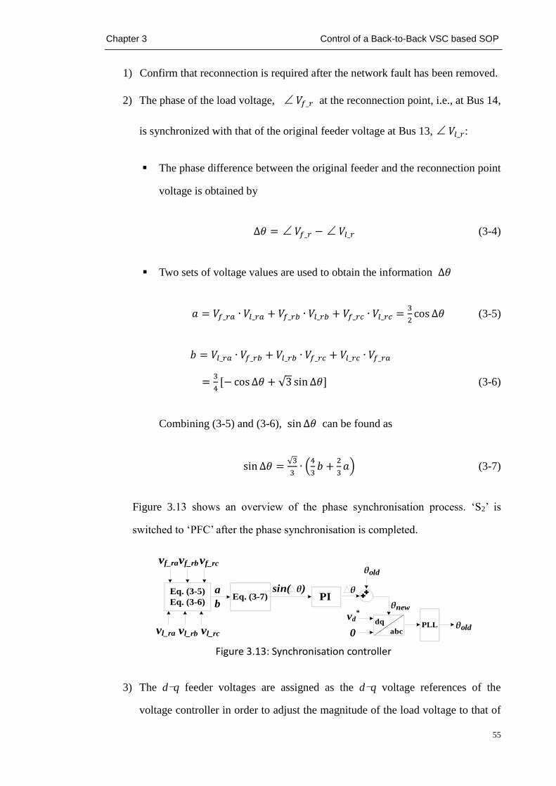
Chapter 3 Control of a Back-to-Back VSC based SOP
55
1) Confirm that reconnection is required after the network fault has been removed.
2) The phase of the load voltage, 𝑉𝑓_𝑟 at the reconnection point, i.e., at Bus 14,
is synchronized with that of the original feeder voltage at Bus 13, 𝑉𝑙_𝑟:
The phase difference between the original feeder and the reconnection point
voltage is obtained by
∆𝜃 = 𝑉𝑓_𝑟 − 𝑉𝑙_𝑟 (3-4)
Two sets of voltage values are used to obtain the information ∆𝜃
𝑎 = 𝑉𝑓_𝑟𝑎 ∙ 𝑉𝑙_𝑟𝑎 + 𝑉𝑓_𝑟𝑏 ∙ 𝑉𝑙_𝑟𝑏 + 𝑉𝑓_𝑟𝑐 ∙ 𝑉𝑙_𝑟𝑐 =3
2cos ∆𝜃 (3-5)
𝑏 = 𝑉𝑙_𝑟𝑎 ∙ 𝑉𝑓_𝑟𝑏 + 𝑉𝑙_𝑟𝑏 ∙ 𝑉𝑓_𝑟𝑐 + 𝑉𝑙_𝑟𝑐 ∙ 𝑉𝑓_𝑟𝑎
=3
4[− cos ∆𝜃 + √3 sin ∆𝜃] (3-6)
Combining (3-5) and (3-6), sin ∆𝜃 can be found as
sin ∆𝜃 =√3
3∙ (
4
3𝑏 +
2
3𝑎) (3-7)
Figure 3.13 shows an overview of the phase synchronisation process. ‘S2’ is
switched to ‘PFC’ after the phase synchronisation is completed.
Eq. (3-5)
Eq. (3-6)
vf_ra vf_rb vf_rc
a
bEq. (3-7)
sin( θ)PI
++
dq
abc
vd*
0 PLL
θ
vl_ra vl_rb vl_rc
θold
θnew
θold
Figure 3.13: Synchronisation controller
3) The d−q feeder voltages are assigned as the d−q voltage references of the
voltage controller in order to adjust the magnitude of the load voltage to that of

Chapter 3 Control of a Back-to-Back VSC based SOP
56
the grid voltage.
4) When both phase and magnitude of the output voltage match the original feeder
voltage, ‘S1’ is switched to ‘PFC’, and the isolated loads are reconnected to the
original feeder. To prevent large transient flows of real and reactive power, the
integers in both power and current controllers are reset and the reference values
of real and reactive power are set as the value before transfer to the power flow
control mode.
Figure 3.14 shows the synchronisation of the voltages when the synchronisation
algorithm started to work in the supply restoration mode. As can be seen, the
synchronisation process successfully forced the voltage at the end of the isolated area to
track the voltage at the original feeder.
(a)
(b)
Figure 3.14: Voltage synchronisations for reconnection: (a) phase synchronisation; (b)
magnitude synchronisation
-12.0
-8.0
-4.0
0.0
4.0
8.0
12.0
2.48 2.5 2.52 2.54 2.56 2.58 2.6
Vo
ltag
e (k
V)
Time (s)
Vf_ra
Vl_ra
0.0
4.0
8.0
12.0
2.6 2.62 2.64 2.66 2.68 2.7 2.72
Vo
ltag
e (k
V)
Time (s)
Vf_r
Vl_r

Chapter 3 Control of a Back-to-Back VSC based SOP
57
Figure 3.15 depicts the output voltage and current waveforms of the faulted side VSC
after using the synchronisation process. The current spike and voltage sag were
successfully reduced.
(a)
(b)
Figure 3.15: Results of a smooth transition to power flow control mode: (a) output
voltage waveform of the faulted side VSC; (b) output current waveform
3.5 Summary
Two control modes were developed for the operation of a back-to-back VSC based SOP.
For the power flow control mode, a dual closed-loop current-controlled strategy was
used to regulate both active and reactive power on the connected feeders. For the
supply restoration mode, a voltage and frequency control strategy was proposed to
-13.0
-10.0
-7.0
-4.0
-1.0
2.0
5.0
8.0
11.0
2.8 2.85 2.9 2.95 3 3.05 3.1 3.15 3.2
Vo
ltag
e (k
V)
Time (s)
-0.06
-0.04
-0.02
0.00
0.02
0.04
0.06
2.8 2.85 2.9 2.95 3 3.05 3.1 3.15 3.2
Cu
rren
t (k
A)
Time (s)

Chapter 3 Control of a Back-to-Back VSC based SOP
58
provide fast power supply restoration when the loads connected to one side of SOP are
isolated due to network faults. The operational principle of the back-to-back VSC based
SOP was analysed under both normal and abnormal network operating conditions. Case
studies based on a two-feeder MV distribution network evaluated the performance of
the SOP device with the two control modes under normal, faults and post-fault supply
restoration conditions.
Under normal conditions, the proposed SOP controller provides both instantaneous and
longer duration power flow regulation between the interconnected feeders and dynamic
Volt/VAR support on both terminals.
During fault conditions, the SOP controller (power flow control mode) is able to isolate
both balanced and unbalanced network faults between interconnected feeders. The SOP
is therefore capable of limiting both the fault propagation on the network and the
increase of the short-circuit current.
Under post-fault supply restoration conditions, the SOP device was demonstrated to be
effective in providing fast supply restoration through a smooth transition between the
power flow control and the supply restoration modes. For the transition from the power
flow control mode to the supply restoration mode, a soft cold load pickup process was
preferred over the hard transition. The soft cold load pickup process removed the DC
offset and inrush problems of the output current which may trigger unexpected
protection operations. For the transition from the supply restoration mode to the power
flow control mode, the undesirable current impulse and voltage drop were reduced after
the use of the voltage synchronisation procedure and the reset of current and power
controllers.

Chapter 4 Benefits Analysis of SOPs for MV Distribution Network Operation
59
Benefits Analysis of SOPs for
MV Distribution Network
Operation
HIS chapter investigates the operational benefits of SOPs for MV
distribution network operation including power loss minimization,
feeder load balancing and voltage profile improvement.
Chapter 4
T

Chapter 4 Benefits Analysis of SOPs for MV Distribution Network Operation
60
4.1 Introduction
In this chapter, a steady state analysis framework was developed to quantify the
operational benefits of a MV distribution network with SOPs.
A generic power injection model of an SOP for steady state analysis was developed,
which takes into account both physical limitations and internal power losses of the SOP
device, using back-to-back VSCs. Based on the SOP model, an improved Powell’s
direct set method was developed to obtain the optimal SOP operation. Distribution
network reconfiguration algorithms, with and without SOPs, were also developed and
used to identify the benefits of using SOPs.
The performance of using SOPs, traditional network reconfiguration and the
combination of both was compared and analysed based on a 33-bus distribution
network. The impact of DG connections and the impact of SOP device losses were also
evaluated through quantitative and sensitive analysis.
4.2 Modelling of Soft Open Points
Figure 4.1a shows a typical location of an SOP which allows power electronic devices
to control active power flow between connected feeders and to supply or absorb
reactive power at its interface terminals under normal network operating conditions. A
generic power injection model of SOP was developed. This model considers SOP
terminal power injections and hence enables the incorporation of SOPs into existing
power flow analysis algorithms without considering the detailed controller design.

Chapter 4 Benefits Analysis of SOPs for MV Distribution Network Operation
61
(a)
(b)
Figure 4.1: (a) Simple distribution network with an SOP; (b) Power injection model of
SOP for distribution network power flow control
Figure 4.1b shows the representation of an SOP model with real and reactive power,
injecting into feeders I and J through both terminals. Taking these power injections as
decision variables, the power flow in feeder I is calculated by the following set of
recursive equations [93]:
𝑃𝑖 = 𝑃𝑖−1 − 𝑃𝐿𝑜𝑠𝑠 (𝑖−1, 𝑖) − 𝑃𝐿,𝑖 = 𝑃𝑖−1 −𝑟𝑖−1
|𝑉𝑖−1|2∙ (𝑃𝑖−1
2 + 𝑄𝑖−12) − 𝑃𝐿,i (4-1)
𝑄𝑖 = 𝑄𝑖−1 − 𝑄𝐿𝑜𝑠𝑠 (𝑖−1, 𝑖) − 𝑄𝐿,𝑖 = 𝑄𝑖−1 −𝑥𝑖−1
|𝑉𝑖−1|2∙ (𝑃𝑖−1
2 + 𝑄𝑖−12) − 𝑄𝐿,i (4-2)
|𝑉𝑖|2 = |𝑉𝑖−1|2 − 2 ∙ (𝑟𝑖−1𝑃𝑖−1 + 𝑥𝑖𝑄𝑖) +
(𝑟𝑖−12+𝑥𝑖−1
2)
|𝑉𝑖−1|2∙ (𝑃𝑖−1
2 + 𝑄𝑖−12) (4-3)

Chapter 4 Benefits Analysis of SOPs for MV Distribution Network Operation
62
with boundary conditions:
|𝑃𝑛 + 𝑃𝑆_𝑖𝑛𝑗𝐼 | = 𝑃𝐿𝑜𝑠𝑠 (𝑛, 𝑠𝐼) (4-4)
|𝑄𝑛 + 𝑄𝑆_𝑖𝑛𝑗𝐼 | = 𝑄𝐿𝑜𝑠𝑠 (𝑛, 𝑠𝐼) (4-5)
where 𝑃 represents active power, 𝑄 reactive power, 𝑉 nodal voltage, 𝑟 resistance
and 𝑥 reactance. Subscript 𝐿𝑜𝑠𝑠 denotes line losses, and 𝐿 denotes load. The
variables and parameters are shown in Figure 4.1b. Similar recursive power flow
equations with boundary conditions are applied to feeder J.
To consider the internal losses of the SOP equipment, the following equality constraint
of power balance is used:
𝑃𝑆_𝑖𝑛𝑗𝐼 + 𝑃𝑆_𝑖𝑛𝑗
𝐽 + 𝑃𝑆𝑂𝑃,𝐿𝑜𝑠𝑠 = 0 (4-6)
where 𝑃𝑆𝑂𝑃,𝐿𝑜𝑠𝑠 denotes the internal power losses of the whole SOP device.
Various types of power electronic devices can be implemented as an SOP, such as
UPFC, back-to-back VSCs and multi-terminal VSCs. In this work, back-to-back VSCs
were used. Constraints of such device due to the physical limitations and the internal
power losses are formulated as follows.
4.2.1 Physical Limitations of Back-to-Back Converters
As described in Section 2.3, back-to-back VSCs consist of two VSCs connected via a
DC link. Both VSCs are able to provide fast and independent control of active and
reactive power in all four quadrants of the P-Q plane. The terminal power injections of
back-to-back VSCs operated as a SOP are controlled directly by each VSC, the
operational limits of VSC capacity and terminal voltage are considered as:

Chapter 4 Benefits Analysis of SOPs for MV Distribution Network Operation
63
√ 𝑃𝑆_𝑖𝑛𝑗𝐼 2
+ 𝑄𝑆_𝑖𝑛𝑗𝐼 2
≤ 𝑆𝑉𝑆𝐶,𝑟𝑎𝑡𝑒𝐼 (4-7)
𝑉𝑠𝐼 ≤ 𝑉𝑉𝑆𝐶,𝑟𝑎𝑡𝑒𝐼 (4-8)
where 𝑆𝑉𝑆𝐶,𝑟𝑎𝑡𝑒𝐼 is the power rating of the VSC connected to feeder I; 𝑉𝑠𝐼
and 𝑉𝑉𝑆𝐶,𝑟𝑎𝑡𝑒𝐼 denote the actual and maximum AC terminal voltage. Similar constraints
are applied to the other side VSC connected to feeder J.
4.2.2 Internal Power Losses of Back-to-Back Converter
Internal power losses of the back-to-back device are made up of the losses of its
individual components, including the semiconductors (conduction and switching
losses), passive components (DC link capacitor, filter, AC line choke), transformers and
the cooling system.
As suggested in [94], these losses can be categorized into three components: no load
losses, linear and quadratic losses depending on the converter current, which is a
function of the active and reactive power exchanged with the AC network:
𝑃𝑉𝑆𝐶,𝐿𝑜𝑠𝑠𝐼 = 𝑎𝐼 ∙ 𝐼𝑉𝑆𝐶
𝐼 2+ 𝑏𝐼 ∙ 𝐼𝑉𝑆𝐶
𝐼 + 𝑐𝐼 (4-9)
𝐼𝑉𝑆𝐶𝐼 =
√ 𝑃𝑆_𝑖𝑛𝑗𝐼 2
+ 𝑄𝑆_𝑖𝑛𝑗𝐼 2
|𝑉𝑠𝐼| (4-10)
where 𝑃𝑉𝑆𝐶,𝐿𝑜𝑠𝑠𝐼 and 𝐼𝑉𝑆𝐶
𝐼 represent the power losses and the AC current of the VSC
connecting to feeder I. Similar equations are applied to the other side VSC. Thus all
equations shown in the following section only illustrate the VSC connected to feeder I.
As shown in (4-9), the total losses are determined by the coefficients, 𝑎𝐼, 𝑏𝐼and 𝑐𝐼.
These coefficients are difficult to obtain due to the limited information from the open
literature or manufacturers. Usually only the internal power losses (or efficiency) under

Chapter 4 Benefits Analysis of SOPs for MV Distribution Network Operation
64
nominal conditions (rated power) and the no load loss, 𝑐𝐼are given.
A linear function is used to approximate the quadratic one in (4-9):
𝑃𝑉𝑆𝐶,𝐿𝑜𝑠𝑠𝐼 = 𝑘𝐼 ∙ 𝐼𝑉𝑆𝐶
𝐼 + 𝑐𝐼 (4-11)
𝑘𝐼 = (𝑃𝑉𝑆𝐶,𝐿𝑜𝑠𝑠,𝑟𝑎𝑡𝑒𝐼 − 𝑐𝐼)/𝐼𝑉𝑆𝐶,𝑟𝑎𝑡𝑒
𝐼 (4-12)
where 𝑃𝑉𝑆𝐶,𝐿𝑜𝑠𝑠,𝑟𝑎𝑡𝑒𝐼 and 𝐼𝑉𝑆𝐶,𝑟𝑎𝑡𝑒
𝐼 are power losses and AC current of the VSC
connected to feeder I under nominal condition.
Comparing the internal power losses derived from (4-9) and (4-11), as shown in Figure
4.2, it is noted that when 𝐼𝑉𝑆𝐶𝐼 ≤ 𝐼𝑉𝑆𝐶,𝑟𝑎𝑡𝑒
𝐼 , the device power losses using the
approximate model are higher than those using the quadratic one, i.e., more
conservative conclusions are drawn. Therefore, the approximate model was used in this
work.
Figure 4.2: Comparison between the quadratic and approximate loss estimation
function

Chapter 4 Benefits Analysis of SOPs for MV Distribution Network Operation
65
4.3 Optimal Operation of the Soft Open Points
The benefits of SOPs for both system loss reduction and feeder load balancing were
investigated. To quantify these benefits, the amounts of real and reactive power
injections of the SOPs were determined through solving a combinational nonlinear
constrained optimization problem.
4.3.1 Problem Formulation
Two objective functions are used separately to quantify the optimality of the SOP
operation.
Active power loss minimization
The active power losses consist of two components: the feeder losses and the internal
power losses of the SOP devices. The active power loss minimization problem is
formulated as:
Minimize 𝑃𝑇,𝐿𝑜𝑠𝑠 = ∑ 𝑟𝑘 ∙𝑃𝑘
2+𝑄𝑘2
|𝑉𝑘|2
𝑛𝑙𝑘=1 + 𝑃𝑆𝑂𝑃,𝐿𝑜𝑠𝑠 (4-13)
where 𝑟𝑘 , 𝑃𝑘 , 𝑄𝑘 , 𝑉𝑘 are resistance, active power, reactive power, and voltage of
branch k; and 𝑛𝑙 is the total number of branches in the network.
Feeder load balancing
A branch loading index 𝐿𝐼𝑘 is used to measure the loading level of each branch in the
network, which is expressed as:
𝐿𝐼𝑘 = (𝐼𝑘
𝐼𝑘,𝑟𝑎𝑡𝑒)
2
∀ 𝑘 ∈ 𝑛𝑙 (4-14)
where 𝐼𝑘 and 𝐼𝑘,𝑟𝑎𝑡𝑒 are the actual and the rated branch current of branch k.
Feeder load balancing is achieved by minimizing the load balance index 𝐿𝐵𝐼, which is
defined as the sum of branch load balancing indices, as shown in (4-15):

Chapter 4 Benefits Analysis of SOPs for MV Distribution Network Operation
66
𝑀𝑖𝑛𝑖𝑚𝑖𝑧𝑒 𝐿𝐵𝐼 = ∑ 𝐿𝐼𝑘𝑛𝑙𝑘=1 (4-15)
Constraints
Constraints of the distribution network and the SOP devices are considered. The device
constraints of each SOP are shown in (4-6)-(4-8). The network constraints are
expressed as follows:
𝑔(𝑥, 𝑠) = 0 (4-16)
|𝑉𝑖,𝑚𝑖𝑛| ≤ |𝑉𝑖| ≤ |𝑉𝑖,𝑚𝑎𝑥| ∀ 𝑖 ∈ 𝑛𝑏 (4-17)
|𝑆𝑘| ≤ |𝑆𝑘,𝑚𝑎𝑥| ∀ 𝑘 ∈ 𝑛𝑙 (4-18)
where 𝑔(𝑥, 𝑠), 𝑉𝑖,𝑚𝑖𝑛, 𝑉𝑖,𝑚𝑎𝑥 and 𝑆𝑘,𝑚𝑎𝑥 are the power flow equations, the minimum
and the maximum voltage of bus i and the maximum capacity allowed in branch k. 𝑛𝑏
are the total number of buses of the network.
Penalty function
Constrains of mentioned above are included into the objective function by using the
penalty function method. In this way, unconstrained optimization methods are used
directly by solving the transformed objective function (with penalty terms):
𝑀𝑖𝑛𝑖𝑚𝑖𝑧𝑒 𝐹𝑜𝑏𝑗(𝑺) = {𝑃𝑇,𝐿𝑜𝑠𝑠 𝑜𝑟 𝐿𝐵𝐼} + 𝑘1 ∙ 𝑓𝑆𝑂𝑃 + 𝑘2 ∙ 𝑓𝑉 + 𝑘3 ∙ 𝑓𝑆 (4-19)
where 𝑘1, 𝑘2, 𝑘3 are the penalty constants; 𝑓𝑆𝑂𝑃 , 𝑓𝑉 , and 𝑓𝑆 are the penalty functions
for violations of the SOP device constraints, the network voltage and capacity
constraints; S denotes the decision variable vector.
Based on the power injection model of SOP in Section 4.2, the real and reactive power
injections at both terminals are specified as the decision variables: with one SOP
installation, 𝑺 = [𝑃𝑆𝑖𝑛𝑗
𝐼 , 𝑄𝑆𝑖𝑛𝑗
𝐼, 𝑄𝑆𝑖𝑛𝑗
𝐽 ]T. 𝑃𝑆_𝑖𝑛𝑗𝐽 is not included in 𝑺 since it is determined if

Chapter 4 Benefits Analysis of SOPs for MV Distribution Network Operation
67
𝑺 is specified according to the equality constraint equation of (4-6). Therefore, the
coordinates of n SOPs are combined together sequentially to obtain a point of 𝑺 in a
3n-dimentional space, thus
𝑺 = [𝑃𝑆_𝑖𝑛𝑗, 1𝐼 , 𝑄𝑆_𝑖𝑛𝑗, 1
𝐼, 𝑄𝑆_𝑖𝑛𝑗, 1
𝐽, 𝑃𝑆_𝑖𝑛𝑗, 2
𝐼 , 𝑄𝑆_𝑖𝑛𝑗, 2𝐼
, 𝑄𝑆_𝑖𝑛𝑗, 2𝐽
,
… , 𝑃𝑆𝑖𝑛𝑗, 𝑛𝐼 , 𝑄𝑆𝑖𝑛𝑗, 𝑛
𝐼 , 𝑄𝑆𝑖𝑛𝑗, 𝑛𝐽 ]T (4-20)
4.3.2 Method of Determining Optimal SOP Operation
Based on the Powell’s Direct Set (PDS) method presented in [95], an improved PDS
method to optimize the SOP operation was developed. The performance improvement
is achieved by obtaining a good initial approximated SOP operation.
Powell’s Direct Set method
Most mathematical optimization methods require expressions of the derivatives to
define the direction of movement, i.e. search the direction approaching to the optimum
(from a starting point).
The Powell’s Direct Set method is a direct search method proposed by Powell et al.
[95]. It defines the search directions in a direct manner, i.e., solely depending on the
objective function itself. Therefore, this method is easy to implement and is not limited
by the existence of derivatives of the objective function. It has been successfully
applied to solve problems for which it is difficult or impossible to calculate the
derivatives [96-98].
A comprehensive review of PDS method as well as the mathematical proof of its
convergence were given in [95]. Three key properties of this method are highlighted
below:

Chapter 4 Benefits Analysis of SOPs for MV Distribution Network Operation
68
i. For an N-dimensional problem, minimization is achieved by an iterative procedure
that searches down N linear independent directions within each iteration, i.e.
starting from the best known approximation to the optimum.
ii. Fast convergence to the optimum is achievable by only searching down N mutually
conjugate directions. The optimal solution of a quadratic function has been proved
achievable by searching along those mutually conjugate directions once only.
Hence only N iterations are required to solve the N-dimensional quadratic problem
[95]. The efficacy has also been demonstrated for any other function forms, as
presented in [96, 97], but may require more iterations.
iii. The mutually conjugate directions are generated after each iteration, as illustrated
in the following part.
PDS method for optimal SOP operation
The process of determining optimal SOP operation using the PDS method is shown in
Figure 4. 3.
(1) Initialization
(2) Generate a new mutually conjugate direction ƺConju.
(4) Find the minimum of Fobj along the conjugate direction ƺConju.
(5)Stopping rule satisfied?
(6) Output the results:
Fobj and SOP operation S;
(7) End
No
Yes
(3) Update the search direction set {ƺ} ?
Yes
No
Figure 4.3: Flow chart of the proposed PDS method

Chapter 4 Benefits Analysis of SOPs for MV Distribution Network Operation
69
STEP 1): Initialization. Based on (4-20), the initial approximate SOP operation 𝑺𝟎(1)
,
the initial search direction set with 3n linear independent search directions, {𝝃}(𝟏) =
{ 𝝃𝟏(1)
, … , 𝝃𝒊(1)
, … , 𝝃𝟑𝒏(1)
} and the convergence criterion 𝜀 are specified. The 3n
directions in {𝝃}(𝟏) are initially chosen to be the co-ordinate directions (linear
independent). This means only one decision variable in (4-20) will be changed when
searching along one direction.
STEP 2): Generate a new mutually conjugate direction within one iteration. There are
two sub steps:
i. Starting from 𝑺𝟎(𝑘)
, k indicates the iteration number (one iteration includes
searching along 3n directions, k=1 initially), sequentially find 𝑺𝒊(𝒌)
which gives
the minimum of the objective function (4-19) along each search direction, 𝝃𝒊(𝑘)
in {𝝃}(𝒌), which is expressed as:
Min 𝐹𝑜𝑏𝑗(𝑺𝒊(𝑘)
) = 𝐹𝑜𝑏𝑗(𝑺𝒊−𝟏(𝑘)
+ 𝜆𝑖 ∙ 𝝃𝒊(𝑘)
), i=1, 2,…, 3n (4-21)
In this work, a one-dimensional search method, the golden section search [95],
was adopted to calculate the optimal step size, 𝜆𝑖. The load flow analysis method
introduced in [99] combined with the SOP injection model formulated in (4-1) -
(4-6) was implemented as a subroutine to calculate the objective function
𝐹𝑜𝑏𝑗(𝑺𝒊(𝑘)
) in (4-21).
ii. After searching down the 3n directions, a conjugate direction is generated by
(4-22)
𝝃𝒄𝒐𝒏𝒋𝒖.(𝑘)
= 𝑺𝟑𝒏(𝑘)
− 𝑺𝟎(𝑘)
(4-22)

Chapter 4 Benefits Analysis of SOPs for MV Distribution Network Operation
70
STEP 3): Update the search direction set for the next iteration {𝝃}(𝒌+𝟏). Two scenarios
are considered:
i. If n=1, discard the first direction 𝝃𝟏(𝑘)
in { 𝝃𝒊(𝑘)
} by adding 𝝃𝒄𝒐𝒏𝒋𝒖.(𝑘)
to the end,
as shown in (4-23):
{𝝃}(𝒌+𝟏) = { 𝝃𝟐(𝑘)
, 𝝃𝟑(𝑘)
, … , 𝝃𝟑𝒏(𝑘)
, 𝝃𝒄𝒐𝒏𝒋𝒖.(𝑘)
} (4-23)
ii. If n>1, a ‘smarter’ updating procedure is required to ensure a reasonable rate of
convergence, i.e., replace the direction in {𝝃}(𝒌) , which shows the worst
performance. The general procedure is presented as follows [95]:
Find 𝝃𝒎(𝑘)
that gives maximum reduction among the previous
one-dimensional searching processes in Step 2, as shown in (4-24):
∆𝑚𝑎𝑥= 𝑀𝑎𝑥𝟏≤𝒎≤𝟑𝒏
{ 𝐹𝑜𝑏𝑗(𝑺𝒎−𝟏(𝑘)
) − 𝐹𝑜𝑏𝑗(𝑺𝒎(𝑘)
)} (4-24)
Replace 𝝃𝒎(𝑘)
by 𝝃𝒄𝒐𝒏𝒋𝒖.(𝑘)
to give more efficient convergence if the
following two criterions are satisfied:
(𝑤1 − 2𝑤2 + 𝑤3)(𝑤1 − 𝑤2 − ∆𝑚𝑎𝑥)2 < 0.5 ∙ ∆𝑚𝑎𝑥(𝑤1 − 𝑤3)2
𝑤3 < 𝑤1} (4-25)
where 𝑤1 = 𝐹𝑜𝑏𝑗(𝑺𝟎(𝑘)
), 𝑤2 = 𝐹𝑜𝑏𝑗 (𝑺𝟑𝒏(𝑘)
),𝑤3 = 𝐹𝑜𝑏𝑗 (2 ∙ 𝑺𝟑𝒏(𝑘)
− 𝑺𝟎(𝑘)
). Thus,
{𝝃}(𝒌+𝟏) = { 𝝃𝟏(𝑘)
, … , 𝝃𝒎−𝟏(𝑘)
, 𝝃𝒄𝒐𝒏𝒋𝒖.(𝑘)
, 𝝃𝒎+𝟏(𝑘)
, … , 𝝃𝟑𝒏(𝑘)
} (4-26)
Otherwise{𝝃}(𝒌)is not updated in this iteration, let 𝑺𝟎(𝑘+1)
= 𝑺𝟑𝒏(𝑘)
and jump
to Step 5.

Chapter 4 Benefits Analysis of SOPs for MV Distribution Network Operation
71
STEP 4): Search down along the conjugate direction. Calculate 𝜆 as (4-21) so
that 𝐹𝑜𝑏𝑗( 𝑺𝟎(𝑘+1)
) reaches its minimum along the conjugate direction generated in
(4-22). Let 𝑺𝟎(𝑘+1)
= 𝑺𝟑𝒏(𝑘)
+ 𝜆 ∙ 𝝃𝒄𝒐𝒏𝒋𝒖.(𝑘)
.
STEP 5): Convergence check. If ‖ 𝑺𝟎(𝑘+1)
− 𝑺𝟎(𝑘)
‖ > 𝜀, let k=k+1 and then go to Step 2,
else stop.
An example shown in Figure 4.4 illustrates the searching of the optimization process.
As the red solid line shows, the optimization starts from an initial approximation 𝑺𝟎(1)
and then reaches the minimum 𝑺𝟏(1)
, 𝑺𝟐(1)
, 𝑺𝟑(1)
along each of the coordinate directions
in {𝝃}(𝟏). The first conjugate direction 𝝃𝒄𝒐𝒏𝒋𝒖.(1)
is hence obtained, as shown by the blue
dotted arrow. After searching along the conjugate direction, a new approximation 𝑺𝟎(2)
is obtained for the second iteration.
Figure 4.4: Example of one SOP optimization by PDS method

Chapter 4 Benefits Analysis of SOPs for MV Distribution Network Operation
72
Determine the initial approximated SOP operation
The PDS method is able to start from any initial point 𝑺𝟎(1)
. A good approximation of
SOP operation is obtained by running the PDS method once using the objective
function of (4-21) with simplified power flow equations given by [99]:
i. All nodal voltage magnitudes are assumed to be 1 p.u., equations (4-13) and
(4-15) are reduced to
𝑃𝐿𝑜𝑠𝑠 ≈ ∑ 𝑟𝑘 ∙ (𝑃𝑘2 + 𝑄𝑘
2) + 𝑃𝑆𝑂𝑃,𝐿𝑜𝑠𝑠𝑛𝑙𝑘=1 (4-27)
𝐿𝐼𝐵 ≈ ∑𝑃𝑘
2+𝑄𝑘2
𝐼𝑘,𝑟𝑎𝑡𝑒2
𝑛𝑙𝑘=1 (4-28)
ii. Ignoring all the quadratic terms (line losses) from the power flow
equations in (4-1)-(4-3). The branch power 𝑃𝑘 and 𝑄𝑘 are obtained by
summing up the downstream power loads:
𝑃𝑘 ≈ ∑ 𝑃𝐿,𝑖𝑛𝑖=𝑘+1 (4-29)
𝑄𝑘 ≈ ∑ 𝑄𝐿,𝑖𝑛𝑖=𝑘+1 (4-30)
The constraints of nodal voltage and branch capacity are considered by:
|𝑉𝑖|2 ≈ |𝑉0|2 − 2 ∑ (𝑟𝑘𝑃𝑘 + 𝑥𝑘𝑄𝑘) ≤ 𝑉𝑚𝑎𝑥
2𝑖𝑘=1 (4-31)
𝑆𝑘 ≈ (𝑃𝑘2 + 𝑄𝑘
2) ≤ 𝑆𝑘,𝑚𝑎𝑥2 (4-32)
Using the simplified equations, as shown in (4-27)-(4-32), the initial approximated SOP
operation is able to be obtained directly without using the accurate load flow
calculations.

Chapter 4 Benefits Analysis of SOPs for MV Distribution Network Operation
73
4.4 Network Reconfiguration Considering SOPs
Reconfiguring distribution networks is used to achieve better network operation
including power loss minimization, feeder load balancing and supply restoration. To
investigate the performance of distribution network reconfiguration when SOPs are
installed to replace some of the normally-open points, the proposed PDS method for
optimal SOP operation was combined with the network reconfiguration method
introduced in [34].
The procedure of the combined algorithm is given in Figure 4.5.
Start
Determine the sequence of load busbars to search supply paths
Find the optimal network configuration using a shortest path search algorithm
Calculate the combined results as fitness values
Stopping criteria is satisfied?
Output optimization results
End
GA algorithm
with
Selection,
crossover and
mutation
Yes
No
Determine optimal SNOP operation using the PDS method
Figure 4.5: Flowchart of proposed network reconfiguration considering SOPs

Chapter 4 Benefits Analysis of SOPs for MV Distribution Network Operation
74
According to [34], a shortest-path algorithm is used to find the optimal electricity
supply path for each load busbar. A genetic algorithm (GA) with the selection,
crossover and mutation operators is used to optimize the sequence of load busbars
searching for the supply paths because the sequence affects the obtained network
configurations. The improved PDS method for optimal SOP operation is integrated
after the shortest path algorithm. The fitness functions are formulated in Section 4.3.1.
4.5 Case Study
A 33-bus distribution network, as shown in Figure 4.6, was used for case study [99].
This network has 32 normally-closed switches, 5 normally-open switches and the
nominal voltage is 12.66 kV. The total real and reactive power loads are 3,715 kW and
2,300 kVar. Four normally-open switches, i.e., the switches between buses 25 and 29,
33 and 18, 8 and 21, 12 and 22, were chosen as candidate places for SOP installation.
The size of each SOP unit was assumed to be 3 MVA. Such a large size is chosen to
ensure enough capacity for SOP operations under all studied network conditions.
Figure 4.6: 33-bus distribution network [99]
Four cases were defined and used for quantifying the benefits of SOPs for improvement
of network performance:

Chapter 4 Benefits Analysis of SOPs for MV Distribution Network Operation
75
Case I: Improve network performance using SOPs;
Case II: Improve network performance considering both SOPs and network
reconfiguration;
Case III: Impacts of DG connections;
Case IV: Impact of power losses of SOP devices.
4.5.1 Improve Network Performances Using SOPs
The impact of different number of SOPs installed in the network on both power loss
minimization and feeder load balancing was investigated. The device power losses
were ignored for this case.
Power loss minimization
Figure 4.7a shows the results of minimized power losses with 1 to 4 SOPs installed in
the network. There was a significant reduction (by 42%) of the system power loss with
one SOP installation. With more SOPs installed in the system, the total power losses
were further reduced (by 57%).The voltage profiles of the system were also improved
with the SOP installations, as shown in Figure 4.7b.
(a)
0
60
120
180
240
0 1 2 3 4
Tota
l Po
wer
Lo
sses
(kW
)
Number of SOP
Effect of Number of SOP Installation on Power Loss
No. SOP Locations (Branches)1 25-292 25-29 18-333 25-29 18-33 12-22 4 25-29 18-33 12-22 8-21

Chapter 4 Benefits Analysis of SOPs for MV Distribution Network Operation
76
(b)
Figure 4.7: Impact of different number of SOP installation on power loss minimization
and voltage profile improvement
Feeder load balancing
One feeder of the network from branch L25 to branch L32 as shown in Figure 4.8 was
assumed to be heavily loaded, i.e., 1.6 times higher than the loading under the normal
condition. Table 4.1 shows the impact of different number of SOPs on feeder load
balancing. It is observed that the system load balancing index LBI was reduced by
47.73% with one SOP. Although the LBI reduction was further improved with more
SOPs installed, the rate of improvement was diminishing.
Table 4.1: System Load Balancing Index with Different Number of SOP Installation
Number of SOP Installed 0 1 2 3 4
SOP Locations (Branches)
_ 25-29 25-29
18-33
25-29
18-33
12-22
26-29
18-33
12-22
8-21
System Load Balancing Index 6.156 3.218 2.566 2.428 2.389
% LBI Reduction − 47.726 58.317 60.056 61.192
0.88
0.9
0.92
0.94
0.96
0.98
1
1 4 7 10 13 16 19 22 25 28 31
Vo
ltag
e (p
.u.)
Bus Number
Impact of Number of SOP Installation on System Voltage Profile
0 SOP 1 SOP 2 SOP 3 SOP 4 SOP

Chapter 4 Benefits Analysis of SOPs for MV Distribution Network Operation
77
Figure 4.8a illustrates the branch loading profile of the network. By using SOPs, the
loading of those heavily loaded branches (e.g. branches L1 to L6 and L25 to L30) was
reduced dramatically by transferring loads to the lightly loaded branches via SOP
control. As a consequence, the loading levels from branches L12 to L24 were increased.
The voltage profile was also improved, as shown in Figure 4.8b. The minimum bus
voltage (at bus 32) was 0.88 p.u. due to overloading, and it was improved by 9.09%
after the system loading was balanced using SOPs.
(a)
(b)
Figure 4.8: Impact of different number of SOP installation on load balancing and
voltage profile improvement
0
0.2
0.4
0.6
0.8
1
1.2
1 3 5 7 9 11 13 15 17 19 21 23 25 27 29 31
Bra
nch
Lo
adin
g
Branch Number
Impact of Number of SOP Installation on Load Balancing
0 SOP 1 SOP 2 SOP 3 SOP 4 SOP
0.86
0.88
0.90
0.92
0.94
0.96
0.98
1.00
1 3 5 7 9 11 13 15 17 19 21 23 25 27 29 31 33
Vo
ltag
e (p
.u.)
Bus Number
Impact of Number of SOP Installation on System Voltage Profile
0 SOP 1 SOP 2 SOP 3 SOP 4 SOP
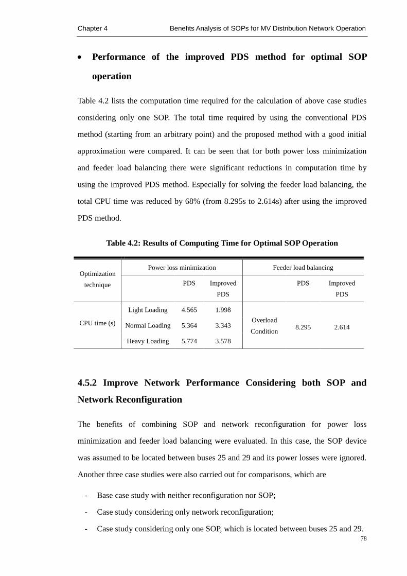
Chapter 4 Benefits Analysis of SOPs for MV Distribution Network Operation
78
Performance of the improved PDS method for optimal SOP
operation
Table 4.2 lists the computation time required for the calculation of above case studies
considering only one SOP. The total time required by using the conventional PDS
method (starting from an arbitrary point) and the proposed method with a good initial
approximation were compared. It can be seen that for both power loss minimization
and feeder load balancing there were significant reductions in computation time by
using the improved PDS method. Especially for solving the feeder load balancing, the
total CPU time was reduced by 68% (from 8.295s to 2.614s) after using the improved
PDS method.
Table 4.2: Results of Computing Time for Optimal SOP Operation
Optimization
technique
Power loss minimization Feeder load balancing
PDS Improved
PDS
PDS Improved
PDS
CPU time (s)
Light Loading 4.565 1.998
Overload
Condition
8.295
2.614 Normal Loading 5.364 3.343
Heavy Loading 5.774 3.578
4.5.2 Improve Network Performance Considering both SOP and
Network Reconfiguration
The benefits of combining SOP and network reconfiguration for power loss
minimization and feeder load balancing were evaluated. In this case, the SOP device
was assumed to be located between buses 25 and 29 and its power losses were ignored.
Another three case studies were also carried out for comparisons, which are
- Base case study with neither reconfiguration nor SOP;
- Case study considering only network reconfiguration;
- Case study considering only one SOP, which is located between buses 25 and 29.

Chapter 4 Benefits Analysis of SOPs for MV Distribution Network Operation
79
Power loss minimization
The network performance on power loss minimization was simulated under three
loading conditions: light (50%), normal (100%), and heavy (160%). The simulation
results are listed in Table 4.3.
Table 4.3: Results of Different Methods for System Power Loss
Case Studies
Load Level
Light (0.5) Normal (1.0) Heavy
(1.6)
Base Case
No reconfiguration
No SOP installed
Switches with open status 8-21 12-22 25-29 9-15 18-33
Power Loss (kW) 47.118 202.876 575.966
Minimum Voltage (p.u.) 0.958 0.913 0.853
Only network
reconfiguration
Switches Opened 7-8 9-10 14-15 25-29 32-33
Power Loss (kW) 33.312 137.946 381.418
% Loss reduction 29.301 32.005 33.778
Minimum Voltage (p.u.) 0.970 0.938 0.897
Only SOP
Switches with open status 8-21 12-22 9-15 18-33
SOP
Operation
𝑃𝑆_𝑖𝑛𝑗1 / MW 0.230 0.605 0.998
𝑄𝑆_𝑖𝑛𝑗1 / MVar 0.225 0.471 0.784
𝑄𝑆_𝑖𝑛𝑗2 / MVar 0.610 1.239 2.017
Power Loss (kW) 29.774 124.456 337.525
% Loss reduction 36.810 38.653 41.398
Minimum Voltage (p.u.) 0.967 0.933 0.890
Combined
network
reconfiguration
with SOP
Switches with open status 7-8 9-10 14-15 18-33
SOP
Operation
𝑃𝑆_𝑖𝑛𝑗1 / MW 0.183 0.374 0.607
𝑄𝑆_𝑖𝑛𝑗1 / MVar 0.215 0.424 0.697
𝑄𝑆_𝑖𝑛𝑗2 / MVar 0.516 1.045 1.686
Power Loss (kW) 22.758 93.915 250.179
% Loss reduction 51.700 53.708 56.564
Minimum Voltage (p.u.) 0.978 0.955 0.925

Chapter 4 Benefits Analysis of SOPs for MV Distribution Network Operation
80
The percentages of total power loss reduction implies that using only one SOP
achieved a similar power loss reduction to that of network reconfiguration under three
loading conditions. The most significant power loss reductions and voltage
improvement under all three loading conditions were obtained using the combined
method. The SOP operation required to achieve power loss minimization indicates that
the combined method contributed more to power loss reduction while requiring smaller
SOP sizes.
Figure 4.9 illustrates the voltage profiles of all case studies under the normal loading
condition. The shapes of the voltage profile under the other two loading condition were
the same except minor change in magnitude, and hence are not illustrated.
Figure 4.9: Voltage profiles of the network under normal loading condition
Feeder load balancing
The same overloading condition described in the previous case study was simulated.
Table 4.4 presents the load balancing index for the four case studies. The branch
loading profiles and voltage profiles are shown in Figure 4.10. From these results, it is
seen that by using only one SOP to control network power flows achieved better
performance on load balancing than that of using network reconfiguration to change the
0.88
0.9
0.92
0.94
0.96
0.98
1
1 3 5 7 9 11 13 15 17 19 21 23 25 27 29 31 33
Vo
ltag
e (p
.u.)
Bus Number
Volatage Profile of 33-bus Distribution Netwo at Normal Load
Base Case Only Reconfiguration
Only SOP Combined Method

Chapter 4 Benefits Analysis of SOPs for MV Distribution Network Operation
81
open/close status of a sequence of switches. The highest LBI reduction, i.e., the most
well-balanced network, and the highest improvement on minimum voltage were
achieved using the combined method.
Table 4.4: Results of Different Methods for Load Balancing
Case Studies Base
Case
Only network
reconfiguration
Only
SOP
Combined
reconfiguration with SOP
System load balancing index 6.156 4.139 3.218 2.594
LBI reduction (%) - 32.765 47.726 68.337
Minimum Voltage (p.u.) 0.880 0.904 0.928 0.943
SOP
Operation
𝑷𝑺_𝒊𝒏𝒋𝟏 / MW - - 0.916 1.142
𝑸𝑺_𝒊𝒏𝒋𝟏 / MVar - - 0.569 0.577
𝑸𝑺_𝒊𝒏𝒋𝟐 / MVar - - 1.791 2.417
(a)
0
0.3
0.6
0.9
1.2
1 3 5 7 9 11 13 15 17 19 21 23 25 27 29 31
Bra
nch
Lo
adin
g
Branch Number
Branch Loading Using Different Methods for Load Balancing
Base Case Only Reconfiguration
Only SOP Combined Method

Chapter 4 Benefits Analysis of SOPs for MV Distribution Network Operation
82
(b)
Figure 4.10: Results of load balancing capability and relevant voltage profile
improvement under different methods
4.5.3 Impact of DG Connections
A large capacity of intermittent renewable energy in the distribution network can
aggravate feeder loads unbalance and network power losses. To evaluate the benefits of
using the SOP for power loss minimization and feeder load balancing with DG
connections, three DGs were assumed to be connected to buses 16, 17 and 18. Each DG
had a power production of 1 MW with a unity power factor and was modelled as a
negative load in this study. An SOP was assumed to be located between buses 18 and
33 and its power losses were ignored. Five case studies were carried out for
comparisons, which are
− Base case study with and without DG connections;
− Case study using only network reconfiguration;
− Case study using only one SOP;
− Case study using the combined network reconfiguration and SOP.
0.87
0.90
0.93
0.96
0.99
1 3 5 7 9 11 13 15 17 19 21 23 25 27 29 31 33
Vo
ltag
e (p
.u.)
Bus Number
Volatage Profile of 33-bus Distribution Network
Base Case Only Reconfiguration
Only SOP Combined Method

Chapter 4 Benefits Analysis of SOPs for MV Distribution Network Operation
83
Power loss minimization
Table 4.5 shows the network power losses for the five case studies under normal
loading conditions. It can be seen that the network power losses were increased by 70%
due to the DG connections. A significant power loss reduction (72%) was achieved by
using only one SOP, which gave better performance than by using only network
reconfiguration. The most significant power loss reduction was obtained by using the
combined method while requiring smaller SOP size. Figure 4.11 shows the voltage
profile of the network. There was a notable voltage rise due to the DG connections. The
use of SOP (either with or without network reconfiguration) achieved much flatter
network voltage profiles.
Table 4.5: Results of Different Methods for Power Loss Minimization with DG
Connections
Case Studies Base Case
without DGs
Base Case
with DGs
Only Network
Reconfiguration
Only
SOP
Combined
Method
Total Power Losses (kW) 202.875 345.502 120.783 92.334 63.221
% Loss Reduction - - 65.044 73.275 81.702
SOP
Operation
𝑃𝑆_𝑖𝑛𝑗1 / MW - - - 1.661 1.606
𝑄𝑆_𝑖𝑛𝑗1 / MVar - - - 0.376 0.381
𝑄𝑆_𝑖𝑛𝑗2 / MVar - - - 0.899 0.904
Figure 4.11: Voltage profiles of the network under different cases with DG connection
0.94
0.96
0.98
1.00
1.02
1.04
1.06
1.08
1.10
1 3 5 7 9 11 13 15 17 19 21 23 25 27 29 31 33
Vo
ltag
e (p
.u.)
Bus Number
Volatage Profile of 33-bus Distribution Network with DG connections
Base Case with DG connection Only reconfiguration
Only SOP Combined Method

Chapter 4 Benefits Analysis of SOPs for MV Distribution Network Operation
84
Feeder load balancing
To evaluate the benefits of the SOP for feeder load balancing with DG connections,
(especially when one feeder has high DG power generation while the other one is under
a heavy loading condition,) the same overloading condition adopted previously was
used again. Table 4.6 shows the load balancing index for the five case studies. It is
observed that the network was more unbalanced (higher LBI) after connecting DGs. A
significant reduction on LBI (77.51%) was achieved by transferring loads from the
heavily loaded feeder to that with DG integration via the SOP, which gave much better
performance than network reconfiguration. The most well-balanced network was
achieved by using the combined method with smaller SOP size required.
Table 4.6: Results of Different Methods for Load Balancing with DG Connections
Case Studies Base Case
without DGs
Base Case
with DGs
Only Network
Reconfiguration
Only
SOP
Combined
Method
System Load Balancing Index 6.156 7.238 2.995 1.628 1.267
% LBI Reduction - - 58.621 77.507 82.495
SOP
Operation
𝑃𝑆_𝑖𝑛𝑗1 / MW - - 1.692 1.480 1.606
𝑄𝑆_𝑖𝑛𝑗1 / MVar - - 0.457 0.523 0.381
𝑄𝑆_𝑖𝑛𝑗2 / MVar - - 1.252 1.211 0.904
Figure 4.12 shows the branch loading profiles and voltage profiles. As shown in Figure
4.12a, the peak branch loading of the network was reduced from 72% to 50% by using
only one SOP. It shows that the increase in peak currents in the feeders and branch
loading was reduced effectively by using only one SOP. The combined method
achieved the lowest peak branch loading. The voltage profile was also much flatter by
using the SOP and the combined method, as shown in Figure 4.12b.

Chapter 4 Benefits Analysis of SOPs for MV Distribution Network Operation
85
(a)
(b)
Figure 4.12 Results of load balancing capability and relevant voltage profile improvement
under different cases with DG connections
4.5.4 Impact of the SOP Device Losses
A significant reduction on feeder power losses using SOPs has been demonstrated in
the previous study, where the SOP device losses were not considered. Although the
SOP device losses have minor impact on its power flow control, it may lower the
economic benefits obtained from reducing the total network power losses. The impact
of SOP device losses on the total network power loss reduction was investigated based
on sensitivity analysis. Different VSC efficiencies at the rated power, i.e. the values of
loss coefficients kI and kJ in (4-11), were considered. For the VSCs in the back-to-back
converters, it was assumed that kI is equal to kJ. The constant power loss of the SOP
0
0.2
0.4
0.6
0.8
1
1 3 5 7 9 11 13 15 17 19 21 23 25 27 29 31
Bra
nch
Lo
adin
g
Branch Number
Branch Loading Using Different Methods for Load Balancing with DG connections
Base Case with DGs Only Reconfiguration
Only SOP Combined Method
0.90
0.92
0.94
0.96
0.98
1.00
1.02
1.04
1.06
1.08
1.10
1 3 5 7 9 11 13 15 17 19 21 23 25 27 29 31 33
Vo
ltag
e (p
.u.)
Bus Number
Volatage Profile of 33-bus Distribution Network with DG connections
Base Case with DGs Only reconfiguration
Only SOP Combined Method

Chapter 4 Benefits Analysis of SOPs for MV Distribution Network Operation
86
device was set as 0.2% of the rated power.
Figure 4.13a illustrates the total network power loss minimization (feeder losses and
SOP device losses) under the normal loading conditions. One SOP, located between
buses 25 and 29 (without DG connections), was considered in this case. Different
device efficiencies of each VSC were considered from 93.5% to 100%. It is observed
that the total network losses were reduced by using the SOP. However, the benefits
were lowered when the device efficiency decreased. The SOP lost its capability in
reducing network power losses when the device loss coefficients fell to 0.065, i.e., 93.5%
VSC efficiency at the rated power. Figure 4.13b shows the performance on total
network power losses for each percentage of system loading from 0 to 60%. The figure
shows that SOP had a greater positive impact on the network power losses under higher
system loading conditions. The requirements on SOP device efficiency for total
network loss reduction were reduced when the system loading increases.
(a)
0
25
50
75
100
125
150
175
200
Base Case 0 0.01 0.015 0.02 0.025 0.065
Tota
l Po
wer
Lo
sses
(kW
)
Device Loss Coefficient kI /kJ
SOP Power Losses Feeder Power Losses

Chapter 4 Benefits Analysis of SOPs for MV Distribution Network Operation
87
(b)
Figure 4.13: Impacts of the SOP device losses on total network power losses
4.6 Summary
The benefits of using SOPs for medium voltage distribution networks were investigated
focusing on power loss reduction, feeder load balancing and voltage profile
improvement. A generic power injection model of SOP that is suitable for steady state
analysis was developed, taking into account both physical limits and internal power
losses of a typical SOP device: back to back VSCs. The optimal SOP operation is
obtained using improved Powell’s Direction Set method. The combined method
considering both SOP and network reconfiguration was proposed to demonstrate the
superiority of using SOPs.
Different number of SOPs was considered. Results showed that SOPs significantly
contributed to power loss reduction, feeder load balancing and voltage profile
improvement. By comparing with network reconfiguration, using only one SOP
achieved similar improvement on network power loss reduction and feeder load
balancing. The greatest improvements were obtained when combining SOP and
network reconfiguration where smaller SOP sizes were required.
100
200
300
400
500
600
0 10 20 30 40 50 60
Tota
l Po
wer
Lo
lsse
s (k
W)
Percentage of Load Increase (%)
Power Losses in Base Case
No Device Losses
99% VSC Efficiency at Rated Power
98% VSC Efficiency at Rated Power

Chapter 4 Benefits Analysis of SOPs for MV Distribution Network Operation
88
The impact of the penetration of DGs was investigated. Results showed that SOPs are
able to significantly reduce the peak currents in feeders and alleviate undesirable
voltage excursions induced by the connection of DG and demand. Therefore SOPs can
be used as an alternative to infrastructure upgrades in accommodating distributed
energy resources.
The impact of SOP device losses was illustrated which shows that the economic benefit
of SOP in reducing total network power losses was lowered with a decrease of device
efficiency. However, a greater positive impact was obtained when system loading
increased. In other words, the requirements on SOP device efficiency for total network
loss reduction were reduced when the system loading increases.

Chapter 5 Voltage Control in Active Distribution Networks with SOPs
89
Voltage Control in Active
Distribution Networks with
SOPs
HIS chapter reports a novel coordinated voltage control strategy for
active distribution networks considering the SOP, the OLTC and
multiple DG units as the voltage control devices.
Chapter 5
T

Chapter 5 Voltage Control in Active Distribution Networks with SOPs
90
5.1 Introduction
Chapter 3 illuminated the excellent performance of an SOP in controlling real and
reactive power flow under normal operating conditions using back-to-back VSCs.
Although it is anticipated that SOPs will support distribution network voltage control
by changing the real and reactive power flow of the network, the control strategy
regarding the exact operation of the SOP and the coordination with other voltage
control devices for distribution networks needs to be investigated.
In this chapter, a novel coordinated voltage control strategy was proposed considering
the controllable devices of the OLTC, the SOP and multiple DG units. The performance
of the control strategy (using single device or coordination among multiple devices)
were assessed considering the voltage compliance, number of tap operations, daily DG
energy integration and network energy losses as the key metrics. A distributed control
framework was used, where each of the controllable elements is considered as a local
control agent and operates based on the local measurements and the shared data
through an information-sharing platform. This coordination was priority-based, where
the local control agents, without losing the independence of each, can achieve an
optimal voltage management with few information exchanges. In the case study of this
work, the proposed control strategy was applied to an 11-kV example network
considering different network operating conditions and DG penetrations.
5.2 Voltage Control Framework
In medium voltage (MV) networks, voltage control devices usually make control
actions based on the adequate knowledge of the status of the network. Due to the
limited visibility in MV networks, it is desirable to achieve a better voltage
management based on some estimations of the voltage profile using the existing
real-time measurements and advanced information and communication devices.

Chapter 5 Voltage Control in Active Distribution Networks with SOPs
91
5.2.1 Voltage Profile Estimation
In an MV network, the voltage control actions can be taken base on the maximum and
minimum voltages in the network. Figure 5.1 shows the voltage profiles of an MV
feeder with and without DG. For a passive network without DG connections (assuming
no SOP connection in this case), the voltage profile along the feeder decreases, as
shown in Figure 5.1 (profile a). Therefore, the maximum and minimum voltages are
located at the substation busbar (i.e., the secondary of the transformer) and the remote
end of the feeder, respectively. For an active network with DG units, the voltage in the
feeder can be higher than the substation busbar, as shown in Figure 5.1 (profile b).
Moreover, SOPs is able to change the network power flow and thus change the voltage
profile. Therefore, for a network with DG connections and/or SOPs, the maximum
voltage can locate either at the substation busbar, the DG or SOP connecting buses
whilst the minimum voltage point can locate at any bus including in and between the
substation busbar, DG or SOP connecting bus.
V0 1 2 3 4 5
DG1 DG2
V0
V
Voltage profile
a
b
bus
Load
Figure 5.1: Voltage profiles of an MV feeder with and without DG
In this work, it is assumed that the maximum voltage of an MV feeder is obtained from

Chapter 5 Voltage Control in Active Distribution Networks with SOPs
92
the meter readings at the substation busbar, DG and SOP connecting buses. A
simplified estimation for the minimum voltage is carried out based on these meter
readings and necessary calculations.
Figure 5.2 shows an MV feeder with several DG units and an SOP connected. Meters
are placed at the substation busbar, the SOP point and each DG connecting bus. The
feeder line between each two of them is considered as a segment.
DG DG
SOP
Segment
Meters
Figure 5.2: An MV feeder with segments for the minimum voltage estimation
The minimum voltage for each of these segments is first estimated by using the meter
readings of the corresponding two terminals and necessary calculations (shown below),
and then the minimum for the whole feeder is obtained by comparing all these values.
Mathematically, the estimation of the minimum voltage within a segment can be
implemented through two steps:
1) Checking the existence of a minimum voltage point within a segment
2) Estimating the value of the minimum voltage if it exists.
Details of these two steps are presented as follows.
Step1) Checking the existence of a minimum voltage point within a
segment
It is observed from Figure 5.1 that there is a minimum voltage point in between the two

Chapter 5 Voltage Control in Active Distribution Networks with SOPs
93
DG connecting buses if and only if, for both DGs, the voltage of the DG connecting
bus is higher than the voltage of its neighbouring bus (in the direction of the other DG).
For instance, in Figure 5.1, there will be a minimum voltage point in between bus 1 and
bus 5 if and only if the voltage of bus 1 is higher than the voltage of bus 2 while the
voltage of bus 5 is higher than the voltage of bus 4. Equation (5-1) shows the
mathematical condition for the existence of a minimum voltage point between DG 1
connecting bus and DG 2 connecting bus:
{𝑉1 − 𝑉2 > 0𝑉5 − 𝑉4 > 0
(5-1)
To solve the above inequality equations, the power flow in the feeder, as shown in
Figure 5.3, is calculated by the following set of recursive equations [93]:
𝑃𝑖 = 𝑃𝑖−1 − 𝑃𝐿𝑜𝑠𝑠 (𝑖−1, 𝑖) − 𝑃𝐿,𝑖 = 𝑃𝑖−1 −𝑟𝑖−1
𝑉𝑖−12 ∙ (𝑃𝑖−1
2 + 𝑄𝑖−12) − 𝑃𝐿,i (5-2)
𝑄𝑖 = 𝑄𝑖−1 − 𝑄𝐿𝑜𝑠𝑠 (𝑖−1, 𝑖) − 𝑄𝐿,𝑖 = 𝑄𝑖−1 −𝑥𝑖−1
𝑉𝑖−12 ∙ (𝑃𝑖−1
2 + 𝑄𝑖−12) − 𝑄𝐿,i (5-3)
𝑉𝑖2 = 𝑉𝑖−1
2 − 2 ∙ (𝑟𝑖−1𝑃𝑖−1 + 𝑥𝑖𝑄𝑖) +(𝑟𝑖−1
2+𝑥𝑖−12)
𝑉𝑖−12 ∙ (𝑃𝑖−1
2 + 𝑄𝑖−12) (5-4)
where 𝑃 represents active power, 𝑄 reactive power, 𝑉 nodal voltage, 𝑟 resistance
and 𝑥 reactance. Subscript 𝐿𝑜𝑠𝑠 denotes line losses, and 𝐿 denotes load.
Vi-1 ViV0
ri-1+xi-1 j
Pi-1+Qi-1 j
PL,i+QL,i j
Pi+Qi j
PL,i-1+QL,i-1 j
Figure 5.3: A part of distribution feeder
Ignoring the quadratic terms (line losses) since it is much smaller than the branch
power [99], equation (5-2)-(5-4) can be written as

Chapter 5 Voltage Control in Active Distribution Networks with SOPs
94
𝑃𝑖 = 𝑃𝑖−1 − 𝑃𝐿,i (5-5)
𝑄𝑖 = 𝑄𝑖−1 − 𝑄𝐿,i (5-6)
𝑉𝑖2 = 𝑉𝑖−1
2 − 2 ∙ (𝑟𝑖−1𝑃𝑖−1 + 𝑥𝑖𝑄𝑖) (5-7)
Based on (5-7), (5-1) can be represented as follows:
{𝑉1 − 𝑉2 =
2∙(𝑃1∙𝑟1+𝑄1∙𝑥1)
𝑉1+𝑉2> 0
𝑉4 − 𝑉5 = −2∙(𝑃4∙𝑟4+𝑄4∙𝑥4)
𝑉4+𝑉5> 0
(5-8)
After further simplification on (5-8), the condition for the existence of a minimum
voltage point between DG 1 and DG 2 can be given as
{ 𝑃1 ∙ 𝑟1 + 𝑄1 ∙ 𝑥1 > 0𝑃4 ∙ 𝑟4 + 𝑄4 ∙ 𝑥4 < 0
(5-9)
where the reactive and reactive power are measured locally by using meters at the DG
locations. Note that (5-9) can be used as a generic condition for checking the existence
of a minimum point within any segment, such as the segment between the substation
busbar and one DG, one DG and one SOP, etc.
Step 2) Estimating the value of the minimum voltage within a segment
A simplified estimation method is used to obtain the value of the minimum voltage if it
exists. This method gives a worst case value thus it is considered as a good lower
bound for the voltage management purpose.
The loads in between the two DG connecting buses in Figure 5.1 are assumed to be
concentrated and connected half way between the two DG connecting buses, as shown
in Figure 5.4.
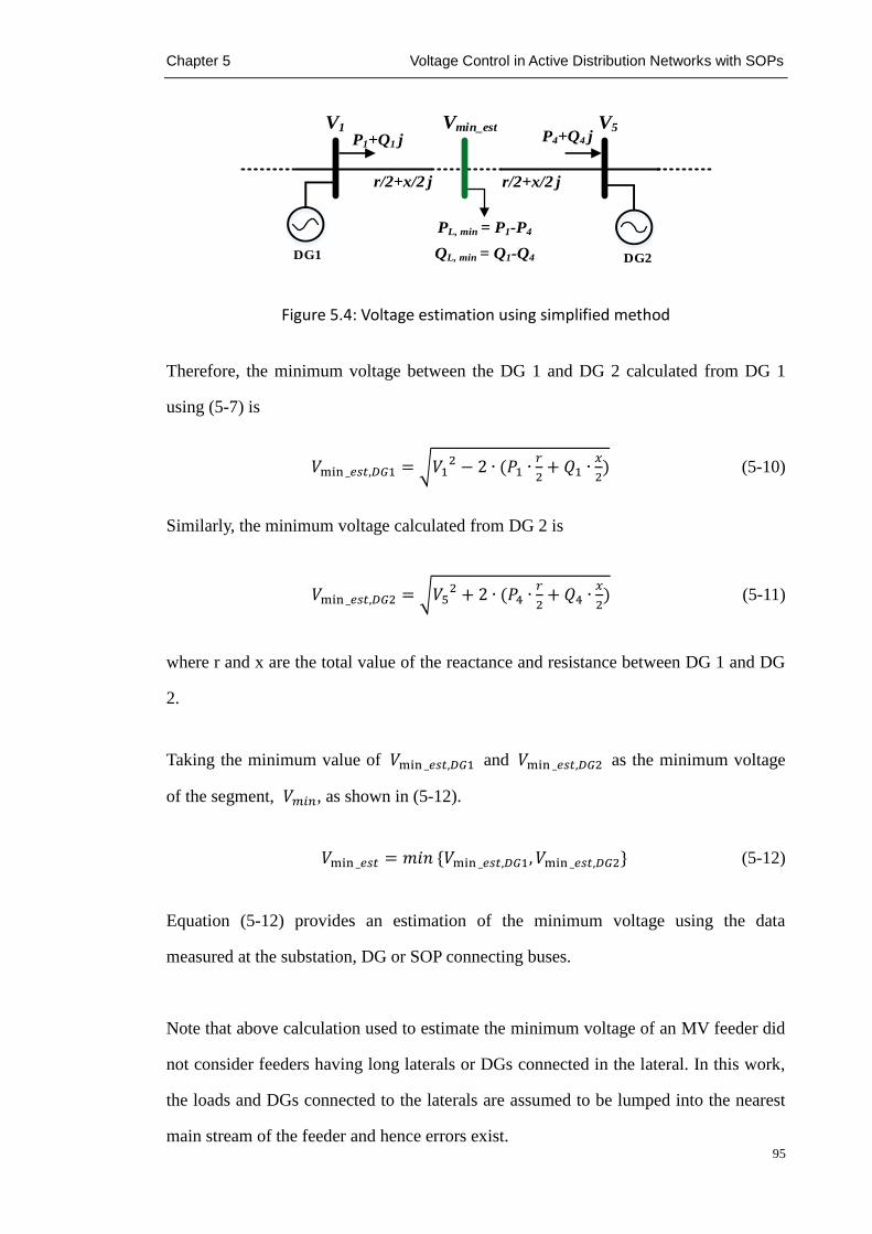
Chapter 5 Voltage Control in Active Distribution Networks with SOPs
95
V1
r/2+x/2 j
P1+Q1 j
DG2DG1
V5Vmin_estP4+Q4 j
r/2+x/2 j
PL, min = P1-P4
QL, min = Q1-Q4
Figure 5.4: Voltage estimation using simplified method
Therefore, the minimum voltage between the DG 1 and DG 2 calculated from DG 1
using (5-7) is
𝑉min _𝑒𝑠𝑡,𝐷𝐺1 = √𝑉12 − 2 ∙ (𝑃1 ∙
𝑟
2+ 𝑄1 ∙
𝑥
2) (5-10)
Similarly, the minimum voltage calculated from DG 2 is
𝑉min _𝑒𝑠𝑡,𝐷𝐺2 = √𝑉52 + 2 ∙ (𝑃4 ∙
𝑟
2+ 𝑄4 ∙
𝑥
2) (5-11)
where r and x are the total value of the reactance and resistance between DG 1 and DG
2.
Taking the minimum value of 𝑉min _𝑒𝑠𝑡,𝐷𝐺1 and 𝑉min _𝑒𝑠𝑡,𝐷𝐺2 as the minimum voltage
of the segment, 𝑉𝑚𝑖𝑛, as shown in (5-12).
𝑉min _𝑒𝑠𝑡 = 𝑚𝑖𝑛 {𝑉min _𝑒𝑠𝑡,𝐷𝐺1, 𝑉min _𝑒𝑠𝑡,𝐷𝐺2} (5-12)
Equation (5-12) provides an estimation of the minimum voltage using the data
measured at the substation, DG or SOP connecting buses.
Note that above calculation used to estimate the minimum voltage of an MV feeder did
not consider feeders having long laterals or DGs connected in the lateral. In this work,
the loads and DGs connected to the laterals are assumed to be lumped into the nearest
main stream of the feeder and hence errors exist.

Chapter 5 Voltage Control in Active Distribution Networks with SOPs
96
5.2.2 Proposed Voltage Control Framework
A distributed voltage control framework is proposed, as depicted in Figure 5.5. Each of
the controllable elements, i.e. the OLTC, the SOP and DG units, is considered as a local
control agent that operates based on the local measurements and the shared data
through an information-sharing platform.
DG
DG DG SOPOLTC
OLTC
AgentDG
Agent
SOP
Agent
Information-sharing Platform
Communication links
Meters
Figure 5.5: Distributed voltage control framework
Local control agents
The local control agents carry out real-time control based on the local measurements
but considering coordination with other local control agents via the information
exchange through the information-sharing platform. Figure 5.6 shows the interior
structure of each control agent.

Chapter 5 Voltage Control in Active Distribution Networks with SOPs
97
Voltage estimation
module
Control algorithm
module
Knowledge base
Bidirectional interface
Local meters Actuators
Information-
sharing platform
Action
Figure 5.6: Interior structure of a local control agent
Details of the four blue blocks shown in Figure 5.6 are given as follows.
Bidirectional interface is responsible for 1) exchanging data with the
information-sharing platform, 2) passing the measurements from the local meters and
the information-sharing platform to the voltage estimation module inside the agent, and
3) passing the control commands issued by the control algorithm module to the
actuator.
Voltage estimation module is responsible for performing the segment voltage
estimation as described in 5.2.1. The detailed process is shown as follows.
1) The module receives the measurements from the local meter. Figure 5.7 shows a
detailed view of the measurements by each local meter. It includes the voltage
magnitude at the connecting bus, the real and reactive power flow in lines
connected to the connecting bus. These measurements provide the measured
potential maximum voltage and the data needed to estimate the minimum
voltages within its corresponding segments, i.e., segments in between its agent
and any neighbour agent.
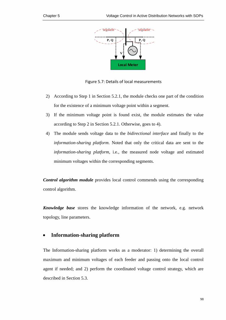
Chapter 5 Voltage Control in Active Distribution Networks with SOPs
98
V
P, Q P, Q
Local Meter
segmentsegment
Figure 5.7: Details of local measurements
2) According to Step 1 in Section 5.2.1, the module checks one part of the condition
for the existence of a minimum voltage point within a segment.
3) If the minimum voltage point is found exist, the module estimates the value
according to Step 2 in Section 5.2.1. Otherwise, goes to 4).
4) The module sends voltage data to the bidirectional interface and finally to the
information-sharing platform. Noted that only the critical data are sent to the
information-sharing platform, i.e., the measured node voltage and estimated
minimum voltages within the corresponding segments.
Control algorithm module provides local control commends using the corresponding
control algorithm.
Knowledge base stores the knowledge information of the network, e.g. network
topology, line parameters.
Information-sharing platform
The Information-sharing platform works as a moderator: 1) determining the overall
maximum and minimum voltages of each feeder and passing onto the local control
agent if needed; and 2) perform the coordinated voltage control strategy, which are
described in Section 5.3.

Chapter 5 Voltage Control in Active Distribution Networks with SOPs
99
5.3 Coordinated Voltage Control Strategy
In this section, the voltage control using the SOP and its coordination with other control
devices (i.e., OLTC and DG units) were investigated. The effectiveness of the SOP on
voltage control and its impacts on networks was first examined. Then, a priority-based
coordination using the proposed control framework described in Section 5.2 was
developed.
5.3.1 Effectiveness of SOP on Voltage Control
Voltage change caused by an SOP
Figure 5.8 shows a radial feeder of an MV network.
V0 Vi-1 Vi Vn
PL,i+QL,i j
ri+xi j
Vi+1
ri-1+xi-1 j
Pi+Qi jPi-1+Qi-1 j Pn+Qn j
Figure 5.8: Radial distribution feeder
According to (5-5)-(5-7), the active and reactive power at node i and the voltage
magnitude at node i can be given as follows:
𝑃𝑖 = 𝑃𝑛 + ∑ 𝑃𝐿,𝑘𝑛𝑘=𝑖+1 (5-13)
𝑄𝑖 = 𝑄𝑛 + ∑ 𝑄𝐿,𝑘𝑛𝑘=𝑖+1 (5-14)
𝑉𝑖2 = 𝑉0
2 − 2 ∙ ∑ (𝑟𝑘𝑃𝑘 + 𝑥𝑘𝑄𝑘)𝑖−1𝑘=0 (5-15)
Equations (5-13) to (5-15) show the change of the branch power flow and consequently
the change of the voltage magnitude at bus i depends on the sum of power loads
(𝑃𝐿,𝑘 and 𝑄𝐿,𝑘), the downstream active and reactive power flow (𝑃𝑛 and 𝑄𝑛) and the

Chapter 5 Voltage Control in Active Distribution Networks with SOPs
100
voltage magnitude at the initial upstream bus (𝑉0), i.e. the substation busbar.
Therefore, if an SOP is connected in the downstream of bus i. According to the generic
power injection model of SOP developed in Chapter 3, the change of the branch power
at bus i caused by the change of the power injection,∆𝑃𝑆_𝑖𝑛𝑗 and ∆𝑄𝑆_𝑖𝑛𝑗 at the SOP
connecting bus can be estimated based on (5-13) and (5-14):
∆𝑃𝑖 = 𝑃𝑖𝑛𝑒𝑤 − 𝑃𝑖
𝑜𝑙𝑑 = ∆𝑃𝑛 = ∆𝑃𝑆_𝑖𝑛𝑗 (5-16)
∆𝑄𝑖 = 𝑄𝑖𝑛𝑒𝑤 − 𝑄𝑖
𝑜𝑙𝑑 = ∆𝑄𝑛 = ∆𝑄𝑆_𝑖𝑛𝑗 (5-17)
Thus, the estimation on the change of the voltage magnitude at bus i using (5-15) can
be obtained as
∆(𝑉𝑖2) = 𝑉𝑖
𝑛𝑒𝑤2−𝑉𝑖
𝑜𝑙𝑑2= (𝑉0
𝑛𝑒𝑤2−𝑉0
𝑜𝑙𝑑2) − 2 ∙ ∑ 𝑟𝑘 ∙ ∆𝑃𝑆𝑖𝑛𝑗
𝑖−1𝑘=0 − 2 ∙ ∑ 𝑥𝑘 ∙ ∆𝑄𝑆𝑖𝑛𝑗
𝑖−1𝑘=0
= ∆(𝑉02) − 2 ∙ ∑ 𝑟𝑘 ∙ ∆𝑃𝑆𝑖𝑛𝑗
𝑖−1𝑘=0 − 2 ∙ ∑ 𝑥𝑘 ∙ ∆𝑄𝑆𝑖𝑛𝑗
𝑖−1𝑘=0 (5-18)
where ∆(𝑉02) is the change of the substation voltage; 2 ∙ ∑ 𝑟𝑘
𝑖−1𝑘=0 and 2 ∙ ∑ 𝑥𝑘
𝑖−1𝑘=0
are the sensitivity factors of bus i. These sensitivity factors constants determined by the
line parameters only.
While, for bus i in the downstream of SOP connecting bus, the change of the voltage at
bus i equals to the change of the voltage at the SOP connecting bus j, which is written
as follows:
∆(𝑉𝑖2) = ∆(𝑉0
2) − 2 ∙ ∑ 𝑟𝑘 ∙ ∆𝑃𝑆_𝑖𝑛𝑗𝑗𝑘=0 − 2 ∙ ∑ 𝑥𝑘 ∙ ∆𝑄𝑆_𝑖𝑛𝑗
𝑗𝑘=0 (5-19)
Note that the change of the substation voltage, i.e., ∆(𝑉02) is calculated based on the
transformer impedance and the system input impedance at the primary side of the
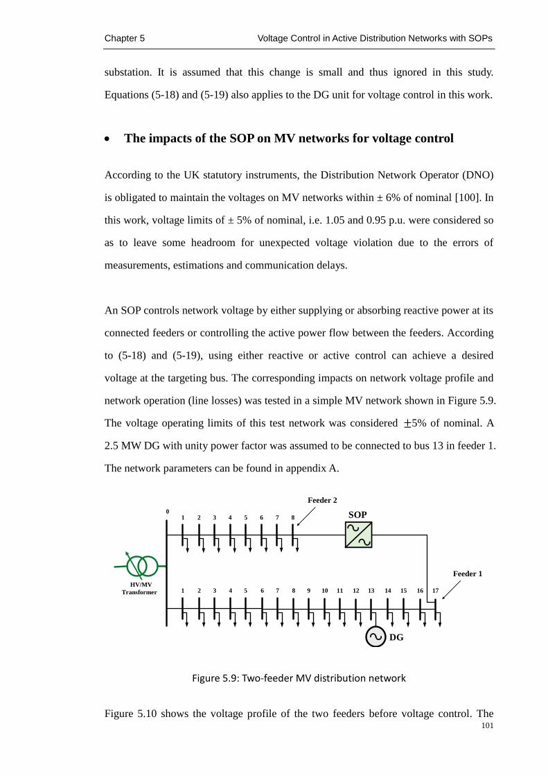
Chapter 5 Voltage Control in Active Distribution Networks with SOPs
101
substation. It is assumed that this change is small and thus ignored in this study.
Equations (5-18) and (5-19) also applies to the DG unit for voltage control in this work.
The impacts of the SOP on MV networks for voltage control
According to the UK statutory instruments, the Distribution Network Operator (DNO)
is obligated to maintain the voltages on MV networks within ± 6% of nominal [100]. In
this work, voltage limits of ± 5% of nominal, i.e. 1.05 and 0.95 p.u. were considered so
as to leave some headroom for unexpected voltage violation due to the errors of
measurements, estimations and communication delays.
An SOP controls network voltage by either supplying or absorbing reactive power at its
connected feeders or controlling the active power flow between the feeders. According
to (5-18) and (5-19), using either reactive or active control can achieve a desired
voltage at the targeting bus. The corresponding impacts on network voltage profile and
network operation (line losses) was tested in a simple MV network shown in Figure 5.9.
The voltage operating limits of this test network was considered ±5% of nominal. A
2.5 MW DG with unity power factor was assumed to be connected to bus 13 in feeder 1.
The network parameters can be found in appendix A.
1 2 3 4 5 6 7 8 9 10 11 12 13 14 15 16 17
01 2 3 4 5 6 7 8
HV/MV
Transformer
DG
SOP
Feeder 2
Feeder 1
Figure 5.9: Two-feeder MV distribution network
Figure 5.10 shows the voltage profile of the two feeders before voltage control. The

Chapter 5 Voltage Control in Active Distribution Networks with SOPs
102
voltages from bus 12 down to bus 17 violated the upper limit due to the DG connection,
while the minimum voltage (on the other feeder) approached to the lower limit. The
OLTC is infeasible for voltage control in such a case since the difference between the
overall maximum and minimum voltages exceeded the gap between the upper and
lower voltage limits and thus may cause improper settings and excessive tap operation
[101]. Therefore, the SOP was used to reduce the voltages in feeder 1 by controlling
either real or reactive power based on equation (5-18).
Figure 5.10: Voltage profiles of both feeder before voltage control
According to (5-18), it was assumed that the target bus is 13 and the desired voltage
magnitude at the target bus, 𝑉13𝑛𝑒𝑤 was set to be 1 p.u. Figure 5.11 shows the voltage
profile with SOP control using different control methods. It is observed that both
control methods achieved the control task, i.e., the voltages at bus 13 were close to the
targeted value (1 p.u.).For active power control shown in Figure 5.11a, the voltage
profile along feeder 2 rose while the voltage profile along feeder 1 dropped. This is due
to the active power was transferred from feeder 1 to feeder 2. However, for the reactive
control method, the reactive power was controlled independently on either side of the
SOP and thus the voltage profile along the feeder 2 was not changed. In addition, it is
shown that the closer to the SOP connecting bus, the bigger the increased (or decreased)
voltage magnitude.. This can be explained by (5-19) where the sensitivity factors, 2 ∙
0.95
0.975
1
1.025
1.05
1.075
0 1 2 3 4 5 6 7 8 9 10 11 12 13 14 15 16 17
Volt
age
(p.u
.)
Bus Number
Feeder 1 Feeder 2
Upper limit
Lower limit

Chapter 5 Voltage Control in Active Distribution Networks with SOPs
103
∑ 𝑟𝑘𝑖−1𝑘=0 and 2 ∙ ∑ 𝑥𝑘
𝑖−1𝑘=0 increase with the distance between bus i and the substation
bus increases.
(a)
(b)
Figure 5.11: Voltage profiles with SOP voltage control: (a) active power control method;
(b) reactive power control method
Figure 5.12 compares the network power losses before and after using SOP control.
There was a significant increase of network power losses after using the reactive power
control method. This is because the voltage improvement was achieved by absorbing
excessive reactive power from the network, which caused an increased in feeder
loading and consequently an increase in the line losses. On the contrary, the network
power losses were decreased by using the active power control method which
transferred active power between feeder 1 and feeder 2.
0.95
0.975
1
1.025
1.05
0 1 2 3 4 5 6 7 8 9 10 11 12 13 14 15 16 17
Vo
ltag
e (p
.u.)
Bus Number
SOP_P control - feeder 1
SOP_P control - feeder 2
0.925
0.95
0.975
1
1.025
1.05
0 1 2 3 4 5 6 7 8 9 10 11 12 13 14 15 16 17
Volt
age
(p.u
.)
Bus Number
SOP_Q control - feeder 1
SOP_Q control - feeder 2

Chapter 5 Voltage Control in Active Distribution Networks with SOPs
104
Figure 5.12: Comparison of the network active power losses
Discussion
According to the above analysis, the following key findings of the SOP control are
outlined:
Either real or reactive power control of the SOP achieves the voltage control
objective by using the sensitivity factors in (5-18). However, the voltage change
is more sensitive to the active power control due to the fact that MV distribution
networks have high line resistances and low X/R ratio [102]. This makes the
active power control method more cost-effective considering the device capacity.
For active power control method, the voltage profile on both feeders will be
affected. A decrease in the voltage profile on one feeder leads to an increase in
the voltage on the other feeder, and vice versa. Therefore, the voltage headroom
of both connected feeders need to be considered when the active power control
method is used. The main advantage of this control method compared with the
reactive power control is that there will not be a significant change on network
power losses using the active power control.
The main advantage of the reactive power control method is that both sides of
SOP supply and/or absorb reactive power independently. Therefore, it enables
voltage control simultaneously and independently on both connected feeders.
However, the voltage drop by absorbing excessive reactive power may cause a
165.1452
101.158
434.5934
0
100
200
300
400
500
Original SOP_P control SOP_Q control
To
tal
po
wer
lo
ss (
kW
)

Chapter 5 Voltage Control in Active Distribution Networks with SOPs
105
significant increase in network power losses.
5.3.2 Priority-Based Coordination
Figure 5.13 shows a priority-based coordination among multiple agents, including the
OLTC, the SOP and the DG units. Each of these agents is called a “local control agent”
and each local control agent has multiple objectives. The first one (main objective) is
identical to all agents and the remaining are called sub-objectives. The main objective
used in this work is to keep the voltages within the allowable range. The sub-objectives
are to reduce the number of tap operations, mitigate DG active power curtailment, and
reduce network power losses.
OLTC
Agent
DG
Agent
SOP
Agent
Information-sharing
Platform
No voltage violations
Less active power curtailment
Fewer network power losses
No voltage violations
Fewer number of tap operations
No voltage violations
Fewer network power losses
Exchange
messages
Exchange
messages
Exchange
messages
Figure 5.13: Priority-based coordination of the multiple local control agents
In order to achieve a trade-off among the aforementioned objectives, the objectives
were grouped by defining the priority level, as shown in Figure 5.14.

Chapter 5 Voltage Control in Active Distribution Networks with SOPs
106
No voltage violation
Less tap operation
Fewer network power losses
Maximize energy capture
Priority LevelH
L
Figure 5.14: Prioritisation of the proposed objectives from high (H) to low (L)
A priority-based coordination is carried out to allow the local control agents to achieve
their objectives in accordance with a specific sequence (i.e., the prioritisation). Figure
5.15 shows the flow chart of the priority-based coordination. Both DG and SOP control
agents have two voltage control methods: real and reactive power control methods. The
OLTC agent also has two control strategies to deal with both feasible and infeasible
solutions. The main objective (no voltage violation) is considered each time before a
control method to determine whether a control action is needed. All the control
methods are coordinated in a pre-defined sequence based on the prioritisation of the
sub-objectives. The higher the priority level, the later the corresponding control method
will be activated.
Thus, as shown in the figure 5.15, the real and reactive power control of the SOP and
the reactive control of the DG (green block) are the first considered methods. They are
activated in a sequence that: 1) the active power control of the SOP agent is prior to the
reactive power control methods due to the results obtained from Section 5.3.1, i.e., the
active power control method is more sensitive to voltage change and results in reduced
network power losses and 2) the reactive control method of the SOP agent is prior to
that of the DG agent in order to allow more flexibility for the DG unit in case of an
emergency [56]. All these real and reactive control methods are performed by solving
an optimization problem to minimize the voltage deviation, and thus, reduce the
number of tap operations. The second activated method is the OLTC control (yellow
block). A double-check process (grey block) is introduced before activating the last
control method in order to ensure that there is no feasible solutions to enable an OLTC

Chapter 5 Voltage Control in Active Distribution Networks with SOPs
107
control (feasible solution strategy). The last activated control method is the active
power curtailment by the DG, as the brown block shown.
Start
SOP_Real power control method
Voltage violation?
SOP_Reactive power control method
Voltage violation?
DG_Reactive power control method
Feasible solution?
Stop double check ?
OLTC_Feasible
solution strategyEnd
OLTC_Infeasible solution strategy
DG_Real power curtailment
Voltage violation?
Yes
Yes
Yes
Yes
Yes No
No
No
No
Less network power losses
Less tap operation
Maximize energy capture
Double check processNo
Voltage violation?No
Yes
Double check
process
Voltage violation?No
Yes
Figure 5.15: Flow chart of the proposed priority-based coordination
The details of the voltage control method for each agent and the double check process
are given as follows.

Chapter 5 Voltage Control in Active Distribution Networks with SOPs
108
Voltage control for the SOP agent
A. Bidirectional interface
The SOP control agent receives data from the information-sharing platform. These data
contains the action command, magnitudes and locations of all potential maximum and
minimum voltages along the connected feeders. The action command specifies the
method to be activated at current time step. The locations of all potential maximum and
minimum voltage points are sent to the knowledge based to calculate the sensitivity
factors.
After the control algorithm module determines the required real or reactive power for
the SOP agent, two messages are sent out via the interface: the new real or reactive
power set point to the actuator and the action confirmed message to the
information-sharing platform.
B. Control algorithm module
The control algorithm module implements the control algorithm based on the action
command, voltage data and the corresponding sensitivity factors.
1) Active power control algorithm
The active power control algorithm solves the optimization problem shown in
(5-20)-(5-23). The objective function aims to minimize the voltage deviation of the
maximum and minimum voltages along both connected feeders from the nominal value,
𝑉𝑛𝑜𝑟𝑚:
Minimize 𝐹(𝑃𝑆_𝑖𝑛𝑗𝑛𝑒𝑤 ) = ∑ (𝑉𝑖 − 𝑉𝑛𝑜𝑟𝑚)2𝑁
𝑖=1 (5-20)
subject to
|𝑃𝑆_𝑖𝑛𝑗𝑛𝑒𝑤 | ≤ 𝑃𝑆_𝑖𝑛𝑗
𝑙𝑖𝑚 , 𝑃𝑆_𝑖𝑛𝑗𝑙𝑖𝑚 = √𝑆𝑆𝑂𝑃
𝑟𝑎𝑡𝑒2− 𝑄𝑆_𝑖𝑛𝑗
2 (5-21)

Chapter 5 Voltage Control in Active Distribution Networks with SOPs
109
𝑉𝑖𝑛𝑒𝑤2
= 𝑉𝑖𝑜𝑙𝑑2
− 𝑀𝑖 ∙ (𝑃𝑆_𝑖𝑛𝑗𝑛𝑒𝑤 − 𝑃𝑆_𝑖𝑛𝑗
𝑜𝑙𝑑 ) (5-22)
𝑉𝑚𝑖𝑛𝑏𝑎𝑛𝑑 ≤ 𝑉𝑖 ≤ 𝑉𝑚𝑎𝑥
𝑏𝑎𝑛𝑑 (5-23)
where 𝑉𝑖 is the voltage magnitude received from the interface; N is the total number of
voltage points received from the interface; 𝑆𝑆𝑂𝑃𝑙𝑖𝑚 is the rating power of the SOP device;
𝑀𝑖 is the sensitivity factor for the change of voltage 𝑉𝑖 with respect to the change of
active power; 𝑉𝑚𝑖𝑛𝑏𝑎𝑛𝑑 and 𝑉𝑚𝑎𝑥
𝑏𝑎𝑛𝑑 are the acceptable limits of bandwidth for voltage
control using the SOP agent. In this work, 𝑉𝑛𝑜𝑟𝑚 is assumed to be 1 p.u., i.e., a middle
point between the upper and lower limits in order to leave headroom for both over- and
under-voltage issues due to the future DG penetrations and increase of demands, e.g.,
electric vehicles and heat pumps.
Note that the defined bandwidth in (5-23) is wider than the specified limits to avoid the
infeasible solution, which may occur due to the device power limits in (5-21). This
wider bandwidth is also applied to the reactive power method of the SOP and DG agent
and is refined by using the OLTC agent to ensure that the network voltages within the
statutory limits. The optimization algorithm used in this study was the Powell’s Direct
Set Method, which is described in Chapter 4.
2) Reactive power control algorithm
The aim of reactive power control is to minimize the voltage deviation from the
nominal value and the amount of reactive power absorbed by the SOP to improve
voltage control. The objective function is defined as
Minimize 𝐽 (𝑄𝑆𝑖𝑛𝑗
𝑛𝑒𝑤) = ∑ (𝑉𝑖 − 𝑉𝑛𝑜𝑟𝑚)2𝑁𝑖=1 − 𝜔𝑎𝑏𝑠𝑜𝑟 ∙ 𝑚𝑖𝑛{0, 𝑄𝑆𝑖𝑛𝑗
𝑛𝑒𝑤} (5-24)
subject to

Chapter 5 Voltage Control in Active Distribution Networks with SOPs
110
|𝑄𝑆𝑖𝑛𝑗
𝑛𝑒𝑤| ≤ 𝑄𝑆_𝑖𝑛𝑗𝑙𝑖𝑚 , 𝑄𝑆_𝑖𝑛𝑗
𝑙𝑖𝑚 = √𝑆𝑆𝑂𝑃𝑙𝑖𝑚 2
− 𝑃𝑆_𝑖𝑛𝑗2 (5-25)
𝑉𝑖𝑛𝑒𝑤2
= 𝑉𝑖𝑜𝑙𝑑2
− 𝐾𝑖 ∙ (𝑄𝑆_𝑖𝑛𝑗𝑛𝑒𝑤 − 𝑄𝑆_𝑖𝑛𝑗
𝑜𝑙𝑑 ) (5-26)
𝑉𝑚𝑖𝑛𝑏𝑎𝑛𝑑 ≤ 𝑉𝑖 ≤ 𝑉𝑚𝑎𝑥
𝑏𝑎𝑛𝑑 (5-27)
where 𝑄𝑆𝑖𝑛𝑗
𝑛𝑒𝑤 is the reactive power supplied by the SOP, and it turns to be a negative
value when the SOP absorbs reactive power from the connected feeder; 𝜔𝑎𝑏𝑠𝑜𝑟 is the
penalty factor for absorbing reactive power from the connected feeder in order to avoid
the increase in the losses along the feeder, i.e., the term −𝜔𝑎𝑏𝑠𝑜𝑟 ∙ 𝑚𝑖𝑛{0, 𝑄𝑆𝑖𝑛𝑗
𝑛𝑒𝑤} will
turn to be a non-zero (positive) value and add to the objective function when the SOP
absorbs reactive power from the network; 𝐾𝑖 is the sensitivity factor for the change of
voltage 𝑉𝑖 with respect to the change of reactive power.
Voltage control for the DG agent
In this work, the DG units are assumed to operate at the maximum power point tracking
(MPPT) before receiving the voltage control command from the information-sharing
platform. Once receiving a command, the DG agents will accept or refuse the command
based on the assessment of the request, for instance, assessing the remaining capacity
for voltage support.
A. Bidirectional interface
The DG agent receives data from the information-sharing platform. Similar to the SOP
agent, these data contains the action command, magnitudes and locations of potential
maximum and minimum voltages along the connected feeder. The action command
specifies the control method to be activated at current time step, i.e., reactive power
control or active power curtailment. The locations of potential maximum and minimum
voltage points are sent to the knowledge based to calculate the sensitivity factors.

Chapter 5 Voltage Control in Active Distribution Networks with SOPs
111
After the control algorithm module determines the required reactive power or active
power curtailment from the DG agent, two messages are sent out via the interface: the
new power set point to the actuator and the action confirmed message to the
information-sharing platform
B. Control algorithm module
1) Reactive power control algorithm
The aim of reactive power control by the DG agent is similar to that of the SOP agent.
The objective function is given as
Minimize 𝐽(𝑄𝑔𝑛𝑒𝑤) = ∑ (𝑉𝑖 − 𝑉𝑛𝑜𝑟𝑚)2𝑁
𝑖=1 + 𝜔𝑎𝑏𝑠𝑜𝑟 ∙ 𝑚𝑖𝑛{0, 𝑄𝑔𝑛𝑒𝑤} (5-28)
subject to
|𝑄𝑔𝑛𝑒𝑤| ≤ 𝑄𝑆_𝑖𝑛𝑗
𝑙𝑖𝑚 , 𝑄𝑆_𝑖𝑛𝑗𝑙𝑖𝑚 = √𝑆𝑔
𝑟𝑎𝑡𝑒2− 𝑃𝑔
2 (5-29)
𝑉𝑖𝑛𝑒𝑤2
= 𝑉𝑖𝑜𝑙𝑑2
− 𝐾𝑖 ∙ (𝑄𝑔𝑛𝑒𝑤 − 𝑄𝑔
𝑜𝑙𝑑) (5-30)
𝑉𝑚𝑖𝑛𝑏𝑎𝑛𝑑 ≤ 𝑉𝑖 ≤ 𝑉𝑚𝑎𝑥
𝑏𝑎𝑛𝑑 (5-31)
where 𝑄𝑔𝑛𝑒𝑤 is the reactive power supplied by the SOP, and it turns to be a negative
value when the DG absorbs reactive power from the connected feeder; 𝜔𝑎𝑏𝑠𝑜𝑟 is the
weight for absorbing reactive power from the connected feeder; 𝐾𝑖 is the sensitivity
factor for the change of voltage 𝑉𝑖 with respect to the change of reactive power.
2) Active power curtailment algorithm
The objective of this method is to determine the required active power curtailment that
keeps the maximum voltage within the specified upper limits using
𝑉𝑈𝑝𝑝𝑒𝑟2 − 𝑉𝑚𝑎𝑥
𝑜𝑙𝑑 2+ 𝑀𝑚𝑎𝑥 ∙ (𝑃𝑔
𝑛𝑒𝑤 − 𝑃𝑔𝑀𝑃𝑃𝑇) =0 (5-32)
Chapter 5 Voltage Control in Active Distribution Networks with SOPs
112
where 𝑀𝑚𝑎𝑥 is the sensitivity factor of the maximum voltage point; 𝑃𝑔𝑀𝑃𝑃𝑇 is the
active power generation of the DG units under MPPT mode.
C. Coordination among multiple DG agents
The aim of coordinating multiple DG agents for voltage control is to minimize the cost
of reactive power control and active power curtailment for all participated DG agents.
In this work, all DG agents are assumed to have equal weights of real and reactive
power control for voltage control. Therefore, the cost is only determined by the amount
of reactive power support or active power curtailment of the participated DG agents.
The coordination schemes among DG agents for different control methods are
summarized as follows.
1) Coordination for reactive power control
A prioritization of the DG agents for reactive power control is determined based on the
sensitivity factors using the follows steps:
Step 1) If the information–sharing platform determines to activate the reactive
power control from DG agents, the last downstream DG along the feeder
(most sensitive to voltage change) is informed first to achieve the
optimization purpose. The required reactive power is calculated using
(5-28) and the new reference is updated.
Step 2) If there is still voltage violations after activating the last downstream DG
agent, the next upstream DG agent (second most sensitive to voltage
change) is activated.
Step 3) Step 1) and 2) are repeated until there is no voltage violation along the
feeder or the fist upstream DG agent is reached.
2) Coordination for active power curtailment
For active power control, the DG agent where the connecting bus has an overvoltage is
activated first. The next downstream DG agent is activated if there is still a voltage
violation. This sequence is due to the factors that 1) any DG agent connecting to the

Chapter 5 Voltage Control in Active Distribution Networks with SOPs
113
downstream feeder of the overvoltage bus has the same while maximum sensitivity
factor to the overvoltage bus; and 2) the further the downstream DG is to the
substation, the more sensitive to voltage change it will be thus has a higher possibility
to cause the voltage at any other bus exceeding the lower limit due to the active power
curtailment.
Voltage control for the OLTC agent
It was assumed in this study that the substation transformer has an on-load tap changer
on the primary winding and the voltage on the primary side remains constant.
A. Bidirectional interface
The OLTC agent receives the action command and the overall maximum and minimum
voltages of the network from the information-sharing platform. The action command
specifies the control strategy required: feasible solution strategy or infeasible solution
strategy. After the control algorithm module determines the new tap setting of the
OLTC agent, two messages are sent out via the interface: the new reference to the
actuator and the task confirmed message to the information-sharing platform
B. Control algorithm module
The control algorithm module receives the voltage data and action command from the
interface and then implements the relevant control strategy described below.
1) Feasible solution strategy
When the agent receives a feasible solution message, i.e., 𝑉𝑚𝑎𝑥 − 𝑉𝑚𝑖𝑛 ≤ 𝑉𝑢𝑝𝑝𝑒𝑟 −
𝑉𝑙𝑜𝑤𝑒𝑟, the control algorithm module calculates the number of required taps at each
time step i using
{𝑇𝑖 = 𝑇𝑖−1 + round (
𝑉𝑚𝑖𝑛−𝑉𝑙𝑜𝑤𝑒𝑟
∆𝑉) , if 𝑉𝑙𝑜𝑤𝑒𝑟 > 𝑉𝑚𝑖𝑛
𝑇𝑖 = 𝑇𝑖−1 + round (𝑉𝑢𝑝𝑝𝑒𝑟 − 𝑉𝑚𝑎𝑥
∆𝑉) , if 𝑉𝑢𝑝𝑝𝑒𝑟 < 𝑉𝑚𝑎𝑥
(5-33)
Chapter 5 Voltage Control in Active Distribution Networks with SOPs
114
subject to
𝑉𝑠 = 𝑉𝑝 + 𝑇 ∙ ∆𝑉 (5-34)
𝑇upp𝑒𝑟 ≤ 𝑇𝑖 ≤ 𝑇Lower (5-35)
Where 𝑇𝑖 and 𝑇𝑖−1 is the tap position at time step i and i-1; 𝑉𝑚𝑎𝑥 and 𝑉𝑚𝑖𝑛 are the
overall maximum and minimum voltage of the network; 𝑉𝑢𝑝𝑝𝑒𝑟 and 𝑉𝑙𝑜𝑤𝑒𝑟 are the
standard upper and lower voltage limits; 𝑇𝑜𝑙𝑑 is current tap position; ∆𝑉 is the step
voltage of each tap; 𝑉𝑠 is the secondary voltage of the substation; 𝑉𝑝 is primary
voltage of the substation; 𝑇upp𝑒𝑟 and 𝑇Lower are the upper and lower boundary of the
OLTC.
2) Infeasible solution strategy
The infeasible solution strategy is required after the double check process while the
infeasible solution still exists. The aim of this strategy is to keep the minimum voltage,
𝑉𝑚𝑖𝑛 at the specified lower limit. Thus the maximum voltage though still violates the
upper limit but is as low as possible, which in turn minimize the required curtailment of
the DG active power. Thus the new tap setting is obtained using
𝑇𝑖 = 𝑇𝑖−1 + round (𝑉𝑚𝑖𝑛−𝑉𝑙𝑜𝑤𝑒𝑟
∆𝑉) (5-36)
subject to
𝑇upp𝑒𝑟 ≤ 𝑇𝑖 ≤ 𝑇Lower (5-37)
Voltage control for the double check process
The purpose of the double check process is to avoid unnecessary DG active power
curtailment. It is achieved by enabling a feasible solution for the OLTC control by
either controlling the violated extreme voltage or controlling the other extreme voltage.
The whole process is performed within the information-sharing platform as follows:
Step 1) Check for the condition of an infeasible solution before activating the
Chapter 5 Voltage Control in Active Distribution Networks with SOPs
115
OLTC agent using
𝑉𝑢𝑝𝑝𝑒𝑟 − 𝑉𝑙𝑜𝑤𝑒𝑟 < 𝑉𝑚𝑎𝑥 − 𝑉𝑚𝑖𝑛 (5-38)
Step 2) If the infeasible solution is raised, allocate the feeders where 𝑉𝑚𝑎𝑥 and
𝑉𝑚𝑖𝑛 happen and then initiate the double check process. Otherwise, send
an action command to the OLTC agent to activate the feasible solution
strategy.
Step 3) If the double check process is initiated, activate the control agent (or
method) that is connected to the feeder where 𝑉𝑚𝑎𝑥 or 𝑉𝑚𝑖𝑛 happens.
The control method that has already been activated is not involved in this
process.
Step 4) If there are multiple candidates, repeat step 1) - 3) until there is a feasible
solution or all the candidates have been activated. The sequence of
activating a candidate at each time step is based on the proposed
coordination law shown in Figure 5.13, i.e., SOP active power control,
SOP reactive control and finally DG reactive power control.
5.3.3 Implementation procedures of the information-sharing platform
The overall implementation procedures of the information-sharing platform are
summarized below.
Step 1) Update the voltage information after receiving segment voltage data from
the local control agents.
Step 2) Determine the maximum and minimum voltages in each feeder. Then,
check the condition of voltage violation.
Step 3) If there is no voltage violation, go to step 1. Otherwise, allocate the
feeders at which the voltage exceeds the specified limit and then initiate
the coordinated control on these feeders.
Step 4) Send an action command to activate the relevant agent based on the

Chapter 5 Voltage Control in Active Distribution Networks with SOPs
116
coordination law described in Section 5.3.2.
Step 5) Each time after receiving the action confirmed message from the agent,
update voltage information by repeating step 1) and 2). If there is no
voltage violation or all available control methods have been activated, go
to step 1). Otherwise, go to step 4).
5.4 Discussion: Benefits of the Proposed Control
Strategy
The main advantages of the coordinated voltage control strategy are summarized
below.
The proposed voltage control framework allows for required coordination
between multiple agents (devices) while independent real-time control by each
local control agent. Moreover, it is easy to modify and upgrade each local
control agent or implement expansion (e.g. more DG connections) without
interrupting other parts of control framework.
Further flexibility is provided by the SOP when the over- and under-voltage
issues exist simultaneously within a network that cannot be solved by the OLTC.
The use of SOP also reduces network power losses compared to reactive power
control (e.g. capacitor banks). Moreover, the power electronic based device
provides fast enough voltage control compared with the tap changing devices
(e.g., OLTC, capacitor banks), which may be needed for DGs to ride through the
voltage sags during emergency conditions.
A trade-off of the objectives, according to their prioritisation, is achieved by
using the proposed priority-based coordination method. This method performed
by an information-sharing platform is in line with the distributed control
concept while unnecessary negotiation process among agents is eliminated and
data communications are reduced.

Chapter 5 Voltage Control in Active Distribution Networks with SOPs
117
The computational burden is reduced because 1) a distributed voltage control is
achieved by the local control agent, instead of doing a centralised
calculation/optimisation using all data together, and 2) with the use of the
simplified estimation method, the knowledge of the network voltage profile is
obtained by each agent that find their respective maximum voltage and
minimum voltages (within its corresponding segments) simultaneously. In
addition, the numerical convergence problems of running the power flow
algorithm is eliminated since there is no need for running the power flow
algorithm in each time step, especially in the case of high R/X ratio networks.
The communication investments are reduced since the meters and sensors are
placed at the OLTC, DG and SOP connecting points and only the critical data
are exchanged via the information-sharing platform.
5.5 Case Study
The effectiveness of the coordinated voltage control strategy was verified on an MV
distribution network obtained from [55], as shown in Figure 5.16. This network is a
33-bus 11-kV distribution system with four feeders. The four feeders have different
lengths, ratings and load types. Intermittent DG units with different characteristics were
connected to different buses to simulate the unbalance in load/generation diversity
between feeders. Table 5.1 shows a summary of the loads and DGs data. Figure 5.17
depicts the normalized profiles for different load types (commercial, residential and
industrial) and for different DG types within two days (a weekday and a weekend).
These normalized profiles (half-hourly per step) were multiplied by the rated power of
each load or DG (shown in Table 5.1) to have the power daily profile of each bus. All
these data were obtained from [55]. More detailed network data can be found in the
Appendix B. The voltage limits of this test network are 11 kV ±5%. The OLTC was
assumed to have 32 taps with 0.00625 p.u. per step. An SOP was assumed to be
installed between feeder 2 and 3. The capacity limit of the SOP is 1 MVA. This study

Chapter 5 Voltage Control in Active Distribution Networks with SOPs
118
was programmed in Java and C. Balanced three-phase feeders were considered.
SOP
OLTC
1 2 3 4 5 6 7 8 9 10
1 2 3 4 5 6
1 2 3 4 5 6 7 8 9
1 2 3 4 5 6 7 8
Feeder 1
Feeder 2
Feeder 3
Feeder 4
Wind
PV
33 kV/11 kV
Transformer
0
Figure 5.16: The four-feeder MV test network
Table 5.1: Data of the Load and DG
Feeder
number
Load profile DG profile
Types
Total rated
loading
(MVA)
Types
Locations Ratings
(MVA)
1 Commercial 4 Wind 3, 8 2, 0.5
2 Residential 5 PV 2, 5, 10 5, 2, 1
3 Industrial 3 Wind 3, 6 0.5, 2.5
4 Residential 4.5 PV, wind 5, 8 0.5, 0.5
(a) (b)
Figure 5.17: Normalized profiles of a weekend and weekday: (a) loads; (b) DGs
0
0.2
0.4
0.6
0.8
1
No
mal
ized
act
ive
po
wer
(P
g)
Time (hours)
Wind PV
6am 6pm6am 6pm12pm 12pm12am 12am 12am0.3
0.4
0.5
0.6
0.7
0.8
0.9
1
No
min
aliz
ed p
ow
er
Time (hours)
CommertialResidentialIndustrial
6am 6pm6am 6pm12pm 12pm12am 12am 12am

Chapter 5 Voltage Control in Active Distribution Networks with SOPs
119
5.5.1 Voltage Profile Estimation
The voltage profile generated by the estimation method proposed in section 5.2.1 was
compared with the actual voltage profile (calculated by power flow analysis). Figure
5.18 shows the overall maximum and minimum voltages along each feeder during the
studied two days before voltage control. The maximum voltage was read from meters
thus the same. It can be seen that the estimated minimum voltages were close to the
actual values (the maximum difference is 0.004 p.u). For the minimum voltages, lower
voltage bounds were generated by the proposed simplified estimation method (see the
red curves). Therefore, more conservative voltage references will be used for voltage
control using the proposed estimation method.
(a) (b)
0.87
0.895
0.92
0.945
0.97
0.995
1.02
1.045
Vm
axan
d V
min
of
feed
er 2
(p
.u.)
Time (Hour)
V_estimate-Feeder 2
V_actual-Feeder 2
12am 6am 6pm12pm 12am 6am 6pm12pm 12am0.92
0.935
0.95
0.965
0.98
0.995
1.01
1.025
Vm
axan
d V
min
of
feed
er 1
(p
.u.)
Time (Hour)
V_estimate-Feeder 1
V_actual-Feeder 1
12am 6am 6pm12pm 12am 6am 6pm12pm 12am

Chapter 5 Voltage Control in Active Distribution Networks with SOPs
120
(c) (d)
Figure 5.19 shows the snapshot voltage profiles of all buses along each of the four
feeders at 11 am in the first studied day. The voltage profile by the proposed method
were generated by connecting the critical voltage points, i.e., the measured voltages (at
the substation busbar, SOP and DG connecting buses) and the estimated minimum
voltage within each segment using the segment estimation method. It is clear that all
the maximum and minimum voltage points were captured as expected.
(a) (b)
0.955
0.965
0.975
0.985
0.995
1.005
1.015
1.025
1.035
Vm
axan
d V
min
of
feed
er 3
(p
.u.)
Time (Hour)
V_estimated-Feeder 3V_actual-Feeder 3
12am 6am 6pm12pm 12am 6am 6pm12pm 12am0.9
0.91
0.92
0.93
0.94
0.95
0.96
0.97
0.98
0.99
1
Vm
axan
d V
min
of
feed
er 4
(p
.u.)
Time (Hour)
V_estimate-Feeder 4V_actual-Feeder 4
12am 6am 6pm12pm 12am 6am 6pm12pm 12am
Figure 5.18: Per unit maximum and minimum voltage profile over the studied period
at (a) feeder 1; (b) feeder 2; (c) feeder 3; (d) feeder 4
0.985
0.99
0.995
1
1.005
1.01
1.015
1.02
0 1 2 3 4 5 6 7 8
Vo
ltag
e (p
.u.)
Buses of feeder 1
Voltage profile by power flow analysis
Volatge profile by proposed method
0.98
0.985
0.99
0.995
1
1.005
1.01
1.015
1.02
0 1 2 3 4 5 6 7 8 9 10
Vo
ltag
e (p
.u.)
Buses of feeder 2
Voltage profile by power flow analysis
Volatge profile by proposed method

Chapter 5 Voltage Control in Active Distribution Networks with SOPs
121
(c) (d)
5.5.2 Coordinated voltage control using OLTC and SOP
Most utilities prefer DG units to operate close to the unity power factor and do not
allow regulating the voltage actively at the Point of Common Coupling [103]. In this
context, the coordinated control merely considering the OLTC and SOP was conducted
to investigate the performance of the proposed control strategy. All the DG units were
assumed to operate in maximum power point tracking (MPPT) with unity power factor.
Four control schemes were carried out for comparisons:
Scheme I: Voltage control using the OLTC;
Scheme II: Coordinated control between the OLTC and the SOP assuming only
active power control;
Scheme III: Coordinated control between the OLTC and the SOP assuming only
reactive power control;
Scheme IV: Coordinated control between the OLTC and the SOP assuming both real
and reactive power control based on the proposed priority-based
coordination.
0.94
0.95
0.96
0.97
0.98
0.99
1
1.01
1.02
0 1 2 3 4 5 6 7 8 9
Vo
ltag
e (p
.u.)
Buses of feeder 4
Voltage profile by power flow analysis
Volatge profile by proposed method
0.98
0.985
0.99
0.995
1
1.005
1.01
1.015
1.02
0 1 2 3 4 5 6
Vo
ltag
e (p
.u.)
Buses of feeder 3
Voltage profile by power flow analysis
Volatge profile by proposed method
Figure 5.19: Per unit voltage profile at 11am in the first studied day along (a) feeder 1;
(2) feeder 2; (3) feeder 3; (4) feeder 4

Chapter 5 Voltage Control in Active Distribution Networks with SOPs
122
The performance of the control schemes were evaluated in terms of the network voltage
profile, the number of tap operations, total network power losses and the required size
for the SOP to achieve voltage control.
Network voltage profile
Figure 5.20 shows the overall maximum and minimum voltages of the network during
the studied period when different control schemes are used. As shown in the figure, the
network voltage profiles were within the specified limits for most of the time by using
the OLTC, i.e., Scheme I. However, it could not solve the areas of infeasible solutions
shown in the figure. These areas of infeasible solutions were mitigated when the SOP
was coordinated with the OLTC, i.e., using Scheme II, III and IV.
Figure 5.20: maximum and minimum voltage profiles at different control schemes
Tap operation
Figure 5.21 compares the number of tap changes during the studies period when
different control schemes are used. As shown in the figure, the number of tap
operations was reduced significantly when the SOP was coordinated with the OLTC,
i.e., using Scheme II, III and IV. The highest reduction was achieved by using Scheme
0.9
0.95
1
1.05
1.1
Vm
axan
d V
min
of
the
net
wo
rk (
p.u
.)
Time (Hours)
Scheme I Scheme II Scheme III Scheme IV
12am 6am 6pm12pm 6pm 12am12pm12am 6am
Infeasible solution Infeasible solution Infeasible solution
upper limit
Lower limit
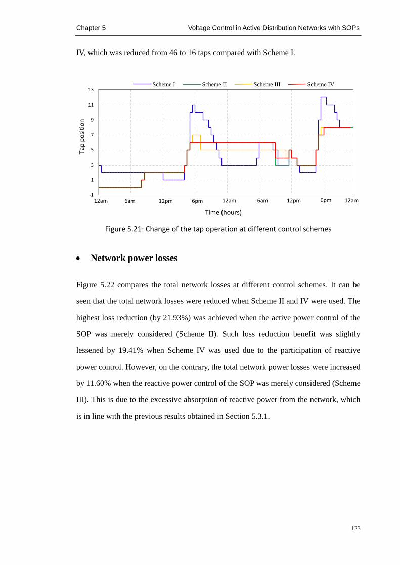
Chapter 5 Voltage Control in Active Distribution Networks with SOPs
123
IV, which was reduced from 46 to 16 taps compared with Scheme I.
Figure 5.21: Change of the tap operation at different control schemes
Network power losses
Figure 5.22 compares the total network losses at different control schemes. It can be
seen that the total network losses were reduced when Scheme II and IV were used. The
highest loss reduction (by 21.93%) was achieved when the active power control of the
SOP was merely considered (Scheme II). Such loss reduction benefit was slightly
lessened by 19.41% when Scheme IV was used due to the participation of reactive
power control. However, on the contrary, the total network power losses were increased
by 11.60% when the reactive power control of the SOP was merely considered (Scheme
III). This is due to the excessive absorption of reactive power from the network, which
is in line with the previous results obtained in Section 5.3.1.
-1
1
3
5
7
9
11
13
Tap
po
siti
on
Time (hours)
Scheme I Scheme II Scheme III Scheme IV
12am 6am 6pm12pm 6pm 12am12pm12am 6am

Chapter 5 Voltage Control in Active Distribution Networks with SOPs
124
Figure 5.22: Total network losses at different control schemes
Required size of the SOP
Figure 5.23 shows the required size (in apparent power) of the SOP for the
corresponding control schemes. All the three control schemes considering SOP
compensate the changes of the load demands and DG productions which, in turn,
reduces the dynamic changes of the voltage profiles and hence the number of tap
operations. However, the SOP operated at its rated power for most of the time when
only controls reactive power (Scheme III). When controls active power (Scheme II), the
SOP operated at its rated power for only a few hours. The total hours, operating at rated
power using the coordinated real and reactive power control (Scheme IV), was in
between the other two.
50
150
250
350
450
550
650
750
850
Tota
l net
wo
rk lo
sses
(kW
)
Time (Hours)
Scheme I Scheme II Scheme III Scheme IV
12am 6am 6pm12pm 6pm 12am12pm12am 6am

Chapter 5 Voltage Control in Active Distribution Networks with SOPs
125
Figure 5.23: Apparent power requirements for different SOP control schemes
From the above results, it is concluded that the coordination between the OLTC and the
SOP is essential when the OLTC is infeasible to solve the voltage problems. In addition,
the proposed priority-based coordination of the OLTC and SOP achieves the best
compromise of the sub-objectives (in accordance with the prioritisation of the
objectives). It enables smaller number of tap operations comparing to the scheme of
only using the active power control and fewer power losses comparing with only using
the reactive power control.
5.5.3 Coordinated voltage control using OLTC, SOP and DG
Increasing the DG penetration in the distribution network brings more difficulties in
controlling network voltages. The previous control using the OLTC and the SOP may
not be able to control the voltage within the specified limits in such a case. Figure 5.24
shows the overall maximum and minimum voltages of the network during the studied
period when the capacity (rated power shown in Table 5.1) of the DG units (connected
in feeder 2) were enlarged by 10%. It is shown that an overvoltage problem still exist
during the peak PV generation when the coordinated control between OLTC and SOP
was used.
0.25
0.5
0.75
1
S so
p (M
VA
)
Time (Hours)
Scheme II Scheme III Scheme IV
12am 6am 6pm12pm 6pm 12am12pm12am 6am

Chapter 5 Voltage Control in Active Distribution Networks with SOPs
126
Figure 5.24: maximum and minimum voltage profiles when increase DG penetration
The coordinated control using the OLTC, SOP and DG units was conducted in this part.
It was assumed that DG units installed at bus 9 in feeder 1, bus 5 in feeder 2, bus 6 in
feeder 3 and bus 8 in feeder 4 were inverter-based DG unit and thus had the reactive
power control capability. All DG owners were obligated to respond to the active power
curtailment request.
Two different cases were carried out for comparison purposes, which are the
coordinated control using OLTC and DG units and the coordinated control using OLTC,
SOP and DG units. The performance of these two cases were evaluated in terms of the
network voltage profile, the total active power generated by DGs, the number of tap
operations, total network power losses and the power settings of the SOP and DG unit.
Network voltage profile and total active power generated by DGs
Figure 5.25 shows the maximum and minimum voltages of the network during the
studied period. It can be seen that the overvoltage problem was solved for both cases
when the DG units were involved in voltage control. However, DG active power
curtailment was required for the case without involving the SOP control, as shown in
0.9
0.95
1
1.05
1.1
Vm
axan
d V
min
of
the
net
wo
rk (
p.u
.)
Time (Hours)
Coordinated control using OLTC and SOP
12am 6am 6pm12pm 6pm 12am12pm12am 6am
Overvoltage
Upper limit
Lower limit

Chapter 5 Voltage Control in Active Distribution Networks with SOPs
127
Figure 5.26. There was no curtailed DG active power when OLTC, SOP and DG units
were coordinated for voltage control.
Figure 5.25: maximum and minimum voltage profiles with increased DG penetration
by coordinated control with and without involving SOP
Figure 5.26: Total active power generated with increased DG penetration by
coordinated control with and without involving SOP
Tap operation
Figure 5.27 compares the number of tap changes during the studied period at different
cases. As shown in the figure, a smaller number of tap operation was required when the
OLTC, SOP and DG units were coordinated. The tap operation was reduced from 21 to
0.9
0.95
1
1.05
1.1
Vm
axan
d V
min
of
the
net
wo
rk (
p.u
.)
Time (Hours)
Coordinated control using OLTC and DGs Coordinated control unsing OLTC, SOP and DGs
12am 6am 6pm12pm 6pm 12am12pm12am 6am
Upper limit
Lower limit
Curtailed energy
Curtailed energy
To
tal
acti
ve
po
wer
(k
W)
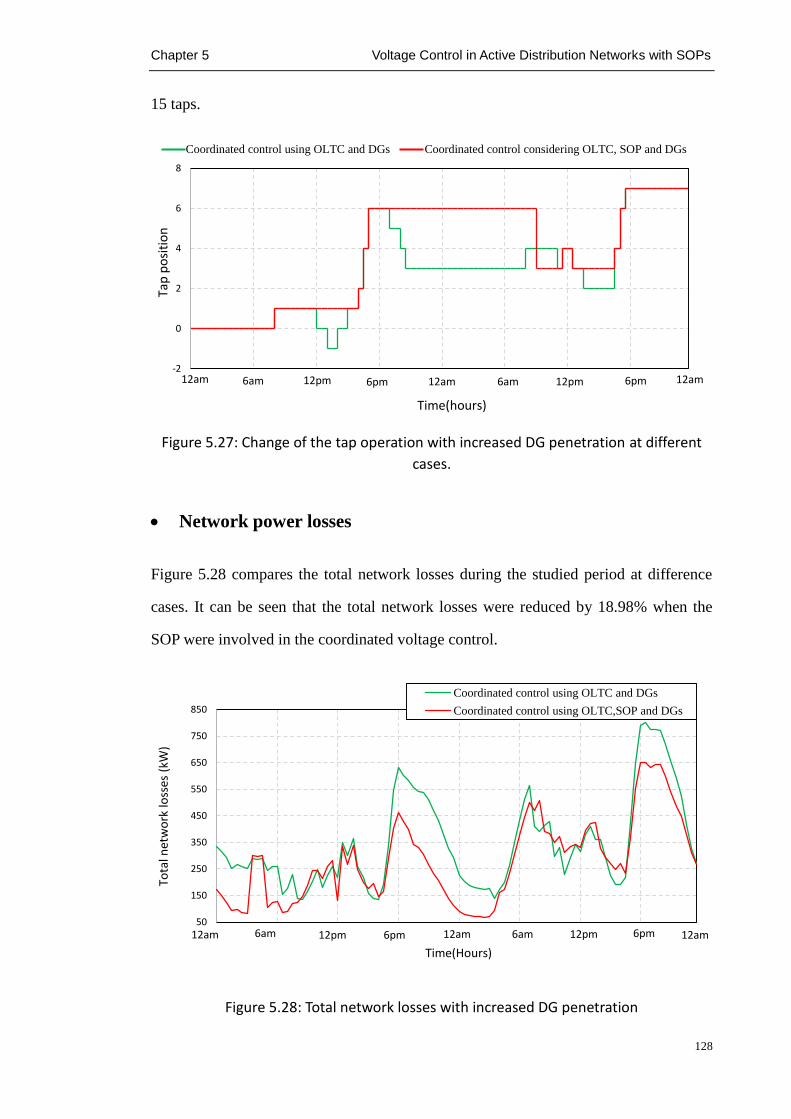
Chapter 5 Voltage Control in Active Distribution Networks with SOPs
128
15 taps.
Figure 5.27: Change of the tap operation with increased DG penetration at different
cases.
Network power losses
Figure 5.28 compares the total network losses during the studied period at difference
cases. It can be seen that the total network losses were reduced by 18.98% when the
SOP were involved in the coordinated voltage control.
Figure 5.28: Total network losses with increased DG penetration
-2
0
2
4
6
8Ta
p p
osi
tio
n
Time(hours)
Coordinated control using OLTC and DGs Coordinated control considering OLTC, SOP and DGs
12am 6am 6pm12pm 6pm 12am12pm12am 6am
50
150
250
350
450
550
650
750
850
Tota
l net
wo
rk lo
sses
(kW
)
Time(Hours)
Coordinated control using OLTC and DGs
Coordinated control using OLTC,SOP and DGs
12am 6am 6pm12pm 6pm 12am12pm12am 6am
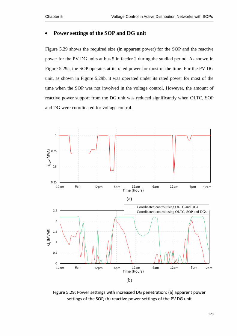
Chapter 5 Voltage Control in Active Distribution Networks with SOPs
129
Power settings of the SOP and DG unit
Figure 5.29 shows the required size (in apparent power) for the SOP and the reactive
power for the PV DG units at bus 5 in feeder 2 during the studied period. As shown in
Figure 5.29a, the SOP operates at its rated power for most of the time. For the PV DG
unit, as shown in Figure 5.29b, it was operated under its rated power for most of the
time when the SOP was not involved in the voltage control. However, the amount of
reactive power support from the DG unit was reduced significantly when OLTC, SOP
and DG were coordinated for voltage control.
(a)
(b)
Figure 5.29: Power settings with increased DG penetration: (a) apparent power
settings of the SOP, (b) reactive power settings of the PV DG unit
0.25
0.5
0.75
1
S SO
P (M
VA
)
Time (Hours)12am 6am 6pm12pm 6pm 12am12pm12am 6am
0
0.5
1
1.5
2
2.5
Qg
(MV
AR
)
Time (Hours)
Coordinated control using OLTC and DGs
Coordinated control using OLTC, SOP and DGs
12am 6am 6pm12pm 6pm 12am12pm12am 6am
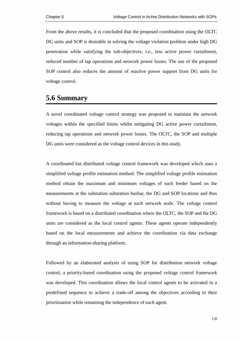
Chapter 5 Voltage Control in Active Distribution Networks with SOPs
130
From the above results, it is concluded that the proposed coordination using the OLTC
DG units and SOP is desirable in solving the voltage violation problem under high DG
penetration while satisfying the sub-objectives, i.e., less active power curtailment,
reduced number of tap operations and network power losses. The use of the proposed
SOP control also reduces the amount of reactive power support from DG units for
voltage control.
5.6 Summary
A novel coordinated voltage control strategy was proposed to maintain the network
voltages within the specified limits whilst mitigating DG active power curtailment,
reducing tap operations and network power losses. The OLTC, the SOP and multiple
DG units were considered as the voltage control devices in this study.
A coordinated but distributed voltage control framework was developed which uses a
simplified voltage profile estimation method. The simplified voltage profile estimation
method obtain the maximum and minimum voltages of each feeder based on the
measurements at the substation substation busbar, the DG and SOP locations and thus
without having to measure the voltage at each network node. The voltage control
framework is based on a distributed coordination where the OLTC, the SOP and the DG
units are considered as the local control agents. These agents operate independently
based on the local measurements and achieve the coordination via data exchange
through an information-sharing platform.
Followed by an elaborated analysis of using SOP for distribution network voltage
control, a priority-based coordination using the proposed voltage control framework
was developed. This coordination allows the local control agents to be activated in a
predefined sequence to achieve a trade-off among the objectives according to their
prioritisation while remaining the independence of each agent.

Chapter 5 Voltage Control in Active Distribution Networks with SOPs
131
Simulations verified the effectiveness of the proposed coordinated control strategy
under various load and generation conditions as well as high DG penetration. The
results showed that the proposed coordinated strategy has the capability to control
network voltage while also mitigating DG active power curtailment, reduce the tap
operations and avoid unnecessary increase in power losses in accordance with their
prioritisation. Simulation results also illuminated the role and importance of the SOP
for distribution network voltage control. It was found that the SOP is capable of
compensating the OLTC control, avoiding unnecessary DG curtailment, reducing the
number of tap operations and the network power losses as well as reducing the amount
of reactive power support from DG units for voltage control.

Chapter 6 Conclusions and Future Work
132
Conclusions and Future Work
HIS chapter outlines the major contributions and findings from the
research. It also presents further work around the research areas in this
thesis.
Chapter 6
T
Chapter 6 Conclusions and Future Work
133
6.1 Conclusions
Soft Open Points are power electronic devices installed in place of normally-open
points in electrical power distribution networks. They are able to provide active power
flow control, reactive power compensation and voltage regulation under normal
network operating conditions, as well as fast fault isolation and post-fault supply
restoration under abnormal conditions. The use of SOPs for the operation of MV
distribution networks was investigated from different perspectives including the control
of a back-to-back VSC based SOP, the benefits analysis of using SOPs and distribution
network voltage control with SOPs.
6.1.1 Control of a Back-to-Back VSC based SOP
Two control modes were developed for the operation of an SOP based on back-to-back
VSCs. The power flow control mode regulates both active and reactive power flows on
the connected feeders using a dual closed-loop current-controlled strategy. The supply
restoration mode provides fast post-fault supply restoration to the isolated loads using a
voltage and frequency control strategy. The operational principle and performance of
the back-to-back VSC based SOP with these two control modes were analysed under
both normal and abnormal network operating conditions:
Under normal conditions, the proposed SOP controller is able to provide both
instantaneous and longer duration power flow regulation between the connected
feeders as well as dynamic Volt/VAR control on both interface terminals.
During fault conditions, the SOP controller (power flow control mode) is able to
isolate both balanced and unbalanced network fault between the connected
feeders. Thus the fault propagation on the network can be limited and the
short-circuit current can be maintained as same as the radial network operation
without the SOP, which is important from a practical point of view as there is
little impact on the existing protection schemes.

Chapter 6 Conclusions and Future Work
134
Under post-fault supply restoration conditions, fast supply restoration (cold load
pickup) can be achieved through a smooth transition between the power flow
control mode and the supply restoration mode. For the transition from the power
flow control mode to the supply restoration mode, a soft cold load pickup process
was found preferred than a direct mode switching in order to avoid DC offset and
inrush issues of current which may trigger unexpected protection operations. For
the transition from the supply restoration mode to the power flow control mode,
the undesirable current impulse and voltage drop can be reduced after using the
voltage synchronization procedure and resetting the PI controllers.
6.1.2 Benefit Analysis of SOPs for MV Distribution Network
Operation
The operational benefits of using SOPs in MV distribution networks were investigated
focusing on power loss reduction, feeder load balancing and voltage profile
improvement. A steady state analysis framework was developed to quantify the benefits
of using SOPs. A generic power injection model of an SOP that is suitable for steady
state analysis was developed. Both physical limits and internal power losses of a typical
SOP device: back to back VSCs were considered in the model. The optimal SOP
operation was obtained using improved Powell’s Direction Set method. A combined
method considering both SOP and network reconfiguration were also proposed to
identify the benefits.
Based on the proposed framework, quantitative and sensitive analysis were conducted
and the key findings are listed as follows:
SOPs can contribute to significant power loss reduction, feeder load balancing
and voltage profile improvement. In the case study, using only one SOP achieved
similar improvement on network power loss reduction and feeder load balancing
compared to the case of using network reconfiguration with all branches

Chapter 6 Conclusions and Future Work
135
equipped with remotely controlled switches. By combining SOP and network
reconfiguration, the greatest improvements were obtained and smaller SOP sizes
were required.
When a large capacity of DGs were connected to the distribution network, SOPs
were found be able to significantly reduce the peak currents in feeders and
alleviate undesirable voltage excursions induced by the connection of DG and
demand. Therefore, SOPs can be used as an alternative to infrastructure upgrades
in accommodating distributed energy resources.
When the device efficiency (at rated power) decreased, the economic benefit of
SOP obtained from reducing total network power losses were lowered. However,
a greater positive impact were obtained when the system loading increased. The
requirements on SOP device efficiency for network loss reduction were reduced
when the system loading increased.
6.1.3 Voltage Control in Active Distribution Networks with SOPs
A novel coordinated voltage control strategy was proposed, in which OLTC, SOP and
DG units were considered as the controllable devices. The objective of the control
strategy was to maintain the network voltage within the specified limits whilst avoiding
unnecessary DG active power curtailment, reducing tap operations and network power
losses.
A coordinated but distributed voltage control framework was developed which uses a
simplified voltage profile estimation method. The simplified voltage profile estimation
method obtains the maximum and minimum voltages of each feeder based on the
measurements at the substation busbar, the DG and SOP locations and thus without
having to measure the voltage at each network node, which is able to reduce the
investment cost. The voltage control framework is based on a distributed control
scheme where the OLTC, the SOP and the DG units are considered as the local control
Chapter 6 Conclusions and Future Work
136
agents. These agents operate independently based on the local measurements and
achieve the coordination via data exchange through an information-sharing platform.
Followed by an analysis of using SOP for distribution network voltage control, a
priority-based coordination using the proposed control framework was developed. This
coordination, without affecting the independence of each agent, allows the local control
agents to be activated in a predefined sequence that can achieve a trade-off among the
objectives according to their prioritisation.
The results presented prove the capability of the proposed coordinated strategy to
achieve a trade-off among objectives in accordance with their prioritisation. Simulation
results also illuminated the role and importance of the SOP for distribution network
voltage control. It was found that the SOP is capable of compensating the OLTC
control, avoiding unnecessary DG active power curtailment, reducing the number of tap
operations and the network power losses as well as reducing the amount of reactive
power support from DG units for voltage control.
6.2 Future Work
The following future work was identified to extend the work reported in this thesis:
6.2.1 Use of other control strategies for the operation of the
back-to-back VSC based SOP
In this study, when a fault occurs on a feeder, a voltage and frequency control strategy
was used for the SOP to support isolated loads due to fault isolation. However, this
control strategy cannot limit the overcurrent on the interfacing VSC when a further
fault occurs on the isolated area. Hence additional protection of the interfacing VSC
needs to be considered. Therefore, control strategies that can provide the function of
limiting overcurrent should be investigated. One possible solution is to add an inner

Chapter 6 Conclusions and Future Work
137
current control loop to the current control strategy to limit the fault current.
A mode switching method were used to achieve a transition between the two control
modes of the SOP. The parameters of the PI controllers need to be determined carefully
upon the switching of the control modes in order to avoid unexpected transient
oscillations on the output voltage and current. Control strategies of the SOP that can
avoid the mode switching process should be investigated to improve the reliability.
6.2.2 Performances of the back-to-back VSC based SOP considering
different load types
The performances of a back-to-back VSC based SOP in MV distribution networks have
been investigated considering passive loads with constant impedances. However,
induction and/or synchronous machines (e.g., induction motor, synchronous generator)
are usually connected to distribution networks. These types of loads have different load
characteristics and, hence, may lead to different transient behaviours. Therefore, further
investigations on the performance of the proposed SOP device with different types of
network loads should be undertaken as future work.
6.2.3 Impacts of SOPs on feeder automation
Feeder automation is realized through automatic detection, isolation and
reconfiguration of faulted segments on distribution feeders. In this study, the capability
of the back-to-back VSC based SOP for fault isolation and post-fault supply restoration
was investigated. However, the interactions between the SOP and existing feeder
automation schemes were not considered.
For example, a simple form of feeder automation is achieved by deploying
combinations of reclosers and sectionalizers in a radial feeder. NOPs are used to allow
the radial feeders operating as an ‘open ring’. These devices (reclosers, sectionalizers
and NOPs) are coordinated to minimize the interruption of supply to customers under

Chapter 6 Conclusions and Future Work
138
fault conditions. When the NOPs are replaced with SOPs, the impact of the SOP on the
existing feeder automation scheme should be assessed. Additionally, the coordination
between the SOP and existing feeder automation scheme to avoid incoherent control
actions and approaches to obtain an optimal solution should be investigated.
6.2.4 Use of SOPs in unbalanced three-phase distribution networks
In this thesis, the use of SOPs in balanced three-phase distribution networks was
investigated. However, the domestic and some commercial customers connected to the
distribution network usually have single-phase connections. Therefore, the load in
distribution networks cannot be perfectly balanced. The imbalance in the three-phase
equipment needs to be reduced.
The SOP contains a common DC bus and hence enabling exchange of instantaneous
power between phases, which can be used to rebalance the power flows on the
connected feeders. Hence, new controllers should be investigated for the operation of
the SOP to address unbalanced three-phase conditions. In addition, the benefits of using
SOPs for the operation of unbalanced three-phase distribution networks should be
quantified and evaluated. Single phase power flow and optimization are suggested as
possible solution methods for the benefit analysis. New voltage control strategy to
address the voltage imbalance among the three phases should also be investigated.
6.2.5 Economic analysis of SOPs in MV distribution networks
This thesis investigated the technical benefits of SOPs in MV distribution networks.
However, a purely economic evaluation will give a better idea of weather the SOP
implementation is feasible, and where costs must be reduced to make it feasible. Hence,
further study on the economic analysis of SOPs should be undertake as future work.
The life cycle costs of SOPs should be quantified. The optimal amount, locations and
sizes of SOPs should also be determined considering the capital cost of SOPs. In

Chapter 6 Conclusions and Future Work
139
addition, the power loss reduction benefit of SOPs was performed in this thesis. In
order to further quantify the loss reduction benefit of SOPs, this study should be
extended to the study of quantifying energy power losses during a period.

Reference
140
Reference
[1] National Aeronautics and Space Administration, "The Current and Future
Consequences of Global Change", 08-Aug-2015. [Online]. Available:
http://climate.nasa.gov/effects/. [Accessed: 11-Sep-2015]
[2] T. Overbye et al., "The Electric Power Industry and Climate Change: Power Systems
Research Possibilities", Jun-2007. [Online]. Available:
http://pserc.wisc.edu/documents/publications/reports/2007_reports/pserc_climate_chan
ge_final_rpt_june07.pdf. [Accessed: 11-Sep-2015]
[3] European Commission, "EU action on climate", 15-July-2015. [Online]. Available:
http://ec.europa.eu/clima/policies/brief/eu/index_en.htm. [Accessed: 11-Sep-2015]
[4] Department of Energy and Climate Change, UK, "2010 to 2015 government policy:
greenhouse gas emissions", 08-May-2015. [Online]. Available:
https://www.gov.uk/government/publications/2010-to-2015-government-policy-greenh
ouse-gas-emissions/2010-to-2015-government-policy-greenhouse-gas-emissions.
[Accessed: 11-Sep-2015]
[5] Her Majesty's Goverment, UK, "The UK Renewable Energy Strategy", Jul-2009.
[Online]. Available:
http://www.biomassenergycentre.org.uk/pls/portal/docs/PAGE/RESOURCES/REF_LI
B_RES/PUBLICATIONS/THEUKRENEWABLEENERGYSTRATEGY2009.PDF.
[Accessed: 11-Sep-2015]
[6] K. Qian, "Modelling of electrical distribution systems with high penetration level of
distributed generation and electric vehicles," Ph.D thesis, Glasgow Caledonian
University, 2000.
[7] C. L. Masters et al., "Statistical evaluation of voltages in distribution systems with
embedded wind generation," IEE Proc. Gener. Transm. Distrib., vol. 147, no.4, pp.
207-212, Jul. 2000.
[8] I. P. D. Povh, D. Retzmann, and M. G. Weinhold, "Future Developments in Power
Industry," presented at the 4th IERE General Meeting and IERE Cental and Eastern
Europe Forum, Poland, 2014.
[9] International Energy Agency, "World Energy Outlook" 2009 [Online]. Available:
www.worldenergyoutlook.org/media/weowebsite/2009/WEO2009.pdf. [Accessed:
11-Sep-2015]
[10] Electricity North West, UK, "Capacity and carbon challenges", 2014. [Online].
Available:
http://www.enwl.co.uk/c2c/future-challenges/capacity-and-carbon-challenges
[11] Electricity North West, UK, "Impact of low carbon future", 2014. [Online]. Available:
http://www.enwl.co.uk/c2c/future-challenges/impact-of-a-low-carbon-future.
[Accessed: 11-Sep-2015]
[12] Ofgem, "Project Discovery Energy Market Scenarios", consultation document,
09-Oct-2009. [Online]. Available:

Reference
141
https://www.ofgem.gov.uk/ofgem-publications/40361/discoveryscenarioscondocfinal.p
df. [Accessed: 11-Sep-2015]
[13] H. Farhangi, "The path of the smart grid," Power and Energy Magazine, IEEE, vol. 8,
pp. 18-28, 2010.
[14] J. Zhu, Power System Operation Optimization, Second ed., Wiley-IEEE Press, 2008.
[15] U.S. Department of Energy, "Smart Grid System Report", Jul- 2009, [Online].
Available:
http://www.oe.energy.gov/sites/prod/files/oeprod/DocumentsandMedia/SGSRMain_09
0707_lowres.pdf. [Accessed: 11-Sep-2015]
[16] Department of Energy and Climate Change, UK, "Smart Grid Vision and Routemap
Smart", 27-Feb-2014. [Online]. Available:
https://www.gov.uk/.../Smart_Grid_Vision_and_RoutemapFINAL.pdf. [Accessed:
11-Sep-2015]
[17] Electricity Networks Strategy Group, UK, "'A Smart Grid Routemap’ Executive
Summary", Feb-2010. [Online]. Available:
http://webarchive.nationalarchives.gov.uk/20100919181607/http:/www.ensg.gov.uk/ass
ets/smartgrid_routemap_executive_summary_final.pdf. [Accessed: 11-Sep-2015]
[18] T. G. Richard Silversides, Tom Luth. "Power Electronics in Distribution System
Management", HubNet Position Paper, 05-Jan-2015. [Online]. Available:
www.hubnet.org.uk/filebyid/633/PE_Distribution.pdf. [Accessed: 11-Sep-2015]
[19] J. Ekanayake, N. Jenkins, K. Liyanage, J. Wu, and A. Yokoyama, Smart Grid:
Technology and Applications, Wiley Press, 2012.
[20] B. A. Robbins, C. N. Hadjicostis, and A. D. Dominguez-Garcia, "A Two-Stage
Distributed Architecture for Voltage Control in Power Distribution Systems," Power
Systems, IEEE Transactions on, vol. 28, pp. 1470-1482, 2013.
[21] European Network of Transmission System Operators, "Network Code on Operational
Security", 24-Sep-2013 [Online]. Available:
http://www.acer.europa.eu/Official_documents/Acts_of_the_Agency/Annexes%20to%
20ACER%20Recommendation%20092013%20on%20the%20NC%20on/The%20ame
nded%20Network%20Code%20on%20Operational%20Security%20resubmitted%20o
n%2024%20September.pdf. [Accessed: 11-Oct-2015].
[22] G. Strbac and J. Mutale, "Framework and Methodology for Pricing of Distribution
Networks with Distributed Generation - A report to OFGEM", Mar-2005 [Online].
Available:
https://www.ofgem.gov.uk/ofgem-publications/44458/10147-strbacmutale.pdf.
[Accessed: 11-Oct-2015].
[23] N. Hodge, "Power trip", 2010. [Online]. Available:
http://www.agcs.allianz.com/assets/PDFs/GRD/GRD%20individual%20articles/Power
_blackout_risks_article.pdf. [Accessed: 11-Oct-2015].
[24] T. Green et al., "Issues for Distribution System Operation at 2030", HubNet Position
Paper, 11-May-2014. [Online]. Available:
http://www.hubnet.org.uk/filebyid/523/2030GridOperation.pdf. [Accessed:
11-Oct-2015].

Reference
142
[25] OFGEM, UK, "Losses Incentive Mechanism", 2015. [Online]. Available:
https://www.ofgem.gov.uk/electricity/distribution-networks/losses-incentive-mechanis
m. [Accessed: 11-Oct-2015].
[26] OFGEM, UK, "Decision on restatement of 2009-10 data and closing out the DPCR4
losses incentive mechanism", 21-Mar-2014. [Online]. Available:
https://www.ofgem.gov.uk/ofgem-publications/86757/decisiononclosingoutdprc4losses
mechanism-mar-14.pdf. [Accessed: 11-Oct-2015].
[27] S. Civanlar, J. J. Grainger, H. Yin, and S. S. H. Lee, "Distribution feeder
reconfiguration for loss reduction," Power Delivery, IEEE Transactions on, vol. 3, pp.
1217-1223, 1988.
[28] I. Roytelman and V. Ganesan, "Coordinated local and centralized control in distribution
management systems," Power Delivery, IEEE Transactions on, vol. 15, pp. 718-724,
2000.
[29] R. S. Rao, K. Ravindra, K. Satish, and S. V. L. Narasimham, "Power Loss
Minimization in Distribution System Using Network Reconfiguration in the Presence
of Distributed Generation," Power Systems, IEEE Transactions on, vol. 28, pp.
317-325, 2013.
[30] A. Merlin and H. Back, "Search for a minimal-loss operating spanning tree
configuration in an urban power distribution system," presented at the Proc. 5th Power
System Computation Conforence, Cambridge, 1975.
[31] K. Nara, A. Shiose, M. Kitagawa, and T. Ishihara, "Implementation of genetic
algorithm for distribution systems loss minimum re-configuration," Power Systems,
IEEE Transactions on, vol. 7, pp. 1044-1051, 1992.
[32] D. Das, "A fuzzy multiobjective approach for network reconfiguration of distribution
systems," Power Delivery, IEEE Transactions on, vol. 21, pp. 202-209, 2006.
[33] J. Young-Jae, K. Jae-Chul, O. K. Jin, S. Joong-Rin, and K. Y. Lee, "An efficient
simulated annealing algorithm for network reconfiguration in large-scale distribution
systems," Power Delivery, IEEE Transactions on, vol. 17, pp. 1070-1078, 2002.
[34] Y. Yu and J. Wu, "Loads combination method based core schema genetic shortest-path
algorithm for distribution network reconfiguration," in Proceedings of Power System
Technology Conference, 2002, pp. 1729-1733, vol 3.
[35] A. Ahuja, S. Das, and A. Pahwa, "An AIS-ACO Hybrid Approach for Multi-Objective
Distribution System Reconfiguration," Power Systems, IEEE Transactions on, vol. 22,
pp. 1101-1111, 2007.
[36] C. Chao-Shun, T. Cheng-Ta, L. Chia-Hung, H. Wei-Lin, and K. Te-Tien, "Loading
Balance of Distribution Feeders With Loop Power Controllers Considering
Photovoltaic Generation," Power Systems, IEEE Transactions on, vol. 26, pp.
1762-1768, 2011.
[37] W. Cao, J. Wu, and N. Jenkins. "Feeder Load Balancing in MV Distribution Networks
Using Soft Normally-Open Points,"in IEEE Innovative Smart Grid Technologies
Conference Europe, 2014, PP 1-6.
[38] S. K. Bhattacharya and S. K. Goswami, "Distribution Network Reconfiguration
Considering Protection Coordination Constraints," Electric Power Components and

Reference
143
Systems, vol. 36, pp. 1150-1165, 2008.
[39] S. Rahimi, M. Marinelli, and F. Silvestro, "Evaluation of requirements for Volt/Var
control and optimization function in distribution management systems," in IEEE
International Energy Conference and Exhibition (ENERGYCON), 2012, pp. 331-336.
[40] F. A. Viawan and D. Karlsson, "Voltage and Reactive Power Control in Systems With
Synchronous Machine-Based Distributed Generation," Power Delivery, IEEE
Transactions on, vol. 23, pp. 1079-1087, 2008.
[41] H. E. Z. Farag, E. F. El-Saadany, and R. Seethapathy, "A Two Ways
Communication-Based Distributed Control for Voltage Regulation in Smart
Distribution Feeders," Smart Grid, IEEE Transactions on, vol. 3, pp. 271-281, 2012.
[42] L. Xiaohu, A. Aichhorn, L. Liming, and L. Hui, "Coordinated Control of Distributed
Energy Storage System With Tap Changer Transformers for Voltage Rise Mitigation
Under High Photovoltaic Penetration," Smart Grid, IEEE Transactions on, vol. 3, pp.
897-906, 2012.
[43] M. J. E. Alam, K. M. Muttaqi, and D. Sutanto, "A Multi-Mode Control Strategy for
VAr Support by Solar PV Inverters in Distribution Networks," Power Systems, IEEE
Transactions on, vol. 30, pp. 1316-1326, 2015.
[44] C. Joon-Ho and K. Jae-Chul, "Advanced voltage regulation method of power
distribution systems interconnected with dispersed storage and generation systems,"
Power Delivery, IEEE Transactions on, vol. 16, pp. 329-334, 2001.
[45] F. Shahnia, M. T. Wishart, and A. Ghosh, "Voltage regulation, power balancing and
battery storage discharge control by smart demand side management and
multi-objective decision making," in Power Engineering Conference (AUPEC), 2013
Australasian Universities, 2013, pp. 1-5.
[46] N. Yorino, Y. Zoka, M. Watanabe, and T. Kurushima, "An Optimal Autonomous
Decentralized Control Method for Voltage Control Devices by Using a Multi-Agent
System," Power Systems, IEEE Transactions on, vol. 30, pp. 2225-2233, 2015.
[47] P. M. S. Carvalho, P. F. Correia, and L. A. F. Ferreira, "Distributed Reactive Power
Generation Control for Voltage Rise Mitigation in Distribution Networks," Power
Systems, IEEE Transactions on, vol. 23, pp. 766-772, 2008.
[48] A. Kulmala, S. Repo, Ja, x, and P. rventausta, "Coordinated Voltage Control in
Distribution Networks Including Several Distributed Energy Resources," Smart Grid,
IEEE Transactions on, vol. 5, pp. 2010-2020, 2014.
[49] P. N. Vovos, A. E. Kiprakis, A. R. Wallace, and G. P. Harrison, "Centralized and
Distributed Voltage Control: Impact on Distributed Generation Penetration," Power
Systems, IEEE Transactions on, vol. 22, pp. 476-483, 2007.
[50] M. R. Kleinberg, K. Miu, N. Segal, H. Lehmann, and T. R. Figura, "A Partitioning
Method for Distributed Capacitor Control of Electric Power Distribution Systems,"
Power Systems, IEEE Transactions on, vol. 29, pp. 637-644, 2014.
[51] M. B. Liu, C. A. Canizares, and W. Huang, "Reactive Power and Voltage Control in
Distribution Systems With Limited Switching Operations," Power Systems, IEEE
Transactions on, vol. 24, pp. 889-899, 2009.
[52] M. A. Azzouz, M. F. Shaaban, and E. F. El-Saadany, "Real-Time Optimal Voltage

Reference
144
Regulation for Distribution Networks Incorporating High Penetration of PEVs," Power
Systems, IEEE Transactions on, vol. 30, pp. 3234-3245, 2015.
[53] T. Senjyu, Y. Miyazato, A. Yona, N. Urasaki, and T. Funabashi, "Optimal Distribution
Voltage Control and Coordination With Distributed Generation," Power Delivery, IEEE
Transactions on, vol. 23, pp. 1236-1242, 2008.
[54] K. Young-Jin, A. Seon-Ju, H. Pyeong-Ik, P. Gi-Chan, and M. Seung-Il, "Coordinated
Control of a DG and Voltage Control Devices Using a Dynamic Programming
Algorithm," Power Systems, IEEE Transactions on, vol. 28, pp. 42-51, 2013.
[55] H. E. Z. Farag and E. F. El-Saadany, "A Novel Cooperative Protocol for Distributed
Voltage Control in Active Distribution Systems," Power Systems, IEEE Transactions
on, vol. 28, pp. 1645-1656, 2013.
[56] M. E. Baran and I. M. El-Markabi, "A Multiagent-Based Dispatching Scheme for
Distributed Generators for Voltage Support on Distribution Feeders," Power Systems,
IEEE Transactions on, vol. 22, pp. 52-59, 2007.
[57] M. E. Elkhatib, R. El-Shatshat, and M. M. A. Salama, "Novel Coordinated Voltage
Control for Smart Distribution Networks With DG," Smart Grid, IEEE Transactions on,
vol. 2, pp. 598-605, 2011.
[58] D. Divan, R. Moghe, and A. Prasai, "Power Electronics at the Grid Edge : The key to
unlocking value from the smart grid," Power Electronics Magazine, IEEE, vol. 1, pp.
16-22, 2014.
[59] Scottish and Southern Energy, "technical Appendix 12 - Making Innovation Happen ",
2013. [Online]. Available:
http://www.energyinnovationcentre.com/wp-content/uploads/SSEPD-Innovation-Strate
gy.pdf. [Accessed: 11-Oct-2015].
[60] C. Goodhand. "Ofgem - LCNF Tier 1 project: 33kV Superconducting Fault Current
Limiter", 2015. [Online]. Available:
https://www.ofgem.gov.uk/ofgem-publications/94151/33kvsfclfinalclosedownreportver
10final-pdf. [Accessed: 11-Oct-2015].
[61] UK Power Networks, " Ofgem - LCNF Tier 2 project: Flexible Urban Networks Low
Voltage", 2014 [Online]. Available:
http://innovation.ukpowernetworks.co.uk/innovation/en/Projects/tier-2-projects/Flexibl
e-Urban-Networks-Low-Voltage/Project-Documents/Overview+Flexible+Urban+Netw
orks+Low+Voltage-+Jan+2014.pdf. [Accessed: 11-Oct-2015].
[62] M. McGranaghan, "Intelligent Universal Transformer Design and Applications",
Jun-2009. [Online]. Available:
http://www.cired.net/publications/cired2009/main_sessions/Session%201/Main%20Ses
sion%201%20pdfs/Block%201/S1%201032.pdf. [Accessed: 11-Oct-2015].
[63] D. J. Rogers and T. C. Green, "An Active-Shunt Diverter for On-load Tap Changers,"
Power Delivery, IEEE Transactions on, vol. 28, pp. 649-657, 2013.
[64] G. L. A. Ghosh, Power Quality Enhancement Using Custom Power Devices: Springer,
2002.
[65] Y. Pal, A. Swarup, and B. Singh, "A Review of Compensating Type Custom Power
Devices for Power Quality Improvement," in Power System Technology and IEEE

Reference
145
Power India Conference, 2008, pp. 1-8.
[66] Scottish and Southern Energy, "OFGEM - LCNF Tier 1 Close-Down Report",
28-Feb-2013. [Online]. Available:
https://www.ofgem.gov.uk/ofgem-publications/45826/sset1002-lv-monitoring-lcnf-t1-c
lose-down-report-130228.pdf. [Accessed: 11-Oct-2015].
[67] J. M. Bloemink and T. C. Green, "Increasing distributed generation penetration using
soft normally-open points," in IEEE Power and Energy Society General Meeting, 2010,
pp. 1-8.
[68] J. M. Bloemink and T. C. Green, "Increasing photovoltaic penetration with local energy
storage and soft normally-open points," in IEEE Power and Energy Society General
Meeting, 2011, pp. 1-8.
[69] E. Romero-Ramos, et al., "Assessing the loadability of active distribution networks in
the presence of DC controllable links," Generation, Transmission & Distribution, IET,
vol. 5, pp. 1105-1113, 2011.
[70] J. M. Bloemink and T. C. Green, "Benefits of Distribution-Level Power Electronics for
Supporting Distributed Generation Growth," Power Delivery, IEEE Transactions on,
vol. 28, pp. 911-919, 2013.
[71] N. Okada, M. Takasaki, H. Sakai, and S. Katoh, "Development of a 6.6 kV - 1 MVA
Transformerless Loop Balance Controller," in IEEE Power Electronics Specialists
Conference, 2007, pp. 1087-1091.
[72] M. Noroozian, L. Angquist, M. Ghandhari, and G. Andersson, "Use of UPFC for
optimal power flow control," Power Delivery, IEEE Transactions on, vol. 12, pp.
1629-1634, 1997.
[73] M. Takeshita and H. Sugihara, "Effect of fault current limiting of UPFC for power flow
control in loop transmission," in IEEE Transmission and Distribution Conference and
Exhibition 2002: Asia Pacific., 2002, pp. 2032-2036.
[74] M. Barragan, et al., "Operational benefits of multiterminal DC-links in active
distribution networks," in IEEE Power and Energy Society General Meeting, 2012, pp.
1-6.
[75] G. Fang and M. R. Iravani, "A Control Strategy for a Distributed Generation Unit in
Grid-Connected and Autonomous Modes of Operation," Power Delivery, IEEE
Transactions on, vol. 23, pp. 850-859, 2008.
[76] N. Okada, "Verification of Control Method for a Loop Distribution System using Loop
Power Flow Controller," in IEEE Power Systems Conference and Exposition, 2006, pp.
2116-2123.
[77] A. Marano-Marcolini, E. Romero-Ramos, A. Gomez-Exposito, J. M. Maza-Ortega, and
J. L. Martinez-Ramos, "Enhancing the integration of renewable sources in distribution
systems using DC-links," in IEEE Sustainable Alternative Energy (SAE) Conference,
2009, pp. 1-5.
[78] M. A. Sayed and T. Takeshita, "All Nodes Voltage Regulation and Line Loss
Minimization in Loop Distribution Systems Using UPFC," Power Electronics, IEEE
Transactions on, vol. 26, pp. 1694-1703, 2011.
[79] J. M. Maza-Ortega, et al., "Voltage source converter-based topologies to further

Reference
146
integrate renewable energy sources in distribution systems," Renewable Power
Generation, IET, vol. 6, pp. 435-445, 2012.
[80] R. A. A. de Graaff, J. M. Myrzik, W. L. Kling, and J. H. R. Enslin, "Series Controllers
in Distribution Systems - Facilitating Increased Loading and Higher DG Penetration,"
in IEEE Power Systems Conference and Exposition, 2006, pp. 1926-1930.
[81] R. A. A. de Graaff, J. M. A. Myrzik, W. L. Kling, and J. H. R. Enslin, "Intelligent
Nodes in Distribution Systems - Optimizing Steady State Settings," in Power Tech,
2007 IEEE Lausanne, 2007, pp. 391-395.
[82] N. Flourentzou, V. G. Agelidis, and G. D. Demetriades, "VSC-Based HVDC Power
Transmission Systems: An Overview," Power Electronics, IEEE Transactions on, vol.
24, pp. 592-602, 2009.
[83] S. G. Johansson., G. A. Splund., R. Jansson., and E. A. Rudervall., "Power system
stability benefits with VSC dc-transmission systems," in CIGRE Paris, 2004, pp. 1-8.
[84] B. Jacobson, Y. Jiang-Hafner, G. A. P. Rey, M. Jeroense, A. Gustafsson, and M.
Bergkvist, "HVDC with Voltage Source Converters and Extruded cables for up to +/-
300 kV and 1000 MW," in CIGRE Sessions, Paris, 2006, pp. 1-8.
[85] N. R. Chaudhuri, R. Majumder, B. Chaudhuri, and P. Jiuping, "Stability Analysis of
VSC MTDC Grids Connected to Multimachine AC Systems," Power Delivery, IEEE
Transactions on, vol. 26, pp. 2774-2784, 2011.
[86] J. M. Espi Huerta, J. Castello-Moreno, J. R. Fischer, and R. Garcia-Gil, "A
Synchronous Reference Frame Robust Predictive Current Control for Three-Phase
Grid-Connected Inverters," Industrial Electronics, IEEE Transactions on, vol. 57, pp.
954-962, 2010.
[87] I. J. Balaguer, L. Qin, Y. Shuitao, U. Supatti, and P. Fang Zheng, "Control for
Grid-Connected and Intentional Islanding Operations of Distributed Power
Generation," Industrial Electronics, IEEE Transactions on, vol. 58, pp. 147-157, 2011.
[88] L. G. B. Rolim, D. R. da Costa, and M. Aredes, "Analysis and Software
Implementation of a Robust Synchronizing PLL Circuit Based on the pq Theory,"
Industrial Electronics, IEEE Transactions on, vol. 53, pp. 1919-1926, 2006.
[89] S. Cole, J. Beerten, and R. Belmans, "Generalized Dynamic VSC MTDC Model for
Power System Stability Studies," Power Systems, IEEE Transactions on, vol. 25, pp.
1655-1662, 2010.
[90] B. Silva, C. L. Moreira, H. Leite, and J. A. Lopes, "Control Strategies for AC Fault
Ride Through in Multiterminal HVDC Grids," Power Delivery, IEEE Transactions on,
vol. 29, pp. 395-405, 2014.
[91] H. Nikkhajoei and R. H. Lasseter, "Microgrid Protection," in IEEE Power Engineering
Society General Meeting, 2007, pp. 1-6.
[92] N. T. Stringer, "The effect of DC offset on current-operated relays," Industry
Applications, IEEE Transactions on, vol. 34, pp. 30-34, 1998.
[93] M. E. Baran and F. F. Wu, "Optimal sizing of capacitors placed on a radial distribution
system," Power Delivery, IEEE Transactions on, vol. 4, pp. 735-743, 1989.
[94] G. Daelemans, K. Srivastava, M. Reza, S. Cole, and R. Belmans, "Minimization of
steady-state losses in meshed networks using VSC HVDC," in IEEE Power & Energy

Reference
147
Society General Meeting, 2009, pp. 1-5.
[95] M. J. D. Powell, "An efficient method for finding the minimum of a function of several
variables without calculating derivatives," The Computer Journal, vol. 7, pp. 155-162,
1964.
[96] L. Cheng-Ling, C. Tai-Ning, L. Yuan-Yao, H. Pin, and R.-K. Lee, "Powell's method for
designing optical multilayer thin-film filters," in 15th OptoeElectronics and
Communications Conference, 2010, pp. 388-389.
[97] S. Lazarou, V. Vita, and L. Ekonomou, "Application of powell's optimisation method
for the optimal number of wind turbines in a wind farm," Science, Measurement &
Technology, IET, vol. 5, pp. 77-80, 2011.
[98] H. Cho, A. D. Smith, and P. Mago, "Combined cooling, heating and power: A review of
performance improvement and optimization," Applied Energy, vol. 136, pp. 168-185,
2014.
[99] M. E. Baran and F. F. Wu, "Network reconfiguration in distribution systems for loss
reduction and load balancing," Power Delivery, IEEE Transactions on, vol. 4, pp.
1401-1407, 1989.
[100] UK Statutory Instruments, No. 2665, “The Electricity Safety, Quality and Continuity
Regulations,” 2002.
[101] M. A. Azzouz, M. F. Shaaban, and E. F. El-Saadany, "Real-Time Optimal Voltage
Regulation for Distribution Networks Incorporating High Penetration of PEVs," Power
Systems, IEEE Transactions on, vol. PP, pp. 1-12, 2015.
[102] A. E. Kiprakis and A. R. Wallace, "Maximising energy capture from distributed
generators in weak networks," Generation, Transmission and Distribution, IEE
Proceedings-, vol. 151, pp. 611-618, 2004.
[103] "IEEE Application Guide for IEEE Std 1547(TM), IEEE Standard for Interconnecting
Distributed Resources with Electric Power Systems," IEEE Std 1547.2-2008, pp.
1-217,

Publications
148
Publications
Journal Paper:
[1] W. Cao, J. Wu, C. Wang, T. Green and N. Jenkins, “Operating Principle of Soft
Open Points for Electrical Distribution Network Operation” Applied Energy, Vol.
164, pp 245-247, Feb. 2016. 10.1016/j.apenergy.2015.12.005
[2] W. Cao, J. Wu, C. Wang, T. Green and N. Jenkins, “Benefits Analysis of Soft Open
Points for Electrical Distribution Network Operation” Applied Energy, Vol. 165, pp
36-47, Mar. 2016. 10.1016/j.apenergy.2015.12.022
Conference Paper:
[1] W. Cao, J. Wu, and N. Jenkins, “Feeder Load Balancing in MV Distribution
Networks Using Soft Normally-Open Points," in IEEE PES Innovative Smart Grid
Technologies (ISGT), Europe, 2014, PP 1-6.
[2] W. Cao, J. Wu, and Z. Huang, “Soft Open Points for Supply Restoration in
Medium Voltage Distribution Networks” accepted for publication in IEEE PES
Asia-Pacific Power and Energy Engineering Conference (APPEEC), Australia,
2015.
[3] A. Aithal, C. Long, W. Cao, J. Wu, “Impact of Soft Open Point on Feeder
Automation” accepted for publication in IEEE ENERGYCON, Europe, 2016.

Appendix A
149
Appendix A: Data for the Two-Feeder Test
Network
Table A.2 Network Parameters for the SOP study in Chapter 5
Feeder
No.
From
bus
To
bus
Line Impedance parameters Length
(km)
load parameters at
receiving buses
r (ohm/km) x (ohm/km) P (kW) Q (kVar)
2 0 1 0.203 0.1034 1 60 25
2 1 2 0.2842 0.1447 1 60 25
2 2 3 1.059 0.9337 1 60 20
2 3 4 0.8042 0.7006 1 120 70
2 4 5 0.5075 0.2585 1 200 600
2 5 6 0.9744 0.963 1 150 70
2 6 7 0.3105 0.3619 1 210 100
2 7 8 0.341 0.5302 1 60 40
1 0 1 0.0922 0.047 1 100 60
1 1 2 0.493 0.2511 1 90 40
1 2 3 0.366 0.1864 1 120 80
1 3 4 0.3811 0.1941 1 60 30
1 4 5 0.819 0.707 1 60 20
1 5 6 0.1872 0.6188 1 200 100
1 6 7 0.7114 0.2351 1 200 100
1 7 8 1.03 0.74 1 60 20
1 8 9 1.044 0.74 1 60 20
1 9 10 0.1966 0.065 1 45 30
1 10 11 0.3744 0.1238 1 60 35
1 11 12 1.468 1.155 1 60 35
1 12 13 0.5416 0.7129 1 120 80

Appendix A
150
1 13 14 0.591 0.526 1 60 10
1 14 15 0.7463 0.545 1 60 20
1 15 16 1.289 1.721 1 60 20
1 16 17 0.732 0.574 1 90 40

Appendix B
151
Appendix B: Data for the Four-Feeder Test
Network
Table B.3 Network Parameters for the Case study in Chapter 5
Feeder
No.
From
bus
To
bus
Line Impedance parameters Length
(km)
Rated loading at
receiving buses
r (ohm/km) x (ohm/km) P (kw) Q (kvar)
1 0 1 0.55 0.4 1 228 171
1 1 2 0.55 0.4 1 273.6 79.8
1 2 3 0.55 0.4 1 112.5 124.26
1 3 4 0.55 0.4 1 171 228
1 4 5 0.55 0.4 1 79.8 273.6
1 5 6 0.55 0.4 1 256.5 124.26
1 6 7 0.55 0.4 1 228 171
1 7 8 0.55 0.4 1 163.2 68.6
2 0 1 0.55 0.4 1 196 147
2 1 2 0.55 0.4 1 235.2 68.6
2 2 3 0.55 0.4 1 220.5 106.82
2 3 4 0.55 0.4 1 147 196
2 4 5 0.55 0.4 1 68.6 235.2
2 5 6 0.55 0.4 1 235.2 68.6
2 6 7 0.55 0.4 1 196 147
2 7 8 0.55 0.4 1 235.2 68.6
2 8 9 0.55 0.4 1 196 147
2 9 10 0.55 0.4 1 343.2 100.1
3 0 1 0.55 0.4 1 286 214.5
3 1 2 0.55 0.4 1 321.75 155.87
3 2 3 0.55 0.4 1 307.2 100.1
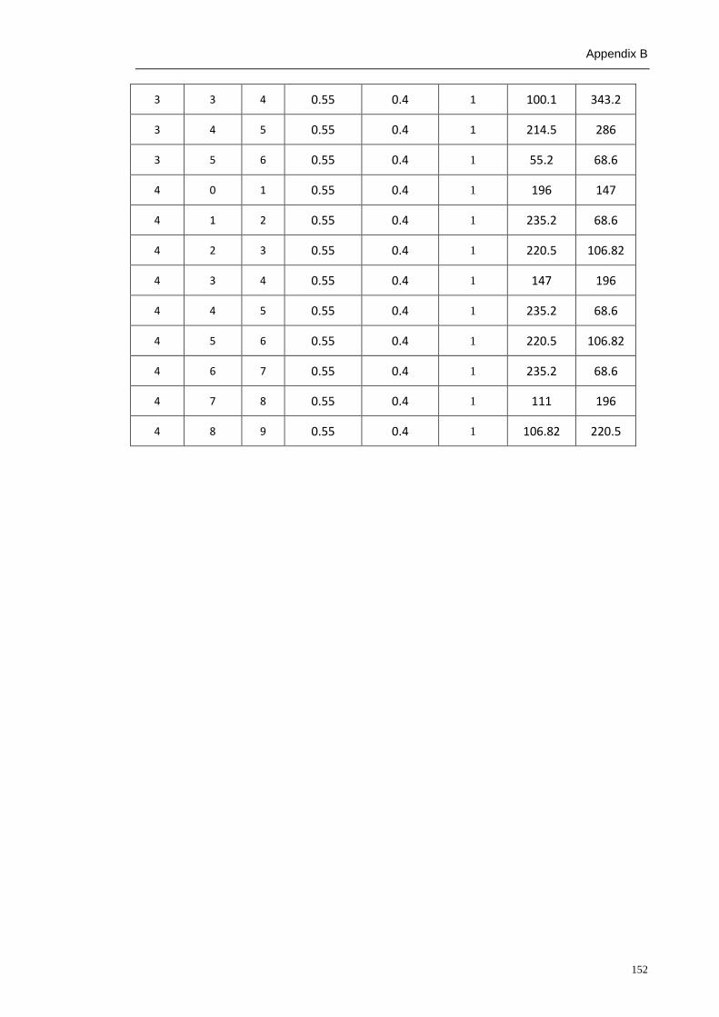
Appendix B
152
3 3 4 0.55 0.4 1 100.1 343.2
3 4 5 0.55 0.4 1 214.5 286
3 5 6 0.55 0.4 1 55.2 68.6
4 0 1 0.55 0.4 1 196 147
4 1 2 0.55 0.4 1 235.2 68.6
4 2 3 0.55 0.4 1 220.5 106.82
4 3 4 0.55 0.4 1 147 196
4 4 5 0.55 0.4 1 235.2 68.6
4 5 6 0.55 0.4 1 220.5 106.82
4 6 7 0.55 0.4 1 235.2 68.6
4 7 8 0.55 0.4 1 111 196
4 8 9 0.55 0.4 1 106.82 220.5