Soft Matter

PAPER

Dow

nloa

ded

by E

mor

y U

nive

rsity

on

27 F

ebru

ary

2013

Publ

ishe

d on

13

Febr

uary

201

3 on

http

://pu

bs.r

sc.o

rg |

doi:1

0.10

39/C

3SM

2728

7G

View Article OnlineView Journal | View Issue

Department of Physics, Emory University, At

emory.edu

† Current address: Department of MeCalifornia, Santa Barbara, CA 93106, USA

‡ Current address: Soochow University, Su

Cite this: Soft Matter, 2013, 9, 3424

Received 4th October 2012Accepted 29th January 2013

DOI: 10.1039/c3sm27287g

www.rsc.org/softmatter

3424 | Soft Matter, 2013, 9, 3424–34

Experimental study of forces between quasi-two-dimensional emulsion droplets near jamming

Kenneth W. Desmond,† Pearl J. Young, Dandan Chen‡ and Eric R. Weeks*

We experimentally study the jamming of quasi-two-dimensional emulsions. Our experiments consist of oil-

in-water emulsion droplets confined between two parallel plates. From the droplet outlines, we can

determine the forces between every droplet over a wide range of area fractions f. We study three

bidisperse samples that jam at area fractions fc z 0.86. Our data show that for f > fc, the contact

numbers and pressure have power-law dependence on f � fc in agreement with the critical scaling

found in numerical simulations. Furthermore, we see a link between the interparticle force law and the

exponent for the pressure scaling, supporting prior computational observations. We also observe linear-

like force chains (chains of large inter-droplet forces) that extend over 10 particle lengths, and examine

the origin of their linearity. We find that the relative orientation of large force segments are random

and that the tendency for force chains to be linear is not due to correlations in the direction of

neighboring large forces, but instead occurs because the directions are biased towards being linear to

balance the forces on each droplet.

1 Introduction

A liquid to amorphous-solid transition, also known as ajamming transition, occurs in a wide variety of so materialssuch as colloids, emulsions, foams, and sand. In general thejamming transition is due to an increase in the particleconcentration f; the particles become sufficiently crowded sothat microscopic rearrangements are unable to occur whenexternal stresses are applied.1–3 At a critical fc the system jamsinto a rigid structure, and many of the material properties areknown2,4 to scale with a power-law dependence on (f � fc).While these somaterials have obvious differences, it has beenpostulated that there are universal features of the jammingtransition that all these materials share in common such ascritical scaling and the emergence of force chains.

In all systems above the jamming point, particles press intoone another and deform. As the density increases, new contactsform and particles deform more, increasing the pressure.Interesting, both the average number of contacts z and thepressure P show critical-like scaling relative to the jammingpoint. In experiments and simulations, both 2D and 3D, theaverage number of contacts scales as z � zc ¼ A(f � fc)

bz, wherezc and A depend on the dimension and bz ¼ 1/2 regardless ofdimension.5–11 Similarly, experiments and simulations also

lanta, GA 30322, USA. E-mail: erweeks@

chanical Engineering, University of.

zhou, Jiangsu, China.

36

found power law scaling of P with exponent bP.5–8,10,12,13 Thesimulations revealed that the value of bP depends on the detailson the interparticle force law.5–8 If this pressure scaling andconnection between bP and the interparticle force law extends toexperiments, then this would demonstrate a direct link betweenthe interaction of the constituent particles and the bulk prop-erties of the sample, as the bulk modulus can be found fromP (f).

Another observed feature of jammed systems is the spatialheterogeneity of the particle–particle contact forces. In experi-ments and simulations, both 2D and 3D, the shape of theprobability distribution of forces is broad with an exponentiallike tail.7,8,10,11,14–23 The largest forces tend to form chain struc-tures that bear the majority of the load.14–20 These force chainsare responsible for providing rigidity of jammed materials toexternal stresses and are related to many other bulk proper-ties.14,15,24,25 In prior experiments on 3D emulsions, the structureof the force chains was studied directly, where force chainsextended over 10 particle diameters with a persistence length of3–4 particle diameters.17,21,22

There have been theoretical attempts to understand forcechains and the probability distribution of forces, such as theq-model of Coppersmith et al.,26 directed-force chain networksof Socolar's group,27 and simulations.28–30 While some of thesemodels successfully predict certain properties of the forcenetwork, they cannot explain the physical origins of forcechains, and therefore, others took an ensemble approach todescribe the physical orgins, with different choices for ensem-bles.22,31–37 The two basic assumptions of these ensemblemodels are that the forces on a droplet must balance and the

This journal is ª The Royal Society of Chemistry 2013

Paper Soft Matter

Dow

nloa

ded

by E

mor

y U

nive

rsity

on

27 F

ebru

ary

2013

Publ

ishe

d on

13

Febr

uary

201

3 on

http

://pu

bs.r

sc.o

rg |

doi:1

0.10

39/C

3SM

2728

7GView Article Online

forces between neighboring droplets are uncorrelated. Toexplain the structure of the force chains observed in 3D emul-sion studies, Brujic et al.21,22 and Zhou et al.17,34 proposed anensemble model at the single particle scale that provides anaccurate physical description for the origin of force chains. Thismodel has not been applied to 2D systems.

In this paper, we introduce a new experimental system tostudy the universal nature of the jamming transition. Oursystem consist of quasi-2D so deformable droplets with nostatic friction forces. In the Appendix, we describe our methodto determine the forces between droplets in contact to within16%, signicantly better than prior studies of foams11 andcomparable to photoelastic disks.16 Using our experimentalmodel system, we nd power-law scaling for the coordinationnumber and pressure (Section 4.2), we observe a relationshipbetween the interparticle force law and bP (Section 4.2), and seea distribution of contact forces similar to prior work (Section4.3). Further, we conrm the assumptions of the Brujic–Zhoumodel apply to our data and that the model well-describes our2D data (Section 4.4). This work provides an in depth studycomparing data from our experimental model system to othernumerical simulations, theory, and experimental systems, thusfurthering our understanding of the jamming transition andsupporting the applicability of ideas of jamming to a newsystem.

2 Experimental method

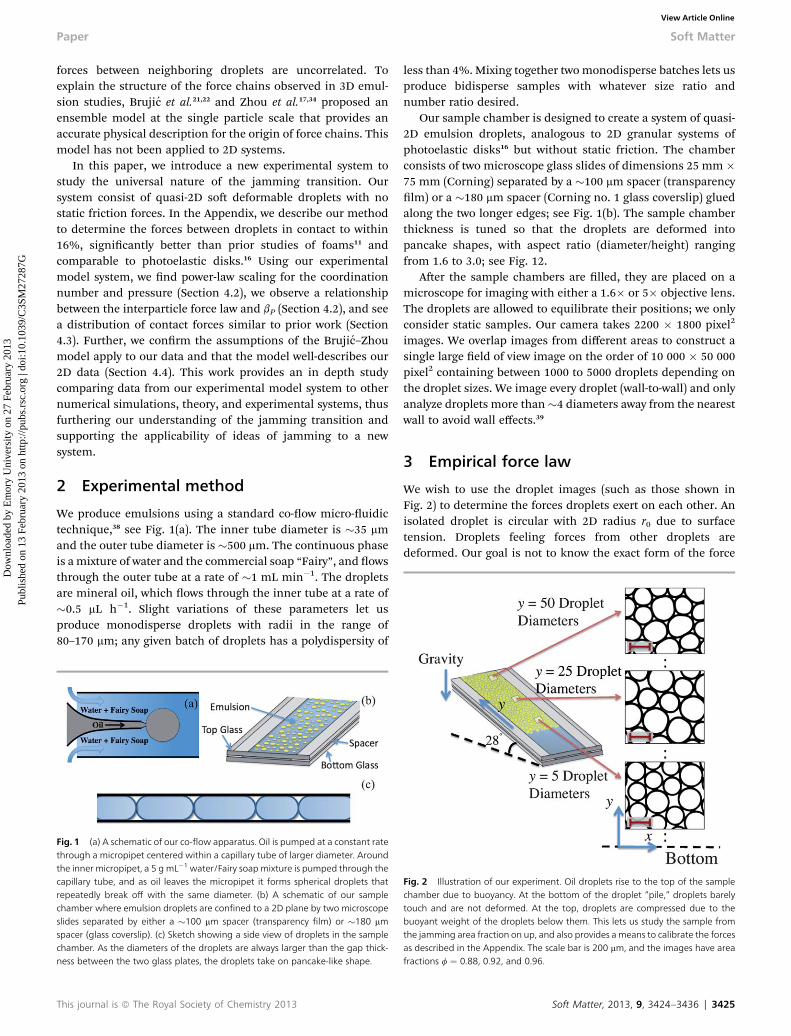
We produce emulsions using a standard co-ow micro-uidictechnique,38 see Fig. 1(a). The inner tube diameter is �35 mmand the outer tube diameter is �500 mm. The continuous phaseis amixture of water and the commercial soap “Fairy”, and owsthrough the outer tube at a rate of �1 mL min�1. The dropletsare mineral oil, which ows through the inner tube at a rate of�0.5 mL h�1. Slight variations of these parameters let usproduce monodisperse droplets with radii in the range of80–170 mm; any given batch of droplets has a polydispersity of

Fig. 1 (a) A schematic of our co-flow apparatus. Oil is pumped at a constant ratethrough a micropipet centered within a capillary tube of larger diameter. Aroundthe inner micropipet, a 5 g mL�1 water/Fairy soap mixture is pumped through thecapillary tube, and as oil leaves the micropipet it forms spherical droplets thatrepeatedly break off with the same diameter. (b) A schematic of our samplechamber where emulsion droplets are confined to a 2D plane by two microscopeslides separated by either a �100 mm spacer (transparency film) or �180 mmspacer (glass coverslip). (c) Sketch showing a side view of droplets in the samplechamber. As the diameters of the droplets are always larger than the gap thick-ness between the two glass plates, the droplets take on pancake-like shape.

This journal is ª The Royal Society of Chemistry 2013

less than 4%. Mixing together two monodisperse batches lets usproduce bidisperse samples with whatever size ratio andnumber ratio desired.

Our sample chamber is designed to create a system of quasi-2D emulsion droplets, analogous to 2D granular systems ofphotoelastic disks16 but without static friction. The chamberconsists of two microscope glass slides of dimensions 25 mm �75 mm (Corning) separated by a �100 mm spacer (transparencylm) or a �180 mm spacer (Corning no. 1 glass coverslip) gluedalong the two longer edges; see Fig. 1(b). The sample chamberthickness is tuned so that the droplets are deformed intopancake shapes, with aspect ratio (diameter/height) rangingfrom 1.6 to 3.0; see Fig. 12.

Aer the sample chambers are lled, they are placed on amicroscope for imaging with either a 1.6� or 5� objective lens.The droplets are allowed to equilibrate their positions; we onlyconsider static samples. Our camera takes 2200 � 1800 pixel2

images. We overlap images from different areas to construct asingle large eld of view image on the order of 10 000 � 50 000pixel2 containing between 1000 to 5000 droplets depending onthe droplet sizes. We image every droplet (wall-to-wall) and onlyanalyze droplets more than�4 diameters away from the nearestwall to avoid wall effects.39

3 Empirical force law

We wish to use the droplet images (such as those shown inFig. 2) to determine the forces droplets exert on each other. Anisolated droplet is circular with 2D radius r0 due to surfacetension. Droplets feeling forces from other droplets aredeformed. Our goal is not to know the exact form of the force

Fig. 2 Illustration of our experiment. Oil droplets rise to the top of the samplechamber due to buoyancy. At the bottom of the droplet “pile,” droplets barelytouch and are not deformed. At the top, droplets are compressed due to thebuoyant weight of the droplets below them. This lets us study the sample fromthe jamming area fraction on up, and also provides a means to calibrate the forcesas described in the Appendix. The scale bar is 200 mm, and the images have areafractions f ¼ 0.88, 0.92, and 0.96.

Soft Matter, 2013, 9, 3424–3436 | 3425

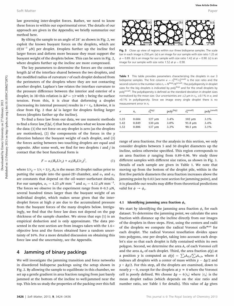
Table 1 This table provides parameters characterizing the droplets in our 3bidisperse samples. The first column s ¼ r (big)0 /r (small)

0 is the size ratio and thesecond column is the number ratio nr¼N(big)/N(small). The polydispersity in dropletsizes for the big droplets is indicated by poly(big) and for the small droplets bypoly(small). The polydispersity is defined as the standard deviation in droplet sizesnormalized by the mean size. Our uncertainties are �2 mm in r0, �0.1% in s, and<0.1% in polydispersity. Since we image every single droplet there is nomeasurement error in nr

s nr r(big)0 poly(big) r(small)0 poly(small)

1.25 0.684 127 mm 3.4% 102 mm 3.1%1.42 0.849 130 mm 3.0% 91.8 mm 3.4%1.52 0.806 137 mm 3.3% 90.1 mm 3.1%

Fig. 3 Close up view of regions within our three bidisperse samples. The scalebar in each image is 250 mm. (a) is an image for our sample with size ratio 1.25 atf ¼ 0.89. (b) is an image for our sample with size ratio 1.42 at f ¼ 0.90. (c) is animage for our sample with size ratio 1.52 at f ¼ 0.90.

Soft Matter Paper

Dow

nloa

ded

by E

mor

y U

nive

rsity

on

27 F

ebru

ary

2013

Publ

ishe

d on

13

Febr

uary

201

3 on

http

://pu

bs.r

sc.o

rg |

doi:1

0.10

39/C

3SM

2728

7GView Article Online

law governing inter-droplet forces. Rather, we need to knowthese forces to within our experimental error. The details of ourapproach are given in the Appendix; we briey summarize ourmethod here.

By tilting the sample to an angle of 28� as shown in Fig. 2, weexploit the known buoyant forces on the droplets, which areO(10�3 mN) per droplet. Droplets further up the incline feellarger forces and deform more because they must support thebuoyant weight of the droplets below. This can be seen in Fig. 2,where droplets further up the incline are more compressed.

The key parameters to determine the forces are the contactlength Dl of the interface shared between the two droplets, andthe modied radius of curvature r of each droplet deduced fromthe perimeters of the droplets where they are not contactinganother droplet. Laplace's law relates the interface curvature tothe pressure difference between the interior and exterior of adroplet; in 3D this relation is DP ¼ g/r with g being the surfacetension. From this, it is clear that deforming a droplet(increasing its internal pressure) results in r < r0. Likewise, it isclear from Fig. 2 that Dl is larger for droplets feeling largerforces (droplets farther up the incline).

To nd a force law from our data, we use numeric methodsto nd a force law f (Dl, r) that best satises what we know aboutthe data: (1) the net force on any droplet is zero (as the dropletsare motionless), (2) the components of the forces in the ydirection balance the buoyant weight of each droplet, and (3)the forces acting between two touching droplets are equal andopposite. Aer some work, we nd for two droplets i and j incontact that the best functional form is

F ¼ a1(R0L/rij) + a2(R0L/rij)2, (1)

where 1/rij ¼ 1/ri + 1/rj, R0 is the mean 3D droplet radius prior toputting the sample into the quasi-2D chamber, and a1 and a2

are constants that depend on the oil–water–surfactant details.For our samples, a1 ¼ 4.25 mN mm�1 and a2 ¼ 4.12 mN mm�2.The forces we observe in the experiment range from 0–0.5 mN,several hundred times larger than the buoyant weight of anindividual droplet, which makes sense given that the inter-droplet forces at high f are due to the accumulated pressurefrom the buoyant forces of the many droplets below. Intrigu-ingly, we nd that the force law does not depend on the gapthickness of the sample chamber. We stress that eqn (1) is anempirical deduction and is only approximate. The data pre-sented in the next section are from images taken with the 1.6�objective lens and the forces obtained have a random uncer-tainty of 16%. For a more detailed discussion on obtaining thisforce law and the uncertainty, see the Appendix.

4 Jamming of binary packings

We will investigate the jamming transition and force networksin disordered bidisperse packings using the setup shown inFig. 2. By allowing the sample to equilibrate in this chamber, weset up a gentle gradient in area fraction ranging from just barelyjammed at the bottom of the incline to well-jammed near thetop. This lets us study the properties of the packing over this full

3426 | Soft Matter, 2013, 9, 3424–3436

range of area fractions. For the analysis in this section, we onlyconsider droplets between 5 and 50 droplet diameters up theincline, unless otherwise specied. This region corresponds toan area fraction f ranging from 0.89–0.96. We study threedifferent samples with different size ratios, as shown in Fig. 3.Details of each sample are given in Table 1. We note thatmoving up from the bottom of the droplet pile, within in therst ve particle diameters the area fraction increases above thejamming point by 0.03 (see next section for jamming point), andit is plausible our results may differ from theoretical predictionsvalid for f / fc.

4.1 Identifying jamming area fraction fc

We start by identifying the jamming area fraction fc for eachdataset. To determine the jamming point, we calculate the areafraction with distance up the incline directly from our imagesof the droplets in three steps. First, using the centers and radiiof the droplets we compute the radical Voronoi cells40,41 foreach droplet. The radical Voronoi tessellation divides spaceinto polygons, one per droplet, taking into account each drop-let's size so that each droplet is fully contained within its ownpolygon. Second, we determine the area Av of each Voronoi celland the area Ad of each droplet. Third, the area fraction f(y) ata position y is computed as f(y) ¼ P

kAd,k/P

kAv,k, where kindexes all droplets with a center of mass within y � Dy/2 andy + Dy/2. For this step, all the droplets are examined, down tonearly y ¼ 0, except for the droplets at y z 0 where the Voronoicell is poorly dened. We choose Dy ¼ 6hr0i where hr0i is themean droplet radius (which depends on the size ratio andnumber ratio, see Table 1 for details). This value of Dy gives

This journal is ª The Royal Society of Chemistry 2013

Fig. 4 (a) Scatter plot of coordination number against ftheory � fc. All data werefitted together to z � zc ¼ A(f � fc)

bz, where the fit is shown as the black dashedline with fit parameters zc ¼ 4.2, A ¼ 3.2, and bz ¼ 0.4. Fitting the differentdatasets separately gives slightly different fit values, listed in Table 2. Inset of (a):scatter plot of coordination number and experimental area fraction f. The dashedline is a linear fit to all the data with slope 9.6 � 0.1 and zc ¼ 4.82 � 0.02. Thedifferent value of zc between (a) and the inset to (a) is due to the differentextrapolation function. (b) A scatter plot between pressure and ftheory � fc. Thepressure has been scaled by c ¼ 1;

ffiffiffiffiffiffi10

p, and 10 for the s ¼ 1.25, 1.42, and 1.52

data respectively. Each dataset is fitted to P ¼ A(ftheory� fc)bP, shown as the black

dashed lines. The fit values are given in Table 2. Inset of (b): scatter plot of pressureand experimental area fraction.

Table 2 The fitting parameters for the power law fits to the data for each sizeratio s. Note that simulations8 found bP ¼ bf; see text for a discussion. Theuncertainties in the fit values are obtained by computing the standard error ineach fitting parameter

z � zc ¼ Az(ftheory � fc)bz

s Az bz zc

1.25 3.2 � 0.6 0.4 � 0.2 4.3 � 0.31.42 3.3 � 0.6 0.4 � 0.2 4.3 � 0.31.52 3.2 � 0.7 0.3 � 0.2 4.0 � 0.4

P ¼ AP(ftheory � fc)bP

s AP [mN mm�1] bP

1.25 19 � 1 1.41 � 0.031.42 15 � 1 1.30 � 0.031.52 13 � 2 1.26 � 0.07

fij ¼ F0(drij/dij)bf

s F0 [mN] bf

1.25 2.3 � 0.2 1.27 � 0.031.42 2.4 � 0.1 1.19 � 0.021.52 2.0 � 0.1 1.15 � 0.03

Paper Soft Matter

Dow

nloa

ded

by E

mor

y U

nive

rsity

on

27 F

ebru

ary

2013

Publ

ishe

d on

13

Febr

uary

201

3 on

http

://pu

bs.r

sc.o

rg |

doi:1

0.10

39/C

3SM

2728

7GView Article Online

roughly 150 droplets per y sampled. Within this window of Dy,Df ¼ (vf/vy)Dy z 0.007. From f(y) we can obtain the jammingpoint fc by extrapolating the value of f to y ¼ 0, where y ¼ 0 isdened as the bottom of the droplet pile. We can treat they ¼ 0 point in our data as the jamming point since the forcesbetween droplets at y ¼ 0 are nearly zero. For the three data-sets, the extrapolation is done by tting f(y) to a power law[f(y) ¼ fc + ayb] giving fc ¼ 0.855 � 0.005, 0.861 � 0.005, and0.858 � 0.008 for the data with size ratio s ¼ 1.25, 1.42, and1.52, respectively. We chose to use f(y) ¼ fc + ayb since f � fc

vs. y appears fairly linear on a log–log plot. In simulations onfrictionless disks and experiments on 2D foams it has beenreported that fc � 0.84 for bidisperse systems,7,11,39 which is alittle lower than the values we found.

Our measured area fraction depends on where we dene theouter perimeter of a droplet. As seen in Fig. 3, the droplets havethick black outlines. We look at the outer edge of each outline,and dene the perimeter as the pixel location where theintensity is halfway between the white color outside the droplet,and the black color in the darkest part of the outline. Thetransition from black to white occurs over a distance of 2–3pixels, and so we judge that we have a systematic uncertainty inthe area fraction of roughly 1% due to the determination of theperimeter position. Since this is systematic, the distance to thejamming point (f � fc) is insensitive to this error and thereforein most of our results we focus on f � fc.

4.2 Critical scaling

The rst critical scaling we investigate is the coordinationnumber, the mean number of contacts each droplet has. Priornumerical studies of jamming in frictionless systems found thatthe coordination number z obeys a power law scaling of theform z� zc ¼ A(f� fc)

bz, where A� 3.5, zc ¼ 4, and bz¼ 1/2.5–7 Ithas been observed that A has a slight dependence on the forcelaw and polydispersity, but zc ¼ 4 and b ¼ 1/2 are independentof the force law and polydispersity. Katgert and van Hecke11

found for a 2D bidisperse foam with size ratio 1.5 a criticalscaling with A ¼ 4.02 � 0.02 and bz ¼ 0.50 � 0.02 while xingzc ¼ 4. The critical point zc has been interpreted as the isostaticpoint ziso (minimum number of contacts necessary for amechanically stable packing). For 2D, ziso ¼ 4, in agreementwith zc found in prior work.

To compare experimental data and simulation data, theexperimental area fraction needs to be converted into a theo-retical area fraction.11 This is because the simulated particlesare allowed to overlap (thus diminishing the total area they takeup at large f) while our experimental droplets always occupy thesame total area. We convert our experimental f values to ftheory

using the method of Katgert and van Hecke.11 From our data wedetermine z and ftheory at various points along the incline. Theresults are plotted relative to the jamming point in Fig. 4(a), andshow power-law scaling. Fitting the each dataset to the theo-retical scaling law, z� zc¼ A(f� fc)

bz, we obtain values for A, zc,and bz which are reported in Table 2. Our values of A z 3.2 areclose to Az 3.5 found in a numerical study by O'Hern et al.7 forparticles with size ratio 1.4. The tted values for zc are within theuncertainty of the previously found value of 4.5–7,11 However, our

This journal is ª The Royal Society of Chemistry 2013 Soft Matter, 2013, 9, 3424–3436 | 3427

Soft Matter Paper

Dow

nloa

ded

by E

mor

y U

nive

rsity

on

27 F

ebru

ary

2013

Publ

ishe

d on

13

Febr

uary

201

3 on

http

://pu

bs.r

sc.o

rg |

doi:1

0.10

39/C

3SM

2728

7GView Article Online

droplets have a slight attraction which may result in a slightlytighter packing of droplets at fc with a coordination number zc> 4. Given our uncertainties of zc, our data are consistent withboth zc ¼ 4 and zc > 4. Finally, for each packing, the exponent bzz 0.4 agrees with the prior ndings (b ¼ 0.5) to within ouruncertainty, although we have a fairly large uncertainty in ourexponents. Interestingly, in 2D photoelastic disk experiments,they found z � zc ¼ A(f � fc)

bz with bz ¼ 0.53 � 0.03 withoutneeding to convert their experimental f to ftheory,10 but A � 25for that study which is considerably different from our results.In their work, they were limited to area fractions close to fc dueto the difficulty of compressing their particles to high areafractions, while our data (and those of ref. 11) extend over alarger range of f.

The second critical scaling we investigate is the dependenceof pressure P with distance to the jamming point. Simulationsof 2D particles found P ¼ A(ftheory � fc)

bP, where A and bP

depend on the form of the force law. In the numerical study byO'Hern et al.,8 they used frictionless disks that interacted via theforce law fij ¼ F0(drij/dij)

bf, where F0 is a scale, drij is the overlapbetween two particles in contact, and dij is the sum of the radiiof the particles in contact. They found that bP ¼ bf. It is certainlypossible that for other force laws, the scaling of pressure with (f� fc) could be different. In particular, in our experiment, theforce between two droplets is not a unique function of drij butrather depends on the droplet perimeters which are inuencedby all of their neighbors. In 2D photoelastic disk experiments bPwas found to be 1.1.10 No prior experimental 2D studies haveexamined the scaling of P for systems without static friction.

For our experiment, we compute the local pressure of oursample by rst locating a set of droplets k within a window y �Dy/2 and y + Dy/2. For these k droplets the pressure is P ¼P

iP

j>iFijrij/P

kAk,v, where i and j index all contacts on the kdroplets and

PkAk,v is the sum of the Voronoi areas of all k

Fig. 5 The average force between droplets in contact plotted against theamount of compression between the droplets. The average force has been scaledby a prefactor of c ¼ 1;

ffiffiffiffiffiffi10

p, and 10 for the s ¼ 1.25, 1.42, and 1.52 data

respectively. Each data is fitted to hfiji ¼ F0(drij/dij)bf and the fits are shown as the

black dashed lines. The fit values are given in Table 2. Note that this data is aneffective force law, not the true force law: for a given drij/dij, different droplet pairsmay experience different contact forces. To illustrate this, we have added errorbars to the plot, where the error bars represent one standard deviation in thespread of measured contact forces at each drij/dij.

3428 | Soft Matter, 2013, 9, 3424–3436

droplets.8,42 In this formula, Fij and rij are both taken to bepositive scalars. Here we use Dy ¼ 5r0. In Fig. 4(b) we plot thepressure for all three packings against ftheory� fc. These resultsshow power-law scaling. The dashed lines are the t to P ¼A(ftheory � fc)

bP with the t values shown in Table 2. In partic-ular, we nd bP values between 1.26 and 1.41, larger than bP ¼1.1 found for photoelastic disks.10

To compare with the simulations of O'Hern et al.,8 we wish toapproximate how forces between our droplets depend on theirseparations drij. For each observed dij we nd the true force fijfrom our force law.We average all of the observations over smallwindows in dij to nd an effective average force law as a functionof dij, plotted in Fig. 5. The error bars emphasize that Fig. 5 isonly an average trend rather than the true force law. Intrigu-ingly, the averaged data follow a power law: we t each data toh fiji ¼ F0(drij/dij)

bf to obtain the power law exponent bf. The tsare shown as the black dashed lines in the gure, with t valueslisted in Table 2.

Our ts give bf < bP in contrast to the results of O'Hern et al.8

where bP ¼ bf. This equality was found for systems close to thejamming area fraction. The exponent for the pressure, bP,relates to how droplets are compacted with increasing f � fc.9

Close to fc, when f is slightly increased, droplets can avoidsignicant compression by rearranging and forming morecontacts, however, at larger f, droplets cannot form many newcontacts and must instead undergo larger compression.Therefore, at larger area fractions, the pressure increases morerapidly with f � fc than it does near the jamming point. Thisargument predicts bP > bf, in agreement with our data whichextends far from fc. While the uncertainty in each forcemeasurement is 16%, this uncertainty is unlikely to signi-cantly affect the pressure results, as the data of Fig. 4 and 5 areaverages over many forces.

4.3 Force distribution

We now consider the distribution of contact forces for eachpacking at different area fractions. Like before, we sample thecontacts forces at various points up the incline using a windowof y � Dy/2 and y + Dy/2. However, we need many contacts toobtain a good distribution of contact forces, and therefore, weuse Dy ¼ 30r0. (Over this range of Dy and for droplets at least 10diameters up the incline, Df¼ (vf/vy)Dy ¼ 0.025.) This windowsize gives roughly 2500 contacts for each y sampled. In Fig. 6(a),the circle data points show the distribution of contact forcesnormalized by themean contact force at locations with f� fc asindicated; all the data are for the s ¼ 1.25 packing. In all ourdata most forces are near or less than the mean force hfi andthat the maximum force is about 3hfi, with a somewhat expo-nential tail. The shape and magnitude of all the curves areroughly the same. All curves show a dip at small forces. Thetriangle symbols in Fig. 6(a) show the distribution of normalforces from Majmudar and Behringer,16 an experiment usingfrictional 2D photoelastic disks. In their experiment, the parti-cles were isotropically compressed to an area fraction �0.016above the critical area fraction. Our results look essentially thesame as theirs, despite the differences in experimental systems.

This journal is ª The Royal Society of Chemistry 2013

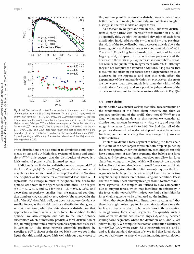
Fig. 6 (a) Distribution of contact forces relative to the mean contact force atdifferent f for the s ¼ 1.25 packing. The mean force is hfi ¼ 0.011 mN, 0.045 mN,and 0.13 mN for the f � fc ¼ 0.024, 0.062, and 0.090 data respectively. The solidtriangles are data from a 2D photoelastic disk experiment at f � fc � 0.016 fromMajmudar and Behringer.16 The solid curves are q-model fits to the data of theform P � (f/hfi)N�1exp(�Nf/hfi). The fits gave N ¼ 2.19, 3.76, and 4.21 for the f �fc ¼ 0.024, 0.062, and 0.090 data respectively. The dashed black curve is theprediction of the force network ensemble. (b) The standard deviation of P(f/hfi)for each packing at different f. The standard deviation of the Majmudar andBehringer data is 0.52.

Paper Soft Matter

Dow

nloa

ded

by E

mor

y U

nive

rsity

on

27 F

ebru

ary

2013

Publ

ishe

d on

13

Febr

uary

201

3 on

http

://pu

bs.r

sc.o

rg |

doi:1

0.10

39/C

3SM

2728

7GView Article Online

These distributions are also similar to simulations and experi-ments on 2D and 3D frictionless systems of foams and emul-sions.7,11,17,21 This suggest that the distribution of forces is afairly universal property of all jammed systems.

Additionally, we t the force distributions to the q-model26 ofthe form P � ( f/h fi)N�1exp(�Nf /hfi), where N is the number ofneighbors a transmitted load on a droplet is divided. Treatingone neighbor as the source for a transmitted load, then N + 1represents the average number of neighbors. The ts to theq-model are shown in the gure as the solid lines. The ts gaveN + 1 ¼ 3.19, 4.76, and 5.21 for the f � fc ¼ 0.024, 0.062, and0.090 data respectively, smaller than the measured coordina-tion numbers 4.9, 5.4, and 5.7 respectively. The q-model ts thetail of the P( f) data fairly well, but does not capture the data atsmaller forces, as the model predicts a distribution that goes tozero at zero force, while the data shows a distribution thatapproaches a nite value at zero force. In addition to theq-model, we also compare our data to the force networkensemble,31 which numerically predicts a force distribution atthe jamming point from similar ensemble arguments discussedin Section 4.4. The force network ensemble predicted bySnoeijer et al.31 is shown as the dashed black line. We see in thegure that this model agrees fairly well with our data closest to

This journal is ª The Royal Society of Chemistry 2013

the jamming point. It captures the distribution at smaller forcesbetter than the q-model, but our data are not clear enough todistinguish the two models at larger forces.

As observed by Katgert and van Hecke,11 our force distribu-tions slightly narrow with increasing area fraction in Fig. 6(a).To quantify this, we plot the standard deviation of each forcedistribution in Fig. 6(b). For the s¼ 1.25 and s¼ 1.42 packings,the width of the force distributions decreases quickly above thejamming point and then saturates to a constant width of �0.5.The s ¼ 1.52 packing has a broader distribution of forces atlarger f � fc compared to the other two packings, and thedecrease in the width as f� fc increases is more subtle. Overall,our results are qualitatively in agreement with ref. 11 althoughthey did not compute the standard deviations. It is possible thatmeasurement errors in our forces have a dependence on f, asdiscussed in the Appendix, and that this could affect thedependence of the standard deviation on f. However, the errorsare no worse than 16%, much less than the width of thedistributions for any f, and so a possible f-dependence of theerrors cannot account for the decrease in width seen in Fig. 6(b).

4.4 Force chains

In this section we consider various statistical measurements onthe randomness of the force chain network, and then wecompare predictions of the Brujic–Zhou model17,21,22,34 to ourdata. When analyzing data in this section we consider alldroplets and contacts between 40 # y/2r0 # 80, and over thisrange f increases from 0.93 to 0.96. We nd that all of theproperties discussed below do not depend on f at larger areafractions, and so considering this larger range of f gives usbetter statistics.

To start, we dene a force segment to belong to a force chainif it is one of the two largest forces on both droplets joined bythe force segment. Under this denition, each droplet can onlyhave a maximum of two force segments that belong to a forcechain, and therefore, our denition does not allow for forcechain branching or merging, which will simplify the analysisbelow. Note that even droplets with small forces can participatein force chains, given that the denition only requires the forcesegments to be large for the given droplet and its contactingneighbors. Fig. 7 shows force chains using our denition. Thesechains are fairly linear and vary in length from 1 tomore than 10force segments. Our samples are formed by slow compactiondue to buoyant forces, which may introduce an anisotropy inthe force chain network.16,25,43 Indeed, we nd a slight bias forforce chain segments to be orientated up the incline.

Given that force chains form linear like structures and thatthere is a slight anisotropy for force chains to align along theincline we may expect there to be correlations in the orientationof neighboring force chain segments. To quantify such acorrelation we dene two relative angles q1 and q2 betweenjoining force segments, where the denition of q1 and q2 areshown in Fig. 8. We compute the Pearson correlation coefficientC ¼ cov(q1,q2)/sq

2, where cov(q1,q2) is the covariance of q1 and q2

and sq is the standard deviation of q. We nd that for all f, C iszero or nearly zero (at most C ¼ 0.2), indicating no correlation.

Soft Matter, 2013, 9, 3424–3436 | 3429

Fig. 8 Definitions of the angles q1 and q2 between joining force segment. In thesketch both q1 (clockwise to extended line) and q2 (counter clockwise to extendedline) are positive. If there is a correlation in orientation that tends to make forcechains linear, then the correlation between q1 and q2 is positive.

Fig. 9 (a) Distribution of q for each packing, where both q1 and q2 are treated asa single variable q. The red solid line is the distribution for the s ¼ 1.25 packing,the green dashed line is the distribution for the s ¼ 1.42 packing, and the bluedashed-dot line is the distribution for the s ¼ 1.52 packing. (b–d) Comparisonsbetween the experimental distributions and the predictions of the Brujic–Zhoumodel, for size ratios (b) s ¼ 1.25, (c) s ¼ 1.42, and (d) s ¼ 1.52.

Fig. 7 This image shows only the forces belonging to a force chain within aregion of the s ¼ 1.25 sample. On average, the forces are larger further up theimage because the sample is inclined, and this can be observed in the image bythe increasing redness of the force segments at the top.

Soft Matter Paper

Dow

nloa

ded

by E

mor

y U

nive

rsity

on

27 F

ebru

ary

2013

Publ

ishe

d on

13

Febr

uary

201

3 on

http

://pu

bs.r

sc.o

rg |

doi:1

0.10

39/C

3SM

2728

7GView Article Online

This agrees with prior work on 3D emulsions.17,21 Thus, theapparent linearity of force chains seen in some locations ofFig. 7 is not due to correlations in the relative direction ofneighboring segments that would keep the chain straight.

To further explore the tendency for force chains to be linear,we consider the distribution of q1, where we drop the subscript 1as we are only focusing on two force segments at a time ratherthan three. In Fig. 9(a) we plot the distribution in q for all threepackings. The distribution shows that most force chainsegments form at an angle |q| < 60�. Thus, force segments tendto form a linear chain not because their orientations arecorrelated, but simply because it's more probable that they areoriented at small angles relative to each other. Using our P(q)data, we determine the persistence lengths l using the standarddenition of persistence length for polymer chains.

We nd l ¼ 4.4hr0i, 4.8hr0i, and 3.8hr0i for the s ¼ 1.25, 1.42,and 1.52 data. These are the distances beyond which the forcechain has “forgotten” its original direction. In analyzing thedistributions similar to P(q) for 3D emulsions, Zhou and Din-smore34 found a persistence length slightly larger around l � 6–8hr0i.

To further consider the orientations of force segments in forcechains, we consider a model proposed by Brujic et al.21,22 andextended by Zhou et al.17,34 The Brujic–Zhoumodel is amethod forgenerating ensembles of local particle congurations (a centralparticle and contacting rst neighbors) and the forces acting on a

3430 | Soft Matter, 2013, 9, 3424–3436

central particle by its rst neighbors. Each local conguration isgenerated by randomly placing zi contacting neighbors such thatany two neighboring particles do not overlap. Next, the contactforces between the central particle and zi � 2 neighboring parti-cles are chosen at random from a distribution P(f), leaving twounknown contact forces. We choose P(f) to match our experi-mentally measured distributions (see Fig. 6). By invoking forcebalance, the two remaining contact forces are found algebraically.Once a sufficient number of local congurations are generated,the distribution of force chain orientations can be studied. Thebasic assumptions of this model are force balance, randomnessin the magnitude of forces, and randomness in the orientation offorces. For our data the rst assumption applies because thesystem is in mechanical equilibrium and above we have shownthat the other two assumption reasonably apply.

One issue in using the Brujic–Zhou model to predict P(q) isthat themodel only gives the forces between a central droplet andits rst neighbors. To dene a force chain segment we also needto know all the forces acting on each rst neighbor as well. Wetherefore extend their model by generating additional forces onthe neighboring droplets in exactly the same way (constrained bythe forces already chosen for the central droplet). This lets usapply our force chain denition given above, which requires thatforce segments be among the largest two forces on both dropletsthe force acts between. We repeat this extended Brujic–Zhoualgorithm many times to compile data from all cases where thealgorithm gives an instance of two valid force segments so thatwe can determine q1. To make the inputs into the model asconsistent as possible with our experimental data, instead ofrandomly generating local congurations, we randomly selectlocal congurations from our experimental data.

Fig. 9(b)–(d) compares P(q) measured in our experiments(black solid curves) with the predictions of the model (red dot-dashed curves). The model is in good agreement with the

This journal is ª The Royal Society of Chemistry 2013

Fig. 10 Distribution of the number of force segments making up distinct forcechains. The data points are experimental values and the dashed lines are fits tothe data of the form P(n) ¼ (1 � p)pn, where p is found to be 0.722, 0.758, and0.717 for the s ¼ 1.25, 1.42, and 1.52 packings, respectively.

Paper Soft Matter

Dow

nloa

ded

by E

mor

y U

nive

rsity

on

27 F

ebru

ary

2013

Publ

ishe

d on

13

Febr

uary

201

3 on

http

://pu

bs.r

sc.o

rg |

doi:1

0.10

39/C

3SM

2728

7GView Article Online

experiment, with the exception of some discrepancies in themagnitudes of the peaks. The model captures signicantfeatures of the data: for instance, the peak around q ¼ 0� ismuch different between Fig. 9(b) and (d), and the model repli-cates this difference. We also note that if we loosen the deni-tion of force chain segments to simply those forces that are thelargest two forces acting on any droplet (independent of howlarge they are relative to forces on neighboring droplets), wend nearly identical distributions as the ones shown in Fig. 9.

Our analysis suggests so far that the force chain network israndom, without long-range correlations. It therefore seemsplausible that the distribution of force chain lengths shouldobey a random process. If there is a probability p for a forcechain segment to be connected to a neighboring force chainsegment, then the distribution of chain lengths should obey thescaling P(n) ¼ (1 � p)pn, where n is the number of forcesegments within a force chain. In Fig. 10 we plot the distribu-tion of chain lengths for each packing. The data decay expo-nentially over 3 orders of magnitude. The data are t by P(n) ¼(1 � p)pn with p z 0.73 (see caption for details), indicating thatit is highly likely that for a force chain to propagate through thematerial. The ts are shown as the dashed lines and show goodagreement with the data other than at n ¼ 1.

In granular quasi-static intruder simulations with frictionbetween particles by Peters et al., using a more sophisticateddenition of force chains, they also found an exponentialdistribution of chain lengths.44 From their reported data onP(n), we estimate a value of p ¼ 0.65. It appears that statisticallya force chain can be thought of as a random process withprobability p for the force chain to propagate, independent of fbut perhaps depending on the sample details.

5 Conclusions

We have introduced a new experimental model system composedof quasi-2D emulsions droplets to study the jamming transition.Our droplets are circular in shape and deform when pressed intoone another, and at the contacts between two droplets the forces

This journal is ª The Royal Society of Chemistry 2013

are in-plane mimicking a true 2D system. We can accuratelymeasure the forces between touching droplets to within 8%,where our method is not limited to our experiment, and could beextended to determine forces in 2D foams, 3D emulsions, and 3Dfoams. Our model system has unique strengths; we can easilymake samples with any distribution in particle sizes, emulsionsare stable over many days, setup is cheap, our droplets have nostatic friction, and our method can be extended to cases of ow.45

Using our model system we observed power-law scaling ofthe contact number and pressure with f � fc, similar to priornumerical models.5–8 Notably we nd that all three t parame-ters for the contact number scaling are quite close to the valuesfound in 2D simulations. We verify experimentally for the rsttime a link between the interparticle force law and the criticalpressure exponent, illustrating a direct relationship betweenthe bulk properties of an amorphous solid and the interactionbetween the constituent particles. The agreement of our resultsand the numerical models shows that the qualitatively differentparticle interaction we have does not play a signicant role indetermining the geometric structure and bulk modulus.

Our analysis of the inter-particle forces found a probabilitydistribution of forces in good agreement with those found inprior experiments and simulations, strongly suggesting that theshape is universal. We further examined the spatial structure ofthe large forces (“force chains”). The directions of neighboringforce chain segments are uncorrelated although there is atendency for two force chains to be in the same direction. This isa sensible result as this allows the large forces acting on a dropletto balance one another. The Brujic–Zhou model, which assumesrandom and uncorrelated force segments, recovers our experi-mentally observed probability distribution of angles betweenadjacent force segments.

This work provides more evidence for the universality ofvarious properties of the jamming transition, such as criticalscaling, the shape of the force distribution, and the structure ofthe force network.

A Method for determining force law

In this section we describe in detail our method for determiningan empirical force law that relates the outline of droplets to thecontact forces. For an overview of our method see Section 3. Thissection is organized in the followingmanner: rst, we discuss themeasurements from droplet outlines; second, we discuss thegeneral form of possible force laws; third, we present the opti-mization problem; fourth, we deduce the best force law consis-tent with the data.

A.1 Measurable variables

In this subsection, we discuss the various quantities measur-able from droplet images, and their measurement errors. In thefollowing subsections, these quantities will be used to deter-mine the forces between droplet pairs.

The larger the contact between two droplets, the more forcethey feel. This is quantied by the contact length lij between twodroplets. We measure this by identifying the portion of each

Soft Matter, 2013, 9, 3424–3436 | 3431

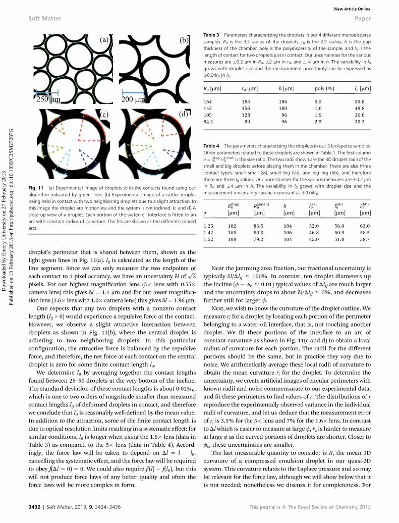
Fig. 11 (a) Experimental image of droplets with the contacts found using ouralgorithm indicated by green lines. (b) Experimental image of a rattler dropletbeing held in contact with two neighboring droplets due to a slight attraction. Inthis image the droplet are motionless and the system is not inclined. (c and d) Aclose up view of a droplet. Each portion of the water–oil interface is fitted to anarc with constant radius of curvature. The fits are shown as the different coloredarcs.

Table 3 Parameters characterizing the droplets in our 4 different monodispersesamples. R0 is the 3D radius of the droplets, r0 is the 2D radius, h is the gapthickness of the chamber, poly is the polydispersity of the sample, and l0 is thelength of contact for two droplets just in contact. Our uncertainties for the variousmeasures are �0.2 mm in R0, �2 mm in r0, and � 4 mm in h. The variability in l0grows with droplet size and the measurement uncertainty can be expressed as�0.04r0 in l0

R0 [mm] r0 [mm] h [mm] poly (%) l0 [mm]

164 183 186 5.5 50.8143 156 180 1.6 48.8105 128 96 1.9 36.684.1 89 96 2.5 30.3

Table 4 The parameters characterizing the droplets in our 3 bidisperse samples.Other parameters related to these droplets are shown in Table 1. The first columns¼ r(big)0 /r(small)

0 is the size ratio. The two radii shown are the 3D droplet radii of thesmall and big droplets before placing them in the chamber. There are also threecontact types: small–small (ss), small–big (sb), and big–big (bb), and thereforethere are three l0 values. Our uncertainties for the various measures are �0.2 mmin R0 and �4 mm in h. The variability in l0 grows with droplet size and themeasurement uncertainty can be expressed as �0.04r0

s

R(big)0

[mm]R(small)0

[mm]h[mm]

l(ss)0

[mm]l(sb)0

[mm]l(bb)0

[mm]

1.25 102 86.5 104 52.0 56.0 63.01.42 105 80.0 106 46.8 50.9 58.51.52 108 79.2 104 45.0 51.0 58.7

Soft Matter Paper

Dow

nloa

ded

by E

mor

y U

nive

rsity

on

27 F

ebru

ary

2013

Publ

ishe

d on

13

Febr

uary

201

3 on

http

://pu

bs.r

sc.o

rg |

doi:1

0.10

39/C

3SM

2728

7GView Article Online

droplet's perimeter that is shared between them, shown as thelight green lines in Fig. 11(a). lij is calculated as the length of theline segment. Since we can only measure the two endpoints ofeach contact to 1 pixel accuracy, we have an uncertainty dl of

ffiffiffi2

ppixels. For our highest magnication lens (5� lens with 0.55�camera lens) this gives dl ¼ 1.1 mm and for our lower magnica-tion lens (1.6� lens with 1.0� camera lens) this gives dl¼ 1.96 mm.

One expects that any two droplets with a nonzero contactlength (lij > 0) would experience a repulsive force at the contact.However, we observe a slight attractive interaction betweendroplets as shown in Fig. 11(b), where the central droplet isadhering to two neighboring droplets. In this particularconguration, the attractive force is balanced by the repulsiveforce, and therefore, the net force at each contact on the centraldroplet is zero for some nite contact length l0.

We determine l0 by averaging together the contact lengthsfound between 25–50 droplets at the very bottom of the incline.The standard deviation of these contact lengths is about 0.025r0,which is one to two orders of magnitude smaller than measuredcontact lengths lij of deformed droplets in contact, and thereforewe conclude that l0 is reasonably well-dened by the mean value.In addition to the attraction, some of the nite contact length isdue to optical resolution limits resulting in a systematic effect: forsimilar conditions, l0 is longer when using the 1.6� lens (data inTable 3) as compared to the 5� lens (data in Table 4). Accord-ingly, the force law will be taken to depend on Dl ¼ l � l0,cancelling the systematic effect, and the force law will be requiredto obey f(Dl ¼ 0) ¼ 0. We could also require f (l) � f(l0), but thiswill not produce force laws of any better quality and oen theforce laws will be more complex in form.

3432 | Soft Matter, 2013, 9, 3424–3436

Near the jamming area fraction, our fractional uncertainty istypically dl/Dlij z 100%. In contrast, ten droplet diameters upthe incline (f � fc z 0.01) typical values of Dlij are much largerand the uncertainty drops to about dl/Dlij z 5%, and decreasesfurther still for larger f.

Next, we wish to know the curvature of the droplet outline. Wemeasure ri for a droplet by locating each portion of the perimeterbelonging to a water–oil interface, that is, not touching anotherdroplet. We t these portions of the interface to an arc ofconstant curvature as shown in Fig. 11(c and d) to obtain a localradius of curvature for each portion. The radii for the differentportions should be the same, but in practice they vary due tonoise. We arithmetically average these local radii of curvature toobtain the mean curvature ri for the droplet. To determine theuncertainty, we create articial images of circular perimeters withknown radii and noise commensurate to our experimental data,and t these perimeters to nd values of r. The distributions of rreproduce the experimentally observed variance in the individualradii of curvature, and let us deduce that the measurement errorof ri is 3.5% for the 5� lens and 7% for the 1.6� lens. In contrasttoDlwhich is easier tomeasure at large f, rc is harder tomeasureat large f as the curved portions of droplets are shorter. Closer tofc, these uncertainties are smaller.

The last measurable quantity to consider is �R, the mean 3Dcurvature of a compressed emulsion droplet in our quasi-2Dsystem. This curvature relates to the Laplace pressure and somaybe relevant for the force law, although we will show below that itis not needed; nonetheless we discuss it for completeness. For

This journal is ª The Royal Society of Chemistry 2013

Fig. 12 An experimental image of a mineral oil droplet squeezed between twoglass slides, where the gap thickness is 1 mm, Ri,k ¼ 0.88 mm and Ri,t ¼ 0.56 mm.The orange (light) dashed line is a fit to the perimeter to obtain Ri,k and Ri,t.

Paper Soft Matter

Dow

nloa

ded

by E

mor

y U

nive

rsity

on

27 F

ebru

ary

2013

Publ

ishe

d on

13

Febr

uary

201

3 on

http

://pu

bs.r

sc.o

rg |

doi:1

0.10

39/C

3SM

2728

7GView Article Online

scenarios where droplets are asymmetrically deformed in 3D, thewater–oil interface has two principle radii, the maximum radiusof curvature Ri,1 and the minimum radius of curvature Ri,2. Fordroplets compressed in this manner, the mean curvature 1/�Ri ¼1/2(1/Ri,1 + 1/Ri,2) is constant anywhere on the surface.

To measure Ri,1 and Ri,2 experimentally we take side viewimages of isolated droplets in a sample chamber of gap thicknessh ¼ 1 mm (see Fig. 12). The width of the droplet cross-section is2Ri,1, and Ri,1 corresponds to the droplet radius that would bemeasured as the 2D radius in the normal top-down view of ourexperiments. The free surface of this compressed droplet is asurface of mean curvature �R; this is not a circular arc of constantradius as R1 varies with height. To obtain Ri,1 and Ri,2 of thedroplet, we t the surface using the method of Caboussat andGlowinski46 (an algorithm to generate the surface of a dropletcompressed between two boundaries). In Fig. 12, we show the tas the orange dashed line. Repeating this method for manydroplets, we nd Ri,t/h ¼ 0.552 � 0.011 for droplets in the sizerange we use. For simplicity, we simply use Ri,t¼ 0.552h for all ri.

A.2 Mathematical treatment of an empirical force law

Our goal is to nd an empirical force law f(lij,l0,ri,rj) relating thecontact force between two droplets i and j to the informationabout their outlines. A priori it is useful to consider what such aforce law should look like.

We rst consider two cases where the force law is alreadyknown, the ideal 2D case and the ideal 3D case. By ideal, wemean that the contact angle between two droplets is zero, andwhere there are no attractive forces. Generally these are notrealistic assumptions, due to the interactions between thesurfactant molecules at the contacting interface.47,48 For theideal cases, the force between two droplets in contact can bemodeled using Princen's 2D model49–51 or Zhou's 3D model.52

We use lower case to indicate 2D variables and upper case toindicate 3D variables. In 2D, the contact between two dropletshas a contact length lij, and in 3D, the contact has contact areaAij. The force law for the two models are

2D Model : fij ¼ g2D

lij

rij; where rij ¼ ri þ rj

rirj(2)

3D Model:Fij ¼ g3D

Aij

Rij

; whereRij ¼ Ri þ Rj

RiRj

(3)

In the above equations, g2D is a 2D line tension and g3D is a3D surface tension. For scenarios where droplets are

This journal is ª The Royal Society of Chemistry 2013

asymmetrically deformed in 3D, the radius of curvature Rij inthe 3D model must be replaced by the mean curvature �Rij. Notethat in the above expressions, the force laws do not explicitlydepend on the center to center distance between two droplets.Starting from similar physical arguments that led to eqn (3),Mason et al.12 derived an approximate force law dependinglinearly on the center to center distance of two droplets, whichallowed them to correctly model the dependence of the samplemodulus on volume fraction. At larger compressions, the rela-tionship is non-linear, and in the work Lacasse et al.53 theymeasured this non-linearity. They found that the exact form ofthe force law slightly depended on the number of neighbors andhow the neighboring droplets are arranged. This is because thenumber of neighbors and their positions modies the radius ofcurvature of a droplet, which should be the more fundamentalquantity (as it relates to the Laplace pressure within a droplet).Accordingly, we focus our search for force laws of forms similarto eqn (2) or eqn (3).

The 2D model would be straightforward to apply as wedirectly measure lij, ri, and rj. To apply the 3D model, areasonable assumption is that Aij is related to lij and perhaps thedroplet radii. The radii �Ri and �Rj are measurable as described inthe previous subsection.

Rather than choosing between the 2D and 3Dmodels, we testgeneralizations of both models and let the data select whatworks best. As described above, one of our variables the forcewill depend on is Dlij and we constrain all possible force laws sothat f(Dlij ¼ 0) ¼ 0. In general, we consider models of the formf(2D)ij (Dlij,1/rij;~a) for 2D and f(3D)ij (Dlij,1/�Rij;~a) for 3D.~a ¼ a1,a2,.are the tting parameters associated with a given functionalform. To give an example, we could write f2Dij ¼ a1(Dlij/rij)

a2 withtting parameters a1 and a2. In all, we test a total of 86 various2D and 3D force laws of different functional forms that includeexponentials, hertzians, power laws, and polynomials in lij, 1/rij,and 1/�Rij, and combinations of these forms.

A.3 Optimization problem

To test the force laws, we establish constraints from the data,optimize each force law subject to the constraints, and thenquantify how well the optimum force laws describe the data. Tostart with, we consider the constraints on forces in the x and ydirections.

In the y-direction the sum of the forces on any given dropletis equal to the buoyant weightWD. This is in practice hard to usedirectly, as WD is small compared to the contact forces, andlikely below limits set by noise. Therefore, rather than consid-ering individual droplets, we note that droplets located at agiven y must support the observed total buoyant weight Wobs ofdroplets below them, known simply from measuring the totalarea of droplets with centers below y. The way in which thesedroplets support this buoyant weight is through contact forces,and for an assumed force law fij(Dlij,1/rij; ~a) we can determinethese contact forces by substituting our measured values for Dlijand rij (or �Rij) into the function. If the assumed force modelaccurately predicts the forces, then the sum of these contactforces

PFmod,y at a given y will equalWobs. Here

PFmod,y are the

Soft Matter, 2013, 9, 3424–3436 | 3433

Soft Matter Paper

Dow

nloa

ded

by E

mor

y U

nive

rsity

on

27 F

ebru

ary

2013

Publ

ishe

d on

13

Febr

uary

201

3 on

http

://pu

bs.r

sc.o

rg |

doi:1

0.10

39/C

3SM

2728

7GView Article Online

sum of the y-component of only those forces pointed in thedownward directions. The reason we only consider the down-ward facing forces is because the collective buoyant weight ispushing upward, and to satisfy Newton's 3rd law, the balancingforces must be facing downward. We convert Wobs and Fmod,y

into 2D pressures (force per unit length) by writing lobs ¼ Wobs/w, lmod ¼

PFmod,y/w, using the width of the chamber w. l is in

essence the 2D hydrostatic pressure at height y. Because there isno static friction at the sidewalls, there is no Janssen effect.54

We dene a goodness of comparison in the y-direction as

cy2 ¼

Xy

��lðyÞobs � lðyÞmod

���lðyÞobs

�2; (4)

where smaller values of cy2 indicate a better match between the

assumed force law and the actual forces. In the equation, yindexes various distances up the incline where l(y)mod andl(y)obs are sampled, and the angle brackets are an average overy. We normalize by hl(y)obsi to make cy

2 dimensionless, andsince hl(y)obsi is independent of the assumed force law, it doesnot change the results. We sample l at intervals of 5r0 up theincline. At each y sampled, lmod is calculated using the contactlengths and droplet radii for all droplets found between adistance y � 5r0 and y + 5r0 up the incline, and lobs is calculatedusing the position and radii of all droplets below a distance y upthe incline.

We next consider the forces in the x-direction. In contrast tothe y-direction there are no external forces, so the sum of theforces on each droplet in the x-direction is zero. From this weconstruct the goodness of comparison

cx2 ¼

Xi

" Xj

fx;ij

!,D~f iE#2; (5)

where the Fx,ij is the x component of the force at a contactbetween droplets i and j and h|~f i|i is the average net contactforce exerted on droplet i. In the equation, fx,ij are the forcespredicted by the assumed force law. Due to measurement error,the forces will not sum to zero, and the deviation from zerogrows with h|~f i|i. We assume that the deviation will grow line-arly with h|~f i|i and to fairly weight the contributions of eachdroplet to cx

2, we normalize the sum of the forces by h|~f i|i.Finally, we dene a net goodness of comparison c2 ¼ cx

2cy2

which indicates how well an assumed force law models theforces in both the x and y directions. Since we know the buoyantweight of our droplets in units of mN, this allows us to nd aforce law in units of mN. Later, we compare c2 between thedifferent force laws to determine the best overall force law.

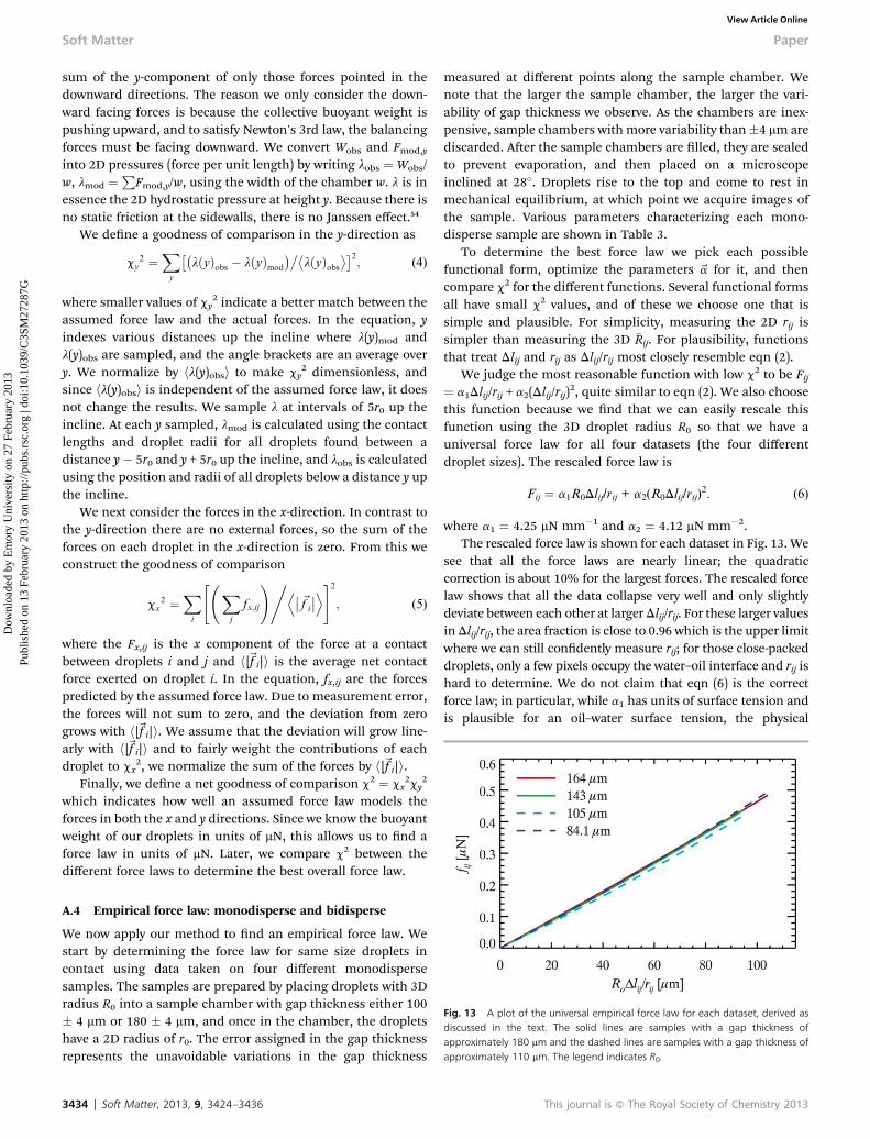
Fig. 13 A plot of the universal empirical force law for each dataset, derived asdiscussed in the text. The solid lines are samples with a gap thickness ofapproximately 180 mm and the dashed lines are samples with a gap thickness ofapproximately 110 mm. The legend indicates R0.

A.4 Empirical force law: monodisperse and bidisperse

We now apply our method to nd an empirical force law. Westart by determining the force law for same size droplets incontact using data taken on four different monodispersesamples. The samples are prepared by placing droplets with 3Dradius R0 into a sample chamber with gap thickness either 100� 4 mm or 180 � 4 mm, and once in the chamber, the dropletshave a 2D radius of r0. The error assigned in the gap thicknessrepresents the unavoidable variations in the gap thickness

3434 | Soft Matter, 2013, 9, 3424–3436

measured at different points along the sample chamber. Wenote that the larger the sample chamber, the larger the vari-ability of gap thickness we observe. As the chambers are inex-pensive, sample chambers with more variability than�4 mm arediscarded. Aer the sample chambers are lled, they are sealedto prevent evaporation, and then placed on a microscopeinclined at 28�. Droplets rise to the top and come to rest inmechanical equilibrium, at which point we acquire images ofthe sample. Various parameters characterizing each mono-disperse sample are shown in Table 3.

To determine the best force law we pick each possiblefunctional form, optimize the parameters ~a for it, and thencompare c2 for the different functions. Several functional formsall have small c2 values, and of these we choose one that issimple and plausible. For simplicity, measuring the 2D rij issimpler than measuring the 3D �Rij. For plausibility, functionsthat treat Dlij and rij as Dlij/rij most closely resemble eqn (2).

We judge the most reasonable function with low c2 to be Fij¼ a1Dlij/rij + a2(Dlij/rij)

2, quite similar to eqn (2). We also choosethis function because we nd that we can easily rescale thisfunction using the 3D droplet radius R0 so that we have auniversal force law for all four datasets (the four differentdroplet sizes). The rescaled force law is

Fij ¼ a1R0Dlij/rij + a2(R0Dlij/rij)2. (6)

where a1 ¼ 4.25 mN mm�1 and a2 ¼ 4.12 mN mm�2.The rescaled force law is shown for each dataset in Fig. 13. We

see that all the force laws are nearly linear; the quadraticcorrection is about 10% for the largest forces. The rescaled forcelaw shows that all the data collapse very well and only slightlydeviate between each other at largerDlij/rij. For these larger valuesinDlij/rij, the area fraction is close to 0.96 which is the upper limitwhere we can still condently measure rij; for those close-packeddroplets, only a few pixels occupy the water–oil interface and rij ishard to determine. We do not claim that eqn (6) is the correctforce law; in particular, while a1 has units of surface tension andis plausible for an oil–water surface tension, the physical

This journal is ª The Royal Society of Chemistry 2013

Paper Soft Matter

Dow

nloa

ded

by E

mor

y U

nive

rsity

on

27 F

ebru

ary

2013

Publ

ishe

d on

13

Febr

uary

201

3 on

http

://pu

bs.r

sc.o

rg |

doi:1

0.10

39/C

3SM

2728

7GView Article Online

meaning of a2 is unclear. Rather, eqn (6) accurately provides theforces between our droplets, within the measurement limitationsset by our data. Also, there may be other sources of error; forinstance, Lacasse et al.53 has numerically shown that the force lawhas a slight sensitivity to the number of neighbors and the rela-tive positioning of the neighboring droplets. To examine if thereare other potential sources of error, using eqn (6) we comparedthe deviations in the computed net force on each droplet to thedeviations we expect given our measurement errors, and nd thetwo agree well. Thus, within the limitations of our measurementerrors, we have resolved the forces as best as possible, conrmingeqn (6) is adequate.

To test how well one can determine a force law given nitedata and measure error, we additionally simulated inclinedmechanically stable droplet packings of 1000 droplets with aknown force law, then added noise to the data consistent withexperimental noise. Applying our empirical method to thesimulated data, we recover the known force law with 2% errorsin the coefficients (noise equivalent to the experiments usingthe 5� microscope objective) or 5% errors in the coefficients(noise equivalent to the experiments with the 1.6� microscopeobjective). This suggests it is possible that the �4% variationsbetween the force laws for different sized droplets seen inFig. 13 are simply due to noise, and they may well have exactlythe same force law.

So far we have focused on force laws in monodispersesamples, but we also need to measure forces between different-sized droplets in bidisperse samples. To obtain a force lawbetween droplets of different sizes, we apply our method to ndan empirical force law using data taken on three differentbidisperse samples. The bidisperse samples are prepared in thesame manner as the monodisperse case. Table 4 summarizes thevarious parameters of our bidisperse systems; see also Table 1.

For the case of a bidisperse sample with small and bigdroplets, there are 3 possible contact types to consider: small–small, small–big, and big–big. Our previous results give ussmall–small and big–big forces. We assume the unknownsmall–big force law obeys the same functional form as themonodisperse case (eqn (6)), where a1 and a2 need to bedetermined. Recall that eqn (6) contains a term R0 that rescalesthe force law and makes it universal. For the small–big contactsthere are two different R0 values, one for each droplet size. Toaccount for these two radii we substitute R0 with the arithmeticmean of the two radii hR0i giving as our bidisperse empiricalforce law Fij ¼ a1hR0iDlij/rij + a2(hR0iDlij/rij)2, where a1 and a2 areunknown. To obtain a1 and a2 for our bidisperse samples weminimize c2, and nd that a1 and a2 are very close to that foundfor the monodisperse case and within the 4% variation weexpect from nite sampling and measurement error. Therefore,we have shown that to within 5% error we have a found auniversal force law that works for any droplet size and is close toPrincen's 2D model49–51 with a small second order correction.

A.5 Final comments on force law

The uncertainties in determining forces are related to themagnication. The higher the magnication, the better we can

This journal is ª The Royal Society of Chemistry 2013

measure the contact length l and the mean curvature r. Fortu-nately, given that we study static samples, this means we cantake overlapping images at high magnication to reduce ouruncertainties, as described in Section 2. In an experiment withmoving droplets, overlapping images of different elds of viewwould be difficult or impossible. This situation would requirelimiting the eld of view to fewer droplets, if the same resolu-tion of forces was desired. For any magnication, uniformity oflighting is essential so that the appearance of droplets isuniformly related to their true shape and size. As discussed inthe previous subsection, our imperfect knowledge of the forcelaw gives us a systematic uncertainty no worse than 5%. Todetermine the random uncertainty for particular forces, we takemeasured rij and Dlij values, add noise commensurate to ourknown uncertainty (discussed in Section A.1), and recalculatethe force to see the variation. The bidisperse data of Section 4were taken with a 1.6� lens and have a random uncertainty of16%. The monodisperse data used in the calibration procedurewere taken with a 5� lens and have a random uncertainty of 8%.

An additional experimental complication is that droplets atrest occasionally feel a static force from the top and bottomplates. This is likely due to contact line pinning on impurities ormicroscopic scratches on the glass. To minimize this, we pre-clean each slide with methanol which we gently blow off theslide. Harsher cleaning methods do not signicantly reduce thedroplet pinning. The magnitude of these forces can be esti-mated by examining a dilute concentration of droplets in ahorizontal slide, and then slowly tilting the slide to see when thedroplets begin to move due to gravity. For the samples dis-cussed in this work, they begin to move at tilt angles of about4.5� or sooner. We discard any sample chambers with pinningstronger than this. Given that our experiments are conducted ata tilt angle of 28�, the buoyant weight of a droplet is sin(28�)/sin(4.5�) ¼ 6 times larger than any pinning force. Taking theanalysis a little further, since the friction force on any dropletcan range from zero to the maximum, a more appropriateestimate for the buoyant weight of a droplet is sin(28�)/(sin(4.5�)/2) ¼ 12 times the average pinning force. These esti-mates show that the inter-droplet forces seen in the jammedemulsions (f > fc) are on the order of a hundred times thepinning forces. We believe that the situation in our calibrationexperiments are even more favorable. Aer compaction, thepinning forces should be in random directions, as an analogousgranular experiment observed that particles move in randomdirections during compaction.55 Therefore, a vector averagegives a pinning force on each droplet very close to zero. Sinceour empirical method relies on the average vector forces on adroplet, the pinning forces can safely be neglected in the resultsof Section 4. Note that if our experiment was scaled down in size(smaller droplets, thinner plate gap) the pinning forces becomemore signicant compared to the droplet weight and candominate the results.

Acknowledgements

We thank G. Hunter and G. Hentschel for helpful discussions.This work was supported by the donors of The Petroleum

Soft Matter, 2013, 9, 3424–3436 | 3435

Soft Matter Paper

Dow

nloa

ded

by E

mor

y U

nive

rsity

on

27 F

ebru

ary

2013

Publ

ishe

d on

13

Febr

uary

201

3 on

http

://pu

bs.r

sc.o

rg |

doi:1

0.10

39/C

3SM

2728

7GView Article Online

Research Fund, administered by the American Chemical Society(grant 47970-AC9), and additionally by the National ScienceFoundation (grant CBET-0853837).

References

1 V. Trappe, V. Prasad, L. Cipelletti, P. N. Segre and D. A. Weitz,Nature, 2001, 411, 772–775.

2 A. O. N. Siemens and M. van Hecke, Phys. A, 2010, 389, 4255–4264.

3 M. V. Hecke, J. Phys.: Condens. Matter, 2010, 22, 033101.4 A. J. Liu and S. R. Nagel, Annu. Rev. Condens. Matter Phys.,2010, 1, 347–369.

5 D. J. Durian, Phys. Rev. Lett., 1995, 75, 4780–4783.6 D. J. Durian, Phys. Rev. E: Stat. Phys., Plasmas, Fluids, Relat.Interdiscip. Top., 1997, 55, 1739–1751.

7 C. S. O'Hern, S. A. Langer, A. J. Liu and S. R. Nagel, Phys. Rev.Lett., 2002, 88, 075507.

8 C. S. O'Hern, L. E. Silbert, A. J. Liu and S. R. Nagel, Phys. Rev.E: Stat., Nonlinear, So Matter Phys., 2003, 68, 011306.

9 W. G. Ellenbroek, E. Somfai, M. van Hecke and W. vanSaarloos, Phys. Rev. Lett., 2006, 97, 258001.

10 T. S. Majmudar, M. Sperl, S. Luding and R. P. Behringer,Phys. Rev. Lett., 2007, 98, 058001.

11 G. Katgert and M. van Hecke, Europhys. Lett., 2010, 92,34002.

12 T. G. Mason, J. Bibette and D. A. Weitz, Phys. Rev. Lett., 1995,75, 2051–2054.

13 M.-D. Lacasse, G. S. Grest, D. Levine, T. G. Mason andD. A. Weitz, Phys. Rev. Lett., 1996, 76, 3448.

14 C. H. Liu, S. R. Nagel, D. A. Schecter, S. N. Coppersmith,S. Majumdar, O. Narayan and T. A. Witten, Science, 1995,269, 513–515.

15 M. E. Cates, J. P. Wittmer, J. P. Bouchaud and P. Claudin,Chaos, 1999, 9, 511–522.

16 T. S. Majmudar and R. P. Behringer, Nature, 2005, 435, 1079–1082.

17 J. Zhou, S. Long, Q. Wang and A. D. Dinsmore, Science, 2006,312, 1631–1633.

18 D. Howell, R. P. Behringer and C. Veje, Phys. Rev. Lett., 1999,82, 5241–5244.

19 D. W. Howell, R. P. Behringer and C. T. Veje, Chaos, 1999, 9,559–572.

20 Q.-C. Sun and S.-Y. Ji, Chin. Phys. Lett., 2011, 28, 064501.21 J. Brujic, S. F. Edwards, D. V. Grinev, I. Hopkinson, D. Brujic

and H. A. Makse, Faraday Discuss., 2003, 123, 207–220.22 J. Brujic, S. F. Edwards, I. Hopkinson and H. Makse, Phys. A,

2003, 327, 201–212.23 H. M. Jaeger, S. R. Nagel and R. P. Behringer, Rev. Mod. Phys.,

1996, 68, 1259–1273.24 A. Tordesillas, Philos. Mag., 2007, 87, 4987–5016.25 M. E. Cates, J. P. Wittmer, J. P. Bouchaud and P. Claudin,

Phys. Rev. Lett., 1998, 81, 1841–1844.26 S. N. Coppersmith, C. H. Liu, S. Majumdar, O. Narayan and

T. A. Witten, Phys. Rev. E: Stat. Phys., Plasmas, Fluids, Relat.Interdiscip.Top., 1996, 53, 4673–4685.

3436 | Soft Matter, 2013, 9, 3424–3436

27 M. Otto, J. P. Bouchaud, P. Claudin and J. E. S. Socolar, Phys.Rev. E: Stat., Nonlinear, So Matter Phys., 2003, 67,031302.

28 F. Radjai, M. Jean, J. J. Moreau and S. Roux, Phys. Rev. Lett.,1996, 77, 274–277.

29 C. Thornton, KONA, 1997, 15, 81–90.30 C. S. O'Hern, S. A. Langer, A. J. Liu and S. R. Nagel, Phys. Rev.

Lett., 2001, 86, 111–114.31 J. H. Snoeijer, T. J. H. Vlugt, M. van Hecke and W. van

Saarloos, Phys. Rev. Lett., 2004, 92, 054302.32 S. Henkes, C. S. O'Hern and B. Chakraborty, Phys. Rev. Lett.,

2007, 99, 038002.33 B. P. Tighe, A. R. T. van Eerd and T. J. H. Vlugt, Phys. Rev.

Lett., 2008, 100, 238001.34 J. Zhou and A. D. Dinsmore, J. Stat. Mech.: Theory Exp., 2009,

2009, L05001.35 B. Chakraborty, So Matter, 2010, 6, 2884–2893.36 P. Claudin, J. P. Bouchaud, M. E. Cates and J. P. Wittmer,

Phys. Rev. E: Stat. Phys., Plasmas, Fluids, Relat. Interdiscip.Top., 1998, 57, 4441–4457.

37 S. Edwards and C. Mouneld, Phys. A, 1996, 226, 1–11.38 R. Shah, H. Shum, A. Rowat, D. Lee, J. Agresti, A. Utada,

L. Chu, J. Kim, A. Fernandez-Nieves and C. Martinez,Mater. Today, 2008, 11, 18–27.

39 K. W. Desmond and E. R. Weeks, Phys. Rev. E: Stat.,Nonlinear, So Matter Phys., 2009, 80, 051305.

40 F. Aurenhammer, SIAM J. Comput., 1987, 16, 78–96.

41 A. Okabe, B. Boots, K. Sugihara and S. N. Chiu, SpatialTessellations: Concepts and Applications of Voronoi Diagram,Wiley, 2nd edn, 2000.

42 M. P. Allen and D. J. Tildesley, Computer Simulation ofLiquids, Oxford University Press, USA, 1989.

43 M. Toiya, J. Stambaugh and W. Losert, Phys. Rev. Lett., 2004,93, 088001.

44 J. F. Peters, M. Muthuswamy, J. Wibowo and A. Tordesillas,Phys. Rev. E: Stat., Nonlinear, So Matter Phys., 2005, 72,041307.

45 D. Chen, K. W. Desmond and E. R. Weeks, SoMatter, 2012,8, 10486–10492.

46 A. Caboussat and R. Glowinski, J. Numer. Math., 2008, 16,107–117.

47 P. Poulin and J. Bibette, Langmuir, 1998, 14, 6341–6343.48 F. Leal-Calderon, V. Schmitt and J. Bibette, Emulsion Science:

Basic Principles, Springer, 2nd edn, 2007.49 H. Princen, J. Colloid Interface Sci., 1979, 71, 55–66.50 H. Princen, J. Colloid Interface Sci., 1980, 75, 246–270.51 H. Princen, J. Colloid Interface Sci., 1983, 91, 160–175.52 J. Zhou, PhD thesis, University of Massachusetts, Amherst,

2008.53 M. D. Lacasse, G. S. Grest and D. Levine, Phys. Rev. E: Stat.

Phys., Plasmas, Fluids, Relat. Interdiscip. Top., 1996, 54,5436–5446.

54 H. A. Janssen, VDI Z., 1895, 39, 1045–1049.55 O. Pouliquen, M. Belzons and M. Nicolas, Phys. Rev. Lett.,

2003, 91, 014301.

This journal is ª The Royal Society of Chemistry 2013