Soft ELECTRE TRI Outranking Method Based on Belief Functions

Soft ELECTRE TRI Outranking Method Based on Belief Functions

Jean DezertJean-Marc Tacnet

Abstract—Main decisions problems can be described intochoice, ranking or sorting of a set of alternatives. The classicalELECTRE TRI (ET) method is a multicriteria-based outrankingsorting method which allows to assign alternatives into a setof predetermined categories. ET method deals with situationswhere indifference is not transitive and solutions can sometimesappear uncomparable. ET suffers from two main drawbacks:1) it requires an arbitrary choice of �-cut step to perform theoutranking of alternatives versus profiles of categories, and 2) anarbitrary choice of attitude for final assignment of alternativesinto the categories. ET finally gives a final binary (hard) assign-ment of alternatives into categories. In this paper we developa soft version of ET method based on belief functions whichcircumvents the aforementioned drawbacks of ET and allows toobtain both a soft (probabilistic) assignment of alternatives intocategories and an indicator of the consistency of the soft solution.This Soft-ET approach is applied on a concrete example to showhow it works and to compare it with the classical ET method.

Keywords: ELECTRE TRI, information fusion, belief

functions, outranking methods, multicriteria analysis.

I. INTRODUCTION

Multi-criteria decision analysis aims to choose, sort or rank

alternatives or solutions according to criteria involved in the

decision-making process. The main steps of a multi-criteria

analysis consist in identifying decision purposes, defining

criteria, eliciting preferences between criteria, evaluating al-

ternatives or solutions and analyzing sensitivity with regard to

weights, thresholds, etc. A difference has to be done between

total and partial aggregation methods:

∙ Total aggregation methods such as the Multi-Attribute

Utility Theory (M.A.U.T.) [1], [2] synthesizes in a unique

value the partial utility related to each criterion and

chosen by the decision-maker (DM). Each partial utility

function transforms any quantitative evaluation of cri-

terion into an utility value. The additive method is the

simplest method to aggregate those utilities.

∙ Partial aggregation methods which are not based on the

principle of preference transitivity. The ELECTRE TRI

(ET) outranking method inspired by Roy [3] and finalized

by Yu in [4] belongs to this family and it is the support

of the research work presented in this paper.

ELECTRE TRI (electre tree) is an evolution of the

ELECTRE methods introduced in 1960’s by Roy [5] which

remain widespread methods used in operational research.

The acronym ELECTRE stands for ”ELimination Et Choix

Traduisant la REalite (Elimination and Choice Expressing the

Reality). ET is simpler and more general than the previ-

ous ELECTRE methods which have specificities given their

context of applications. A good introduction to ET methods

with substantial references and detailed historical survey can

be found in [6] and additional references in [7]. This paper

proposes a methodology inspired by the ET method able to

help decision based on imperfect information for soft assign-

ment of alternatives into a given set of categories defined by

predeterminate profiles. Our method, called ”Soft ELECTRE

TRI” (or just SET for short), is based on belief functions. It

allows to circumvent the problem of arbitrary choice of �-cut

of the outranking step of ET, and the ad-choice of attitude

in the final assignment step of ET as well. Contrariwise to

ET which solves the hard assignment problem, SET proposes

a new solution for solving the assignment problem in a soft

manner. This paper is organized as follows. In Section II, we

recall the principles of ET method with its main steps. In

Section III, we present in details our new SET method with

emphasize on its differences with classical ET. In Section IV,

we apply ET and SET on a concrete example proposed by

Maystre [8] to show how they work and to make a comparison

between the two approaches. Section V concludes this paper

and proposes some perspectives of this work.

II. THE ELECTRE TRI (ET) METHOD

Outranking methods like the ET method presented in

this section are relevant for Multi-Criteria Decision Analysis

(MCDA) [6] when:

∙ alternatives are evaluated on an ordinal scale;

∙ criteria are strongly heterogeneous by nature (e.g. com-

fort, price, pollution);

∙ compensation of the loss on one criterion by a gain on

an another is unacceptable;

∙ small differences of evaluations are not individually

significant while the accumulation of several of these

differences may become significant.

We are concerned with an assignment problem in complex

situations where several given alternatives have to be assigned

to known categories based on multiple criteria. The categories

Originally published as Dezert J., Tacnet J.-M., Soft ELECTRE TRI outranking method based on belief functions, Proc. Of Fusion 2012, Singapore, July 2012,

and reprinted with permission.

Advances and Applications of DSmT for Information Fusion. Collected Works. Volume 4

155

are defined by profiles values (bounds) for each criteria

involved in the problem under consideration as depicted in

Fig. 1 below.

Figure 1: ET aims to assign a category to alternatives.

The ET method is a multicriteria-based outranking sorting

method proposing a hard assignment of alternatives ai in

categories Cℎ. More precisely, the alternatives ai ∈ A,

i = 1, . . . , na are committed to ordered categories Cℎ ∈ C,

ℎ = 1, . . . , nℎ according to criteria cj , j ∈ J = {1, . . . , ng}.

Each category Cℎ is delimited by the set of its lower and

upper limits bℎ−1 and bℎ with respect to their evaluations

gj(bℎ−1) and gj(bℎ) for each criterion cj (gj(.) represents

the evaluations of alternatives, profiles for a given criterion

cj). By convention, b0 ≤ b1 . . . ≤ bnℎ. b0 is the lower

(minimal) profile bound and bnℎis the upper (maximal)

profile bound. The overall profile bℎ is defined through the

set of values {g1(bℎ), g2(bℎ), . . . , gng(bℎ)} represented by the

vertical lines joining the yellow dots in Fig. 1. The outranking

relations are based on the calculation of partial concordance

and discordance indices from which global concordance and

credibility indices [4], [9] are derived based on an arbitrary

�-cut strategy. The final assignment (sorting procedure) of

alternatives to categories operated by ET is a hard (binary)

assignment based on an arbitrary selected attitude choice

(optimistic or pessimistic). ET method can be summarized by

the following steps:

∙ ET-Step 1: Computation of partial concordance indices

cj(ai, bℎ) and cj(bℎ, ai)), and partial discordances indices

dj(ai, bℎ) and dj(bℎ, ai));∙ ET-Step 2: Computation of the global (overall) concor-

dance indices c(ai, bℎ) and c(bℎ, ai) to obtain credibility

indices �(ai, bℎ) and �(bℎ, ai);∙ ET-Step 3: Computation of the fuzzy outranking rela-

tion grounded on the credibility indices �(ai, bℎ) and

�(bℎ, ai); and apply a �-cut to get the crisp outranking

relation;

∙ ET-Step 4: Final hard (binary) assignment of ai into Cℎ

is based on the crisp outranking relation and in adopting

either a pessimistic (conjunctive), or an optimistic (dis-

junctive) attitude.

Let’s explain a bit more in details the steps of ET and the

computation of the indices necessary for the implementation

of the ET method.

A. ET-Step 1: Partial indices

In ET method, the partial concordance index cj(ai, bℎ)(resp. cj(bℎ, ai)) expresses to which extent the evaluations of

ai and bℎ (respectively bℎ and ai)) are concordant with the

assertion ”ai is at least as good as bℎ” (respectively ”bℎ is

at least as good as ai”). cj(ai, bℎ) ∈ [0, 1], based on a given

criterion gj(.), is computed from the difference of the criterion

evaluated for the profile bℎ, and the same criterion evaluated

for the alternative ai. If the difference1 gj(bℎ)− gj(ai) is less

(or equal) to a given indifference threshold qj(bℎ) then ai and

bℎ are considered indifferent based on the criterion gj(.). If the

difference gj(bℎ)−gj(ai) is strictly greater to given preference

threshold pj(bℎ) then ai and bℎ are considered different

based on gj(.). When gj(bℎ) − gj(ai) ∈ [qj(bℎ), pj(bℎ)],the partial concordance index cj(ai, bℎ) is computed from

a linear interpolation corresponding to a weak difference.

Mathematically, the partial concordance indices cj(ai, bℎ) and

cj(bℎ, ai) are obtained by:

cj(ai, bℎ) ≜

⎧

⎨

⎩

0 if gj(bℎ)− gj(ai) ≥ pj(bℎ)

1 if gj(bℎ)− gj(ai) < qj(bℎ)gj(ai)+pj(bℎ)−gj(bℎ)

pj(bℎ)−qj(bℎ)otherwise

(1)

and

cj(bℎ, ai) ≜

⎧

⎨

⎩

0 if gj(ai)− gj(bℎ) ≥ pj(bℎ)

1 if gj(ai)− gj(bℎ) < qj(bℎ)gj(bℎ)+pj(bℎ)−gj(ai)

pj(bℎ)−qj(bℎ)otherwise.

(2)

The partial discordance index dj(ai, bℎ) (resp. dj(bℎ, ai))expresses to which extent the evaluations of ai and bℎ (resp.

bℎ and ai) is opposed to the assertion ”ai is at least as good as

bℎ” (resp.”bℎ is at least as good as ai”). These indices depend

on a possible veto condition expressed by the choice of a veto

threshold vj(bℎ) (such as vj(bℎ) ≥ pj(bℎ) ≥ qj(bℎ) ≥ 0)

imposed on some criterion gj(.). They are defined by [4], [9]:

dj(ai, bℎ) ≜

⎧

⎨

⎩

0 if gj(bℎ)− gj(ai) < pj(bℎ)

1 if gj(bℎ)− gj(ai) ≥ vj(bℎ)gj(bℎ)−gj(ai)−pj(bℎ)

vj(bℎ)−pj(bℎ)otherwise

(3)

and

dj(bℎ, ai) ≜

⎧

⎨

⎩

0 if gj(ai)− gj(bℎ) ≤ pj(bℎ)

1 if gj(ai)− gj(bℎ) > vj(bℎ)gj(ai)−gj(bℎ)−pj(bℎ)

vj(bℎ)−pj(bℎ)otherwise.

(4)

1For convenience, we assume here an increasing preference order. Adecreasing preference order [9] can be managed similarly by multiplyingcriterion values by -1.


156

B. ET-Step 2: Global concordance and credibility indices

∙ The global concordance indices: The global concor-

dance index c(ai, bℎ) (respectively c(bℎ, ai)) expresses to

which extent the evaluations of ai and bℎ on all criteria

(respectively bℎ and ai) are concordant with the asser-

tions ”ai outranks bℎ” (respectively ”bℎ outranks ai”).

In ET method, c(ai, bℎ) (resp. c(bℎ, ai)) is computed

by the weighted average of partial concordance indices

cj(ai, bℎ) (resp. cj(bℎ, ai)). That is

c(ai, bℎ) =

ng∑

j=1

wjcj(ai, bℎ) (5)

and

c(bℎ, ai) =

ng∑

j=1

wjcj(bℎ, ai) (6)

where the weights wj ∈ [0, 1] represent the relative

importance of each criterion gj(.) in the evaluation of

the global concordance indices. The weights add to

one. Since all cj(ai, bℎ) and cj(ai, bℎ) belong to [0; 1],c(ai, bℎ) and c(bℎ, ai) given by (5) and (6) also belong

to [0; 1].

∙ The global credibility indices: The degree of credibility

of the outranking relation denoted as �(ai, bℎ) (respec-

tively �(bℎ, ai)) expresses to which extent ”ai outranks

bℎ” (respectively ”bℎ outranks ai”) according to the

global concordance index c(ai, bℎ) and the discordance

indices dj(ai, bℎ) for all criteria (respectively c(bℎ, ai)and dj(bℎ, ai)). In ET method, these credibility indices

�(ai, bℎ) (resp. �(bℎ, ai)) are computed by discounting

(weakening) the global concordance indices c(ai, bℎ)given by (5) (resp. c(bℎ, ai) given by (6)) by a discounting

factor �(ai, bℎ) in [0; 1] (resp. �(bℎ, ai)) as follows:

{

�(ai, bℎ) = c(ai, bℎ)�(ai, bℎ)

�(bℎ, ai) = c(bℎ, ai)�(bℎ, ai)(7)

The discounting factors �(ai, bℎ) and �(bℎ, ai) are de-

fined by [9], [10]:

�(ai, bℎ) ≜

{

1 if V1 = ∅∏

j∈V1

1−dj(ai,bℎ)1−c(ai,bℎ)

if V1 ∕= ∅(8)

�(bℎ, ai) ≜

{

1 if V2 = ∅∏

j∈V2

1−dj(bℎ,ai)1−c(bℎ,ai)

if V2 ∕= ∅(9)

where V1 (resp. V2) is the set of indexes j where the

partial discordance indices dj(ai, bℎ) (reps. dj(bℎ, ai)) is

greater than the global concordance index c(ai, bℎ) (resp.

c(bℎ, ai)), that is:

V1 ≜ {j ∈ J∣dj(ai, bℎ) > c(ai, bℎ)} (10)

V2 ≜ {j ∈ J∣dj(bℎ, ai) > c(bℎ, ai)} (11)

C. ET-Step 3: Fuzzy and crisp outranking process

Outranking relations result from the transformation of fuzzy

outranking relation (corresponding to credibility indices) into a

crisp outranking relation2 S done by means of a �-cut [9]. � is

called cutting level. � is the smallest value of the credibility in-

dex �(ai, bℎ) compatible with the assertion ”ai outranks bℎ”.

Similarly � is the smallest value of the credibility index

�(bℎ, ai) compatible with the assertion ”bℎ outranks ai”. In

practice the choice of � value is not easy and is done arbitrary

or based on a sensitivity analysis. More precisely, the crisp

outranking relation S is defined by{

�(ai, bℎ) ≥ � =⇒ ai S bℎ

�(bℎ, ai) ≥ � =⇒ bℎ S ai(12)

Binary relations of preference (>), indifference (I), incom-

parability (R) are defined according to (13):

⎧

⎨

⎩

aiIbℎ ⇐⇒ ai S bℎ and bℎ S ai

ai > bℎ ⇐⇒ ai S bℎ and not bℎ S ai

ai < bℎ ⇐⇒ not ai S bℎ and bℎ S ai

aiRbℎ ⇐⇒ not ai S bℎ and not bℎ S ai

(13)

D. ET-Step 4: Hard assignment procedure

Based on outranking relations between all pairs of alterna-

tives and profiles of categories, two attitudes can be used in

ET to assign each alternative ai into a category Cℎ [6]. These

attitudes yields to a hard assignment solution where each

alternative belongs or doesn’t belong to a category (binary

assignment) and there is no measure of the confidence of the

assignment in this last step of ET method. The pessimistic and

optimistic hard assignments are realized as follows:

∙ Pessimistic hard assignment: ai is compared with bk,

bk−1, bk−2, . . . , until ai outranks bℎ where ℎ ≤ k. The

alternative ai is then assigned to the highest category Cℎ,

that is ai → Cℎ, if �(ai, bℎ) ≥ �.

∙ Optimistic hard assignment: ai is compared successively

to b1, b2, . . . bℎ, . . . until bℎ outranks ai. The alternative

ai is assigned to the lowest category Cℎ, ai → Cℎ, for

which the upper profile bℎ is preferred to ai.

III. THE NEW SOFT ELECTRE TRI (SET) METHOD

The objective and motivation of this paper are to improve

the appealing ET method in order to provide a soft assignment

procedure of alternatives into categories, and to eliminate the

drawback concerning both the choice of �-cut level in ET-Step

3 and the choice of attitude in ET-Step 4. Soft assignment

reflects the confidence one has in the assignment which can

be a very useful property in applications requiring multi

criteria decision analysis. To achieve such purpose and due to

long experience in working with belief functions (BF), it has

appeared clearly that BF can be very useful for developing a

”soft-assignment” version of the classical ET presented in the

previous section. We call this new method the ”Soft ELECTRE

2It is denoted S because Outranking translates to ”Surclassement” inFrench.


157

TRI” method (SET for short) and we present it in details in

this section.

Before going further, it is necessary to recall briefly the def-

inition of a mass of belief m(.) (also called basic belief assign-

ment, or bba), a credibility function Bel(.) and the plausibility

function Pl(.) defined over a finite set Θ = {�1, �2, . . . , �n}of mutually exhaustive and exclusive hypotheses. Belief func-

tions have been introduced by Shafer in his development of

Dempster-Shafer Theory (DST), see [11] for details. In DST,

Θ is called the frame of discernment of the problem under

consideration. By convention the power-set (i.e. the set of all

subsets of Θ) is denoted 2Θ since its cardinality is 2∣Θ∣. A

basic belief assignment provided by a source of evidence is a

mapping m(.) : 2Θ → [0, 1] satisfying

m(∅) = 0 and∑

X∈2Θ

m(X) = 1 (14)

The measures of credibility and plausibility of any proposition

X ∈ 2Θ are defined from m(.) by

Bel(X) ≜∑

Y⊆X

Y ∈2Θ

m(Y ) (15)

Pl(X) ≜∑

Y ∩X ∕=∅Y ∈2Θ

m(Y ) (16)

Bel(X) and Pl(X) are usually interpreted as lower

and upper bounds of the unknown probability of X .

U(X) = Pl(X) − Bel(X) reflects the uncertainty on X .

The belief functions are well adapted to model uncertainty

expressed by a given source of evidence. For information

fusion purposes, many solutions have been proposed in

the literature [12] to combine bba’s efficiently for pooling

evidences arising from several sources.

As for the classical ET method, there are four main steps

in our new SET method. However, the SET steps are different

from the ET steps. The four steps of SET, that are actually

very specific and improves the ET steps, are:

∙ SET-Step 1: Computation of partial concordance indices

cj(ai, bℎ) and cj(bℎ, ai), partial discordances indices

dj(ai, bℎ) and dj(bℎ, ai), and also partial uncertainty

indices uj(ai, bℎ) and uj(bℎ, ai) thanks to a smooth

sigmoidal model for generating bba’s [13].

∙ SET-Step 2: Computation of the global (overall) con-

cordance indices c(ai, bℎ), c(bℎ, ai), discordance indices

d(ai, bℎ), d(bℎ, ai), and uncertainty indices u(ai, bℎ),u(bℎ, ai);

∙ SET-Step 3: Computation of the probabilized outranking

relations grounded on the global indices of SET-Step 2.

The probabilization is directly obtained and thus elimi-

nates the arbitrary �-cut strategy necessary in ET.

∙ SET-Step 4: Final soft assignment of ai into Cℎ based

on combinatorics of probabilized outranking relations.

Let’s explain in details the four steps of SET and the

computation of the indices necessary for the implementation

of the SET method.

A. SET-Step 1: Partial indices

In SET, a sigmoid model is proposed to replace the original

truncated trapezoidal model for computing concordance and

discordance indices of the ET method. The sigmoidal model

has been presented in details in [13] and is only briefly recalled

here. We consider a binary frame of discernment3 Θ ≜ {c, c}where c means that the alternative ai is concordant with the

assertion ”ai is at least as good as profile bℎ”, and c means that

the alternative ai is opposed (discordant) to this assertion. We

can compute a basic belief assignment (bba) miℎ(.) defined

on 2Θ for each pair (ai, bℎ). miℎ(.) is defined from the

combination (fusion) of the local bba’s mjiℎ(.) evaluated from

each possible criteria gj(.) as follows: mjiℎ(.) = [m1⊕m2](.)

is obtained by the fusion4 (denoted symbolically by ⊕) of the

two following simple bba’s defined by:

focal element m1(.) m2(.)c fsc,tc(g) 0c 0 f−sc,tc(g)

c ∪ c 1− fsc,tc(g) 1− f−sc,tc(g)

Table I: Construction of m1(.) and m2(.).

where fs,t(g) ≜ 1/(1+e−s(g−t)) is the sigmoid function; g is

the criterion magnitude of the alternative under consideration;

t is the abscissa of the inflection point of the sigmoid. The

abscisses of inflection points are given by tc = gj(bℎ) −12 (pj(bℎ) + qj(bℎ)) and tc = gj(bℎ) −

12 (pj(bℎ) + vj(bℎ))

and the parameters sc and sc are given by5 sc = 4/(pj(bℎ)−qj(bℎ)) and sc = 4/(vj(bℎ)− pj(bℎ)).

From the setting of threshold parameters pj(bℎ), qj(bℎ) and

vj(bℎ) (the same as for ET method), it is easy to compute the

parameters of the sigmoids (tc, sc) and (tc, sc), and thus to

get the values of bba’s m1(.) and m2(.) to compute mjiℎ(.).

We recommend to use the PCR5 fusion rule6 since it offers

a better management of conflicting bba’s yielding to more

specific results than with other rules. Based on this sigmoidal

modeling, we get now from mjiℎ(.) a fully consistent and

efficient representation of local concordance cj(ai, bℎ), local

discordance dj(ai, bℎ) and the local uncertainty uj(ai, bℎ) by

considering:

⎧

⎨

⎩

cj(ai, bℎ) ≜ mjiℎ(c) ∈ [0, 1]

dj(ai, bℎ) ≜ mjiℎ(c) ∈ [0, 1]

uj(ai, bℎ) ≜ mjiℎ(c ∪ c) ∈ [0, 1].

(17)

Of course, a similar approach must be adapted (not

reported here due to space limitation restraint) to

3Here we assume that Shafer’s model holds, that is c ∩ c = ∅.4with averaging rule, PCR5 rule, or Dempster-Shafer rule [14].5The coefficient 4 appearing in sc and sc expressions comes from the fact

that for a sigmoid of parameter s, the tangent at its inflection point is s/4.6see [15] for details on PCR5 with many examples.


158

compute cj(bℎ, ai) = mjℎi(c), dj(bℎ, ai) = mj

ℎi(c) and

uj(bℎ, ai) = mjℎi(c ∪ c).

Example 1: Let’s consider only one alternative ai and gj(.)in range [0, 100], and let’s take gj(bℎ) = 50 and the following

thresholds: qj(bℎ) = 20 (indifference threshold), pj(bℎ) = 25(preference threshold) and vj(bℎ) = 40 (veto threshold) for the

profile bound bℎ. Then, the inflection points of the sigmoids

f1(g) ≜ fsc,tc(g) and f2(g) ≜ f−sc,tc(g) have the following

abscisses: tc = 50− (25+ 20)/2 = 27.5 and tc = 50− (25+40)/2 = 17.5 and parameters: sc = 4/(25− 20) = 4/5 = 0.8and sc = 4/(40 − 25) = 4/15 ≈ 0.2666. The construction

of the consistent bba mjiℎ(.) is obtained by the PCR5 fusion

of the bba’s m1(.) and m2(.) given in Table I. The result is

shown in Fig. 2.

0 10 20 30 40 50 60 70 80 90 100−0.5

0

0.5

1

1.5

gj(a

i)

Sigmoid model with increasing preferences

cj(a

i,b

h)

dj(a

i,b

h)

uj(a

i,b

h)

Figure 2: mjiℎ(.) corresponding to partial indices.

The blue curve corresponds to cj(ai, bℎ), the red plot

corresponds to dj(ai, bℎ) and the green plot to uj(ai, bℎ) when

gj(ai) varies in [0; 100]. cj(bℎ, ai), dj(bℎ, ai) and uj(bℎ, ai)can easily be obtained by mirroring (horizontal flip) the curves

around the vertical axis at the mid-range value gj(ai) = 50.

B. SET-Step 2: Global indices

As explained in SET-Step 1, the partial indices are en-

capsulated in bba’s mjiℎ(.) for alternative ai versus profile

bℎ (aivs.bℎ), and encapsulated in bba’s mjℎi(.) for profile

bℎ versus alternative ai (bℎvs.ai). In SET, the global indices

c(ai, bℎ), d(ai, bℎ) and u(ai, bℎ) are obtained by the fusion

of the ng bba’s mjiℎ(.). Similarly, the global indices c(bℎ, ai),

d(bℎ, ai) and u(bℎ, ai) are obtained by the fusion of the ng

bba’s mjℎi(.). More precisely, one must compute:{

miℎ(.) = [m1iℎ ⊕m2

iℎ ⊕ . . .⊕mng

iℎ ](.)

mℎi(.) = [m1ℎi ⊕m2

ℎi ⊕ . . .⊕mng

ℎi ](.)(18)

To take into account the weighting factor wj of the criterion

valued by gj(.), we suggest to use as fusion operator ⊕ either:

∙ the weighting averaging fusion rule (as in ET method)

which is simple and compatible with probability calculus

and Bayesian reasoning,

∙ or the more sophisticated operator defined by the PCR5

fusion rule adapted for importance discounting presented

in details in [16] which belongs to the family of non-

Bayesian fusion operators.

Once the bba’s miℎ(.) and mℎi(.) have been computed, the

global indices are defined by:⎧

⎨

⎩

c(ai, bℎ) ≜ miℎ(c)�(ai, bℎ)

d(ai, bℎ) ≜ miℎ(c)�(ai, bℎ)

u(ai, bℎ) ≜ 1− c(ai, bℎ)− d(ai, bℎ).

(19)

The discounting factors �(ai, bℎ) and �(ai, bℎ) are defined by

�(ai, bℎ) ≜

{

1 if V� = ∅∏

j∈V�

1−dj (ai,bℎ)

1−miℎ(c)if V� ∕= ∅

(20)

�(ai, bℎ) ≜

{

1 if V� = ∅∏

j∈V�

1−cj (ai,bℎ)

1−miℎ(c)if V� ∕= ∅

(21)

with

{

V� ≜ {j ∈ J∣dj(ai, bℎ) > miℎ(c)}

V� ≜ {j ∈ J∣cj(bℎ, ai) > miℎ(c)}(22)

c(bℎ, ai), d(bℎ, ai) and u(bℎ, ai) are similarly computed

using dual formulas of (19)–(22).

The belief and plausibility of the outranking propositions

X = ”ai > bℎ” and Y = ”bℎ > ai” are then given by{

Bel(X) = c(ai, bℎ)

Bel(Y ) = c(bℎ, ai)(23)

and

{

Pl(X) = 1− d(ai, bℎ) = c(ai, bℎ) + u(ai, bℎ)

Pl(Y ) = 1− d(bℎ, ai) = c(bℎ, ai) + u(bℎ, ai)(24)

C. SET-Step 3: Probabilized outranking

We have seen in SET-Step 2 that the outrankings X =”ai > bℎ” and Y = ”bℎ > ai” can be characterized by their

imprecise probabilities P (X) ∈ [Bel(X); Pl(X)] and P (Y ) ∈[Bel(Y ); Pl(Y )]. Figure 3 shows an example with P (X) ∈[0.2; 0.8] and P (Y ) ∈ [0.1; 0.5]

Figure 3: Imprecise probabilities of outrankings.

Solving the outranking problem consists in choosing (de-

ciding) if finally X dominates Y (in such case we must

decide X as being the valid outranking), or if Y dominates

X (in such case we decide Y as being the valid outrank-

ing). Unfortunately, such hard (binary) assignment cannot

be done in general7 because it must be drawn from the

unknown probabilities P (X) in [Bel(X); Pl(X)] and P (Y )

7but in cases where the bounds of probabilities P (X) and P (Y ) do notoverlap.


159

in [Bel(Y ); Pl(Y )] where a partial overlapping is possible

between intervals [Bel(X); Pl(X)] and [Bel(Y ); Pl(Y )] (see

Fig. 3). A soft (probabilized) outranking solution is possible

by computing the probability that X dominates Y (or that Ydominates X) by assuming uniform distribution of unknown

probabilities between their lower and upper bounds. To get the

probabilized outrankings, we just need to compute PX>Y ≜

P (P (X) > P (Y )) and PY >X ≜ P (P (Y ) > P (X)) which

are precisely computable by the ratio of two polygonal areas,

or can be estimated using sampling techniques.

Figure 4: Probabilization of outranking.

More precisely

{

PX>Y = A(X)/(A(X) +A(Y ))

PY >X = A(Y )/(A(X) +A(Y ))(25)

where A(X) is the partial area of the rectangle A = U(X)×U(Y ) under the line P (X) = P (Y ) (yellow area in Fig. 4) and

A(Y ) is the area of the rectangle A = U(X)× U(Y ) above

the line P (X) = P (Y ) (orange area in Fig. 4). Of course,

A = A(X)+A(Y ) and PX>Y = 1−PY >X . As a final result

for the example of Fig. 3, and according to (25) and Fig. 4,

we finally get the following probabilized outrankings:{

ai > bℎ with probabilityPX>Y = 0.195/0.24 = 0.8125

bℎ > ai with probabilityPY >X = 0.045/0.24 = 0.1825

For notation convenience, we denote the probabilities of

outrankings as Piℎ ≜ PX>Y with X = ”ai > bℎ” and Y =”bℎ > ai”. Reciprocally, we denote Pℎi ≜ PY >X = 1− Piℎ.

D. SET-Step 4: Soft assignment procedure

From the probabilized outrankings obtained in SET-Step

3, we are now able to make directly the soft assignment

of alternatives ai to categories Cℎ defined by their profiles

bℎ. This is easily obtained by the combinatorics of all

possible sequences of outrankings taking into account their

probabilities. Moreover, this soft assignment mechanism

provides also the probability �i ≜ P (ai → ∅) reflecting

the impossibility to make a coherent outranking. Our soft

assignment procedure doesn’t require arbitrary choice of

attitude contrariwise to what is proposed in the classical

ET method. For simplicity, we present the soft assignment

procedure in the example 2 below, which can be adapted to

any number nℎ ≥ 2 of categories.

Example 2: Let’s consider one alternative ai to be assigned

to categories C1, C2 and C3 based on multiple criteria (taking

into account indifference, preference and veto conditions) and

intermediate profiles b1 and b2. Because b0 and b3 are the min

and max profiles, one has always P (Xi0 = ”ai > b0”) = 1and P (Xi3 = ”ai > b3”) = 0. Let’s assume that at the SET-

Step 3 one gets the following soft outranking probabilities Piℎ

as given in Table II.

Profiles bℎ → b0 b1 b2 b3Outranking probas ↓

Piℎ 1 0.7 0.2 0

Table II: Soft outranking probabilities.

From combinatorics, only the following outranking se-

quences Sk(ai), k = 1, 2, 3, 4 can occur with non null

probabilities P (Sk(ai)) as listed in Table III, where P (Sk(ai))

Profiles bℎ → b0 b1 b2 b3 P (Sk(ai))Outrank sequences ↓ ↓

S1(ai) > > > < 0.14S2(ai) > > < < 0.56S3(ai) > < < < 0.24S4(ai) > < > < 0.06

Table III: Probabilities of outranking sequences.

have been computed by the product of the probability of each

outranking involved in the sequence, that is:

P (S1(ai)) = 1× 0.7× 0.2× 1 = 0.14

P (S2(ai)) = 1× 0.7× (1− 0.2)× 1 = 0.56

P (S3(ai)) = 1× (1− 0.7)× (1− 0.2)× 1 = 0.24

P (S4(ai)) = 1× (1− 0.7)× 0.2× 1 = 0.06

The assignment of ai into a category Cℎ delimited by bounds

bℎ−1 and bℎ depends on the occurrence of the outranking

sequences. Given S1(ai) with probability P (S1(ai)) = 0.14,

ai must be assigned to C3 because ai outranks b0, b1 and

b2; Given S2(ai) with probability 0.56, ai must be assigned

to C2 because ai outranks only b0 and b1; Given S3(ai)with probability 0.24, ai must be assigned to C1 because

ai outranks only b0. Given S4(ai) with probability 0.06,

ai cannot be reasonably assigned to categories because of

inherent inconsistency of the outranking sequence S4(ai) since

ai cannot outperform b2 and simultaneously underperform

b1 because by profile ordering one has b2 > b1. Therefore

the inconsistency indicator is given by �i = P (ai → ∅) =P (S4(ai)) = 0.06. Finally, the soft assignment probabilities

P (ai → Cℎ) and the inconsistency indicator obtained by SET-

Step 4 are given in Table IV.


160

Categories Cℎ → C1 C2 C3 ∅Assignment probas ai ↓

P (ai → Cℎ) 0.24 0.56 0.14 �i = 0.06

Table IV: SET Soft Assignment result.

IV. APPLICATION EXAMPLE : ENVIRONMENTAL CONTEXT

In this section, we compare ET and SET methods applied

to an assignment problem related to an environmental context

proposed originally in [8]. It corresponds to the choice of the

location of an urban waste resource recovery disposal which

aims to re-use the recyclable part of urban waste produced by

several communities. Indeed, this disposal must collect at least

20000m3 of urban waste per year to be economically viable.

It must be a collective unit and the best possible location

has to be identified. Each community will have to bring its

urban waste production to the disposal: the transport costs are

valuated in tons by kilometer per year (t.km/year). Building

such a disposal is generally not easily accepted by popula-

tion, particularly when the environmental inconveniences are

already high. This initial environmental status is measured by

a specific criterion. Building an urban waste disposal implies

to use a wide area that could be used for other activities such

as a sport terrain, touristic equipments, a natural zone, etc.

This competition with other activities is measured by a specific

criterion.

A. Alternatives, criteria and profiles definition

In our example, 7 possible locations (alternatives/choices)

ai, i = 1, 2, . . . , 7, for urban waste resource recovery disposal

are compared according to the following 5 criteria gj , j =1, 2, . . . , 5 :

g1 = Terrain price (decreasing preference);

g2 = Transport costs (decreasing preference);

g3 = Environment status (increasing preference);

g4 = Impacted population (increasing preference);

g5 = Competition activities (increasing preference).

∙ Price of terrain (g1) is expressed in e/m2 with decreasing

preferences (the lower is the price, the higher is the

preference);

∙ Transport costs (g2) are expressed in t.km/year with

decreasing preferences (the lower is the cost, the higher

is the preference);

∙ The environment status (g3) corresponds to the initial en-

vironmental inconvenience level expressed by population

with an increasing direction of preferences. The higher is

the environment status, the lower are the initial environ-

mental inconveniences. It is rated with an integer between

0 and 10 (highest environment status corresponding to the

lowest initial environmental inconveniences);

∙ Impacted population (g4) is an integrated criterion to

measure negative effects based on subjective and qual-

itative criteria. It corresponds to the status of the envi-

ronment with an increasing direction of preferences. The

higher is the evaluation, the lower are the negative effects.

It is rated with an real number between 0 (great number

of impacted people) and 10 (very few people impacted);

∙ Activities competition (g5) is an integrated criterion,

evaluated by a real number, that measures the competition

level between activities with an increasing direction of

preferences. The higher is the evaluation, the lower is the

competition with other activities on the planned location

(tourism, sport, natural environment . . . ).

The evaluations of the 7 alternatives are summarized in

Table V, and he alternatives (possible locations) are compared

to the 2 decision profiles b1 and b2 described in Table VI.

The weights, indifference, preference and veto thresholds for

criteria gj are described in Table VII.

Criteria gj → g1 g2

Choices ai ↓ (e/m2) (t ⋅ km/year)

a1 −120 −284a2 −150 −269a3 −100 −413a4 −60 −596a5 −30 −1321a6 −80 −734a7 −45 −982

(a) Choices ai and criteria g1 and g2.

Criteria gj → g3 g4 g5Choices ai ↓ {0, 1, . . . , 10} [0, 10] {0, 1, . . . , 100}

a1 5 3.5 18a2 2 4.5 24a3 4 5.5 17a4 6 8.0 20a5 8 7.5 16a6 5 4.0 21a7 7 8.5 13

(b) Choices ai and criteria g3, g4 and g5.

Table V: Inputs of ET (7 alternatives according to 5 criteria).

Profiles bℎ → b1 b2Criteria gj ↓

g1 : e/m2 −100 -50

g2 : t ⋅ km/year −1000 −500g3 : {0, 1, . . . , 10} 4 7g4 : [0, 10] 4 7g5 : {0, 1, . . . , 100} 15 20

Table VI: Evaluation profiles.

Thresholds → wj qj pj vjCriteria gj ↓ (weight) (indifference) (preference) (veto)

g1 : e/m2 0.25 15 40 100

g2 : t ⋅ km/year 0.45 80 350 850

g3 : {0, 1, . . . , 10} 0.10 1 3 5

g4 : [0, 10] 0.12 0.5 3.5 4.5

g5 : {0, 1, . . . , 100} 0.08 1 5 8

Table VII: Thresholds.

B. Results of classical ELECTRE TRI

After applying ET-Steps 1 and 3 of the classical ET method

described in Section II with a � = 0.75 for the �-cut strategy,

one gets the outranking relations listed in Table VIII.

The final hard assignments obtained by ET method using

the pessimistic and optimistic attitudes are listed in Table IX.

C. Results of the new Soft ELECTRE TRI

After applying SET-Steps 1 and 3 of the SET method8

described in Section III, one gets the probabilities of soft

outrankings listed in Table X.

8We have used here the PCR5 fusion rule with importance discounting [16],and a sampling technique to compute the probabilities Piℎ.


161

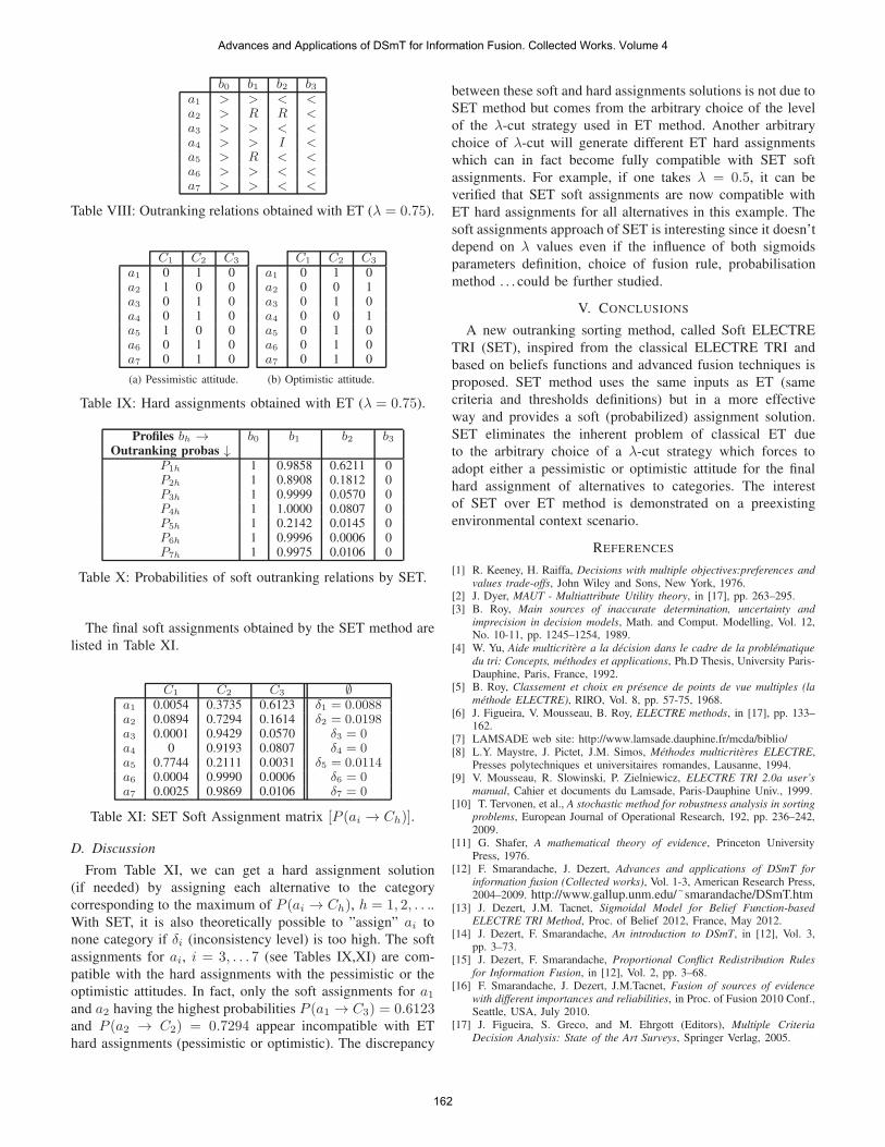
b0 b1 b2 b3a1 > > < <a2 > R R <a3 > > < <a4 > > I <a5 > R < <a6 > > < <a7 > > < <

Table VIII: Outranking relations obtained with ET (� = 0.75).

C1 C2 C3

a1 0 1 0a2 1 0 0a3 0 1 0a4 0 1 0a5 1 0 0a6 0 1 0a7 0 1 0

(a) Pessimistic attitude.

C1 C2 C3

a1 0 1 0a2 0 0 1a3 0 1 0a4 0 0 1a5 0 1 0a6 0 1 0a7 0 1 0

(b) Optimistic attitude.

Table IX: Hard assignments obtained with ET (� = 0.75).

Profiles bℎ → b0 b1 b2 b3Outranking probas ↓

P1ℎ 1 0.9858 0.6211 0P2ℎ 1 0.8908 0.1812 0P3ℎ 1 0.9999 0.0570 0P4ℎ 1 1.0000 0.0807 0P5ℎ 1 0.2142 0.0145 0P6ℎ 1 0.9996 0.0006 0P7ℎ 1 0.9975 0.0106 0

Table X: Probabilities of soft outranking relations by SET.

The final soft assignments obtained by the SET method are

listed in Table XI.

C1 C2 C3 ∅a1 0.0054 0.3735 0.6123 �1 = 0.0088a2 0.0894 0.7294 0.1614 �2 = 0.0198a3 0.0001 0.9429 0.0570 �3 = 0a4 0 0.9193 0.0807 �4 = 0a5 0.7744 0.2111 0.0031 �5 = 0.0114a6 0.0004 0.9990 0.0006 �6 = 0a7 0.0025 0.9869 0.0106 �7 = 0

Table XI: SET Soft Assignment matrix [P (ai → Cℎ)].

D. Discussion

From Table XI, we can get a hard assignment solution

(if needed) by assigning each alternative to the category

corresponding to the maximum of P (ai → Cℎ), ℎ = 1, 2, . . ..With SET, it is also theoretically possible to ”assign” ai to

none category if �i (inconsistency level) is too high. The soft

assignments for ai, i = 3, . . . 7 (see Tables IX,XI) are com-

patible with the hard assignments with the pessimistic or the

optimistic attitudes. In fact, only the soft assignments for a1and a2 having the highest probabilities P (a1 → C3) = 0.6123and P (a2 → C2) = 0.7294 appear incompatible with ET

hard assignments (pessimistic or optimistic). The discrepancy

between these soft and hard assignments solutions is not due to

SET method but comes from the arbitrary choice of the level

of the �-cut strategy used in ET method. Another arbitrary

choice of �-cut will generate different ET hard assignments

which can in fact become fully compatible with SET soft

assignments. For example, if one takes � = 0.5, it can be

verified that SET soft assignments are now compatible with

ET hard assignments for all alternatives in this example. The

soft assignments approach of SET is interesting since it doesn’t

depend on � values even if the influence of both sigmoids

parameters definition, choice of fusion rule, probabilisation

method . . . could be further studied.

V. CONCLUSIONS

A new outranking sorting method, called Soft ELECTRE

TRI (SET), inspired from the classical ELECTRE TRI and

based on beliefs functions and advanced fusion techniques is

proposed. SET method uses the same inputs as ET (same

criteria and thresholds definitions) but in a more effective

way and provides a soft (probabilized) assignment solution.

SET eliminates the inherent problem of classical ET due

to the arbitrary choice of a �-cut strategy which forces to

adopt either a pessimistic or optimistic attitude for the final

hard assignment of alternatives to categories. The interest

of SET over ET method is demonstrated on a preexisting

environmental context scenario.

REFERENCES

[1] R. Keeney, H. Raiffa, Decisions with multiple objectives:preferences and

values trade-offs, John Wiley and Sons, New York, 1976.[2] J. Dyer, MAUT - Multiattribute Utility theory, in [17], pp. 263–295.[3] B. Roy, Main sources of inaccurate determination, uncertainty and

imprecision in decision models, Math. and Comput. Modelling, Vol. 12,No. 10-11, pp. 1245–1254, 1989.

[4] W. Yu, Aide multicritere a la decision dans le cadre de la problematique

du tri: Concepts, methodes et applications, Ph.D Thesis, University Paris-Dauphine, Paris, France, 1992.

[5] B. Roy, Classement et choix en presence de points de vue multiples (la

methode ELECTRE), RIRO, Vol. 8, pp. 57-75, 1968.[6] J. Figueira, V. Mousseau, B. Roy, ELECTRE methods, in [17], pp. 133–

162.[7] LAMSADE web site: http://www.lamsade.dauphine.fr/mcda/biblio/[8] L.Y. Maystre, J. Pictet, J.M. Simos, Methodes multicriteres ELECTRE,

Presses polytechniques et universitaires romandes, Lausanne, 1994.[9] V. Mousseau, R. Slowinski, P. Zielniewicz, ELECTRE TRI 2.0a user’s

manual, Cahier et documents du Lamsade, Paris-Dauphine Univ., 1999.[10] T. Tervonen, et al., A stochastic method for robustness analysis in sorting

problems, European Journal of Operational Research, 192, pp. 236–242,2009.

[11] G. Shafer, A mathematical theory of evidence, Princeton UniversityPress, 1976.

[12] F. Smarandache, J. Dezert, Advances and applications of DSmT for

information fusion (Collected works), Vol. 1-3, American Research Press,2004–2009. http://www.gallup.unm.edu/˜smarandache/DSmT.htm

[13] J. Dezert, J.M. Tacnet, Sigmoidal Model for Belief Function-basedELECTRE TRI Method, Proc. of Belief 2012, France, May 2012.

[14] J. Dezert, F. Smarandache, An introduction to DSmT, in [12], Vol. 3,pp. 3–73.

[15] J. Dezert, F. Smarandache, Proportional Conflict Redistribution Rules

for Information Fusion, in [12], Vol. 2, pp. 3–68.[16] F. Smarandache, J. Dezert, J.M.Tacnet, Fusion of sources of evidence

with different importances and reliabilities, in Proc. of Fusion 2010 Conf.,Seattle, USA, July 2010.

[17] J. Figueira, S. Greco, and M. Ehrgott (Editors), Multiple Criteria

Decision Analysis: State of the Art Surveys, Springer Verlag, 2005.


162

Soft ELECTRE TRI Outranking Method Based on Belief Functions

Documents

Transcript of Soft ELECTRE TRI Outranking Method Based on Belief Functions