Soft Decoding of a Qubit Readout Apparatus

B. D’AnjouDepartment of Physics, McGill University, Montreal, Quebec, H3A 2T8, Canada

W.A. CoishDepartment of Physics, McGill University, Montreal, Quebec, H3A 2T8, Canada and

Canadian Institute for Advanced Research, Toronto, Ontario, M5G 1Z8, Canada(Dated: January 29, 2018)

Qubit readout is commonly performed by thresholding a collection of analog detector signals toobtain a sequence of single-shot bit values. The intrinsic irreversibility of the mapping from analogto digital signals discards soft information associated with an a posteriori confidence that can beassigned to each bit value when a detector is well characterized. Accounting for soft information,we show significant improvements in enhanced state detection with the quantum repetition code aswell as quantum state or parameter estimation. These advantages persist in spite of non-Gaussianfeatures of realistic readout models, experimentally relevant small numbers of qubits, and finiteencoding errors. These results show useful and achievable advantages for a wide range of currentexperiments on quantum state tomography, parameter estimation, and qubit readout.

PACS numbers: 03.65.Ta,03.67.Ac,03.65.Wj

In most quantum-measurement tasks, the goal is to ex-tract information encoded in a stream of quantum states.For a single-qubit expectation value, the stream is a col-lection of identically prepared single qubits. To performa Bell-inequality measurement, the stream is a collectionof entangled qubit pairs. For quantum error detectionor correction, the stream consists of many qubits thatmake up the code, on which multiqubit syndrome mea-surements are performed. In practice, in all of these sce-narios, information is commonly extracted by measuringindividual qubits or joint observables in a single shot [1–8]. While this strategy can be optimal for extractinga single bit of information, e.g., the state |±〉 of a sin-gle qubit, it is generally suboptimal when consideringstreams of data. A single-shot qubit readout typically in-volves the irreversible conversion of an analog outcome Ofrom a readout apparatus (e.g., a current or voltage pulse,the quadrature of a microwave tone, etc.) into a binaryoutcome c± via thresholding [9–17] (see Fig. 1). Thresh-olding erases information about the posterior probabilityP (±|O) that can be ascribed to each bit value given O.In contrast, when a sequence of analog readout outcomesO is fed into a decoder that accepts analog values as in-put, the frequency of decoding errors can be significantlyreduced [18]. Such soft-decoding techniques have beencentral to the development of capacity-achieving classicalcodes [19] now used in deep-space communications andhigh-bandwidth 3G/4G cellular networks. Soft-decisiondecoding has been applied to quantum codes [20, 21] andto schemes for fault-tolerant quantum computing [22], inwhich the soft decision is made by correlating multiplesingle-shot qubit readout outcomes. Soft decoding hasalso been identified as an important tool for continuous-variable quantum key distribution [23].

While soft-decoding methods are routinely applied to

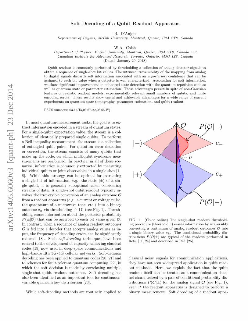
FIG. 1. (Color online) The single-shot readout threshold-ing procedure (threshold ν) erases information by irreversiblyconverting a continuum of analog readout outcomes O intoa single binary value c±. The conditional probability dis-tributions P (O|±) are typical of the readout performed inRefs. [11, 24] and described in Ref. [25].

classical noisy signals for communication applications,they have not seen widespread application in qubit read-out methods. Here, we exploit the fact that the qubitreadout itself can be treated as a communication chan-nel characterized by a pair of conditional probability dis-tributions P (O|±) for the analog signal O (see Fig. 1),even if the readout apparatus is designed to perform abinary measurement. Soft decoding of a readout appa-

arX

iv:1

405.

6060

v3 [

quan

t-ph

] 2

3 D

ec 2

014

2

ratus can lead to significant improvements in a numberof quantum-information tasks. To achieve these improve-ments, the physical characteristics of the readout dynam-ics and the noise must be well understood to determinethe distributions P (O|±). Readout errors are especiallysensitive to the tails of these distributions, so it is impor-tant to understand non-Gaussian features (fat tails orbimodality) to reap the benefits of soft decoding. Cru-cially, the distributions P (O|±), which must already beknown to characterize the single-shot readout fidelity, canbe measured or modeled accurately for several state-of-the-art qubit implementations [9–17, 25–28].

In this Letter, we explicitly demonstrate the advan-tages of soft decoding through two experimentally signif-icant examples: enhanced state detection via the quan-tum repetition code, and state or parameter estimation.In particular, the number of qubits required for efficientenhanced state detection can be reduced, through dataprocessing alone, by up to a factor of 2, an advantagewhich persists for a small number of qubits and finite en-coding errors. Because additional qubits are an expen-sive resource, this result is of immediate practical impor-tance. We also extend a result of Ref. [29] by makinguse of soft information to further improve the precisionof measurements of Pauli operators required for state to-mography. In both cases, we benchmark the improve-ment by comparing the performance of the widely usedand efficient maximum-likelihood estimation [30] whenapplied to analog instead of thresholded qubit readoutoutcomes. Crucially, we find and characterize signifi-cant improvements not only for the idealized Gaussianreadout, but also for the realistic non-Gaussian readoutinvestigated in Ref. [25] and relevant to many experi-ments [11, 14, 24, 26].

Enhanced state detection.− In the quantum repeti-tion code, a logical qubit (with basis {|0〉 , |1〉}) in thestate |ψ〉 = α0 |0〉 + α1 |1〉 is encoded into N physi-

cal qubits (with basis {|+〉 , |−〉}): |ψN 〉 = α0 |−〉⊗N +

α1 |+〉⊗N [31–33]. The redundant outcomes of indepen-dent measurements of the N physical qubits are thencorrelated to reduce measurement errors. The simplestapproach is to measure each qubit in a single shot andassign the binary value ci = c± to the ith qubit. Whenthe encoded states |0〉 and |1〉 are equally likely a pri-ori, the optimal approach is to calculate the likelihoodratio [34] of the data {ci}:

Λc ≡P ({ci} |1)

P ({ci} |0)=

N∏i=1

P (ci|+)

P (ci|−). (1)

In Eq. (1), P (ci|±) is the probability to obtain the valueci given that the ith qubit is in the state |±〉. The pro-jected state of the logical qubit is most likely |1〉 (|0〉) ifΛc > 1 (Λc < 1). We may rewrite the likelihood ratio,Eq. (1), in terms of the conditional single-shot error rates

ε± ≡ P (c∓|±) < 1/2:

Λc =

(1− ε+ε−

)n+

·(

ε+1− ε−

)N−n+

, (2)

where n+ is the number of measurements for which theoutcome c+ occurred. For a binary symmetric readout,ε = ε±, Eq. (2) results in a simple majority vote sincen+ > N/2 (n+ < N/2) implies Λc > 1 (Λc < 1).

Equation (2) is a maximum-likelihood estimator ap-plied to single-shot readout outcomes. However, a physi-cal readout apparatus typically yields an analog readoutoutcome Oi that need not be thresholded to a binaryvalue ci. The observable Oi could be, for example, thetime average of a fluorescence signal [9, 13, 33], the peakof a current pulse through a single-electron transistor orquantum point contact [11, 24, 26], the quadrature of amicrowave tone [15, 16, 27], or even the likelihood ratioof a single-shot readout [9, 17, 25, 28, 35]. Thresholdingleads to an irreversible loss of information about the con-fidence P (±|Oi) in each bit value. Soft decoding, whichmakes full use of that information, is achieved by insteadapplying the maximum-likelihood estimator to the ana-log readout outcomes:

ΛO ≡P ({Oi} |1)

P ({Oi} |0)=

N∏i=1

P (Oi|+)

P (Oi|−), (3)

where P (Oi|±) is the probability density for outcome Oigiven that the ith qubit is in the state |±〉.

To take full advantage of soft decoding, it is nec-essary to have an accurate representation of the con-ditional probability distributions P (O|±) for the ana-log qubit readout outcomes. A common idealizationfor a readout is the Gaussian readout, P (O|±) =√r/2π exp

[−(O ∓ 1)2r/2

], where r is the power signal-

to-noise ratio. Soft decoding of the Gaussian readoutwith maximum-likelihood estimators such as Eqs. (1) and(3) has been extensively studied in the context of clas-sical communication theory [18, 34]. Since a projective

measurement collapses |ψN 〉 to either |+〉⊗N or |−〉⊗N ,the advantage obtained by soft decoding of the readoutapparatus translates directly to the quantum case. Moreprecisely, for r � 1, the number of qubits Nc and NO re-quired to achieve a target error rate ε using Λc and ΛO,respectively, are related (for Nc odd) by [36]:

NO =Nc + 1

2+Nc − 1

2

ln r

r+O

(Ncr

). (4)

Thus, soft decoding can reduce the number of requiredphysical qubits by up to a factor of 2 compared to themajority vote (asymptotically, Nc ∼ 2NO, or alterna-tively, for fixed N , εO ∼ ε2c up to a logarithmic prefactorin εc). Intuitively, this advantage arises since the major-ity vote ignores all information contained in strings forwhich more than half of the bits are corrupted, while

3

soft decoding associates every string with some confi-dence. A similar asymptotic advantage exists for arbi-trary block codes transmitted through a Gaussian com-munication channel [18]. Importantly, Eq. (4) is validfor the regime of reasonably small N relevant to recentexperiments [2, 5–8, 37, 38]. Moreover, the form of thesubleading corrections in Eq. (4) suggests that they canbe small for realistic experimental values of r. We haveindeed verified, using the exact analytical expressions forthe error rates [36], that an advantage persists for lowsignal-to-noise ratio and relatively small N . For exam-ple, we require NO = 6 instead of Nc = 9 to reach anerror rate ε < 3× 10−4 for r = 2.

Realistic qubit readouts are typically not well repre-sented by Gaussian probability distributions [9, 11, 13,25, 28]. To verify that soft decoding of the readout ap-paratus still provides an advantage in experimentally rel-evant cases, we apply the estimators in Eqs. (1) and (3)to the realistic non-Gaussian “peak-signal” readout im-plemented in Refs. [11, 24] and for which the distribu-tions P (O|±) were analyzed in Ref. [25]. In this mea-surement, the analog outcome O is the peak value of afinite-duration current pulse signalling the excited state|+〉 and subject to Gaussian white noise (see Ref. [36]for a summary). A typical pair of distributions for thisreadout is illustrated in Fig. 1. Even though the dis-tribution P (O|+) has strong non-Gaussian features, softdecoding still gives an appreciable advantage. For exam-ple, Monte Carlo simulations with 106 random recordsshow that, similar to the Gaussian readout, we requireNO = 6 instead of Nc = 9 to reach an error rate ε < 0.05for a signal-to-noise ratio r = 2 [36].

To account for errors during encoding, we allow foruncorrelated bit flips with probability η for both states|±〉. The probability distributions for the analog read-out outcomes then become P (Oi|1/0) = (1 − η)P (Oi| +/−)+ηP (Oi|−/+), giving a modified version of the like-lihood ratio, Eq. (3). We find that when encoding errorsη are sufficiently large, the soft-decoding procedure re-duces to a simple thresholding procedure [36]. However,for the Gaussian readout, soft decoding can still give anadvantage over thresholding if

η . e−2r (5)

when r � 1. Thus, the encoding bit-flip rate must merelybe smaller than some power of the single-shot readouterror rate ε (ε ∼ e−

r2 up to logarithmic corrections). To

verify this, we have performed a Monte Carlo simulationof the error rate for the Gaussian readout by generating107 random measurement records taking into account thebit-flip rate η [36]. For example, we find that for r = 2and η = 1%, we require NO = 6 instead of Nc = 9 qubitsto achieve ε < 8 × 10−4. Similarly, for the peak-signalreadout described in Ref. [25], we find from a simulationof 106 random measurement records that for a signal-to-noise ratio of r = 2 and η = 5%, we require NO = 6

instead of Nc = 9 qubits to achieve ε < 0.08 [36].

State and parameter estimation.− Many quantum in-formation processing applications, such as state and pro-cess tomography [1, 4, 29, 39, 40] and parameter estima-tion [41], benefit from accurate and precise estimationof qubit observables (e.g., the Pauli operators). Analogdata processing has been used extensively, e.g., for pa-rameter [42] and state [43] estimation in quantum opticalsystems, where it is often natural to process quasicontinu-ous field quadratures or photon counts. For many qubitsystems, the common approach is instead to thresholdthe data. Thresholding the data is generally suboptimal,as we now illustrate.

For definiteness, we consider estimating the quantumexpectation value s0 = 〈σz〉 of the single-qubit Pauli op-erator σz (in the basis |±〉) from the independent read-out of N identically prepared copies of a qubit. As inthe case of the repetition code, we compare the stan-dard maximum-likelihood estimator (MLE) [30] appliedto the analog data set {Oi} instead of the thresholdeddata set {ci} in order to benchmark the improvement.In both cases, the MLE is the value s that maximizesthe likelihood function L(s) =

∏Ni=1 P (Oi/ci|s) under

the constraint −1 ≤ s ≤ +1. In practice, the MLEis obtained by maximizing the equivalent log-likelihoodfunction `(s) = N−1 lnL(s). The MLE is asymptoticallyunbiased, normally distributed, and minimizes the vari-ance [i.e. saturates the Cramer-Rao bound, see Eq. (7),below] for large N [30].

When the analog data are thresholded, the MLE is the(bias-corrected) thresholded average sTA = N−1

∑Ni=1 ci

considered, e.g., in Ref. [29]. This estimate does not makeuse of the soft information contained in the distributionsP (O|±) for reconstruction of s0. In contrast, the soft-decoded estimate sSD obtained by applying the MLE tothe analog data set makes full use of the distributionsP (O|±). In Ref. [29], the alternative soft average sSA =

N−1∑Ni=1Oi was also employed as an estimator for s0,

but this approach is also suboptimal [36].

We will measure the deviation of an estimate s fromthe true value s0 with the mean squared error (MSE) ζ,given by the sum of the variance and of the squared biasof the estimator, ζ ≡

⟨⟨(s− 〈〈s〉〉)2

⟩⟩+ (〈〈s〉〉− s0)2. Here,

the statistical average 〈〈 〉〉 is taken with respect to thedistribution of outcomes:

P (O/c|s0) =1 + s0

2P (O/c|+) +

1− s02

P (O/c|−). (6)

For this distribution, `(s) is a concave function with aunique maximum. A general expression for the asymp-totic MSE of the thresholded average sTA can be de-rived [36]. For the Gaussian readout, it takes the simple

form reported in Ref. [29], ζTA ∼ [(1− 2ε)−2 − s20]/N .

For the soft-decoded MLE estimate, the asymptotic MSEcan be computed directly from the Fisher information of

4

P (O|s0):

ζSD ∼ −1

N

⟨⟨∂2 lnP (O|s0)

∂s20

⟩⟩−1. (7)

Here, we use the symbol “∼” to indicate a strict asymp-totic equality. From Eqs. (6) and (7), an explicit asymp-totic form for ζSD can be found in terms of the distribu-tions P (O|±) [36]:

ζSD ∼1

N· 1− s20

1− I, I =

∫dO P (O|+)P (O|−)

P (O|s0). (8)

In Eq. (8), the integral I contains all information aboutthe noise introduced by the readout apparatus. The re-maining contribution when I = 0 is the quantum shotnoise (projection noise), which reflects the choice of aparticular measurement basis. Since I has the form ofan overlap integral, it is especially important to under-stand the tails of the (generally non-Gaussian) readoutdistributions P (O|±).

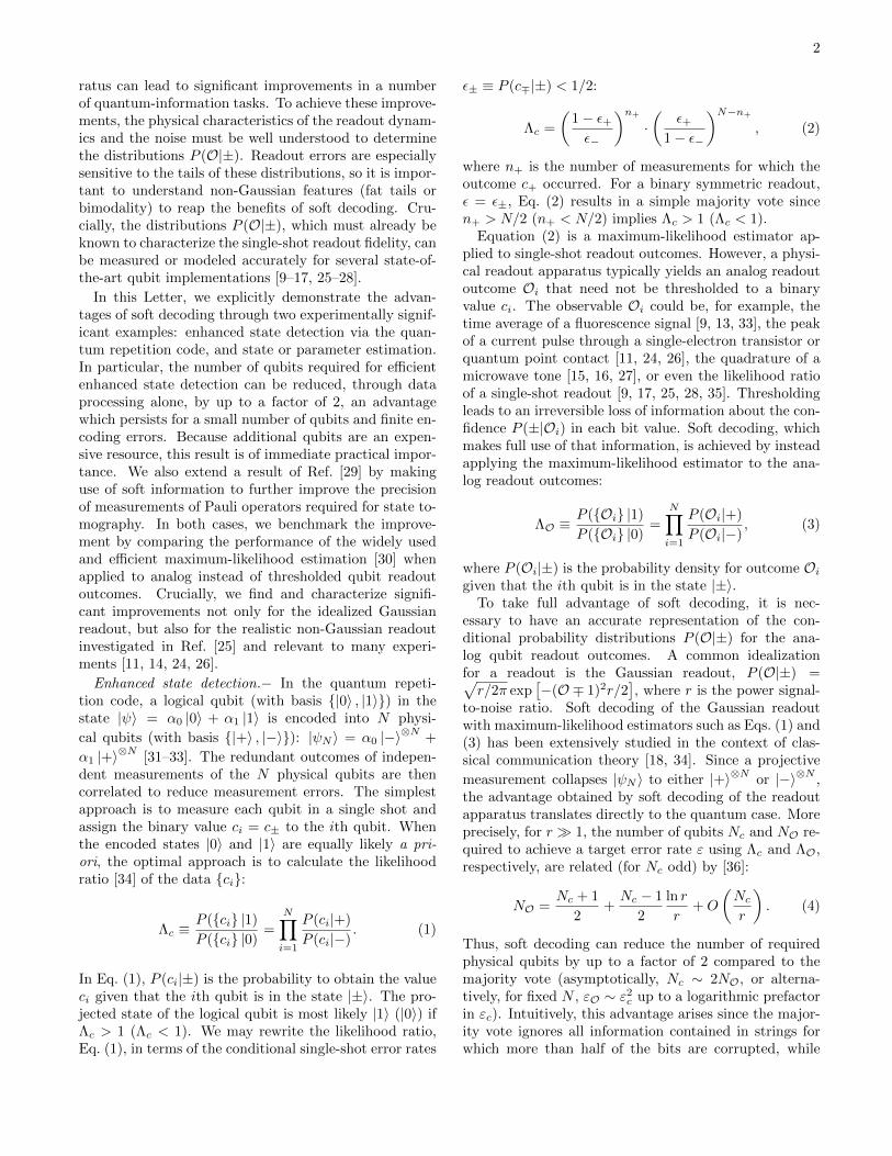
To quantitatively verify that soft decoding can im-prove state estimation, we set s0 = 0 and evaluateEq. (8) numerically for both the Gaussian readout andthe peak-signal readout of Ref. [25]. We plot the asymp-totic MSE as a function of the signal-to-noise ratio rin Fig. 2. We also plot the asymptotic MSE of thebias-corrected thresholded average, ζTA. Figure 2 con-firms that soft decoding always outperforms threshold-ing (i.e., ζSD < ζTA). As r increases, ζTA and ζSD exhibitan approximate power-law approach to the projection-noise limit for the (non-Gaussian) peak-signal readoutof Ref. [25], whereas they decrease exponentially for theGaussian readout. In the intermediate regime for r, thereis a clear advantage in soft decoding with the MLE forboth readouts, demonstrating substantial benefits in theexperimentally relevant regime of signal-to-noise ratios,r ∼ 1 for the Gaussian readout [29], and r ∼ 10 for thepeak-signal readout.

To show that the asymptotic advantage persists whenN is finite, we calculate ζ from a Monte Carlo sim-ulation with N = 100. We first randomly generate5 × 104 measurement records {Oi} from the distribu-

tion∏Ni=1 P (Oi|s0) for both the Gaussian readout and

non-Gaussian peak-signal readout of Ref. [25]. For eachmeasurement record, we calculate sTA and optimize thelog-likelihood function `(s) to obtain sSD. We then di-rectly obtain ζ from the variance and bias of the simu-lated estimates. The results are displayed (open symbols)in Fig. 2 for s0 = 0. The simulated data points coincidewith the asymptotic predictions.

In conclusion, we have shown that making use of thesoft information contained in the analog outcomes ofa qubit readout apparatus, as opposed to irreversiblythresholding each qubit to a binary value, can signif-icantly improve the performance of quantum informa-tion processing tasks involving the measurement of many

FIG. 2. (Color online) Asymptotic normalized MSEs N · ζof the soft-decoded estimate (solid gold), Eq. (8), and ofthe thresholded average (dot-dashed magenta line), given inRef. [36], as a function of the signal-to-noise ratio r assum-ing s0 = 〈σz〉 = 0 for (a) the Gaussian readout and (b) the“peak-signal” readout of Ref. [25]. The finite-N MSEs of thethresholded average (magenta squares) and soft-decoded es-timate (gold triangles) are obtained from 5 × 104 randomlygenerated measurement records of N = 100 qubits. Insets:Asymptotic MSEs on a logarithmic scale.

qubits. We have focused on two examples of practical im-portance. In the case of enhanced state detection withthe quantum repetition code, the number of qubits re-quired to achieve a given error rate can be reduced byup to a factor of 2 through improved data processingalone. Importantly, we have shown that an advantagepersists for small numbers of qubits and finite encodingerrors. In addition, we have shown that optimal process-ing of analog qubit readout outcomes can appreciablyincrease the precision on the measurement of qubit ob-servables (e.g., the Pauli operators). Crucially, in bothcases we have demonstrated a significant improvementfor an experimentally relevant, non-Gaussian qubit read-out model [11, 14, 24–26].

Our results offer encouraging prospects for direct im-provements of both small and large scale quantum infor-mation processing applications through soft decoding of

5

the qubit readout. For example, readout error models fordecoders of topological codes [21, 44] could be modifiedusing the ideas presented here to accept analog readoutoutcomes with realistic statistics at the single-physical-qubit level, improving error detection rates. While thereare many possible extensions of this work, the directimprovements we have shown to enhanced state detec-tion and quantum state or parameter estimation are bothpractical and immediately realizable in a wide array ofcurrent experiments.

We thank L. Childress, A. Fowler, and D. Poulin foruseful discussions. We acknowledge financial supportfrom the National Sciences and Engineering ResearchCouncil of Canada (NSERC), the Canadian Institute forAdvanced Research (CIFAR), the Fonds the Recherchedu Quebec Nature et Technologies (FRQNT), and theInstitut Transdisciplinaire d’Information Quantique (IN-TRIQ).

[1] H. Haffner, W. Hansel, C. Roos, J. Benhelm, M. Chwalla,T. Korber, U. Rapol, M. Riebe, P. Schmidt, C. Becher,et al., Nature 438, 643 (2005).

[2] P. Schindler, J. T. Barreiro, T. Monz, V. Nebendahl,D. Nigg, M. Chwalla, M. Hennrich, and R. Blatt, Science332, 1059 (2011).

[3] H. Bernien, B. Hensen, W. Pfaff, G. Koolstra, M. Blok,L. Robledo, T. Taminiau, M. Markham, D. Twitchen,L. Childress, et al., Nature 497, 86 (2013).

[4] J. M. Chow, A. D. Corcoles, J. M. Gambetta, C. Rigetti,B. R. Johnson, J. A. Smolin, J. R. Rozen, G. A. Keefe,M. B. Rothwell, M. B. Ketchen, and M. Steffen, Phys.Rev. Lett. 107, 080502 (2011).

[5] M. Reed, L. DiCarlo, S. Nigg, L. Sun, L. Frunzio,S. Girvin, and R. Schoelkopf, Nature 482, 382 (2012).

[6] J. M. Chow, J. M. Gambetta, E. Magesan, S. J. Srini-vasan, A. W. Cross, D. W. Abraham, N. A. Masluk,B. Johnson, C. A. Ryan, and M. Steffen, arXiv:1311.6330(2013).

[7] O.-P. Saira, J. P. Groen, J. Cramer, M. Meretska,G. de Lange, and L. DiCarlo, Phys. Rev. Lett. 112,070502 (2014).

[8] R. Barends, J. Kelly, A. Megrant, A. Veitia, D. Sank,E. Jeffrey, T. White, J. Mutus, A. Fowler, B. Campbell,et al., Nature 508, 500 (2014).

[9] A. H. Myerson, D. J. Szwer, S. C. Webster, D. T. C.Allcock, M. J. Curtis, G. Imreh, J. A. Sherman, D. N.Stacey, A. M. Steane, and D. M. Lucas, Phys. Rev. Lett.100, 200502 (2008).

[10] C. Barthel, D. J. Reilly, C. M. Marcus, M. P. Hanson,and A. C. Gossard, Phys. Rev. Lett. 103, 160503 (2009).

[11] A. Morello, J. J. Pla, F. A. Zwanenburg, K. W. Chan,K. Y. Tan, H. Huebl, M. Mottonen, C. D. Nugroho,C. Yang, J. A. van Donkelaar, et al., Nature 467, 687(2010).

[12] P. Neumann, J. Beck, M. Steiner, F. Rempp, H. Fedder,P. R. Hemmer, J. Wrachtrup, and F. Jelezko, Science329, 542 (2010).

[13] L. Robledo, L. Childress, H. Bernien, B. Hensen, P. F.

Alkemade, and R. Hanson, Nature 477, 574 (2011).[14] J. J. Pla, K. Y. Tan, J. P. Dehollain, W. H. Lim, J. J.

Morton, F. A. Zwanenburg, D. N. Jamieson, A. S. Dzu-rak, and A. Morello, Nature 496, 334 (2013).

[15] Z. R. Lin, K. Inomata, W. D. Oliver, K. Koshino,Y. Nakamura, J. S. Tsai, and T. Yamamoto, Appl. Phys.Lett. 103, 132602 (2013).

[16] Y. Liu, S. Srinivasan, D. Hover, S. Zhu, R. McDermott,and A. Houck, arXiv:1401.5184 (2014).

[17] T. Harty, D. Allcock, C. Ballance, L. Guidoni,H. Janacek, N. Linke, D. Stacey, and D. Lucas,arXiv:1403.1524 (2014).

[18] D. Chase, Information Theory, IEEE Transactions on 18,170 (1972).

[19] E. Guizzo, “Closing in on the perfect code,”http://spectrum.ieee.org/computing/software/closing-in-on-the-perfect-code (2004).

[20] D. Poulin, Phys. Rev. A 74, 052333 (2006).[21] G. Duclos-Cianci and D. Poulin, in Information Theory

Workshop (ITW), 2010 IEEE (IEEE, 2010) pp. 1–5.[22] H. Goto and H. Uchikawa, Scientific reports 3 (2013).[23] M. Mondin, F. Daneshgaran, M. Delgado, and F. Mesiti,

in Personal Satellite Services (Springer, 2010) pp. 305–316.

[24] J. M. Elzerman, R. Hanson, L. H. W. Van Beveren,B. Witkamp, L. M. K. Vandersypen, and L. P. Kouwen-hoven, Nature 430, 431 (2004).

[25] B. D’Anjou and W. A. Coish, Phys. Rev. A 89, 012313(2014).

[26] M. Veldhorst, J. C. C. Hwang, C. H. Yang, A. W. Leen-stra, B. de Ronde, J. P. Dehollain, J. T. Muhonen, F. E.Hudson, K. M. Itoh, A. Morello, and A. S. Dzurak, arXivpreprint arXiv:1407.1950 (2014).

[27] E. Jeffrey, D. Sank, J. Y. Mutus, T. C. White, J. Kelly,R. Barends, Y. Chen, Z. Chen, B. Chiaro, A. Dunsworth,A. Megrant, P. J. J. O’Malley, C. Neill, P. Roushan,A. Vainsencher, J. Wenner, A. N. Cleland, and J. M.Martinis, Phys. Rev. Lett. 112, 190504 (2014).

[28] J. Gambetta, W. A. Braff, A. Wallraff, S. M. Girvin, andR. J. Schoelkopf, Phys. Rev. A 76, 012325 (2007).

[29] C. A. Ryan, B. R. Johnson, J. M. Gambetta, J. M.Chow, M. P. da Silva, O. E. Dial, and T. A. Ohki,arXiv:1310.6448 (2013).

[30] H. Cramer, Mathematical methods of statistics (Prince-ton University Press, Princeton, NJ, 1946) Chap. 32-33.

[31] P. Deuar and W. J. Munro, Phys. Rev. A 61, 010306(1999).

[32] D. P. DiVincenzo, in Scalable Quantum Computers:Paving the Way to Realization, edited by S. L. Braun-stein, H.-K. Lo, and P. Kok (Wiley-VCH, Berlin, Ger-many, 2001) Chap. 1, pp. 1–13.

[33] T. Schaetz, M. D. Barrett, D. Leibfried, J. Britton,J. Chiaverini, W. M. Itano, J. D. Jost, E. Knill,C. Langer, and D. J. Wineland, Phys. Rev. Lett. 94,010501 (2005).

[34] J. M. Wozencraft and I. M. Jacobs, Principles of com-munication engineering (John Wiley & Sons, New York,U.S.A., 1965) Chap. 4.

[35] D. B. Hume, T. Rosenband, and D. J. Wineland, Phys.Rev. Lett. 99, 120502 (2007).

[36] “See Supplemental Material at [...], which includes detailson derivations and Monte Carlo simulations as well asRefs. [45, 46],”.

[37] T. Monz, P. Schindler, J. T. Barreiro, M. Chwalla,

6

D. Nigg, W. A. Coish, M. Harlander, W. Hansel, M. Hen-nrich, and R. Blatt, Phys. Rev. Lett. 106, 130506 (2011).

[38] J. F. Goodwin, B. J. Brown, G. Stutter, H. Dale, R. C.Thompson, and T. Rudolph, arXiv:1407.1858 (2014).

[39] S. T. Merkel, J. M. Gambetta, J. A. Smolin, S. Poletto,A. D. Corcoles, B. R. Johnson, C. A. Ryan, and M. Stef-fen, Phys. Rev. A 87, 062119 (2013).

[40] J. Medford, J. Beil, J. M. Taylor, S. D. Bartlett, A. C.Doherty, E. I. Rashba, D. P. DiVincenzo, H. Lu, A. C.Gossard, and C. M. Marcus, Nat. Nanotechnol. 8, 654(2013).

[41] M. D. Shulman, S. P. Harvey, J. M. Nichol, S. D.Bartlett, A. C. Doherty, V. Umansky, and A. Yacoby,arXiv:1405.0485 (2014).

[42] H. M. Wiseman and R. B. Killip, Phys. Rev. A 56, 944(1997).

[43] K. Banaszek, G. M. D’Ariano, M. G. A. Paris, and M. F.Sacchi, Phys. Rev. A 61, 010304 (1999).

[44] A. G. Fowler, A. C. Whiteside, A. L. McInnes, andA. Rabbani, Phys. Rev. X 2, 041003 (2012).

[45] R. Y. Rubinstein and D. P. Kroese, Simulation and theMonte Carlo method, 2nd ed. (John Wiley & Sons, Hobo-ken, U.S.A., 2008) Chap. 2, pp. 51–54.

[46] W. Press, B. Flannery, S. Teukolsky, and W. Vetterling,Numerical Recipes in Fortran 77: the art of scientificcomputing, 2nd ed. (Cambridge University Press, Cam-bridge, United Kingdom, 1992) Chap. 6, pp. 219–222.

7

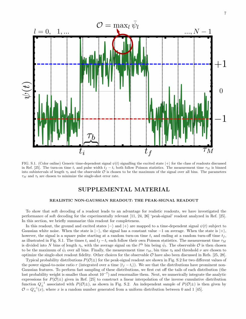
FIG. S.1. (Color online) Generic time-dependent signal ψ(t) signalling the excited state |+〉 for the class of readouts discussedin Ref. [25]. The turn-on time ti and pulse width tf − ti both follow Poisson statistics. The measurement time τM is binnedinto subintervals of length τb and the observable O is chosen to be the maximum of the signal over all bins. The parametersτM and τb are chosen to minimize the single-shot error rate.

SUPPLEMENTAL MATERIAL

REALISTIC NON-GAUSSIAN READOUT: THE PEAK-SIGNAL READOUT

To show that soft decoding of a readout leads to an advantage for realistic readouts, we have investigated theperformance of soft decoding for the experimentally relevant [11, 24, 26] ‘peak-signal’ readout analyzed in Ref. [25].In this section, we briefly summarize this readout for completeness.

In this readout, the ground and excited states |−〉 and |+〉 are mapped to a time-dependent signal ψ(t) subject toGaussian white noise. When the state is |−〉, the signal has a constant value −1 on average. When the state is |+〉,however, the signal is a square pulse starting at a random turn-on time ti and ending at a random turn-off time tf ,as illustrated in Fig. S.1. The times ti and tf − ti each follow their own Poisson statistics. The measurement time τMis divided into N bins of length τb, with the average signal on the lth bin being ψl. The observable O is then chosento be the maximum of ψl over all bins. Finally, the measurement time τM , bin time τb and threshold ν are chosen tooptimize the single-shot readout fidelity. Other choices for the observable O have also been discussed in Refs. [25, 28].

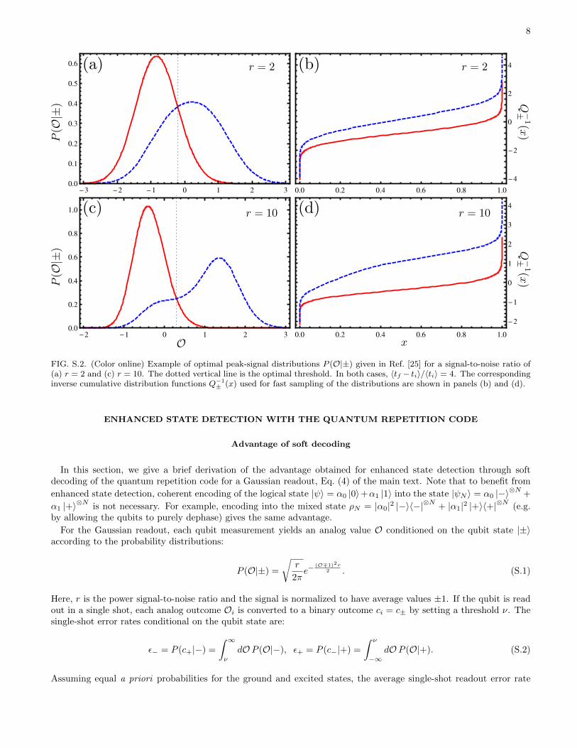
Typical probability distributions P (O|±) for the peak-signal readout are shown in Fig. S.2 for two different values ofthe power signal-to-noise ratio r (integrated over a time 〈tf − ti〉). We see that the distributions have prominent non-Gaussian features. To perform fast sampling of these distributions, we first cut off the tails of each distribution (thelost probability weight is smaller than about 10−7) and renormalize them. Next, we numerically integrate the analyticexpressions for P (O|±) given in Ref. [25] to construct a linear interpolation of the inverse cumulative distributionfunction Q−1± associated with P (O|±), as shown in Fig. S.2. An independent sample of P (O|±) is then given by

O = Q−1± (x), where x is a random number generated from a uniform distribution between 0 and 1 [45].

8

FIG. S.2. (Color online) Example of optimal peak-signal distributions P (O|±) given in Ref. [25] for a signal-to-noise ratio of(a) r = 2 and (c) r = 10. The dotted vertical line is the optimal threshold. In both cases, 〈tf − ti〉/〈ti〉 = 4. The correspondinginverse cumulative distribution functions Q−1

± (x) used for fast sampling of the distributions are shown in panels (b) and (d).

ENHANCED STATE DETECTION WITH THE QUANTUM REPETITION CODE

Advantage of soft decoding

In this section, we give a brief derivation of the advantage obtained for enhanced state detection through softdecoding of the quantum repetition code for a Gaussian readout, Eq. (4) of the main text. Note that to benefit from

enhanced state detection, coherent encoding of the logical state |ψ〉 = α0 |0〉+α1 |1〉 into the state |ψN 〉 = α0 |−〉⊗N +

α1 |+〉⊗N is not necessary. For example, encoding into the mixed state ρN = |α0|2 |−〉〈−|⊗N + |α1|2 |+〉〈+|⊗N (e.g.by allowing the qubits to purely dephase) gives the same advantage.

For the Gaussian readout, each qubit measurement yields an analog value O conditioned on the qubit state |±〉according to the probability distributions:

P (O|±) =

√r

2πe−

(O∓1)2r2 . (S.1)

Here, r is the power signal-to-noise ratio and the signal is normalized to have average values ±1. If the qubit is readout in a single shot, each analog outcome Oi is converted to a binary outcome ci = c± by setting a threshold ν. Thesingle-shot error rates conditional on the qubit state are:

ε− = P (c+|−) =

∫ ∞ν

dO P (O|−), ε+ = P (c−|+) =

∫ ν

−∞dO P (O|+). (S.2)

Assuming equal a priori probabilities for the ground and excited states, the average single-shot readout error rate

9

ε = (ε+ + ε−)/2 is minimized by choosing P (ν|+) = P (ν|−)⇒ ν = 0. An explicit calculation of the integrals gives:

ε = ε± =1

2erfc

(√r

2

). (S.3)

Eq. (S.3) defines the binary symmetric readout associated with the Gaussian readout.

We assume for simplicity that when the N qubits of the quantum repetition code are measured, the N -qubits statecollapses to |+〉⊗N or |−〉⊗N with equal probability. The resulting dataset consists of N analog readout outcomes Oi.In the main text, we gave two likelihood ratios Λc and ΛO for thresholded and analog readout outcomes, respectively.In both cases, if Λ > 1 (Λ < 1) we infer that the qubit state is |1〉 (|0〉). For the Gaussian readout, the likelihoodratios reduce to:

Λc =

(1− εε

)2n+−N

, ΛO = exp(2NrO

), (S.4)

where n+ is the number of times that the outcome Oi is converted to c+ if the qubits are read out in a single shot

and where O = N−1∑Ni=1Oi is the sample average of the analog outcomes [7].

Since ε < 1/2, the likelihood ratio Λc is equivalent to majority vote decoding of the repetition code. The corre-sponding average error rate εc is given by the probability that n+ > N/2 given that |0〉 is encoded, which is the sameas the probability that n+ < N/2 given that |1〉 is encoded. If N = 2M − 1 is odd, εc is given by:

εc =

N∑n+=N+1

2

(N

n+

)εn+(1− ε)N−n+ = Iε

(N + 1

2,N + 1

2

). (S.5)

Here, Iε(a, b) is the regularized incomplete beta function [46]. The error rate for N = 2M is the same since the casen+ = N/2 provides no information on the qubit state for a binary symmetric readout. For r large enough (Nε� 1),Eq. (S.5) takes the approximate form:

εc '(NN+12

)1

(2πr)N+1

4

e−(N+1)r

4 . (S.6)

Eq. (S.6) must be contrasted to the error rate for the likelihood ratio ΛO in Eq. (S.4). The corresponding averageerror rate εO is given by the probability that O > 0 given that |0〉 is encoded, which is the same as the probabilitythat O < 0 given that |1〉 is encoded. Since P (O|1) and P (O|0) are also Gaussians centered at ±1 with signal-to-noiseratio Nr, the average error rate for the soft decoding of the readout apparatus is simply:

εO =

∫ ∞0

dO P (O|0) =1

2erfc

(√Nr

2

). (S.7)

When r � 1, Eq. (S.7) becomes:

εO '1√

2πNre−

Nr2 . (S.8)

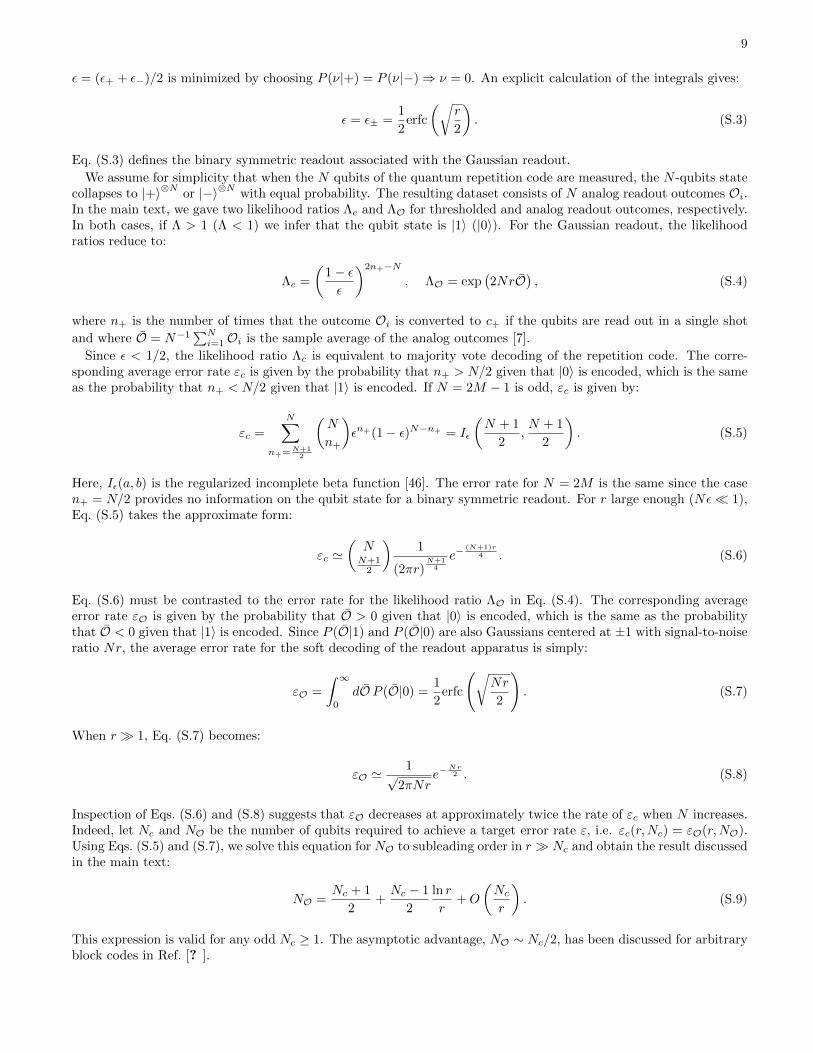
Inspection of Eqs. (S.6) and (S.8) suggests that εO decreases at approximately twice the rate of εc when N increases.Indeed, let Nc and NO be the number of qubits required to achieve a target error rate ε, i.e. εc(r,Nc) = εO(r,NO).Using Eqs. (S.5) and (S.7), we solve this equation for NO to subleading order in r � Nc and obtain the result discussedin the main text:

NO =Nc + 1

2+Nc − 1

2

ln r

r+O

(Ncr

). (S.9)

This expression is valid for any odd Nc ≥ 1. The asymptotic advantage, NO ∼ Nc/2, has been discussed for arbitraryblock codes in Ref. [? ].

10

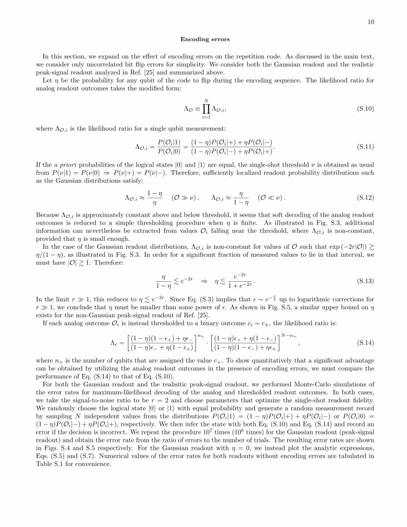
Encoding errors

In this section, we expand on the effect of encoding errors on the repetition code. As discussed in the main text,we consider only uncorrelated bit flip errors for simplicity. We consider both the Gaussian readout and the realisticpeak-signal readout analyzed in Ref. [25] and summarized above.

Let η be the probability for any qubit of the code to flip during the encoding sequence. The likelihood ratio foranalog readout outcomes takes the modified form:

ΛO ≡N∏i=1

ΛO,i, (S.10)

where ΛO,i is the likelihood ratio for a single qubit measurement:

ΛO,i =P (Oi|1)

P (Oi|0)=

(1− η)P (Oi|+) + ηP (Oi|−)

(1− η)P (Oi|−) + ηP (Oi|+). (S.11)

If the a priori probabilities of the logical states |0〉 and |1〉 are equal, the single-shot threshold ν is obtained as usualfrom P (ν|1) = P (ν|0) ⇒ P (ν|+) = P (ν|−). Therefore, sufficiently localized readout probability distributions suchas the Gaussian distributions satisfy:

ΛO,i ≈1− ηη

(O � ν) , ΛO,i ≈η

1− η(O � ν) . (S.12)

Because ΛO,i is approximately constant above and below threshold, it seems that soft decoding of the analog readoutoutcomes is reduced to a simple thresholding procedure when η is finite. As illustrated in Fig. S.3, additionalinformation can nevertheless be extracted from values Oi falling near the threshold, where ΛO,i is non-constant,provided that η is small enough.

In the case of the Gaussian readout distributions, ΛO,i is non-constant for values of O such that exp (−2r|O|) &η/(1 − η), as illustrated in Fig. S.3. In order for a significant fraction of measured values to lie in that interval, wemust have |O| & 1. Therefore:

η

1− η. e−2r ⇒ η .

e−2r

1 + e−2r. (S.13)

In the limit r � 1, this reduces to η . e−2r. Since Eq. (S.3) implies that ε ∼ e−r2 up to logarithmic corrections for

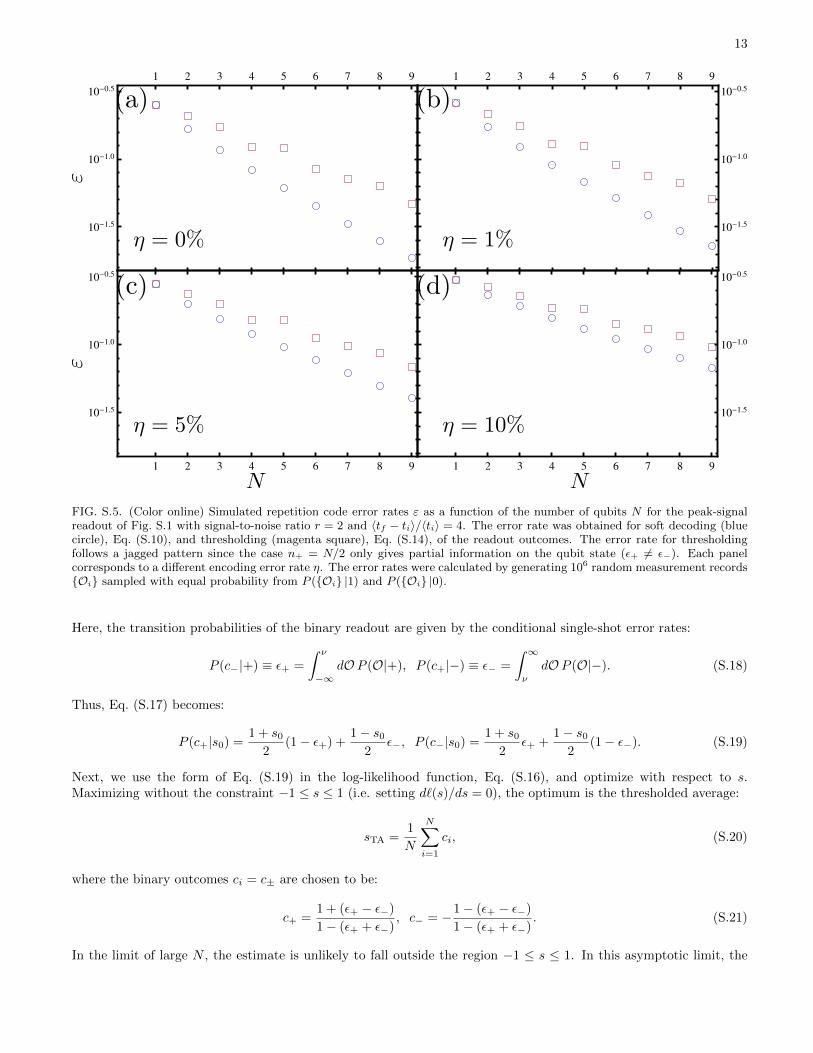
r � 1, we conclude that η must be smaller than some power of ε. As shown in Fig. S.5, a similar upper bound on ηexists for the non-Gaussian peak-signal readout of Ref. [25].

If each analog outcome Oi is instead thresholded to a binary outcome ci = c±, the likelihood ratio is:

Λc =

[(1− η)(1− ε+) + ηε−(1− η)ε− + η(1− ε+)

]n+

·[

(1− η)ε+ + η(1− ε−)

(1− η)(1− ε−) + ηε+

]N−n+

, (S.14)

where n+ is the number of qubits that are assigned the value c+. To show quantitatively that a significant advantagecan be obtained by utilizing the analog readout outcomes in the presence of encoding errors, we must compare theperformance of Eq. (S.14) to that of Eq. (S.10).

For both the Gaussian readout and the realisitic peak-signal readout, we performed Monte-Carlo simulations ofthe error rates for maximum-likelihood decoding of the analog and thresholded readout outcomes. In both cases,we take the signal-to-noise ratio to be r = 2 and choose parameters that optimize the single-shot readout fidelity.We randomly choose the logical state |0〉 or |1〉 with equal probability and generate a random measurement recordby sampling N independent values from the distributions P (Oi|1) = (1 − η)P (Oi|+) + ηP (Oi|−) or P (Oi|0) =(1− η)P (Oi|−) + ηP (Oi|+), respectively. We then infer the state with both Eq. (S.10) and Eq. (S.14) and record anerror if the decision is incorrect. We repeat the procedure 107 times (106 times) for the Gaussian readout (peak-signalreadout) and obtain the error rate from the ratio of errors to the number of trials. The resulting error rates are shownin Figs. S.4 and S.5 respectively. For the Gaussian readout with η = 0, we instead plot the analytic expressions,Eqs. (S.5) and (S.7). Numerical values of the error rates for both readouts without encoding errors are tabulated inTable S.1 for convenience.

11

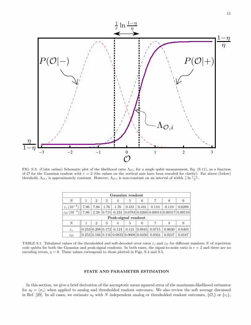
FIG. S.3. (Color online) Schematic plot of the likelihood ratio ΛO,i for a single qubit measurement, Eq. (S.11), as a functionof O for the Gaussian readout with r = 2 (the values on the vertical axis have been rescaled for clarity). Far above (below)threshold, ΛO,i is approximately constant. However, ΛO,i is non-constant on an interval of width 1

rln 1−η

η.

Gaussian readout

N 1 2 3 4 5 6 7 8 9

εc (10−2) 7.86 7.86 1.76 1.76 0.431 0.431 0.110 0.110 0.0289

εO (10−2) 7.86 2.28 0.715 0.234 0.0783 0.0266 0.00914 0.00317 0.00110

Peak-signal readout

N 1 2 3 4 5 6 7 8 9

εc 0.253 0.208 0.172 0.124 0.121 0.0845 0.0715 0.0630 0.0465

εO 0.253 0.166 0.116 0.0832 0.0608 0.0450 0.0334 0.0247 0.0187

TABLE S.1. Tabulated values of the thresholded and soft-decoded error rates εc and εO for different numbers N of repetitioncode qubits for both the Gaussian and peak-signal readouts. In both cases, the signal-to-noise ratio is r = 2 and there are noencoding errors, η = 0. These values correspond to those plotted in Figs. S.4 and S.5.

STATE AND PARAMETER ESTIMATION

In this section, we give a brief derivation of the asymptotic mean squared error of the maximum-likelihood estimatorfor s0 = 〈σz〉 when applied to analog and thresholded readout outcomes. We also review the soft average discussedin Ref. [29]. In all cases, we estimate s0 with N independent analog or thresholded readout outcomes, {Oi} or {ci},

12

FIG. S.4. (Color online) Simulated repetition code error rates ε as a function of the number of qubits N for the Gaussianreadout with signal-to-noise ratio r = 2. The error rate was obtained for soft decoding (blue circle), Eq. (S.10), and thresholding(magenta square), Eq. (S.14), of the readout outcomes. The error rate for thresholding is the same forN = 2M as forN = 2M−1since the case n+ = N/2 provides no information on the qubit state (ε+ = ε− = ε). Each panel corresponds to a differentencoding error rate η. For η = 0, we plotted Eqs. (S.5) and (S.7). For η 6= 0, the error rates were calculated by generating 107

random measurement records {Oi} sampled with equal probability from P ({Oi} |1) and P ({Oi} |0).

following a distribution of the form:

P (Oi/ci|s0) =1 + s0

2P (Oi/ci|+) +

1− s02

P (Oi/ci|−). (S.15)

In the following, we will denote statistical expectation values with respect to Eq. (S.15) by the double brackets 〈〈 〉〉.The maximum-likelihood estimator is the value s that maximizes the log-likelihood function:

`(s) =1

N

N∑i=1

lnP (Oi/ci|s), (S.16)

under the constraint −1 ≤ s ≤ 1.

Thresholded readout outcomes

First we assume that the values Oi are thresholded to a binary outcome c±, where the threshold ν is chosen tosatisfy P (ν|+) = P (ν|−).

To obtain the maximum-likelihood estimator, we must maximize the likelihood function, Eq. (S.16). We first notethat Bayes’ rule gives the probability of an outcome ci given the true expectation s0:

P (ci|s0) =1 + s0

2P (ci|+) +

1− s02

P (ci|−). (S.17)

13

FIG. S.5. (Color online) Simulated repetition code error rates ε as a function of the number of qubits N for the peak-signalreadout of Fig. S.1 with signal-to-noise ratio r = 2 and 〈tf − ti〉/〈ti〉 = 4. The error rate was obtained for soft decoding (bluecircle), Eq. (S.10), and thresholding (magenta square), Eq. (S.14), of the readout outcomes. The error rate for thresholdingfollows a jagged pattern since the case n+ = N/2 only gives partial information on the qubit state (ε+ 6= ε−). Each panelcorresponds to a different encoding error rate η. The error rates were calculated by generating 106 random measurement records{Oi} sampled with equal probability from P ({Oi} |1) and P ({Oi} |0).

Here, the transition probabilities of the binary readout are given by the conditional single-shot error rates:

P (c−|+) ≡ ε+ =

∫ ν

−∞dO P (O|+), P (c+|−) ≡ ε− =

∫ ∞ν

dO P (O|−). (S.18)

Thus, Eq. (S.17) becomes:

P (c+|s0) =1 + s0

2(1− ε+) +

1− s02

ε−, P (c−|s0) =1 + s0

2ε+ +

1− s02

(1− ε−). (S.19)

Next, we use the form of Eq. (S.19) in the log-likelihood function, Eq. (S.16), and optimize with respect to s.Maximizing without the constraint −1 ≤ s ≤ 1 (i.e. setting d`(s)/ds = 0), the optimum is the thresholded average:

sTA =1

N

N∑i=1

ci, (S.20)

where the binary outcomes ci = c± are chosen to be:

c+ =1 + (ε+ − ε−)

1− (ε+ + ε−), c− = −1− (ε+ − ε−)

1− (ε+ + ε−). (S.21)

In the limit of large N , the estimate is unlikely to fall outside the region −1 ≤ s ≤ 1. In this asymptotic limit, the

14

estimate is unbiased:

〈〈sTA〉〉 = P (c+|s0)c+ + P (c−|s0)c− (S.22)

=1 + s0

2[(1− ε+)c+ + ε+c−] +

1− s02

[ε−c+ + (1− ε−)c−] = s0. (S.23)

In this case, the asymptotic mean squared error ζTA of the maximum-likelihood estimate, Eq. (S.20), is equal to itsasymptotic variance and is given by the central limit theorem:

ζTA =⟨⟨

∆s2TA⟩⟩∼⟨⟨

∆c2⟩⟩

N=P (c+|s0)c2+ + P (c−|s0)c2− − s20

N. (S.24)

In the special case of a binary symmetric readout with ε+ = ε− = ε, we have c+ = −c− = (1− 2ε)−1 and we recoverthe expression given in Ref. [29]:

ζTA ∼(1− 2ε)−2 − s20

N. (S.25)

Analog readout outcomes

The asymptotic mean squared error ζSD of the maximum-likelihood estimator applied to the analog readout out-comes is equal to its asymptotic variance, which saturates the Cramer-Rao bound [30]:

ζSD ∼1

NF (s0), (S.26)

where F (s0) is the Fisher information of the distribution (S.15):

F (s0) =

⟨⟨(∂ lnP (O|s0)

∂s0

)2⟩⟩

= −⟨⟨

∂2 lnP (O|s0)

∂s20

⟩⟩. (S.27)

The last equality in Eq. (S.27) is obtained through integration by parts. Differentiating Eq. (S.15) twice gives anexplicit form for F (s0):

F (s0) =1

4

∫dO [P (O|+)− P (O|−)]

2

P (O|s0). (S.28)

Expanding the integrand, we have:

F (s0) =1

4

[∫dOP (O|+)2

P (O|s0)+

∫dOP (O|−)2

P (O|s0)− 2

∫dOP (O|+)P (O|−)

P (O|s0)

]. (S.29)

When the readout distributions P (O|±) are very well-separated, the Fisher information only contains the shot noisecontribution F (s0) = 1/(1− s20). We isolate this contribution in Eq. (S.29) and upon simplification we find:

F (s0) =1

1− s20− 1

1− s20I, I =

∫dOP (O|+)P (O|−)

P (O|s0), (S.30)

where I is an overlap integral containing all information about the intrinsic measurement noise described by P (O|±).Therefore, the asymptotic mean squared error of the maximum-likelihood estimator applied to the analog readoutoutcomes is:

ζSD ∼1− s201− I

. (S.31)

15

Bias-corrected soft average

Another possible estimator for the qubit expectation value is the soft average discussed in Ref. [29]:

sSA =1

N

N∑i=1

Oi. (S.32)

We compare the performance of this estimator to the previously discussed estimators, sTA and sSD, for completeness.The expectation value of Eq. (S.32) with respect to P (O|s0) has the form:

〈〈sSA〉〉 = As0 +B, (S.33)

where:

A =〈〈O〉〉+ − 〈〈O〉〉−

2, B =

〈〈O〉〉+ + 〈〈O〉〉−2

. (S.34)

Here, we define the conditional expectations 〈〈O〉〉± =∫dO P (O|±)O. Thus, the soft average of Eq. (S.32) is biased

for general readout probability distributions P (O|±).To obtain an unbiased estimate, we replace Eq. (S.32) by the soft average of the rescaled values O′i = (Oi −B)/A:

sSA =1

N

N∑i=1

O′i =1

N

N∑i=1

Oi −BA

. (S.35)

The asymptotic mean squared error ζSA of the unbiased soft average estimate, Eq. (S.35), is equal to its asymptoticvariance and is given by the central limit theorem:

ζSA =⟨⟨

∆s2SA⟩⟩

=∆O′2

N=

⟨⟨O′2⟩⟩− s20

N. (S.36)

In terms of the original observable O, this becomes:

ζSA =∆O2

A2N=

⟨⟨O2⟩⟩− (As0 +B)2

A2N. (S.37)

In the special case of the Gaussian readout, Eq. (S.1), we have A = 1 and B = 0. Direct calculation of⟨⟨O2⟩⟩

thenyields the result given in Ref. [29]:

ζSA =1 + r−1 − s20

N. (S.38)

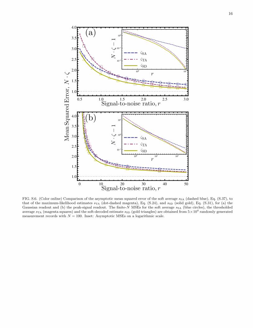
Fig. 6 compares the asymptotic performance of the soft average sSA to that of the maximum-likelihood estimates sTAand sSD as a function of the signal-to-noise ratio r, for both the Gaussian and the peak-signal readouts. As noted inRef. [29], the soft average outperforms the thresholded average sTA for low r. This is because the distribution P (O|s0)

approaches a Gaussian centered at s0 when r → 0 for both readouts, P (O|s0) '√

r2π e− (O−s0)2r

2 , and the maximum-likelihood estimator for the mean of a Gaussian coincides with the soft average. In that case, the soft average sSA istherefore the same as the soft-decoded estimate sSD. However, the soft average estimate offers suboptimal performancefor finite r and suffers from an significant loss in performance compared to sTA and sSD when r becomes large. Incontrast, the soft-decoded estimate sSD is optimal for all r.

16

FIG. S.6. (Color online) Comparison of the asymptotic mean squared error of the soft average sSA (dashed blue), Eq. (S.37), tothat of the maximum-likelihood estimates sTA (dot-dashed magenta), Eq. (S.24), and sSD (solid gold), Eq. (S.31), for (a) theGaussian readout and (b) the peak-signal readout. The finite-N MSEs for the soft average sSA (blue circles), the thresholdedaverage sTA (magenta squares) and the soft-decoded estimate sSD (gold triangles) are obtained from 5×104 randomly generatedmeasurement records with N = 100. Inset: Asymptotic MSEs on a logarithmic scale.

17

[1] J. M. Elzerman, R. Hanson, L. H. W. Van Beveren, B. Witkamp, L. M. K. Vandersypen, and L. P. Kouwenhoven, Nature430, 431 (2004).

[2] A. Morello, J. J. Pla, F. A. Zwanenburg, K. W. Chan, K. Y. Tan, H. Huebl, M. Mottonen, C. D. Nugroho, C. Yang, J. A.van Donkelaar, et al., Nature 467, 687 (2010).

[3] M. Veldhorst, J. C. C. Hwang, C. H. Yang, A. W. Leenstra, B. de Ronde, J. P. Dehollain, J. T. Muhonen, F. E. Hudson,K. M. Itoh, A. Morello, and A. S. Dzurak, arXiv preprint arXiv:1407.1950 (2014).

[4] B. D’Anjou and W. A. Coish, Phys. Rev. A 89, 012313 (2014).[5] J. Gambetta, W. A. Braff, A. Wallraff, S. M. Girvin, and R. J. Schoelkopf, Phys. Rev. A 76, 012325 (2007).[6] R. Y. Rubinstein and D. P. Kroese, Simulation and the Monte Carlo method, 2nd ed. (John Wiley & Sons, Hoboken,

U.S.A., 2008) Chap. 2, pp. 51–54.[7] In Ref. [12], a two-qubit repetition code was implemented using two trapped ions. The enhanced detection was obtained

by collecting the total fluorescence O of both ions. We note that according to Eq. (S.4), this effectively implements softdecoding of the repetition code if the fluorescence counts follow a Gaussian readout distribution. For a general readout,however, knowledge of O is not sufficient to determine ΛO; in this case the analog observable Oi must be recorded for eachqubit.

[8] W. Press, B. Flannery, S. Teukolsky, and W. Vetterling, Numerical Recipes in Fortran 77: the art of scientific computing,2nd ed. (Cambridge University Press, Cambridge, United Kingdom, 1992) Chap. 6, pp. 219–222.

[9] D. Chase, Information Theory, IEEE Transactions on 18, 170 (1972).[10] C. A. Ryan, B. R. Johnson, J. M. Gambetta, J. M. Chow, M. P. da Silva, O. E. Dial, and T. A. Ohki, arXiv:1310.6448

(2013).[11] H. Cramer, Mathematical methods of statistics (Princeton University Press, Princeton, NJ, 1946) Chap. 32-33.[12] T. Schaetz, M. D. Barrett, D. Leibfried, J. Britton, J. Chiaverini, W. M. Itano, J. D. Jost, E. Knill, C. Langer, and D. J.

Wineland, Phys. Rev. Lett. 94, 010501 (2005).