Sociology Working Papers

Paper Number 2010-01

Leisure Inequality in the US: 1965-2003

Almudena Sevilla Sanz

José Ignacio Giménez Nadal

Jonathan Gershuny

Department of Sociology University of Oxford

Manor Road

Oxford OX1 3UQ www.sociology.ox.ac.uk/swp.html

1

Leisure Inequality in the US: 1965-20031

Almudena Sevilla Sanz

Department of Economics and Centre for Time Use Research, University of Oxford (UK)

and

José Ignacio Giménez Nadal

Department of Economic Analysis, University of Zaragoza (Spain)

and

Jonathan Gershuny

Department of Sociology and Centre for Time Use Research, University of Oxford (UK)

Abstract

This paper focuses on the quality of leisure time to show that a historical equalization in the

distribution of leisure in terms of quantity has been counterbalanced to some extent by a simultaneous

increase in the unequal distribution of leisure quality. We exploit the nature of diary data in the American

Heritage Time Use Study (AHTUS) to construct three classes of indicators that capture the quality of

leisure (“leisure dilution”, “leisure fragmentation” and “co-present leisure”). Complementary evidence

on the instant enjoyment of activities is used to demonstrate that these indicators genuinely capture aspects

of leisure quality. We deploy the leisure-quality indicators to show that highly educated individuals may

now have less leisure than others, but this leisure is less fragmented, more likely to be enjoyed in the

company of other adults, and is less likely to be contaminated by simultaneous non-leisure activities. By

providing a more complete picture of how the unequal distribution of leisure in terms of quantity and

quality has evolved in the last decades for the US, our results provide a basis for interpreting inequality in

the US and for weighing the relative decline in earnings and consumption for the less educated against the

simultaneous relative growth of leisure.

JEL Classification: C13, C23, D13, J12, J16, Z13

Keywords: Leisure; Inequality; Income; Wages; Consumption; Time-Use; Time Budgets

1 The authors would like to express their thanks for the financial support provided by the Spanish Ministry of Education

and Science (Project SEJ2005-06522) and the Economic and Social Research Council (Grant number RES-060-25-

0037). Correspondence to Almudena Sevilla- Sanz. University of Oxford. Department of Economics and Centre for

Time Use Research, Manor Road Building, Manor Road, Oxford O1 3UQ (UK). Phone: +44 (0)1865 2 81740. Fax:

+44 (0)1865 2 86171. Email: almudena.sevilla@economics.ac.uk.

“The basis on which good repute in any highly organized industrial community

ultimately rests is pecuniary strength; and the means of showing pecuniary

strength, and so of gaining or retaining a good name, are leisure and a

conspicuous consumption of goods”

Thorstein Veblen (1953), Chapter 4.

1. Introduction

The unequal distribution of leisure in the US over the last four decades contrasts remarkably

with how inequality in wages and expenditure has evolved over the same period of time. Despite

growing wage and expenditure inequality in the U.S (e.g., Attanasio and Davis [1996], Autor and

Katz [1999], Krueger and Perri [2006]), the cross- sectional distribution of leisure time has

expanded over the last 40 years (Aguiar and Hurst [2007]). While the level of leisure in 1965 was

roughly equal across educational groups, the subsequent increase in leisure was greatest among

low educated adults. Thus, highly educated individuals have now less leisure time than low

educated individuals.1 This variation in leisure across educational levels has also been

documented by Gershuny [2009a]; a reversal of the previously negative relationship between

human capital and work time is found in all 11 developed economies for which comparable

historical time use data is available. Understanding why less-educated adults have increased their

relative consumption of leisure, particularly in the last twenty years, the same period in which

wages and consumption expenditures increased faster for highly educated adults, can help us in

interpreting inequality in the US and in weighing the relative growth of leisure for the less

educated against the simultaneous decline in relative wages and consumption.

In this paper we uncover the black box of leisure time and exploit the rich information in the

time-use diary data to construct three classes of indicators that capture the quality of leisure

(―leisure dilution‖, ―leisure fragmentation‖ and ―co-present leisure‖). In particular we look at the

simultaneity of leisure activities with non-leisure activities, the presence of other individuals

while the respondent is engaging in a leisure activity, and the extent to which leisure events are

interrupted by other activities. We start by validating these indicators, using, for the first time,

complementary evidence on the instant enjoyment of activities. Results from the validation

exercise show that our indicators do genuinely capture aspects of leisure quality that contribute to

enjoyment of activities beyond what is predicted by individual characteristics or the nature of the

activity. Thus, even though we lack the additional information about respondents‘ enjoyment of

1 A similar pattern is found by Costa [2000], who documents that low-wage workers reduced their market work hours

relative to high-wage workers between 1890s and 1991. In particular, at the turn of the twentieth century, low-wage

workers worked longer hours than high-wage workers. This differential disappeared by the early 1970s, and during the

last thirty years high-wage workers supplied relatively more market hours.

1

activities across the historical period being analyzed, the diary still provides direct information

that can be used in a well-crafted empirical decomposition of trends in the quantity and quality of

U.S. leisure time. Based on these leisure-quality indicators, we show that the decrease in the

unequal distribution of leisure in terms of quantity has been counterbalanced to some extent by a

simultaneous increase in the unequal distribution of leisure in terms of quality.

By providing a more comprehensive account of leisure, our work adds to the existing

literature on measuring changes in the allocation of time in the US. This literature mainly

concentrates on the study of aggregate times (e.g., Ghez and Becker [1975], Juster and Stafford

[1985], Robinson and Godbey [1997], and Aguiar and Hurst [2007]). However, introducing other

dimensions of time in the analysis of inequality is crucial. Although the scarcity of leisure time

may seem analogous to income poverty, in that both reflect the scarcity of resources, the two

concepts have different dynamics. In a growing economy the goods constraint relaxes over time,

whereas the 24 hours per day time constraint, does not. We propose in what follows that the time-

budget constraint can however be ameliorated by adjusting the quality of leisure over time.

There are different ways of assessing the quality of leisure. One methodology is to use self-

reported measures of how enjoyable activities are. This is the spirit of the related albeit distinct

approaches described in the literature respectively as process benefits and experienced utility. The

former uses time-diaries in combination with a separate questionnaire containing self-assessment

of enjoyment of specific activities, to estimate individuals‘ subjective well-being (see Juster et al.

[1985]). The latter uses diaries as the source of information on both activity durations and

enjoyment levels (see Robinson [1993], Gershuny and Halpin [1996], Sullivan [1996a,1996b],

and Kahneman and Krueger [2006] among others). The experience sampling method, which

consists in asking the individual about his or her emotions at the moment or shortly after the

event happens, is the optimal approach to capturing an individual‘s instant enjoyment of an

activity, but this method imposes a considerable burden on respondents, and can only be used to

capture a few disconnected activities in the course of a day. The ―yesterday‖ diary method (also

described as the ―day reconstruction method‖ by Kahneman et al [2004]) in which respondents

record their recollections of their affective responses within 24 hours of the actual events, is

probably the best currently available compromise.

Though we have a historical series of representative diary samples for the US (and for many

other countries), only one of the US surveys (and one similar UK survey) contains information

about instant enjoyment levels for a nationally representative sample. We thus propose an

approach complementary to experienced utility that uses the rich information in the existing US

2

time-use diary series to measure the distribution of quantity and quality of leisure across

education groups in the last decades. The diary records allow us to look, beyond the total times

spent in a given activity, to the event level indicators of diary quality described briefly above.

These leisure-quality indicators emerge independently from different strands in the socio-

economic and psychological literature. The relationship between quality of leisure and some of

these indicators, in particular those related to the presence of other individuals while the

respondent engages in leisure activities, has been directly established using instant-enjoyment

data of the sort proposed by the experienced-utility literature (Sullivan [1996a,1996b], Kahneman

et al [2004]). The other two sorts of indicator are discussed in prior literature (e.g., Bittman and

Wajcman [2000], Bianchi et al [2006]), but have not been directly validated through comparison

with enjoyment evidence. In what follows we validate the indicators using (inter alia) the under-

exploited diary-derived instant enjoyment rating of activities in the 1985 component of the

AHTUS (e.g., Robinson [1993]). We show that these indicators very effectively capture the diary

respondents‘ descriptions of their own enjoyment of activities. Enjoying uncontaminated leisure,

spending leisure time in the company of the spouse and other adults, and having less fragmented

leisure all emerge as contributing to higher levels of enjoyability of activities. These results hold

even after controlling for individual characteristics and the type of activity being done—implying

in turn that our indicators alone are capable of conveying the great majority of the information

about leisure quality.

Our indicators of leisure quality show that, despite increases in the quantity of leisure over

this period (as reported by Aguiar and Hurst [2007] and others, and confirmed in Section 5

below), the quality of leisure has decreased for all groups. This result may help explain the fact

that, despite general increases in leisure time, Americans report an increased feeling that leisure

time has become scarcer and more harried compared to forty years ago (e.g., Hamermesh and Lee

[2007], Robinson and Godbey [1997], Schor [1993]). However, the focus of this paper is a

comparison across educational groups over time. It emerges that, despite highly-educated

individuals now having less leisure time, they enjoy a higher quality of leisure than less-educated

individuals.

After controlling for demographic and socio-economic characteristics, we find that low

educated men, and to a much greater extent women, have increased the quantity of leisure

significantly more than highly educated individuals over this period. Leisure time increases half

an hour per week more for low educated men than for highly educated men, and increases three

and a half hours more for low educated women than for highly educated women. These

3

differences however are reversed when we look at the quality of leisure. Leisure dilution (the

amount of leisure time that is not ―contaminated‖ by other non-leisure activities) declined much

more for low educated individuals (about one and a half hours as opposed to just one hour for

highly educated individuals). Co-present leisure also declined less for highly educated individuals

during this period. Whereas highly educated men and women experienced almost no decrease in

the time spent with the spouse, low educated individuals experienced a one-hour decrease of co-

present leisure time. Leisure fragmentation also increased more for low educated individuals than

for highly educated individuals. Our results show that low educated adults are more likely to have

shorter leisure spells and more leisure intervals than highly educated individuals.

We further look at whether increases in the time spent watching television may have

contributed disproportionately to the unequal distribution of leisure. We focus on this activity

because it represents the largest single part of total leisure time, and has increased substantially

over this period, particularly for low educated individuals. TV watching also ranks particularly

low in terms of our quality indicators. We show however that the pattern of change of leisure

quality (and quantity) across educational groups remains very similar when TV watching is not

included in the definition of leisure. We also look at other leisure activities, ‗At Home Leisure’

and ‗Read/Listen’, which also represent a significant amount of leisure time. We find that these

activities cannot entirely explain the pattern in the unequal distribution of leisure quality across

educational groups either.

This paper is organized as follows. Section 2 describes the time-use datasets used in the

analysis. Section 3 provides a conceptualization for the quantity of leisure, and presents the

theoretical and empirical underpinnings for our leisure-quality indicators. Section 4 validates our

leisure-quality indicators using additional diary information on instantaneous enjoyment. Section

5 presents the empirical strategy and the main results. Section 6 looks more deeply into how the

nature of specific leisure activities may have contributed to the unequal distribution of leisure in

terms of quantity and quality, and Section 7 concludes.

2. The American Heritage Time Use Study (1965-2003)

We use the American Heritage Time Use Study (AHTUS) in our main analysis. The AHTUS

is a harmonized dataset that covers five decades, from 1965 to 2003, over five time-use surveys.

Appendix A Table A1 describes the five surveys in the AHTUS. The harmonization exercise is

comprehensively documented in Fisher et al. [2006], and the resulting data is freely

4

downloadable from www.timeuse.org. The harmonization exercise was commissioned by

Professor William Nordhaus at the Yale University Program on Non-Market Accounts, from the

Centre for Time Use Research (now in Oxford University, then at the University of Essex), and

funded by the Glaser Progress Foundation. The harmonization project involved a great deal of

effort due to the heterogeneity of the time diary datasets, and was peer-reviewed by a

multidisciplinary body of time-use scholars, whose suggestions where incorporated into the final

version of the dataset.2

While the time diary studies from 1965 forward have some common elements, they vary in

terms of data quality. The two best data sets for our purposes are from 1975 and 2003. The 1975

study was reasonably funded and great attention was paid to the sampling and administration of

the diaries to respondents (or respondent-spouse pairs in the case of married couples). The 2003

data from the American Time Use Survey are also of high quality, although they do have the

anomalous absence of secondary activities. The 1965 data were a part of a multinational study

and are restricted to urban areas of the US and had very low granularity in the diary coding (i.e.,

the categorization of activities was broader than later surveys).3 The sample is also small. The

1985 and 1993 studies were funded at low level and included sampling and data quality

compromises such as the use of mail back questionnaires.4 Nevertheless, we have used all these

data sets; the fact that the 1975-2003 pattern of change is consistent with that including the other

surveys, particularly since the paper is based on fairly specialized constructions of the underlying

diary activity records, makes us confident that we have identified real changes in the quality of

leisure time.

2 Among the reviewers are Dr Dorinda Allard (Bureau of Labor Statistics); Professor Michael Bittman (University of

New England); Professor Barbara M. Fraumeni (University of Southern Maine); Professor Daniel S. Hamermesh

(University of Texas at Austin); Professor Andrew Harvey (Saint Mary's University); Dr Diane Herz (Bureau of Labor

Statistics; Professor J. Steven Landefeld (Bureau of Economic Analysis); Dr Jay Stewart (Bureau of Labor Statistics);

Dr Hidde van der Ploeg (University of Sydney); and Dr Vanessa Wight (University of Maryland). See reference on the

AHTUS.

3 While it is true that the 1965 Szalai Surveys contain fewer categories than ATUS, for instance, it is also true that the

ATUS does not have many more useful categories than Szalai - there are some about security procedures, but the

myriad of sports participation codes, fine detail shopping codes, fine detail household maintenance codes and the like

are not commonly used in research as so very few respondents record these precise activities in their diaries. In

practice, researchers collapse to much broader categories.

4 Mail-back diaries are lower quality as respondents completing them are not expert in the diary process, and they make

mistakes that impact diary quality. When a survey leaves behind a diary and the interviewer comes to collect the diary

and goes over the entries with the diarist in person (HETUS, the USA 1975, the Szalai 1965 surveys, for example), the

interviewer can identify mistakes and clarify and fix the entries with the diarist. Web-based diary collection and CATI

(as is used in the ATUS and NHAPS) achieve similar quality improvements because the script prompts correction of

common mistakes - such noting to the diarist -you make no mention of eating or drinking during the day. Are you sure

that you did not eat or drink anything? or you reported being at your home at 8:45, and by 9:00 you say that you were at

your workplace, yet you did not report any form of travel between these two places. How did you get from your home

to your workplace, and when did you make this journey? (see Szalai [1972], Juster and Stafford [1985], Staikov [1989],

Kalfs and Saris [1997]).

5

The main instrument of all the surveys is an activity diary in which respondents record what

they do for a consecutive period of 24 hours. The advantage of the AHTUS over other U.S.

harmonized surveys used in previous studies for the same period is that, whereas most surveys

simply cover the total minutes per day diarists recorded in the main activity columns, the AHTUS

harmonizes these surveys at the episode level, so that for each respondent there is a diary file

made up of a sequence of episodes over the 24 hour span. The AHTUS also includes harmonized

information on secondary activity, location, mode of transport, and who else is present at the time

of the activity.

For the sake of comparison with previous studies, and to minimize the role of time allocation

decisions that have a strong inter-temporal component over the life cycle, such as education and

retirement, we restrict the sample used throughout the analysis to non-retired/non-student

individuals between the ages of 21 and 65 (inclusive), so results should be interpreted as being

―per working-age adult‖ (or per adult within the specified sub-sample, when relevant). This

approach also avoids possible biases from the changing proportion of retired individuals in the

general population over this long period. Not including individuals out of the labor force however

may be particularly problematic if low educated individuals are more likely to be non-employed

and thus have a higher amount of leisure. This is a problem that we share with previous studies

that look at trends in the amount of leisure. The fact that we control for total leisure time in our

analysis makes this issue less problematic for our indicators of leisure quality, although a possible

bias remains if low educated individuals are more likely to be retired and if leisure time during

retirement is of lower quality. In that case we would be underestimating the real inequality in

leisure quality and the difference between low and high educated individuals with respect to the

quality of leisure would be even greater. We have conducted robustness checks including retired

and non-retired individuals between 24-65 and 24-72 years old. Results do not change (available

upon request).

We also restrict the sample to include only individuals who have time diaries that add up to a

complete day (1440 minutes) and whose diary is not low quality, i.e., the diary has 90 minutes or

less missing main activity time (that is they have accounted for the majority of the day), and it has

seven or more episodes. The seven episode cut-off seems realistic. Most respondents have at least

one sleep or rest episode, at least two different eating or drinking episodes, at least two different

personal care episodes, and at least two episodes of some other activities. The excluded diaries

represent only 3 per cent of the age 21-65 sample and results are robust to their inclusion.

6

The final sample does not include those individuals whose diary includes some time recorded

in at least three of four basic activities (sleep or rest, eat or drink, personal care, and travel) as a

primary or secondary activity (or in the case of travel, marked through location of means of

transport). Some respondents providing child-care to multiple children, or to an infant, as well as

some diarists performing adult care did not record travel and also missed a second or third basic

activity. If these diaries from carers nonetheless included at least 10 episodes, then we counted

these diaries as good diaries (as it may be possible the diarists ate while feeding the care recipient,

for example, but did not record her or his own eating). These diaries represent 7 per cent of the

sample aged 21-65, and results are again robust to their inclusion.

3. Indicators of the Quantity and Quality of Leisure

3.1. Conceptualizing the Quantity of Leisure

The conceptualization of time use categories is sometimes based on groupings of diary

activities (such as watching television, working for pay, or doing laundry) relying on researchers

ad hoc judgments. These introspection-based judgements may be driven by arbitrary and partial

views about the pleasure to be derived from different activities. But enjoyment may be derived

directly from non-leisure activities; and some leisure is duty not pleasure. So this approach is less

than entirely satisfactory.

The more systematic, principle-driven approach of distinguishing means vs. ends might

initially seem more satisfactory. The third person criterion excludes activities that might be

carried out by some third party without losing the intended utility for the final consumer. We can

either cook or pay someone to cook for us; we must watch the television for ourselves. Work time

is, according to this criterion, perfectly substitutable by purchased goods and services without

loss of the final utility provided by the ultimate consumption commodity. But does this really

provide a more objective conceptualization of leisure? Unfortunately, it involves similarly

questionable assumptions about the association of utilities with activities—that the enjoyment

derived from work can legitimately be ignored, and that all leisure is enjoyable.

To what extent does the set of activities that are normally assumed to be leisure according

to the third person criterion correspond to activities that are actually considered as leisure? Young

and Willmott [1973] collected diaries which link information about activity sequences and

timings to simultaneous subjective judgments about whether each activity was to be considered as

leisure, work, both or neither. One quarter of time that would be considered leisure according to

7

the conventional implementation of the third person criterion, and one third of what would

conventionally be considered work, is unexpectedly placed by the diarists (Gershuny [2009b]).

A further problem with the third person criteria is that certain activities, such as sleeping,

eating, personal and medical care, or resting, do not fall comfortably into the means vs. ends

classification. These activities cannot be purchased in the market, so they may not be considered

leisure in the sense that they are necessary for life. They are thus normally included in a different

category of time use - either referred to as ―personal care‖ (e.g., Aguiar and Hurst [2007]) or as

―tertiary activities‖ (e.g., Burda et al. [2008]) and they are not included as leisure in what follows.

Nonetheless, some variation in the time spent in these activities may result from conscious

choice. For example using data for the Netherlands, Hamermesh [2002] shows that when moving

the clocks back to standard time, the additional hour is almost entirely used for extra sleep.

Similarly, Biddle and Hamermesh [1990] show that sleep time, similarly to other uses of time

such as time in market work and more standard leisure activities, responds to economic incentives

such as the wage. Decreasing marginal utility to sleep (and other consumption activities) is

indeed shown by Gershuny [2009b] who uses (subsequent) diary reports of enjoyment to show an

inverted-U shaped relationship of reported enjoyment to sleep duration.

Rather than trying to resolve this debate on theoretical grounds, we have adopted a

empirical approach, exploring four commonly used, nested, definitions of leisure, ranging from

the narrow (which includes activities designed to yield direct utility such as entertainment,

socializing, active recreation, and general relaxation), to the broad (time spent neither in market

production nor in nonmarket production). The various measures tell a consistent story, so for the

sake of brevity we present here only the results regarding our narrowest measure of leisure, i.e.,

hours per week devoted to all activities that we cannot pay somebody else to do for us and that

are not biological needs (e.g., Walker and Gauger [1973], Hawrylyshyn [1976,1977], Burda et al.

[2008]).5 Table A2 in Appendix A lists all the activities included in the AHTUS, as well as those

activities that we consider leisure activities based on the definition above. Among the activities

included in the leisure category are watching television, sport activities, general out-of-home

leisure activities, and socializing.6

5 Results for the other definitions of leisure are available upon request.

6 We exclude voluntary activities from our main definition of leisure, since it really classes as work under the third

person criterion (see Hawrylyshyn [1976]). The validity tests presented in Section 4 clearly show that voluntary

activities rank with work rather than leisure activities.

8

3.2. Conceptualizing the Quality of Leisure

There are different ways of assessing the quality of leisure. One methodology is to use self-

reported measures of how enjoyable activities are, in the spirit of the process benefits and

experienced utility literature. Juster and Stafford [1985] define process benefits as the ―direct

subjective consequences from engaging in some activities to the exclusion of others‖.7 Going

back to the earliest conceptions of utility, from Jeremy Bentham through Francis Ysidro

Edgeworth and Alfred Marshall, the concept experienced utility has been proposed more recently

by Kahneman et al [2004] to refer to a ―continuous hedonic flow of pleasure or pain‖.

Both lines of research use time-use diaries together with information on enjoyment to assess

individuals‘ subjective well-being. The process benefits approach uses Activity Enjoyment

Ratings, where respondents are to rate on a scale from 0 to 10 how much they generally enjoyed a

type of activity (e.g., Juster and Stafford [1985]). The information gathered this way offers a

global and retrospective interpretation of feelings about activities, although they may not serve as

a good predictor of the instantaneous satisfaction experienced in any given instance of the activity

(Gershuny and Halpin [1996]). The experienced utility literature has proposed the Experience

Sampling method as a superior way for collecting objective instantaneous enjoyment data. As

opposed to the Activity Enjoyment Ratings, the Experience Sampling method collects information

on hedonic experiences (or instant enjoyment) in real time. It has however never been applied to a

representative population sample because it is extremely burdensome for the respondent.8

Alternative methods of collecting data on hedonic experiences, such as the conventional

yesterday diary used in time budget surveys (Szalai [1972]) or the Day Reconstruction Method

(Kahneman et al. [2004b]) are less costly to implement. Both methods collect information on how

the respondent experienced all or some of the activities he or she engaged in during the previous

day, as described by a time-use diary.9

7 ―For instance, how much an individual likes or dislikes the activity ‗painting one‘s house,‘ in conjunction with the

amount of time one spends in painting the house, is as important determinant of well-being independent of how

satisfied one feels about having a freshly painted house.‖ (Juster and Stafford [1985])

8 Experience sampling was developed to collect information on people‘s reported feelings in real time in natural

settings during selected moments of the day (Csikszentmihalyi [1990], Stone and Schiffman [1994]). Participants in

ESM carry a handheld computer that prompts them several times during the course of the day (or days) to answer a set

of questions immediately, such as their physical location, the activities in which they were engaged just before they

were prompted or the people with whom they were interacting. They also report their current subjective experience by

indicating the extent to which they feel the presence or absence of various feelings, such as feeling angry, happy, tired

and impatient (Steptoe, Wardle and Marmot [2005], Kahneman and Krueger [2006]).

9 The Day Reconstruction Method has been used for example in the collection of the Princeton Affect and Time Survey

(PATS). Here respondents were asked to reconstruct the previous day by completing a short diary. Then three 15-

minute intervals were randomly selected from the non-sleeping portion of the diary, and respondents were then asked

the extent to which they experienced six different feelings (pain, happy, tired, stressed, sad, and interested) during each

9

In what follows we adopt a complementary approach to the above literature. We exploit the

rich information in the diary to construct three classes of indicators that capture leisure quality.

Leisure dilution

The first class of indicator is related to the nature of the secondary activity that is combined

with leisure as a primary activity. The primary activity constitutes the main activity the

respondent engages in at a particular point in the diary. However, respondents frequently engage

in more than a single activity at the same time. The secondary activity is the activity that is done

at the same time as the main activity, and complements the main activity. The underlying

rationale behind this indicator is that leisure activities with no ―distracting‖ accompanying

activities are associated with a higher utility than leisure activities accompanied by a secondary

activity (see Bittman and Wajcman [2000], and Mattingly et al. [2003]). We thus define Pure

Leisure as leisure that is reported as primary activity whose secondary activity is also leisure, i.e.,

its secondary activity is not market work, home production or personal care and analyze the

proportion of Pure Leisure out of total leisure. Pure Leisure cannot be analyzed for 1993 and

2003 since in these surveys there are no reported secondary activities as such. Although these

secondary activities were imputed by the survey team, even after the imputation exercise

important differences still remain. In particular, the 1993 and 2003 surveys have no more than 4

secondary activities, compared to up to 80 secondary activities in the 1965, 1975, and 1985

surveys. This makes these surveys not comparable with the previous surveys (see Fisher et al.

[2007]).

Co-present leisure

The second class of indicators relates to with whom the leisure activity is performed. We first

consider leisure with the spouse (or partner). The concept of Leisure with Spouse draws from the

empirical evidence found in the socio-economic literature on spouses‘ synchronization of work

and leisure activities. Sullivan [1996a] uses the 1985 UK time-use survey, a diary survey with

instant enjoyment information, to show that partners report higher levels of satisfaction when they

synchronize their working schedules (and thus maximize the potential time they can spend in

interval (Krueger [2007]). Previously, the Yesterday Diary was used to collect information on the levels of instant

enjoyment for all the episodes (not just three) in the diary in the UK Data and the US AHTUS data used in Section 4 of

the present paper. Unlike the PATS, these surveys collect one dimension of instant enjoyment, which is scaled from 0

to 5 and 0 to 10 respectively.

10

leisure activities together).10

Hamermesh [1999], Hallberg [2003], and Jenkins and Osberg [2005]

find that synchronization of leisure activities between partners is indeed greater than random

male-female pairing would predict. We thus use information on whether leisure as primary

activity is carried out while the spouse/partner is present to look at the percentage of total leisure

time of Leisure with Spouse (or partner) as an indicator of leisure quality. Because of

demographic changes regarding the propensity to marry, which has fallen in the US during this

time period due to the delay in the age of marriage and increase in divorce rates, we restrict the

sample to those individuals with a partner when computing this indicator. The indicator of leisure

with the spouse can be constructed for all the surveys except for those in 1985 and 1993, because

information on whether the spouse or partner is present at the time the main activity is carried out

by the respondent was not gathered.

The second indicator in this class uses information on whether another adult was present

during a leisure activity to construct the percentage of total leisure that constitutes Leisure with

other Adults, i.e. leisure time spent with non-partner adults (neither alone nor in the presence of

children).11

We can calculate this indicator for the 1965, 1975, and 2003 surveys. There is

evidence from instant enjoyment data, which suggests that individuals report higher levels of

instant satisfaction from activities done in the company of others than by themselves (e.g.,

Kahneman et al [2004], Helliwell and Putnam [2005]). In fact the adverse effects of isolation on

mental health is well-known in the epidemiological and psychological literature (e.g., House et al.

[1988], Berkman and Glass [2000], Putnam [2000], Eng et al. [2002], Berkman et al. [2004], and

Singh-Manoux and Marmot [2005] among others). Similarly, the positive externalities of

synchronicity not just in leisure, but also in market work and household labor, have been often

pointed out in the economics literature (e.g., Weiss [1996]). Few studies have tried to identify

exogenous determinants of coordination. For example, public holidays have been found to be

welfare enhancing, not only by increasing the amount of leisure to each individual, but also

increasing the coordination of leisure activities among individuals (e.g., Mers and Osberg

[2006]). Similarly, Hamermesh et al. [2008] find that an exogenous shock to time in one area, due

10 There is extensive evidence pointing toward positive assortative mating along education (Lam [1988], Blosfeld and

Timm [2003]) and it thus may well be that highly educated individuals have a higher preference for spending leisure

time with a spouse, precisely because the spouse is also highly educated. This hypothesis does not seem to be ratified

by the results shown in Section. We find that individual‘s enjoyment of leisure time when accompanied by the spouse

is greater regardless of educational class.

11 The category ―other adult‖ is considered to be the spouse or partner, other adult from the household, a shop or

professional worker, a co-worker, a person well-known, and other (adult) person present. Unfortunately, the AHTUS

lacks comparable information across years on whether a child is present, and thus comparisons along these lines are not

possible.

11

to daylight-saving time, leads its residents to change their work schedule to be able to coordinate

their other (leisure) activities with those in adjacent areas. They also find that workers in

industries who are expected to have a greater coordination with individuals in other areas are

more responsive to exogenous changes in time zones.

Leisure fragmentation

The third class of indicators refers to the fragmentation of leisure activities. The first indicator

within this class uses the episode-level information in the data to investigate to what extent

leisure is fragmented during the course of the diary day. For a given amount of leisure time, those

individuals with more fragmented leisure may be justifiably more rushed and stressed. Beyond

feeling of stress, the more activities people fit into a single day, the less time they have to fully

engage with each individual activity, and thus might enjoy a lower level of utility from any given

amount of leisure time if they do not get what they want out of their leisure when trying to

accomplish too much and not having proper time for any one activity.

To measure the fragmentation of leisure we use the number of leisure intervals during the

diary day. An interval is defined as a period of time when the individual is engaged in one of

these four main activities: market work, personal care, home production and leisure. We then

define a leisure interval as that time interval where the main activity is leisure (regardless of

whether the interval contains two or more different leisure episodes).12

The switch of method

from the diary the diarist sees (1965, 1975 and 1985) to the telephone diary (1993 and 2003)

seems to have resulted in a decline in the number of episodes in recent surveys. Also for the

earlier studies (1965, 1975 and 1985) respondents are automatically assigned a new episode with

a change of location, main activity or secondary activity, which results in these surveys having

more episodes. Because of this general decrease in the mean number of intervals reported by

individuals over the five surveys, we normalize this measure by dividing by the total number of

intervals in the diary for each respondent.

One concern with the above indicator is that fragmentation may be one measure of variety

(imagine having one twelve-hour leisure episode vs. two six-hour episodes), and there is cross-

section evidence that higher-income people prefer and obtain variety (Gronau and Hamermesh

[2008]). In order to address this concern we construct another indicator of the fragmentation of

12 The diary survey is organized in episodes. Thus, two consecutive leisure activities are considered to be different

episodes (i.e. reading and cycling), but these consecutive leisure episodes are considered to be the same leisure interval

according to our definition.

12

leisure by looking at those individuals with an average duration of leisure episodes below half the

median duration for each year. This indicator is akin to an income poverty measure, but measures

the poverty in the duration of leisure intervals instead. Practically what this means is that for each

individual, this indicator takes value ―1‖ if the average duration of leisure episodes is below half

the median duration for that survey year, and ―0‖ otherwise.

3.3. Unconditional Trends in the Quality and Quantity of Leisure

Table 1 shows the main summary statistics for the indicators of quantity and quality of leisure

over the sample period for men and women separately.13

Despite increases in the quantity of

leisure for both men and women, the percentage of Pure Leisure, the percentage of Leisure with

Spouse, the percentage of Leisure with Adults, and the two indicators related to the fragmentation

of leisure seem to reflect a decrease in the quality of leisure.

For men, the quantity of leisure is similar to that found in other papers.14

Total hours of

leisure per week exhibit a statistically significant increase over the period of reference, from 28

hours of leisure per week in 1963 to 33 and a half hours of leisure per week in 2003 (leisure

increases by 5 hours and a quarter per week).15

The quality of leisure time decreases over this

period however. The percentage of Pure Leisure out of total leisure time decreases over the

period by 5 percentage points, from 89 per cent in 1965 to 84 percent in 1985. There is also a

statistically significant decrease of 14 percentage points in 2003, with respect to 1965, in the

percentage of leisure time spent with the spouse, from 49 per cent in 1965 to 35 per cent in 2003.

Similarly, the percentage of Leisure with Adults decreases by 13 percentage points in 2003, with

respect to 1965, from 73 percent in 1965 to 60 percent in 2003. Finally, the fragmentation of

leisure measured by the normalized number of leisure intervals and the duration of leisure

intervals indicates that leisure is more fragmented now than four decades ago. There is a general

increase in the number of leisure intervals (from 23 in 1965 to 25 in 2003), while the percentage

13 We use the weights provided in the AHTUS. These weights account for population/sample distribution by age group

and se, and provide an even distribution of the days of the week. All cases with missing basic information or bad

diaries are 0-weighted, and thus are excluded from the analysis. Further information on these weights can be found in

the AHTUS codebook at http://www.timeuse.org/ahtus/documentation/docs/pdf/Codebook.pdf.

14 Aguiar and Hurst [2007] find that leisure for men increased by 6-8 hours per week from 1965 to 2003. Burda et al.

[2008] find a decrease in the amount of leisure time in 2003, with respect to 1985, of 2.7 minutes per day, while we

find an increase of 9.51 minutes per day (1.11 hours per week). However, the sample used in their analysis is different

(20-74 years) and the authors acknowledge that over longer periods leisure has increased.

15 A p-value lower than 0.05 means a 95 per cent confidence level.

13

of individuals with a mean duration of leisure below half the median for the corresponding year

has significantly increased between 1965 and 2003 from 4 per cent in 1965 to 7.5 per cent.16

Women‘s leisure time follows a similar pattern to that of men‘s. The quantity of leisure time

significantly increases by three and a half hours over the period, from 27 hours in 1965 to 30

hours and a half in 2003.17

The quality of leisure time for women tells a similar story to that of

men‘s. The percentage of Pure Leisure decreases over the period by 6 percentage points, from 88

percent in 1965 to 82 percent in 1985. Despite increases in total leisure time the percentage of

Leisure with Spouse decreases by 4 percentage points over the period, from 35 per cent in 1965 to

31 percent in 2003. There is also a statistically significant decrease of 7 percentage points in

2003, with respect to 1965, from 68 percent in 1965 to 61 per cent in 2003. There is a statistically

significant increase in the normalized number of leisure intervals (from 20 in 1965 to 23.5 in

2003), which indicates that leisure for women is also more fragmented now than it was in 1965.

Additionally, the proportion of women with an average duration of leisure intervals below half

the median has increased between 1965 and 2003 from 4 per cent in 1965 to 10 per cent.

The evolution of leisure quality shown here is consistent with the results using instant

enjoyment data. Krueger [2007] finds that the time spent in the sorts of activities labeled

enjoyable and engaging forms of leisure according to a 2006 diary survey has decreased for both

men and women between 1965 and 2003. Our indicators do indeed suggest that, on average, the

quality of leisure that individuals enjoy is lower now than it was in 1965. This result may help

explain the fact that, despite general increases in leisure time, Americans report an increased time

stress now, compared to forty years ago. For example, when responding to the question ―Would

you say you always feel rushed, even to do the things you have to do, only sometimes feel rushed,

or almost never feel rushed?‖, the proportion of 18-64 years old who report always feeling rushed

rises from 24 percent in 1965 to 28 percent in 1975, leaps to 35 percent in 1985 and reaches its

peak of 38 percent in 1992, before declining slightly in 1995 (Robinson and Godbey [1997]). The

suggestions that Americans are feeling more pressured with time and have less social interaction

(e.g., Schor [1993] and Hochschild [1997]), and that they feel leisure time has become scarcer

16 Median values of leisure episodes duration are 30 minutes in 1965, 1975 and 1985, 60 minutes in 1993 and 45

minutes in 2003. The last two numbers reflect the decrease in the number of episodes in the latter surveys due to a

change in the survey methodology. The normalized number of intervals has been multiplied by 100 throughout the

paper in order to get figures with only one decimal positions.

17 Aguiar and Hurst [2007] find that leisure for women increased by 4-8 hours per week over the period 1965-03. Burda

et al. [2008] find a decrease in the amount of leisure time in 2003, with respect to 1985, of 13.3 minutes per day, while

we find an increase of 7.54 minutes per day.

14

and more harried (e.g., Frederick [1995], Linder [1970]), may thus have more to do with the

quality of that leisure than with the total time spent in leisure activities.

4. Validating the four classes of indicator

As seen in Section 3.2, all three classes of indicators emerge independently from different

strands in the socio-economic and psychological literature. The relationship between quality of

leisure and some of these indicators, in particular those related to the presence of other

individuals while the respondent engages in leisure activities, has already been directly

established using instant-enjoyment data of the sort proposed by the process-benefits and

experienced-utility literature. However, how the rest of the indicators relate to the quality of

leisure has remained elusive in the literature. To avoid a black-box argument in our exposition,

we first test and validate these indicators together, partly from the AHTUS itself, partly from a

closely analogous dataset.

The 1985 element of the AHTUS did not include the ―with whom?‖ diary information for

each registered event. But the 1985 sample used in the AHTUS did collect an additional item of

information not available elsewhere in the sequence of surveys: an activity enjoyment ―rating‖

(on a 0-10 ―dislike it‖/ ―like it‖ scale) attached to each event (see Robinson [1997]). A similar

diary dataset (though rating activities on a 1-5 ―like it‖/ ―dislike it‖ scale, and collecting

information on a fixed 30 minute grid, rather than the open intervals used in the US survey), from

a national random sample of individuals living as members of heterosexual couples in the UK in

1986, does include co-presence data (see Sullivan [1996a,1996b]).

The validation consists of a demonstration, through a simple OLS regression, that our leisure-

quality indicators are indeed associated with diary respondents‘ descriptions of their own

enjoyment of activities.18

We select the same age range from the two samples (18-72, slightly

broader than that used elsewhere in this paper), and consider just those US diarists with co-

resident partners, so as to produce event-level datasets with 54,854 cases for the US and 47,407

cases for the UK. We estimate the following equation on the event level datasets (i.e., case =diary

event), weighting the cases by the duration of the event:

18

An alternative method would require imputations of enjoyment-levels for the other survey years (either at the activity

level as in Krueger [2007] or at the individual level). A potential limitation to this method (see Krueger [2007]) is that

it maintains the nature of activities relatively constant, not only over time, but also across educational groups. This

latter point is particularly relevant in the current context, as different groups of individuals may rank the same activity

differently, and the mix of these responses may change over time. The results from our validation exercise suggest that

our indicators can still be used as a good proxy for leisure quality. We thus leave investigating this alternative method

for future research.

15

jijiijijiji AXDIE ,,43,2,1, (4.1)

where i is the individual (or a diary) and j is the episode in the diary characterized by a unique

primary activity. The dependent variable jiE , is the activity enjoyment ―rating‖. A linear

transformation ((5.5-rate)*2) of the UK activity rating scores produces a 5 point, 1-9 positive

scale centered similarly to the US rating. Treating the rating scales (for the purpose of this

validation exercise but not elsewhere in this paper) as if they have equal intervals, the

transformed UK ratings mean score is of 6.86 and standard deviation of 2.13, which compares

neatly with the US mean of 6.99 and standard deviation of 2.43. The UK survey collected 5 days

of data from each diarist, we thus present the more conservative robust standard errors clustered

at the respondent level as the basis for significance testing.

The vector jiI , contains five leisure-quality indicators as described in Section 3.2. In

particular the vector contains a dummy variable indicating whether the episode of leisure is being

done at the same time as a work activity, whether a particular leisure episode is being done with

the spouse, and whether it is being done with other adults. It also contains the number of leisure

episodes and the mean uninterrupted duration of leisure episodes in the diary. Unlike the first

three indicators, the latter two are constant throughout all the episodes in a given diary because

they are calculated across the events of the day, and then distributed to each of those events.

The vector jiD , includes two additional dummy variables, indicating respectively primary

sleep or personal care, and primary paid or unpaid work, to ensure that the default state against

which the 0/1 variables are compared is unambiguously identified as primary leisure activities

unaccompanied by secondary work. The vector iX includes socio-economic variables of the

individual, which include age, age squared, sex, an indicator variable for part time and full time

work, an indicator variable that takes value one if there is a child under 5 at home, and another

indicator variable that takes value one if there is a child between 5 and 18 years old living in the

household. The vector jiA , includes five dummy variables indicating the nature of the leisure

activity being done. These are classified into out of home leisure, active sport and exercise, read

and listening to music, watch television, and writing. Table B1 in Appendix B presents a

description of the variables used in the analysis in these two surveys.

We first estimate Equation (4.1) including neither the socioeconomic characteristics of the

respondent nor the specific nature of the leisure activity that the respondent is engaged in at a

particular period. Columns 1 and 2 in Table 2 show the associations between the leisure-quality

16

indicators and the enjoyment scores in the US and the UK data respectively. It emerges that these

indicators are all associated with the activity enjoyment ratings in the expected directions with the

single exception discussed below. Notice in particular the pairing of the positive effects of the

mean uninterrupted length of leisure periods, with the negative effects of the number of distinct

periods—providing strong support for the ―dislike fragmentation‖ hypothesis. The US

coefficients are also reasonably similar to the UK coefficients—with the exceptions of leisure

simultaneous with work (paid or unpaid) which is substantially negative and statistically

significant for the US, but positive, smaller, and not significant, for the UK. We can, with a fair

degree of certainty trace this to the difference in data collection methods. This indicator captures

in effect a leisure period interrupted by some form of work, and is much more likely to be

recorded in the more sensitive US open interval recording scheme, than it is with the broader-

brush UK 30 minute fixed intervals. We also suspect that the more negative UK evaluation of the

sleep or personal care events may be related to the fact that the data were collected by the UK

cosmetics-to-soap Unilever Corporation, and drew respondents‘ attention specifically to

recording instances of bathing, showering and other personal activities.

The standard deviations of the US and UK activity-enjoyment means are 2.43 and 2.13

respectively. So in the US, the average work event, according to Table 3, is enjoyed on average

.68 of a standard deviation (1.66/2.43) less than the average leisure event, controlling for the

effects of the other independent variables, and a consolidation of leisure episodes from 6 to 4,

accompanied by an increase of the mean length of a leisure episodes from 2 to 3 hours, would

increase the enjoyment by one-and-a-quarter standard deviations (i.e. ((0.05*60)+(-0.04*-

2))/2.43)). These are not insubstantial effects.

The final column of Table 2 adds in the co-presence indicators to the regression equation for

the UK sample. Leisure time with the spouse and other adults are both strongly positively

associated with enjoyment of the activities, as we hypothesized. The inclusion of the co-presence

indicators in the regression equation does not substantially change the effects of the

fragmentation measures, which suggests that these two sorts of effects operate independently of

each other. Because we lack information about the presence of children, we cannot distinguish

between time alone or time with children. Nonetheless, these results seem to suggest that, as

found elsewhere in the literature, leisure with other adults and/or with one‘s spouse is not only

more enjoyable than leisure alone, but also more enjoyable than leisure with children (Kahneman

et al [2004]).

17

That time with adults is enjoyed more than time with children might seem opposed to the

Juster and Stafford‘s (1985) and Flood‘s (1997) finding that activities with children are enjoyed

more. There is a question however as to whether responses deriving from questionnaire rather

than diary measures actually capture enjoyment, or instead an ex-post rationalization of beliefs

about enjoyment. Sullivan [1996a,1996b] and Kahneman et al [2004] show that when

respondents are asked about the enjoyment of an activity shortly after the activity has been

completed, childcare ranks just above the least enjoyable activities of working, housework, and

commuting.

The coefficient for the co-presence of another adult appears initially to be much stronger than

that of the spouse (compare Kahneman et al [2004]). This result may however have to do with the

fact that friends are more likely to be present during some activities than others. This dummy

variable in Table 2 may in fact be carrying information about the different sorts of activities

which are accompanied by spouses and by friends. To net out confounding effects, Table 3

includes a more detailed breakdown of leisure activities and also some socio-demographic

controls. The effect of friends‘ co-presence during activities is much diminished, suggesting that

the nature of the activity is indeed important. Though the spouse effect is strengthened in this

model as compared to that in Table 2, the effect of co-presence of other adults on enjoyment

remains significant and is still higher than the effect from the co-presence of the spouse. There is

a very positive evaluation of leisure outside the home, and particularly of active sports and

exercise, all of which are more likely to be accompanied by someone other than the spouse.

Home leisure activities, less highly valued, are more likely to be accompanied by the spouse. The

fragmentation effects, meanwhile, are hardly affected by the additional variables. The substantive

nature of the leisure activities (at home vs. away, active vs. passive—note for example the

considerably negative evaluation of television in both the US and the UK) are worthy of further

attention, and we return to this issue in Section 6.

The main conclusion to be drawn from the analyses in this section is that the indicators of

leisure quality we have developed for the present paper are validated by analysis of the available

direct evidence of the enjoyability of activities—implying in turn that the latter indicators alone

are capable of conveying the great majority of the information about leisure quality. Thus, even if

we lack additional direct information about how much respondents enjoy engaging in a given

activity for the entire period being analyzed, our indicators can still be used as the validated basis

of a well-crafted empirical decomposition of trends in the quantity and quality of U.S. leisure

time.

18

5. The Role of Demographics in Explaining the Trends in Leisure Inequality

5.1. Empirical Specification

In our empirical analysis we condition the change in the quantity and quality of leisure on

demographics to see how the dependent variables have changed during the last 40 years, adjusted

for demographic changes. During the last 40 years there have been significant demographic

changes in the U.S. Since 1965, the average American has aged, become more educated, become

more likely to be single, and to have fewer children. All of these changes may affect how an

individual chooses to allocate his or her time and thus controlling for demographics is important

for the analysis of the trends of the quality and quantity of leisure over time. Summary statistics

of these demographic variables are shown in Table C1 of Appendix C. Because we are interested

in the evolution of the quantity and quality of leisure by educational status, we perform the

analysis for highly- and low-educated individuals separately, where a highly-educated individual

is defined as having more than a high school degree (or EGD equivalent). Thus, we estimate

Equation (4.1) for each education group, and for men and women, separately:

it 1975 1985 1993 2003 age

family day it

Y = α +β +β +β +β + γ

+γ + γ + ξ

i,1975 i,1985 i,1993 i,2003 it

it it

D D D D Age

Family Day (5.1)

where Yit is the dependent variable measuring the quantity/quality of leisure for individual ―i‖ in

survey t, Dit is a year dummy equal to one if the individual ―i‖ participated in the time-use survey

conducted in year ―t‖ and zero otherwise, Ageit is a vector of age dummies (whether individual ―i‖

is in his or her 20s, 30s, 40s, 50s or 60s in year ―t‖), Familyit is a dummy variable that takes value

one if the respondent ―i‖ has at least one child and zero otherwise, and Dayit are dummy

variables for the different days of the week (ref: Friday) . The day variable is necessary, given

that some of the surveys over-sample weekends for some sub-samples.

The coefficients of interest are those of the year dummies, which inform us how the average

time spent on leisure activities (the quantity of leisure) and the quality of those leisure activities

have changed over time, controlling for changes in key demographics. In all years except 1993,

the time-use surveys asked respondents to report their marital status. Although our base results do

not include this control (because they are unavailable for 1993), we reran all of our regressions,

19

including marital status as an additional control, on a sample that excludes the 1993 survey. This

modification did not alter the main findings of our paper.19

5.2. Results: The Quantity and Quality of Leisure by Educational Status

5.2.1. Changes in the Quantity of Leisure by Educational Status

Figures 1A and 1B show that for men and women, low-educated individuals increase the

amount of leisure with respect to 1965 more than the highly-educated group. 20

For men, between

1965 and 2003, the increase in leisure time for the less educated is statistically significant and

accounts for 5 hours and a quarter per week, while the increase in leisure time for highly educated

individuals is 4 and a half hours per week. For women, these differences across educational

groups are greater. In 2003, low-educated women enjoyed 5 and a half hours per week more

leisure time than in 1965, whereas highly-educated women had an increase of 2 hours of leisure

per week, with these increases being statistically significant at the 95 per cent level.

5.2.2. Changes in the Quality of Leisure by Educational Status

Leisure dilution

Figures 2A and 2B show the evolution in the percentage of Pure Leisure of total leisure, by

gender and educational group. For both men and women, low-educated individuals experienced a

larger decrease in the percentage of Pure Leisure out of total leisure than highly-educated

individuals. Figure 2A shows a general decrease in the quality of leisure for men, with low-

educated men experiencing a higher decrease in the percentage of Pure Leisure than highly-

educated men, between 1965 and 1985. The decrease in the percentage of Pure Leisure is 6

percentage points per week for the less educated men, and 3.5 percentage points for highly-

educated men. Both decreases are statistically significant at the 90 percent level. Figure 2B shows

that low- educated women also experienced a higher decrease in the percentage of Pure Leisure

than highly-educated women. In 1985, the percentage of Pure Leisure decreased by 7 percentage

points for low educated women, while the highly-educated experienced a decrease of 4

percentage points. Both decreases are statistically significant at the 95 per cent level. A six

19 Results are available upon request.

20 The coefficients on our indicators of leisure resulting from the regression in Equation 5.1 are reported in Tables D1-

D3 of Appendix D.

20

percentage-point decrease is not a negligible figure. Given that the average leisure time over this

period for men is almost 25 hours per week, and about 26 hours per week for women, these

coefficients suggest that whereas low educated men and women experienced a decrease in

uncontaminated leisure by about 1 and a half hours per week, highly educated men and women

only experienced a decrease of around 1 hour per week.

Co-present Leisure

Figures 3A and 3B show the evolution in the percentage of Leisure with Spouse by gender

and educational attainment for those individuals who are married or living with a partner. Trends

in marriage rates and the timing of marriage have changed over time, and if marriage patterns

alter behavior in daily routines they could in principle explain some patterns in the data. For

example, marriage has been postponed, especially for highly-educated individuals. This trend

may bias our coefficients if individuals who marry young spend different amounts of time

together (in a given day) than individuals who marry later in life. To avoid this problem we limit

the sample to married individuals or those individuals living with a partner for this particular

analysis.

Although the percentage of Leisure with Spouse has decreased over the period analyzed for

gender and education groups, the decrease has been lower for highly- educated men and women.

Figure 3A shows that the decrease in the percentage of Leisure with Spouse is higher for low

educated men. Whereas highly-educated men experienced a statistically significant decrease in

the percentage of Leisure with Spouse by 7 percentage points, low educated men had a

statistically significant decrease of 13 percentage points. For women, results are very similar to

that of men. Less educated women suffered a greater decrease in the percentage of Leisure with

Spouse of 5.65 percentage points from 1965 until 2003, while for highly-educated women this

percentage decreased by just 1 percentage points, with only the decrease for low-educated women

being statistically significant at the 95 per cent level.

Figures 4A and 4B show the evolution in the percentage of Leisure with Adults by gender and

educational attainment. Similar to the above results, Figure 4A shows that the decrease in the

percentage of Leisure with Adults is higher for less educated men. Whereas the percentage of

Leisure with Spouse decreased by 7 percentage points for highly-educated men between 1965 and

2003, this percentage decreased by 10.5 percentage points for low educated men. The results for

women are similar to those of men. Whereas the percentage of Leisure with Adults for highly

21

educated women has decreased by 5 percentage points, low educated women experienced a

decrease in the percentage of Leisure with Adults by 5 percentage points in 2003 with respect to

1965, with both decreases being statistically significant at the 95 per cent level and statistically

equal.

These percentages translate into meaningful amounts of co-present leisure. Considering that

the average leisure time spent with the spouse over this period is almost 12 hours per week for

men, and 9 and a half hours per week for women, it means that low educated men decreased time

with their spouse by about 1 and a half hour per week, whereas highly educated men only

decreased it by 1 hour per week. In the case of women, low educated women experienced a

decrease in leisure time with the spouse of about half an hour per week on average, whereas

highly educated women experienced no decrease at all. Similarly, the amount of leisure time

spent with other adults decreases by about an hour a week for highly educated men, which is half

the decrease for low educated men, since low educated men experienced an increase of about 2

hours a week. In the case of women, the amount of leisure time spent with other adults decreases

by 1 hour a week for highly educated women, while the decrease for low educated women is

around 1 hour a week.

These results might seem contradictory to those found in Aguiar and Hurst [2007], who find

that highly-educated individuals have decreased their time socializing by 5.39 hours per week.

This decrease, who is off-set in great part by an increase in TV watching of 5.45 hours per week,

is still compatible with the findings above, since TV watching (for example sports) can be

enjoyed in the company of other people. Thus, although highly-educated individuals are

socializing less and watching television more, they seem to be doing so in the company of other

adults. We come back to this issue in Section 6.

22

Leisure Fragmentation

Figures 5A and 5B show the changes in the fragmentation of leisure by gender and

educational attainment between 1965 and 2003. There is a general increase in the normalized

number of leisure intervals over this period, which indicates that the fragmentation of leisure is

greater, and arguably that the quality of leisure has declined. Similar to the above results, the

increase in the normalized number of leisure intervals is greatest for the least educated, at least

for men. Figure 5A shows that low educated men experienced an increase in the normalized

number of leisure intervals that doubled the increase for highly-educated men. Evaluating these

increases at the mean values of leisure fragmentation, it means that the number of intervals

increased by 0.24 (i.e., eight percent) for low educated men, and by 0.12 (i.e., four percent) for

highly educated men.21

In the case of women, Figure 5B shows that both educational groups experienced an increase

in the fragmentation of leisure over this period. Low-educated women increase the normalized

number of leisure intervals by 4, whereas highly-educated women increase the normalized

number of leisure intervals by 3. Both increases are significant at the 95 per cent level, although

they are not significantly different from each other. Thus the number of intervals increased by

0.57 (four per cent) for low educated women, and by 0.43 (three per cent) for highly educated

women.

Figures 6A and 6B show the changes in poverty in the duration of leisure intervals, by

gender, and educational attainment, between 1965 and 2003. Despite the general increase in the

probability of falling below half the median duration of leisure intervals over the period, Figure

6A shows that, whereas low educated men are 5 percentage points more likely to fall below this

poverty line, highly-educated men only experienced no statistically significant decrease. For

women, Figure 6B shows that, low-educated women are 6 percentage points more likely to fall

below half the median duration of leisure interval in 2003 than in 1965, and although highly-

educated women increase this probability by 7 percentage points over the period, the differences

across educational groups are not significant.

The above results show that the inequality in terms of the quality-adjusted leisure looks

similar to the evolution in the inequality of wages and expenditure. Despite highly-educated

individuals now enjoying less leisure time than low educated individuals, the trend is for highly-

21 These figures result from taking the mean number of intervals over the sampled period. For men the mean number of

leisure intervals during this period is of 2.86 (with a total number of intervals of 11.89). For women the mean number

of leisure intervals during this period is of 3.20 (and the total number of intervals is 14.36).

23

educated adults to enjoy a greater percentage of pure leisure that is not contaminated by other

non-leisure activities, to spend more leisure time with the spouse and with other adults, and to

have leisure that is less fragmented than that of low-educated individuals.

5.2.3. Working women

Female labor force participation has substantially increased over the period considered, and

the fact that we have omitted employment status in our analysis could be causing some bias if

increases in working hours are correlated to educational status. This section shows that the

changes in the quality of leisure across education groups also hold for working women.

Regarding the quantity of leisure, Figure 7A shows that both educational groups have

increased the amount of leisure over the period, although the increase is higher for low-educated

than for highly-educated working women. While low-educated working women increased their

amount of leisure by 7 hours per week, highly-educated women increased their amount of leisure

by just 5 hours per week.

Regarding the quality of leisure, Figure 7B shows that highly-educated working women have

decreased the percentage of Pure Leisure less than low-educated working women. The decrease

in the percentage of Pure Leisure was of 8 percentage points for low-educated women, although

there was no statistically significant decrease for highly educated women. The average leisure

time over this period for working women is 22 hours per week, which means a decrease of

almost 2 hours of non-contaminated leisure per week for low educated working women.

Figure 7C and 7D show the evolution in the percentage of co-present leisure by educational

group for working women. Both high and low-educated working women experienced non-

statistically significant changes in the percentage of Leisure with Spouse and Leisure with Adults

throughout the period.

Regarding the (normalized) number of Leisure Intervals, Figure 7E shows that there is an

increase in the fragmentation of leisure in both groups, while low-educated women increased the

relative number of leisure episodes by 4, highly-educated women increased the relative number of

leisure episodes by 5, with both increases being statistically significant at the 95 per cent

significance level. Evaluating these increases at the mean number of intervals for working women

it means that the number of intervals has increased by 0.55 (four percent) for low educated

women, and by 0.68 leisure intervals (five percent) for highly educated women.

24

Finally, Figure 7F shows that there is an increase in the probability of falling below the half

of the median duration of leisure intervals. Whereas low-educated women increased this

probability by 7 percentage points, the probability for highly-educated women has increased by 6

percentage points throughout the period, with both increases being statistically significant at the

95 per cent level.

The above results suggest that the less unequal distribution in terms of the quantity of leisure

is not fully compensated by a more unequal compensation in terms of the quality of leisure. I.e.,

highly educated working women might not be fully compensating their lower increase in leisure

time by having more quality of leisure. Highly-educated working women now enjoy less leisure

time than low educated working women. However, despite highly educated working women now

enjoying a greater percentage of pure leisure that is not contaminated by other non-leisure

activities, it is not clear that highly educated working women have a less fragmented leisure or

enjoy leisure in the company of the spouse and others in a greater proportion than low educated

working women.

6. Exploring the nature of leisure activities

Section 4 showed that, beyond our leisure quality indicators, the substantive nature of the

leisure activities (at home vs. away from home, active leisure vs. passive leisure) were also

important determinants of instant satisfaction deserves further attention. This section looks more

deeply into how the nature of leisure activities may have contributed to the unequal distribution

of leisure in terms of quantity and quality (along the dimensions of ―leisure dilution‖, ―leisure

fragmentation‖ and ―co-present leisure‖). Our test consists in undertaking the analysis developed

in Section 5 without including some of the major leisure activities in the definition of leisure. If,

on the one hand, the unequal distribution of quality-adjusted leisure across educational groups

remains the same even after some leisure activities are taken out of the analysis, then we would

conclude that these activities had little to do with the results previously found. If on the other

hand, the unequal distribution in terms of leisure quality is diminished or even reversed after each

of these activities is taken out of the analysis, we should conclude that these activities were

responsible for the observed patterns in the unequal distribution of leisure quantity and quality.

While one could argue that any number of free time activities could be driving our results,

certainly TV watching should be considered separately. Table 4 shows that ―TV watching‖

represents the highest proportion of total leisure time (44% of leisure time for highly educated

25

individuals, and 52% of leisure time for low educated individuals). TV watching has also

undergone major increases over this period for both highly and low educated individuals, greatly

contributing to the increase in total leisure. Table 5 shows that the increases in the time devoted to

watch TV have been larger for low educated individuals (7 hours per week) than for highly

educated individuals (6 hours per week).22

Thus, higher time increases for low educated

individuals in TV watching may explain why the quality of leisure declined more for low than for

highly educated adults as long as TV watching is an activity that can be considered of low-

quality.23

Table 6 shows that TV watching is indeed less often enjoyed with other adults (61% of the

times as opposed to 65% for the rest of leisure activities), it is more likely to be contaminated by

other non-leisure activities (87% of the time versus 88% for the rest of leisure activities), and it is

also a more fragmented type of leisure. Thus TV watching seems to be low quality leisure. These

qualification seems consistent with the literature. TV watching is a more passive or one-way

communication medium (see Kubey and Csikszentmihalyi [1990]),24

and evidence based on

diary-affect data and general satisfaction surveys suggests that TV watching is not as enjoyable as

other leisure activities. Consistent with what we saw in Section 4, TV watching ranks low in the

level of instant enjoyment with respect to other leisure activities (Kahneman et al [2004],

Robinson and Godbey [1997]). There is also a great amount of evidence showing that TV

watching is also negatively linked with life satisfaction in general (Morgan [1984], Espe and

Seiwert [1987], Tankard and Harris [1990], Putnam [1995], Putnam [2000], Kasser [2002],

Shrum et al. [2003], Frey et al. [2007]).25

Figures 8A and 8B show that taking out ―TV watching‖ from the analysis results in a

relatively flat pattern of leisure over this period for the men sample, and a significant decrease of

leisure for women. Thus, the increase in the time spent watching TV seems responsible for

increases in leisure over this period (as in Aguiar and Hurst [2007]). However, the reason why

low educated individuals have more leisure now than highly educated individuals cannot fully be

explained by increases in TV watching. Although the difference in leisure time between low and

highly educated men virtually disappears, low educated men continue to have more leisure than

22 This difference is statistically significant at the 1 percent level.

23 See Appendix E for a description of the activities included in each time use category in Table 6.

24 Employing a unique research methodology that enables people to report on their normal activities as they occur, the

authors examine how people actually use and experience television -- and how television viewing both contributes to

and detracts from the quality of everyday life.

25 For instance, Frey et al. [2007] find that excessive TV viewers, on average, report lower life satisfaction and that TV

watching is associated to self-control problems, lowering individual‘s well-being.

26

highly educated men. The unequal distribution of leisure time for women remains. Highly

educated women experience a decrease of almost four hours of leisure per week, and leisure for

low educated women decreases just two hours per week.

As is the case with the unequal distribution of leisure in terms of quantity, increases in the

time watching TV cannot fully explain the unequal distribution of leisure in terms of quality

either. The percentage of time spent in pure leisure actually increases for highly educated men

and women over this period (see Figures 9A and 9B). However although TV watching may

explain the variation in pure leisure over time, it cannot explain the relationship across

educational groups. The relationship between the two educational groups remains qualitatively

the same (pure leisure increased by 15 percentage points for highly educated men and women,

but decreased by 6 (9) percentage points for low educated men (women)).

As before, leisure with the spouse continues to decline over time even if the time spent

watching TV is not considered, and the relationship across educational groups still shows that

highly educated individuals experienced a lower decline in this type of leisure than low educated

individuals. Figure 10A shows that the decrease in the percentage of Leisure with Spouse is

higher for low than for highly educated men. Whereas highly-educated men did not experienced a

statistically significant decrease in the percentage of Leisure with Spouse, low educated men had

a statistically significant decrease of 8 percentage points. For women, results are very similar to

that of men (see Figure 10B). Less educated women suffered a greater decrease in the percentage

of Leisure with Spouse of 7 percentage points from 1965 until 2003, while for highly-educated

women this percentage decreased by just 2 percentage points, with only the decrease for low-

educated women being statistically significant at the 95 per cent level.

TV watching seems responsible however for the patterns observed in leisure with other

adults. It seems that if it were not for TV watching, highly and low educated individuals would be

spending more or less the same amount of time in leisure with other adults. The decrease in the

percentage of Leisure with Adults is not statistically significant at the 95 per cent level for men

(see Figure 11A), and it decreases in very similar amount for high and low educated women (by

6.43 and 6.59 percentage points respectively in 2003 with respect to 1965, see Figure 11B).

Watching TV cannot explain the unequal distribution in terms of leisure fragmentation across

educational groups over this period. Increases in the fragmentation of leisure continue to be

greater for low educated individuals even after taking out TV watching from the analysis. Figures

12A and 12B show that once ―TV Watching‖ is excluded from the analysis, highly-educated men

experienced a statistically significant decrease in this number of normalized intervals of 2 (a

27

greater decrease than low educated 1.4), although differences across educational groups are not

statistically significant at the 95 per cent level. Figures 13A and 13B show the changes in poverty

in the duration of leisure intervals, by gender, and educational attainment, between 1965 and

2003. Figure 13A shows that, whereas low educated men are 13 percentage points more likely to

fall below this poverty line, highly-educated men only experienced an increase of 4 percentage

points, with differences across educational groups being statistically significant at the 95 per cent

level. For women, Figure 13B shows that low-educated women are 12 percentage points more

likely to fall below half the median duration of leisure interval in 2003 than in 1965, while

highly-educated women increase this probability by 11 percentage points over the period, with

both changes being statistically significant, and with differences between educational groups

being non-statistically significant at the 95 per cent level.

TV watching is thus neither responsible for the differences in the amount of leisure between

highly and low educated individuals nor entirely responsible for the changes in leisure quality as

measured by our indicators of uncontaminated leisure, and leisure fragmentation. With respect to

co-present leisure, only the inequality in leisure time with other adults across educational groups

seems to have been driven by differential increases in the time watching TV.

We also repeat the same analysis as above taken out two other leisure activities, ‗At Home

Leisure’ and ‗Read/Listen’.26

Both represent a significant amount of leisure time after TV

watching (see Table 4), and together with watching TV greately contribute to the changes in total

leisure over this period (whereas leisure time at home was the activity that increased the most

over the period after TV watching, the time devoted to reading and relaxing activities decreased

substantially, see Table 6). Results (available upon request) suggest that these activities cannot

entirely explain the pattern in the unequal distribution of leisure quality across educational groups

either, with the exception of the number of leisure intervals, which increases more for highly

educated individuals once at home leisure activities are taken out of the analysis.

The evidence from this exercise suggests that there is no single leisure activity that can

explain the unequal distribution in terms of leisure quantity and quality across educational groups

over this period. These results are consistent with the evidence presented in Section 4. There we

showed that, even after controlling for the nature of leisure activity, the coefficients on our

indicators of leisure dilution, co-present leisure, and leisure fragmentation, continued to be

26 The former includes time spent in ‗general indoor leisure‘, ‗imputed in-home social‘, ‗receive or visit friends‘, ‗other

in-home social, games‘, ‗play musical instrument, sing act‘, ‗artistic activity‘, ‗crafts‘, ‗hobbies‘, and ‗relax think, do

nothing‘, and the latter includes time spent in ‗read books‘, ‗read periodicals‘, ‗read newspapers‘, ‗listen to music (CD

etc)‘ and ‗listen to radio‘.

28

significant predictors of enjoyment of leisure activities. All these pieces of evidence put together

suggest that our leisure-quality indicators genuinely capture aspect of leisure quality beyond the

nature of leisure activity being undertaken, and thus convey additional information on the trends

in the quantity and quality of U.S. leisure time.

7. Conclusion

This paper moves beyond previous research, which has mostly focused on the amount of total

time devoted to leisure, to provide a more comprehensive view of how leisure inequality across

educational groups has evolved over the period 1965 to 2003 in the US. Stiglitz et al (2009)

among others have recently proposed a broad range of measures of household economic activity,

such as leisure and the instant enjoyment of leisure activities, to evaluate quality of life. By

establishing a direct link between objective indicators of leisure quality and measures of

subjective well-being, our work contributes to this recent broadening of focus from production to

the measurement of well-being and provides a basis for interpreting inequality in the US and for

weighing the relative growth of leisure for the less educated against the simultaneous decline in

relative wages and consumption.

We use the richness of the diary information in the American Heritage Time Use Study

(AHTUS) to construct several indicators of the quality of leisure time ―leisure dilution‖, ―co-

present leisure‖, and ―leisure fragmentation‖. We first use complementary information on instant

enjoyment rating of activities in the 1985 component of the AHTUS to directly validate our

proposed leisure-quality indicators. We show that these indicators capture very well the diary

respondents‘ descriptions of their own enjoyment of activities. Enjoying uncontaminated leisure,

spending leisure time in the company of other adults, and having less fragmented leisure all

contribute to higher levels of enjoyability of activities. More importantly, these results hold even

after controlling for individual characteristics and the type of activity being done —implying in

turn that our indicators alone are capable of conveying the great majority of the information about

leisure quality.

Consistent with previous studies, we find general increases in leisure time across educational

groups between 1965 and 2003, especially for low educated individuals. However, although the

quality of leisure has decreased over the period, this decline has been greatest for low educated

adults. Thus, although highly-educated individuals now enjoy less leisure time than low-educated

individuals, highly-educated adults spend more leisure time with the spouse and with other adults,

29

have a higher percentage of pure leisure, and have longer spells of leisure, than low-educated

individuals. That is, the increase in the unequal distribution in terms of quality-adjusted leisure is

smaller than the inequality observed in just the quantity of leisure.

Our findings are consistent with the quantity-quality trade-off in a standard Beckerian model

where, beyond the substitution between time and market goods, it is the substitution among

different dimensions of time that matters. In fact the above results suggest that not only highly-

educated individuals may enjoy higher quality goods and services than lower educated

individuals, but that higher educated individuals also enjoy higher quality leisure. Our results are

thus consistent with highly-educated individuals substituting away from quantity of leisure in

favor of not just more consumption goods and services (as the rising inequality in expenditure

shows) but also more leisure quality.

A possible explanation to the unequal distribution of leisure in terms of quantity and quality

may arise from a greater decrease in the relative price of quality of leisure for highly educated

individuals than for low educated individuals over this period, which may have resulted in highly

educated individuals better timing their leisure in order to make it less fragmented, and to be able

to coordinate with others, even if it is in exchange for a lower amount of leisure. There is

evidence that highly educated individuals use their earning power to work at more desirable times

(despite working longer hours) than low-educated individuals (see Hamermesh [1999, 2000]). We

leave a more thorough investigation of these important questions for further research.

30

References

Aguiar, M. and E. Hurst (2007) ―Measuring Trends in Leisure: The Allocation of Time Over Five

Decades,‖ Quarterly Journal of Economics, CII, 969-1006.

American Heritage Time Use Study, release 1 (May 2006) Created at the Centre for Time Use

Research, United Kingdom, by Kimberly Fisher, Muriel Egerton and Jonathan Gershuny,

with Nuno Torres and Andreas Pollmann, and contributions from Anne H. Gauthier and

John Robinson. Created for Yale University with initial funding from the Glaser Progress

Foundation and supplementary funding from the ESRC.

Attanasio, O., and S. Davis (1996) ―Relative Wage Movements and the Distribution of

Consumption,‖ Journal of Political Economy, CIV, 1227-1262.

Autor, D., and L. Katz (1999) ―Changes in the Wage Structure and Earnings Inequality,‖

Handbook of Labor Economics, Volume 3A, Orley Ashenfelter and David Card eds, New

Berkman, L. F., and T. A. Glass (2000) Social integration, social networks, social support, and

health (In: Berkman LF, Kawachi I, eds. Social Epidemiology. New York: Oxford).

Berkman, L. F., M. Melchior, J.F. Chastang, I. Niedhammer, A. Leclerc, and M. Goldber (2004)

―Social Integration and Mortality: A Prospective Study of French Employees of

Electricity of France-Gas of France‖ American Journal of Epidemiology, 159 (2), 167-

174.

Bianchi, S., J. Robinson and M. Milkie (2006) Changing Rhythms of American Family Life

(Russell Sage Foundation).

Bittman, M., and J. Wajcman (2000) ―The Rush Hour: The Character of Leisure Time and

Gender Equity,‖ Social Forces, 79(1), 165-189.

Biddle, J., and D. Hamermesh (1990) ―Sleep and the Allocation of Time,‖ Journal of Political

Economy, 98, 922-943.

Blossfeld, H., and A. Timm [2003] ―Who Marries Whom? Educational Systems as Marriage

Markets in Modern Societies,‖ European Studies of Population , Vol. 12

Burda, M., D. Hamermesh, and P. Weil (2008) ―The Distribution of Total Work in the EU and

US,‖ in Tito Boeri et al, Working Hours and Job Sharing in the EU and USA: Are

Europeans Lazy? Or Americans Crazy? Oxford University Press,

31

Costa, D. L. (2000) ―From Mill Town to Board Room: The Rise of Women‘s Paid Labor,‖

Journal of Economic Perspectives, 14(4): 101–122.

Csikszentmihalyi, M. (1990) Flow: The Psychology of Optimal Experience. New York:

HarperCollins

Eng, P. M., E. B. Rimm, G. Fitzmaurice, and I. Kawachi (2002) ―Social Ties and Changes in

Social Ties in Relation to Subsequent Total and Cause-specific Mortality and Coronary

Disease Incidence in Men‖, American Journal of Epidemiology, 155, 700-709.

Espe, H., and M. Seiwert (1987) ―Television Viewing Types, General Life Satisfaction, and

Viewing Amount: An Empirical Study in West Germany,‖ European Journal of

Comunication, 13, 95-110.

Fisher, K., M. Egerton, N. Torres, A. Pollmann and J. Gershuny (2006) ―American Historical

Time-use surveys (AHTUS) Codebook,‖

http://www.timeuse.org/ahtus/documentation/docs/pdf/Codebook.pdf.

Fisher, K., M. Egerton, J. Gershuny, and J. Robinson (2007) ―Gender Convergence in the

American Heritage Time Use Study (AHTUS),‖ Social Indicators Research, 82(1), 1-33.

Flood, L. (1997) Household, Market, and Nonmarket Activities; Procedures and Codes for the

1993 Time-Use Survey (Uppsala Univ. Dept. Economics, Uppsala, Sweden, vol. VI.)

Frederick, J. (1995) As Time Goes by: Time Use of Canadians (Statistics Canada, Ministry of

Industry).

Frey, B. and A. Stutzer (2007) ―Does Watching TV Make Us Happy,‖ Journal of Economic

Psychology, 28, 283-313.

Gershuny, J. (2009a) ―Veblen in Reverse: Evidence from the Multinational Time-Use Archive‖

Social Indicators Research 93,1, pp 37–45.

Gershuny, J. (2009b) ―Activities, durations and the empirical estimation of utility‖, Sociology

Working Papers, 2009-07, University of Oxford

Gershuny, J., and B. Halpin (1996) Time Use, Quality of Life and Process Benefits (In Pursuit of

the Quality of Life, Avner Offer (ed), Oxford: Clarendon Press).

Ghez, G., and G. S. Becker (1975) The Allocation of Time and Goods over the Life Cycle (New

York: Columbia University Press).

32

Gronau, R., and D. Hamermesh (2008) ―The Demand for Variety: A Household Production

perspective,‖ Review of Economics and Statistics, 90(3), 562-572.

Hallberg, D. (2003) ―Synchronous leisure: Jointness and household labour supply,‖ Labour

Economics, 10, 185-203.

Hamermesh, D. (1999) ―The Timing of Work over Time,‖ Economic Journal, 109, 37-66.

Hamermesh, D. (2002) ―Timing, Togetherness and time windfalls,‖ Journal of Population

Economics, 15, 601-623.

Hamermesh, D., and J. Lee (2007) ―Stressed Out on Four Continents: Time Crunch or Yuppie

Kvetch,‖ Review of Economics and Statistics, 89, 374-384.

Hamermesh, D., C. K. Myers, and M. L. Pocock (2008) ―Cues for Timing and Coordination:

Latitude, Letterman, and Longitude,‖ Journal of Labor Economics, 26(2), 223-246.

Hawrylyshyn, O. (1976) ―The Value of Household Services: A Survey of Empirical Results,‖

Review of Income and Wealth, 22, 101-132.

Hawrylyshyn, O. (1977) ―Toward a Definition of of Non-Market Activities,‖ Review of Income

and Wealth, 23, 79-96.

Helliwell, J.F., and R. D. Putnam (2005) The Social context of well-being (The Science of Well-

Being, Chapter 17, F. Huppert, N. Beylis, and B. Keverne (eds.), Oxford University

Press).

Hochschild, A. R. (1997) The time bind: When Work Becomes Home and Home Becomes Work

(New York: Henry Hold and Company).

House, J. S., K. R. Landis and D. Umberson (1988) ―Social relationships and health,‖ Science,

241, 540–545.

Jenkins, S. P., and L. Osberg (2005) Nobody to Play with? The implications of Leisure

Coordination (The Economics of Time Use, D.S. Hamermesh and G.A. Pfann (ed),

Elsevier).

Juster, T., P. N. Courant and G. K. Dow (1985) A Conceptual Framework for the Analysis of

Time Allocation Data (Time, Goods, and Well-Being. F. T. Juster and F. P. Stafford,

(eds.), Ann Arbor, Michigan: Institute for Social Research, University of Michigan).

Juster, T, and F. Stafford (1985) Time, Goods, and Well-Being (Ann Arbor, MI: Institute for

Social Research).

33

Juster, T. and F. Stafford (1991) ―The Allocation of Time: Empirical Findings, Behavioral

Models, and Problems of Measurement.‖ Journal of Economic Literature, 29, 471- 522.

Kahneman, D., A. Krueger, D. Schkade, N. Schwarz and A. Stone (2004b) ―A Survey Method for

Characterizing Daily Life Experience: The Day Reconstruction Method,‖ Science, 3,

1776-1780

Kahneman, D., and A. Krueger (2006) ―Developments in the Measurement of Subjective Well-

Being,‖ Journal of Economic Perspectives, 3-24.

Krueger, A. B. (2007) ―Are We Having More Fun Yet? Categorizing and Evaluating Changes in

Time Allocation,‖ Brookings Papers on Economic Activity, 2.

Krueger, D., and F. Perri (2006) ―Does Income Inequality Lead to Consumption Inequality?

Evidence and Theory,‖ Review of Economic Studies, 73, 163-193.

Kubey, R., and M. Csikszentmihalyi (1990) Television and the Quality of Life: How Viewing

Shapes Everyday Experience (Lawrence Erlbaum Associates).

Juster, F. (1985) Time, Goods, and Well-Being (F. Juster and F. Stafford (Eds.), Institute for

Social Research, Ann Arbor, MI, pp 397–414).

Kalfs, N. and W. Saris (1997) New data collection methods in travel surveys. Activitybased

approaches to travel analysis (Oxford : Pergamon).

Kasser, T. (2002) The High Price of Materialism (Cambridge, MA: MIT Press.)

Lam, D. [1988] ―Marriage Markets and Assortative Mating with Household Public Goods:

Theoretical Results and Empirical Implications,‖ Journal of Human Resources, 23, 462-

487.

Linder, S. (1970) The Harried Leisure Class (New York. Columbia University Press).

Mattingly, M., J. Bianchi, and M. Suzanne (2003) ―Gender Differences in the Quantity and

Quality of Free Time: The U.S. Experience,‖ Social Forces, 81, 999-1030.

Mers, J., and L. Osberg (2006) ―Keeping in Touch: The Benefit of Public Holidays,‖ IZA

Working Paper No. 2089.

Morgan, M. (1984) ―Heavy Television Viewing and Preceived Quality of Life,‖ Journalism

Quarterly, 61, 499-504.

Putnam, R. (1995) ―Tuning-in, Tuning-out – the Strange Dissapearance of Social Capital in

America,‖ Journal of Consumer Research, 23, 278-294.

34

Putnam, R. (2000) Bowling alone: the collapse and revival of American community (New York:

Simon & Schuster).

Robinson, J., and G. Godbey (1997) Time for life: the surprising ways Americans use their time

(University Park, PA: Pennsylvania State University Press, second edition).

Robinson, J. (1993) ―As we like it,‖ American Demographics, 15, 44-48.

Schor, J. (1993) The overworked American: the unexpected decline of leisure (New York: Basic

Books, originally published 1992).

Shrum, L., J. Borroughs and A. Rindfleisch (2003). ―Does Television Promote Materialism?

Cultivating Desire for the Good Life,‖ Paper presented at the annual conference of the

International Communication Association, San Diego.

Singh-Manoux, A., and M. Marmot (2005) ―Role of socialization in explaining social inequalities

in health,‖ Social Science and Medicine, 60, 2129-2133.

Staikov, Z. (1989) The Time Budget of the Population and the Incomes and Expenditure of the

Households (Time Use Studies World Wide, Jonathan Gershuny, Iiris Niemi, Zahari

Staikov, and Edmund Wnuk-Lipinski (eds). Sofia: Socioconsult Ltd: pp.78-94.)

Stiglitz, J., A. Sen and and J-P. Fitoussi (2009) Report by the Commission on the Measurement of

Economic Performance and Social Progress.

Steptoe, A., J. Wardle and M. Marmot (2005) ―Positive Affect and Health-Related

Neuroendocrine, Cardiovascular, and Inflammatory Processes,‖ Proceedings of the

National Academy of Sciences, 102, 6508–6512.

Stone, A., and S. Shiffman (1994) ―Ecological Momentary Assessment (EMA) in Behavioral

Medicine,‖ Annals of Behavioral Medicine, 16, 199–202

Sullivan, O. (1996a) ―Time co-ordination, the domestic division of labour and affect relations:

time-use and the enjoyment of activities within couples,‖ Sociology, 30, 79– 100.

Sullivan, O. (1996b) ―The enjoyment of activities: do couples affect each others‘ well-being?

Social Indicators Research, 38, 81-102.

Szalai, Alexander (1972) The Use of Time (The Hague and Paris: Mouton Press).

Tankard. J., and M. Harris (1990). ―A discriminant-Analysis of Television Viewers and Non-

Viewers,‖ Journal of Broadcasting, 24, 399-409.

Veblen, T. (1953) The Theory of the Leisure Class (New York, Mentor Books).

35

Walker, K. and W. Gauger (1973) ―Time and its dollar value in Household Work,‖ Family

Economics Review, Fall 1973, 8-13.

Weiss, Y. (1996) ―Synchronization of work schedules,‖ International Economic Review, 37, 157-

179.

Young, M., and P. Willmott (1973) The Symmetrical family: a study of work and leisure in the

London region (London: Routledge and K. Paul).

36

Table 1 – Unconditional means for the quantity and quality of leisure by gender 1,2

Men

(1) (2) (3) (4) (5) (6)

Variables 1965 1975 1985 1993 2003

Difference

1965-2003

p-value

Difference

Mean S.E. Mean S.E. Mean S.E. Mean S.E. Mean S.E.

Leisure Time 3 28.3 (0.7) 27.1 (0.6) 31.6 (0.7) 35.2 (0.5) 33.5 (0.3) 5.3 <0.01

Percentage Pure Leisure 89.4 (0.9) 84.5 (0.8) 84.4 (1.0) - - - - -5.0 <0.01

Percentage Leisure with Spouse 49.6 (1.4) 47.3 (1.2) - - - - 35.3 (0.6) -14.3 <0.01

Percentage Leisure with Adults 72.8 (1.2) 69.8 (1.1) - - - - 59.7 (0.6) -13.1 <0.01

Normalized number of Leisure Intervals 23.4 (0.4) 22.5 (0.3) 24.4 (0.3) 25.7 (0.2) 24.6 (0.1) 0.0 <0.01

Poverty in the Duration of Leisure Intervals 4.2 (0.7) 9.3 (0.9) 2.4 (0.6) 0.0 (0.0) 7.5 (0.4) 3.3 <0.01

Nº Observations 854 1,437 830 2,497 6,182

Women

-1 -2 -3 -4 -5 -6

Variables 1965 1975 1985 1993 2003

Difference

1965-2003

p-value

Difference

Mean S.E. Mean S.E. Mean S.E. Mean S.E. Mean S.E.

Leisure Time 27.2 (0.5) 31.5 (0.5) 31.0 (0.6) 32.8 (0.4) 30.7 (0.3) 3.6 <0.01

Percentage Pure Leisure 87.7 (0.8) 85.6 (0.6) 82.0 (0.9) - - - - -5.7 <0.01

Percentage Leisure with Spouse 34.7 (1.1) 31.7 (0.9) - - - - 30.4 (0.5) -4.4 <0.01

Percentage Leisure with Adults 68.1 (1.1) 67.7 (0.9) - - - - 61.2 (0.5) -6.9 <0.01

Normalized number of Leisure Intervals 19.5 (0.3) 21.6 (0.2) 22.2 (0.3) 23.5 (0.2) 23.1 (0.1) 0.0 <0.01

Poverty in the Duration of Leisure Intervals 3.7 (0.6) 6.9 (0.6) 3.5 (0.6) 0.0 (0.0) 10.2 (0.4) 6.5 <0.01

Nº Observations 1,048 1,921 914 2,888 7,557

Notes: 1 Standard errors in parenthesis 2 Sample consists of respondents in the AHTUS (1965-2003), who are not retired, are not students and are aged 21-65 3 Leisure time is measured in

hours per week.

37

Table 2 – OLS regressions on activity enjoyment ratings1,2,3

US 1985 UK 1986 UK 1986

Spouse present during activity (GSG2) - - 0.1274**

Friend present during activity (GSG3) - - 0.4274***

Mean hours per leisure period (GSG4a) 0.0543*** 0.0241*** 0.0211***

Daily number leisure periods (GSG4b) -0.0368*** -0.043***

-

0.0436***

Only leisure activity (def)

Primary leisure secondary work (GSG1) -0.4062** 0.0021 0.0157

Primary sleep or personal 0.000 -0.0974*** 0.0334

Primary paid or unpaid work -1.6587*** -1.7113***

-

1.5815***

Constant 8.2462*** 8.0136*** 7.8894***

Multiple R 0.339 0.379 0.381

Notes: 1 Source: AHTUS 1985 and Unilever 1986 2 We select the same age

range from the two samples (18-72, slightly broader than that used elsewhere in

this paper), and consider just those US diarists with co-resident partners 3

***Significant at the 0.05 per cent level **Significant at the 0.5 per cent level

*Significant at the 5 per cent level.

38

Table 3 – OLS regressions on activity enjoyment ratings including activity types and

socio- demographic controls1,2,3,4

US 1985 UK 1986 UK 1986

Co-presence, fragmentation

Spouse present during activity - - 0.1974***

Friend present during activity - - 0.1505*

Mean hours per leisure period 0.053*** 0.0174** 0.0163*

Daily number leisure periods -0.038*** -0.0475*** -0.0479***

Nature of activity vars

Only leisure activity (def.)

Primary leisure secondary work -0.2969* 0.0248 0.0324

Primary sleep or personal -0.1125* -0.142** -0.0266

Primary paid or unpaid work -1.7514*** -1.7678*** -1.6525*

Primary out of home leisure 0.3346*** 0.3174*** 0.2758***

Primary active sport exercise 0.5929*** 0.5959*** 0.6179***

Primary read, listen to music -0.0077 0.0254 0.0814

Primary watch television -0.2753*** -0.4100*** -0.4177***

Primary writing, paperwork etc -0.4301*** -0.6333*** -0.5523**

Socio-demographic vars

Woman 0.0684* 0.0527* 0.0514*

Age/10 -0.3423*** 0.0456 0.0507

Age squared /100 0.0482*** -0.0015 -0.0019

Employed full-time 0.2079*** -0.0047 -0.0071

Employed part-time 0.0903* -0.0291 -0.0313

Has child aged under 5 0.1413*** 0.1701*** 0.1723***

Has child age 5-18 0.0139 0.076*** 0.0775***

(Constant) 8.6357*** 7.8153*** 7.6895***

Multiple R 0.348 0.390 0.390

Notes: 1 Source: AHTUS 1985 and Unilever 1986 2 We select the same age range from the two

samples (18-72, slightly broader than that used elsewhere in this paper), and consider just those

US diarists with co-resident partners 3 ***Significant at the 0.05 per cent level **Significant at

the 0.5 per cent level *Significant at the 5 per cent level.

39

Table 4 – Percentage out of total leisure of leisure

activities, 1965-2003 1,2,3

Low Education

Variables 1965-2003

Mean S.E.

Tv Watching 51.8 (36.3)

Out of Home Leisure 6.8 (19.1)

Active Sport/Exercise 4.1 (13.7)

At Home Leisure 22.9 (30.2)

Read, Listen to Music 8.0 (17.7)

Writting, Paperwork 6.4 (15.5)

Nº Observations 11168

High Education

Variables 1965-2003

Mean S.E.

Tv Watching 43.8 (35.4)

Out of Home Leisure 10.0 (21.9)

Active Sport/Exercise 6.7 (16.9)

At Home Leisure 19.4 (28.0)

Read, Listen to Music 10.8 (20.7)

Writting, Paperwork 9.3 (18.7)

Nº Observations 12864

Notes: 1 Standard errors in parenthesis 2 Sample

consists of respondents in the AHTUS (1965-2003),

who are not retired, are not students and are aged 21-

65 3 Definitions for each leisure category are given in

Appendix E.

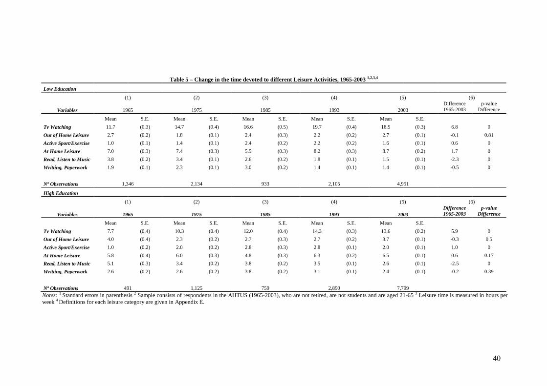
40

Table 5 – Change in the time devoted to different Leisure Activities, 1965-2003 1,2,3,4

Low Education

(1) (2) (3) (4) (5) (6)

Variables 1965 1975 1985 1993 2003

Difference 1965-2003

p-value Difference

Mean S.E. Mean S.E. Mean S.E. Mean S.E. Mean S.E.

Tv Watching 11.7 (0.3) 14.7 (0.4) 16.6 (0.5) 19.7 (0.4) 18.5 (0.3) 6.8 0

Out of Home Leisure 2.7 (0.2) 1.8 (0.1) 2.4 (0.3) 2.2 (0.2) 2.7 (0.1) -0.1 0.81

Active Sport/Exercise 1.0 (0.1) 1.4 (0.1) 2.4 (0.2) 2.2 (0.2) 1.6 (0.1) 0.6 0

At Home Leisure 7.0 (0.3) 7.4 (0.3) 5.5 (0.3) 8.2 (0.3) 8.7 (0.2) 1.7 0

Read, Listen to Music 3.8 (0.2) 3.4 (0.1) 2.6 (0.2) 1.8 (0.1) 1.5 (0.1) -2.3 0

Writting, Paperwork 1.9 (0.1) 2.3 (0.1) 3.0 (0.2) 1.4 (0.1) 1.4 (0.1) -0.5 0

Nº Observations 1,346 2,134 933 2,105 4,951

High Education

(1) (2) (3) (4) (5) (6)

Variables 1965 1975 1985 1993 2003

Difference

1965-2003

p-value

Difference

Mean S.E. Mean S.E. Mean S.E. Mean S.E. Mean S.E.

Tv Watching 7.7 (0.4) 10.3 (0.4) 12.0 (0.4) 14.3 (0.3) 13.6 (0.2) 5.9 0

Out of Home Leisure 4.0 (0.4) 2.3 (0.2) 2.7 (0.3) 2.7 (0.2) 3.7 (0.1) -0.3 0.5

Active Sport/Exercise 1.0 (0.2) 2.0 (0.2) 2.8 (0.3) 2.8 (0.1) 2.0 (0.1) 1.0 0

At Home Leisure 5.8 (0.4) 6.0 (0.3) 4.8 (0.3) 6.3 (0.2) 6.5 (0.1) 0.6 0.17

Read, Listen to Music 5.1 (0.3) 3.4 (0.2) 3.8 (0.2) 3.5 (0.1) 2.6 (0.1) -2.5 0

Writting, Paperwork 2.6 (0.2) 2.6 (0.2) 3.8 (0.2) 3.1 (0.1) 2.4 (0.1) -0.2 0.39

Nº Observations 491 1,125 759 2,890 7,799

Notes: 1 Standard errors in parenthesis 2 Sample consists of respondents in the AHTUS (1965-2003), who are not retired, are not students and are aged 21-65 3 Leisure time is measured in hours per

week 4 Definitions for each leisure category are given in Appendix E.

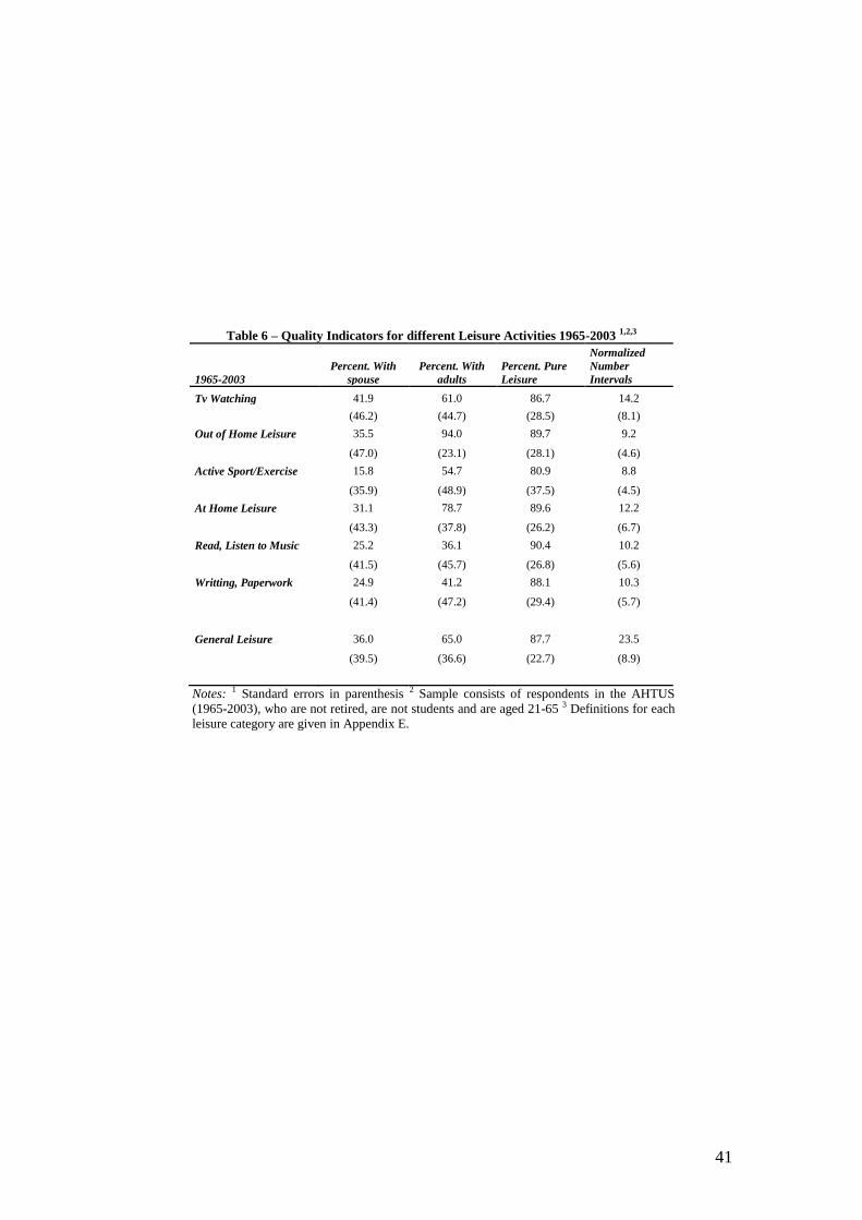
41

Table 6 – Quality Indicators for different Leisure Activities 1965-2003 1,2,3

1965-2003

Percent. With

spouse

Percent. With

adults

Percent. Pure

Leisure

Normalized

Number

Intervals

Tv Watching 41.9 61.0 86.7 14.2

(46.2) (44.7) (28.5) (8.1)

Out of Home Leisure 35.5 94.0 89.7 9.2

(47.0) (23.1) (28.1) (4.6)

Active Sport/Exercise 15.8 54.7 80.9 8.8

(35.9) (48.9) (37.5) (4.5)

At Home Leisure 31.1 78.7 89.6 12.2

(43.3) (37.8) (26.2) (6.7)

Read, Listen to Music 25.2 36.1 90.4 10.2

(41.5) (45.7) (26.8) (5.6)

Writting, Paperwork 24.9 41.2 88.1 10.3

(41.4) (47.2) (29.4) (5.7)

General Leisure 36.0 65.0 87.7 23.5

(39.5) (36.6) (22.7) (8.9)

Notes: 1 Standard errors in parenthesis 2 Sample consists of respondents in the AHTUS

(1965-2003), who are not retired, are not students and are aged 21-65 3 Definitions for each

leisure category are given in Appendix E.

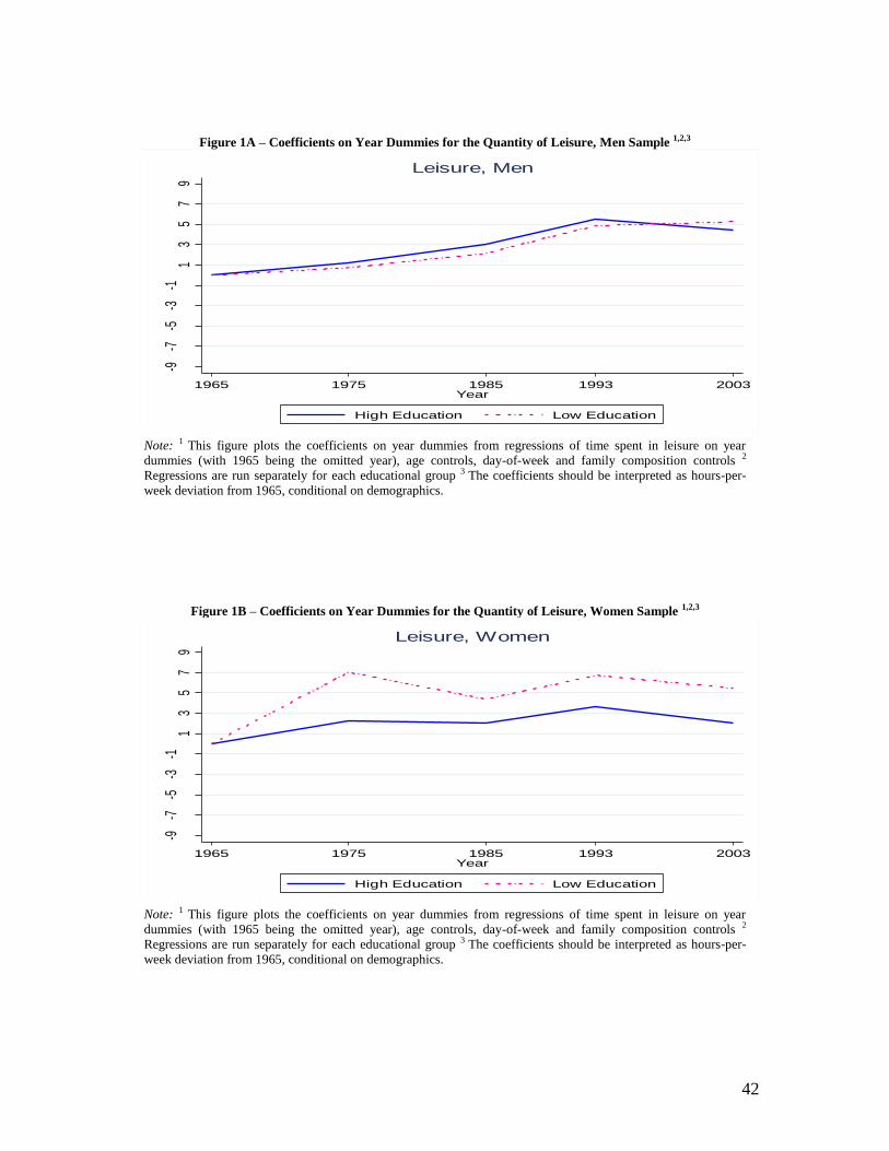
42

Figure 1A – Coefficients on Year Dummies for the Quantity of Leisure, Men Sample 1,2,3

-9-7

-5-3

-11

35

79

Hou

rs p

er w

eek

1965 1975 1985 1993 2003Year

High Education Low Education

Leisure, Men

Note: 1 This figure plots the coefficients on year dummies from regressions of time spent in leisure on year

dummies (with 1965 being the omitted year), age controls, day-of-week and family composition controls 2

Regressions are run separately for each educational group 3 The coefficients should be interpreted as hours-per-

week deviation from 1965, conditional on demographics.

Figure 1B – Coefficients on Year Dummies for the Quantity of Leisure, Women Sample 1,2,3

-9-7

-5-3

-11

35

79

Hou

rs p

er W

eek

1965 1975 1985 1993 2003Year

High Education Low Education

Leisure, Women

Note: 1 This figure plots the coefficients on year dummies from regressions of time spent in leisure on year

dummies (with 1965 being the omitted year), age controls, day-of-week and family composition controls 2

Regressions are run separately for each educational group 3 The coefficients should be interpreted as hours-per-

week deviation from 1965, conditional on demographics.

43

Figure 2A – Coefficients on Year Dummies for the Percentage of Pure Leisure, Men Sample 1,2,3

-9-7

-5-3

-11

35

79

Perc

enta

ge

1965 1975 1985Year

High Education Low Education

Primary Leisure, Men

Note: 1 This figure plots the coefficients on year dummies from regressions of percentage of Pure Leisure on year

dummies (with 1965 being the omitted year), age controls, day-of-week and family composition controls 2

Regressions are run separately for each educational group 3 The coefficients should be interpreted as percentage-

of-Pure-Leisure deviation from 1965, conditional on demographics.

Figure 2B – Coefficients on Year Dummies for the Percentage of Pure Leisure, Women Sample 1,2,3

-9-7

-5-3

-11

35

79

Perc

enta

ge

1965 1975 1985Year

High Education Low Education

Primary Leisure, Women

Note: 1 This figure plots the coefficients on year dummies from regressions of percentage of Pure Leisure on year

dummies (with 1965 being the omitted year), age controls, day-of-week and family composition controls 2

Regressions are run separately for each educational group 3 The coefficients should be interpreted as percentage-

of-Pure-Leisure deviation from 1965, conditional on demographics.

44

Figure 3A – Coefficients on Year Dummies for the Percentage of Leisure with Spouse, Married Men Sample 1,2,3

-9-7

-5-3

-11

35

79

Perc

enta

ge

1965 1975 2003Year

High Education Low Education

Leisure with Spouse, Men

Note: 1 This figure plots the coefficients on year dummies from regressions of percentage of Leisure with Spouse

on year dummies (with 1965 being the omitted year), age controls, day-of-week and family composition controls 2

Regressions are run separately for each educational group for those individuals who are married 3 The coefficients

should be interpreted as percentage-of-Leisure-with-Spouse deviation from 1965, conditional on demographics.

Figure 3B–Coefficients on Year Dummies for the Percentage of Leisure with Spouse, Married Women Sample1,2,3

-9-7

-5-3

-11

35

79

Perc

enta

ge

1965 1975 2003Year

High Education Low Education

Leisure with Spouse, Women

Note: 1 This figure plots the coefficients on year dummies from regressions of percentage of Leisure with Spouse

on year dummies (with 1965 being the omitted year), age controls, day-of-week and family composition controls 2

Regressions are run separately for each educational group for those individuals who are married 3 The coefficients

should be interpreted as percentage-of-Leisure-with-Spouse deviation from 1965, conditional on demographics.

45

Figure 4A – Coefficients on Year Dummies for the Percentage of Leisure with Adults, Men Sample 1,2,3 -9

-7-5

-3-1

13

57

9

Perc

enta

ge

1965 1975 2003Year

High Education Low Education

Leisure with Adults, Men

Note: 1 This figure plots the coefficients on year dummies from regressions of percentage of Leisure with Adults

on year dummies (with 1965 being the omitted year), age controls, day-of-week and family composition controls 2

Regressions are run separately for each educational group 3 The coefficients should be interpreted as percentage-

of-Leisure-with-Adults deviation from 1965, conditional on demographics.

Figure 4B – Coefficients on Year Dummies for the Percentage of Leisure with Adults, Women Sample 1,2,3

-9-7

-5-3

-11

35

79

Perc

enta

ge

1965 1975 2003Year

High Education Low Education

Leisure with Adults, Women

Note: 1 This figure plots the coefficients on year dummies from regressions of percentage of Leisure with Adults

on year dummies (with 1965 being the omitted year), age controls, day-of-week and family composition controls 2

Regressions are run separately for each educational group 3 The coefficients should be interpreted as percentage-

of-Leisure-with-Adults deviation from 1965, conditional on demographics.

46

Figure 5A – Coefficients on Year Dummies for the Number of Leisure Intervals, Men Sample 1,2,3 -1

13

5

Nor

mal

ized

Num

ber

1965 1975 1985 1993 2003Year

High Education Low Education

Leisure Intervals, Men

Note: 1 This figure plots the coefficients on year dummies from regressions of the normalized number of leisure

intervals on year dummies (with 1965 being the omitted year), age controls, day-of-week and family composition

controls 2 Regressions are run separately for each educational group 3 The coefficients should be interpreted as

normalized-number-of-leisure-intervals deviation from 1965, conditional on demographics.

Figure 5B – Coefficients on Year Dummies for the Number of Leisure Intervals, Women Sample 1,2,3

-11

35

Nor

mal

ized

Num

ber

1965 1975 1985 1993 2003Year

High Education Low Education

Leisure Intervals, Women

Note: 1 This figure plots the coefficients on year dummies from regressions of normalized number of leisure

intervals on year dummies (with 1965 being the omitted year), age controls, day-of-week and family composition

controls 2 Regressions are run separately for each educational group 3 The coefficients should be interpreted as

normalized-number-of-leisure-intervals deviation from 1965, conditional on demographics.

47

Figure 6A – Coefficients on Year Dummies for the Fragmentation of Leisure, Men Sample 1,2,3

-6-4

-20

24

6

Perc

enta

ge

1965 1975 1985 1993 2003Year

High Education Low Education

Leisure Poverty, Men

Note: 1 This figure plots the coefficients on year dummies from a linear probability model where the dependent

variable is a dummy that takes value one if the average duration of leisure intervals for a given individual is below

half the median duration of all the intervals in the survey-year of the respondent. The control variables are year

dummies (with 1965 being the omitted year), age controls, day-of-week and family composition controls 2

Regressions are run separately for each educational group 3 The coefficients should be interpreted as the

probability of falling below the a poverty line in the duration of leisure intervals with respect to 1965 conditional

on demographics. This poverty line is defined as half the median duration of all intervals in a given survey-year.

Figure 6B – Coefficients on Year Dummies for the Fragmentation of Leisure, Women Sample1,2,3

-6-4

-20

24

6

Perc

enta

ge

1965 1975 1985 1993 2003Year

High Education Low Education

Leisure Poverty, Women

Note: 1 This figure plots the coefficients on year dummies from a linear probability model where the dependent

variable is a dummy that takes value one if the average duration of leisure intervals for a given individual is below

half the median duration of all the intervals in the survey-year of the respondent. The control variables are year

dummies (with 1965 being the omitted year), age controls, day-of-week and family composition controls 2

Regressions are run separately for each educational group 3 The coefficients should be interpreted as the

probability of falling below the a poverty line in the duration of leisure intervals with respect to 1965 conditional

on demographics. This poverty line is defined as half the median duration of all intervals in a given survey-year.

48

Figure 7A – Coefficients on Year Dummies for the Quantity of Leisure, Working Women 1,2,3

-9-7

-5-3

-11

35

79

Hou

rs p

er W

eek

1965 1975 1985 1993 2003Year

High Education Low Education

Leisure, Working Women

Note: 1 This figure plots the coefficients on year dummies from regressions of time spent in leisure on year

dummies (with 1965 being the omitted year), age controls, day-of-week and family composition controls 2

Regressions are run separately for each educational group 3 The coefficients should be interpreted as hours-per-

week deviation from 1965, conditional on demographics.

Figure 7B – Coefficients on Year Dummies for the Percentage of Pure Leisure, Working Women 1,2,3

-9-7

-5-3

-11

35

79

Perc

enta

ge

1965 1975 1985Year

High Education Low Education

Primary Leisure, Working Women

Note: 1 This figure plots the coefficients on year dummies from regressions of percentage of Pure Leisure on year

dummies (with 1965 being the omitted year), age controls, day-of-week and family composition controls 2

Regressions are run separately for each educational group 3 The coefficients should be interpreted as percentage-

of-Pure-Leisure deviation from 1965, conditional on demographics.

49

Figure 7C – Coefficients on Year Dummies for the Percentage of Leisure with Spouse, Working Women 1,2,3 -9

-7-5

-3-1

13

57

9

Perc

enta

ge

1965 1975 2003Year

High Education Low Education

Leisure with Spouse, Working Women

Note: 1 This figure plots the coefficients on year dummies from regressions of percentage of Leisure with Spouse

on year dummies (with 1965 being the omitted year), age controls, day-of-week and family composition controls 2

Regressions are run separately for each educational group 3 The coefficients should be interpreted as percentage-

of-Leisure-with-Spouse deviation from 1965, conditional on demographics.

Figure 7D – Coefficients on Year Dummies for the Percentage of Leisure with Adults, Working Women 1,2,3

-9-7

-5-3

-11

35

79

Perc

enta

ge

1965 1975 2003Year

High Education Low Education

Leisure with Adults, Working Women

Note: 1 This figure plots the coefficients on year dummies from regressions of percentage of Leisure with Adults

on year dummies (with 1965 being the omitted year), age controls, day-of-week and family composition controls 2

Regressions are run separately for each educational group 3 The coefficients should be interpreted as percentage-

of-Leisure-with-Adults deviation from 1965, conditional on demographics.

50

Figure 7E – Coefficients on Year Dummies for the Number of Leisure Intervals, Working Women 1,2,3

-.05

-.03

-.01

.01

.03

.05

Nor

mal

ized

Num

ber

1965 1975 1985 1993 2003Year

High Education Low Education

Leisure Intervals, Working Women

Note: 1 This figure plots the coefficients on year dummies from regressions of normalized number of leisure

intervals on year dummies (with 1965 being the omitted year), age controls, day-of-week and family composition

controls 2 Regressions are run separately for each educational group 3 The coefficients should be interpreted as

normalized-number-of-leisure-intervals deviation from 1965, conditional on demographics.

Figure 7F – Coefficients on Year Dummies for the Fragmentation of Leisure, Working Women 1,2,3

-6-4

-20

24

6

Perc

enta

ge

1965 1975 1985 1993 2003Year

High Education Low Education

Leisure Poverty, Working Women

Note: 1 This figure plots the coefficients on year dummies from a linear probability model where the dependent

variable is a dummy that takes value one if the average duration of leisure intervals for a given individual is below

half the median duration of all the intervals in the survey-year of the respondent. The control variables are year

dummies (with 1965 being the omitted year), age controls, day-of-week and family composition controls 2

Regressions are run separately for each educational group 3 The coefficients should be interpreted as the

probability of falling below the a poverty line in the duration of leisure intervals with respect to 1965 conditional

on demographics. This poverty line is defined as half the median duration of all intervals in a given survey-year.

51

Figure 8A – Coefficients on Year Dummies for the Quantity of Leisure, Men Sample

(without TV Watching)1,2,3

-4-2

02

4

Hou

rs p

er w

eek

1965 1975 1985 1993 2003Year

High Education Low Education

Leisure, Men

Note: 1 This figure plots the coefficients on year dummies from regressions of time spent in leisure on year

dummies (with 1965 being the omitted year), age controls, day-of-week and family composition controls 2

Regressions are run separately for each educational group 3 The coefficients should be interpreted as hours-per-

week deviation from 1965, conditional on demographics 4 The definition of leisure does not include Watching

Television.

Figure 8B – Coefficients on Year Dummies for the Quantity of Leisure, Women Sample

(without TV Watching) 1,2,3

-4-2

02

4

Hou

rs p

er W

eek

1965 1975 1985 1993 2003Year

High Education Low Education

Leisure, Women

Note: 1 This figure plots the coefficients on year dummies from regressions of time spent in leisure on year

dummies (with 1965 being the omitted year), age controls, day-of-week and family composition controls 2

Regressions are run separately for each educational group 3 The coefficients should be interpreted as hours-per-

week deviation from 1965, conditional on demographics 4 The definition of leisure does not include Watching

Television.

52

Figure 9A – Coefficients on Year Dummies for the Percentage of Pure Leisure, Men Sample

(without TV Watching)1,2,3

-8-6

-4-2

02

46

810

1214

16

Perc

enta

ge

1965 1975 1985Year

High Education Low Education

Primary Leisure, Men

Note: 1 This figure plots the coefficients on year dummies from regressions of percentage of Pure Leisure on year

dummies (with 1965 being the omitted year), age controls, day-of-week and family composition controls 2

Regressions are run separately for each educational group 3 The coefficients should be interpreted as percentage-

of-Pure-Leisure deviation from 1965, conditional on demographics 4 The definition of leisure does not include

Watching Television.

Figure 9B – Coefficients on Year Dummies for the Percentage of Pure Leisure, Women Sample

(without TV Watching)1,2,3

-8-6

-4-2

02

46

810

1214

16

Perc

enta

ge

1965 1975 1985Year

High Education Low Education

Primary Leisure, Women

Note: 1 This figure plots the coefficients on year dummies from regressions of percentage of Pure Leisure on year

dummies (with 1965 being the omitted year), age controls, day-of-week and family composition controls 2

Regressions are run separately for each educational group 3 The coefficients should be interpreted as percentage-

of-Pure-Leisure deviation from 1965, conditional on demographics 4 The definition of leisure does not include

Watching Television.

53

Figure 10A – Coefficients on Year Dummies for the Percentage of Leisure with Spouse, Married Men Sample

(without TV Watching)1,2,3 -9

-7-5

-3-1

13

57

9

Perc

enta

ge

1965 1975 2003Year

High Education Low Education

Leisure with Spouse, Men

Note: 1 This figure plots the coefficients on year dummies from regressions of percentage of Leisure with Spouse

on year dummies (with 1965 being the omitted year), age controls, day-of-week and family composition controls 2

Regressions are run separately for each educational group for those individuals who are married 3 The coefficients

should be interpreted as percentage-of-Leisure-with-Spouse deviation from 1965, conditional on demographics 4

The definition of leisure does not include Watching Television.

Figure 10B–Coefficients on Year Dummies for the Percentage of Leisure with Spouse, Married Women Sample

(without TV Watching)1,2,3

-9-7

-5-3

-11

35

79

Perc

enta

ge

1965 1975 2003Year

High Education Low Education

Leisure with Spouse, Women

Note: 1 This figure plots the coefficients on year dummies from regressions of percentage of Leisure with Spouse

on year dummies (with 1965 being the omitted year), age controls, day-of-week and family composition controls 2

Regressions are run separately for each educational group for those individuals who are married 3 The coefficients

should be interpreted as percentage-of-Leisure-with-Spouse deviation from 1965, conditional on demographics 4

The definition of leisure does not include Watching Television.

54

Figure 11A – Coefficients on Year Dummies for the Percentage of Leisure with Adults, Men Sample

(without TV Watching) 1,2,3 -7

-5-3

-11

35

7

Perc

enta

ge

1965 1975 2003Year

High Education Low Education

Leisure with Adults, Men

Note: 1 This figure plots the coefficients on year dummies from regressions of percentage of Leisure with Adults

on year dummies (with 1965 being the omitted year), age controls, day-of-week and family composition controls 2

Regressions are run separately for each educational group 3 The coefficients should be interpreted as percentage-

of-Leisure-with-Adults deviation from 1965, conditional on demographics 4 The definition of leisure does not

include Watching Television.

Figure 11B – Coefficients on Year Dummies for the Percentage of Leisure with Adults, Women Sample

(without TV Watching)1,2,3

-7-5

-3-1

13

57

Perc

enta

ge

1965 1975 2003Year

High Education Low Education

Leisure with Adults, Women

Note: 1 This figure plots the coefficients on year dummies from regressions of percentage of Leisure with Adults

on year dummies (with 1965 being the omitted year), age controls, day-of-week and family composition controls 2

Regressions are run separately for each educational group 3 The coefficients should be interpreted as percentage-

of-Leisure-with-Adults deviation from 1965, conditional on demographics 4 The definition of leisure does not

include Watching Television.

55

Figure 12A – Coefficients on Year Dummies for the Number of Leisure Intervals, Men Sample

(without TV Watching)1,2,3 -5

-3-1

13

5

Nor

mal

ized

Num

ber

1965 1975 1985 1993 2003Year

High Education Low Education

Leisure Intervals, Men

Note: 1 This figure plots the coefficients on year dummies from regressions of the normalized number of leisure

intervals on year dummies (with 1965 being the omitted year), age controls, day-of-week and family composition

controls 2 Regressions are run separately for each educational group 3 The coefficients should be interpreted as

normalized-number-of-leisure-intervals deviation from 1965, conditional on demographics 4 The definition of

leisure does not include Watching Television.

Figure 12B – Coefficients on Year Dummies for the Number of Leisure Intervals, Women Sample

(without TV Watching)1,2,3

-5-3

-11

35

Nor

mal

ized

Num

ber

1965 1975 1985 1993 2003Year

High Education Low Education

Leisure Intervals, Women

Note: 1 This figure plots the coefficients on year dummies from regressions of normalized number of leisure

intervals on year dummies (with 1965 being the omitted year), age controls, day-of-week and family composition

controls 2 Regressions are run separately for each educational group 3 The coefficients should be interpreted as

normalized-number-of-leisure-intervals deviation from 1965, conditional on demographics 4 The definition of

leisure does not include Watching Television.

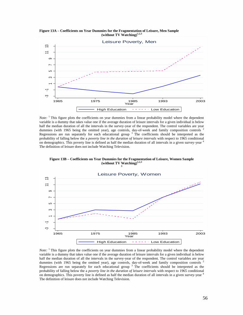
56

Figure 13A – Coefficients on Year Dummies for the Fragmentation of Leisure, Men Sample

(without TV Watching)1,2,3

-3-1

13

57

911

13

Perc

enta

ge

1965 1975 1985 1993 2003Year

High Education Low Education

Leisure Poverty, Men

Note: 1 This figure plots the coefficients on year dummies from a linear probability model where the dependent

variable is a dummy that takes value one if the average duration of leisure intervals for a given individual is below

half the median duration of all the intervals in the survey-year of the respondent. The control variables are year

dummies (with 1965 being the omitted year), age controls, day-of-week and family composition controls 2

Regressions are run separately for each educational group 3 The coefficients should be interpreted as the

probability of falling below the a poverty line in the duration of leisure intervals with respect to 1965 conditional

on demographics. This poverty line is defined as half the median duration of all intervals in a given survey-year 4

The definition of leisure does not include Watching Television.

Figure 13B – Coefficients on Year Dummies for the Fragmentation of Leisure, Women Sample

(without TV Watching)1,2,3 3

-3-1

13

57

911

13

Perc

enta

ge

1965 1975 1985 1993 2003Year

High Education Low Education

Leisure Poverty, Women

Note: 1 This figure plots the coefficients on year dummies from a linear probability model where the dependent

variable is a dummy that takes value one if the average duration of leisure intervals for a given individual is below

half the median duration of all the intervals in the survey-year of the respondent. The control variables are year

dummies (with 1965 being the omitted year), age controls, day-of-week and family composition controls 2

Regressions are run separately for each educational group 3 The coefficients should be interpreted as the

probability of falling below the a poverty line in the duration of leisure intervals with respect to 1965 conditional

on demographics. This poverty line is defined as half the median duration of all intervals in a given survey-year 4

The definition of leisure does not include Watching Television.

57

APPENDIX A

Appendix A Table A1: AHTUS Description 1

Study aims, target populations, and sample restrictions

Survey years Organizing Aims and Considerations Target Population Sampling Restrictions

1965-1966 Comparability with the Multinational Comparative Time-Budget project collected in 12 countries

The national working age population (19-64) of the USA

(excluding families where all

members worked as farmers)

Only people aged 19 to 64 (with a few older diarists), and one person per household

(Alaska, Hawaii, and some smaller, rural

states excluded)

1975-1976 Measure national accounts and changes in time use over

the year

The national adult population People aged 18 or older and one person plus

spouse if present per household

1985 Determined how people used their time and to compare

diaries collected by post-out/post-back, phone, and face-to-face interview

The national population beyond

secondary school age not living in institutions

People aged 12 or older living in private

households with phones (Alaska, Hawaii, and some smaller, rural states excluded)

1992-1994 The study measured time use and exposure The national population living in

private residences

1 person of any age living in sampled

private households with phones (Alaska and

Hawaii excluded)

2003 The study follows a sub-sample of the CPS for a 9th

wave to facilitate the study of national accounts

The national population not living

in military bases or institutions

1 person aged 15 or older in the household

Relevant points in time from the sample designs

Survey years Fieldwork Period Sampling of Days of the Week When Activities Were Recorded

1965-1966 15 November -15 December 1965;

1 January - 18 February 1966; 7 March - 20 May, 1966

2/7ths of diaries were stamped for

collection on a weekend day; 5/7ths

were stamped for collection on a weekday

A two-stage tomorrow approach, diaries

left behind for completion on diary day

1975-1976 Wave 1: 9 October 1975 – 22 November 1975; Wave 2: 6 February 1976 - 28 March 1976; Wave 3: 2 May 1976

- 19 July 1976; Wave 4: 4 September 1976 - 26 October

1976

The study aimed to collect one diary on a Sunday, one on a Saturday, and

two on different weekdays from

each sample member.

Diaries covered the previous 24 hour day

1985 Whole year of 1985 Mail-out after phone calls. Diaries to be completed on a specified day

in the subsequent week

1992-1994 September 1992 – October 1994 Phone calls were attempted on all

days of the week.

Diaries covered the previous 24 hour day

2003 Whole year of 2003 Half of diaries were collected on weekday, half on weekend days.

Diaries covered the previous 24 hour day

Sample designs and response rates

Survey years Sample Frame How Sample Drawn Response Rate

1965-1966 Jackson, Michigan and surrounding townships, and a national sample

Jackson – random selection; National multi-stage clustered area

sampling of clusters containing

around 4 addresses; one individual per household

82 per cent in Jackson; 74 per cent in the national sample

1975-1976 Private households Stratified, clustered and probability

selection within strata. One individual was sampled per

household. Data was also collected

from spouses where present.

72 per cent in the first wave; 44.9 per cent

responded to all four waves

1985 Adults 18 years or over, living in houses with telephones

in the contiguous United States.

Stratified and clustered, random-

digit dialing, with only private

residences pursued for an interview.

Information on the household collected by telephone.

55.2 per cent overall, 51 per cent for mail

back sample

1992-1994 Potential phone numbers within lists of area codes Random-digit dialing, only private

residences pursued for interview. The person who would net have a

birthday completed the diary.

63 per cent

2003 The CPS sample A random sub-sample of the CPS, with the over-sampling of small

states dropped but families with

children over-sampled. Half of the diaries are collected on week days,

the other half on weekend days

57.8 per cent

Note: 1 Source: Fisher et al [2006].

58

Appendix A Table A2: AHTUS Codes and Leisure Codes 1,2

1965 1975-76 1985 1992-94 2003

-8 item missing

1 general or other personal care

2 imputed personal or household care

3 Sleep

4 imputed sleep

5 naps and rest N/A

6 wash, dress, personal care

7 personal medical care

8 meals at work N/A

9 other meals & snacks

10 main paid work (not at home)

11 paid work at home

12 Second job, other paid work

13 work breaks

14 other time at workplace N/A

15 time looking for work N/A

16 regular schooling, education

17 Homework

18 short course or training

19 occasional or other education/training

20 food preparation, cooking

21 set table, wash/put away dishes

22 Cleaning

23 laundry, ironing, clothing repair

24 home repairs, maintain vehicle

25 other domestic work

26 purchase routine goods

27 purchase consumer durables

28 purchase personal services

29 purchase medical services

30 purchase repair, laundry services

31 financial/government services

32 purchase other services

33 care of infants

34 general care of older children

35 medical care of children

36 play with children

37 supervise child or help with homework

38 read to, talk with child

39 other child care

40 adult care

41 general voluntary acts

42 political and civic activity

43 union and professional activities N/A N/A 44 volunteer child/family organization N/A N/A 45 volunteer fraternal organization N/A N/A 46 other formal volunteering N/A 48 acts for religious organization N/A 49 worship and religious acts

50 general out-of-home leisure L N/A

Notes: 1 N/A indicates that the activity is not available in that particular survey and L indicates that the activity is assumed to be a leisure

activity 2 Source: Fisher et al [2006].

59

Appendix A Table A2 (Cont.). AHTUS Codes and Leisure Codes 1,2

1965 1975-76 1985 1992-94 2003

51 attend sporting event L

52 go to cinema L

53 theater, concert, opera L

54 museums, exhibitions L

55 attend other public event L N/A

56 restaurant, cafe bar L

57 Parties or receptions L

58 imputed time away from home L

60 sports & exercise L

62 Walking L N/A

63 Cycling L N/A N/A

64 outdoor recreation L N/A

65 physical activity, sports with child L

66 hunting, fishing, boating, hiking L N/A

67 Gardening N/A

68 pet care, walk dogs N/A

70 general indoor leisure L

71 imputed in-home social L

72 receive or visit friends L

73 other in-home social, games L

74 play musical instrument, sing, act L N/A

75 Artistic activity L N/A

76 Crafts L N/A

77 Hobbies L

78 relax, think, do nothing L

81 read books L

82 read periodicals L N/A

83 read newspapers L N/A

84 Listen to music (CD etc.) L

85 listen to radio L

86 watch television, video L

87 writing by hand L

88 conversation, phone, texting L

89 use computer L N/A N/A

90 imputed travel N/A N/A

91 personal or adult care travel N/A N/A

92 travel as part of paid work N/A N/A N/A

93 travel to/from work + other work travel N/A

94 travel related to education N/A

95 travel related to consumption

96 travel related to child care

97 travel for volunteering or worship

98 other travel

Notes: 1 N/A indicates that the activity is not available in that particular survey and L indicates that the activity is assumed to be a leisure

activity 2 Source: Fisher et al [2006].

60

APPENDIX B

Appendix B Table B1– Variables used in the validation exercise 1,2,3,4

Leisure dilution

primary leisure secondary work D

Leisure fragmentation

mean hours per leisure period C

daily number leisure periods C

Co-present leisure (UK only)

spouse present during activity D

friend present during activity D

Demographic variables

Woman DC

Age C

age squared C

employed full time DC

employed part time DC

has child aged under 5 DC

has child age 5-18 DC

Leisure Activity variables

primary paid or unpaid work D

primary out of home leisure D

primary active sport exercise D

primary read, listen to music D

primary watch television D

primary writing, paperwork etc D

primary sleep or personal D

Notes: 1 Source: AHTUS 1985 and Unilever 1986 2 We select the same age range

from the two samples (18-72, slightly broader than that used elsewhere in this

paper), and consider just those US diarists with co-resident partners 3 The

designation D indicates 0-1 dummy variables; C indicates variable which are

constant across all the events of a particular respondent‘s day 4 Definitions for each

leisure category are given in Appendix E.

61

APPENDIX C

Appendix C Table C1 – Demographic composition of the time-diary samples in AHTUS1,2

Men

(1) (2) (3) (4) (5)

Variables 1965 1975 1985 1993 2003

Mean S.E. Mean S.E. Mean S.E. Mean S.E. Mean S.E.

Age 40.6 (12.3) 39.5 (12.2) 38.7 (11.6) 39.3 (11.2) 41.8 (11.3)

College 0.3 (0.5) 0.4 (0.5) 0.5 (0.5) 0.6 (0.5) 0.6 (0.5)

Married 0.9 (0.3) 0.8 (0.4) 0.7 (0.4) - - 0.7 (0.5)

Presence of

Children 0.6 (0.5) 0.5 (0.5) 0.4 (0.5) 0.3 (0.4) 0.4 (0.5)

Number of

Children 1.5 (1.6) 1.2 (1.4) 0.8 (1.0) 0.5 (1.0) 0.8 (1.1)

Working 1.0 (0.1) 0.9 (0.3) 0.9 (0.2) 0.9 (0.3) 0.9 (0.3)

Nº Observations 854 1,437 830 2,497 6,182

Women

(1) (2) (3) (4) (5)

Variables 1965 1975 1985 1993 2003

Mean S.E. Mean S.E. Mean S.E. Mean S.E. Mean S.E.

Age 41.0 (12.4) 40.1 (12.7) 38.9 (12.1) 39.4 (11.4) 42.1 (11.5)

College 0.2 (0.4) 0.3 (0.4) 0.4 (0.5) 0.6 (0.5) 0.6 (0.5)

Married 0.8 (0.4) 0.7 (0.5) 0.7 (0.5) - - 0.6 (0.5)

Presence of

Children 0.6 (0.5) 0.6 (0.5) 0.4 (0.5) 0.3 (0.5) 0.5 (0.5)

Number of

Children 1.4 (1.6) 1.2 (1.3) 0.7 (1.0) 0.6 (1.0) 0.9 (1.1)

Working 0.5 (0.5) 0.6 (0.5) 0.7 (0.5) 0.8 (0.4) 0.8 (0.4)

Nº Observations 1,048 1,921 914 2,888 7,557

Note: 1 Standard errors in brackets 2 Sample consists of individuals in the AHTUS (1965-2003), who are not retired, are not students and are aged 21-65.

62

APPENDIX D

Appendix D Table D1. Coefficients on Year Dummies, Men Sample 1,2,3

Low Education

(1) (2) (3) (4) (5)

Variables 1975 1985 1993 2003

Number

Observ.

Coeff S.E. Coeff S.E. Coeff S.E. Coeff S.E.

Leisure Time 0.7 (1.1) 2.1* (1.2) 4.9*** (1.1) 5.3*** (0.9) 4,919

Percentage Pure Leisure -3.5** (1.5) -6.3*** (1.8) - - - - 1,820

Percentage Leisure with Spouse -0.8 (2.3) - - - - -13.2*** (1.9) 3,565

Percentage Leisure with Adults -1.7 (1.9) - - - - -10.5*** (1.6) 3,565

Normalized number of Leisure Intervals -0.2 (0.5) 0.7 (0.6) 1.8*** (0.5) 1.6*** (0.4) 4,767

Poverty in the Duration of Leisure Intervals 6.0*** (1.3) 0.2 (1.1) 0.0 (0.0) 4.7*** (1.0) 3,995

High Education

(1) (2) (3) (4) (5)

Variables 1975 1985 1993 2003

Number

Observ.

Coeff S.E. Coeff S.E. Coeff S.E. Coeff S.E.

Leisure Time 1.2 (1.2) 3.1** (1.4) 5.5*** (1.2) 4.4*** (1.1) 6,117

Percentage Pure Leisure -5.7*** (2.0) -3.5* (2.1) - - - - 1,263

Percentage Leisure with Spouse 4.3 (2.9) - - - - -7.4*** (2.5) 4,346

Percentage Leisure with Adults 3.2 (2.7) - - - - -6.8*** (2.3) 4,346

Normalized number of Leisure Intervals -0.7 (0.8) 0.9 (0.8) 1.7** (0.7) 0.6 (0.7) 5,913

Poverty in the Duration of Leisure Intervals 1.5 (2.1) -4.7*** (1.8) 0.0 (0.0) 1.0 (1.7) 4,731

Notes: 1 This table reports the coefficients and standard errors for the time dummies that are plotted in the Figures 2 See notes to the figures for full sample and methodological

descriptions 3 ***Significant at the 1 per cent level **Significant at the 5 per cent level *Significant at the 10 per cent level.

63

Appendix D Table D2. Coefficients on Year Dummies, Women Sample 1,2,3

Low Education

(1) (2) (3) (4) (5)

Variables 1975 1985 1993 2003 Number Observ.

Coeff S.E. Coeff S.E. Coeff S.E. Coeff S.E.

Leisure Time 7.0*** (0.8) 4.4*** (1.0) 6.7*** (0.9) 5.5*** (0.8) 6,545

Percentage Pure Leisure -1.6 (1.2) -6.8*** (1.6) - - - - 2,677

Percentage Leisure with Spouse -2.9* (1.7) - - - - -5.6*** (1.5) 4,861

Percentage Leisure with Adults 1.0 (1.5) - - - - -4.7*** (1.5) 4,861

Normalized number of Leisure Intervals 2.7*** (0.4) 2.5*** (0.5) 3.6*** (0.4) 4.0*** (0.4) 6,352

Poverty in the Duration of Leisure Intervals 1.9* (1.0) -1.3 (1.0) 0.0 (0.0) 5.8*** (1.0) 5,384

High Education

(1) (2) (3) (4) (5)

Variables 1975 1985 1993 2003 Number Observ.

Coeff S.E. Coeff S.E. Coeff S.E. Coeff S.E.

Leisure Time 2.2* (1.3) 2.0 (1.3) 3.6*** (1.2) 2.1** (1.1) 7,142

Percentage Pure Leisure -2.6 (2.0) -4.4** (2.0) - - - - 1,165

Percentage Leisure with Spouse 2.5 (2.9) - - - - -0.7 (2.4) 5,204

Percentage Leisure with Adults -0.2 (2.7) - - - - -4.9** (2.2) 5,204

Normalized number of Leisure Intervals 1.9*** (0.6) 2.3*** (0.7) 3.6*** (0.6) 3.3*** (0.5) 6,904

Poverty in the Duration of Leisure Intervals 4.5** (1.9) 2.2 (1.8) 0.0 (0.0) 6.9*** (1.4) 5,588

Notes: 1 This table reports the coefficients and standard errors for the time dummies that are plotted in the Figures 2 See notes to the figures for full sample and methodological

descriptions 3 ***Significant at the 1 per cent level **Significant at the 5 per cent level *Significant at the 10 per cent level.

64

Appendix D Table D3 Coefficients on Year Dummies, Working Women 1,2,3

Low Education

(1) (2) (3) (4) (5)

Variables 1975 1985 1993 2003

Number

Observ.

Coeff S.E. Coeff S.E. Coeff S.E. Coeff S.E.

Leisure Time 6.8*** (1.0) 5.5*** (1.2) 7.7*** (1.1) 7.0*** (0.9) 4,017

Percentage Pure Leisure 1.8 (1.8) -7.7*** (2.3) - - - - 1,426

Percentage Leisure with Spouse 4.4* (2.5) - - - - 3.3 (2.2) 2,892

Percentage Leisure with Adults 5.5** (2.5) - - - - -1.1 (2.3) 2,892

Normalized number of Leisure Intervals 2.3*** (0.5) 2.7*** (0.6) 4.0*** (0.6) 4.4*** (0.5) 3,860

Poverty in the Duration of Leisure Intervals 0.9 (1.5) -1.9 (1.5) 0.0 (0.0) 7.3*** (1.5) 3,238

High Education

(1) (2) (3) (4) (5)

Variables 1975 1985 1993 2003

Number

Observ.

Coeff S.E. Coeff S.E. Coeff S.E. Coeff S.E.

Leisure Time 4.0*** (1.5) 4.9*** (1.5) 6.5*** (1.3) 5.0*** (1.2) 5,612

Percentage Pure Leisure -1.4 (3.3) -1.0 (3.0) - - - - 740

Percentage Leisure with Spouse 3.9 (3.9) - - - - 5.6* (3.3) 4,006

Percentage Leisure with Adults -1.1 (3.9) - - - - -3.4 (3.3) 4,006

Normalized number of Leisure Intervals 2.4*** (0.8) 3.3*** (0.8) 4.7*** (0.7) 4.6*** (0.7) 5,394

Poverty in the Duration of Leisure Intervals 4.0 (2.7) 0.8 (2.5) 0.0 (0.0) 6.0*** (2.1) 4,298

Notes: 1 This table reports the coefficients and standard errors for the time dummies that are plotted in the Figures 2 See notes to the figures for full sample and methodological

descriptions 3 ***Significant at the 1 per cent level **Significant at the 5 per cent level *Significant at the 10 per cent level.

65

APPENDIX E

The leisure activities included in each of the leisure categories in Section 4 and in Table 6 are

the following:

―TV Watching‖ includes the time devoted to ―TV Watching‖.

―Out of Home Leisure‖ includes the time devoted to "general out-of-home leisure", "attend

sporting event", "go to cinema", "theater, concert, opera", museums, exhibitions", "attend other

public event", "restaurant, cafe bar", "Parties or receptions", "imputed time away from home".

―Active Sport Exercise‖ includes the time devoted to "sports and exercise", "Walking",

"Cycling", "outdoor recreation", "physical activity, sports with child", "hunting, fishing, boating,

hiking".

―At-Home Leisure‖ includes the time devoted to "general indoor leisure", "imputed in-home

social", "receive or visit friends", "other in-home social, games", "play musical instrument, sing,

act", "Artistic activity", "Crafts", "Hobbies", "relax, think, do nothing".

―Read/Listen‖ includes the time devoted to "read books", "read periodicals", "read

newspapers", "Listen to music (CD etc.)", "listen to radio".

―Writing, paperwork…‖ includes the time devoted to "writing by hand", "conversation,

phone, ―texting", use computer.