Social Automata• Agent-based models

– Contrast to global descriptive models– Local interactions by agents

• Assumptions– Agents are autonomous: bottom-up control of system– Agents are interdependent– Agents follow simple rules– Agents adapt, but are not optimal

Schelling’s Segregation Model• Mild preference to be close to others similar to oneself

leads to dramatic segregation– Conflict between local preferences and global solution– Nobody may want a segregated community, but it occurs anyway

• Model– 2-D lattice with Moore neighborhoods– Two types of individuals– If < 37% of neighbors are of an agent’s type, then the agent moves to a

location where at least 37% of its neighbors are of its type

Schelling’s Segregation Model

A perfectly integrated, butimprobable, community

A random starting communitywith some discontent

Schelling’s Segregation Model

A community after several iterations ofdistcontented people moving

Large events are rare, small events common

The population of a city is inversely proportional to its rank

Log (rank of city) = Log (population)-P

P=1

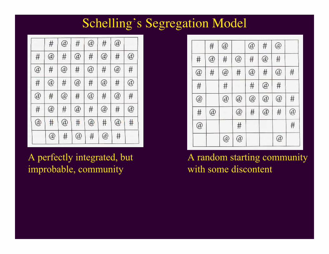
Log (rank of word) = Log (probability)-P

P=1

Situations where log-log linear plots are found• Gutenberg-Richter law

– X: the size of an earthquake, Y: the frequency of the earthquake

• Words (Zipf’s law)– X: rank of a word, Y: frequency of word

• Citations– X: rank of paper in terms of citations, Y: number of citations

• Animal sizes– X: Size of a species (Kg), Y: number of species with this size

Three related laws

Zipf’s Law: the size of the Rth largest occurrence of an event isinversely proportional to its rank

Pareto’s law: probability of having an income greater than x

†

size µ rank-B ,B ª1

†

P(X > x) µ x-k

Power law distribution

†

P(X = x) µ x-(k +1) = x-a

This PDF is the derivative of Pareto’s law’s CDF

Power laws

A mathematical relation that forms linear plots when datais transformed into log-log coordinates

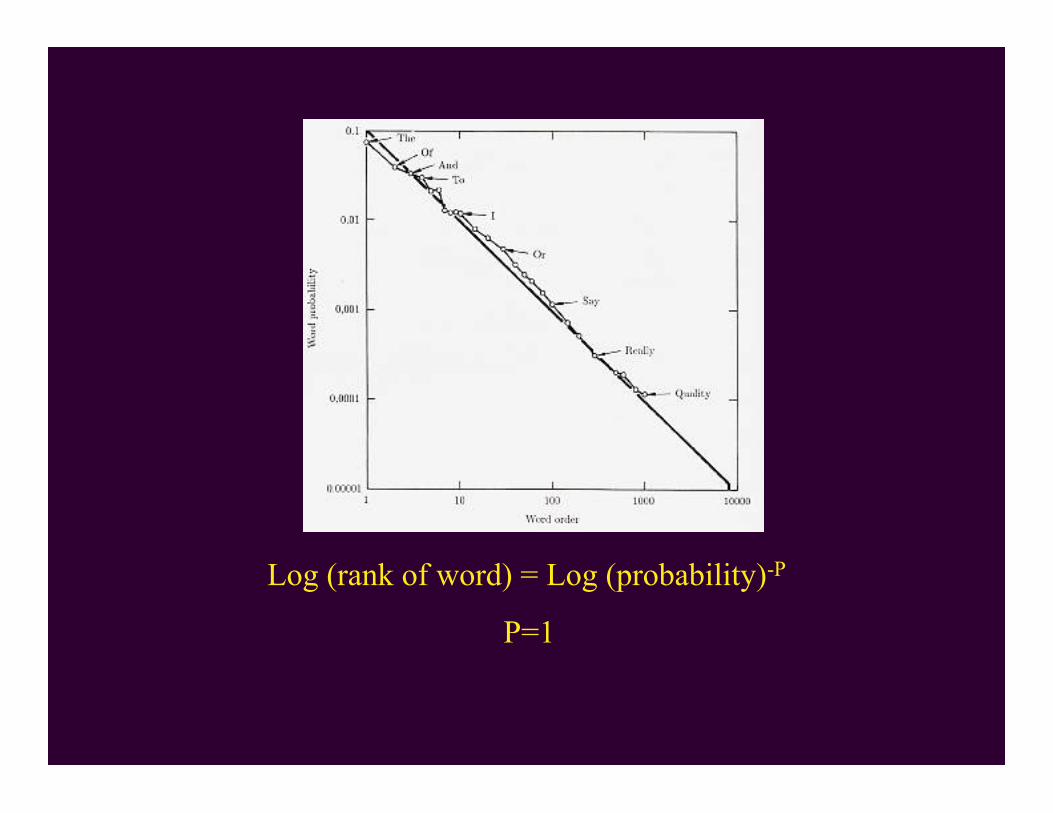
Very few sites have many users

Power laws

A power function with slope =-2.07 fits the AOL data well

P(site has X visitors) = CX-2.07

Zipf’s law

Number of unique visitors is inversely proportional tothe rank of the site

The Rth largest site has N visitors is equivalent to:

R sites have N or more visitors (as in Pareto’s law)

From Zipf’s Law to Power Function

†

size µ rank-B ,B ª1

†

P(X = x) = x-a

†

a =1+1B

†

P X ≥ rank-B( ) = rank There are rank variables withvalues of at least rank-B

†

P X ≥ x( ) = x-

1B Switch variables

†

P X = x( ) = x- 1+

1b

Ê

Ë Á

ˆ

¯ ˜ Take derivative to move from

CDF to PDF

Power Law in Bibliometrics

Ln (citations to Goldstone) = Ln (rank of citation)-1.59

Ln (Rank)3.53.02.52.01.51.0.50.0-.5

7

6

5

4

3

2

1

0

-1

Observed

Y=X^-1.59L

n(ci

tatio

ns)

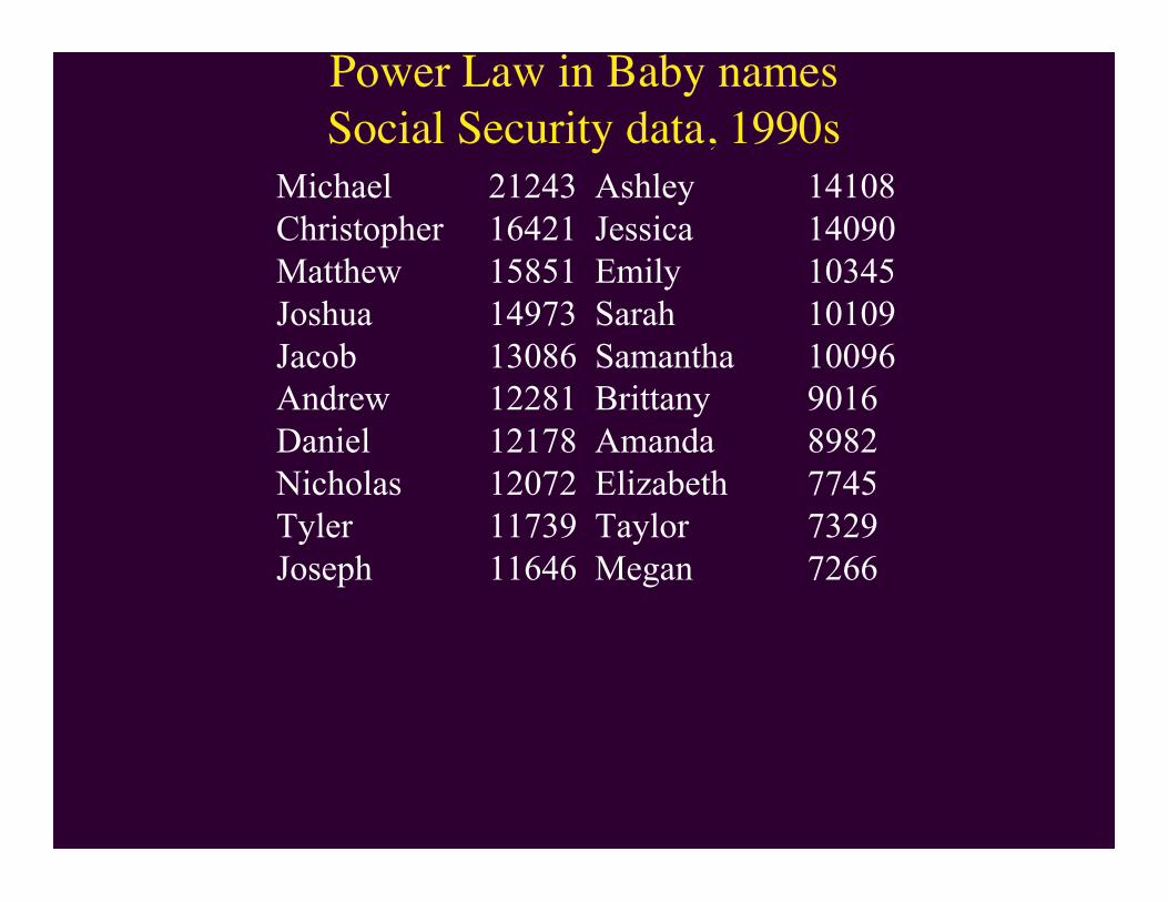
Power Law in Baby namesSocial Security data, 1990s

Michael 21243 Ashley 14108Christopher 16421 Jessica 14090Matthew 15851 Emily 10345Joshua 14973 Sarah 10109Jacob 13086 Samantha 10096Andrew 12281 Brittany 9016Daniel 12178 Amanda 8982Nicholas 12072 Elizabeth 7745Tyler 11739 Taylor 7329Joseph 11646 Megan 7266

Power Law in Baby namesSocial Security data, 1990s

LNGIRL

LNRANK76543210-1

14

12

10

8

6

4ObservedLinear

LNBOY

LNRANK76543210-1

14

12

10

8

6

4

2ObservedLinear

Apparent departure from power law, but only for a verysmall number of most common names. Ln(10) = 2.3, soonly 10 data points out of 100 make up deviation

Power Law in Baby names

RANK120010008006004002000-200

3000

2000

1000

0

ObservedLinearLogari thmicPowerExponentia lLogistic

RANK120010008006004002000-200

3000

2000

1000

0

ObservedLinearLogari thmicPowerExponentia lLogistic

Freq

uenc

y of

Nam

e

Boy names Girl names

Untransformed data (Cutting out the top four names)Power law fits bestBoy exponent = -1.34, Girl exponent = -1.11

Naming for boys is more “elitist” than girls (faster drop-off of frequency with rank)

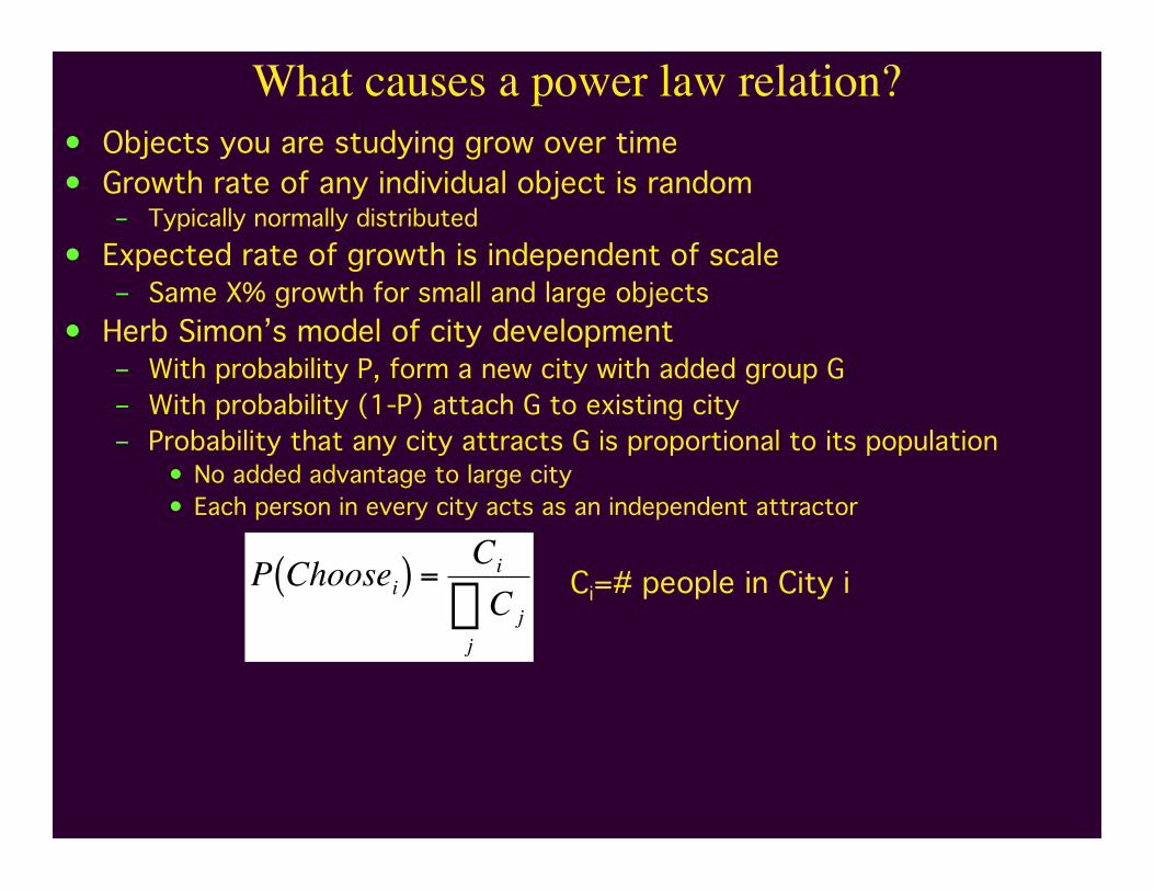
What causes a power law relation?• Objects you are studying grow over time• Growth rate of any individual object is random

– Typically normally distributed• Expected rate of growth is independent of scale

– Same X% growth for small and large objects• Herb Simon’s model of city development

– With probability P, form a new city with added group G– With probability (1-P) attach G to existing city– Probability that any city attracts G is proportional to its population

• No added advantage to large city• Each person in every city acts as an independent attractor

†

P Choosei( ) =Ci

C jj

 Ci=# people in City i

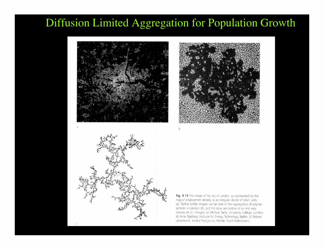
Diffusion Limited Aggregation for Population Growth

Sugarscape (Epstein & Axtell)• Explain social and economic behaviors at large scale through

individual behaviors (bottom-up economics)• Agents

– Vision: high is good– Metabolism: low is good

• Movement: move to cell within vision with greatest sugar• GR: grow sugar back with rate R• Replacement: Replace dead agent with random new agent

Wealth Distribution• Uniform random assignments of vision and metabolism still results

in unequal, pyramidal distribution of wealth• Start simulation with number of agents at the carrying capacity• Random life spans within a range, and death from starvation• Replace dead agent with new agent with random new agent

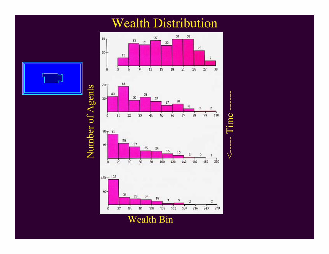
Wealth Distribution

Num

ber

of A

gent

s

Wealth Bin<-

----

Tim

e --

----

Wealth Distribution

<---

-- T

ime

----

--

% of Population

% o

f W

ealth

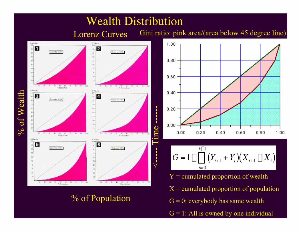
Lorenz Curves Gini ratio: pink area/(area below 45 degree line)

†

G =1- Yi+1 + Yi( )i= 0

k-1

 Xi+1 - Xi( )

Y = cumulated proportion of wealth

X = cumulated proportion of population

G = 0: everybody has same wealth

G = 1: All is owned by one individual

Why an Unequal Distribution of Wealth?• Epstein & Axtell: “Agents having wealth above the mean frequently

have both high vision and low metabolism. In order to become oneof the very wealthiest agents one must also be born high on thesugarscape and live a long life.”

• This is part of the story, but not completely satisfying if vision andmetabolism variables are uniformly or normally distributed

• multiplicative effect of variables?• Binomial and Poisson distributions

– Binomial function describes the probability of obtaining xoccurrences of event A when each of N events is independentof the others, and the probability of event A on any trial is P:

†

F x( ) =N!

x! N - x( )!Px 1- P( )N-x

- Poisson distribution approximates Binomial if P is small and N is large (e.g.accidents, prairie dogs, customers). The probability of obtaining x occurrencesof A when the average number of occurrences is l is:

†

F x( ) = e-l lx

x!Ê

Ë Á

ˆ

¯ ˜

Skewed Binomial and Poisson Distributions

BinomialN=20P=1/6

l=10

l=5

l=3

l=2

Poisson

Every agent picks up wealth with a small probability on everytime step, so probability of a specific amount of accumulatedwealth approximately follows a Poisson distribution, evenwithout any differences between agents.

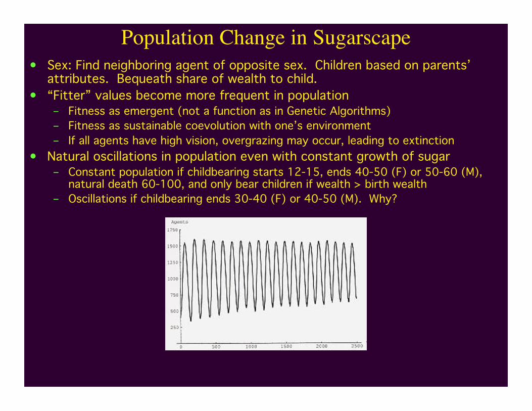
Population Change in Sugarscape• Sex: Find neighboring agent of opposite sex. Children based on parents’

attributes. Bequeath share of wealth to child.• “Fitter” values become more frequent in population

– Fitness as emergent (not a function as in Genetic Algorithms)– Fitness as sustainable coevolution with one’s environment– If all agents have high vision, overgrazing may occur, leading to extinction

• Natural oscillations in population even with constant growth of sugar– Constant population if childbearing starts 12-15, ends 40-50 (F) or 50-60 (M),

natural death 60-100, and only bear children if wealth > birth wealth– Oscillations if childbearing ends 30-40 (F) or 40-50 (M). Why?

Cultural Transmission in Sugarscape• Cultural heritage: series of 1 and 0 tags. E.g. 100010010• Transmission: Randomly select one tag and flip it to neighbor’s

value• Cultural groups by tag majority rule: Red group if 1s>0s, else Blue

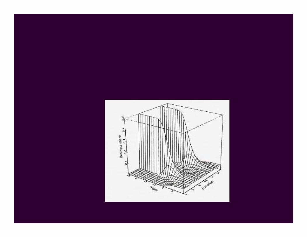
– Considerable variability within a group• Typical behavior: one group dominates over time• Friend if similar and neighbor. Friends tend to stay close

– Does similarity affect who we interact with? (Coleman, 1965) - adoptfriend’s smoking habits, and choose friends by habits

– Does similarity affect proximity or vice versa?– Are all agents equally connected? Hubs?– What is the role of far friends? Small-worlds?– Does group affect tags? Greater coherence with time?

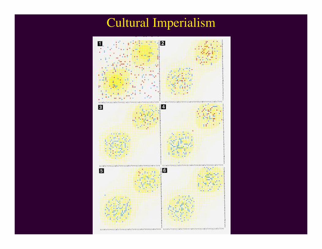
Cultural Imperialism

Friends stay close

Social Influence• Groups do not always regularly increase their uniformity over time

– Minority opinions continue to exist– Group polarization: sub-groups resist assimilation– Contrast with rich-get-richer models of cultural transmission

• Social influence on opinion– Conformity (Sherif, Asch, Crutchfield, Deutsch & Gerard)– Active community association members correlate better with their

community’s vote (.32) than nonmembers (0) (Putnam, 1966) -marginalization

– MIT housing study with random court assignments (Festinger, 1950)• 38% of residents deviated from modal attitude within housing court• 78% of residents deviated from cross-court attitude

• Four characteristics of group opinion– Consolidation: reduction of diversity of opinion over time– Clustering: people become more similar to their neighbors– Correlation: attitudes that were originally independent tend to become

associated (social and economic conservatism)– Continuing diversity: Clustering protects minority views from complete

consolidation

Sherif (1936) norms

When judge amount of movement of a point of light (autokineticeffect), estimates converge when made in group

Nowak’s Celluar Automata Model of Social Influence• Each person is a cell in a 2-D cellular automata• Each person influences and is influenced by neighbors• Immediacy = proximity of a cell• Attitude: 0 or 1• Persuasiveness = convince others to switch: 0-100• Social support = convince others to maintain: 0-100• Change opinion if opposing force > supporting force

†

NO

12

Pi

di2

i=1

NO

ÂNO

Ê

Ë

Á Á Á Á

ˆ

¯

˜ ˜ ˜ ˜

> NS

12

Si

di2

i=1

NO

ÂNS

Ê

Ë

Á Á Á Á

ˆ

¯

˜ ˜ ˜ ˜

NO=Number of opposing neighbors, Pi= Persuasivenessof neighbor i, Si= supportiveness of neighbor i,di=distance of neighbor i

•Does everybody have same number ofneighbors? Hubs?

•Does everybody only connect toneighbors? Small-worlds?

•Is assumption of no movementplausible or innocuous?

•Are attitudes well represented by asingle binary bit?

•Is there a reaction-formation tomajority opinions?

Consolidation increases with time

Polarization: Small deviations from 50% are accentuated