SNP chips Advanced Microarray Analysis Mark Reimers, Dept Biostatistics, VCU, Fall 2008.
14
SNP chips Advanced Microarray Analysis Mark Reimers, Dept Biostatistics, VCU, Fall 2008
-
date post
21-Dec-2015 -
Category
Documents
-
view
218 -
download
0
Transcript of SNP chips Advanced Microarray Analysis Mark Reimers, Dept Biostatistics, VCU, Fall 2008.

SNP chips
Advanced Microarray Analysis
Mark Reimers,
Dept Biostatistics, VCU, Fall 2008

Affy SNP chips

SNP Chip Probe Design
• 10 25-mers overlapping the SNP
• Alleles A & B• Sense and Anti-sense
– or PM and MM (old)

RMA for SNP chips
• Initial Affy software wasn’t very accurate
• Rabbee & Speed (2006) proposed RLMM, an RMA-like method using:– Quantile normalization– Two variables ( A & B signals)– Discriminant analysis
• Much better than Affy software
• Variant (BRLMM) adopted by Affy

Discriminating SNPs
• Estimate common covariance to clusters on ‘training’ set (Hapmap) data
• Separate clusters by Mahalanobis metric • Use pre-defined clusters & metric to tell apart
alleles on new data

Success Rate
• 90% (MPAM) to 98% (CRLMM) called at comparable accuracy on HapMap data– Cross-validation estimate
• BUT
• New chips don’t
have same distributions
as ‘training’ set

CRLMM - a heroic solution
• RLMM couldn’t be extended across labs
• Still problems with several hundred SNPs
• CRLMM addresses both these issues by careful normalization
• Achieves accuracy of 99.85% on hets; 99.95% on homozygotes
• Most complicated statistical calculation in BioC!

CRLMM Overview
1. Normalize intensity on each chip separately by
2. Summarize ,
, ,
by median polish: M+ =
- ; M- =
-
3. Model log ratio bias on each chip by
4. Estimate log ratio bias using E-M
– Where Zi indexes which SNP state is likely
– k = 1,2,3 for AA, AB, BB

Normalization – Step 1
• Regress (PM) intensity on sequence predictors and fragment length
hb(t) for all four bases on two chipsg(L) and 95% CI on one chip

Normalization – Step 1• Too many hb(t)’s
– Impose constraint:• hb(t) is a cubic spline with 5 df on [1,25]
• Forces neighboring values of h to be close• Allows variation in smoothness (unlike loess)
• Subtract fitted values from signal
• BUT: bias still present

Step 2 – Summarization
• Median Polish– Tukey’s exploratory method for arrays of
numbers– Iterative method
• Subtract medians of each row and each column (and accumulate) until medians converge
• Robust
• Fast

Step 3 – Ratio Normalization
• Fit bias function:– of form:
• reflects allele bases
• But what is k?
• Estimate by E-M
fL(L) for one chip
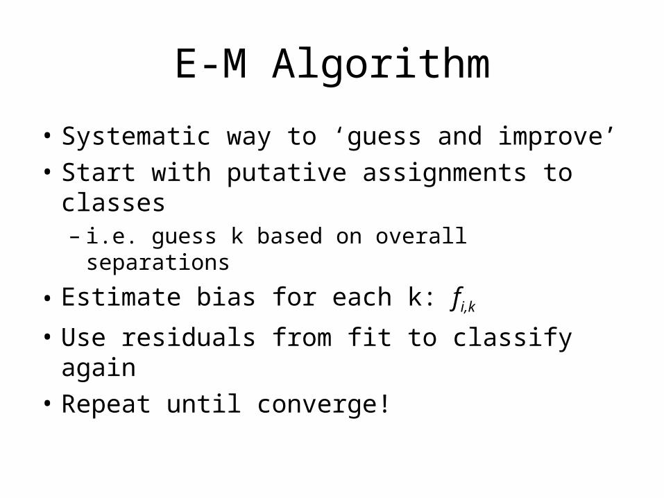
E-M Algorithm
• Systematic way to ‘guess and improve’
• Start with putative assignments to classes– i.e. guess k based on overall separations
• Estimate bias for each k: fi,k• Use residuals from fit to classify again
• Repeat until converge!

Final Step: Calling
• Aim: separation in two-dimensional log-ratio space:
• Accuracy > 99.85% on all Hapmap calls