Snow Runoff Modeling Using Meteorological,...

Intl. J. Humanities (2013) Vol. 20 (2): (79-100)

79

Snow Runoff Modeling Using Meteorological,

Geological and Remotely Sensed Data

Nastaran Saberi1, Saeid Homayouni2, Mahdi Motagh3

Received: 2012/3/5 Accepted: 2013/1/1

Abstract

Geographic information and analysis provide a wide range of data and techniques

to monitor and manage natural resources. As an important case, in arid and semi-

arid areas, water management is critical for both local governance and citizens. As

a result, the estimation of potential water brought by snowmelt runoff and rainfalls

has a significant importance for these dry areas. Hydrological modeling needs vast

knowledge about integrating all relating parameters. In this work, different data

sources including remote sensing observations and meteorological and geological

data are integrated to supply spatially detailed inputs for snowmelt runoff modeling

in a watershed located in Simin-Dasht basin in the northeast of Tehran, Iran.

Because of high temporal frequency and suitable spatial coverage, MODIS

products have been chosen to derive snow cover area. The MODIS 8-day snow

map product with an spatial resolution of 500m (MOD10A2.5) is used. In addition,

during the snowmelt period in 2006-2007, archived meteorological and geological

data are used to provide parameters and variables for empirical Snow Runoff

Modeling (SRM). Landsat ETM+ images with a higher spatial resolution of 30m

and less temporal coverage of 16 days are used in 2007 snowmelt period to

compare the model accuracy using snow cover area estimations from different

sources. Evaluation of the runoff outputs in both models, using in situ

measurements, reveals good agreements that prove SRM capability in modeling

basin’s daily and weekly runoff. Model accuracy shows better satisfactory of snow

runoff modeling results that employ Snow Cover Area (SCA) derived from

1 PhD student, RS, Department of Geography, University of Waterloo, [email protected] 2 Assistant Professor, Department of Geography, University of Ottawa, [email protected] 3 Assistant Professor, Department of Geomatics, University of Tehran, [email protected]

Snow Runoff Modeling Using Meteorological… Intl. J. Humanities (2013) Vol. 20 (2)

80

Landsat ETM+ data compared to MODIS snow product modeling. Although, using

MODIS SCA the model accuracy was less, still due to less further process and

providing better temporal coverage during snowfall and snowmelt season MODIS

is recommended. Future works in this criterion could be concentrated on SRM

forecast improvement using data assimilation techniques or coupling the empirical

model to physical models.

Keywords: Snowmelt Runoff Modeling; MODIS; Landsat ETM+; Snow Cover Area; Meteorological

Data.

1. Introduction

Forecasts related to water cycle are highly

affected by seasonal snow cover. Melted

water from a snowpack or ice layer reserve

soil humidity in mountainous catchments

and this will be continued till the end of

melting season (DeWalle and Rango,

2008). Using remote sensing observations

in monitoring snow cover area and thus

modeling snowmelt runoff is an efficient

monitoring technique that is attributed to

the high spatial and temporal variability of

snow cover (Nagler, Rott et al., 2008). In

addition, gathering in-situ measurements of

snow physical properties in high spatial and

temporal details and over big basins is not a

feasible way for providing suitable required

data for modeling (Liang, 2008).

Many models have been used to

calculate and forecast snow runoff. Models

for snow properties and runoff retrieval are

divided into empirical and physical

approaches. Physical models are more

sophisticated and can be used for different

areas without critical changes and

calibration needed. The only drawback is

their requirements; these models have many

parameters and variables, which make them

not quite applicable in some cases. One

example of physical models that has been

widely used is the energy balance model.

The second group is empirical models in

which empirical formulas and relations are

used to model the runoff amount. In

comparison with physical models, empirical

models require less parameters and

variables, so applying these models is faster

and easier. A disadvantage of empirical

models is requiring calibration for different

Saberi N. and others Intl. J. Humanities (2013) Vol. 20 (2)

81

study areas, which then results “home -

made” versions.

In this paper, an empirical snowmelt

runoff modeling, SRM1 developed by

Martinec (Martinec, Rango et al., 1998) has

been employed. Due to high temporal

frequency and suitable spatial coverage of

MODIS optical images, MODIS 8-day

snow map product with spatial resolution of

500m (MOD10A2.5), has been chosen to

map snow cover. Archived meteorological

and geological data are used to provide

SRM parameters and variables. Landsat

ETM+ images with better spatial resolution

(30m) and less temporal coverage (16 days)

are also used to compare the model

accuracy in same conditions. A review on

snow mapping via remote sensing

techniques and study area description are

brought in sections 2 and 3 respectively.

Then implied methodology as well as

results and conclusion have been discussed

in sections 4, 5, and 6, respectively.

2. Literature Review

Hitherto, the Runoff Model (SRM) by

Martinec (Martinec, Rango et al., 1998) is

the only widely empirical applied model

1 Snowmelt Runoff Model

optimized for remotely sensed snow cover

data as an input variable (Najafzadeh,

Abrishamchi et al., 2004). In this model, the

snowmelt is calculated using the SCA

derived from remotely sensed images with

respect to degree-days. Most of the other

models, such as physical models, need

estimation of various parameters and

measuring many variables to calculate the

net energy that melts the snowpack.

Due to large possibilities of exploiting widely different parts of the electromagnetic spectrum to learn more about the snowpack resource, monitoring snow surface and its hydrological properties can be performed using various satellite images. In the visible spectrum, fraction of the basin covered by snow could be mapped because of the difference in reflectance of snow and snow-free areas. The near infrared portion can also be used for snow mapping and for the detection of near surface liquid water. In the microwave portion, the snowpack emission and attenuation depend on the size and shape of crystals and the presence of liquid water (DeWalle and Rango, 2008).

Snow detection based on optical images was the first step in this application. It has been done through visual interpretation and manual digitizing on Landsat Multi Spectral


82

Scanner Images (Rango, 1980). Around ten years afterwards, snow cover digital mapping procedure has been replaced with the manual digitizing (Baumgartner and Apfl ,1994; Michael and Baumgartner, 1995). To improve the SCA accuracy, fractional snow cover algorithms are applied to estimate SCA in sub pixel resolution (Dadashi khanghah and Matkan, 2007; Dobreva and Klein, 2011).

Thermal infrared remote sensing has minor potential for snow mapping and snow hydrology. On the other hand, passive microwave radiometry have been used widely to estimate the snow properties such as Snow Water Equivalent (SWE) (Vuyovich and Jacobs, 2011). Moreover, active microwave sensors, especially Synthetic Aperture Radar (SAR) have been also used widely to estimate snow properties. In addition the microwave imagery can help to discriminate easily the snow from other surfaces (Elachi and Van Zyl, 2006; Liang, 2008).

In recent years, fusion methods have been utilized in multi-sensor approaches for monitoring SCA and Snow Surface Wetness (SSW). This has been resulted in developing data assimilation techniques to operationally forecast the runoff in short-term by satellite-based remote sensing techniques (Solberg, Koren et al., 2010).

3. Study Area The Firuzkuh area, (34 N, 51 E) is a 1576Km2 catchment to the Hablerud River in south of Alborz Mountains and North-East of Tehran, Iran. This basin altitude ranges from 980 to 4036 m. This basin is chosen for snow runoff modeling with respect to high amount of snow cover area during cold season and consequently high amount of melted water in spring. Figure 1 shows the location of this basin.

Figure 1. Study area location

4. Methodology 4.1. Datasets

Using SRM, required parameters and

variables should be supplied. These


83

requirements include satellite data, in-situ

measurements and ancillary maps.

Datasets used in this study that have been

categorized in three groups, are described

in Figure 2.

Datasets

Satellite Data Meteorological and hydrological data

Geological data and topography information

MODIS 8-day snow product

Landsat ETM+ images

Mean daily temperature – meteorology station

Daily runoff information - hydrological stations

Daily rainfall and snowfall information - rain and snow gauge

stations

DEM

Land use

Soil classification

Figure 2. Various datasets used for the snow runoff modeling

4.2. Pre-Process Pre-process contain several steps to derive

model requirements. The information

includes parameters and variables required

to model snowmelt runoff. Figure 3 shows

pre-process steps for the three datasets

mentioned in the dataset section.

Aforementioned steps are described in

subsections 3.2.1 to 3.2.3.

Figure 3. Pre-process steps to derive model input requirements

Topography

Meteorological - Geological and Land-Use Data

HRU Classification

Degree- Day Factor Curve Number Value Runoff Coefficients

Remote Sensing Data

Snow Cover Area


84

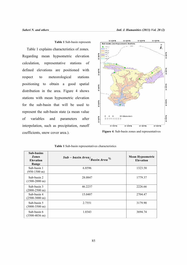
4.2.1. Topography

The altitude of the basin ranges from 980 to

4036 meters and 6 sub-basins zones or

HRU (Hydrological Response unit) are

derived as shown in Figure 4. The mean

hypsometric elevation of the zone (which is

also called mean elevation for ease of use)

determined by an area-elevation curve

using the Digital Terrain Model (DTM) of

the basin with balancing the area below and

above the mean elevation. ASTER1 DTM

data with spatial resolution of 30 meters has

been used after a Fill Sink correction pre-

process in ArcGIS software.

1The Advanced Space borne Thermal Emission and Reflection Radiometer


85

Table 1 Sub-basin representatives characteristics

Table 1 explains characteristics of zones.

Regarding mean hypsometric elevation

calculation, representative stations of

defined elevations are positioned with

respect to meteorological stations

positioning to obtain a good spatial

distribution in the area. Figure 4 shows

stations with mean hypsometric elevation

for the sub-basin that will be used to

represent the sub-basin state (a mean value

of variables and parameters after

interpolation, such as precipitation, runoff

coefficients, snow cover area.).

Figure 4. Sub-basin zones and representatives

Table 1 Sub-basin representatives characteristics

Sub-basins Zones

Elevation Range

𝑺𝒖𝒃 − 𝒃𝒂𝒔𝒊𝒏 𝑨𝒓𝒆𝒂𝑩𝒂𝒔𝒊𝒏 𝑨𝒓𝒆𝒂% Mean Hypsometric

Elevation

Sub-basin 1 (950-1500 m)

6.8596

1323.58

Sub-basin 2 (1500-2000 m)

28.0847

1779.37

Sub-basin 3 (2000-2500 m)

46.2237

2226.66

Sub-basin 4 (2500-3000 m)

15.0407

2704.47

Sub-basin 5 (3000-3500 m)

2.7551

3179.90

Sub-basin 6 (3500-4036 m)

1.0343

3694.74


86

4.2.2. Meteorological and Geological Data

Meteorological data includes daily rainfall

and runoff, mean daily temperature and

snow properties. This dataset has been

collected from synoptic and climatologic

stations as wells as in-situ measurements.

TIN1 interpolation was applied on

meteorological data to derive daily

variables for the whole basin. Best station

selection to enter interpolation process was

done using 2 and 5 kilometers buffer

analysis (nearest stations), stations in a 5

kilometer buffer were added only if they

had similar geological data (soil hydrologic

group and land-use), while compared to the

mean elevation representative station.

The geological data is then used to

classify the hydrologic soil group (A-to-D) with respect to tables given by Cronshey et

al., (1986) for the classification of different

materials in soil groups and for Curve

Number (CN) calculation considering the

land-use data. The CN is an index for

computation of basin’s Lag Time (Tlag),

potential maximum soil moisture retention

and runoff coefficients (Cronshey et al.,

1. Triangulated Irregular Network

1986). In this research, we used CN

relations with runoff coefficients; applied

empirical formulas are included at the end

of this section. However there are different

methods that are more sophisticated for

runoff coefficients derivations compared to

the method that is used here, but these

models need more variables to be

measured.

The soil CN values, for every of 50 by

50 meter pixel, are computed by

rasterizing hydrologic soil group and

different land-use classes maps. Result's

cell values contain, Soil Hydrologic group

+ Land-use class *10, which could be

transformed to curve number value using a

look-up table of curve numbers for each

land-use class and corresponding soil

hydrologic group (Cronshey et al., 1986).

Using CN raster map, average values are

computed for each sub-basin. Hydrologic

soil group and different land cover/use

classes in the region are shown in Figure 5

and Figure 6.


87

Figure 5. Soil hydrologic group Figure 6. Land-use class

CN can be used to calculate S-potential

maximum soil moisture retention (in

inches) by equation (1).

s = 1000CN

−10 (1)

Then lag time is estimated by equation

(2), which is the time difference between

the start of increasing temperatures and the

corresponding increase in runoff from the

basin (Martinec, Rango, and Roberts,

1994). Lag time is mainly determined from

the hydrographs of the past years, but lack

of this knowledge leads us to apply

empirical formula developed by Soil

Conservation Service (SCS) of United

States (Cronshey et al., 1986).

Tlag =L0.8(S +1)0.7

1900y0.5

(2)

In this formula, L is the maximum river

length of the basin (in feet) and y is the

average slope of basin (%). Tlag will be

obtained in an hourly unit and should be

rounded by the nearest integer value. In

equations (3) to (6), examples of Tlag usage

in the SRM have been brought (Martinec et

al., 1994). It shows contributions of input

on the nth day (In) and n+1th (In+1) day with

different lag times, which results in Qn+1/

Qn+2 day's runoff after being processed by


88

the SRM. In our study area Tlag was

estimated 5.6, so equation (3) used for SRM

process.

Tlag =6h , 0.50.In +0.50.In+1→ Qn+1

(3)

Tlag =12h , 0.75.In +0.25.In+1 → Qn+1

(4)

Tlag =18h , In→ Qn+1 (5)

Tlag =24h , 0.25.In +0.75.In+1→ Qn+2

(6)

Runoff coefficients (rainfall and snow)

are then computed by the equation (7),

resulted from fraction of runoff height to

precipitation height (P is precipitation

height in inches) and runoff height is

derived by the equation (8).

C = RP

(7)

R = (P − 0.2S)2

(P + 0.8S)

(8)

4.2.3. Optical Remotely Sensed Images

For this study, the MODIS’s 8-day product,

with a 500m spatial resolution, is used to

determine the SCA. This product has the

lowest percent of cloud coverage, due to

monitoring of maximum snow extent

during eight consecutive days. Landsat

ETM+ images with a higher spatial

resolution and a lower temporal resolution

are also used to compare the results of

models with different inputs of SCA.

4.2.3.1. MODIS Snow Product

The Moderate Resolution Imaging Spectro-

radiometer (MODIS) snow products are

provided in a swath and tile format and

different spatial and temporal

transformation, e.g., 8-day 500 meters

spatial resolution product (Zhang, 2004;

Riggs, Hall et al., 2007). The MOD10A2.5

product is available in global coverage and

8-day composite that has less cloud pixels

in maximum 8-day snow-extent dataset and

could lead to a more accurate snow cover

map. The pixel values that depict the

maximum of snow cover are used due to an

unstable climate condition in the

mountainous regions (Riggs and Hall,

2011).

To obtain the best estimation, the snow

product has been ignored in the condition

that cloud cover percentage in the basin is

more than 10% of the basin. The SCA is

then interpolated using the linear method to

obtain the daily snow cover in the condition


89

that the temperature is lower than snowmelt

critical degree (Tc). For higher temperature

degrees, SCA is calculated using equations

(9) and (10). Where, ∆𝑀 is volume of

melted water between t1 and t2, a is degree-

day factor and 𝑇! is a counter for degrees

higher than Tc.

ΔM (t1, t2 ) = aT +

t1

t2

∑ (9)

SCA(tx ) = SCA(tx−1)−SCA(t1)− SCA(t2 )

ΔM (t1, tA )+ΔM (tE, t2 )ΔM (tx−1, tx )

(10)

a, degree-day factor, indicates the

snowmelt depth resulting from one degree-

day and is obtained by an empirical

equation:

a =1.1 ρsρw

(11)

where, 𝜌! is the snow density and 𝜌! is

the water density. Using in-situ

measurements degree-day factor calculated

for specific dates and interpolated for snow

season during each ten days period. Tc,

snowmelt critical degree is a discriminator

of measured or forecasted precipitation type

(rain/snow). Due to lack of comprehensive

information, Tc has been determined in a

range of 0 to 3° c with respect to basin

climate and last studies done (Martinec et

al., 1994).

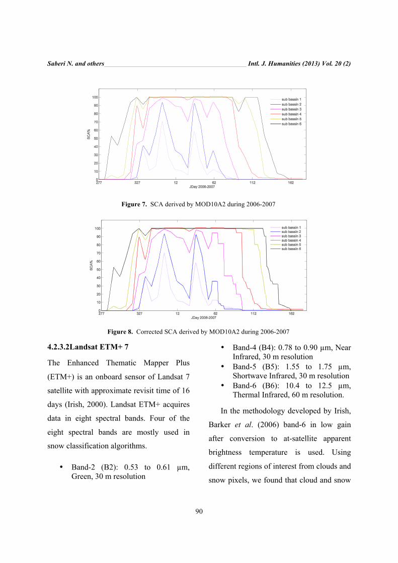
Figure 7 shows SCA percentage in the

sub basins during 2006-2007 periods. Snow

depletion curve correction, with respect to

degree-day factor and daily temperature

above the critical temperature in melting

season is applied. Depletions curves in the

six HRUs are shown in Figure 8.


90

Figure 7. SCA derived by MOD10A2 during 2006-2007

Figure 8. Corrected SCA derived by MOD10A2 during 2006-2007

4.2.3.2Landsat ETM+ 7

The Enhanced Thematic Mapper Plus

(ETM+) is an onboard sensor of Landsat 7

satellite with approximate revisit time of 16

days (Irish, 2000). Landsat ETM+ acquires

data in eight spectral bands. Four of the

eight spectral bands are mostly used in

snow classification algorithms.

• Band-2 (B2): 0.53 to 0.61 µm, Green, 30 m resolution

• Band-4 (B4): 0.78 to 0.90 µm, Near Infrared, 30 m resolution

• Band-5 (B5): 1.55 to 1.75 µm, Shortwave Infrared, 30 m resolution

• Band-6 (B6): 10.4 to 12.5 µm, Thermal Infrared, 60 m resolution.

In the methodology developed by Irish,

Barker et al. (2006) band-6 in low gain

after conversion to at-satellite apparent

brightness temperature is used. Using

different regions of interest from clouds and

snow pixels, we found that cloud and snow


91

temperature are close together and even

overlap in some areas. Consequently, the 6th

band information was not used in the

classification algorithm. Level 1

Geometrically corrected product has been

used to obtain SCA from each image. It

should be noted that from 2003, ETM+

Scan Line Corrector (SLC) has been out of

order and as a result all captured images

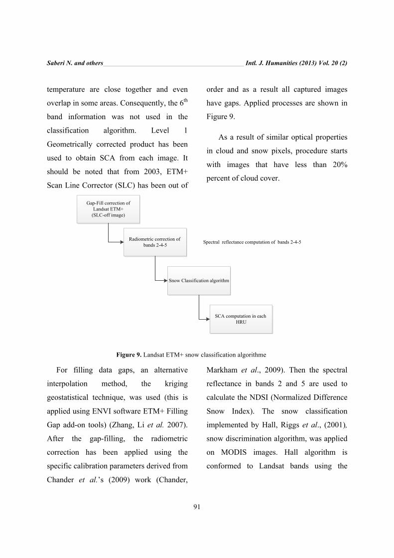
have gaps. Applied processes are shown in

Figure 9.

As a result of similar optical properties

in cloud and snow pixels, procedure starts

with images that have less than 20%

percent of cloud cover.

Figure 9. Landsat ETM+ snow classification algorithme

For filling data gaps, an alternative

interpolation method, the kriging

geostatistical technique, was used (this is

applied using ENVI software ETM+ Filling

Gap add-on tools) (Zhang, Li et al. 2007).

After the gap-filling, the radiometric

correction has been applied using the

specific calibration parameters derived from

Chander et al.’s (2009) work (Chander,

Markham et al., 2009). Then the spectral

reflectance in bands 2 and 5 are used to

calculate the NDSI (Normalized Difference

Snow Index). The snow classification

implemented by Hall, Riggs et al., (2001),

snow discrimination algorithm, was applied

on MODIS images. Hall algorithm is

conformed to Landsat bands using the

Gap-Fill correction of Landsat ETM+

(SLC-off image)

Radiometric correction of bands 2-4-5

SCA computation in each HRU

Snow Classification algorithm

Spectral reflectance computation of bands 2-4-5


92

equation 12. The output class labels is 0 for

no snow and 1 for snow class.

Snow=NDSI>0.4&b4>011&b2>0.1 (12)

Moreover, snow detection based on the

Automatic Cloud Cover Assessment

Algorithm (ACCA) algorithm is applied

using:

Snow=NDSI>0.7 . (13)

The classification’s overall accuracy in

the scene, with 60% percent of cloud cover,

was 95.6% and 87.8% with first and second

method as described above (equations (3)

and (4)). To estimate the accuracy, snow

pixels are collected with respect to

interpolated temperature and specific visual

pattern of snow. Due to the better results of

conformed Hall snow classification; this

method is applied on all images obtained

during 2006-2007. Figure 10 shows results

of both algorithms for Landsat image of

2006/10/23.

a B

Figure 10. a) Landsat Image (RGB:345), b) SCA derived from Eq 3, c) SCA derived from Eq 4

Figure 11 shows the SCA fraction in the

sub-basins during 2006-2007 using ETM+

images; interpolated linearly for days that

no images were available. The daily SCA

fraction during the snowmelt season in

2007 for 6 HRU is derived and Snow

depletion curve correction is applied with

respect to the degree-day factor and daily

temperature above the critical temperature

in the melting season. Corrected depletions

curves in 6 HRU using ETM+ images are shown in the Figure 12. It should be noted

that differences between the SCA retrieved

from MODIS snow product and Landsat

images are due to calculating of maximum

snow extent in MODIS snow product,

which leads to an accuracy fall due to

obtaining SCA in fewer time intervals.


93

Figure 11. The SCA derived from Landsat ETM+ during 2006-2007

Figure 12. The corrected SCA Derived from Landsat ETM+ during 2006-2007

4.3. Snow Runoff Model (SRM)

The Snowmelt Runoff Model (SRM)

developed by Martinec, Rango et al.,

(1998) is used in this study for runoff

modeling in our study basin. This model

has been applied in more than 100 basins in

29 different countries around the world with

various areas from 0.8 km2 to 917,444 km2

(Martinec, Rango et al. 1998). SRM is a

degree-day based deterministic hydrologic

model that simulates daily snowmelt and

rainfall runoff in mountainous basins.

Required input variables for SRM includes

daily temperature, precipitation and snow

covered area. The daily runoff is computed

using (Martinec, Rango et al. 1998):


94

Qn = KnQn−1 +

(1−Kn )1000086400

[CSi,nai,n (Ti,n +ΔTi,n )Si,n +CRi,nPi,n ]Aii

∑

(14)

In this equation, n is the day number; i is HRU index; k is the recession coefficient; CS is the snowmelt runoff loss factor; CR is the rainfall loss factor; T+∆T is the air temperature above the threshold of melt including measured temperature in station plus temperature correction for mean elevation station minus critical temperature; P is the precipitation amount falling as rain or snow and A is the area.

The recession coefficient equals to the ratio of runoff on consecutive days when there is no added snowmelt and rain runoff. It can be computed from an archived runoff data as a function of Q, so that nonlinearity of the storage can be explained (Nagler, Rott et al. 2008). To derive k, archived basin’s runoff in nth day is plotted against n+1th day; it has been shown in Figure 13. Then slope and y intercept of the fitted line, calculated by weighted least squares method, are used in the equation (15) (Martinec et al., 1994).

Kn+1 = aQn−b (15)

Figure 13. Stream Discharge 𝐐𝐧 against 𝐐𝐧!𝟏 and Fitted Line

where, a is slope, b is y intercept and Q!

is nth day runoff.

Interpolation methodology used for T and P distributed measurement and degree-day factor and runoff coefficients calculation were described in the section 3.2.1. Fraction of snow cover measurement explained in 3.2.2. Mean values of these variables and parameters for each HRU is then employed in the SRM (Martinec, Rango et al., 1998; Nagler, Rott et al., 2008). 5. Results and Discussion


95

SRM is performed for the water year 2006-2007. Model accuracy is explored by R2, a measure of model efficiency and Dv according to equations (16) and (17), respectively (Martinec, Rango et al., 1998).

DV =VR − "VRVR

*100 (16)

R2 =1−(Qi − "Qi )

2

i=1

n

∑

(Qi −Q)2

i=1

n

∑

(17)

Figure 14 includes the measured and modeled runoff and accuracy parameters using corrected SCA driven from MODIS 8-Day product. Figure 15 includes measured and modeled runoff and accuracy parameters using corrected SCA driven from Landsat images.

Figure 14. Daily SRM using MODIS snow Product (JDay starting from 2006-2007 water year)

Figure 15. Daily SRM using landsat ETM+ images (JDay starting from 2006-2007 water year)


96

Differences between measured and modeled runoff are observed mainly before the snowmelt season, when the runoff is as a result of the rainfall and not the snowmelt water. Moreover, after a heavy rainfall modeling the response of basin needs more investigations.

Results show that this approach has the potential to be implemented in a prototype project for monitoring SCA and even forecasting snowmelt runoff in a web based interface system for the end users in this field of interest (it should be noted that forecasting needs data assimilation using climatologic data). For instance, snow runoff modeling can be useful in water management for both managers and users while irrigation schedule would be defined through the knowledge of estimated runoff at the end of season. Weekly and bi-weekly forecasts can be computed using the average temperature degree, precipitations and SCA during last ten years to adapt and calibrate SRM for a specific case study. SCA driven from MODIS product due to its application usage and also ease of access and process can be useful in this application.

6. Conclusion

In this study, SRM over a mountainous

watershed in south of Ablorz Mountain and

Hableh-Roud river basin has been

implemented. Various data including

meteorological data, geological maps and

remotely sensed image data are processed

to provide the inputs of SRM. Two different

optical images were used in the snowmelt

modeling for a SCA calculation to reach

better accuracy in daily runoff modeling.

Albeit, Landsat revisit time is 16 days and

MODIS revisit time is 12 hours, SCA

derived from Landsat images shows better

agreement in measured runoff especially in

melt season due to a better pixel resolution

(30 meters versus 500 meters). However,

SRM should be applied for several years to

define whether using Landsat for snowmelt

modeling will result in a more accurate

modeling compared to MODIS snow maps.

Due to free access to high level processed

MODIS snow maps and also high temporal

frequency compared to Landsat, using

MODIS products in runoff modeling is

more beneficiary in hydrological

applications and is preferable compared to

Landsat images.

One of the SRM's weaknesses is

assuming a snowpack layer as a

homogenous medium with uniform

properties. Using field experiments to


97

obtain more information during snowmelt

season and modeling snowpack properties

in addition to SCA could be helpful in daily

SRM improvement. This information is also

an important requirement in snowmelt

forecast applications, when dynamic

changes in snow grain size and density in

different days of year (seasonal snowpack

evolution) and from year to year affect

estimations accuracy.

In addition, different satellite images and

synoptic meteorological data using fusion

and assimilation methods, respectively

could be utilized to improve the model. For

instance, fusion of visible images with SAR

images and LST1 products in decision level

could be an effective approach in this

criterion. SCA could also be improved

using fractional snow cover estimation by

unmixing methods. As SWE estimation is

possible using microwave spectrum due to

microwave penetration ability in snowpack

layers, some more investigations should be

also done for re-sampling methods on

passive products for better integration with

higher spatial resolution dataset to be

utilized in such runoff models.

1 Land Surface Temperature

Acknowledgement

This work has been funded by Semnan

Water Management Organization. We

express our gratitude to Mr. Abyati,

Khamoushi and Taheri for their helpful

suggestions. We also thank NASA and

UGSG for providing free Landsat and

MODIS data. References

[1] Baumgartner, M. F. and G. Apfl (1994),

Monitoring snow cover variations in the

Alps using the Alpine Snow Cover

Analysis System (ASCAS). Mountain

environments in changing climates.

Routledge, New York, New York, USA,

108-120.

[2] Chander, Gyanesh, Brian L. Markham, and

Dennis L. Helder. (2009), "Summary of

current radiometric calibration coefficients

for Landsat MSS, TM, ETM+, and EO-1

ALI sensors." Remote Sensing of

Environment 113(5): 893-903.

[3] Cronshey, R., H.Mccuen, R., Miller, N.,

Rawls, W., Robims, S., & Woodward, D.,

(1986), Urban Hydrology for Small

Watersheds.

[4] Dadashi khanghah, S. and A. A. Matkan

(2007), Snow cover detection using Image

processing algorithms in Karaj and latian

Basins (In Persian). Faculty of Earth


98

Sciences. Tehran, Shahid Beheshti

University. Msc.

[5] DeWalle, D. and A. Rango, (2008),

Principles of snow hydrology, Cambridge

University Press.

[6] Dobreva, I. D. and A. G. Klein, (2011),

"Fractional snow cover mapping through

artificial neural network analysis of

MODIS surface reflectance." Remote

Sensing of Environment.

[7] Elachi, C. and J. Van Zyl, (2006),

Introduction to the physics and techniques

of remote sensing, John Wiley and Sons.

[8] Hall, D. K., Riggs, G. A., Salomonson, V.

V., Barton, J. S., Casey, K., Chien, J. Y.

L., ... & Tait, A. B. (2001), "Algorithm

theoretical basis document (ATBD) for the

MODIS snow and sea ice-mapping

algorithms." Sep.

[9] Irish, R., (2000), "Landsat 7 science data

users handbook." National Aeronautics

and Space Administration.

[10] Irish, R. R., Barker, J. L., Goward, S. N., &

Arvidson, T. (2006), "Characterization of

the Landsat-7 ETM Automated Cloud-

Cover Assessment (ACCA) Algorithm."

Photogrammetric Engineering & Remote

Sensing 72(10): 1179-1188.

[11] Liang, S. (2008). Advances in Land

Remote Sensing: System, Modelling,

Inversion and Application, Springer.

[12] Martinec, J., Rango, A., & Roberts, R.,

(1994), Snowmelt runoff model (SRM)

user’s manual. Retrieved from

http://www.mastergardeners.nmsu.edu/pub

s/research/water/SRMSpecRep100.pdf

[13] Martinec, J., Rango, A., Roberts, R., &

Baumgartner, M. F. (1998), Snowmelt

runoff model (SRM) user's manual,

Geograph. Inst. d. Univ.

[14] Mountain environments in changing

climates. Routledge, New York, New

York, USA: 108–120.

[15] Michael, F. and A. R. Baumgartner,

(1995), "A microcomputer-based alpine

snow-cover analysis system (ASCAS)."

Photogrammetric engineering and remote

sensing 61(12): 1475-1486.

[16] Nagler, T., Rott, H., Malcher, P., & Müller,

F. (2008), "Assimilation of meteorological

and remote sensing data for snowmelt

runoff forecasting." Remote Sensing of

Environment 112(4): 1408-1420.

[17] Najafzadeh, R., Abrishamchi, A., Tajrishi,

M., (2004), Runoff simulation with

snowmelt runoff modeling (In Persian)."

[18] Rango, A., (1980), Operational

Applications of Satellite Snow Cover

Observations." Jawra Journal of the

American Water Resources Association

16(6): 1066-1073.

[19] Riggs, G. and Hall, D., (2011), "MODIS

Snow and Ice Products, and Their


99

Assessment and Applications." Land

Remote Sensing and Global Environmental

Change: 681-707.

[20] Riggs, G. A., Hall, D. K., & Salomonson,

V. V. (2007), "MODIS Snow Products

User Guide to Collection 5." Online article,

retrieved on January 2.

[21] Solberg, R., Koren, H., Amlien, J., Malnes,

E., Schuler, D. V., & Orthe, N. K. (2010),

"The development of new algorithms for

remote sensing of snow conditions based

on data from the catchment of Øvre

Heimdalsvatn and the vicinity."

Hydrobiologia 642(1): 35-46.

[22] Vuyovich, C. and J. M. Jacobs (2011),

"Snowpack and runoff generation using

AMSR-E passive microwave observations

in the Upper Helmand Watershed,

Afghanistan." Remote Sensing of

Environment.

[23] Zhang, C., Li, W., & Travis, D. (2007).

"Gaps-fill of SLC-off Landsat ETM+

satellite image using a geostatistical

approach." International Journal of

Remote Sensing 28(22): 5103-5122.

[24] Zhang, Y., (2004). "Understanding image

fusion." Photogrammetric engineering and

remote sensing 70(6): 657-661.


100

هھھھایی هھھھوااشناسی٬، ژژئولوژژیی وو سنجش اازز ددوورریی مدلساززیی رروواانابب حاصل اازز ذذووبب برفف با ااستفاددهه اازز ددااددهه

٣۳قمعت مهھدیی ٢۲،٬هھھھمايیونی سعيید ١۱،٬صابریی نسترنن

٬، کاناددااووااترلودداانشجویی ددکتریی٬، گرووهه جغراافيیا٬، دداانشگاهه ١۱ ااستادديیارر٬،گرووهه جغراافيیا٬، دداانشگاهه ااتاوواا٬، کانادداا ٢۲

دداانشگاهه تهھرااننگرووهه مهھندسی نقشهھ بردداارریی وو ژژئوماتيیک٬، پردديیس دداانشکدهه هھھھایی فنی٬، ااستادديیارر٬، ٣۳

15/12/90تارريیخ ددرريیافت: 12/10/91 پذيیرشش: تارريیخ

آآوورریی وو تحليیل ااططالعاتت جغراافيیايیی اامکانن پايیش وو مديیريیت گسترهه منابع ططبيیعی رراا بهھ صوررتت کارراايیی جمع

اازز ااهھھھميیت بااليیی ددرر مناططق خشک وو نيیمهھ خشک کهھ مديیريیت منابع آآبب نمونهھآآوورردد. بهھ عنواانن فرااهھھھم می

هھھھا وو سرآآغازز يي ررووددخانهھ جريیانن پايیهھیی کنندههبهھ عنواانن تأميین برفي ذذخايیریی شناخت وو مطالعهھ برخورردداارر ااست٬،

مصرفف مديیريیترريیزیی وو برنامهھ ددرر مهھمی مرتفع٬، نقش وو گيیربرفف هھھھاييحوضهھ ددرر شيیريین آآبب منابع ااصلي

یی محاسبهھ وو برفف پوشش يي نقشهھ يي تهھيیهھ ددوورر اازز سنجش آآوورريي فن اازز ااستفاددهه . باکند ا میاايیف آآبب منابع

ااست. با شدهه ممکن ززميیني هھھھاييررووشش بهھ نسبت کمتریی هھھھزيینهھ صرفف با وو بزررگگ مقيیاسس ددرر برفف پارراامترهھھھايي

SRM برفف ذذووبب رروواانابب هھھھایی هھھھيیدرروولوژژيیکی اازز جملهھ مدلل توجهھ بهھ پارراامترهھھھایی گسترددهه مورردد نيیازز ددرر مدلل

(Snowmelt Runoff Model) ددرر اايین .هھھھا نيیاززمند دداانش بااليیی ااستساززیی اايین ددااددههآآوورریی وو هھھھمگنجمع

هھھھايي هھھھا٬، وويیژگي اايیستگاهه هھھھيیدرروومتريي هھھھوااشناسي٬، اايین ااططالعاتت شامل: ااططالعاتت اازز تلفيیق ااستفاددهه با تحقيیق

رروواانابب حاصل اازز ذذووبب برفف اايي٬، مقداارر ماهھھھوااررهههھھھایی مشاهھھھدااتی آآوورريي شدهه اازز ددااددههحوضهھ وو ااططالعاتت جمع

ددشت ووااقع ددرر شودد. تغيیيیرااتت سطح پوشش برفف حوضهھ آآبريیز سيیميینرراا بهھ صوررتت ررووززاانهھ محاسبهھ مي

با قدررتت MODISفيیرووززکوهه تهھراانن با ااستفاددهه اازز محصولل سطح پوشش برفف ررووززاانهھ با ااستفاددهه اازز سنجندهه

-1386) ددرر سالل آآبی MOD10A2.5متر ( 500تفکيیک مکانی شد. بهھ منظورر مقايیسهھ ااستخرااجج 1385

متر وو 30با ددقت مکانی Landsat-7ماهھھھوااررهه +ETMسنجی با ااستفاددهه اازز تصاوويیر سنجندهه ددقت برفف

مورردد ییبا تأميین پارراامترهھھھا وو متغيیرهھھھاررووزز نيیز تغيیيیرااتت سطح برفف محاسبهھ شد. 16ددووررهه باززگشت ززمانی

هھھھا٬، وويیژگي سي وو هھھھيیدرروومتريي اايیستگاههبا ااستفاددهه اازز ااططالعاتت هھھھوااشنا (SRM) رروواانابب ذذووبب برففنيیازز مدلل

یی٬، اا٬، پارراامتر سطح پوشش برفف وو پارراامتر ررططوبت برفف ااستخرااجج شدهه اازز تصاوويیر ماهھھھوااررههحوضهھهھھھايي

ساززیی مقداارر رروواانابب ررووززاانهھ مدلساززیی شد. ددقت مدلل با ااستفاددهه اازز محاسبهھ ااختالفف حجم رروواانابب ساالنهھ شبيیهھ

ساززیی وو ووااقعی محاسبهھ شد. ااررززيیابی نتايیج مدلساززیی هھ شبيیهھبستگی ددبی ررووززاانوو ووااقعی٬، وو برآآوورردد مجذوورر هھھھم

حاکی اازز تطابق باالیی رروواانابب مدلساززیی وو ووااقعی با ااستفاددهه اازز هھھھر ددوو نوعع تصويیر وو ددقت باالتر مدلساززیی با

پايیيین تر MODISااست. هھھھرچند ددقت با ااستفاددهه اازز محصولل پوشش برفف Landsatااستفاددهه اازز تصاوويیر

تر پرددااززشش با ااستفاددهه اازز اايین تر وو حجم پايیيین ربردداارریی با ددووررهه باززگشت کوتاههبودد٬، وولی بهھ ددليیل تصويی

بيینی رروواانابب با ااستفاددهه اازز تلفيیق دديیگر شودد. توسعهھ مدلل ددرر پيیش ااستفاددهه اازز اايین محصولل توصيیهھ می تصاوويیر٬،

توااند ززميینهھ تحقيیقاتت آآيیندهه باشد. هھھھایی فيیزيیکی می هھھھا وو نيیز مدلل گيیریی ااندااززهه

Snow Runoff Modeling Using Meteorological,...

Documents

Transcript of Snow Runoff Modeling Using Meteorological,...