Snake classification from images - PeerJ · Snake classification from images ... King Cobra, Common...

Snake classification from images

Alex James Corresp. 1

1 Nazarbayev University, Astana, Kazakhstan

Corresponding Author: Alex James

Email address: [email protected]

Incorrect snake identification from the observable visual traits is a major reason of death

resulting from snake bites. So far no automatic classification method has been proposed to

distinguish snakes by deciphering the taxonomy features of snake for the two major

species of snakes i.e. Elapidae and Viperidae. We present a parallel processed inter-

feature product similarity fusion based automatic classification of Spectacled Cobra,

Russel's Viper, King Cobra, Common Krait, Saw Scaled Viper, Hump nosed Pit Viper. We

identify 31 different taxonomically relevant features from snake images for automated

snake classification studies. The scalability and real-time implementation of the classifier is

analyzed through GPU enabled parallel computing environment. The developed systems

finds application in wild life studies, analysis of snake bites and in management of snake

population.

PeerJ Preprints | https://doi.org/10.7287/peerj.preprints.2867v1 | CC BY 4.0 Open Access | rec: 11 Mar 2017, publ: 11 Mar 2017

Snake Classification from Images1

Alex James12

1Nazarbayev University3

Corresponding author:4

Alex James15

Email address: [email protected]

ABSTRACT7

Incorrect snake identification from the observable visual traits is a major reason of death resulting from

snake bites. So far no automatic classification method has been proposed to distinguish snakes by

deciphering the taxonomy features of snake for the two major species of snakes i.e. Elapidae and

Viperidae. We present a parallel processed inter-feature product similarity fusion based automatic

classification of Spectacled Cobra, Russel’s Viper, King Cobra, Common Krait, Saw Scaled Viper, Hump

nosed Pit Viper. We identify 31 different taxonomically relevant features from snake images for automated

snake classification studies. The scalability and real-time implementation of the classifier is analyzed

through GPU enabled parallel computing environment. The developed systems finds application in wild

life studies, analysis of snake bites and in management of snake population.

8

9

10

11

12

13

14

15

16

INTRODUCTION17

The morbidity and mortality due to snakebite is high in many parts of the world even with the availability18

of anti-venoms. As a first-line treatment polyvalent anti-venom is injected to the snake bite victim (Warrell,19

1999). The observational evidences of the patients are taken into account in identifying snakes, however,20

most doctors are not trained to identify the taxonomy of the snake, so accuracy of detection in practice21

is very low. There is an issue of serious misreporting, the extend of which is not studied. The injected22

polyvalent anti-venom contains antibodies raised against two or more species of snake that can neutralize23

the venom injected by a single snake bite (Calvete et al., 2007; Halim et al., 2011). The part of anit-venom24

that remain non-neutralized creates a further risk to the human health, making the correct identification of25

snakes an important problem (Halim et al., 2012).26

In this paper, we propose an inter-feature product similarity fusion classifier that incorporates the27

fusion of histogram features representative of the taxonomy of the snake. As an example, we discuss here28

our results when the task was set to distinguish two major type of snake species (Elapidae and Viperidae)29

in real-time imaging conditions. The images used in our study are that of poisonous snakes collected over30

a period of 2 years from a recognized Serpentarium and are common specimens seen in the human habitat31

region.32

In general, the automated classification of snakes from images is an open research problem. We33

present features that can be used for distinguishing two different types of snake species which is found34

commonly in India, where the data for this study was collected. The database for this study, the fusion35

classifier and the feature analysis methods are the main contributions reported in this work. In addition36

to the suitability of the method in real time imaging conditions, the proposed algorithm can be used on37

offline images of snakes for example in the application of detecting the snakes identified using the help of38

bite victim to recommend medical treatment to snake bite victims.39

Background40

The recognition of snake classes from images requires the development of a gallery of images of snakes41

belonging to given classes. The snake has several sets of taxonomy features that enable the identification42

of snake classes. Obtaining an extensive collection of snake image features for the gallery is a challenge43

making the snake classification attempted in this paper a small sample classification problem. It is44

well known that nearest neighbor classifiers are robust, simple and powerful technique under such45

conditions, and forms the basis for the classifier proposed in this paper. In this section, we provide the46


Figure 1. The illustration of feature distance space in a Nearest neighbour classifier.

necessary background on nearest neighbor classifier and in the preparation of snake database for setting47

the foundation for the further sections.48

Nearest Neighbor Classfiers49

In this paper, we use a subset of the well-known nearest-neighbor classifier. The nearest neighbor classifier50

(Cover and Hart, 1967) (kNN) identifies the class of unknown data sample from its nearest neighbor51

whose class is already known. Figure 1 shows the feature distance space of test sample to the known52

gallery samples. The set of samples that have its classes prior known is used to create the gallery set. The53

unknown sample belongs the test set and the distance from this sample to the gallery samples determined54

by a distance metric. The class of the sample in the gallery that has the closest distance to the test sample55

is assigned the class of the test sample. There are several ways of calculating the distances between the56

samples and also many different ways to include or exclude the distances to determine the class. When the57

closest distance is used for determining the class of test sample, i.e. when k = 1 as shown in Fig. 1, such58

a classifier is known as minimum distance nearest neighbor classifier. When k > 1, there are different59

ways of determining the class of the unknown test sample, such as voting for the largest number of class60

samples, or weighting and voting the sample distances, or having a learning scheme to determine the61

optimal value of k.62

The popular variants of the nearest neighbour classifier include weighted kNN(Bailey and Jain, 1978),63

Condensed Nearest Neighbor(Gowda and Krishna, 1979), Reduced Nearest Neighbor(Gates, 1972),64

Model based k nearest neighbor(Guo et al., 2003), Rank nearest neighbor(Bagui et al., 2003), Modified65

k nearest neighbor(Parvin et al., 2008), Generalized Nearest Neighbor(Zeng et al., 2009), Clustered66

k nearest neighbor(Yong et al., 2009), Ball Tree k nearest neighbor(Liu et al., 2006), k-d tree nearest67

neighbor(Sproull, 1991), Nearest feature Line Neighbor(Li et al., 2000), Local Nearest Neighbor(Zheng68

et al., 2004), Tunable Nearest Neighbor(Zhou et al., 2004), Center based Nearest Neighbor(Gao and Wang,69

2007), Principal Axis Tree Nearest Neighbor(McNames, 2001), and Orthogonal Search Tree Nearest70

Neighbor(Liaw et al., 2010).71

The nearest neighbor classifiers are non-parametric and are suitable for small sample problems. Even72

when the number of sample per class is uneven or when they become as low as one(Raudys and Jain,73

1990), the classifier provides a match based on the nearest distance. Further, limiting the value of k to74

lower values removes the impact of data outliers, and improves the robustness of classification. A lower75

value of k necessitates a distance metric that can remove the effect of outliers in features.76

The features of snake images that we collect require a prior knowledge of the class and taxonomic77

significance to be selected as gallery samples. They are more generally referred to as gallery templates to78

recognize the overall classification as a template matching process. There are different possibilities and79

ways of creating gallery templates, such as by manual segmentation of the taxonomically relevant features80

or by automatic feature extraction methods. Its practically not possible to develop a fully automatic81

method of segmentation for creating the gallery of snake features as they have a large variability such as82

scaling, illumination changes, scars on the skin, aging, color changes, and pose changes. Therefore the83

gallery templates always require a manual validation before it can be incorporated into the snake database84

to be meaningfully used in the nearest neighbor classifier.85

2/15


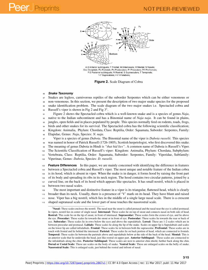
Figure 2. Scale Diagram of Cobra

Snake Taxonomy86

Snakes are legless, carnivorous reptiles of the suborder Serpentes which can be either venomous or87

non-venomous. In this section, we present the description of two major snake species for the proposed88

snake identification problem. The scale diagram of the two major snakes i.e. Spectacled cobra and89

Russell’s viper is shown in Fig 2 and Fig 31.90

Figure 2 shows the Spectacled cobra which is a well-known snake and is a species of genus Naja,91

native to the Indian subcontinent and has a Binomial name of Naja naja. It can be found in plains,92

jungles, open fields and in places populated by people. This species normally feed on rodents, toads, frogs,93

birds and other snakes for its survival. The Spectacled cobra has the following scientific classification;94

Kingdom: Animalia, Phylum: Chordata, Class: Reptilia, Order: Squamata, Suborder: Serpentes, Family:95

Elapidae, Genus: Naja, Species: N. naja.96

Viper is a species of genus Daboia. The Binomial name of the viper is Daboia russelii. This species97

was named in honor of Patrick Russell (1726-1805), Scottish herpetologist, who first discovered this snake.98

The meaning of genus Daboia in Hindi is ”that hid lies”. A common name of Daboia is Russell’s Viper.99

The Scientific Classification of Russell’s viper: Kingdom: Animalia, Phylum: Chordata, Subphylum:100

Vertebrata, Class: Reptilia, Order: Squamata, Suborder: Serpentes, Family: Viperidae, Subfamily:101

Viperinae, Genus: Daboia, Species: D. russelii.102

Feature Differences In this paper, we are mainly concerned with identifying the difference in features103

between a Spectacled cobra and Russell’s viper. The most unique and notable feature of the Indian cobra104

is its hood, which is absent in viper. When the snake is in danger, it forms hood by raising the front part105

of its body and spreading its ribs in its neck region. The hood contains two circular patterns, joined by a106

curved line, on the back of its hood which appears like spectacles. It has small nostril, which is placed in107

between two nasal scales.108

The most important and distinctive feature in a viper is its triangular, flattened head, which is clearly109

broader than its neck. Usually, there is a presence of ‘V’ mark on its head. They have blunt and raised110

nose. Viper has a big nostril, which lies in the middle of a single large nasal scale. There is a crescent111

shaped supranasal scale and the lower part of nose touches the nasorostral scale.112

1Nasal: These scales encloses the nostril. The nasal near the snout is called prenasal and the nasal near the eye is called postnasal.

In vipers, nostril lies in center of single nasal. Internasal: These scales lie on top of snout and connects nasal on both side of head.

Rostral: This scale lie on the tip of snout, in front of internasal. Supraocular: These scales form the crown of eye, and lie above

the eye. Preocular: These scales lie towards the snout or in front of eye. Postocular: These scales lie towards the rear or back of

eye. Subocular: These scales lie in rows below the eyes and above the supralabials. Loreal: These are 1-2 scales which are in

between preocular and postnasal. Labials: These scales lie along the lip of the snake. Scales on upper lip is Supralabials and scales

on the lower lip are called infralabials. Frontal: These scales lie in between both the supraocular. Prefrontal: These scales are in

touch with frontal and lie behind the internasal. Parietal: These scales lie on back portion of head, which are connected to frontals.

Temporal: These scales lie between the parietals above and supralabials below at the side of the back of the head. Mental: This is

an anterior scale that lie underside the head, just like rostral on upper part. Anterior Sublingual: These scales are connected to

the infralabials along the chin. Posterior Sublingual: These scales are next to anterior chin shield, further back along the chin.

Dorsal or Costal Scale: These are scales on the body of snake. Ventral Scale: These are enlarged scales on the belly of snake.

Nasorostral Scale: This is enlarged scale, just behind the rostral and infront of nasal.

3/15


Figure 3. Scale Diagram of Viper. Note: In any view, only one example Prefrontals and Frontals scale is

marked.

Scalation Differences The head scales of cobra shown in Fig. 2 is large compared to viper shown in113

Fig. 3. As can be seen from Fig. 2 there are rostral, 2 internasal, 2 prefrontal, 1 frontal, 2 parietals in the114

head part. There are generally 1-7 supralabial scales, which are placed along the upper lip of snake. There115

is 1 preocular and 3 postocular scale, which lies on front and back of the eye. The body scales i.e. the116

dorsal scale of the cobra is smooth.117

The head scales of viper are small as compared to cobra. They contain small frontals and some118

parietals. The supraocular scale, which acts as the crown of the eye is narrow in comparison to cobra.119

The eyes are large in size with vertical pupil. There are 10-12 supralabials, out of which 4th and 5th are120

notably larger than the remaining. They also have preoculars, postocular, 3-4 rows of subocular scales121

below their eye and loreal scale between eye and nose. Loreal scales are absent in cobra. There are122

generally 6-9 scales between both the suproculars. There are two pairs of chin shields, out of which front123

one is larger.124

The dorsal scales are strongly keeled. The dorsal scale has consecutive dark spots, which contain light125

brown spot that is intensified by thick dark brown line, which is again surrounded by light yellow or white126

line. The head has a pair of dark patches, which is situated on both the temples. Dark streaks are notable,127

behind or below the eye.128

(a) Top (b) Side (c) Bottom (d) Top (e) Side (f) Bottom (g) Body

Figure 4. Images of cobra((a)-(d)) and viper((e)-(h)). The labels indicate the feature group to which the

image belongs. Note: The images shown in this figure are resized to a common scale for display purposes.

MATERIALS AND METHOD129

Snake Database130

The snake images for the experiment were collected with the help of Pujappura Panchakarma Serpentarium,131

Trivandrum, India, through the close and long-term interaction with the subjects under study. These132

photographs don’t require ethical clearance as we took photographs from a recognized Serpentarium133

and are common specimens seen in the human habitat region. The total number of images used for this134

4/15


experiment are obtained from 5-6 snakes of each species on different occasions and time under wild135

conditions. Sample images from the database are shown in Fig. 4. Obtaining photographs under realistic136

conditions are challenging due to the dangers involved with snake bites. The problem addressed in137

pattern recognition context is a highly challenging task of small sample classification under unconstraint138

recognition environments.139

We started with a database of 88 images of cobra and 48 images of viper for the initial feature140

taxonomy analysis. Then for image based recognition the database with a total of 444 images; of141

which Spectacled Cobra (SC), Russel’s Viper(RV), King Cobra(KC), Common Krait(CK), Saw Scaled142

Viper(SSV), Hump-nosed Pit Viper (HNPV) has 207, 76, 58, 24, 36 and 43 images were used.143

Snake feature database144

Table 1. Classification of the taxonomy features based on the observer view

Feature Table

Top F1 Rostral; F2 Internasal; F3 Prefrontal, F4 Supraocular, F5 Frontal, F6 Pari-

etal, F7 V mark on head, F8 Triangular head, F9 Dark patches on both sides

of head, F10 No. of scales between supraocular

Side F11 Small nostril, F12 Round pupil, F13 Big nostril, F14 Elliptical pupil, F15

Loreal, F16 Nasorostral, F17 Supranasal, F18 Triangular brown streaks behind

or below eyes, F19 Subocular, F20 Nasal, F21 Preocular, F22 Postocular, F23

No. of Supralabial scale

Bottom F24 Mental, F25 Asterior Sublingual, F26 Posterior Sublingual

Body F27 Round Dorsal scale, F28 Hood, F29 Spectacled mark on hood, F30 Keeled

Dorsal scale, F31 Spots on Dorsal scale

Table 1 shows the proposed grouping of taxonomy features based on the observer views of the snakes145

shown in Fig. 2 and Fig. 3. In total 31 taxonomy based features are identified for creation of the feature146

database from the 136 snake images collected. There is a total of 88 images of cobra and 48 images of a147

viper. For creating the feature database, each image is translated to samples with 31 features, totalling 136148

samples for the database.149

Snake image database150

The taxonomical features can be used to construct an image only feature database from individual snake151

images. We use the taxonomical feature as outlined in Table 1, with the help of snake taxonomy to create152

image feature database. In the region of images with the specific features are cropped manually, so that153

each snake image sample can result in a maximum of 31 feature images corresponding to the taxonomical154

features as outlined in Table 1.155

Figure 5 shows an example of taxonomically recognisable feature images extracted from an image of156

Cobra. In this example, the sample image of the cobra contain Internasal (F2), Prefrontal (F3), Supraocular157

(F4), Frontal (F5), Parietal (F6), scales between supraocular (F10) and Round Dorsal scale (F27). These158

feature images collectively represent the taxonomically valid images representing the sample cobra image159

in Fig 5.160

Issues with Automatic Classification161

Missing features and lower number of gallery samples per class can significantly reduce the performance162

of conventional classifiers (Kotsiantis, 2007; Aha et al., 1991; Atkeson et al., 1997; Buhmann, 2003; III163

and Marcu, 2005; Demiroz and Guvenir, 1997). The practical difficulty in collecting well-featured snake164

images in real-time conditions makes automatic classification task challenging and difficult. Natural165

variabilities such as illumination changes, occlusions due to soil, skin ageing and environmental noise166

can impose further restrictions on the quality of features obtained in real-time imaging conditions. The167

summary of the proposed algorithm is shown in Fig. 6. In this paper, once the taxonomically relevant168

features are selected from the snake images they are normalized using mean-variance filtering. The169

histograms of gradients and orientation of these normalized features are used as feature vectors. These170

feature vectors are evaluated using a proposed minimum distance product similarity metric classifier.171

Proposed Classifier172

The proposed classifier is the modification of the traditional minimum distance classifier with gallery173

templates. The minimum distance classifier is a subclass of the nearest neighbor classifier (Cover and174

5/15


Figure 5. Taxonomically identifiable snake image features from a sample image in the presented snake

image database.

Select the

snake features

Normalise the

features In

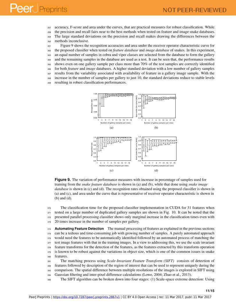
Create feature vector xs

Find similarity S f the

test and train features

Rank the global

similarity Sg to identify

unknown class m

Figure 6. The summary of the stages of proposed algorithm. The features are selected either manually

or through automatic extraction from the images. The image features are normalised using mean variance

filtering. The feature vectors are created with histograms of gradients and orientation of normalised

features. The resulting features are used in a min-distance classifier using a new product similarity metric.

6/15


Figure 7. The proposed maximum similarity template matching classifier with the product similarity.

Hart, 1967). They one of the simplest yet most powerful of the classifiers suitable for small sample175

problems (Raudys and Jain, 1990). The template matching can be illustrated as shown in the Fig 7. The176

main difference with the conventional minimum distance classifier is in the use of a new similarity metric177

that changes the minimum selector to a maximum selector. The ability of the classifier to correctly178

discriminate snake classes depends on the availability of inter-class discriminating features in the samples.179

We propose to ignore the missing features and calculate global similarity based on remaining features in a180

sample using a product based inter-feature similarity measure.181

Suppose xt(i) is the test sample and xg(i) is the gallery sample, and i represents the index of the ith

feature in the respective samples, then, the similarity S f (i) represents the similarity between the features:

S f (i) = xt(i)xg(i) (1)

The missing features in the feature vector xt is assigned a value 0 as this is indicative of the absence

or non-detection of the feature. Which means that the even if the there exists a numerical measure of

similarity between any missing features in xt and xg, the overall feature similarity S f would not have the

effect of missing features. The absence of a feature in a test would not result in similarity between the test

and gallery. The global similarity of a test sample with a class m containing J gallery samples with each

sample having N features can be represented as:

Sg(m) =N

∑i=1

(

1

J

J

∑j=1

S f ( j, i)

)

(2)

182

Suppose there are M classes and {cm1,cm2..,cmk} gallery samples per each class, then there will be

{cm1,cm2..,cmk} number of similarity values, Sg, for determining the class of the unknown test sample

xt . The class with the maximum number of high scores can be considered to be the most similar class to

which the test sample belongs. If m represents the class label, then the class of the unknown test sample

can be identified by:

m∗ = arg maxm

Sg(m) (3)

183

Implementation in CUDA184

Because the similarity S f is calculated at the feature level, and a global similarity Sg is calculated as an185

additive fusion of feature similarities at the class level, can be realised as a parallel processed algorithm in186

CUDA (Garland et al., 2008; Cook, 2012) as shown in Listing 1.187

188

__global__ void kernelProductSimilarity(float* j, float* Sf, float* Sm,189

int* indf, int featSize, int J)190

{191

//J=Total number of samples per class192

//Sf=Product similarity193

//Sm=Mean product similarity per feature in a class194

//featSize=Total number of features195

7/15


//j=Index of the gallery samples196

//indf=Index of the feature in a sample197

//x,y are coordinates of the two dimensional grid used for parallel198

computation199

unsigned int x = blockIdx.x*blockDim.x + threadIdx.x;200

unsigned int y = blockIdx.y*blockDim.y + threadIdx.y;201

Sm[y*featSize+x]=0;202

Sf[y*featSize+x]=0;203

indf[y*featSize+x]=0;204

for (j[y*featSize+ x]=1;j[y*featSize+ x]<J; j[y*featSize+x]++)205

{206

indf[y*featSize+x]=indf[y*featSize+x]207

+featSize;208

Sf[y*featSize+x]= Sf[y*featSize+x]+ feature_x[y*featSize+x]*209

feature_x[(y*featSize+x)+ indf[y*featSize+x]];210

}211

Sm[y*featSize+x]= Sf[y*featSize+x]/(J-1);212

}213214

Listing 1. Product similarity implemented as CUDA kernel code

The CUDA kernel code when tested for a similarity calculation on 10000 gallery samples with 31215

features and 10000 features has an execution time of 0.0013s and 0.14s, respectively. All the classification216

experiments reported in this paper is performed on Tesla 2070 GPU processor, and coding is done in C217

language.

Table 2. Example of proposed classification of snake data using 4 features

Features Local Similarity Global

Similarly

score

Class Sample F7 F12 F14 F1 S f (7) S f (12)S f (14)S f (1) Sg

Cobra1 0 1 0 1 0 1 0 1

1.52 0 1 0 0 0 1 0 0

Viper1 1 0 1 0 0 0 0 0

0.02 1 0 1 0 0 0 0 0

Unknown Xt 0 1 0 1 - - - - -

218

Classification with Feature Database219

The feature database consists of 31 taxonomically distinct observable snake features. The similarity220

calculation between the test and gallery is performed using S f . The global similarity Sg is calculated and221

the class of the sample under test is identified using m∗.222

0.0.1 Example on Feature Database223

Consider the example in Table 2, where two samples from each class (ie Cobra and Viper) is used as224

gallery xg while unknown sample xt is used as a test. To make the understanding clear, the xt originally225

belongs to the class Cobra. The task is to identify the class of the xt using the 4 example features F7, F12,226

F14 and F1.227

In this simple example, we calculate the local similarity S f (i) between the test and gallery features.228

Because the features F7 and F14 are absent in xt , it can be seen that they do not contribute to the positive229

similarity values of S f , which means that the global similarity Sg is formed of the local similarities from230

features F12 and F1. It can be seen that for the given example, the Viper class has a similarity score of 0.0231

against the Cobra class that has a similarity score of 1.5. The class of the test sample xt is identified as232

Cobra.233

Classification with Image Database234

The images in the gallery set can be used to create a template of features describing the snake. While

a feature sample based database can be used, a more practical approach in a real-time situation is to

have a technique that can automatically process the images directly for classification. Images are usually

affected by natural variabilities such as illumination, noise and occlusions. In order to reduce the natural

8/15


Figure 8. An example of the taxonomically identifiable feature F27 of cobra is shown in (a), and its

corresponding normalised orientation and magnitude histograms histn(θ) and histn(a) is shown in (b) and

(c), respectively.

variability, it is important to normalise the intensity values. The reduction in natural variability would

result in reduced intra-class image distances and improved classification accuracies. The image I can be

normalised using mean-variance moving window operation:

In(kx,ky) =∑

m1i=−m1 ∑

n1j=−n1

(

I(kx − i,ky − j)− Iµ

)

Iσ(4)

where, the window has a size of (2m+1)× (2n+1), Iµ is the mean and Iσ is the standard deviation of

the pixels in the image window. The normalised image In is converted into a feature vector, consisting

of orientation of gradients and magnitudes of the image pixel intensities. The gradient orientation θ

and magnitude a of In is computed at each point (kx,ky), given dy = In(kx,ky + 1)− In(kx,ky − 1) and

dx = In(kx +1,ky)− In(kx −1,ky) is calculated as:

θ(kx,ky) = arctan

(

dy

dx

)

(5)

and

a(kx,ky) =√

dx2 +dy2 (6)

The orientations θ is quantised in N bins of a histogram, and magnitude a is quantised into M bins of235

the histogram. The count of the histogram is normalised by dividing the counts in the individual bins236

by the overall area of the individual histograms. The normalised histograms histn(θ) and histn(a) is237

concatenated to obtain the feature vector for a snake image. An example of the normalised histogram238

features from the images are shown in Fig. 8.239

In the context of snake image database, we have a maximum of 31 feature images resulting from a

single sample of snake image. Suppose, I f is the normalised feature image, and histn(θ f ) and histn(a f )its corresponding orientation and magnitude features. Then, we can represent the overall fused feature

vector xs for any sample image s as:

xs = Ξ31i=1histn(θ f )Ξhistn(a f ) (7)

where Ξ represent the concatenation operator. The test images and gallery images are converted to feature240

vectors using xs.241

The similarity calculation between the test and gallery samples is performed, the global similarity Sg242

is calculated using Eq. 2 and the class of the sample under test is identified.243

RESULTS244

The feature database and image database of the snakes is used for analysing the classification performance245

of this two class small sample classification problem. The feature database contains 31 features, while246

image database consists of a total 1364 histogram features. Each of histn(θ) and histn(a) histogram247

feature consisted of 33 orientation features and 11 intensity features respectively, that resulted in a total of248

31×33×11 features. The experiments for classifier performance analysis were repeated 50 times by a249

random split for test and galley set to ensure statistical correctness.250

9/15


Table 3. Comparison of the proposed method with other classifiers when 5% of the class samples are

used as gallery and remaining 95% of sample are used as test on snake feature database.

Method % Correct F - Score AUC Precision (%) Recall (%)

Proposed 94.27± 6.34 0.959±0.062 0.937±0.005 92.11±14.4 93.03±10.4

J48(Quinlan,

1993)

90.00±6.70 0.922±0.057 0.914±0.007 97.17±6.7 88.25±8.3

IB1(Aha and Ki-

bler, 1991)

93.24±3.16 0.947±0.024 0.923±0.004 94.6±5.4 95.46±5.5

IBK(Aha and Ki-

bler, 1991)

93.49±3.20 0.949±0.024 0.933±0.004 94.61±5.4 95.86±5.3

LWL(Frank et al.,

2003)

92.42±5.34 0.940±0.045 0.919±0.060 94.78±5.7 93.75±7.0

RBF(Scholkopf

et al., 1997)

89.94±7.04 0.916±0.065 0.874±0.073 95.82±6.6 89.20±11.9

Voted Percep-

tron(Freund and

Schapire, 1998)

79.79±13.13 0.850±0.093 0.846±0.132 85.19±14.4 88.63±15.2

VF1(Demiroz and

Guvenir, 1997)

80.28±11.74 0.829±0.105 0.749±0.204 92.22±11.6 77.44±15.6

AdaBoost M1

(Freund and

Schapire, 1996)

90.50±6.71 0.921±0.057 0.914±0.072 97.11±6.8 88.25±8.3

Table 4. The performance of proposed classifier with other classifiers when 5% of the class samples are

used as gallery and remaining 95% of sample are used as test on snake image database

Method % Correct F - Score AUC Precision (%) Recall (%)

Proposed 85.20 ±7.10 0.91± 0.03 0.920 ± 0.06 89.95 ± 12.6 83.2±18.9

J48(Quinlan,

1993)

72.65±14.37 0.78±0.15 0.676±0.11 75.5±7.8 84.8±24.1

IBI(Aha and Ki-

bler, 1991)

81.21±5.29 0.86±0.04 0.762±0.06 81.3±5.2 93.3±9.9

IBK(Aha and Ki-

bler, 1991)

81.21±5.29 0.86±0.04 0.762±0.06 81.3±5.2 93.3±9.9

LWL(Frank et al.,

2003)

73.61±11.11 0.78±0.12 0.712±0.10 78.3±6.4 82.5±20.0

RBF(Scholkopf

et al., 1997)

84.08±7.43 0.89±0.06 0.823±0.09 88.0±6.5 91.8±11.7

Voted Percep-

tron(Freund and

Schapire, 1998)

71.65±8.28 0.80±0.06 0.772±0.08 74.8±10.3 90.8±14.1

VF1(Demiroz and

Guvenir, 1997)

83.40±8.25 0.86±0.07 0.911±0.05 89.1±6 85.3±12.6

AdaBoost

M1(Freund

and Schapire,

1996)

70.89±12.92 0.74±0.15 0.716±0.15 80.8±9.7 73.9±23.3

The samples in the database are randomly split into gallery and test, where 5% of total samples are251

used in the gallery while remaining 95% samples are used for the test. Table 3 and Table 4 shows the252

performance of the snake classifier problem using the presented product similarity classifier and several253

of the common classification methods. The performances indicated are percentage accuracy of correct254

classification, F-score value, the Area under the receiver operator characteristic curve, precision and recall255

rates. In comparison with other classifiers, the proposed classifier show performance improvements in256

10/15


accuracy, F-score and area under the curves, that are practical measures for robust classification. While257

the precision and recall fairs near to the best methods when tested on feature and image snake databases.258

The large standard deviations on the precision and recall makes drawing the differences between the259

methods inconclusive.260

Figure 9 shows the recognition accuracies and area under the receiver operator characteristic curve for261

the proposed classifier when tested on feature database and image database of snakes. In this experiment,262

an equal number of samples in cobra and viper classes are selected from the database to form the gallery263

and the remaining samples in the database are used as a test. It can be seen that, the performance results264

shows even on one gallery sample per class more than 70% of the test samples are correctly identified265

for both feature and image databases. A higher standard deviation with a low number of gallery samples266

results from the variability associated with availability of feature in a gallery image sample. With the267

increase in the number of samples per gallery to just 10, the standard deviations reduce to stable levels268

resulting in robust classification performances.269

(a) (b)

(c) (d)

Figure 9. The variation of performance measures with increase in percentage of samples used for

training from the snake feature database is shown in (a) and (b), while that done using snake image

database is shown in (c) and (d). The recognition rates obtained using the proposed classifier is shown in

(a) and (c), and area under the curve that is representative of receiver operator characteristic is shown in

(b) and (d).

The classification time for the proposed classifier implementation in CUDA for 31 features when270

tested on a large number of duplicated gallery samples are shown in Fig. 10. It can be noted that the271

presented parallel processing classifier shows only marginal increase in the classification times even with272

20 times increase in the number of samples per gallery.273

Automating Feature Detection The manual processing of features as explained in the previous sections274

can be a tedious and time-consuming job with growing number of samples. A purely automated approach275

would need the features to be automatically identified followed by an automated process of matching the276

test image features with that in the training images. In a view to addressing this, we use the scale invariant277

feature transforms for the detection of the features, as the features extracted by this transform operation278

is known to be robust against the variations in object size, which is one of the common issues in snake279

features.280

The matching process using Scale-Invariant Feature Transform (SIFT) consists of detection of281

features followed by description of the region of interest that can be used to represent uniquely during the282

comparison. The spatial difference between multiple resolutions of the images is explored in SIFT using283

Gaussian filtering and inter-pixel difference calculations (Lowe, 2004; Zhao et al., 2013).284

The SIFT algorithm can be broken down into four stages: (1) Scale-space extreme detection: Using285

11/15


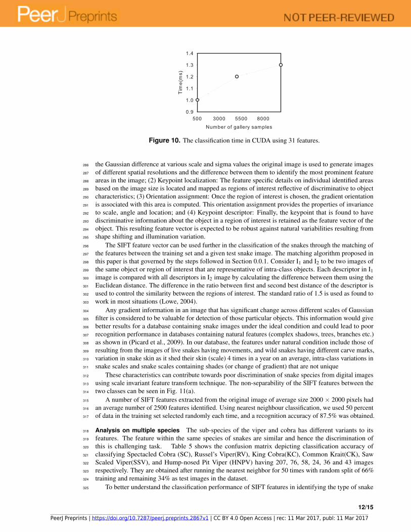
Figure 10. The classification time in CUDA using 31 features.

the Gaussian difference at various scale and sigma values the original image is used to generate images286

of different spatial resolutions and the difference between them to identify the most prominent feature287

areas in the image; (2) Keypoint localization: The feature specific details on individual identified areas288

based on the image size is located and mapped as regions of interest reflective of discriminative to object289

characteristics; (3) Orientation assignment: Once the region of interest is chosen, the gradient orientation290

is associated with this area is computed. This orientation assignment provides the properties of invariance291

to scale, angle and location; and (4) Keypoint descriptor: Finally, the keypoint that is found to have292

discriminative information about the object in a region of interest is retained as the feature vector of the293

object. This resulting feature vector is expected to be robust against natural variabilities resulting from294

shape shifting and illumination variation.295

The SIFT feature vector can be used further in the classification of the snakes through the matching of296

the features between the training set and a given test snake image. The matching algorithm proposed in297

this paper is that governed by the steps followed in Section 0.0.1. Consider I1 and I2 to be two images of298

the same object or region of interest that are representative of intra-class objects. Each descriptor in I1299

image is compared with all descriptors in I2 image by calculating the difference between them using the300

Euclidean distance. The difference in the ratio between first and second best distance of the descriptor is301

used to control the similarity between the regions of interest. The standard ratio of 1.5 is used as found to302

work in most situations (Lowe, 2004).303

Any gradient information in an image that has significant change across different scales of Gaussian304

filter is considered to be valuable for detection of those particular objects. This information would give305

better results for a database containing snake images under the ideal condition and could lead to poor306

recognition performance in databases containing natural features (complex shadows, trees, branches etc.)307

as shown in (Picard et al., 2009). In our database, the features under natural condition include those of308

resulting from the images of live snakes having movements, and wild snakes having different carve marks,309

variation in snake skin as it shed their skin (scale) 4 times in a year on an average, intra-class variations in310

snake scales and snake scales containing shades (or change of gradient) that are not unique311

These characteristics can contribute towards poor discrimination of snake species from digital images312

using scale invariant feature transform technique. The non-separability of the SIFT features between the313

two classes can be seen in Fig. 11(a).314

A number of SIFT features extracted from the original image of average size 2000 × 2000 pixels had315

an average number of 2500 features identified. Using nearest neighbour classification, we used 50 percent316

of data in the training set selected randomly each time, and a recognition accuracy of 87.5% was obtained.317

Analysis on multiple species The sub-species of the viper and cobra has different variants to its318

features. The feature within the same species of snakes are similar and hence the discrimination of319

this is challenging task. Table 5 shows the confusion matrix depicting classification accuracy of320

classifying Spectacled Cobra (SC), Russel’s Viper(RV), King Cobra(KC), Common Krait(CK), Saw321

Scaled Viper(SSV), and Hump-nosed Pit Viper (HNPV) having 207, 76, 58, 24, 36 and 43 images322

respectively. They are obtained after running the nearest neighbor for 50 times with random split of 66%323

training and remaining 34% as test images in the dataset.324

To better understand the classification performance of SIFT features in identifying the type of snake325

12/15


(a) (b)

Figure 11. (a)Number of SIFT features extracted from snake images. (b)The classification performance

of SIFT features for different percentage of training images.

Table 5. Confusion matrix on different types of snakes using SIFT.

Method SC RV KC CK SSV HNPV

SC 86.46 00.71 01.11 00.06 00.05 11.20

RV 06.15 66.00 06.46 00.00 00.15 21.23

KC 06.40 04.70 64.10 02.10 00.90 21.80

CK 05.00 06.00 13.00 58.75 08.75 08.50

SSV 16.67 02.33 03.83 07.00 51.00 19.17

HNPV 17.20 03.20 05.067 00.13 00.13 74.27

images, we varied the number of training and testing image used for classification. From Fig. 11(b) it can326

be seen that on the best accuracies for each sample size with increase in training samples per class the327

misclassified data reached to zero. It can also be noticed that the standard deviation is very less even in328

less number of training sample, proving that snake images of similar poses contribute to similarity match.329

From Fig. 12 shows that by varying the Euclidean distance ratio the number of features that get330

matched can be controlled. However, the classification of feature vectors obtained from SIFT technique331

can become a difficult task when the variability between the test and training samples are high. This332

makes the automated recognition of snakes in real-time imaging environments a challenging task.333

CONCLUSIONS334

In this paper, we demonstrated the use of taxonomy features in classification of snakes by developing335

a product similarity nearest neighbor classifier. Further, a database of snake images is collected, and336

converted to extract the taxonomy based feature and image snake database for our study.337

The knowledge base for the snake taxonomy can enhance the accuracy of information to administer338

correct medication and treatment in life threatening situation. The taxonomy based snake feature database339

can be used as a reference data for the classifier to utilize and compare the observations of the bite340

victim or the witness in realistic conditions. This can be further extended to other applications such341

(a) (b) (c) (d)

Figure 12. Matching SIFT feature descriptor by varying the distance measure in Nearest neighbour. (a)

ratio used is 0.7 and 11 features matched, (b) ratio used is 0.8 and 86 features matched, (c) ratio used is

0.85 and 225 features matched(a) ratio uses is 0.9 and 634 features matched.

13/15


as monitoring and preservation of snake population and diversity. The automatic classification using342

snake image database can help with the analysis of snake images captured remotely with minimal human343

intervention.344

There are several open problems that make snake recognition with images a challenging topic such345

as various natural variability and motion artefacts in realistic conditions. The automatic identification346

of snakes using taxonomy features offers better understanding of snake characteristics, and can provide347

insights into feature dependencies, distinctiveness and importance. The computerised analysis of snake348

taxonomy features can generate a wider interest between the computing specialist, taxonomist and medical349

professionals.350

ACKNOWLEDGMENTS351

The author would like to acknowledge Dileepkumar R, Centre for Venom Informatics, University of352

Kerala in the journey with the capture of images, and for providing the database required to conduct this353

computerized analysis. Balaji Balasubramanium of University of Nebraska - Lincoln, USA for initial354

assistance in this research work, and to my research assistants Bincy Mathews (now at Edge Technical355

Solution LLC) and Sherin Sugathan (now at Siemens Health-care) for their help in the organisation of the356

database.357

REFERENCES358

Aha, D. and Kibler, D. (1991). Instance-based learning algorithms. Machine Learning, 6:37–66.359

Aha, D. W., Kibler, D., and Albert, M. K. (1991). Instance-based learning algorithms. Machine Learning,360

6:37–66.361

Atkeson, C. G., Moore, A. W., and Schaal, S. (1997). Locally weighted learning. Artificial Intelligence362

review, 11:11–73.363

Bagui, S. C., Bagui, S., Pal, K., and Pal, N. R. (2003). Breast cancer detection using rank nearest neighbor364

classification rules. Pattern recognition, 36(1):25–34.365

Bailey, T. and Jain, A. (1978). A note on distance-weighted k-nearest neighbor rules. IEEE Transactions366

on Systems, Man, and Cybernetics, (4):311–313.367

Buhmann, M. D. (2003). Radial Basis Functions: Theory and Implementations. Cambridge University368

Press.369

Calvete, J. J., Juarez, P., and Sanz, L. (2007). Snake venomics. strategy and applications. Journal of Mass370

Spectrometry, 42(11):1405–1414.371

Cook, S. (2012). CUDA Programming: A Developer’s Guide to Parallel Computing with GPUs. Newnes.372

Cover, T. and Hart, P. (1967). Nearest neighbor pattern classification. IEEE transactions on information373

theory, 13(1):21–27.374

Demiroz, G. and Guvenir, H. A. (1997). Classification by voting feature intervals. In Machine Learning:375

ECML-97, pages 85–92. Springer Berlin Heidelberg.376

Demiroz, G. and Guvenir, H. A. (1997). Classification by voting feature intervals. In European Conference377

on Machine Learning, pages 85–92. Springer.378

Frank, E., Hall, M., and Pfahringer, B. (2003). Locally weighted naive bayes. In 19th Conference in379

Uncertainty in Artificial Intelligence, pages 249–256. Morgan Kaufmann.380

Freund, Y. and Schapire, R. E. (1996). Experiments with a new boosting algorithm. In Thirteenth381

International Conference on Machine Learning, pages 148–156, San Francisco. Morgan Kaufmann.382

Freund, Y. and Schapire, R. E. (1998). Large margin classification using the perceptron algorithm. In 11th383

Annual Conference on Computational Learning Theory, pages 209–217, New York, NY. ACM Press.384

Gao, Q.-B. and Wang, Z.-Z. (2007). Center-based nearest neighbor classifier. Pattern Recognition,385

40(1):346–349.386

Garland, M., Le Grand, S., Nickolls, J., Anderson, J., Hardwick, J., Morton, S., Phillips, E., Zhang, Y.,387

and Volkov, V. (2008). Parallel computing experiences with cuda. Micro, IEEE, 28(4):13–27.388

Gates, G. (1972). The reduced nearest neighbor rule (corresp.). IEEE Transactions on Information Theory,389

18(3):431–433.390

Gowda, K. and Krishna, G. (1979). The condensed nearest neighbor rule using the concept of mutual391

nearest neighborhood (corresp.). IEEE Transactions on Information Theory, 25(4):488–490.392

14/15


Guo, G., Wang, H., Bell, D., Bi, Y., and Greer, K. (2003). Knn model-based approach in classification. In393

OTM Confederated International Conferences” On the Move to Meaningful Internet Systems”, pages394

986–996. Springer.395

Halim, S. A., Ahmad, A., Md Noh, N., Mohd Ali, A., Hamid, A., Hamimah, N., Yusof, S. F. D., Osman,396

R., and Ahmad, R. (2012). A development of snake bite identification system (n’viter) using neuro-ga.397

In Information Technology in Medicine and Education (ITME), 2012 International Symposium on,398

volume 1, pages 490–494. IEEE.399

Halim, S. A., Ahmad, A., Noh, N., Md Ali Safudin, M., and Ahmad, R. (2011). A comparative study400

between standard back propagation and resilient propagation on snake identification accuracy. In IT in401

Medicine and Education (ITME), 2011 International Symposium on, volume 2, pages 242–246. IEEE.402

III, H. D. and Marcu, D. (2005). Learning as search optimization: Approximate large margin methods for403

structured prediction. In Proceedings of the 22nd international conference on Machine learning.404

Kotsiantis, S. B. (2007). Supervised machine learning: A review of classification techniques. In 2007405

conference on Emerging Artificial Intelligence Applications in Computer Engineering: Real Word AI406

Systems with Applications in eHealth, HCI, Information Retrieval and Pervasive Technologies, pages407

3–24.408

Li, S. Z., Chan, K. L., and Wang, C. (2000). Performance evaluation of the nearest feature line method in409

image classification and retrieval. IEEE Transactions on Pattern Analysis and Machine Intelligence,410

22(11):1335–1339.411

Liaw, Y.-C., Leou, M.-L., and Wu, C.-M. (2010). Fast exact k nearest neighbors search using an orthogonal412

search tree. Pattern Recognition, 43(6):2351–2358.413

Liu, T., Moore, A. W., and Gray, A. (2006). New algorithms for efficient high-dimensional nonparametric414

classification. Journal of Machine Learning Research, 7(Jun):1135–1158.415

Lowe, D. G. (2004). Distinctive image features from scale-invariant keypoints. International journal of416

computer vision, 60(2):91–110.417

McNames, J. (2001). A fast nearest-neighbor algorithm based on a principal axis search tree. IEEE418

Transactions on Pattern Analysis and Machine Intelligence, 23(9):964–976.419

Parvin, H., Alizadeh, H., and Minaei-Bidgoli, B. (2008). Mknn: Modified k-nearest neighbor. In420

Proceedings of the World Congress on Engineering and Computer Science, volume 1. Citeseer.421

Picard, D., Cord, M., and Valle, E. (2009). Study of sift descriptors for image matching based localization422

in urban street view context. In Proccedings of City Models, Roads and Traffic ISPRS Workshop, ser.423

CMRT, volume 9.424

Quinlan, R. (1993). C4.5: Programs for Machine Learning. Morgan Kaufmann Publishers, San Mateo,425

CA.426

Raudys, S. and Jain, A. (1990). Small sample size effects in statistical pattern recognition: recom-427

mendations for practitioners and open problems. In Pattern Recognition, 1990. Proceedings., 10th428

International Conference on, volume 1, pages 417–423. IEEE.429

Scholkopf, B., Sung, K.-K., Burges, C. J., Girosi, F., Niyogi, P., Poggio, T., and Vapnik, V. (1997).430

Comparing support vector machines with gaussian kernels to radial basis function classifiers. IEEE431

transactions on Signal Processing, 45(11):2758–2765.432

Sproull, R. F. (1991). Refinements to nearest-neighbor searching in k-dimensional trees. Algorithmica,433

6(1):579–589.434

Warrell, D. A. (1999). The clinical management of snake bites in the southeast asian region. Southeast435

Asian J Trop Med Public Health, (1). Suppl 1.436

Yong, Z., Youwen, L., and Shixiong, X. (2009). An improved knn text classification algorithm based on437

clustering. Journal of computers, 4(3):230–237.438

Zeng, Y., Yang, Y., and Zhao, L. (2009). Pseudo nearest neighbor rule for pattern classification. Expert439

Systems with Applications, 36(2):3587–3595.440

Zhao, W., Chen, X., Cheng, J., and Jiang, L. (2013). An application of scale-invariant feature transform441

in iris recognition. In Computer and Information Science (ICIS), 2013 IEEE/ACIS 12th International442

Conference on, pages 219–222. IEEE.443

Zheng, W., Zhao, L., and Zou, C. (2004). Locally nearest neighbor classifiers for pattern classification.444

Pattern recognition, 37(6):1307–1309.445

Zhou, Y., Zhang, C., and Wang, J. (2004). Tunable nearest neighbor classifier. In Joint Pattern Recognition446

Symposium, pages 204–211. Springer.447

15/15


Snake classification from images - PeerJ · Snake classification from images ... King Cobra, Common...

Documents

Transcript of Snake classification from images - PeerJ · Snake classification from images ... King Cobra, Common...