Smooth Transition Spatial Autoregressive Models · 2017-05-30 · Smooth Transition Spatial...

Smooth Transition Spatial Autoregressive Models

Bo Pieter Johannes Andree1,2,*, Francisco Blasques2,3, and Eric Koomen1

1Department of Spatial Economics/SPINlab, VU Amsterdam, Netherlands2Tinbergen Institute

3Department of Econometrics, VU University Amsterdam*Corresponding Author: email [email protected]

May 29, 2017

Abstract

This paper introduces a new model for spatial time series in which cross-sectional

dependence varies nonlinearly over space by means of smooth transitions. We refer

to our model as the Smooth Transition Spatial Autoregressive (ST-SAR). We estab-

lish consistency and asymptotic Gaussianity for the MLE under misspecification and

provide additional conditions for geometric ergodicity of the model. Simulation results

justify the use of limit theory in empirically relevant settings. The model is applied

to study spatio-temporal dynamics in two cases that differ in spatial and temporal ex-

tent. We study clustering in urban densities in a large number of neighborhoods in the

Netherlands over a 10-year period. We pay particular focus to the advantages of the

ST-SAR as an alternative to linear spatial models. In our second study, we apply the

ST-SAR to monthly long term interest rates of 15 European sovereigns over 25-year

period. We develop a strategy to assess financial stability across the Eurozone based on

attraction of individual sovereigns toward the common stochastic trend. Our estimates

reveal that stability attained a low during the Greek sovereign debt crisis, and that the

Eurozone has remained to struggle in attaining stability since the onset of the financial

crisis. The results suggest that the European Monetary System has not fully succeeded

in aligning the economies of Ireland, Portugal, Italy, Spain, and Greece with the rest

of the Eurozone, while attraction between other sovereigns has continued to increase.

In our applications linearity of spatial dependence is overwhelmingly rejected in terms

of model fit and forecast accuracy, estimates of control variables improve, and residual

correlation is better neutralized.

Keywords: Dynamic panel, Threshold models, Spatial heterogeneity, Spatial autocorrela-

tion, Urban density, Interest Rates, Monetary Stability, Sovereign Debt Crisis.

1

1 Introduction

Spatial entanglement of economic agents plays an important role in the realization of many

economic processes measured over space and time. Spatial autocorrelation models are

capable of describing the spatial dependence between variables measured across space and

are widely adopted in different research fields; see e.g. Kostov (2009) on agricultural land

prices, LeSage and Fischer (2008) on regional growth, Baltagi et al. (2014) on housing

prices, Hoshino (2016) with an application on crime data, and Debarsy et al. (2015) on

foreign direct investments.

Standard spatial models take into account spatial correlation in (un)observed variables,

but assume away the possibility of different spatial regimes. In particular, models that

allow for spatial (auto)correlation often do not sufficiently relax linearity constraints on

functional representations of spatial spillovers. Specifically, spillover-processes are repre-

sented by static “global” dependence parameters (Fotheringham, 2009). The literature

has stressed the importance of relying on local statistics for spatial dependence instead of

global measures due to parameter heterogeneity; see Anselin (1988), Anselin (1995) and

Fotheringham (2009).

Typically, spatial aggregation into grouped cross-sectional units relies on the use of

econometric tools that are helpful in avoiding ad-hoc sample divisions. Researchers have for

example relied on exploratory data analysis Baumont et al. (2006), Geographically Weighted

Regression (GWR) (Fotheringham et al., 2002; Su et al., 2012), boosted regression trees

(Crase et al., 2012), Bayesian (Glass et al., 2016), nonparametric (Frıas and Ruiz-Medina,

2016), or semiparametric (Basile et al., 2014) approaches to model heterogeneity.

All of the above approaches, however, treat the spatial dependence parameter as static.

Heterogeneity in interaction is achieved by using spatial trend surfaces or by sample divisions

that allow estimation of separate parameter vectors. For example, the Spatial Autoregres-

sive Semiparametric Geoadditive Models discussed by Basile et al. (2014) maintain linearity

assumptions with respect to the spatial autoregressive component, but have smooth locally

linear dependence structures through a spatial trend surface with respect to exogenous

variables.

The GWR approach is a recurring method in spatial econometric literature to model

spatial heterogeneity in coefficients. In this approach, neighborhoods are isolated in a Carte-

sian coordinate system using kernel density functions. Weighted parameter vectors are then

estimated for different neighborhoods. Numerous studies pointed out serious drawbacks of

this approach.1 Additionally, any trend surface strategy requires the entanglement structure

1Inadequate modeling of spatial lag and error processes (Leung et al., 2000a,b; Fotheringham et al., 2002;Paez et al., 2002a,b), spatial patterns revealed by GWR could be attributed to the procedure itself ratherthan the data generating process (Wheeler and Tiefelsdorf, 2005; Wheeler, 2007), and finally problems that

2

to be defined on a two-dimensional Cartesian coordinate system, which could be restrictive

for non-geographic weights matrix approaches.

In this paper we propose a parsimonious model that captures heterogeneity in spatial de-

pendence. The model builds on the well-known SAR model (Anselin, 1988) and the Smooth

Transition Autoregressive (STAR) framework advocated by Granger and Terasvirta (1993)

and Terasvirta and Anderson (1992); Terasvirta (1994). The model allows for the possi-

bility of regime-specific dynamics in spillovers and allows for detection of spatial regimes

with differential in intensity of spatial spillovers. Feedback loops that amplify spillovers

in the cross-section are modeled in this way with varying intensity. The regime-specific

dynamics in the cross-sectional dimension are driven by a smooth transition function. The

entanglement structure remains exogenously determined through the specification of a spa-

tial weights matrix following standard procedures in the spatial econometric literature.

The method provides an attractive alternative to other methods designed to capture cross-

sectional heterogeneity like the GWR, or models that feature grouped patterns based on

fixed-effects. We point out that our method does not depend on spatial trend surfaces and

can without difficulty be applied in settings where cross-sectional linkages are based on a

broad class of distance metrics.

We establish the asymptotic properties of the intractable Maximum Likelihood Esti-

mator (MLE) for all static parameters. Our asymptotic results allow for possible model

misspecification. We focus on t-distributed errors as a generalization of Gaussian distur-

bances and as an attractive way to achieve robustness to outliers or estimate fat-tailed

processes. Additional results regarding the ergodicity of data generated by the model are

also provided.

We discuss identification of the parameters of the time-varying MLE and the implications

for nonlinearity tests based on the Information matrix. As an alternative to Wald-type tests,

we explore model selection procedures based on information criteria following Granger et al.

(1995); Sin and White (1996). Evidence from the simulation study suggests that we can rule

out linear dependence and justify inference on the parameters of the MLE for empirically

relevant sample sizes. The simulations also show that the framework is robust to overfitting

of additive outliers. False selection rates decrease with sample size but we do not attain a

zero false selection rate.

We apply our model empirically in two case studies with different panel dimensions. In

the first application, we study dynamics in local residential density in the Netherlands over

relate to bandwidth selection and local violations of least-squares assumptions (Wheeler and Tiefelsdorf,2005; Farber and Paez, 2007; Cho et al., 2010). We note that grouping observations not by kernels butthrough fixed effect approaches also has its drawbacks because convergence rates depend on the number ofobservations in groups tending to infinity (Bonhomme and Manresa, 2015), while in many practical situationsadditional observations can only be collected over time with group sizes remaining fixed.

3

the period 2005 to 2014. The data set consists of a large N and small T panel. We test two

hypotheses regarding cross-sectional dependence structures that cannot be captured using

linear models: (i) that spatial autoregressive properties should be a magnitude stronger in

cities and decay outwards in line with the distance decay of agglomeration effects (Fother-

ingham, 1981); and (ii) that the relation between urban densities and average household

composition in surrounding neighborhoods should vary across the urban gradient, reflecting

sorting patterns that arise under single-crossing assumptions about household preferences

(Epple and Sieg, 1999). We model nonlinearities in both dependence structures with a

threshold function specified around population densities and find strong evidence for both

hypotheses.

Our second application is on monthly long term interest rates of 15 European sovereigns

over the period 1994-2015. This data set consists of a small N and large T panel. We study

the dynamics of endogenously driven contraction toward a common stochastic trend in an

integrated network of sovereigns. We pay particular focus on the time-varying properties

of local spatial contraction parameters and develop a strategy to assess financial stability.

Our spatial weights matrix is based on pair-wise correlations and allows entanglement of

areas that are distant from each other from a spatial perspective. This weights matrix

specification allows for differential in centrality of the different sovereigns within the spillover

network. We explore the dependence structure in the context of an ARMA process, and

test several specifications for the nonlinear spatial process based on a mix of the AR and

MA components.

In both applications, the results are in overwhelming support of threshold nonlinearities

in the spatial dependence parameters. We show that the nonlinear model is able to deliver

better in- and out-of-sample forecasts and that the nonlinearities are robust to a wide range

of model specifications.

The remainder of this paper is organized as follows. Section 2 considers spatial autocor-

relation models and proposes our new framework to capture nonlinear spatial dependencies.

Estimation theory for the MLE is examined in Section 3. Section 4 confronts the large sam-

ple theory to empirically relevant settings and provides the results of our simulation study.

Specifically, we look at the small sample distributions of the MLE and selection frequen-

cies of correctly- and misspecified models. We simulate under innovations drawn from a

fat-tailed distribution and explore the impact of additive outliers. The model is applied in

Section 5 where we provide results for our analyses on Dutch urban densities and financial

stability across the Eurozone. Section 6 summarizes and concludes. Finally, additional

results and proofs for our main Theorems are located in Appendix A.

4

2 Linear and Nonlinear Spatial Autoregressive Models

2.1 Linear Dynamics: The SAR Model

Spatial data is often highly dependent across space. In order to model this dependence,

Cliff and Ord (1969) proposed the Spatial Autoregressive (SAR) model. The SAR in the

context an Autoregressive Moving Average model with Exogenous Regressors (ARMAX)

model is given by:2

Yt = ρWYt + Yt−pφ+Xtβ + εt + εt−qµ ∀ t ∈ Z , (1)

εtt∈Z ∼ pε(εt,Σ, λ) ,

where Yt denotes a vector of n cross-sectional observations at time t, ρ is the spatial depen-

dence parameter, W is the n × n matrix of exogenous spatial weights, φ is a p × 1 vector

of autoregressive components, Xt is an n× (k + 1) matrix of k exogenous regressors plus a

unit vector, β is a (k + 1)× 1 vector of k coefficients plus an intercept, µ is a q × 1 vector

of MA components and εt is the disturbance vector with multivariate density pε(εt,Σ, λ)

with zero mean and an unknown k× k scalar variance-covariance matrix Σ. Other possible

parameters are contained in vector λ.

In this model structure, each observation of yit in the vector Yt depends on k individual

specific regressors xit,kKk=1T

t=1, as well as the entries of xjt,kKk=1T

t=1 for i 6= j. For a

sufficient amount of observations n, such a system cannot be estimated without imposing

further restrictions. Spatial dependence modeling is made operational by specifying the

spatial weights matrix W as an exogenous function of some relevant normed vector space,

for example a function of geographic distances, thereby defining exogenously the structure

between cross-sectional entries.

It is standard procedure to row-normalize W such thatn∑j=1

wij = 1 ∀ i ∈ n, where wij

is the i,j-th element from W . The parameter ρ captures the spatially weighted effects of

neighboring values WYt on Yt. In this simple framework, nonlinear feedback effects across

entries can be captured, shown by rewriting the model as:

Yt = H−1(Yt−pφ+Xtβ + εt + εt−qµ), (2)

εtt∈Z ∼ N ID(0, σ2ε),

2Anselin (1988) argues that spatial heterogeneity can further complicated the analysis. His argument iscentered on the notion that geographic phenomena often do not deviate around a constant mean, but likelymove from one local average to another. For this reason, the simple SAR model may be a problematic modelfor describing the very phenomenon that Cliff and Ord (1969) are trying to model; see Fotheringham (2009)for a discussion.

5

where H := In − ρW and In denotes the n × n identity matrix. Following LeSage (2008)

we obtain the following infinite power series expansion

Yt = (In + ρ1:∞W 1:∞)(Yt−pφ+Xtβ + εt + εt−qµ), (3)

with ρ1:∞W 1:∞V = V + ρWV + ρ2W 2V + ...+, for an arbitrary vector V . Equation (3)

reveals that the entire ARMAX structure spills over to other regions j 6= i with a rate

that declines as proximity to i increases, via the structure imposed by W . Feedback effects

occur for positive wij and wji and mutual neighbours i and j, as by construction of the

spatial weights matrix W , every observation is a second order neighbour of itself. A stable

process therefore requires exogenous shocks to die out over space, which for the linear spatial

process is guaranteed if ρ ∈ [1/ωmin, 1/ωmax], where ωmin is the smallest eigenvalue of W

(Lee, 2004), or equivalently |ρ| < 1, if the rows of W sum up to one.

The endogenous nature of this model causes inconsistencies in the least squares estimator

that increase with n. However, we can consistently estimate the system by Quasi Maximum

Likelihood methods (Q)ML or Generalized Methods of Moments (GMM), e.g. Kelejian and

Prucha (2010). ML estimation of spatial models with static spatial parameters is pioneered

in Ord (1975) and the asymptotics of the QML estimator are derived in Lee (2004). Finite

sample distributions are investigated by Das et al. (2003); Bao and Ullah (2007).

2.2 The Smooth Transition Spatial Autoregressive Model

The linearity of the SAR model imposes the crucial simplifying assumption that the spatial

dependence is fixed for any levels of both Yt andXt. As we shall see in Section 5 however, this

linearity assumption is not supported by the data. Evidence of nonlinear spatial dependence

seems pervasive in economic applications.

In what follows we allow the spatial dependence parameter ρ to change as a function of

a vector of variables Zt that may include (spatial lags of) Yt−p or εt−q for any (p, q) ≥ 1

and or Xt. In particular, we build on the popular smooth transition autoregressive (STAR)

model introduced in Terasvirta and Anderson (1992); Terasvirta (1994).3 The resulting

Smooth Transition Spatial Autoregressive (ST-SAR) model with ARMAX terms takes the

form4

Yt = ρ(θρ;Zt) WYt + Yt−pφ+Xtβ + εt + εt−qµ, (4)

3The STAR model is well known in the time-series literature for modeling nonlinear dynamics withthresholds; see Granger and Terasvirta (1993) for a literature review of nonlinear time-series models. For acomprehensive review of STAR models, the reader is referred to Dijk et al. (2002).

4We discuss the nonlinear model within an ARMAX framework because, as we shall see in our applica-tions, all of terms can affect the data both directly and through the spatial dependence parameters. Allowingthe terms to explicitly effect Yt directly and through ρ(θρ;Zt) simultaneously, is crucial to determine throughwhich channel the effects move.

6

εtt∈Z ∼ pε(εt,Σ, λ),

where the spatial dependence ρ(θρ;Zt) is determined by

ρ(θρ;Zt) = κ+δ

1 + exp(−γ(Zt − τ(θτ ;Zt))), (5)

and τ(θτ ;Zt) = α+ Ztϕ, (6)

where denotes element-by-row multiplication, θρ denotes the vector of unknown parame-

ters θρ := (κ, δ, γ, θτ ), and θτ := (α,ϕ) is a parameter vector of possible additional param-

eters within the threshold function that may include linear coefficients w.r.t. any of the

ARMAX terms contained in Zt.

The quantity Zt − τ(θτ ;Zt) measures deviations of Zt from a possibly time-varying

quantity τ(θτ ;Zt). In general, we allow τ(θτ ;Zt) to be any function of the data Zt. In this

paper we consider first order polynomials around three important alternatives, the cross-

sectional average τ(θτ ;Zt) = α + ϕn−1∑n

i=1 zit, the local average τ(θτ ;Zt) = α + ϕWZt,

and local observations τ(θτ ;Zt) = α + Ztϕ. Other options include modeling τ(θτ ;Zt) as a

constant α only, or using regional averages WlZt with Wl as a spatial weights matrix that

includes up to l higher order spatial lags.

Note that Equation (5)-Equation (6) allow the spatial dependence to change smoothly

between regimes. The ST-SAR model differs considerably from time-varying spatial pa-

rameter models such as the spatial score model proposed in Blasques et al. (2016) which

attempts to filter the unobserved time-varying sequence ρtt∈Z by means of a score fil-

ter. The nonlinear STAR formulation explores the relation between the spatial dependence

parameter ρ and variables in Zt. In particular, the parameters δ, τ(θτ ;Zt) and γ pro-

duce dynamics that cannot be reproduced by the time-varying spatial parameter model

ofBlasques et al. (2016). It is also worth noting that the STAR dynamics nest not only the

linear SAR model of Cliff and Ord (1969), but also, a threshold model (like the TAR model

Tong (1978); Tsay (1989); Tong (2015)) with instantaneous switching function between two

regimes. The linear SAR case is obtained when γ → 0. In contrast, a threshold switching

model is obtained when γ → ∞. Depending on Zt, the transition mechanism may be en-

dogenous or exogenous in nature. In the empirical section we shall consider both exogenous

cases such as Zt = Xt and endogenous examples where we allow the nonlinearities to be

driven by ARMA terms.

Finally, we note that, just as in the case of the SAR model, the ST-SAR can also be

re-written as

Yt = H(θρ;Zt)−1(Yt−pφ+Xtβ + εt + εt−qµ) (7)

where H(θρ;Zt) := In − ρ(θρ;Zt) W .

7

3 Asymptotic theory for the ST-SAR Model

Estimation of the ST-SAR model’s parameters is crucial to infer if nonlinear dynamics are

present in the data. The estimated parameters will also inform us about the existence

of threshold dynamics, the location of those thresholds, and the smoothness and speed of

transitions. In this section we present and discuss the properties of both the log likelihood

function and the ML estimator. We further provide conditions for the existence, strong

consistency and asymptotic normality of the MLE for all parameters that define the ST-

SAR. Proofs can be found in Appendix A. Our asymptotic results all refer to increasing

the time dimension rather than the spatial dimension since the applications we consider are

such that N cannot grow. Additional observations are collected over time only.

Let θ denote the vector of parameters of our ST-SAR model, θ := (θy, θρ), θτ ∈ θρ,

θ := (β, φ, µ, κ, δ, γ, α, ϕ)′. Furthermore, let θ0 denote the parameter of interest. Naturally,

the ML estimator θT is defined as

θT ∈ arg maxθ∈Θ

T∑t=1

`t(θ), (8)

where

`t(θ) = ln detH(θρ;Zt) + ln pε(H(θρ;Zt)Yt − Yt−pφ−Xtβ − εt−qµ,Σ;λ). (9)

The dependence of `t(θ) on the data is omitted in the notation for convenience. Equa-

tion (9) differs from a standard cross-section likelihood function by the log determinant

ln detH(θρ;Zt), which accounts for the nonlinear spatial feedback (Anselin, 1988). Note

that εt−q is unobserved and naturally a function of past observed data, with the initial

vectors set at zero. In this paper we shall focus on innovations with density pε given by

the multivariate Student’s t-distribution. The t-distribution naturally generalizes the mul-

tivariate normal distribution to allow for fat tails, rendering the dynamics more robust to

incidental outliers. Using the standard expression for the multivariate t-distribution with

λ degrees of freedom we obtain

`t(θ) = Q(θρ;Zt) +A(θ) +−1

2(λ+ n)F (θ, Yt, Xt, Zt),

where Q(θρ;Zt) is the log determinant

Q(θρ;Zt) := ln detH(θρ;Zt),

8

A(θ) is a constant given by

A(θ) := ln Γ ((λ+ n)/2)[detΣ

12 (λπ)

n2 Γ (λ/2)

]−1,

and the random element F (θ, Yt, Xt, Zt) is naturally defined as

F (θ, Yt, Xt, Zt) :=

ln(

1 + λ−1(H(θρ;Zt)Yt − φYt−1 −Xtβ − µεt−1)′Σ−1(H(θρ;Zt)Yt − φYt−1 −Xtβ − µεt−1)).

We first establish the existence and measurability of the MLE θT . This ensures that the

arg max set in Equation (8) is not empty and that θT is a random variable.

Assumption 1 (Compactness of Θ). (Θ,B(Θ)) is a measurable space and Θ is a compact

subset of Rdθ .

Theorem 1 (Existence and Measurability). Let Assumption 1 hold. Then there exists a.s.

an F/B(Θ)-measurable map θT : Ω→ Θ satisfying Equation (4) for all T ∈ N.

Consistency of the MLE θT w.r.t. the parameter of interest θ0 ∈ Θ can be obtained under

standard regularity conditions. Assumptions 2-3 impose the SE nature of the data and

a bounded moment for Q(θρ;Zt) and F (θ, Yt, Xt, Zt). Assumption 4 ensures that θ0 is

identified.

Assumption 2. The random sequence Yt, Xtt∈Z is SE.

Assumption 3. The following moment conditions are satisfied:

i E supθ∈Θ |Q(θρ;Zt)| <∞;

ii E supθ∈Θ |F (θ, Yt, Xt, Zt)| <∞.

Assumption 4. θ0 ∈ Θ is the unique maximizer of the limit likelihood; i.e. E`t(θ0) >

E`t(θ) ∀ (θ, θ0) ∈ Θ×Θ : θ 6= θ0.

Theorem 2 below establishes the strong consistency of the MLE θT with respect to θ0 ∈ Θ.

The moment condition E supθ∈Θ |Q(θρ;Zt)| < ∞ in Assumption 3 is implied by positive

definiteness of detH(θρ;Zt)−1 which for the SAR with a row-normalized W follows from

|ρ| < 1. We note that the nonlinear case this is markedly different, and |ρ(θρ;Zt)| < 1 is

not a required condition for E supθ∈Θ |Q(θρ;Zt)| <∞; see Lemma 3 in the Supplementary

Appendix.

Theorem 2 (Strong consistency). Let Assumptions 1-4 hold. Furthermore, let Θ be such

that Σ is positive definite for every θ ∈ Θ. Then the MLE satisfies θTa.s.−−→ θ0 as T →∞.

9

Theorem 2 shows that the MLE converges almost surely to θ0 as the sample size increases

in the time dimension. When the model is well specified, θ0 corresponds naturally to

the so-called true parameter that indexes the distribution of the data. If the model is

misspecified, then θ0 is often called a pseudo-true parameter that, by construction, is the

minimizer of the Kullback-Leibler divergence (Kullback and Leibler, 1951) between the true

conditional probability of the data and the conditional distribution implied by the ST-SAR

model; see e.g. White (1994a) for details. In this sense, under model misspecification, the

MLE converges at least to the parameter that delivers the best approximation to the true

distribution of the data.

Theorem 3 below obtains the asymptotic normality of the MLE by application of

Billingsley’s central limit theorem (CLT) for an SE martingale difference sequence (mds);

see Billingsley (1961). Assumption 5 imposes the mds property. This assumption is ap-

propriate if the model is reasonably well specified. In effect, if the model is well specified,

then the score is a mds by construction. This is not the case, however, under strong model

misspecification; see White (1994a).5

Assumption 5. The score ∇`t(θ0)t∈Z is a mds.

Assumption 6 imposes additional moment conditions that ensure the application of a CLT to

the score and a uniform law of large numbers to the second derivative of the log likelihood

function. Below we let ∇iQ(θρ0;Zt) and ∇iF (θ0, Yt, Xt, Zt) denote the ith derivative of

Q(θρ0;Zt) and F (θ0, Yt, Xt, Zt) with respect to the vector θ. The moment conditions are

imposed on each element of the resulting vectors and matrices.

Assumption 6. The following moment conditions are satisfied:

(i) E|∇Q(θρ0;Zt)|2 <∞;

(ii) E|∇F (θ0, Yt, Xt, Zt)|2 <∞;

(iii) E supθ∈Θ |∇2Q(θρ0;Zt)| <∞;

(iv) E supθ∈Θ |∇2F (θ0, Yt, Xt, Zt)| <∞.

Theorem 3 delivers the asymptotic Gaussianity of the standardized MLE by imposing the

further regularity condition that θ0 lies in the interior of the parameter space int(Θ).

Theorem 3 (Asymptotic Normality). Let assumptions 1-6 hold with Σ positive definite for

every θ ∈ Θ. If θ0 ∈ int(Θ), then the MLE satisfies

5Under strong model misspecification, the asymptotic Gaussianity of the score may still be obtained,under appropriate regularity conditions, by application of a central limit for processes that are near epochdependent or Lp approximable by a mixing process; see e.g. Potscher and Prucha (1997).

10

√T (θ − θ0)

d−→ N(0, I−1(θ0)J (θ0)I−1(θ0)

)as T →∞,

where J (θ0) := E`′t(θ0)`′t(θ0)ᵀ is the expectation of the outer product of the score, and

I−1(θ0) := −E`′′t (θ0) denotes the Fisher information matrix.

A theory of estimation and inference under correct-specification usually requires a study

of the model as a data generating process. We provide additional results regarding the

geometric ergodicity of data generated by the ST-SAR in the Supplementary Appendix. As

we shall see, the Monte Carlo simulation developed in Section 4 provides evidence of both

the consistency and normality claims made in Theorem 2 and Theorem 3 in the correct

and misspecified case. Most importantly, the asymptotic Gaussian distribution seems to

provide a good approximation for the finite sample distribution of the MLE in empirically

relevant sample sizes.

4 Monte Carlo study

To evaluate the adequacy of the ST-SAR framework in fitting dynamic spatial correlation

patterns, we conduct a Monte Carlo study. In our first experiment, we investigate whether

the MLE is well-behaved and approximately normal for increasing sample sizes. In our

second study we investigate model selection based on standard information criteria. To

limit the complexity of the experiment, we consider a spatial autoregressive process without

exogenous regressors and focus on a model with Student-t innovations. The data generating

process is:

Yt = H(θρ;Yt−1)−1(εt), εt ∼ TID(1, In; 5), (10)

with ρ(θρ;Yt−1) as layed out in Equations (5) to (6). In our first experiment we set the

parameters values to

δ = 1.35, γ = 1.05, α = −0.2, ϕ = 1.4, κ = −0.4, Zt = Yt−1, τ(θτ ;Zt) = α +

ϕ/N∑N

1 (Yt−1).

The data generating process satisfies the conditions for geometric ergodicity with spatial

dependence parameters taking values in |ρ(θρ;Yt−1)| ∈ [0, 0.95] and allows for local positive

and negative clustering, see Appendix A.3.

We keep the ratio of distant and close-by neighbors comparable across experiments

by allowing the network density of the weights matrix to increase with N . In each draw

we generate a random zero diagonal row-normalized weights matrix with N/10 neighbors

for each observation. The process is initialized with H1 = In, and the first 50 steps of the

sequence are discarded to avoid dependence on the initialization. We simulate 1000 datasets

according to Equation (10) and estimate the parameters of the ST-SAR with λ ,σ and a

11

constant as free parameters. We consider samples of size T = 25, 100, 250 for N = 30, 60.

It is well-known that the small sample behavior of the MLE depends both on the degree

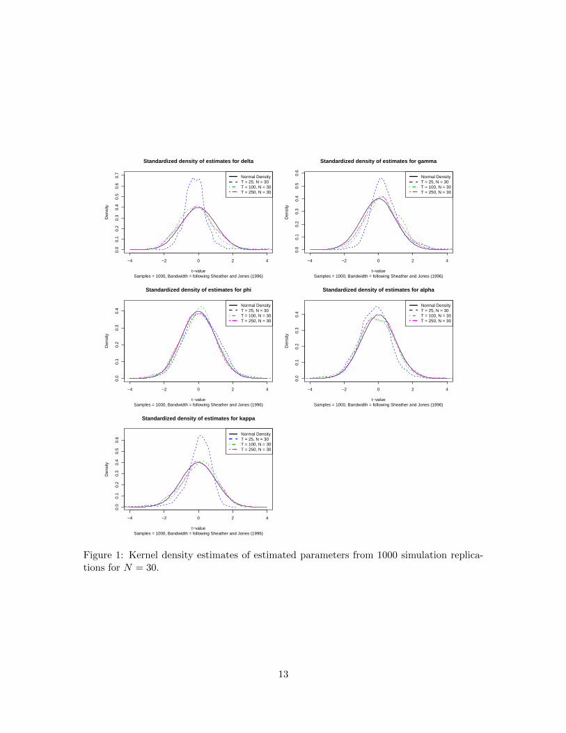
of sparseness of the weights matrix and the sample size (Bao and Ullah, 2007). Figure 1

presents kernel density estimates of the distribution of the MLE for the different sample

sizes.

Figure 1 presents the results for N = 30, and shows clearly that for small sample sizes

the estimators are not perfectly normal. For larger sample sizes, we see a fast convergence

towards the limiting result. The Appendix includes the distributions for N = 60. The

results indicate that for an empirically relevant signal and sample size the MLE is well-

behaved.

Note however that the results do not directly generalize to any empirical setting. Specif-

ically, stronger signals may be estimated appropriately at smaller sample sizes while weaker

signals might cause identification problems even in larger samples. We therefore extend our

numerical investigation by focussing on selection frequencies based on standard information

criteria as a more robust way to conclude on the significance of estimated nonlinearities. We

simulate from a weaker dependence signal, and focus on a process driven by local averages

to cover the model in a variety of settings. Additionally, the local average should be more

severely distorted by additive outliers. We simulate using the following specification:

1 δ = 0.4, γ = 1.05, α = −0.2, ϕ = 1.4, κ = −0.4, Zt = Yt−1, τ(θτ ;Zt) = α+ϕWYt−1,

2 SAR with ρ = 0.5.

We estimate parameters for two versions of the ST-SAR; (i) a parsimonious specification in

which the threshold is modeled as constant and the constant spatial dependence component

is omitted (ϕ and κ are fixed at 0); and (ii) the correctly specified ST-SAR with all its

parameters. We focus on selection between linear and nonlinear models and between the

two different nonlinear specifications.

We provide results for the Akaike’s information criterion (AIC), the corrected AIC

(AICc), and a modified AIC (mAIC). Under well known conditions, the AIC proposed in

Akaike (1973, 1974) provides a consistent ranking of models based on the Kullback-Leibler

divergence between the true distribution of the data and the model-implied distribution.

The AICc, introduced by Hurvich and Tsai (1989), improves on the finite sample properties

of the AIC; see Brockwell and Davis (1991), McQuarrie (1998) and Burnham and Anderson

(2004). The mAIC used here is based on the more general setting put forward by Sin and

White (1996).

In this study we also consider the effect of additive outliers, similar to Dijk et al. (1999),

12

−4 −2 0 2 4

0.0

0.1

0.2

0.3

0.4

0.5

0.6

0.7

Standardized density of estimates for delta

Samples = 1000, Bandwidth = following Sheather and Jones (1996)t−value

Den

sity

Normal DensityT = 25, N = 30T = 100, N = 30T = 250, N = 30

−4 −2 0 2 4

0.0

0.1

0.2

0.3

0.4

0.5

0.6

Standardized density of estimates for gamma


Den

sity


−4 −2 0 2 4

0.0

0.1

0.2

0.3

0.4

Standardized density of estimates for phi


Den

sity


−4 −2 0 2 4

0.0

0.1

0.2

0.3

0.4

Standardized density of estimates for alpha


Den

sity


−4 −2 0 2 4

0.0

0.1

0.2

0.3

0.4

0.5

0.6

Standardized density of estimates for kappa


Den

sity


Figure 1: Kernel density estimates of estimated parameters from 1000 simulation replica-tions for N = 30.

13

Table 1: Selection frequencies for data generated from the ST-SAR.

ST-SAR DGPST-SAR 1vs. SAR

ST-SAR 2vs. SAR

ST-SAR 2vs. ST-SAR 1

AIC AICc mAIC AIC AICc mAIC AIC AICc mAIC

N=30 T=10 38 38 38 45 41 43 46 45 46T=25 62 61 62 63 62 63 50 48 49T=50 80 79 80 83 82 82 57 57 57T=100 85 85 85 97 97 97 80 80 80T=250 100 100 100 100 100 100 96 96 96

N=40 T=10 51 49 50 52 50 51 44 43 44T=25 72 72 72 73 72 72 51 50 50T=50 93 93 93 91 91 91 59 59 59T=100 92 92 92 100 100 100 84 84 84T=250 100 100 100 100 100 100 99 99 99

N=50 T=10 53 52 53 54 52 53 45 43 45T=25 84 84 84 85 84 85 55 55 55T=50 98 98 98 98 98 98 66 66 66T=100 99 99 99 100 100 100 89 89 89T=250 100 100 100 100 100 100 100 100 100

N=60 T=10 63 62 63 59 58 59 45 43 44T=25 88 88 88 87 87 87 57 56 57T=50 99 99 99 99 99 99 71 71 71T=100 99 99 99 100 100 100 92 92 92T=250 100 100 100 100 100 100 100 100 100

by simulating contaminated sequences according to the following replacement process:

ζt = Yt + 1.[µt > 0.5]ψεt, (11)

µt ∼ UID(0, In),

εt ∼ BID(−In, In;π),

with π = 0.05 and ψ set to the sample equivalents of√EY 2

t − (EYt)2, and ζt entering the

likelihood function.

The results show that both the parsimonious and correctly-specified descriptions of the

data are selected over the SAR with increasing frequency as the sample size increases.

The parsimonious model seems to fit an important part of the nonlinear process generated

under the larger parameter space. When the correctly-specified model is pitted against the

parsimonious model, we see that the selection frequency stays moderate for T ≤ 50, after

which it increases rapidly. In large samples the additional information captured by κ and

ϕ is decisive in selecting the correct specification with probability 1.

Table 7 in the Appendix provides results for the contaminated process. Overall, the

14

presence of additive outliers has only a small effect. For T = 10 we observe some increase

in power, though for T > 10 the outliers seem to negatively impact power. Especially

the selection frequencies of the correct model seem to go down when pitted against the

parsimonious model. While we reach a frequency of 92% for (N,T ) = (60, 100) without

contamination, we obtain a weaker selection rate of 80% percent for data distorted by

outliers. The reduction in power is somewhat contrary to the univariate framework in which

additive outliers are known to sometimes trick the threshold into fitting the contamination

incorrectly as a nonlinear process (Dijk et al., 1999). We find that in the cross-sectional

case, the results mirror what can be expected in simple linear regression models.

Table 8 provides results for data simulated from the SAR. We narrow our focus to setting

the correctly-specified model against the SAR. The results show that the SAR is correctly

selected, with increasing probability as sample size grows, over the nonlinear model when

the data generating process is in fact linear. Hence, the evidence is in line with the theorized

convergence toward zero of false selection probabilities of the nonlinear model, though we

do not reach zero even at N = 60 and T = 250. At our largest samples, we still maintain

around 17 percent false selections. Therefore, one should be careful in interpreting results

when the difference in information criteria is small. In our empirical applications however,

we find that the difference in information is overwhelming with little room left for chance.

Finally, contamination of the linear process does not seem to increase false selection rates.

The study reveals that for empirically relevant sample sizes the MLE is well-behaved and

approximately Gaussian. Simulations confirm the appropriateness of standard information

criteria that offer different descriptions of spatial spillover processes. The AICc comes

forward as the most conservative measure, and therefore we apply it as our primary choice

criterion in the empirical section.

5 The empirics of nonlinear spatial dependencies

In our empirical study we present two cases. In our first study we use a panel of short T

and large N . We evaluate nonlinear spatial dynamics in the clustering of Dutch residential

densities at the neighborhood level over a period of ten years. The primary focus is on

the advantages of the ST-SAR compared to its linear counterpart. We investigate spatially

varying features of the dependence structure, particularly in relation to a number of spa-

tially explicit socio-economic variables. The application shows that the ST-SAR is able to

fit heterogeneous relationships that the SAR fails to describe. This added flexibility is over-

whelmingly favored by information criteria and forecast accuracy measures, and improves

the estimates of the impact of exogenous regressors.

The second application tracks monthly long term interest rates for across an integrated

15

network of 15 European sovereigns over a period of 23 years, and explores the ST-SAR in the

context of large T and small N . The dataset includes observations from before the European

Union, during the expansion of the EU, the Great Recession, and the Greek sovereign

debt crisis. We develop a strategy to evaluate financial stability by analyzing variation in

contraction toward a common trend across the Eurozone. We model contraction in the

cross-section with a time-varying threshold function driven by an ARMA specification, and

explore convergence and dispersion between rates of different sovereigns over the entire time

span. In this application we primarily seek to better understand the temporal dynamics, and

show that evidence of nonlinearity is not only pervasive in a sense of statistical significance,

but that the estimated dynamics also provide a meaningful description of the economic

process.

5.1 Dutch residential densities

5.1.1 Data

Residential density data

The Netherlands is one of the most densely populated country in the world. Dutch cities are

however relatively small (the largest city has less than one million inhabitants), and popula-

tion is fairly dispersed in a polycentric network of smaller cores. The sample of observations

covers 717 small sized neighborhoods throughout the Randstad, which is the largest urban

concentration in The Netherlands. The Randstad includes the four major cities of The

Netherlands as well as various mid-sized cities and open spaces.6 The Randstad is the ma-

jor economic area of the Netherlands and the attracting forces of the polycentric network

of cities put substantial pressure on remaining open spaces. The heterogeneity in local

densities provides an interesting case to apply the ST-SAR model. The time series covers

observations from 2005 to 2014 obtained from the Dutch Central Bureaus of Statistics.7

An important aspect in the data handling process is harmonization of time-varying bound-

aries. Throughout the sample period, the Randstad has been further sub-divided in smaller

neighborhoods. To facilitate estimation, all observations are standardized to the regional

division consistent with 2004.

The key variable that we focus on is urban density measured as the number of addresses

per hectare. We investigate two types on nonlinearities. First, we model nonlinearities in

spatial autocorrelation itself to allow for differential strength in clustering. In line with

the decay in agglomeration forces along the urban gradient (Fotheringham, 1981), we ex-

6An overview of the study area with the locations and names of cities is included in the Appendix.7The data is available for download from the Dutch Central Bureau of Statistics: https://www.cbs.nl/nl-

nl/dossier/nederland-regionaal/geografische-data

16

pect autoregressive spatial dependence that captures clustering strength, to fluctuate along

with the population densities. The linearity of the SAR implicitly assumes away any vari-

ation in autocorrelation along the urban gradient, hence this provides ample opportunity

to investigate the advantages of the ST-SAR. The second nonlinearity that we allow is

in the relationship between local densities and the spatial average of the share of popula-

tion under 14 years, which proxies a mixture of social and economic characteristics of the

nearby environments. Specifically, dense urban centers accommodate households of a differ-

ent composition than neighborhoods of lower density. Literature on equilibrium sorting of

household types has made strong and empirically tested predictions about the equilibrium

distribution of household types across different neighborhoods (Epple and Sieg, 1999). The

demand patterns for housing rooted in preference heterogeneity naturally translates into

a heterogeneous relationship between density and the household composition in neighbor-

hoods. As households with children locate in low density neighborhoods outside the city

center, we can expect that highly dense urban cores have a strong positive relationship with

the average share of household with children in surround areas. On the other hand, the

below average density of neighborhoods outside the main urban areas produces an inverse

relationship. This is specifically interesting to investigate because the linearity of the SAR

forces the two opposite relationships to average out which falsely leads to the conclusion

that surrounding household composition is a weak correlate of urban density. Hence, this

specification allows us to test the ability of the ST-SAR to capture positive and negative

relationships simultaneously, and provides an interesting case to contrast its performance

with the SAR that can only provide an average description.

Figure 2 shows the strong concentration of urban densities versus the spread out pattern

of young population shares that increase outside the high density cores. We regress the local

spatial averages of young population against local household densities using a second order

queen contiguity weights matrix to capture the average with a relatively wide spatial extent.

Other explanatory variables

The models include a set of regressors that capture a variety of local demographic and

economic characteristics to help explain the observed variation in densities. Furthermore,

local and local spatial averages of company densities have been added to capture possible

linkages between working environments and living environments. We followed a General-

to-Specific modeling approach to decide between local observations or spatial averages. All

variables are included in the model with a time lag of one period to allow a forecast.

17

Figure 2: (Left): Distribution of the time average residential density in the Randstad.(Right): distribution of the time average share of population under 14.

Table 2: Overview of explanatory variables and parameter symbols.Parameter Interacting variable Units Range Mean

βconst (Unit vector) Integer 1 1βcdens Log company density Continuous -3.93 to 3.42 -0.14βwcdens Spatially lagged log company densities Continuous -2.62 to 2.30 -0.21β%1pshh Percentage of single households Continuous 5 to 75.22 32.47βw%1pshh Spatially lagged percentage single

householdsContinuous 0 to 59.75 32.15

βw%hhkids Spatially lagged percentagehouseholds with children

Continuous 0 to 24.11 8.75

βw%wim Spatially lagged percentage westernimmigrants

Continuous 0 to 59.03 36.78

β%nwim Percentage non-western immigrants Continuous 0 to 67.92 9.90β%>65 Percentage elderly Continuous 1 to 43.23 15.09βw%<14 Spatially lagged percentage children Continuous 0 to 25.38 17.81

ρ Autoregressive component Continuous -.81 to 4.07 1.76δi Second order queen contiguity spatial

weights matrixStandardizedMatrix

0 to 46* 18.91**

γi Log household densities (interactingwith threshold)

Continuous -3.51 to 4.80 1.85

ϕi Log population densities Continuous -2.24 to 5.30 2.68κi (Unit vector) Integer 1 1

Transition function parameters have common indices with static spatial dependence parameters. *The

denoted range of the spatial weights matrix is the minimum number of connection to maximum number

of connections. The eigenvalues range between -.51 to 1, as it contains several observations that have no

connections to neighbors. **Average number of connections.

18

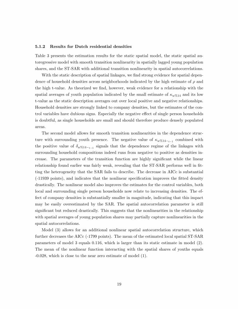
5.1.2 Results for Dutch residential densities

Table 3 presents the estimation results for the static spatial model, the static spatial au-

toregressive model with smooth transition nonlinearity in spatially lagged young population

shares, and the ST-SAR with additional transition nonlinearity in spatial autocorrelations.

With the static description of spatial linkages, we find strong evidence for spatial depen-

dence of household densities across neighborhoods indicated by the high estimate of ρ and

the high t-value. As theorized we find, however, weak evidence for a relationship with the

spatial averages of youth population indicated by the small estimate of κw%14 and its low

t-value as the static description averages out over local positive and negative relationships.

Household densities are strongly linked to company densities, but the estimates of the con-

trol variables have dubious signs. Especially the negative effect of single person households

is doubtful, as single households are small and should therefore produce densely populated

areas.

The second model allows for smooth transition nonlinearities in the dependence struc-

ture with surrounding youth presence. The negative value of κw%14−t−1combined with

the positive value of δw%14−t−1signals that the dependence regime of the linkages with

surrounding household compositions indeed runs from negative to positive as densities in-

crease. The parameters of the transition function are highly significant while the linear

relationship found earlier was fairly weak, revealing that the ST-SAR performs well in fit-

ting the heterogeneity that the SAR fails to describe. The decrease in AICc is substantial

(-11939 points), and indicates that the nonlinear specification improves the fitted density

drastically. The nonlinear model also improves the estimates for the control variables, both

local and surrounding single person households now relate to increasing densities. The ef-

fect of company densities is substantially smaller in magnitude, indicating that this impact

may be easily overestimated by the SAR. The spatial autocorrelation parameter is still

significant but reduced drastically. This suggests that the nonlinearities in the relationship

with spatial averages of young population shares may partially capture nonlinearities in the

spatial autocorrelations.

Model (3) allows for an additional nonlinear spatial autocorrelation structure, which

further decreases the AICc (-1799 points). The mean of the estimated local spatial ST-SAR

parameters of model 3 equals 0.116, which is larger than its static estimate in model (2).

The mean of the nonlinear function interacting with the spatial shares of youths equals

-0.028, which is close to the near zero estimate of model (1).

19

Table 3: Estimation results for Dutch residential densities from 2005-2014. Significance at90, 95 and 99% level are, respectively, indicated as *, ** and ***. t-values in parenthesis.Diebold-Mariano tests are one-sided against the previous model, and based on estimatesusing 2005-2013 data.

(1)SAR

+ WX

(2)SAR

+ ST-WX

(3)ST-SAR

+ ST-WX

βconst2.309***(26.531)

0.970***(36.611)

0.975***(41.894)

βcdenst−1

1.043***(201.134)

0.108***(21.805)

0.109***(28.381)

βwcdenst−1

-0.825***(-58.557)

-0.101***(-13.834)

-0.147***(-31.390)

β%1pshht−1

-0.006***(-9.320)

0.009***(34.365)

0.009***(38.670)

βw%1pshht−1

-0.025***(-17.745)

0.013***(23.710)

0.009***(19.946)

βw%hhkidst−1

-0.032***(-12.355)

0.018***(17.611)

0.015***(17.864)

β%nwimt−1

0.019***(35.607)

0.003***(12.348)

0.001***(3.170)

δw%14−t−1

1.008***(21.324)

0.541***(25.343)

γw%14−t−1

0.209***(22.501)

0.363***(34.370)

φw%14−t−1

1.742***(23.416)

0.275***(9.89)

κw%14−t−1

0.009*(1.987)

-0.432***(-27.409)

-0.387***(29.141)

δρ0.779***(69.597)

0.048***(7.113)

0.368***(35.28)

γρ1.235***(26.499)

φρ1.358***(84.993)

ν3.013***(23.933)

2.508***(25.772)

2.561***(26.745)

σ0.394***(30.184)

0.192***(27.07)

0.162***(17.358)

LL -2078.771 3893.733 4795.447AICc 4179.58 -7759.407 -9558.818DMFE 9.920*** 1.937**DMSFE 4.023*** 1.093

20

Figure 3: Left): spatial distribution of the time average of estimated autocorrelation pa-rameters. Right): spatial distribution of the time average of estimated dependence on theshare on population under 14 years in surrounding neighborhoods.

Figure 4: Left): Squared Forecast Errors of the SAR for one-step ahead predictions of the

change in the 2014 distribution. Right): Squared Forecast Errors of the ST-SAR based for

one-step ahead predictions of the change in the 2014 distribution. Legends are based on

natural breaks of the errors of the ST-SAR.

21

The maps in fig. 3 show that spatial autocorrelation is high in the urban clusters and

decays outwards. The linkages with surrounding youth population shares, move in a similar

direction along the urban gradient. Using estimates obtained using the data from 2005-2013,

we forecast the distribution of densities for 2014. Diebold-Mariano tests using the SFE for

the observations for 2014 are included in table 3 and show that the nonlinear specification

not only improves the fitted density but also significantly improves out-of-sample forecasts.

The maps in figure 4 compare the changes forecasted by the SAR and the ST-SAR+ST-

WX against the observed changes of 2014. The SFE for the static model clearly reveals

a consistent mismatch in major urban areas. The forecast errors of the nonlinear model,

however, seem to balance evenly across different areas. This shows that the nonlinear model

is better at fitting both rural and urban density processes within one framework. Apart from

the clustering of prediction errors, the predictive power across all regions is tremendously

improved by the nonlinear model.

5.2 Financial stability across the Euro region

In this second empirical study we evaluate the evolution of interest rates on government

bonds maturing in ten years for 15 European sovereigns over a period that includes the

formation of the European Union, its expansion, the Great Recession and the eventual

Greek sovereign debt crisis. Government bonds are essential to the functioning of financial

markets and government finances. On the supply side, governments issue debt securities

to support spending or finance deficits. On the demand side, institutions and investors use

them to manage overall portfolio risk and may require them as part of funding operations.

The yields on sovereign debts also play a central role in the pricing and risk-assessment of

other financial instruments or investments, because they represent available minimal-risk

rates. The yield curves on sovereign debt reflect the overall trust of investors in the stability

of economies and provide a policy indicator used by governments to guard the state of their

economy.

The Economic and Monetary Union (EMU) comprises a set of policies that aims at con-

verging the economies of the member states of the European Union. The EMU prescribes

the euro convergence criteria, comprising the prerequisites for a nation to join the eurozone.

Co-movement in the long term interest rates is essential to the monetary stability of the

Euro region. Before the European Union, the European Economic Community relied heav-

ily on the European Exchange Rate Mechanism (ERM) to regulate variability in exchange

rates of different sovereigns as a way to achieve monetary stability. The ERM played a

central role in the preparations for the Economic and Monetary Union and the subsequent

introduction of the euro in 1999. The primary goal of the ERM has been to prevent large

fluctuations in currency values relative to those of other European sovereigns. Adjustments

22

in national interest rates have been at the center of monetary policy used as part of the

European Monetary System (EMS) to lower or increase currency value such that the differ-

ent currencies remained within a narrow range of one another. Replacement of the actual

currencies of all participating member states by a common currency mandates that the

economies of all member states are relatively in par with one another. After introduction

of the euro, national interest rates still play an essential role in ensuring that fluctuation in

the economies of all member states remains within a narrow range.

A strong adjustment in long term interest rate of a particular sovereign with respect

to the common European average, signals that the underlying economy has difficulty in

following the common trend. On the other hand, if all interest rates closely share a common

stochastic trend, it signals that economies are in par with on another. The ST-SAR provides

a direct method to analyze the strength of convergence toward a common stochastic trend.

The average cross-sectional dependence signals the average strength of convergence toward

the common, whereas a low average dependence signals that countries are weakly attracted

to the common trend. Additionally, low dependence of an individual sovereign signals a

potential decoupling of that economy from the common stochastic trend, which may for

example result from sustained policy interventions or other local exogenous shocks. The

cross-sectional standard deviations in the contraction parameters provides an indicator of

the overall financial stability in the Euro region, a high standard deviation indicates that

there is substantial difference in the strength of the convergence rates of individual member

countries toward the common trend, and a low standard deviation in combination with

positive average cross-sectional contraction indicates that the commonality dominates across

all individual members. The parameters of the ST-SAR are therefore provide one way to

inform us on the functioning of the EMS.

5.3 European Long term Interest Rates

We view the interest rates as generated by the model:

Vt = ct + Yt,

where Vt is the observed data vector, ct is the common stochastic trend, and Yt is a vector

of dynamics around the common stochastic trend. We are interested it analyzing Yt, which

contains the contraction and dispersion dynamics around the common stochastics. We

assume ct to follow a random walk with ct = ct−1 +vt, and vtt∈Z ∼ pv(vt,Σ, λ). Therefore

23

our best expectation of ct is ct ∼ EN (Yt|Yt−1), and the dynamics of particular interest are:

Yt = Vt − EN (Vt|Vt−1) = Vt − EN (Vt−1) ∼ Vt −N−1N∑1

(Vt−1),

hence we use Yt = Vt − N−1∑N

1 (Vt−1) as our dependent variable. We refer to Yt as

the detrended data. We are interested in a description of the convergence and dispersion

dynamics contained in Yt as a nonlinear cross-sectional dependence process driven by the

past states of Yt and moving average affects. As a first exploration we regress models of the

type:8

Yt = H(θρ; (Yt−p, εt−p))−1(εt).

In our extended results, we allow for additional flexibility and explore

Yt = H(θρ; (Yt−p, εt−p))−1g(θg;Yt−p, εt−p, εt),

to distinguish between effects that move through the cross-sectional dependence structure

or directly though an ARMA structure modeled by g(θg;Yt−p, εt−p, εt) with ε1:p initialized

at zero. We explore lags up to order 4, and apply zero restrictions guided by the AICc.

As we shall see in our final model, allowing for lags up to order 4 is sufficient to render

the residuals free of significant correlations, with some of the parameters restricted to zero.

We contrast the models with a linear SAR counterpart. Our spatial structure is based on

thresholding of the correlation matrix extracted from the detrended data. This allows for

a differential in the centrality of the different sovereigns in the economic network and for

entanglement between sovereigns that are distant from each other in a geographic sense but

share strong co-movements. We allow each cross-sectional unit to have three neighbors in

the network. This number was picked by comparing the AICc of the SAR for networks with

respectively 2, 3 and 4 neighbors.

5.3.1 Long term interest rates data

We use relative changes (log returns multiplied by 100) of long term interest rates obtained

from the OECD, and include observations for 278 months starting October 1993.9 The de-

trended log returns are visualized in fig. 5, the raw data including a list of labelled events and

color codes is provided in Appendix A.3.1. The time series reveal clear common patterns,

especially between 1998 and 2008. Before 1998 and after 2008 there are commonalities but

8The exact threshold specified as ρ(θρ;Yt, εt) =δ

1 + exp(−γ(WYt−1 − (α+ Yt−pϕφ + εt−pϕµ)))+ κ.

9https://data.oecd.org/interest/long-term-interest-rates

24

Table 4: ADF tests without constant on demeaned sequences. Lags are equal across tests toallow a comparison, and determined by estimating AR(AICc) on the cross-sectional mean.Critical values are not adjusted with a Bonferroni correction.

Sovereign ADF Stable

Austria -2.227 stationaryBelgium -2.945 stationaryGermany -1.382 nonstationaryDenmark -1.708 stationarySpain -1.517 nonstationaryFinland -1.737 stationaryFrance -2.976 stationaryUnited Kingdom -1.991 stationaryGreece -0.805 nonstationaryIreland -1.829 stationaryItaly -1.318 nonstationaryNetherlands -1.970 stationarySweden -1.887 stationaryPortugal 0.241 nonstationaryLuxembourg -1.692 stationary

Cross-sectional mean -7.815 stationary

specifically the stressed Eurozone sovereigns (Greece, Portugal, Ireland and to some extent

Spain and Italy), seem to follow a separate pattern. Table 4 highlights this erratic behavior,

and shows that individually, these sovereigns - in addition to Germany that was first to ever

hit a negative rate - follow nonstationary trajectories.

5.3.2 Results using European long term interest rates

Table 5 contains the estimation results from both the static and nonlinear spatial model

for different specifications of the threshold process. The data exhibits very heavy tails,

and for simplicity we have fixed λ at 2.5 in all models. In the static model, we find strong

evidence for spatial dependence in the returns of the rates indicated by the high estimate for

ρ together with a small standard error. The three nonlinear specifications, respectively the

ST-SAR driven by past observations, moving averages and combinations thereof, all improve

the AICc values by several thousand points compared to the SAR, providing ample evidence

for nonlinearities in the convergence and dispersion process. The results suggest that the

spatial dynamics are driven both by past observations as well as moving averages. On the

basis of the reported AICc values, the data clearly favors dynamical spatial dependence.

25

1.2

1.4

1.6

1.8

2.0

Detrended Monthly Long−term Interest Rates for 15 EU countries

date

Rat

es

10−1993 04−1996 10−1998 04−2001 10−2003 04−2006 10−2008 04−2011 10−2013 04−2016

12

3 45, 6 7, 8 9

12

1516

1718 19 20

21

22 23 24

Cross−sectional averageCross−sectional QuartilesMajor European events

0.0

0.2

0.4

0.6

0.8

Standard diviations of the cross−section interest rates

date

Sta

ndar

d de

viat

ions

10−1993 04−1996 10−1998 04−2001 10−2003 04−2006 10−2008 04−2011 10−2013 04−2016

Pre−EU Early−EU Financial crisis Great Recession

Greek souvereign debt crisis

01

23

4

Monthly log Long−term Interest Rates

Contraction and expansion as set by The Centre for Economic Policy Research

log(

1+re

turn

s)

10−1993 04−1996 10−1998 04−2001 10−2003 04−2006 10−2008 04−2011 10−2013 04−2016

ContractionExpansion

Figure 5: Data on monthly long term interest rates for bonds of 10-year maturity. Anoverview of te labelled events is contained in Appendix A.3.1.

26

However, the SAR contains no time dynamics, which allows the possibility that the nonlinear

models attempt to fit time autoregressive forces through the spatial dependence parameters.

We therefore extend our analysis by modeling additional dynamics in the time dimension.

5.3.3 Extensions

Table 6 presents the estimation results for the models with ARMA effects running through

the main time-series process. Again, we observe that the nonlinear spatial model improves

the AICc substantially, approximately by -2406 points. The improvement is confirmed by

Diebold-Mariano tests on the one-step ahead forecasts, with a DM = 20.01 for residuals,

and DM = 7.37 for squared residuals. The results provide evidence that the ST-SAR

nonlinearities are robust to the specification of different time dynamics, and explain an

important part of the variation within the data.

Figure 6 displays the evolution of the fitted spatial dependence parameters. Across the

entire time-span, average contraction remained high. A striking feature is the convergence

of the spatial parameters in anticipation of the Union, continuing till around 2000. In the

pre-EU period we observe two separate regimes. Ireland, Portugal, Italy and Spain form a

group that has lower attraction to the common trend, while the remaining sovereigns form

a group with a stronger attraction to the common. Greece seems to form an exception and

follows an individual trajectory.

After 2000, the parameter sequences corresponding to the different sovereigns nearly

linearize. The standard deviations in the parameters remain close to zero for a prolonged

period, indicating strong financial stability and near perfect co-movement in the evolution

of the individual rates. The onset of the Great Recession around 2008 marks an abrupt

turn after which separation in a high and low regime recurs. The standard deviation in

attraction parameters attains a peak during the 2012 crisis as rates of stressed sovereigns

surge while the remaining nations continue on a downward trend. The months after 2014 are

marked by further dispersion. Just before 2015, as Germany hits negative rates for the first

time recorded, the range in parameters peaks. Interestingly, the pattern after the recession

seems to revert to the pre-EU behavior, with Greece returning to an individual trajectory

and Ireland, Portugal, Italy and Spain forming a group of sovereigns that are less bound to

the common evolution path. Divergence between the low and high dependence regimes has

continued, and the sustained strong variation in contraction parameters indicates that the

Eurozone remains to struggle in attaining financial stability since the onset of the financial

crisis. The decline in attraction to the common trend for Ireland, Portugal, Italy, and Spain

is in sharp contrast to the increase across other member states, and suggests that the EMS

has not fully succeeded in aligning these economies of with the rest of the Eurozone, while

27

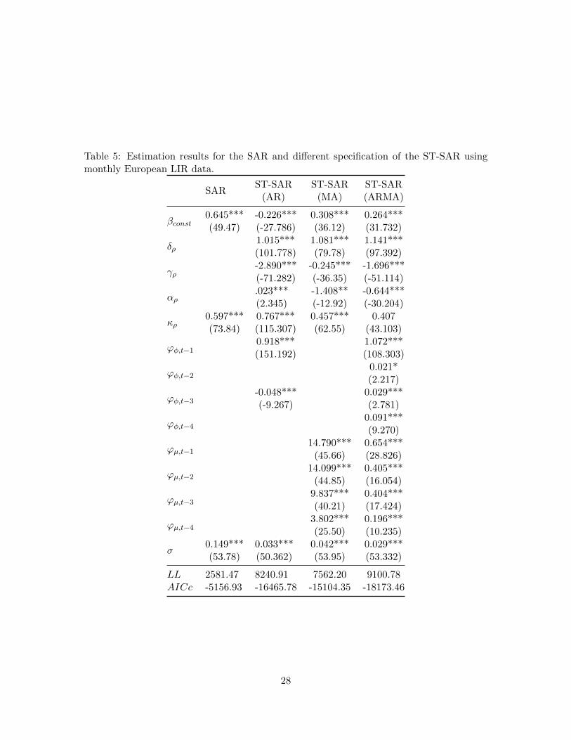
Table 5: Estimation results for the SAR and different specification of the ST-SAR usingmonthly European LIR data.

SARST-SAR

(AR)ST-SAR

(MA)ST-SAR(ARMA)

βconst0.645***(49.47)

-0.226***(-27.786)

0.308***(36.12)

0.264***(31.732)

δρ1.015***(101.778)

1.081***(79.78)

1.141***(97.392)

γρ-2.890***(-71.282)

-0.245***(-36.35)

-1.696***(-51.114)

αρ.023***(2.345)

-1.408**(-12.92)

-0.644***(-30.204)

κρ0.597***(73.84)

0.767***(115.307)

0.457***(62.55)

0.407(43.103)

ϕφ,t−10.918***(151.192)

1.072***(108.303)

ϕφ,t−20.021*(2.217)

ϕφ,t−3-0.048***(-9.267)

0.029***(2.781)

ϕφ,t−40.091***(9.270)

ϕµ,t−114.790***

(45.66)0.654***(28.826)

ϕµ,t−214.099***

(44.85)0.405***(16.054)

ϕµ,t−39.837***(40.21)

0.404***(17.424)

ϕµ,t−43.802***(25.50)

0.196***(10.235)

σ0.149***(53.78)

0.033***(50.362)

0.042***(53.95)

0.029***(53.332)

LL 2581.47 8240.91 7562.20 9100.78AICc -5156.93 -16465.78 -15104.35 -18173.46

28

attraction between other sovereigns is currently at an all time high.0.

50.

60.

70.

80.

91.

0

Estimated cross−sectional dependence parameters for 15 EU countries

date

Cro

ss−

sect

iona

l dep

ende

nce

08−1993 02−1996 08−1998 02−2001 08−2003 02−2006 08−2008 02−2011 08−2013 02−2016

1 2

3 4 5, 67, 8

9 12 15161718 19 20 21 22 23

24

Cross−sectional averageCross−sectional QuartilesMajor European events

−0.

10.

00.

10.

20.

30.

4

Cross−section standard diviations of the dependence parameters

date

Sta

ndar

d de

viat

ions

08−1993 02−1996 08−1998 02−2001 08−2003 02−2006 08−2008 02−2011 08−2013 02−2016

Pre−EU Early−EU Financial crisis Great Recession

Greek souvereign debt crisis

0.5

0.6

0.7

0.8

0.9

1.0

1.1

1.2

Estimated cross−sectional dependence parameters for 15 EU countries

Contraction and expansion as set by The Centre for Economic Policy Research

Cro

ss−

sect

iona

l dep

ende

nce

08−1993 02−1996 08−1998 02−2001 08−2003 02−2006 08−2008 02−2011 08−2013 02−2016

ContractionExpansion

Figure 6: Evolution of spatial parameters estimated with the ST-SAR.

A final noteworthy result is that the residuals of the nonlinear model, as in application

our first application, are better centered at zero. Specifically the SAR residuals correspond-

ing to Spain and Greece remain respectively below and above zero for prolonged periods.

This can be seen in fig. 10. The residuals of the SAR specification contain significant remain-

ing correlation patterns while the ST-SAR neutralize the dynamics using one autoregressive

parameter less in the main equation. This is revealed by the ACF and PACF plotted in

fig. 11. Both figures are contained in Appendix A.3.1.

29

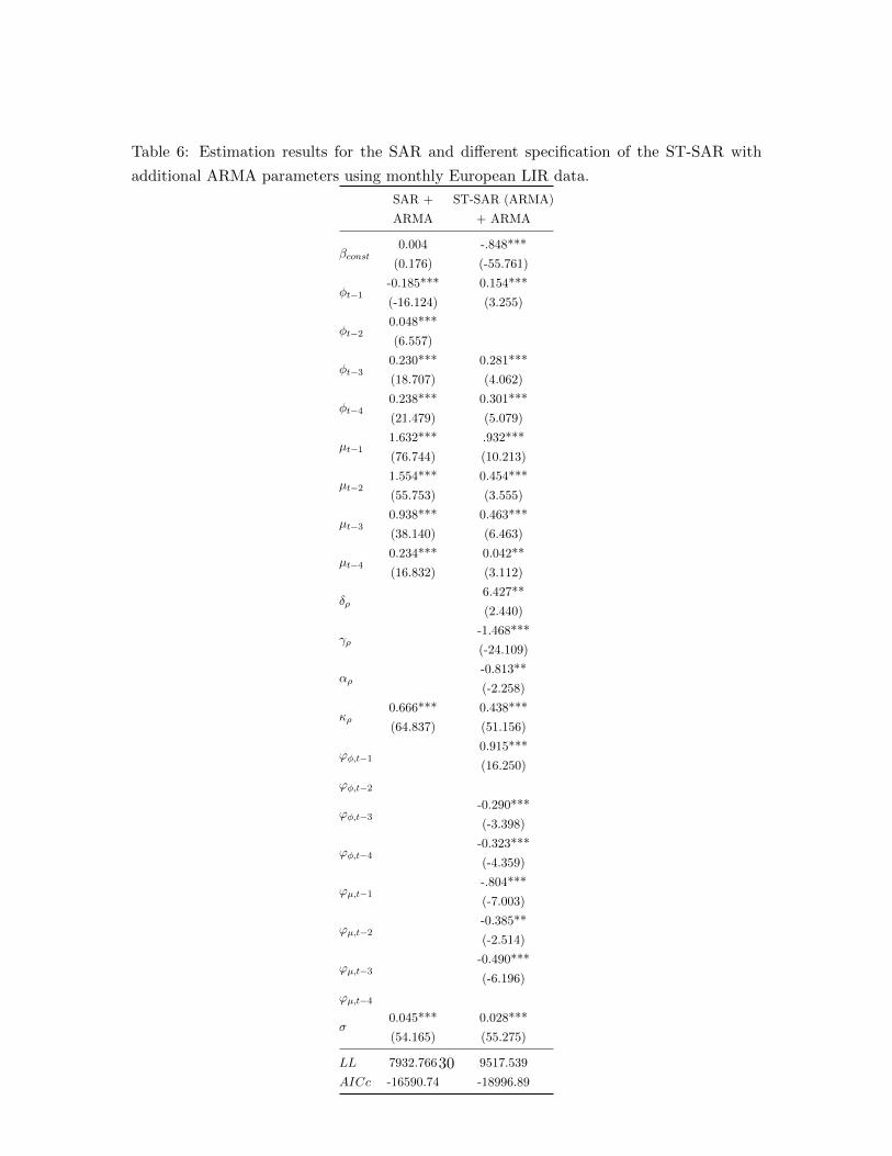
Table 6: Estimation results for the SAR and different specification of the ST-SAR with

additional ARMA parameters using monthly European LIR data.

SAR +

ARMA

ST-SAR (ARMA)

+ ARMA

βconst0.004

(0.176)

-.848***

(-55.761)

φt−1-0.185***

(-16.124)

0.154***

(3.255)

φt−20.048***

(6.557)

φt−30.230***

(18.707)

0.281***

(4.062)

φt−40.238***

(21.479)

0.301***

(5.079)

µt−11.632***

(76.744)

.932***

(10.213)

µt−21.554***

(55.753)

0.454***

(3.555)

µt−30.938***

(38.140)

0.463***

(6.463)

µt−40.234***

(16.832)

0.042**

(3.112)

δρ6.427**

(2.440)

γρ-1.468***

(-24.109)

αρ-0.813**

(-2.258)

κρ0.666***

(64.837)

0.438***

(51.156)

ϕφ,t−10.915***

(16.250)

ϕφ,t−2

ϕφ,t−3-0.290***

(-3.398)

ϕφ,t−4-0.323***

(-4.359)

ϕµ,t−1-.804***

(-7.003)

ϕµ,t−2-0.385**

(-2.514)

ϕµ,t−3-0.490***

(-6.196)

ϕµ,t−4

σ0.045***

(54.165)

0.028***

(55.275)

LL 7932.766 9517.539

AICc -16590.74 -18996.89

30

6 Conclusion

In this paper we introduced a new model for nonlinear spatial time series in which cross-

sectional dependence varies smoothly over space by means of a specification that allows

for smooth-transitions between multiple dependence regimes. In this framework, nonlin-

earities in cross-sectional dynamics are directly modeled as a function of the data. This is

an advance over existing methods that rely on ad-hoc sample divisions, ambiguous dummy

specifications, or weighted parameter vectors derived from geographic kernel density es-

timates. All whom are known to have serious drawbacks. Allowing for time-variation is

particularly useful when modeling spatial contraction over long time periods - it cannot

be assumed that spatial dependence remains fixed for prolonged periods. In addition, the

nonlinearities over the cross-section are particularly useful if N is large - as in our first

application - or when dispersion and convergence dynamics are key features of the data -

as in our second application.

We have shown that the parameters of the model can be consistently estimated by

maximum likelihood under appropriate regularity conditions. In particular, we provide

conditions that deliver existence, strong consistency and asymptotic normality of the MLE

of all static parameters that constitute the dynamic dependence structure. The theory holds

for both correctly specified and misspecified models. Additional results made available

in a Supplementary Appendix deliver the geometric ergodicity of data generated by the

ST-SAR model. Our simulation evidence suggests that the limit theory is relevant and

that the ML estimator behaves well in finite samples. Furthermore, we find that standard

information criteria are able to distinguish between the SAR specification and ST-SAR type

nonlinearities. The simulations results showed that model selection is robust to overfitting

of additive outliers.

Our empirical applications on Dutch household densities and European long term in-

terest rates, provide ample evidence that spatial nonlinearities are not only persistent, but

also explain a major part of the observed dynamics. Across our applications we find that

ST-SAR improves in- and out-of-sample forecasts, reduces AICc, and better neutralizes

residual correlation. We find that spatial dependence in is driven both exogenously and

endogenously, and reacts to the slow assimilation of exogenous shocks.

31

7 References

References

Akaike, H. (1973). Information theory and an extension of the maximum likelihood principle.

Technical report.

Akaike, H. (1974). A new look at the statistical model identification. IEEE Transactions

on Automatic Control, 19(6):716–723.

Anselin, L. (1988). Spatial Econometrics: Methods and Models.

Anselin, L. (1995). Local Indicators of Spatial Association-LISA. Geographical Analysis,

27(2):93–115.

Baltagi, B. H., Fingleton, B., and Pirotte, A. (2014). Spatial lag models with nested random

effects: An instrumental variable procedure with an application to English house prices.

Journal of Urban Economics, 80:76–86.

Bao, Y. and Ullah, A. (2007). Finite sample properties of maximum likelihood estimator

in spatial models. Journal of Econometrics, 137(2):396–413.

Basile, R., Durban, M., Mınguez, R., Marıa Montero, J., and Mur, J. (2014). Modeling re-

gional economic dynamics: Spatial dependence, spatial heterogeneity and nonlinearities.

Journal of Economic Dynamics and Control, 48:229–245.

Baumont, C., Ertur, C., and Gallo, J. L. (2006). The European Regional Convergence

Process, 1980-1995: Do Spatial Regimes and Spatial Dependence Matter? International

Regional Science Review, 29(1):1–41.

Billingsley, P. (1961). The Lindeberg-Levy Theorem for Martingales. Proceedings of the

American Mathematical Society, 12(5):788.

Blasques, F., Koopman, S. J., Lucas, A., and Schaumburg, J. (2016). Spillover dynamics

for systemic risk measurement using spatial financial time series models. Journal of

Econometrics, 195(2):211–223.

Bonhomme, S. and Manresa, E. (2015). Grouped Patterns of Heterogeneity in Panel Data.

Econometrica, 83(3):1147–1184.

Brockwell, P. J. and Davis, R. A. (1991). Time Series: Theory and Methods. Springer.

Burnham, K. P. and Anderson, D. R. (2004). Multimodel inference: understanding aic and

bic in model selection. Sociological Methods & Research, 33:261–304.

32

Cho, S.-H., Lambert, D. M., and Chen, Z. (2010). Geographically weighted regression

bandwidth selection and spatial autocorrelation: an empirical example using Chinese

agriculture data. Applied Economics Letters, 17(8):767–772.

Cliff, A. and Ord, J. (1969). The Problem of Spatial Autocorrelation. In A. J. Scott, editor,

In London Papers in Regional Science, pages 25–55. Pion, London.

Cline, D. B. H. and Pu, H.-M. H. (1998). Verifying irreducibility and continuity of a

nonlinear time series. Statistics & Probability Letters, 40:139–148.

Cline, D. B. H. and Pu, H.-M. H. (1999). Geometric Ergodicity of Nonlinear Time Series.

Statistica Sinica, 9:1103–1118.

Comte, F. and Lieberman, O. (2003). Asymptotic theory for multivariate GARCH processes.

Journal of Multivariate Analysis, 84(1):61–84.

Crase, B., Liedloff, A. C., and Wintle, B. A. (2012). A new method for dealing with residual

spatial autocorrelation in species distribution models. Ecography, 35(10):879–888.

Das, D., Kelejian, H. H., and Prucha, I. R. (2003). Finite sample properties of estimators

of spatial autoregressive models with autoregressive disturbances. Papers in Regional

Science, 82(1):1–26.

Debarsy, N., Jin, F., and Lee, L.-f. (2015). Large sample properties of the matrix exponential

spatial specification with an application to FDI. Journal of Econometrics, 188(1):1–21.

Dijk, D., Terasvirta, T., and Franses, P. (2002). Smooth transition autoregressive models—a

survey of recent developments. Econometric Reviews, (August 2013):37–41.

Dijk, D. V., Franses, P. H., Lucas, A., and Lucas, A. (1999). Testing for Smooth Transition

Nonlinearity in the Presence of Outliers. Journal of Business & Economic Statistics,

17(2):217.

Dudley, R. M. (2002). Real Analysis and Probability. Cambridge Studies in Advanced

Mathematics. Cambridge University Press.

Epple, D. and Sieg, H. (1999). Estimating Equilibrium Models of Local Jurisdictions. The

Journal of Political Economy, 10(2):130–153.

Farber, S. and Paez, A. (2007). A systematic investigation of cross-validation in GWR model

estimation: Empirical analysis and Monte Carlo simulations. Journal of Geographical

Systems, 9(4):371–396.

33

Foland, G. B. (2009). A Guide to Advanced Real Analysis. Dolciani Mathematical Exposi-

tions. Cambridge University Press.

Fotheringham, A. S. (1981). Spatial structure and distance-decay parameters. Annals of

the Association of American Geographers, 71(3):425–436.

Fotheringham, A. S. (2009). “The Problem of Spatial Autocorrelation” and Local Spatial

Statistics. Geographical Analysis, 41(4):398–403.

Fotheringham, A. S., Brunsdon, C., and Charlton, M. (2002). Geographically Weighted

Regression: The Analysis of Spatially Varying Relationships.

Frıas, M. and Ruiz-Medina, M. (2016). Wavelet nonparametric estimation from strong

spatial correlated high-dimensional data. Spatial Statistics, 18:363–385.

Gallant, R. and White, H. (1988). A Unified Theory of Estimation and Inference for

Nonlinear Dynamic Models. Cambridge University Press.

Glass, A. J., Kenjegalieva, K., and Sickles, R. C. (2016). A spatial autoregressive stochastic

frontier model for panel data with asymmetric efficiency spillovers. Journal of Economet-

rics, 190(2):289–300.

Granger, C. W., King, M. L., and White, H. (1995). Comments on testing economic theories

and the use of model selection criteria. Journal of Econometrics, 67(1):173–187.

Granger, W. J. and Terasvirta, T. (1993). Modelling Nonlinear Economic Relationships.

Oxford University Press, 61(4):1241–1243.

Hoshino, T. (2016). Semiparametric Spatial Autoregressive Models with Endogenous Re-

gressors: With an Application to Crime Data. Journal of Business & Economic Statistics,

pages 1–51.

Hurvich, C. and Tsai, C.-L. (1989). Regression and time series model selection in small

samples. Biometrika, 76:297–307.

Kelejian, H. H. and Prucha, I. R. (2010). Specification and estimation of spatial autore-

gressive models with autoregressive and heteroskedastic disturbances. Journal of Econo-

metrics, 157(1):53–67.

Kostov, P. (2009). A Spatial Quantile Regression Hedonic Model of Agricultural Land

Prices. Spatial Economic Analysis, 4(1):53–72.

Krengel, U. (1985). Ergodic theorems. Walter de Gruyter.

34

Kullback, S. and Leibler, R. A. (1951). On Information and Sufficiency. The Annals of

Mathematical Statistics, 22(1):79–86.

Lange, K. (1999). Numerical analysis for statisticians. Springer.

Lee, L. F. (2004). Asymptotic distributions of quasi-maximum likelihood estimators for

spatial autoregressive models.

LeSage, J. P. (2008). An Introduction to Spatial Econometrics. Revue d’economie indus-

trielle, 123(123):19–44.

LeSage, J. P. and Fischer, M. M. (2008). Spatial growth regressions: Model specification,

estimation and interpretation. Spatial Economic Analysis, 3(3):275–304.

Leung, Y., Mei, C. L., and Zhang, W. X. (2000a). Statistical tests for spatial nonstationarity

based on the geographically weighted regression model. Environment and Planning A,

32(1):9–32.

Leung, Y., Mei, C. L., and Zhang, W. X. (2000b). Testing for spatial autocorrelation among

the residuals of the geographically weighted regression. Environment and Planning A,

32(5):871–890.

McQuarrie, A. D. R.; Tsai, C.-L. (1998). Regression and time series model selection. World

Scientific.

Ord, K. (1975). Estimation Methods for Models of Spatial Interaction. Journal of the

American Statistical Association, 70(349):120–126.

Paez, A., Uchida, T., and Miyamoto, K. (2002a). A general framework for estimation and

inference of geographically weighted regression models: 1. Location-specific kernel band-

widths and a test for locational heterogeneity. Environment and Planning A, 34(4):733–

754.

Paez, A., Uchida, T., and Miyamoto, K. (2002b). A general framework for estimation and

inference of geographically weighted regression models: 2. Spatial association and model

specification tests. Environment and Planning A, 34(5):883–904.

Potscher, B. M. and Prucha, I. R. (1997). Dynamic Nonlinear Econometric Models. Springer

Berlin Heidelberg, Berlin, Heidelberg.

Rao, R. R. (1962). Relations between Weak and Uniform Convergence of Measures with

Applications. The Annals of Mathematical Statistics, 33(2):659–680.

35

Sin, C.-Y. and White, H. (1996). Information criteria for selecting possibly misspecified

parametric models. Journal of Econometrics, 71(1):207–225.

Straumann, D. and Mikosch, T. (2006). Quasi-maximum-likelihood estimation in condi-

tionally heteroeskedastic time series: A stochastic recurrence equations approach. The

Annals of Statistics, 34(5):2449–2495.

Su, S., Xiao, R., and Zhang, Y. (2012). Multi-scale analysis of spatially varying relationships

between agricultural landscape patterns and urbanization using geographically weighted

regression. Applied Geography, 32(2):360–375.

Terasvirta, T. (1994). Specification, Estimation and Evaluation of Smooth Transition Au-

toregressive Models. Journal of the American Statistical Association, 89(425):208–218.

Terasvirta, T. and Anderson, H. M. (1992). Terasvirta Anderson 1992 Characterizing Non-

linearities in Business Cycles Using Smooth Transition Autoregressive Models. Journal

of Applied Econometrics, 7(S):S119–36.

Tong, H. (1978). On a Threshold Model. In Pattern Recognition and Signal Processing,

number January 1978, pages 575–586.

Tong, H. (2015). Threshold models in time series analysis—Some reflections. Journal of

Econometrics, 189(2):485–491.

Tsay, R. S. (1989). Testing and Modeling Threshold Autoregressive Processes. Journal of

the American Statistical Association, 84(405):231–240.

van der Vaart, A. W. (2000). Asymptotic Statistics (Cambridge Series in Statistical and

Probabilistic Mathematics). Cambridge University Press.

Wheeler, D. and Tiefelsdorf, M. (2005). Multicollinearity and correlation among local

regression coefficients in geographically weighted regression. Journal of Geographical

Systems, 7(2):161–187.

Wheeler, D. C. (2007). Diagnostic tools and a remedial method for collinearity in geograph-

ically weighted regression. Environment and Planning A, 39(10):2464–2481.

White, H. (1994a). Estimation, inference, and specification analysis. Cambridge University

Press.

White, H. (1994b). Estimation, Inference and Specification Analysis. Cambridge Books.

Cambridge University Press.

36

A Apendix

A.1 Proof of Theorem 1

Proof. Note first that `T (θ) := (1/T )∑T

t=1 `t(θ) is a.s. continuous (a.s.c.) in θ ∈ Θ through

continuity (c.) of each term `t(θ) = ln detH(θρ;Zt) + ln pε(H(θρ;Zt)Yt − φYt−1 − Xtβ −µεt−1,Σ;λ). Together with the compactness of Θ (Assumption 1) this implies by Weier-

strass’ theorem that the arg max set is non-empty a.s. and hence that θT exists a.s. ∀T ∈ N.

Note by a similar argument that `T (θ) is continuous in (Yt, Xt) ∀ θ ∈ Θ and hence measur-

able w.r.t. the product Borel σ-algebra B(Y) ⊗B(X ) that are, in turn, measurable maps

w.r.t. F by Proposition 4.1.7 in Dudley (2002).10 Finally, the measurability of θT follows

from (Foland, 2009, p.24) and (White, 1994b, Theorem 2.11) or (Gallant and White, 1988,

Lemma 2.1, Theorem 2.2).11


Proof. Following a classical consistency argument (found e.g. in (White, 1994b, Theorem

3.4) or Theorem 3.3 in Gallant and White (1988)) we obtain θTa.s.→ θ0 from the uniform

convergence of the criterion function

supθ∈Θ|`T (θ)− `∞(θ)| a.s.→ 0 ∀ f1 ∈ F as T →∞ (12)

and the identifiable uniqueness of the maximizer θ0 ∈ Θ introduced in White (1994b),

supθ:‖θ−θ0‖>ε

`∞(θ) < `∞(θ0) ∀ ε > 0. (13)

The uniform convergence is obtained by norm sub-additivity,12

supθ∈Θ|`T (θ)− `∞(θ)| ≤ sup

θ∈Θ|`T (θ)− `T (θ)|+ sup

θ∈Θ|`T (θ)− `∞(θ)|

and then for the first term showing that

supθ∈Θ|`T (θ)− `T (θ)| a.s.→ 0 as T →∞ (14)

10Dudley’s proposition states that the Borel σ-algebra B(A × B) generated by the Tychonoff’s producttopology TA×B on the space A× B includes the product σ-algebra B(A)⊗ B(B).

11The reference of Foland (2009) is used here to establish that a map into a product space is measurableif and only if its projections are measurable.

12`T (θ) denotes the limit as T → ∞ of `T (θ) defined as `T (θ) := (1/T )∑Tt=1 `t(θ) with `t(θ) defined in

(9).

37

and for the second term applying the ergodic theorem for separable Banach spaces in Rao

(1962), as in (Straumann and Mikosch, 2006, Theorem 2.7), to the sequence `T (·) with

elements taking values in C(Θ,R) so that supθ∈Θ |`T (θ)−`∞(θ)| where `∞(θ) = E`t(θ) ∀ θ ∈Θ.

The ULLN supθ∈Θ |`T (θ) − E`t(θ)|a.s.→ 0 as T → ∞ follows, under a moment bound

E supθ∈Θ |`t(θ)| < ∞, by the SE nature of `T t∈Z which is implied by continuity of ` on

the SE sequence (Yt, Xt)t∈Z (Assumption 2) and Proposition 4.3 in Krengel (1985). The

moment bound E supθ∈Θ |`t(θ)| <∞ follows immediately from Assumption 3 since

E supθ∈Θ|`t(θ)| ≤ E sup

θ∈Θ|Q(θρ;Zt)|+ |A(θ)|+ 1

2(λ+ n)E sup

θ∈Θ|F (θ, Yt, Xt, Zt)| <∞

Finally, the identifiable uniqueness (see e.g. White (1994b)) of θ0 ∈ Θ in (13) follows

from the assumed uniqueness (Assumption 3), the compactness of Θ, and the continuity of

the limit E`t(θ) in θ ∈ Θ which is implied by the continuity of `T in θ ∈ Θ ∀ T ∈ N and the

uniform convergence in (12).


Proof. We obtain the asymptotic Gaussianity of the MLE from (i) the strong consistency

of θTa.s.→ θ0 ∈ int(Θ); (ii) the a.s. twice continuous differentiability of `T (θ) in θ ∈ Θ; (iii)

the asymptotic normality of the score

√T`′T

(θ0)

d→ N(0,J (θ0)), J (θ0) = E

(`′t(θ0)`′t

(θ0)ᵀ

); (15)

(iv) the uniform convergence of the likelihood’s second derivative,

supθ∈Θ

∥∥`′′T (θ)− `′′∞(θ)∥∥ a.s.→ 0; (16)

and finally, (v) the non-singularity of the limit `′′∞(θ) = E`′′t (θ) = I(θ). See e.g. in (White,

1994b, Theorem 6.2)) for further details.

The consistency condition θTa.s.→ θ0 ∈ int(Θ) in (i) follows by Theorem 2 and the

additional assumption that θ0 ∈ int(Θ).

The smoothness condition in (ii) is trivially satisfied for the student’s-t density.

The asymptotic normality of the score in (17) follows by Theorem 18.10[iv] in van der

Vaart (2000) by an application of the CLT for SE martingales in Billingsley (1961) to obtain

√T`′T

(θ0)

d→ N(0,J (θ0))

as T →∞, (17)

38

where J (θ0) = E(`′t(θ0)`′t

(θ0)ᵀ) < ∞. The SE nature of `′T

(θ0)t∈Z follows by continuity

of `′ on the SE sequence (Yt, Xt)t∈Z; see Proposition 4.3 in Krengel (1985). Assumption

5 imposes the mds nature of `′T(θ0)t∈Z. The finite (co)variances follow from the first two

moments bounds of Assumption 6.

The uniform convergence in (iv)is obtained under the moment bound E supθ∈Θ ‖`′′t (θ)‖ <∞ and by the SE nature of `′′T t∈Z. The moment bound is ensured by Assumption 6. The

SE nature is implied by continuity of `′′ on the SE sequence Yt, Xtt∈Z.

Finally, the non-singularity of the limit `′′∞(θ) = E`′′t (θ) = I(θ) in (v) is implied by the

uniqueness of θ0 as a maximum of `′′∞(θ) in Θ.

39

Supplementary Appendix

Smooth Transition Spatial Autoregressive Models for

Cross-sectional Time Series

Bo Pieter Johannes Andree, Francisco Blasques, Eric Koomen

Additional Results

As a potential DGP the ST-SAR is capable of producing random data with interesting

nonlinear dynamics over time and space. Because of the multivariate nature of the model, a

proof for strict stationarity and ergodicity based on Lipschitz properties is unavailable, see

for example Comte and Lieberman (2003) for a discussion in the context of the multivartiate

GARCH.13. Therefore, results regarding strict stationarity and ergodicity of time-varying

spatial parameter models provided by Blasques et al. (2016) do not hold for the ST-SAR.

While the ST-SAR dynamics may be complex, under appropriate regularity conditions,

the model can still be shown to generate data that is geometrically ergodic. We focus on the

endogenous case where Zt = Yt and β = 0 as this is naturally the most interesting case for a

study on stability. Let θ denote the vector of parameters of our ST-SAR θ := (δ, γ, α, ϕ, κ, φ)′

and θ0 denote the vector of the true parameters of the endogenous ST-SAR. Under correct

specification, there exists θ0 ∈ Θ, such that an observed T−period data sequence Yt(ω)Tt=1

is a subset of a realized path of the n-variate stochastic sequence Y (ω) := Yt(ω)t∈Z, for

some event ω in the event space Ω with Yt(ω) ∈ Y ⊂ Rn ∀ (ω, t) ∈ Ω × Z living on the

space (Y∞,B(Y∞), P y0 ). P y0 here denotes the true probability measure, such that we are

concerned with a sequence Y (ω) generated by the model. Below we let ‖ · ‖∞ denote the

sup norm on Rn and ‖ · ‖ denote any matrix norm. For readability, we first present the

results and let the proofs follow at the end of the section.

Lemma 1. Let A be an arbitrary finite-dimensional matrix. For an induced matrix norm

‖A‖ < 1 the following inequality is implied:

(1 + ‖A‖)−1 ≤ ‖(In −A)−1‖ ≤ (1− ‖A‖)−1,

13A model Yt = F (Yt−1, εt) is Lipschitz if ‖F (x, ε)−F (y, ε)‖ ≤ α(ε)‖x− y‖ for a positive valued functionα with E(α(εt)

m) < 1 and E(‖F (0, |εt)‖m) <∞ for some real m ≥ 1.

with 0 < (1 + ‖A‖)−1 and (1−‖A‖)−1 <∞. By the finite-dimensionality we can also write

0 < c ≤ ‖(In −A)−1‖∞ ≤ C <∞,

for some positive constants c and C.

For a matrix H defined by H = (In − A), Lemma 1 provides existence, non-negativity,

and boundedness of the inverseH−1 for finite dimensionalH. This is useful since throughout

our theory as we always work with a fixed n and let only T tend to infinity.

Lemma 2. Let A be an arbitrary matrix with eigenvalues ω1, ..., ωn ∈ Cn×n, real or complex,

and r(A) = max|ω1|, ..., |ωn| be its spectral radius. If r(A) < 1 there exists ‖A‖ < 1 for

some induced matrix norm.

Lemma 2 allows the condition ‖A‖ < 1 in Lemma 1 to be replaced by r(A) < 1 if no

suitable norm can be found. In what follows we will continue stating ‖ · ‖, but remind the

reader that in practice one may focus on sample estimates of r(·) as a rule of thumb.

Lemma 3. For any H−1 ∈ Rn×n defined as H−1 = (In −A)−1 with n <∞ and r(A) < 1,

we have that the following is implied

i det(H−1) > 0,

ii 0 < log τ(H−1)n ≤ log det(H−1) ≤ log r(H−1)n <∞,

iii | log det(H−1)| <∞,

Claim iii in Lemma 3 is particularly useful in establishing that Assumption 3 holds

under correct specification.

The following Proposition now establishes the ψ-irreducibility of T-chains generated by

the ST-SAR.

Proposition 1. Let εt have full support, and supY ∈Rn ‖ρ(θρ0;Y )‖ < 1. Then Ytt∈N is an

aperiodic, ψ-irreducible, T -Chain.

Proposition 2. Let the conditions of Proposition 1 hold. Assume further that ‖εt‖r < ∞for some r > 0, and lim‖Y ‖→∞H(Y )−1 = H∞ ∈ Rp×p with ‖H∞‖|φ| < 1. Then Ytt∈N is

geometrically ergodic.

Under additional regularity conditions, the consistency result is also available for the

case of a correctly-specified ST-SAR model. Corollary 1 makes use of Proposition 2 to obtain

the consistency of the MLE θT with respect to θ0. Note that, this time, the parameter θ0

does indeed correspond to the true parameter that defines the true distribution of the data.

i

Corollary 1 (Consistency under Correct Specification). Let Ytt∈Z be generated by the

ST-SAR model Equation (4) under some θ0 ∈ Θ. Furthermore, let assumptions 1 and 3

hold, and Θ be such that supY ∈Rn ‖ρ(θρ0;Y )‖ < 1 and Σ is positive definite for every θ ∈ Θ.

Then the MLE satisfies θTa.s.−−→ θ0 as T →∞.

Proofs for additional results

Proof of Lemma 1

Proof. The result follows by taking norms in In = (In −A)(In −A)−1, which gives14

1 ≤ ‖In −A‖‖(In −A)−1‖,≤ (1 + ‖A‖)‖(In −A)−1‖.

Multiplying by ‖(In −A)−1‖−1 gives

‖(In −A)−1‖−1 ≤ ‖In −A‖ ≤ (1 + ‖A‖),

thus

(‖(In −A)−1‖)−1 ≤ (1 + ‖A‖),

(1 + ‖A‖)−1 ≤ ‖(In −A)−1‖,

providing the first inequality.

The second inequality follows by application of the binomial inverse theorem:

(C + UBV )−1 = C−1 − C−1UB(B +BV C−1UB)−1BV C−1.

Setting C = U = V = In gives the simpler identity

(C +B)−1 = C−1 − C−1B(B +BC−1B)−1BC−1.

Applying the straightforward identity (BC)−1 = B−1C−1, we get

(C +B)−1 = C−1 − C−1(In +BC−1)−1BC−1.

Now setting C = In and B = −A we get

(In −A)−1 = In + (In −A)−1A.

Taking norms gives us the following inequality:

‖(In −A)−1‖ ≤ 1 + ‖(In −A)−1‖‖A‖,

which we can re-arrange to obtain the second inequality

14The result is similar to Proposition 6.4.1. in Lange (1999), but reworked here because both the proofand the final result are partial.

ii

‖(In −A)−1‖ ≤ 1 + ‖(In −A)−1‖‖A‖,

‖(In −A)−1‖ ≤ 1 + ‖A‖‖(In −A)−1‖,

‖(In −A)−1‖ − ‖A‖‖(In −A)−1‖ ≤ 1,

1− ‖A‖ ≤ ‖(In −A)−1‖−1,

(1− ‖A‖)−1 ≥ ‖(In −A)−1‖,

‖(In −A)−1‖ ≤ (1− ‖A‖)−1.

Finiteness of ‖(In −A)−1‖ follows trivially from

(1− ‖A‖)−1 <∞. since ‖A‖ < 1.

Non-negativity of (In−A)−1 follows by noting that all its eigenvalues are non-zero. The

minimum eigenvalue of a non-singular matrix is equal to the inverse of the spectral radius

of the inverse matrix, thus in this case τ((In−A)−1) = r(I−A)−1. Having just established

that (1 + ‖A‖)−1 ≤ ‖(In −A)−1‖ ≤ (1− ‖A‖)−1 it follows trivially that like-wise

(1 + ‖A‖) ≥ ‖(In −A)‖ ≥ (1− ‖A‖),

which delivers the upper bounds of r(In − A) by noting that r(In − A) ≤ ‖In − A‖, hence

r(I −A)−1 > 0, and equally so τ((In −A)−1) > 0.

Finally, by noting that any two norms in finite dimension n < ∞ are always within a

constant factor of one another, such that we can write for some real numbers 0 < c1 ≤ c1 ≤c2 the inequality

c1‖(In −A)−1‖∞ ≤ ‖(In −A)−1‖ ≤ c2‖(In −A)−1‖∞,

proves the second claim by setting c = c1‖(In −A)−1‖∞ and C = c2‖(In −A)−1‖∞.

Proof of Lemma 2

Proof. This follows from by noting that for any matrix A and any positive number ε > 0,

there exists an induced matrix norm ‖A‖ such that

r(A) ≤ ‖A‖ < r(A) + ε.

See for Proposition 6.3.2. Lange (1999). Trivially,

r(A) < 1 =⇒ 1− r(A) > 0.

Choose ε = 1− r(A), the proof is complete by noting that we can now write

iii

r(A) ≤ ‖A‖ < r(A) + 1− r(A),

r(A) ≤ ‖A‖ < 1.

A.3.1 Proof of Lemma 3

Proof. The proof of all three claims starts by noting that by definition

det(H−1) =(Πki=1ωi

) (Πpi=k+1ωiωi

)=(Πki=1ωi

) (Πpi=k+1|ωi|

2),

with ω1, ..., ωn ∈ Cn×n, real or complex, as the eigenvalues of H−1. Hence the first claim

follows by showing that (Πki=1ωi

) (Πpi=k+1|ωi|

2)> 0.

Thus we need to show that ωi > 0 ∀ i ∈ n, since then (|ωi|2)p−k > 0, and ωn−pi > 0, hence

the left side of the second equality is strictly positive.

Note that Lemma 1 and Lemma 2 deliver the following inequality under assumptions of

Lemma 3,

(1 + ‖A‖)−1 ≤ ‖(In −A)−1‖ ≤ (1− ‖A‖)−1,

which we can also write as

(1− ‖A‖) ≤ ‖(In −A)‖ ≤ (1 + ‖A‖).

The desirable result follows by proving that τ(H−1) > 0, where τ(H−1) = τ((In−A)−1) =

min|ω1|, ..., |ωn|. Applying the useful identity τ(A) = (r(A−1))−1, we have

τ(H−1) = (r(H))−1,

hence showing that τ(H−1) > 0 equals showing that (r(H))−1 > 0, which follows from

r(H) < ∞. Using the general inequality r(H) ≤ ‖H‖ we can write r(H) ≤ ‖(In − A)‖ ≤(1 + ‖A‖) thus proving τ(H−1) > 0. Using the definition of det(H−1), and the bounds of

H−1 we obtain the range of the determinant by allowing the finite number of n eigenvalues

to be either strictly minima or maxima

0 < (τ(H−1)n ≤ det(H−1) ≤ r(H−1)n <∞.

The second claim follows easily now by taking logs and applying Jensen’s inequality.

Finally, the third claim follows by noting that 0 < det(H−1) implies that the log is

defined, hence its absolute value is finite.

iv

Proof of Proposition 1

Proof. The result follows by Theorem 2.2 and Example 2.1 in Cline and Pu (1998). In

particular, we note first that Lemma 1 provides the uniform bound of H(Y )−1 by noting

that if supY ∈Rn ‖ρ(θρ0;Y ) W‖ < 1 we have

0 < h ≤ supY ∈Rn

‖H(Y )−1‖ ≤ H <∞

with h = (1 + supY ∈Rn ‖ρ(θρ0;Y ) W‖)−1and H = (1− supY ∈Rn ‖ρ(θρ0;Y ) W‖)−1

. Hav-

ing just established that supY ∈Rn ‖H(Y )−1‖ is bounded away from zero by some constant

h and from infinity by some constant H < ∞, and that H−1(Y ) is invertible, we can now

verify that the assumptions in Theorem 2.2 and Example 2.1 in Cline and Pu (1998) hold.

First we note that H(Y ) and H(Y )−1 are both trivially locally bounded, and that εt has

full support. Finally, we note that H(Y )−1Y φ is also locally bounded since

sup‖Y ‖≤M

‖H(Y )−1Y φ‖ ≤ supY‖H(Y )−1‖|φ| sup

‖Y ‖≤M‖Y ‖ ≤ BMφ <∞ ∀ M > 0.

Proof of Proposition 2

Proof. We recall that supY inRn ‖H(Y )−1‖ ≤ B <∞ under the assumptions of Proposition

1. Next we obtain the desired result from Theorem 3.1 of Cline and Pu (1999). First, we

note that H(Y )−1Y is trivially unbounded in Rn. Second, we have that H(Y )−1Y/(1+‖Y ‖)is bounded in Rn since

‖H(Y )−1Y φ/(1 + ‖Y ‖)‖ ≤ ‖H(Y )−1‖‖Y ‖|φ|/(1 + ‖Y ‖) ≤ B‖Y ‖|φ|/(1 + ‖Y ‖) ≤ B|φ|.

Next, we note that

sup‖Y ‖≤M

E‖H(Y )−1εt‖r ≤ sup‖Y ‖∈Rn

‖H(Y )−1‖E‖εt‖r ≤ BE‖εt‖r <∞ for every M > 0.

Additionally, it holds trivially true that

lim‖Y ‖→∞

E‖H(Y )−1εt‖r

‖Y ‖r≤ lim‖Y ‖→∞

B‖εt‖r

‖Y ‖r→ 0.

v

Furthermore, it holds true that

lim‖H(Y )−1Y φ‖→∞‖Y−Y ′‖/‖Y ‖→0

∥∥∥∥H(Y )−1Y φ

1 + ‖Y ‖− H(Y ′)−1Y ′φ

1 + ‖Y ′‖

∥∥∥∥ = lim‖Y ‖→∞, ‖Y ′‖→∞‖Y−Y ′‖/‖Y ‖→0

∥∥∥∥H(Y )−1Y φ

1 + ‖Y ‖− H(Y ′)−1Y ′φ

1 + ‖Y ′‖

∥∥∥∥since H(Y )−1 is uniformly bounded in Y , and hence,

‖H(Y )−1Y φ‖ → ∞ ⇔ ‖Y ‖ → ∞ ,

and‖Y ‖ → ∞ ∧ ‖Y − Y ′‖/‖Y ‖ → 0

⇔ ‖Y ′‖ → ∞.

As a result

lim‖Y ‖→∞, ‖Y ′‖→∞‖Y−Y ′‖/‖Y ‖→0

∥∥∥∥H(Y )−1Y φ

1 + ‖Y ‖− H(Y ′)−1Y ′φ

1 + ‖Y ′‖

∥∥∥∥ = ‖H∞φ−H∞φ‖ = 0.

Finally, we also have

lim sup‖Y ‖→∞

‖H(Y )−1Y φ‖‖Y ‖

≤ lim sup‖Y ‖→∞

‖H(Y )−1‖‖Y ‖|φ|‖Y ‖

= ‖H∞‖|φ| < 1.

vi

Additional Monte Carlo results

Table 7: Selection frequencies for data generated from the ST-SAR.

ST-SAR DGPST-SAR 1

vs. SAR

ST-SAR 2

vs. SAR

ST-SAR 2

vs. ST-SAR 1

AIC AICc mAIC AIC AICc mAIC AIC AICc mAIC

N=30 T=10 47 44 45 45 41 43 42 40 41

T=25 59 58 59 61 60 60 48 48 48

T=50 84 84 84 81 81 81 52 52 52

T=100 97 97 97 96 96 96 62 61 62

T=250 100 100 100 100 100 100 95 95 95

N=40 T=10 52 51 51 55 53 54 47 45 46

T=25 73 72 72 76 76 76 54 54 54

T=50 93 93 93 91 91 91 54 53 53

T=100 93 93 93 99 99 99 71 71 71

T=250 98 98 98 100 100 100 99 99 99

N=50 T=10 57 55 56 63 62 63 54 53 54

T=25 83 83 83 80 80 80 51 51 51

T=50 97 97 97 96 96 96 61 61 61

T=100 99 99 99 100 100 100 77 77 77

T=250 100 100 100 100 100 100 99 99 99

N=60 T=10 65 64 65 63 62 63 49 48 49

T=25 89 89 89 88 88 88 49 49 49

T=50 99 99 99 98 98 98 56 56 56

T=100 99 99 99 100 100 100 80 80 80

T=250 100 100 100 100 100 100 100 100 100

vii

−4 −2 0 2 4

0.0

0.2

0.4

0.6

0.8

Standardized density of estimates for delta


Den

sity


−4 −2 0 2 4

0.0

0.1

0.2

0.3

0.4

Standardized density of estimates for gamma


Den

sity


−4 −2 0 2 4

0.0

0.1

0.2

0.3

0.4

Standardized density of estimates for phi


Den

sity


−4 −2 0 2 4

0.0

0.1

0.2

0.3

0.4

0.5

Standardized density of estimates for alpha


Den

sity


−4 −2 0 2 4

0.0

0.2

0.4

0.6

Standardized density of estimates for kappa


Den

sity


Figure 7: Kernel density estimates of estimated parameters from 1000 simulation replica-tions for N = 60.

viii

Table 8: Selection frequencies for (contaminated) data generated from the SAR.

SAR (left)SAR + AO (right)

ST-SAR 2vs. SAR

ST-SAR 2vs. SAR

AIC AICc mAIC AIC AICc mAIC

N=30 T=10 46 44 45 44 42 44T=25 33 32 32 30 29 30T=50 27 27 27 26 25 26T=100 22 22 22 23 23 23T=250 22 22 22 20 20 20

N=40 T=10 52 51 51 54 52 53T=25 32 31 31 33 33 33T=50 24 24 24 25 25 25T=100 22 22 22 23 23 23T=250 23 23 23 18 18 18

N=50 T=10 41 39 40 43 42 42T=25 25 25 25 27 26 26T=50 24 24 24 23 23 23T=100 20 19 19 19 19 19T=250 18 18 18 18 18 18

N=60 T=10 32 31 32 33 32 32T=25 24 23 24 27 27 27T=50 24 23 24 26 26 26T=100 17 17 17 16 16 16T=250 17 17 17 17 17 17

Additional Figures

Figure 8: Overview of the study area.

ix

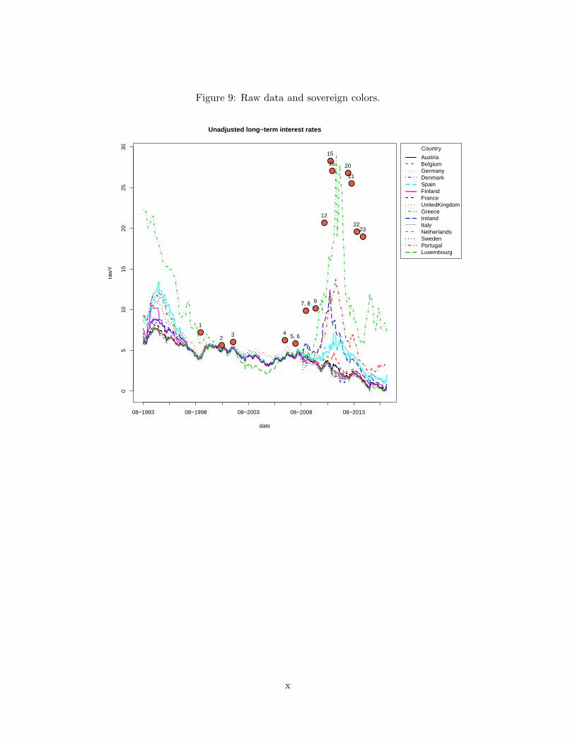
Figure 9: Raw data and sovereign colors.

05

1015

2025

30Unadjusted long−term interest rates

date

raw

Y

08−1993 08−1998 08−2003 08−2008 08−2013

Country

AustriaBelgiumGermanyDenmarkSpainFinlandFranceUnitedKingdomGreeceIrelandItalyNetherlandsSwedenPortugalLuxembourg

1

2 3 4 5, 6

7, 8 9

12

15

16 20

21

2223

x

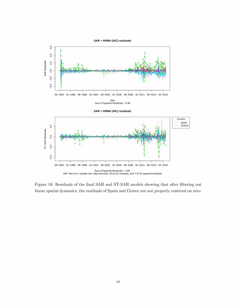
−0.

4−

0.2

0.0

0.2

0.4

0.6

SAR + ARMA (AIC) residuals

Sum of Squared Residuals = 8.38date

SA

R R

esid

uals

08−1993 02−1996 08−1998 02−2001 08−2003 02−2006 08−2008 02−2011 08−2013 02−2016

−0.

4−

0.2

0.0

0.2

SAR + ARMA (AIC) residuals

Sum of Squared Residuals = 3.95 DM−Test on in−sample one−step forecasts, 20.01 for residuals, and 7.37 for squared residuals.

ST

−S

AR

Res

idua

ls

08−1993 02−1996 08−1998 02−2001 08−2003 02−2006 08−2008 02−2011 08−2013 02−2016

Country

SpainGreece

Figure 10: Residuals of the final SAR and ST-SAR models showing that after filtering out

linear spatial dynamics, the residuals of Spain and Greece are not properly centered on zero.

xi

5 10 15 20

−0.

20.

00.

20.

4

ACF of SAR + ARMA (AIC) residuals

Lags

AC

F

0.95 level individual significance bound0.95 level Bonferonni significance boundcomplete range of cross−sectional ACF valuesmedian of cross−sectional ACF values

5 10 15 20

−0.

20.

00.

20.

4

PACF of SAR + ARMA (AIC) residuals

Lags

Par

tial A

CF


5 10 15 20

−0.

20.

00.

20.

4

ACF of ST−SAR (AIC) + ARMA (AIC) residuals

Lags

AC

F


5 10 15 20

−0.

20.

00.

20.

4

PACF of ST−SAR (AIC) + ARMA (AIC) residuals

Lags

Par

tial A

CF


Figure 11: Residual correlations of the SAR and ST-SAR.

xii

Timeline of events related to European Long term Interest

Rates

1 January 1999, start of the Euro;

2 January 2001, Greece joins the Euro;

3 January 2002, Euro coins and notes are introduced;

4 January 2007, Slovenia joins the Euro;

5 January 2008, Malta and Cyprus join the Euro;

6 November 26, 2008, 200bn European Economic Recovery Plan;

7 January 2009, Slovakia joins the Euro;

8 January 2009, Estonia, Denmark, Latvia and Lithuania join the ERM;

9 December 17, 2009, Greece hits deficit record;

10 April 19, 2010, Greece hits borrowing cost record;

11 May 2, 2010, Greece accepts 110bn bailout package;

12 November 28, 2010, Ireland accepts 85bn bailout package;

13 January 2011, Estonia joins the Euro;

14 February 14, 2011, agreement of 500bn ESM bailout fund;

15 May 3 , 2011, agreement over 78bn bailout package for Portugal;

16 July 21, 2011, agreement over additional 109bn bailout package for Greece;

17 October 6, 2011, Bank of England to inject an additional 75bn pounds into the economy;

18 January 2012, major downgrade wave including nine Eurozone nations by S&P;

19 June 2012, Spain and Cyprus request assistance from the ESM;

20 January 23 2013, England threats to leave the European Union;

21 May 2, 2013, ECB cuts the rate on its benchmark refinancing facility to 0.50%;

22 November 7, 2013, ECB cuts the rate on its benchmark refinancing facility to 0.25%;

23 June 2014, first negative interest rates by the ECB;

24 June 23, 2016, Brexit.

xiii

Smooth Transition Spatial Autoregressive Models · 2017-05-30 · Smooth Transition Spatial...

Documents

Transcript of Smooth Transition Spatial Autoregressive Models · 2017-05-30 · Smooth Transition Spatial...