Smooth-Adjustment Econometrics and Inventory-Theoretic Money Management

Clinton A. Greene* Department of Economics

University of Missouri-St. Louis St. Louis, MO 63121-4499

(314) 516-5565

fax (314) 516-5352 clinton_greene@umsl.edu

November, 2009

Abstract A growing number of empirical papers use Miller-Orr (S, s) money management as economic motivation for application of non-linear smooth-adjustment models. This paper shows such models are not implied by the Miller-Orr economy. Instead, the Miller-Orr economy implies non-standard smooth-adjustment, as derived in the neglected (and misinterpreted) work of Milbourne, Buckholtz and Wasan (1983). Remarkably, this function includes a varying weight on the lagged dependent variable, capturing static (not dynamic) effects. Interpretations of these apparent dynamics are presented, some of which may be useful in non-monetary (S, s) contexts. Results imply a new agenda for applied smooth-adjustment modeling of money.

JEL: C22, E41, B22 Key Words: Money; Miller-Orr; Smooth-Adjustment; Nonlinear; Inventory.

* Department of Economics, University of Missouri-St. Louis, St. Louis, MO 63121-4499, Tel (314) 516-5565, Fax (314) 516-5352, Email address: clinton_greene@umsl.edu

1

0. Introduction

Non-linear smooth-adjustment models as developed by Terasvirta (1994) have been

applied to monetary data in a growing number of empirical studies. Where authors have offered

motivation from monetary theory for these non-linear methods they have always made reference

to target-threshold (or trigger-target, or S,s) money management rules based upon inventory

theory, with most referring to the Miller-Orr variant. This is natural, as Miller-Orr style money

management induces complex behavior, and smooth-adjustment models employ very flexible

non-linear functional forms.

The Miller-Orr monetary model is cited as underlying motivation for smooth-adjustment

econometrics applied to Italian data in Sarno (1999), for Taiwan in Huang, Lin and Cheng

(2001), to Spanish data in Ordonez (2003), and for US data in Sarno, Taylor and Peel (2003).

The most detailed argument for this economic rationale is provided in Sarno’s 1999 paper and

again in Sarno, Taylor and Peel (2003). Other papers using Miller-Orr as economic motivation

for smooth-adjustment either refer to or reproduce elements of their argument. These more

recent papers include Chen and Wu (2005) who investigate both US and UK data, Lee, Chen and

Chang (2007) for G-7 data, US data again in Haug and Tam (2007), and then data for Taiwan in

Wu and Hu (2007) and again in Lee and Chang (2008).1

The argument made for a tie between smooth-adjustment and the Miller-Orr economy is

based upon the fact that under the Miller-Orr rule (and under inventory-theoretic models in

general) the individual agent allows the balance to wander as driven by random net receipts, and

adjustment to a target level is triggered only if the balance breaches upper or lower bounds of

1 Via the SCOPUS data-base it was found that the works in this list of papers (claiming a Miller-Orr rationale) were in turn cited in eighteen other published papers, nine of these in 2007 through 2008. Among the eighteen, ten cite Sarno (1999) or Sarno, Taylor and Peel (2003).

2

some interval. It is taken as intuitively obvious that the larger the deviation of holdings from the

long-run (or average, or equilibrium) value then the more likely it is that many accounts are close

to breaching their trigger-points, soon to adjust towards the targets. Thus the deviation of

holdings from their long-run levels should affect the speed of adjustment towards this long-run,

with the speed of adjustment increasing with the size of the aggregate deviation. It is then noted

that smooth-adjustment functions allow for just such a positive relationship between (on the one

hand) deviations from equilibrium and (on the other hand) the speed of adjustment. On that

basis these papers claim it is intuitively obvious that Miller-Orr money management must imply

smooth-adjustment.2

This paper shows that some of this intuition is correct, but a Miller-Orr economy induces

important complications not captured in the standard smooth-adjustment functional forms.

Consistent with the applied literature, the Miller-Orr economy is non-linear, and in a Miller-Orr

economy standard smooth-adjustment functions can improve on the fit of linear models. But not

for the reasons described in this literature. This paper also shows the standard smooth-

adjustment representations of the Miller-Orr economy are unstable (in a Miller-Orr economy)

and so forecast poorly. This instability is not a function of time, so may not be detected when

applying standard stability tests. Anticipating the dimension along-which this instability lies and

specifying a stable non-linear function requires considerations additional to those discussed in

this monetary smooth-adjustment literature.

In clarifying the issue it will be useful to compare the smooth-adjustment intuitions to

some prior results neglected in the literature. Milbourne, Buckholtz and Wasan (1983, hereafter

MB&W) presented rigorous results on the form of aggregate non-linearity implied by Miller-Orr

2 Motivation from buffer-stock models is also mentioned. A buffer-stock is an inventory, and inventory optimization leads to (S,s) rules, so it is not clear that buffer-stock theory is distinct from Miller-Orr type thinking.

3

money management. But their results are not incorporated into any of these published papers

applying smooth-adjustment econometrics.3 And their results have generally been neglected.

The correct non-linear model derived by MB&W is a non-standard smooth-adjustment model

with a static transition variable. The use of a static rather than a dynamic transition variable sets

the correct model apart from the standard smooth-adjustment approach.

The fact that rigorous results for the non-linear nature of the Miller-Orr economy

(derived by MB&W) have been largely ignored for a quarter-century is a puzzle in itself worth

addressing. In my view there are two legitimate reasons for the neglect. First, the discussion in

MB&W is very brief and does not provide a helpful description of the nature of their

mathematical results. Second, their most precise results are buried among other loose

approximations adopted for empirical application, necessitated by the limited computing power

available at the time. Given these handicaps, it is not surprising that non-linear modeling of (S,

s) economies has been little affected by their work.

In response to these difficulties, I present descriptions and intuitive heuristics useful for

understanding the work of MB&W. Since (S, s) models have application not only in inventory

management but also in some (New-Keynesian) price-adjustment modeling, some of the

interpretation presented in this paper will be more broadly useful. So along the way I comment

on which results here are likely to hold in other contexts and which characteristics are unique to

money.

The paper proceeds in six steps. Section 1 discusses how a Miller-Orr economy implies

(in the aggregate context) a model with the structure of partial-adjustment (or restricted error-

correction), but with weights or coefficients which vary. In this initial discussion it will become

apparent that the probability of portfolio adjustment does matter for coefficient values. Hence an 3 Although cited by Sarno (1999), the actual results of MB&W are not discussed nor used.

4

aspect of the motivation for application of smooth-adjustment models to money data adopted in

the applied literature is indeed correct.

In Section 2 simulation methods are used to investigate how well standard smooth-

adjustment and related forms can model this varying probability as posited in the monetary

smooth-adjustment literature, namely that this probability is a function of the difference between

actual and expected money holdings. It turns out that such functional forms do no better than

assuming a constant probability. This means that if smooth-adjustment models perform well

empirically, then this is not due to this aspect of the story told in the literature.

The difficulty with the story is due to the fact that under aggregation money holdings can

be larger than average without individual holdings lying closer than usual to the upper boundary

of the (S, s) interval. To support intuition for the simulation results I provide a counter-example

which can easily be extended to a continuum of variations. This result is the most likely to carry

over into other non-monetary contexts.

In Section 3 I turn to the derivations of MB&W, showing that although their results can

be seen as implying a highly modified smooth-adjustment model, the form is not the one used in

the smooth-adjustment literature (to date) and the theoretical interpretation is quite different. In

particular the standard smooth-adjustment model is telling a dynamic story. But although the

non-linear MB&W model incorporates a lagged dependent variable, it is nonetheless a model of

comparative statics.

That trigger-target (S, s) behaviors at the individual level can imply for an aggregated

model that lagged money is important, but this lag is not capturing dynamic effects, is perhaps

the key insight into the nature of a monetary (S, s) economy. Likewise non-linearity is generated

in a comparative-statics context. Once one understands the static basis for non-linearity (and the

5

predictive role of lagged money despite the static context), it becomes possible to understand

how standard smooth-adjustment forms can approximate a Miller-Orr economy, but for reasons

not yet discussed in the literature. Standard smooth-adjustment forms may be approximating

comparative static effects of the Miller-Orr economy rather than capturing dynamics.

This leads in Section 4 to consideration of a different sort of simulated Miller-Orr

economy, one in which comparative statics are central (and of large magnitude). There I

compare standard “dynamic” smooth-adjustment models and a model based upon MB&W. It

will turn out that all the models are close competitors when fitting within sample. In the non-

linear Miller-Orr economy there is little difference in fit between standard smooth-adjustment

models, the MB&W model, and even linear models. But smooth-adjustment models equivalent

to those estimated in the monetary literature (to date) are highly unstable in this Miller-Orr

economy, forecasting out-of-sample with much larger (mean-squared) errors than those for the

MB&W model. For reasons that will become obvious the relevant test of stability is not with

respect to time, but rather stability with respect to the level of the variable driving the non-

linearity, introduced in the next section.

Sections 5 and 6 discuss issues in empirical application of the correct non-linear

(MB&W) model and present a short empirical application in US quarterly data, comparing it to a

log-linear model. Although the MB&W form is much simpler than standard smooth-adjustment

models, it cannot be applied directly to the aggregate data usually employed in applied studies.

Suggestions are made for approaching these issues which may be helpful in applying the model

to data considered elsewhere in the smooth-adjustment literature, such as non-US data or annual

series for the nineteenth century. Although keeping this paper to reasonable length requires an

6

abbreviated empirical treatment, I make some effort to outline questions that deserve more

extensive empirical investigation elsewhere.

1. Predictors of Money Holdings in the Miller-Orr Economy

The Miller-Orr monetary model is one example of the class of inventory-theoretic models

which take account of the fact that lumpy costs of exerting control imply it is optimal to allow

the controlled variable to wander as driven by daily events (such as receipts and disbursements,

or sales and deliveries), exerting control only when the variable breaches some interval. Such

optimal control models (sometimes called (S, s) or trigger-target models) are routine in

engineering and business, and most of the relevant literature long ago migrated to the business

and optimal-control journals.4 A general model developed in the contemporary economics

literature is found in Bar-Ilan, Perry and Stadje (2004).

A Miller-Orr agent finds it optimal to adopt a two-sided (S, s) rule, allowing the money

balance to wander randomly within bounds. This policy of letting the balance wander within

some interval is optimal given fixed (lumpy) costs of transfers between money and the

alternative interest-bearing asset.5 In the most common formulation the costs of a negative

balance are implicitly taken to be greater than the lumpy transfer cost, implying a lower bound of

zero and a management interval of [0,H]. The standard model familiar to economists assumes

4 Applications can be very complex. For instance, banks now avoid reserve requirements on about half of freely-checkable deposits by using software that periodically transfers funds between the depositor’s account and a “shadow” or “accounting” money market deposit account (MMDA). In any month only six withdrawals are permitted, hence a seventh has a large and lumpy cost, inducing a non-linear optimal control problem with time-varying targets and triggers (S,s). 5 There are counter-examples to optimality in the economics literature which rely on imposition of additional conditions. For instance, the counter-example in Bar-Ilan (1990) relies on imposing a zero balance in a final period, implying the holding cost of money in the final period is not only different than in previous periods but must be unbounded (undefined) for a non-zero balance. More general optimality results which make reference to the traditional transactions models familiar to economists can be found in Constantinides and Richard (1978), Vickson (1985) and Bertola and Caballero (1990).

7

daily net receipts are discrete and independent draws of positive or negative one, but the same

optimality results hold if the balance follows a symmetric discrete or continuous (diffusion)

process, and/or under continuous monitoring. In such cases there is a single optimal target Z =

H/3. In these standard formulations the distribution of the balance is triangular, with a mean m =

4H/9 which one should note is greater than the target Z (=H/3). The value of the upper trigger

(H) will depend on the expected yield on the alternative asset and the variance of daily net

receipts. Such considerations affect scaling but not the shape of the distribution nor the

relationships between optimal Z, H and expected holdings.

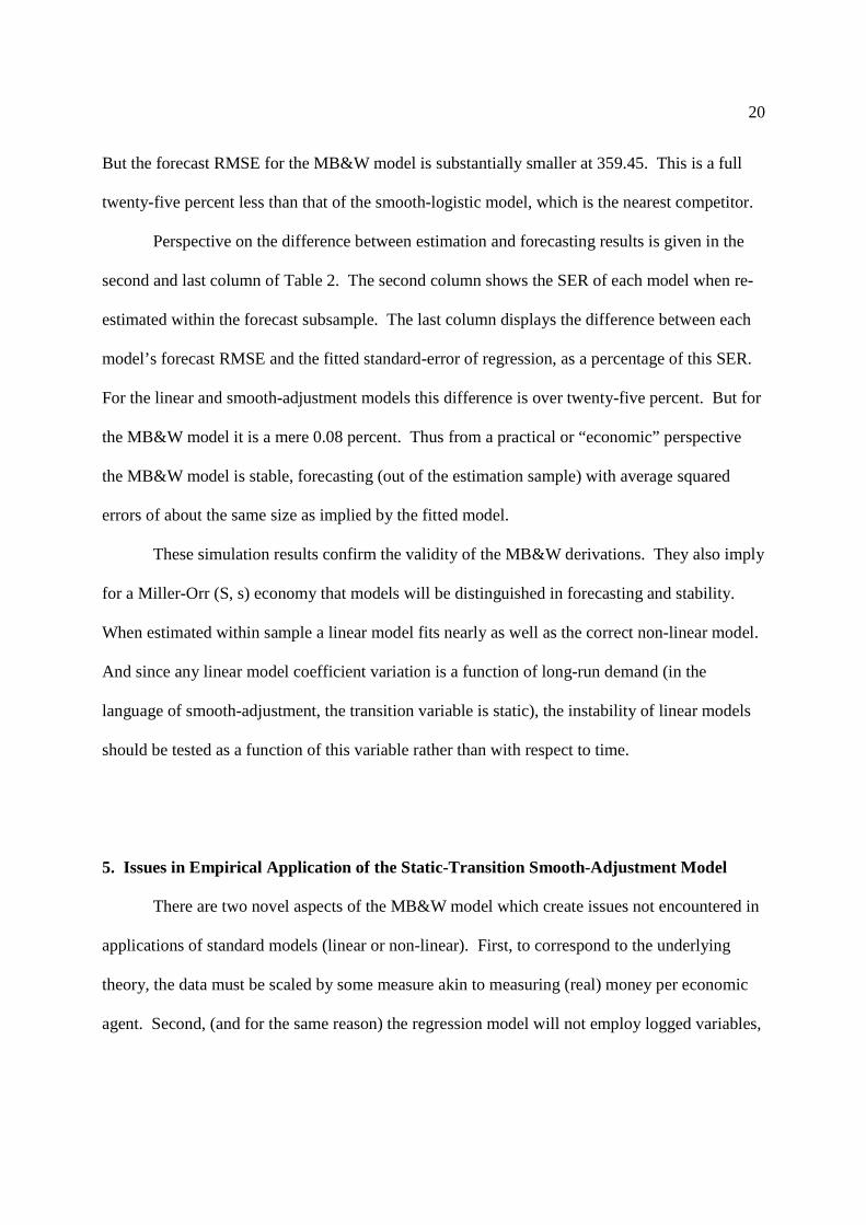
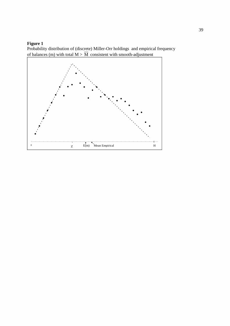
Because individual holdings are random, the empirical distribution of balances for an

economy of n accounts will differ at any point in time from the probability distribution. Taking

Mt as the actual total at time t and denoting the aggregate expectation as M =nm , then the

difference Mt - M is itself random. Figure 1 shows the triangular distribution and illustrates a

possible empirical frequency, this distinction is important both for the role of lagged holdings

and the smooth-adjustment intuition.

1.1 Mean Holdings or “Long-Run Demand”

The usual approach to application of Miller-Orr type models uses only expected holdings

or for an economy of n accounts

tM = M . (1)

The inventory-theoretic literature often refers to the expectation M as “long-run demand”,

“desired holdings” or simply “demand”. The use of the term “desired” is unfortunate, since all

levels of holdings within the management interval are optimal, and strictly speaking demand is a

correspondence not a function. The use of the term “target” for the value Z is likewise

8

unfortunate, since this value is optimal only infrequently (at the moment of a decision to change

holdings), and for inventory based models in general the expected value of holdings does not

correspond to this “target” level.6

1.2 Lagged Money as a Static Predictor

The most interesting properties of the Miller-Orr economy derive from the fact that as

long as an individual balance has not breached the management interval then it wanders

randomly as driven by net receipts over time. This implies there is an important alternative to

using the simple mean tM as a predictor. In particular, from one observation of money to the

next a portion of account balances have not been interfered with, having followed a random walk

without encountering the bounds [0, H]. This implies we could also use an alternative predictor

based upon the random walk property or

'tM = Mt-1. (2)

This might seem to be poor competitor with the mean M , especially since we may be observing

money infrequently and balances may have wandered far from their previous (time t-1) values.

However for a closed model these transactions receipts must net to zero, and within the subset of

accounts not breaching their management intervals many will have transacted mostly with like

accounts, and thus the net change in holdings for these accounts is close to zero. The sum of

holdings from time t-1 to t is modified only to the extent portfolio readjustments have been

6 To have z = m , in the Miller-Orr case requires z =H/2. This point applies to more general models which have two targets (depending on whether the upper or lower bound is breached), each of which differs from mean holdings.

9

triggered.7 If there are proportionally few portfolio rearrangements, then 'tM can have a much

lower error variance than the alternative tM .

This strong and static role for lagged money need not carry over to other (S, s) contexts.

In a closed monetary model each transactions credit implies a balancing debit. But physical

inventory models do not generally include an analogous condition, because natural resource

extraction is not usually counted as a decrease in inventory, and household inventory

accumulations are also usually neglected.8 And in menu-cost driven pricing models an increase

in one firm’s price is not taken to imply a decrease in the prices or costs of another. Hence a role

for the lagged dependent variable is special to monetary models.

1.3 The Nesting Model and Non-Linear Weighting

We have two predictors based upon very different considerations, one relying upon the

unconditional mean and one which is informative for a subset of accounts. We can improve our

forecasts by using a pooled or joint model. Hence in a Miller-Orr economy a model with lower

error-variance than (1) and (2) is

Mt = bMt-1 +(1 -b)M +εt. (3)

In applications one would date the unconditional mean tM , in which case the error-correction

form would be (using the traditional equilibrium-correction term Mt-1 - 1-tM )

∆M t = (b-1)(Mt-1 - 1-tM - tM∆ ) +εt . (4)

7 This also implies the assumption of a random walk in net receipts is not necessary. But straying from this assumption leads to more complex optimization problems than in the Miller-Orr case, and also leads to difficulties in satisfying the aggregation condition that a transactions receipt for one agent must be a debit for another. 8 It might be possible to include this element in a physical inventory model which allows for multiple layers of intermediate processing and production, where an increase in one firm’s inventory would be provided by a decrease in the inventory held by the supplying firm.

10

But the unique aspects of the Miller-Orr economy are most starkly illustrated if we assume

management intervals thus M are constant (implicitly holding the interest rate constant).

Because the timing of management interval breaches is random, the random component is

inherent in the Miller-Orr world, and Equation 3 applies even with a constant unconditional

mean(M ). And the derivations of Milbourne, Buckholtz and Wasan discussed in Section 3

make this assumption of a constant mean. In this case we can remove the time subscript from

M ( tM = 1-tM ) and simply write Equation 3 as

∆M t = (b-1)(Mt-1 - M ) +εt . (5)

Nonlinear models arise as forms which allow this weight to vary. The smooth-

adjustment intuition relies upon a connection between the probability of asset transfers (breaches

of [0,H]) and the value of the weighting b. It is important to note that in partial-adjustment it is

legitimate to speak of M as a desired level towards which holdings adjust. But in a Miller-Orr

economy random holdings are inherent in individual behavior, there is no single-valued optimum

and so it is misleading to think of the weight (b) as measuring a speed of adjustment.

Put differently, partial-adjustment is a dynamic story. But in our Miller-Orr economy it

will be more useful to think of Equations 3, 4 and 5 as employing alternative static predictors,

despite the presence of a lag of money. Rather than interpreting a large weight on lagged money

as indicating slow adjustment, a more accurate heuristic is to think of it as implying lagged

holdings are informative for a large portion of agents because portfolio readjustments are

infrequent.

11

2. The Smooth-Adjustment Interpretation of the Miller-Orr Economy

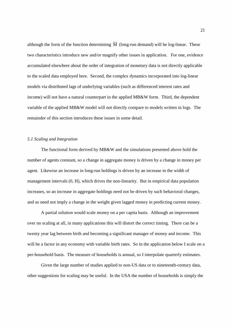
In Figure 1 the actual distribution of accounts is skewed more towards the upper bound

(H), than is implied by the triangular probability distribution. This has two implications. First,

actual holdings are greater than the mean predicted by the probability distribution i.e. Mt - M >0.

Second, since balances are more concentrated near the upper threshold H, from t to t+1 there is a

greater than usual probability of asset transfers (restoring more balances to Z), and hence a

greater probability than usual of a reduction in total holdings.

The smooth-adjustment story takes a positive difference between actual and mean

holdings as a signal that breaching the upper bound of the management interval is more likely

than usual. Thus the smooth-adjustment intuition leads us to allow the weighting in the above

equations (b) to vary over time as a function of Mt -M :

∆M t = (bt-1)(Mt-1 - M ) +ε’ t (6)

bt =f(Mt-1 - M )

In the monetary smooth-adjustment literature the function f() has been taken to be of two

possible forms, exponential or logistic, with (respectively) bt = exp[-c2(Mt-k - M -c3)2] or bt = 1 -

1/[1 +exp(-c2(Mt-k - M -c3))], where c2>0 and we avoid notational clutter by letting the

coefficients ci have different values across equations. Most applications also allow for a linear

(fixed) component and may add an additional scaling factor or bt = b0 +b1* f(Mt-1 - M ). Some

studies have investigated other transition variables but have usually rejected them in favor of

(M t-1 - M ). In any case this is the transition variable consistent with the intuition claimed to

motivate a Miller-Orr basis for smooth-adjustment models.

12

2.1 Does the Smooth-Adjustment Story Work?

The question is whether knowing the difference between actual and mean holdings tells

us something about the probability of asset transfers. Here I take a direct approach, simulating a

Miller-Orr economy, recording the portion of accounts engaging in transfers (pt) from time t-k to

t and also recording (Mt-k - M ), where M = the expectation implied by the triangular

distribution. I then try to model pt as various functions of (Mt-k - M ). If k >1 then values are

recorded every k’th period. For given (Z, H) the implied weight on lagged money in Equation 3

decreases as the time between observations (k) increases.9

In the simulations there are 20,000 accounts which are randomly paired each period and

receive a debit or the balancing credit. An important aspect of such a model is that the timing of

management interval breaches (or asset reallocations) will be random and thus in the aggregate

unbalanced. Without Central Bank commitment to provide liquidity as needed, it is not possible

to hold interest rates and thus management intervals constant. So to the extent portfolio

readjustments are triggered, the simulations implicitly treat any imbalances as met by Central

Bank commitment to stabilizing interest rates. This implies aggregate holdings vary randomly

over time.

The simulations are long enough to generate one-thousand observations (regardless of

observation frequency k) of Mt and Mt-k for a given z and thus for a constant M . This was done

for all combinations of k = 1, 2, 3, 4, 5, 10, 15, 20 and z = 5, 10. Results were similar in all cases,

in the case presented (k = 10, Z = 10) the average estimated value for the weight on lagged

money in a regression of Equation 1 is about 0.8.10

9 This is discussed in Section 3. 10 Programs and resulting data files are available upon request.

13

Table 1 shows the results of attempts to model pt using various forms related to the

smooth-adjustment story. The second column from the right shows the results of a test for

restricting the model to a constant, showing the probability value of a simple ANOVA F-statistic.

Since these are large samples, a very small change in the model variance (restricted versus

unrestricted) could still at conventional significance levels lead to rejection. So in the last

column on the right I display the coefficient of variation for the models. Since this (R2) is zero

when the constancy restriction is imposed, it is a measure of the gain of the non-linear model

over the linear model.

The first row of Table 1 shows the results of attempting to model the portion of accounts

breaching the management bounds using a smooth-exponential model.11 The probability value

for imposition of a constant relationship is 0.0582, implying rejection for a test size of ten-

percent, but not for a size of five percent. Given the large sample it makes sense to choose a test

size smaller than conventional values, i.e. a size well under five-percent. More to the point, in

the last column we find the R2 of this smooth adjustment form is 0.00748, well under one

percent. Very little of the variation in the rate of portfolio adjustment (pt) is explained by this

smooth-exponential function.

The second row of Table 1 shows results for a smooth-logistic function. Here we can

accept the restriction to a constant, the probability value for the implied restriction being 0.388.

The third and fourth rows investigate alternatives to the standard smooth-adjustment forms,

attempting to model pt as a function of the absolute value of the transition variable (Mt-1 - M ).

Again the cost in reduced fit when reverting to the intercept-only model is small, and the implied

restrictions are not rejected.

11 I do not impose sign restrictions.

14

This aspect of the smooth-adjustment intuition has failed, knowing Mt-1 ≠ M does not

help us predict the probability of adjustments to target levels. What then is wrong with the

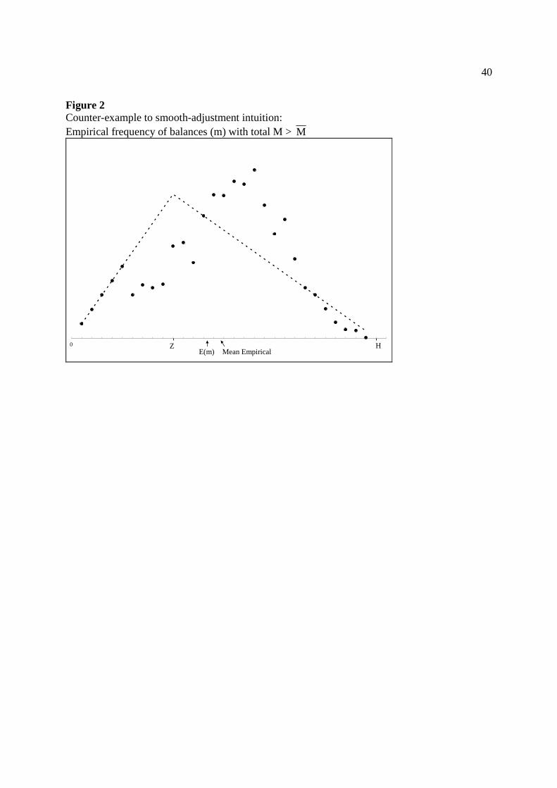
smooth-adjustment intuition? The answer is simple, and is illustrated in Figure 2. As in Figure

1, here actual holdings are greater than M . But the probability of near-term breaches of the

interval is not greater than usual, because the actual density of balances near the bounds 0 and H

is not greater than usual. In fact the portion of balances near the upper bound is lower than

usual, implying a lower probability of reductions in balances despite average holdings greater

than the long-run mean (M >M ). For an individual balance it is correct that mt - m >0 implies

mt is closer to H than usual. But this does not hold for an aggregate distribution. It is easy to

imagine a continuum of similar counter-examples with varying empirical distributions. The

simulations tell us that the sort of distribution illustrated in Figure 1 is no more likely than that

illustrated in Figure 2.

In these simulations we were holding the management interval width (0, Z, H) constant,

so any variation in the rate of portfolio adjustment was due to short-term dynamic fluctuations in

the empirical density away from the theoretical distribution, as posited in the smooth-adjustment

literature. It turns out that although this aspect of the smooth-adjustment intuition is not correct,

there are other reasons for a gain in moving from linear to smooth-adjustment models. But to

discuss these reasons it will first be helpful to examine the results of MB&W.

3 Milbourne, Buckholtz and Wasan: Nonlinear Aspects of the Miller-Orr Economy

MB&W formally derive the optimal relative weighting (b or bt in Equations 3-6) as a

function of the width of management intervals, the variance of daily net receipts, and the time

elapsing (k) between observations of money. For our purposes the most useful result is their

15

Equation 20. We will be holding constant the variance of daily net receipts and the elapsed time

between observations of money (respectively σ2 and t in MB&W). Folding constants into one

term and also taking advantage of the fact that M =nm = n4h/9 (they denote the upper threshold

with the lower case “h”), then we can rewrite their result for the weighting as

b = exp(c0/ M 2) c0 < 0. (7)

3.1 Interpreting the Milbourne, Buckholtz and Wasan Model

It is important to note that in Equation 7 I have not given mean or long-run holdings (M )

a time subscript, as the problem solved by MB&W takes the management interval (0, Z, H) and

thus long-run holdings as a given. Thus their result is static from two perspectives. Their task is

a comparative statics exercise in the sense that Equation 7 shows how the optimal weighting will

differ in Equations 3-6 across separate regimes in which long-run demand is constant but takes

on different values across the regimes. Their result does not tell us about the transitions between

regimes, for instance it does not tell us about the effects occurring during a reduction in the upper

threshold H (say in reaction to higher interest rates) as the process of compressing the

distribution of Figure 1 piles probability mass at the target (Z). Such dynamics are complex and

transitory, and are not addressed by Equation 7 nor by MB&W.12

Their result is static in a second respect. If Equation 7 was a smooth-adjustment function

then the right-hand side transition variable would be the dynamic difference Mt-1 - M .13 Due to

the random nature of Miller-Orr holdings this varies from moment to moment even when

12 Greene (2001) explores the very complex nature of Miller-Orr dynamic transitions and develops modifications of the non-linear comparative-static MB&W model to allow for these dynamics. 13 Another possibility in smooth-adjustment modeling is to use a transition variable formed as changes of some of

the variables determining demand, if not ∆ M then changes in interest rates or changes in income. In this case the characterization of smooth-adjustment as dynamic and the MB&W model as static still applies.

16

management intervals and M are constant. So smooth-adjustment implies a varying coefficient

(b) when management intervals and long-run demand are constant. But Equation 7 employs the

level of long-run demand and if long-run demand is constant then the equation and the MB&W

results imply a constant weighting.

Unfortunately the discussion in MB&W can be unhelpful. Their use of terms is entirely

proper if one defines short-run adjustment as being involved anytime a model includes a lagged

dependent variable. But as we have seen above their mathematics assumes away most of what

would usually be considered dynamic, and so “comparative-statics” is a more useful label. If

one reads carefully one can tease out some of this static-dynamic distinction, for instance they

state that “this view of money holdings is different from the usual stock adjustment view” and

they refer to the distribution of holdings “whose average is the ‘desired’ level of money

holdings.” Yet at times they refer to their results as regarding the “short-run” and “adjustment”.

Also, their theoretical section essentially ends with Equation 21. The later equations are

motivated by an effort to take shortcuts for empirical application. For instance they abandon the

exponential form implied by their results, moving to a simpler Taylor series approximation.

Such simplifications are understandable given the computing power available at the time, but are

unnecessary today. They also assume some proxies for the variance of daily receipts and for

portfolio adjustment costs which deserve more careful examination. So those contemplating

empirical applications will stand on the strongest theoretical ground if they take inspiration from

MB&W’s Equations 20 or 21.

17

4. Smooth-Adjustment and Comparative Statics

The work of MB&W implies non-linearity emerges in the comparative statics context,

with differing regimes of management interval width. Although the results above show that

smooth-adjustment cannot be justified on the basis claimed in the literature, this does not rule out

the possibility that smooth-adjustment can well approximate a Miller-Orr economy with

differing regimes, a factor not included in the simulations above. There is the additional

consideration that smooth-adjustment functions are very flexible forms, and the form derived by

MB&W relies upon truncation of some expressions and is more restrictive than standard smooth-

adjustment. Thus it is of interest to compare smooth-adjustment functions to the MB&W form in

a comparative statics context.

This section examines the performance of linear, smooth-adjustment, and the MB&W

forms in a Miller-Orr economy in which management intervals and mean holdings differ over the

sample, making comparative static effects operative. Again the simulated economy will consist

of 20,000 accounts. But here there are 14 regimes of differing management intervals with

parameters chosen so the implied weight on lagged money (b or bt of Equations 3-7) varies as

(approximately) 0.30, 0.35, 0.40, ...0.95. In order to achieve this design I make two related

changes to the previous simulations. Net receipts are drawn from a normal (0,1) distribution, and

parameters Z and H are allowed to equal non-integer values.14 For each of the fourteen regimes I

record ten-thousand observations of aggregate M, Mt-k, and M t, for a total of 140,000

observations.

14 This is equivalent to assuming balances follow a diffusion process. As shown in MB&W, this maintains the mean (and optimality results) of the original discrete framework of Miller and Orr.

18

4.1 Within-Sample Fit, Stability and Out-Of-Sample Forecasting

All of the competing models are variations of

Mt = btMt-1 +(1 -bt) M t +εt bt =f(.) (8)

where M is not estimated but is the population value 20000(4H/9). In the linear model bt is a

constant to be estimated directly. As in standard practice the smooth-adjustment models are

specified to nest the linear case. For the smooth-exponential model f(.) is replaced by

c0 +c1exp[-c2(Mt-k - tM -c3)2], while for the logistic versions f(.) is replaced by

c0 -c1/[1 +exp(-c2(Mt-k - tM -c3))]. For the MB&W model f(.) is replaced by exp(c0/2tM ).15 The

coefficients (ci) are estimated via simple non-linear least-squares. It is helpful to recall that Mt

varies randomly from observation to observation, but tM is constant (via constant management

interval width) over sub-samples of 10,000 observations.

4.2 Within-Sample Fit

The second column of results in Table 2 shows the regression standard errors when fitting

the models in the half of the simulated data in which management intervals (and mean holdings)

are larger (b = 0.65, ...0.95). Notice the linear model SER of 365.43 a bit larger but very close to

the smooth-adjustment model SER’s of 364.00 and 364.57 and also close to the SER of the

MB&W model (359.16). In fitting within sample the linear model is able to approximate

comparatively well even though we know coefficients vary. Likewise there is little to

distinguish among the non-linear model standard-errors.

15 Where for notational simplicity coefficients ci represent different values across equations.

19

4.3 Forecasting and Stability in the Miller-Orr Economy

In these large samples (70,000 observations) one could reject constant model coefficients

even if coefficient variation is too small to be of importance. As discussed in DeGroot (1986,

pp496-7) one way to deal with this it to decide how small a difference matters, and adjust the test

size to avoid rejection of differences judged to be small. But unless one knows the results ahead

of time, this requires ex-post examination of estimated variances in order to pick the useful test

size.

I take a more direct approach. Since all the models fit nearly as well within a sample of

varying regimes, instability will be important only if one is forecasting for a regime not included

in the estimation sample. And we can obtain a measure of the importance of such instability by

fitting and forecasting in distinct sets of regimes. Thus forecasting “out of sample” will give us a

measure of the importance of any instability.

The first column of results in Table 2 shows the results of this sort of forecasting

exercise. In particular, we are forecasting for the same set of data used to estimate regression

standard errors in the second column. But the forecasts here use coefficients as estimated in the

other half of the data, data in which Z and H have taken values outside the range of those within

the data being forecast. In particular I estimate coefficients over the 70,000 observations in

which (Z, H) vary to imply an optimal linear weight on lagged money that varies as 0.30, 0.35,

...0.60, and then forecast over the next 70,000 observations in which (Z, H) imply a linear weight

varying as 0.65, 0.70, ...0.95. Thus the sample is divided not by time, but by mean holdings M .

For the linear model the forecast RMSE is 467.68, a bit smaller than that for the smooth-

exponential model of 472.05, but larger than the RMSE of 452.84 of the smooth-logistic model.

20

But the forecast RMSE for the MB&W model is substantially smaller at 359.45. This is a full

twenty-five percent less than that of the smooth-logistic model, which is the nearest competitor.

Perspective on the difference between estimation and forecasting results is given in the

second and last column of Table 2. The second column shows the SER of each model when re-

estimated within the forecast subsample. The last column displays the difference between each

model’s forecast RMSE and the fitted standard-error of regression, as a percentage of this SER.

For the linear and smooth-adjustment models this difference is over twenty-five percent. But for

the MB&W model it is a mere 0.08 percent. Thus from a practical or “economic” perspective

the MB&W model is stable, forecasting (out of the estimation sample) with average squared

errors of about the same size as implied by the fitted model.

These simulation results confirm the validity of the MB&W derivations. They also imply

for a Miller-Orr (S, s) economy that models will be distinguished in forecasting and stability.

When estimated within sample a linear model fits nearly as well as the correct non-linear model.

And since any linear model coefficient variation is a function of long-run demand (in the

language of smooth-adjustment, the transition variable is static), the instability of linear models

should be tested as a function of this variable rather than with respect to time.

5. Issues in Empirical Application of the Static-Transition Smooth-Adjustment Model

There are two novel aspects of the MB&W model which create issues not encountered in

applications of standard models (linear or non-linear). First, to correspond to the underlying

theory, the data must be scaled by some measure akin to measuring (real) money per economic

agent. Second, (and for the same reason) the regression model will not employ logged variables,

21

although the form of the function determining M (long-run demand) will be log-linear. These

two characteristics introduce new and/or magnify other issues in application. For one, evidence

accumulated elsewhere about the order of integration of monetary data is not directly applicable

to the scaled data employed here. Second, the complex dynamics incorporated into log-linear

models via distributed lags of underlying variables (such as differenced interest rates and

income) will not have a natural counterpart in the applied MB&W form. Third, the dependent

variable of the applied MB&W model will not directly compare to models written in logs. The

remainder of this section introduces these issues in some detail.

5.1 Scaling and Integration

The functional form derived by MB&W and the simulations presented above hold the

number of agents constant, so a change in aggregate money is driven by a change in money per

agent. Likewise an increase in long-run holdings is driven by an increase in the width of

management intervals (0, H), which drives the non-linearity. But in empirical data population

increases, so an increase in aggregate holdings need not be driven by such behavioral changes,

and so need not imply a change in the weight given lagged money in predicting current money.

A partial solution would scale money on a per capita basis. Although an improvement

over no scaling at all, in many applications this will distort the correct timing. There can be a

twenty year lag between birth and becoming a significant manager of money and income. This

will be a factor in any economy with variable birth rates. So in the application below I scale on a

per-household basis. The measure of households is annual, so I interpolate quarterly estimates.

Given the large number of studies applied to non-US data or to nineteenth-century data,

other suggestions for scaling may be useful. In the USA the number of households is simply the

22

number of occupied housing units. In some countries it may be possible to model this as a

function of construction and occupancy data. An alternative to households would be the adult

population or better, the adult population minus the number of married couples. If this data is

not directly available, an indirect approach could take flow data on births, death rates by age, and

net immigration and then integrate to the implied adult population, with the integration constant

estimated via knowledge of the adult population at some point within the time period covered.

But for the US data used below, the data on households is available for the entire period covered

(1959-2007).

Ignoring time-series issues, the applied MB&W model will be written as a varying-

weight partial-adjustment model (Equation 8), employing real money per household. Scaling per

household may change integration properties. For instance, if logged money per household was

I(0), and logged households was I(1), then logged aggregate money equals the sum and would be

I(1). In this case scaling per household would remove the unit root. Use of data scaled in this

manner is not common practice, so for this data it will be of interest to test for unit roots in levels

and differences.

The Miller-Orr model, and other inventory-theory based models such as in Baumol

(1952) or Tobin (1956) imply that long-run money is a log-linear function of the interest rate and

variables measuring flows such as income. Below this will be taken to suggest cointegration

between logged real money per household, logged real GDP per household, and a logged interest

rate. Because the aggregates are scaled, the results of cointegration tests may differ from that

found for non-scaled data, and so these are also of interest.

There are additional issues which may matter in some empirical applications but are not

treated here, in part due to space limitations and in part because they appear to be unimportant in

23

the data used. Although inventory based models such as Miller-Orr imply a log-linear form for

the cointegrating relationship, the MB&W form implies the dependent variable and the error-

correction term will not be log-linear. Thus if the equilibrium relationship is posited as m* = b0

+b1y +b2r, then letting M* =exp(m*) the MB&W error-correction term will be (Mt-1 -M* t-1), not

the log-linear (mt-1 -m*t-1). In principle the properties of these will differ, and the lack of a unit

root in (mt-1 -m*t-1) does not imply (Mt-1 -M* t-1) is I(0), likewise for ∆m and ∆M.

But in the application below levels of M are large enough and the differenced variables

are small enough that the two formulations have similar properties. In fact the two differences

are highly collinear. Using *tm as estimated from an Engle-Granger static levels regression,

regressing (mt -*tm ) upon (Mt -

*tM ) (omitting a constant) yields an R2 of over 0.98. And

regressing ∆m upon ∆M (again omitting a constant) yields an R2 of 0.97. Given this colinearity,

it should not be surprising that the results of tests for unit roots are similar for these logged and

non-logged variables. Recently Corradi and Swanson (2006) proposed a formal test for choosing

between logged and non-logged measures of potentially integrated variables. But they find their

test requires at least 250 observations to avoid significant size distortions. Consistent with the

collinearity just discussed, when they apply their test to US M1 the results do not favor one

measure (logged or non-logged) over the other.

5.2 Dynamics and Interpretability

Further complications are induced by the fact that the model of a Miller-Orr economy

will employ non-logged levels of actual and long-run money (M and M*), but the equilibrium or

long-run M* is a log-linear function of underlying variables such as interest rates or income.

24

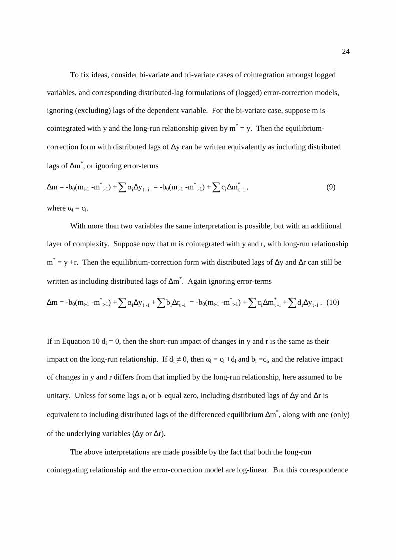
To fix ideas, consider bi-variate and tri-variate cases of cointegration amongst logged

variables, and corresponding distributed-lag formulations of (logged) error-correction models,

ignoring (excluding) lags of the dependent variable. For the bi-variate case, suppose m is

cointegrated with y and the long-run relationship given by m* = y. Then the equilibrium-

correction form with distributed lags of ∆y can be written equivalently as including distributed

lags of ∆m*, or ignoring error-terms

∆m = -b0(mt-1 -m*t-1) +∑ ∆ i-t i yα = -b0(mt-1 -m

*t-1) +∑ ∆ *

i-t i mc , (9)

where αi = ci.

With more than two variables the same interpretation is possible, but with an additional

layer of complexity. Suppose now that m is cointegrated with y and r, with long-run relationship

m* = y +r. Then the equilibrium-correction form with distributed lags of ∆y and ∆r can still be

written as including distributed lags of ∆m*. Again ignoring error-terms

∆m = -b0(mt-1 -m*t-1) +∑ ∆ i-t i yα +∑ ∆ i-t i rb = -b0(mt-1 -m

*t-1) +∑ ∆ *

i-t i mc +∑ ∆ i-ti yd . (10)

If in Equation 10 di = 0, then the short-run impact of changes in y and r is the same as their

impact on the long-run relationship. If di ≠ 0, then αi = ci +di and bi =ci, and the relative impact

of changes in y and r differs from that implied by the long-run relationship, here assumed to be

unitary. Unless for some lags αi or bi equal zero, including distributed lags of ∆y and ∆r is

equivalent to including distributed lags of the differenced equilibrium ∆m* , along with one (only)

of the underlying variables (∆y or ∆r).

The above interpretations are made possible by the fact that both the long-run

cointegrating relationship and the error-correction model are log-linear. But this correspondence

25

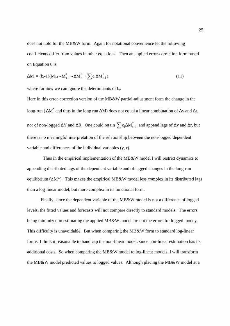
does not hold for the MB&W form. Again for notational convenience let the following

coefficients differ from values in other equations. Then an applied error-correction form based

on Equation 8 is

∆M t = (bt-1)(Mt-1 -*

1-tM - *tM∆ + *

i-ti Mc ∆∑ ) , (11)

where for now we can ignore the determinants of bt.

Here in this error-correction version of the MB&W partial-adjustment form the change in the

long-run ( *M∆ and thus in the long run ∆M) does not equal a linear combination of ∆y and ∆r,

nor of non-logged ∆Y and ∆R. One could retain *i-ti Mc ∆∑ , and append lags of ∆y and ∆r, but

there is no meaningful interpretation of the relationship between the non-logged dependent

variable and differences of the individual variables (y, r).

Thus in the empirical implementation of the MB&W model I will restrict dynamics to

appending distributed lags of the dependent variable and of lagged changes in the long-run

equilibrium (∆M*). This makes the empirical MB&W model less complex in its distributed lags

than a log-linear model, but more complex in its functional form.

Finally, since the dependent variable of the MB&W model is not a difference of logged

levels, the fitted values and forecasts will not compare directly to standard models. The errors

being minimized in estimating the applied MB&W model are not the errors for logged money.

This difficulty is unavoidable. But when comparing the MB&W form to standard log-linear

forms, I think it reasonable to handicap the non-linear model, since non-linear estimation has its

additional costs. So when comparing the MB&W model to log-linear models, I will transform

the MB&W model predicted values to logged values. Although placing the MB&W model at a

26

disadvantage, this seems preferable to comparing via a transformation of values from the log-

linear models.

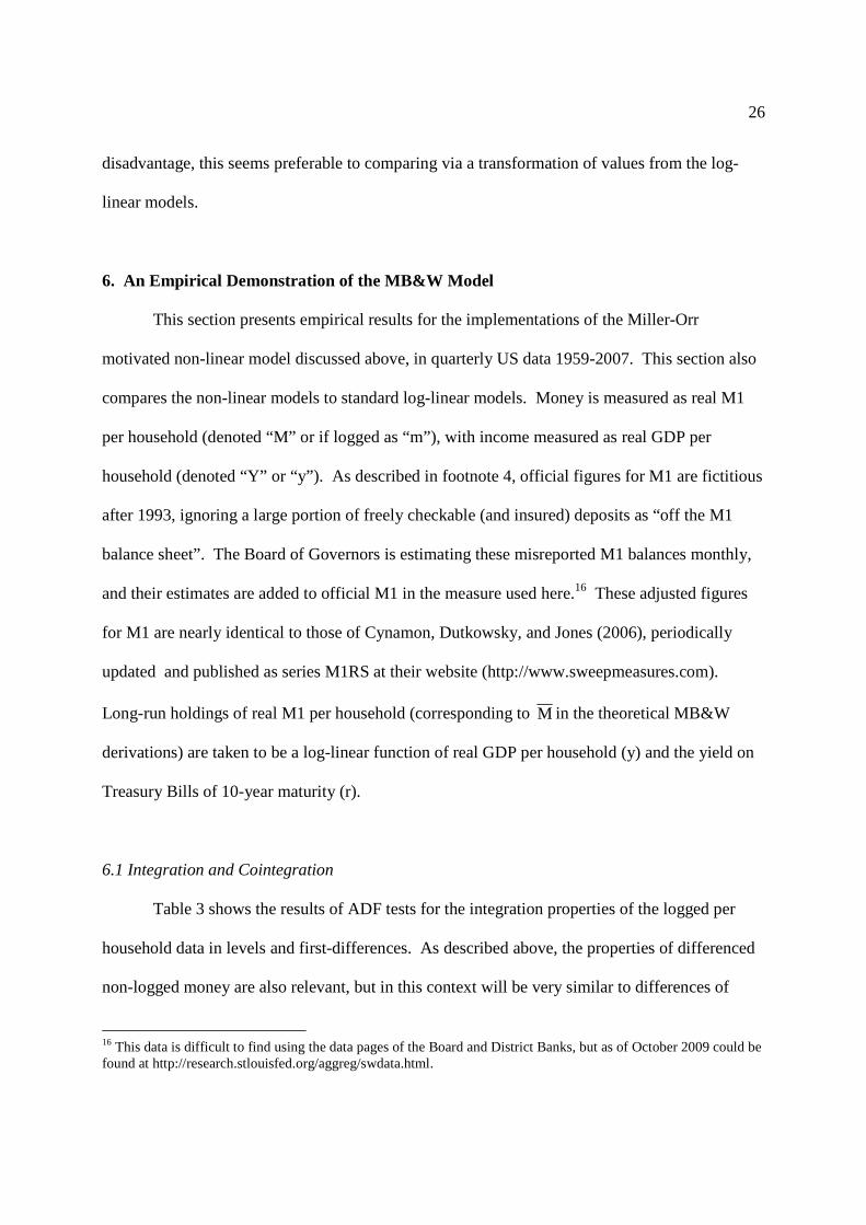
6. An Empirical Demonstration of the MB&W Model This section presents empirical results for the implementations of the Miller-Orr

motivated non-linear model discussed above, in quarterly US data 1959-2007. This section also

compares the non-linear models to standard log-linear models. Money is measured as real M1

per household (denoted “M” or if logged as “m”), with income measured as real GDP per

household (denoted “Y” or “y”). As described in footnote 4, official figures for M1 are fictitious

after 1993, ignoring a large portion of freely checkable (and insured) deposits as “off the M1

balance sheet”. The Board of Governors is estimating these misreported M1 balances monthly,

and their estimates are added to official M1 in the measure used here.16 These adjusted figures

for M1 are nearly identical to those of Cynamon, Dutkowsky, and Jones (2006), periodically

updated and published as series M1RS at their website (http://www.sweepmeasures.com).

Long-run holdings of real M1 per household (corresponding to M in the theoretical MB&W

derivations) are taken to be a log-linear function of real GDP per household (y) and the yield on

Treasury Bills of 10-year maturity (r).

6.1 Integration and Cointegration

Table 3 shows the results of ADF tests for the integration properties of the logged per

household data in levels and first-differences. As described above, the properties of differenced

non-logged money are also relevant, but in this context will be very similar to differences of

16 This data is difficult to find using the data pages of the Board and District Banks, but as of October 2009 could be found at http://research.stlouisfed.org/aggreg/swdata.html.

27

logged values. For each variable separate tests are conducted with and without a constant in the

test regression, and also with a constant and time trend, corresponding to three separate test

assumptions. In addition, test regression lags are selected via both the Schwarz and Akaike

criteria, for a total of six tests for the null of a unit root applied to each variable.

Rather than reporting all the individual tests, for each levels variable Table 3 reports the

minimum probability value across the tests. For the differenced data the maximum probability

value is reported. Thus the nominal p-value reported for the levels data is “cherry picked” in a

manner that leans towards rejection of a unit root (actual test size is greater than the reported p-

value), while the reported results for the differenced data are biased towards accepting the unit

root (actual test size is less than the reported p-value). Nonetheless a unit root is clearly accepted

for the variables in levels (with a lowest p-value of 0.25), while a unit root is rejected for the

differenced variables (with a largest p-value of 0.005). Although the use of aggregates scaled on

a per household basis is not standard practice, the results of Table 3 imply these variables have

the properties usually encountered in monetary and income aggregates.

Table 4 displays Johansen cointegration test results for the null of no cointegrating

relationships (versus more than zero) among logged real M1 per household, logged real GDP per

household, and the logged yield on Treasuries of 10-year maturity. Under the null the model is a

differenced VAR, so lag selection is done in this differenced VAR (no levels included), in which

case the AIC criteria selects two lags, while the SIC selects one lag. So results are displayed for

both one and two lags. Under both lag-selection criteria Table 4 shows that a null of no

cointegrating relationships is rejected, with (nominal) probability values of well under one-

percent. These variables are used in the Engle-Granger regression of the next paragraph.

28

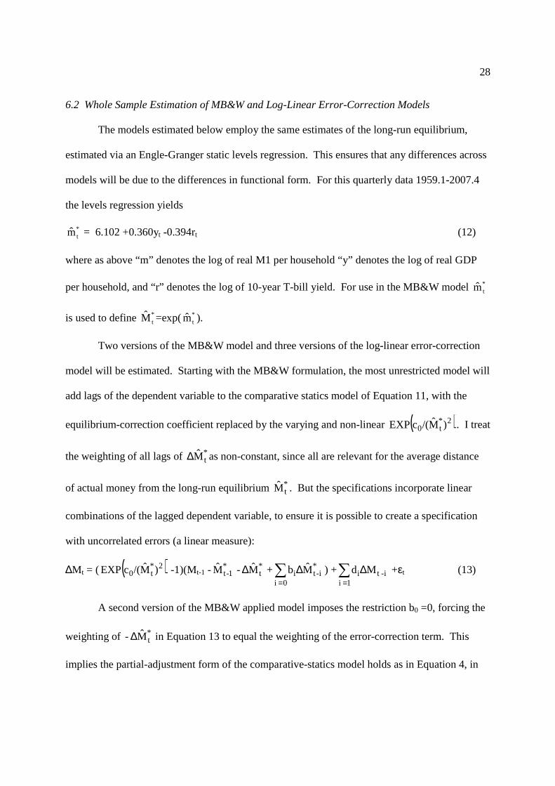
6.2 Whole Sample Estimation of MB&W and Log-Linear Error-Correction Models

The models estimated below employ the same estimates of the long-run equilibrium,

estimated via an Engle-Granger static levels regression. This ensures that any differences across

models will be due to the differences in functional form. For this quarterly data 1959.1-2007.4

the levels regression yields

*tm = 6.102 +0.360yt -0.394rt (12)

where as above “m” denotes the log of real M1 per household “y” denotes the log of real GDP

per household, and “r” denotes the log of 10-year T-bill yield. For use in the MB&W model *tm

is used to define *tM =exp( *

tm ).

Two versions of the MB&W model and three versions of the log-linear error-correction

model will be estimated. Starting with the MB&W formulation, the most unrestricted model will

add lags of the dependent variable to the comparative statics model of Equation 11, with the

equilibrium-correction coefficient replaced by the varying and non-linear ( )2*t0 )M/(cEXP . I treat

the weighting of all lags of *tM∆ as non-constant, since all are relevant for the average distance

of actual money from the long-run equilibrium *tM . But the specifications incorporate linear

combinations of the lagged dependent variable, to ensure it is possible to create a specification

with uncorrelated errors (a linear measure):

∆M t = ( ( )2*t0 )M/(cEXP -1)(Mt-1 -

*1-tM - *

tM∆ +∑=

∆0 i

*i-ti Mb ) +∑

=∆

1 ii-t i Md +εt (13)

A second version of the MB&W applied model imposes the restriction b0 =0, forcing the

weighting of *tM- ∆ in Equation 13 to equal the weighting of the error-correction term. This

implies the partial-adjustment form of the comparative-statics model holds as in Equation 4, in

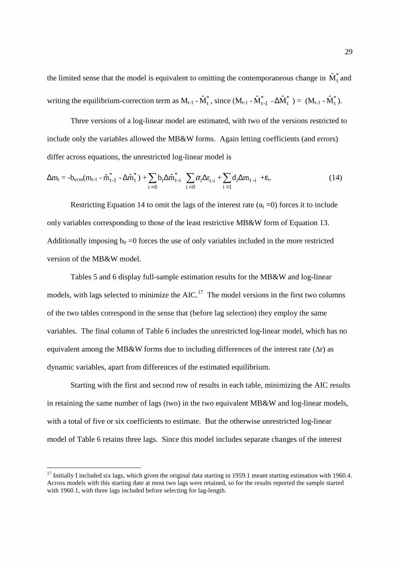
29

the limited sense that the model is equivalent to omitting the contemporaneous change in *tM and

writing the equilibrium-correction term as Mt-1 -*tM , since (Mt-1 -

*1-tM - *

tM∆ ) = (Mt-1 -*tM ).

Three versions of a log-linear model are estimated, with two of the versions restricted to

include only the variables allowed the MB&W forms. Again letting coefficients (and errors)

differ across equations, the unrestricted log-linear model is

∆mt = -becm(mt-1 -*

1-tm - *tm∆ ) +∑

=∆

0 i

*i-ti mb ∑

=∆

0 ii-ti rα +∑

=∆

1 ii-t i md +εt. (14)

Restricting Equation 14 to omit the lags of the interest rate (αi =0) forces it to include

only variables corresponding to those of the least restrictive MB&W form of Equation 13.

Additionally imposing b0 =0 forces the use of only variables included in the more restricted

version of the MB&W model.

Tables 5 and 6 display full-sample estimation results for the MB&W and log-linear

models, with lags selected to minimize the AIC.17 The model versions in the first two columns

of the two tables correspond in the sense that (before lag selection) they employ the same

variables. The final column of Table 6 includes the unrestricted log-linear model, which has no

equivalent among the MB&W forms due to including differences of the interest rate (∆r) as

dynamic variables, apart from differences of the estimated equilibrium.

Starting with the first and second row of results in each table, minimizing the AIC results

in retaining the same number of lags (two) in the two equivalent MB&W and log-linear models,

with a total of five or six coefficients to estimate. But the otherwise unrestricted log-linear

model of Table 6 retains three lags. Since this model includes separate changes of the interest

17 Initially I included six lags, which given the original data starting in 1959.1 meant starting estimation with 1960.4. Across models with this starting date at most two lags were retained, so for the results reported the sample started with 1960.1, with three lags included before selecting for lag-length.

30

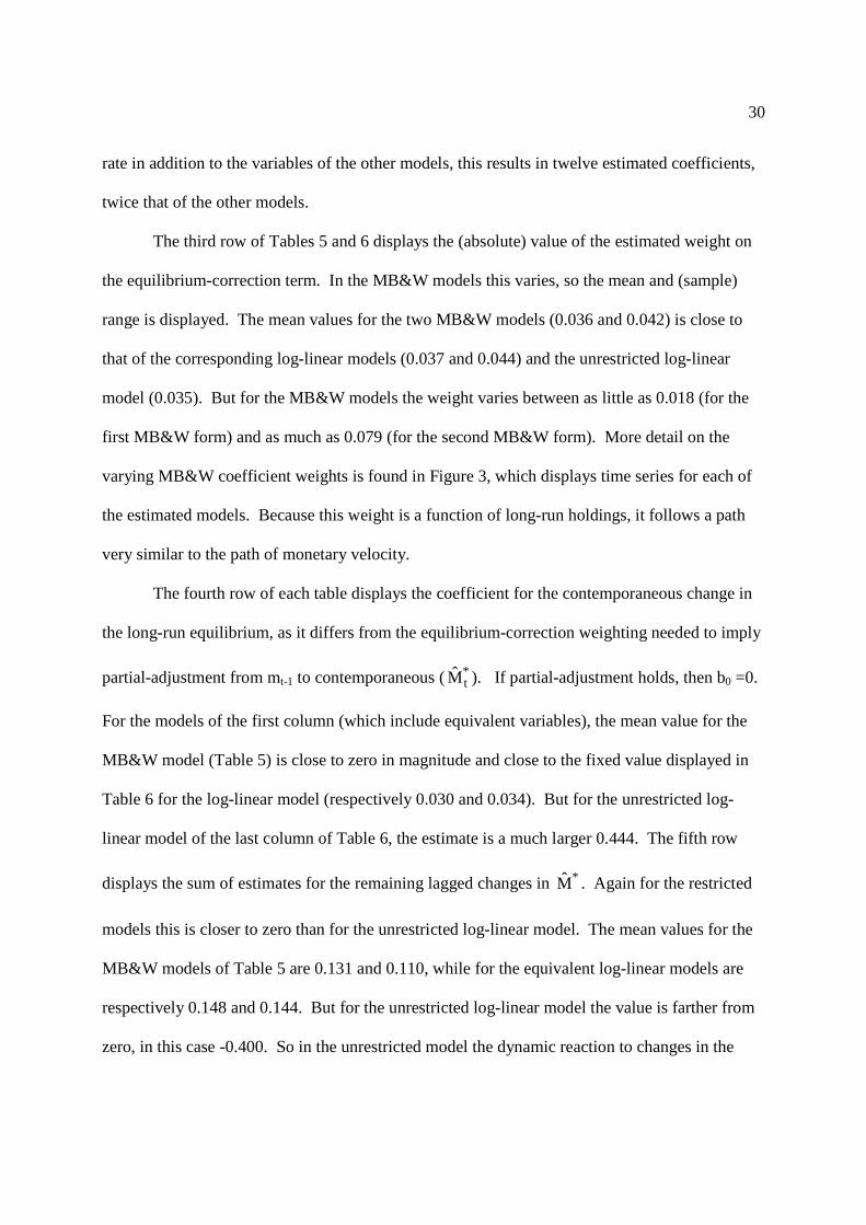
rate in addition to the variables of the other models, this results in twelve estimated coefficients,

twice that of the other models.

The third row of Tables 5 and 6 displays the (absolute) value of the estimated weight on

the equilibrium-correction term. In the MB&W models this varies, so the mean and (sample)

range is displayed. The mean values for the two MB&W models (0.036 and 0.042) is close to

that of the corresponding log-linear models (0.037 and 0.044) and the unrestricted log-linear

model (0.035). But for the MB&W models the weight varies between as little as 0.018 (for the

first MB&W form) and as much as 0.079 (for the second MB&W form). More detail on the

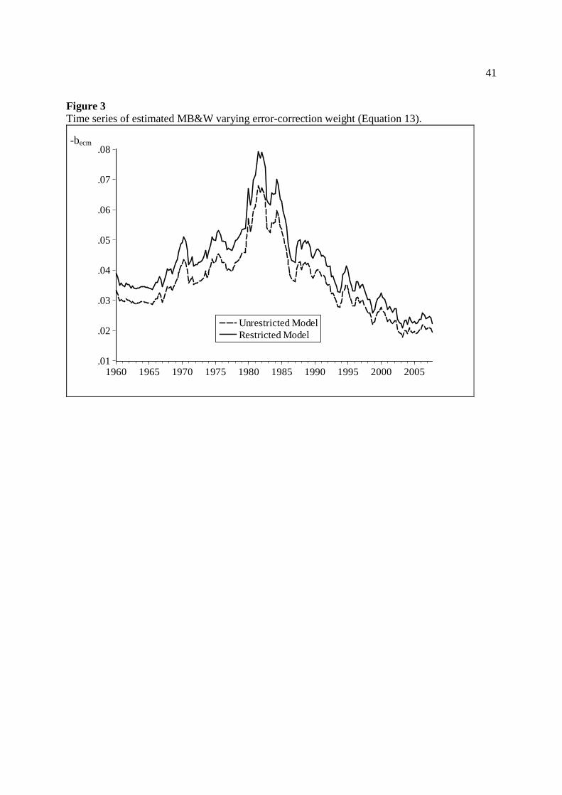
varying MB&W coefficient weights is found in Figure 3, which displays time series for each of

the estimated models. Because this weight is a function of long-run holdings, it follows a path

very similar to the path of monetary velocity.

The fourth row of each table displays the coefficient for the contemporaneous change in

the long-run equilibrium, as it differs from the equilibrium-correction weighting needed to imply

partial-adjustment from mt-1 to contemporaneous (*tM ). If partial-adjustment holds, then b0 =0.

For the models of the first column (which include equivalent variables), the mean value for the

MB&W model (Table 5) is close to zero in magnitude and close to the fixed value displayed in

Table 6 for the log-linear model (respectively 0.030 and 0.034). But for the unrestricted log-

linear model of the last column of Table 6, the estimate is a much larger 0.444. The fifth row

displays the sum of estimates for the remaining lagged changes in *M . Again for the restricted

models this is closer to zero than for the unrestricted log-linear model. The mean values for the

MB&W models of Table 5 are 0.131 and 0.110, while for the equivalent log-linear models are

respectively 0.148 and 0.144. But for the unrestricted log-linear model the value is farther from

zero, in this case -0.400. So in the unrestricted model the dynamic reaction to changes in the

31

long-run equilibrium is stronger and more complex than in the restricted models. As is about to

discussed, b0 =0 is rejected in the log-linear models but accepted in the MB&W model. So the

log-linear model selects for more complex dynamics than the MB&W model.

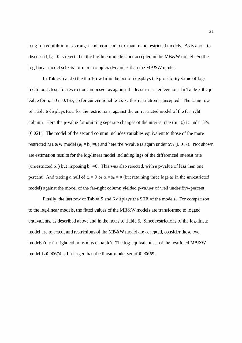
In Tables 5 and 6 the third-row from the bottom displays the probability value of log-

likelihoods tests for restrictions imposed, as against the least restricted version. In Table 5 the p-

value for b0 =0 is 0.167, so for conventional test size this restriction is accepted. The same row

of Table 6 displays tests for the restrictions, against the un-restricted model of the far right

column. Here the p-value for omitting separate changes of the interest rate (αi =0) is under 5%

(0.021). The model of the second column includes variables equivalent to those of the more

restricted MB&W model (αi = b0 =0) and here the p-value is again under 5% (0.017). Not shown

are estimation results for the log-linear model including lags of the differenced interest rate

(unrestricted αi ) but imposing b0 =0. This was also rejected, with a p-value of less than one

percent. And testing a null of αi = 0 or αi =b0 = 0 (but retaining three lags as in the unrestricted

model) against the model of the far-right column yielded p-values of well under five-percent.

Finally, the last row of Tables 5 and 6 displays the SER of the models. For comparison

to the log-linear models, the fitted values of the MB&W models are transformed to logged

equivalents, as described above and in the notes to Table 5. Since restrictions of the log-linear

model are rejected, and restrictions of the MB&W model are accepted, consider these two

models (the far right columns of each table). The log-equivalent ser of the restricted MB&W

model is 0.00674, a bit larger than the linear model ser of 0.00669.

32

6.3 Stability and Forecasting

In the simulation results, we found that linear and non-linear regression models of a

Miller-Orr world would have very similar fits within-sample. The difference between the

modeling approaches was found in stability and forecasting, particularly if the sample was

divided with respect to the level of long-run holdings (here *M ). Hence this section compares

stability and out-of-estimation-sample forecasting.

Although restrictions were rejected, I continue to show results for all the log-linear

models for two reasons. Not all nominal p-values were less than one-percent, and statistic

distributions are asymptotic, so there is room for differences of taste and judgment. And for

forecasting purposes simpler models are often preferred.18

Table 7 displays the results of stability tests when the sample is split with respect to

whether the estimated long-run *tM (of Equation 12) is greater or less than its median. Here I

display simple analysis-of-variance F-tests, and also likelihood-ratio tests which require adding

non-linear terms to each model, replacing each coefficient b with the term b*bD, where D is a (0,

1) dummy splitting the sample.

For simple F-tests, the p-values for both versions of the non-linear MB&W model are

well over ten-percent, 0.414 and 0.254 for both the unrestricted and restricted models of Table 5.

Results for the log-linear models depends upon tastes in test size. The first linear model (third

row) is most relevant, because the restrictions of the other log-linear models were rejected. For

this model the F-test p-value is 0.085, over five-percent but under ten percent.19

18 In this application it turns out that lags selected to minimize the more parsimonious sic results in models with larger forecast errors. 19 Recall that this model retains twelve variables, in contrast to the five or six variables of the other models (both linear and MB&W).

33

In Table 7 results of the likelihood-ratio tests are similar, except that p-values are closer

to zero. This does not matter for the non-linear MB&W models, where p-values are still well

over ten-percent (0.353 and 0.209) for the MB&W models of Table 5. But the p-value for the

unrestricted linear model is now 0.050. So stability is clearly accepted for the non-linear

MB&W model, but depending upon tastes could be rejected for the unrestricted log-linear

model.

Table 8 displays analogues of the simulation study of Table 2. Each model is estimated

over one half of the sample, with estimated coefficients used to generate forecast values for the

remaining sample.20 But as in Tables 2 and 7 the sample is split with respect to the level of long-

run demand ( *tM ), not time. Comparing forecast results to the results of re-estimation in the

forecast sample can be seen as a measure of the economic magnitude of any instability, although

in these small samples this is convoluted with estimation error.

The first two rows of Table 8 show results for the two versions of the MB&W model.

The forecast RMSE of the two are very similar, 82.11 for the least-restricted and 82.41 for the

more restricted version. Moving to the second column of results, when the MB&W models are

re-estimated over the forecast sub-sample, the standard errors of the models are 80.34 and 79.97,

again very close. More importantly, the difference between the forecast RMSE and the re-

estimation SER is only 2.2% and 3.1%. This is larger than the difference found in Table 2, but

of course estimation in Table 2 was over samples of 70,000 observations, and in a simulated

world of literal Miller-Orr structure.

The last three rows of Table 8 display the forecast and re-estimation results for the log-

linear models (of Table 6). Here the table starts with the least restricted model (as in the far

20 As in the simulation study the forecasts employ actual values of the lagged dependent variable.

34

right-hand column of Table 6), and then displays the results for the more restricted versions.

Again the forecast rmse’s are very similar, 0.006821, 0.006799 and 0.00636 as we go from least

to most restricted log-linear model. And among the log-linear models the forecast sample model

standard errors are similar. But again comparing forecast RMSE to the ser of the re-estimated

model, the differences are 19.9%, 15.5% and 16.8%. While not as large as in the simulated

Miller-Orr economy of Table 2 (where the difference was over 25%), this is still much greater

than for the MB&W models.

The final column of Table 8 allows comparison of the forecasts of the non-logged

MB&W models to the forecasts of the log-linear models. Transforming the forecasts and then

forecast errors of the MB&W models to log-equivalents, yields an RMSE of 0.005895 and

0.005877. Comparing to the RMSE of the log-linear models (from the first column) these are

about 15% smaller. Thus the statistical instability of the log-linear models is economically

relevant, in the sense that their ability to fit better within sample does not carry over to forecast

performance, especially when compared to the MB&W models designed for a Miller-Orr (S, s)

economy.

7. Conclusion

The recent applied literature provides empirical support across many countries and time

periods for non-linear smooth-adjustment models of money. It has been assumed that this

empirical evidence is consistent with monetary theory because the Miller-Orr model provides

economic motivation for standard smooth-adjustment empirics. But this paper shows the

intuitive arguments used in the smooth-adjustment literature are only partially correct. Most

critically, in a Miller-Orr economy a divergence of money holdings from long-run values does

35

not predict the probability or portion of accounts adjusting to target levels. Standard smooth-

adjustment models can improve on linear models when fitted to the aggregate data of a Miller-

Orr economy, but exhibit instabilities which undercut forecasting ability, particularly across

regimes with differing long-run demand.

The non-linear model theoretically implied by Miller-Orr behavior is found in the

Milbourne, Buckholtz and Wasan functional form. Although it can be described as a modified

smooth-adjustment model, it is of much simpler form than that of standard smooth-adjustment

models, with only one extra coefficient (beyond that of a linear model) to estimate. The

transition variable derived by MB&W is a static level, and it has not been understood that the

theory underlying the derivations of MB&W is essentially static, in contrast to the dynamic

language and transition variables used in the smooth-adjustment literature and in the language

used in MB&W’s own discussion. This paper has provided some heuristics for the support of

useful intuition and has used simulations to validate the MB&W derivations.

A unique characteristic of the Miller-Orr world is that the non-linearity which emerges in

the comparative-statics context involves a lagged dependent variable. This is due to aggregation

and the fact that in most monetary exchanges the net change in money held is zero. This aspect

of the Miller-Orr economy is unlikely to apply to other (S, s) contexts. But under aggregation it

was found that the variable subject to (S, s) management will differ from its average or long-run

value without implying that more agents than usual are close to making an adjustment. This

characteristic of the monetary Miller-Orr economy may apply in other non-monetary (S, s)

contexts such as menu-cost pricing models.

Taking the Miller-Orr world seriously implies an extensive agenda for applied modeling.

One implication is that models are distinguished in their stability and forecasting properties, not

36

by their within-sample fits. But the alternative to stable coefficients should be instability with

respect to the transition variable rather than instability with respect to time. Hence traditional

break-point stability tests neglect the important dimension. Empirical models inspired by a

Miller-Orr economy must control for population growth, using variables which come as closely

as possible to per-agent measures. For recent US data total households appears to be an adequate

scaling factor, but other contexts may require some ingenuity to find a useful scaling device.

And applied models inspired by the Miller-Orr (s, S) world will employ non-logged variables,

which interjects interesting issues of integration properties.

In a short empirical demonstration in US quarterly data, the MB&W static-transition

model performs as predicted by theoretical and simulation results. Unlike log-linear models it is

unambiguously stable. And the MB&W model forecasts with smaller RMSE than log-linear

models. Lag-selection criteria and tests of restrictions imply retention of many more variables in

the log-linear models. So despite its non-linear form the applied MB&W model is relatively

simple, employing half as many variables. It remains to be seen whether this holds for other

time periods and countries previously considered in the literature.

Acknowledgements

The author thanks Peter Ireland for extensive comments upon earlier drafts.

37

References

Bar-Ilan, A., 1990. Trigger-target rules need not be optimal with fixed adjustment costs: A simple comment on optimal money holding under uncertainty. International Economic Review 31 (1), 229-34

Bar-Ilan, A., Perry, D. and Stadje, W., 2004. A generalized impulse control model of cash

management. Journal of Economic Dynamics and Control 28, 1013-1033 Baumol, W. J., 1952. The transactions demand for cash- an inventory theoretic approach.

Quarterly Journal of Economics, 545-556 Bertola, G. and Caballero, R. J., 1990. Kinked adjustment costs and aggregate dynamics. NBER

Macroeconomics Annual, 237-88 Chen, S., and Wu, J., 2005. Long-run money demand revisited: Evidence from a non-linear

approach. Journal of International Money and Finance 24 (1), 19-37 Constantinides, G. and Richard, S. F., 1978. Existence of optimal simple policies for discounted-

cost inventory and cash management in continuous time. Operations Research 26 (4), 620-636 Corradi, V., and Swanson, N., 2006. The effect of data transformation on common cycle,

cointegration, and unit root tests: Monte Carlo results and a simple test. Journal of Econometrics 132, 195-229

Cynamon, B., Dutkowsky, D., and Jones, B., 2006. Redefining the monetary aggregates: A clean

sweep. Eastern Economic Journal 32 (4), 661-673 DeGroot, M., 1986. Probability and Statistics (Second Edition). Addison-Wesley, Boston, MA Greene, C. A., 2001. Trigger-target rules and the dynamics of aggregate money holdings. Journal

of Economic Dynamics and Control 15, 1193-1219 Harrison, J.M., Selke, T.M. and Taylor, T.M., 1983. Impulse control of Brownian motion.

Mathematics of Operations Research 8, 454-466 Haug, A. and Tam, J., 2007. A closer look at long-run U.S. money demand: Linear or nonlinear

error-correction with M0, M1, or M2? Economic Inquiry 45 (2), 363-376 Huang, C., Lin, C., and Cheng, J., 2001. Evidence on nonlinear error correction in money

demand: The case of Taiwan. Applied Economics 33 (13), 1727-36 Lee, C. and Chang, C., 2008. Long-run money demand in Taiwan revisited: Evidence from a

cointegrating STR approach. Applied Economics 40, 1061-1071

38

Lee, C., Chen, P. and Chang, C., 2007. Testing linearity in a cointegrating STR model for the money demand function: International evidence from G-7 countries. Mathematics and Computers in Simulation 76, 293-302

Milbourne, R. D., Buckholtz, P. and Wasan, M. T., 1983. A theoretical derivation of the

functional form of short run money holdings. Review of Economic Studies, 531-541 Miller, M.H. and Orr, D., 1966. A model of the demand for money by firms. Quarterly Journal of

Economics, 413-435 Ordonez, J., 2003. Stability and non-linear dynamics in the broad demand for money in Spain.

Economics Letters 78 (1), 139-46 Sarno, L., 1999. Adjustment costs and nonlinear dynamics in the demand for money: Italy, 1861-

1991. International Journal of Finance and Economics 4 (2), 155-77

Sarno, L., Taylor, M.P. and Peel, D.A., 2003. Nonlinear equilibrium correction in U.S. real money balances, 1869-1997. Journal of Money, Credit and Banking 35(5), 787-99

Tobin, J., 1956. The Interest elasticity of the transactions demand for cash. Review of Economics

and Statistics, 241-247 Vickson, R. G., 1985. Simple optimal policy for cash management: The average balance

requirement case. Journal of Financial & Quantitative Analysis 20(3), 353-369 Wu, J. and Hu, Y., 2007. Currency substitution and nonlinear error correction in Taiwan’s

demand for broad money. Applied Economics 39, 1635-1645

39

Figure 1 Probability distribution of (discrete) Miller-Orr holdings and empirical frequency of balances (m) with total M > M consistent with smooth-adjustment

0 E(m)Z HMean Empirical

40

Figure 2 Counter-example to smooth-adjustment intuition: Empirical frequency of balances (m) with total M > M

0 ZE(m) Mean Empirical

H

41

Figure 3 Time series of estimated MB&W varying error-correction weight (Equation 13).

.01

.02

.03

.04

.05

.06

.07

.08

1960 1965 1970 1975 1980 1985 1990 1995 2000 2005

Unrestricted ModelRestricted Model

-becm

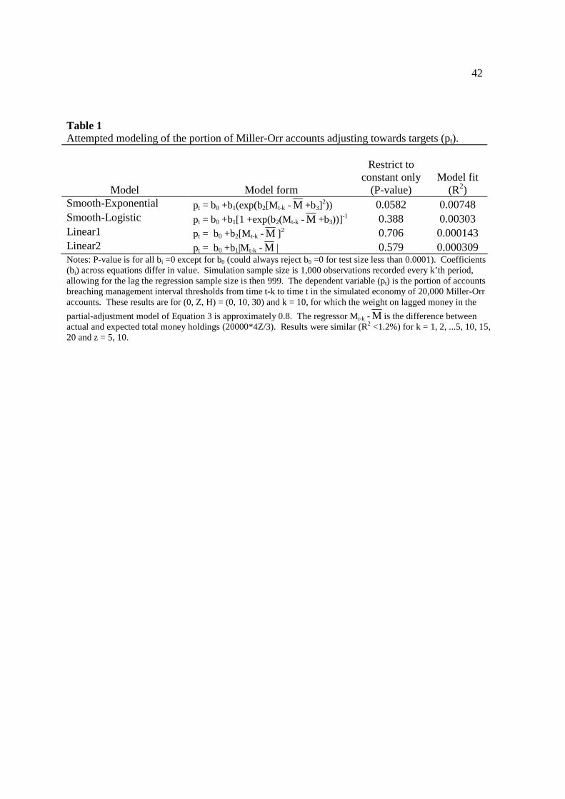
42

Table 1 Attempted modeling of the portion of Miller-Orr accounts adjusting towards targets (pt).

Model

Model form

Restrict to

constant only (P-value)

Model fit (R2)

Smooth-Exponential pt = b0 +b1(exp(b2[M t-k - M +b3]2)) 0.0582 0.00748

Smooth-Logistic pt = b0 +b1[1 +exp(b2(M t-k -M +b3))]-1 0.388 0.00303

Linear1 pt = b0 +b2[M t-k - M ]2 0.706 0.000143 Linear2 pt = b0 +b1|Mt-k - M | 0.579 0.000309 Notes: P-value is for all bi =0 except for b0 (could always reject b0 =0 for test size less than 0.0001). Coefficients (bi) across equations differ in value. Simulation sample size is 1,000 observations recorded every k’th period, allowing for the lag the regression sample size is then 999. The dependent variable (pt) is the portion of accounts breaching management interval thresholds from time t-k to time t in the simulated economy of 20,000 Miller-Orr accounts. These results are for (0, Z, H) = (0, 10, 30) and k = 10, for which the weight on lagged money in the

partial-adjustment model of Equation 3 is approximately 0.8. The regressor Mt-k - M is the difference between actual and expected total money holdings (20000*4Z/3). Results were similar (R2 <1.2%) for k = 1, 2, ...5, 10, 15, 20 and z = 5, 10.

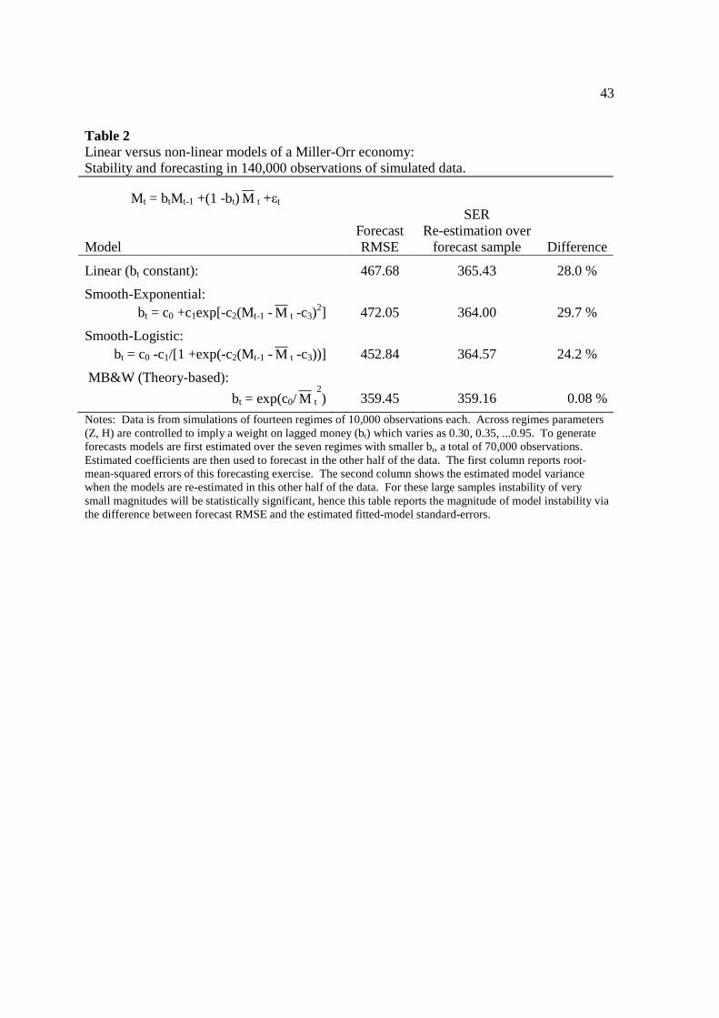
43

Table 2 Linear versus non-linear models of a Miller-Orr economy: Stability and forecasting in 140,000 observations of simulated data.

Mt = btMt-1 +(1 -bt) M t +εt

Model

Forecast RMSE

SER Re-estimation over

forecast sample

Difference

Linear (bt constant): 467.68 365.43 28.0 %

Smooth-Exponential: bt = c0 +c1exp[-c2(Mt-1 - M t -c3)

2]

472.05 364.00 29.7 %

Smooth-Logistic: bt = c0 -c1/[1 +exp(-c2(Mt-1 - M t -c3))]

452.84 364.57 24.2 %

MB&W (Theory-based):

bt = exp(c0/ M t2)

359.45 359.16 0.08 %

Notes: Data is from simulations of fourteen regimes of 10,000 observations each. Across regimes parameters (Z, H) are controlled to imply a weight on lagged money (bt) which varies as 0.30, 0.35, ...0.95. To generate forecasts models are first estimated over the seven regimes with smaller bt, a total of 70,000 observations. Estimated coefficients are then used to forecast in the other half of the data. The first column reports root-mean-squared errors of this forecasting exercise. The second column shows the estimated model variance when the models are re-estimated in this other half of the data. For these large samples instability of very small magnitudes will be statistically significant, hence this table reports the magnitude of model instability via the difference between forecast RMSE and the estimated fitted-model standard-errors.

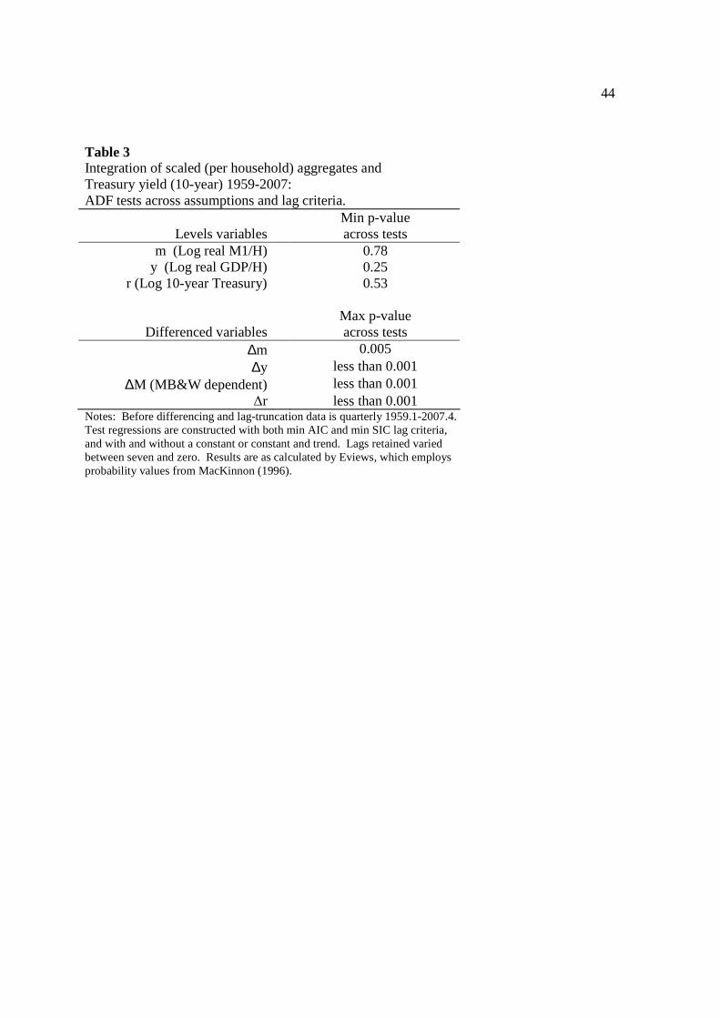
44

Table 3 Integration of scaled (per household) aggregates and Treasury yield (10-year) 1959-2007: ADF tests across assumptions and lag criteria.

Levels variables

Min p-value across tests

m (Log real M1/H) 0.78 y (Log real GDP/H) 0.25

r (Log 10-year Treasury) 0.53 Max p-value

Differenced variables across tests ∆m 0.005 ∆y less than 0.001

∆M (MB&W dependent) less than 0.001 ∆r less than 0.001

Notes: Before differencing and lag-truncation data is quarterly 1959.1-2007.4. Test regressions are constructed with both min AIC and min SIC lag criteria, and with and without a constant or constant and trend. Lags retained varied between seven and zero. Results are as calculated by Eviews, which employs probability values from MacKinnon (1996).

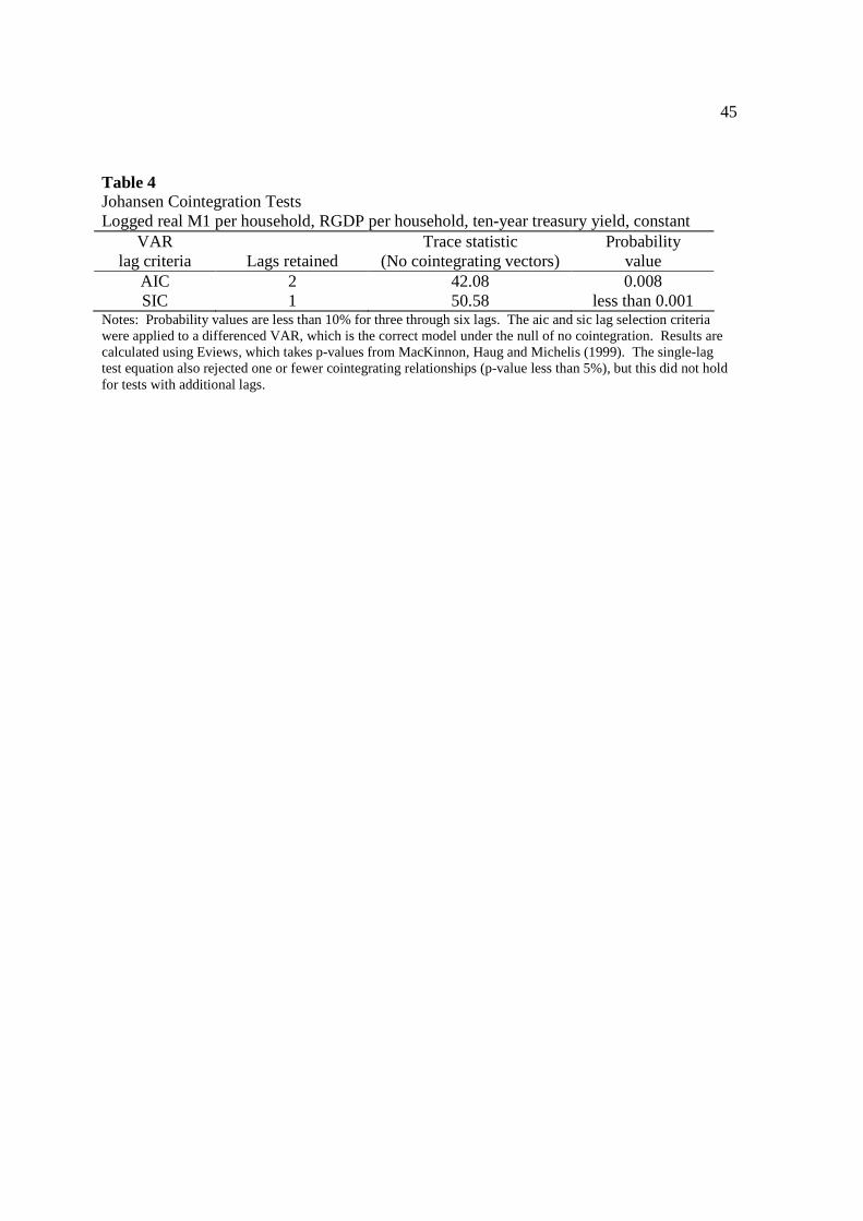
45

Table 4 Johansen Cointegration Tests Logged real M1 per household, RGDP per household, ten-year treasury yield, constant

VAR lag criteria

Lags retained

Trace statistic (No cointegrating vectors)

Probability value

AIC 2 42.08 0.008 SIC 1 50.58 less than 0.001

Notes: Probability values are less than 10% for three through six lags. The aic and sic lag selection criteria were applied to a differenced VAR, which is the correct model under the null of no cointegration. Results are calculated using Eviews, which takes p-values from MacKinnon, Haug and Michelis (1999). The single-lag test equation also rejected one or fewer cointegrating relationships (p-value less than 5%), but this did not hold for tests with additional lags.

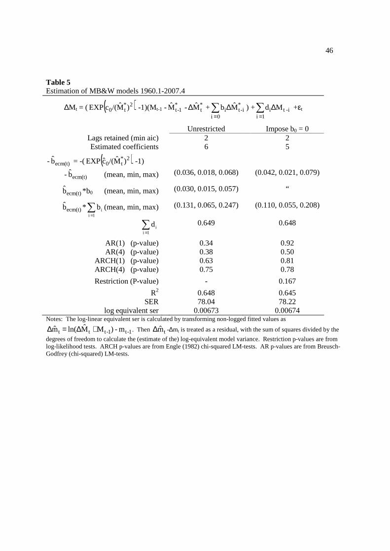
46

Table 5 Estimation of MB&W models 1960.1-2007.4

∆M t = ( ( )2*t0 )M/(cEXP -1)(Mt-1 -

*1-tM - *

tM∆ +∑=

∆0 i

*i-ti Mb ) +∑

=∆

1 ii-t i Md +εt

Unrestricted Impose b0 = 0 Lags retained (min aic) 2 2 Estimated coefficients 6 5

ecm(t)b- = -( ( )2*t0 )M/(cEXP -1)

ecm(t)b- (mean, min, max) (0.036, 0.018, 0.068) (0.042, 0.021, 0.079)

ecm(t)b *b0 (mean, min, max) (0.030, 0.015, 0.057) “

ecm(t)b *∑=1 i

ib (mean, min, max) (0.131, 0.065, 0.247) (0.110, 0.055, 0.208)

∑=1 i

id 0.649 0.648

AR(1) (p-value) 0.34 0.92 AR(4) (p-value) 0.38 0.50

ARCH(1) (p-value) 0.63 0.81 ARCH(4) (p-value) 0.75 0.78

Restriction (P-value) - 0.167

R2 0.648 0.645 SER 78.04 78.22

log equivalent ser 0.00673 0.00674 Notes: The log-linear equivalent ser is calculated by transforming non-logged fitted values as

1-t1-ttt m- )M Mln( m +∆=∆ . Then tm∆ -∆mt is treated as a residual, with the sum of squares divided by the

degrees of freedom to calculate the (estimate of the) log-equivalent model variance. Restriction p-values are from log-likelihood tests. ARCH p-values are from Engle (1982) chi-squared LM-tests. AR p-values are from Breusch-Godfrey (chi-squared) LM-tests.

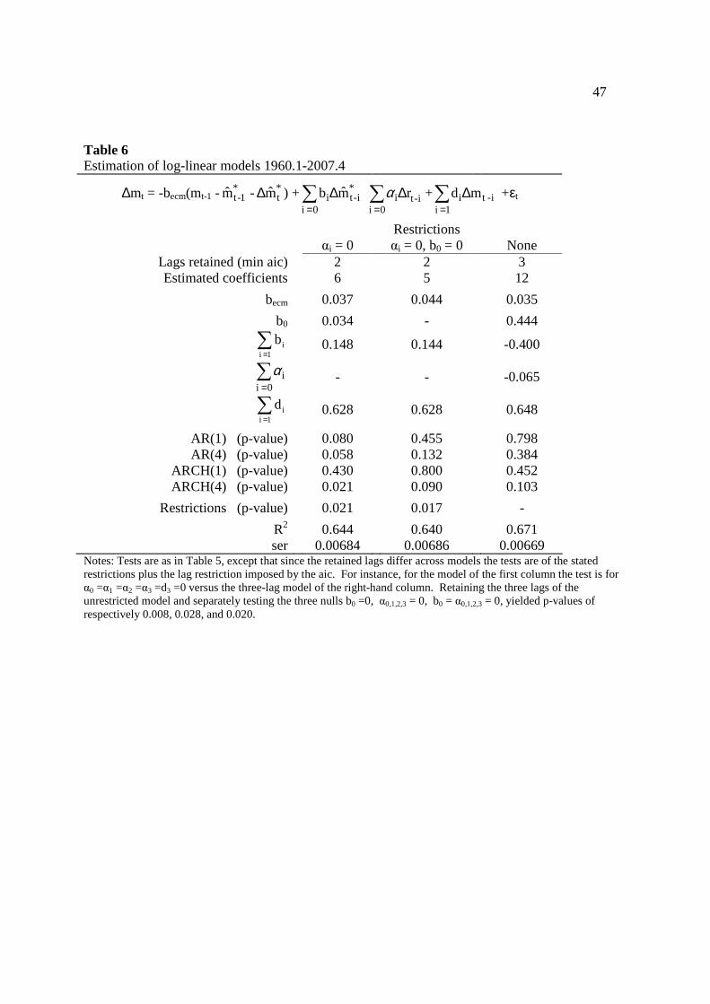
47

Table 6 Estimation of log-linear models 1960.1-2007.4

∆mt = -becm(mt-1 -*

1-tm - *tm∆ ) +∑

=∆

0 i

*i-ti mb ∑

=∆

0 ii-ti rα +∑

=∆

1 ii-t i md +εt

Restrictions αi = 0 αi = 0, b0 = 0 None

Lags retained (min aic) 2 2 3 Estimated coefficients 6 5 12

becm 0.037 0.044 0.035

b0 0.034 - 0.444

∑=1 i

ib 0.148 0.144 -0.400

∑=0 i

iα -

-

-0.065

∑=1 i

id 0.628 0.628 0.648

AR(1) (p-value) 0.080 0.455 0.798 AR(4) (p-value) 0.058 0.132 0.384

ARCH(1) (p-value) 0.430 0.800 0.452 ARCH(4) (p-value) 0.021 0.090 0.103

Restrictions (p-value) 0.021 0.017 -

R2 0.644 0.640 0.671 ser 0.00684 0.00686 0.00669

Notes: Tests are as in Table 5, except that since the retained lags differ across models the tests are of the stated restrictions plus the lag restriction imposed by the aic. For instance, for the model of the first column the test is for α0 =α1 =α2 =α3 =d3 =0 versus the three-lag model of the right-hand column. Retaining the three lags of the unrestricted model and separately testing the three nulls b0 =0, α0,1,2,3 = 0, b0 = α0,1,2,3 = 0, yielded p-values of respectively 0.008, 0.028, and 0.020.

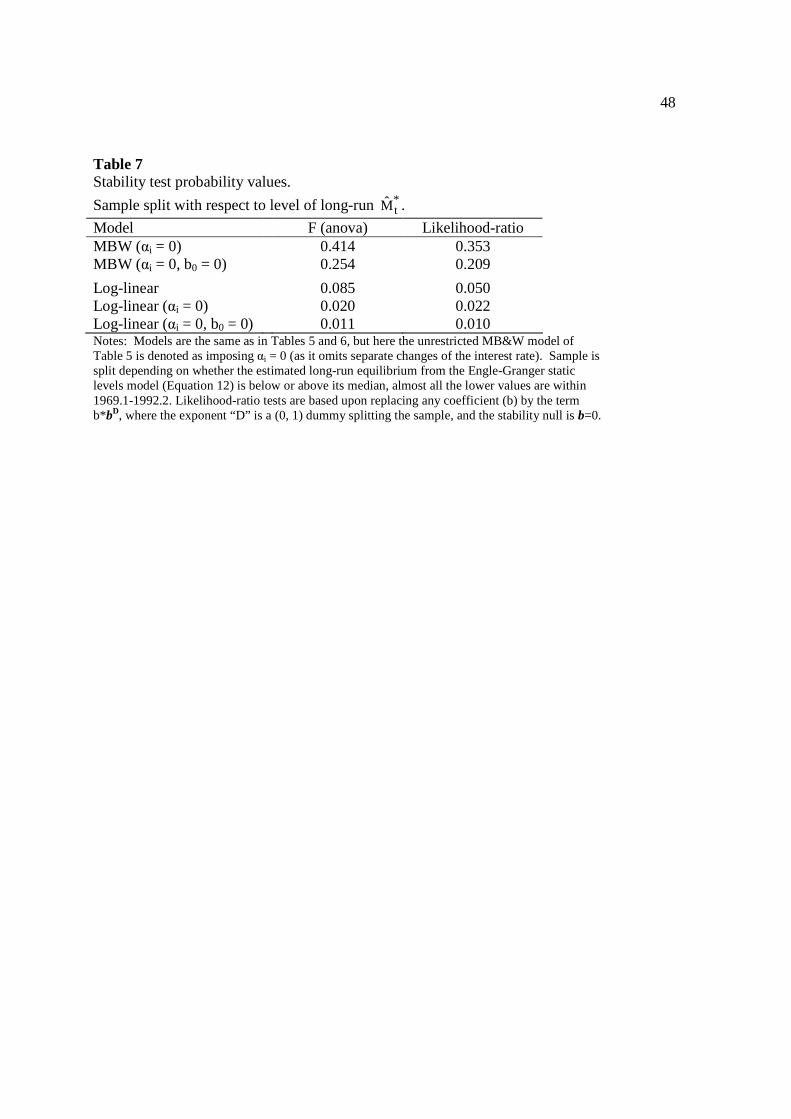
48

Table 7 Stability test probability values.

Sample split with respect to level of long-run *tM .

Model F (anova) Likelihood-ratio MBW (αi = 0) 0.414 0.353 MBW (αi = 0, b0 = 0) 0.254 0.209

Log-linear 0.085 0.050 Log-linear (αi = 0) 0.020 0.022 Log-linear (αi = 0, b0 = 0) 0.011 0.010 Notes: Models are the same as in Tables 5 and 6, but here the unrestricted MB&W model of Table 5 is denoted as imposing αi = 0 (as it omits separate changes of the interest rate). Sample is split depending on whether the estimated long-run equilibrium from the Engle-Granger static levels model (Equation 12) is below or above its median, almost all the lower values are within 1969.1-1992.2. Likelihood-ratio tests are based upon replacing any coefficient (b) by the term b*bD, where the exponent “D” is a (0, 1) dummy splitting the sample, and the stability null is b=0.

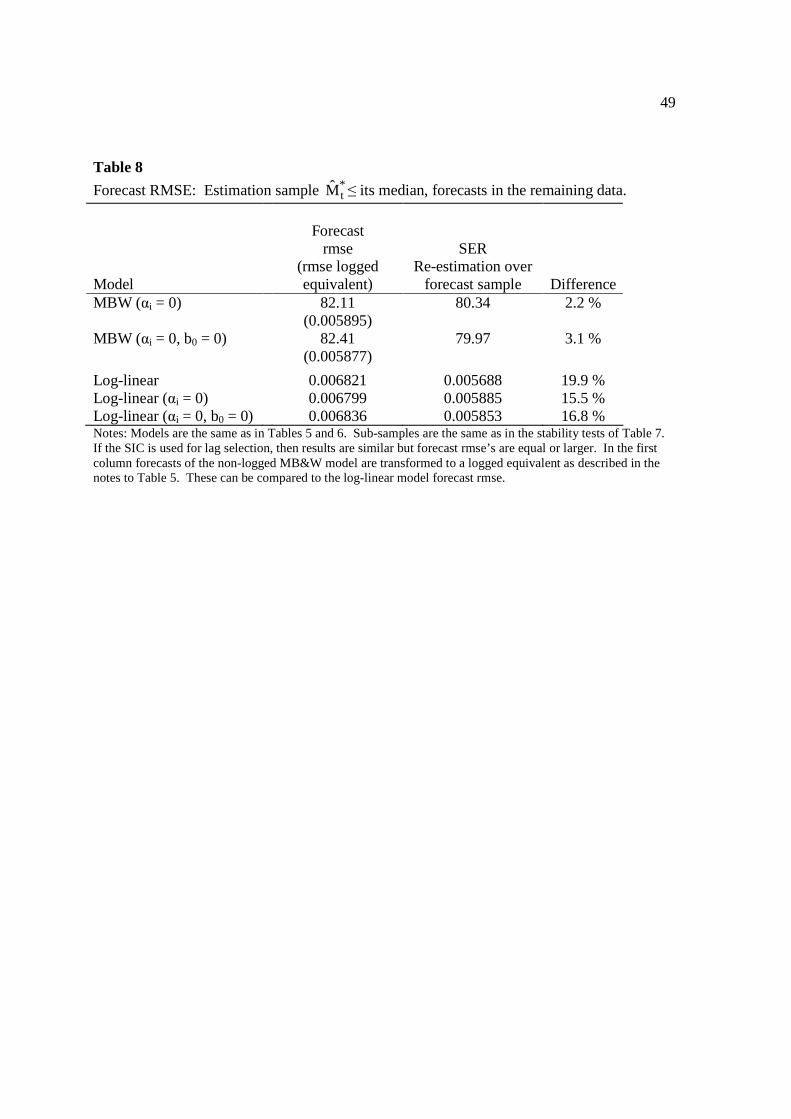
49

Table 8

Forecast RMSE: Estimation sample *tM ≤ its median, forecasts in the remaining data.

Model

Forecast

rmse (rmse logged equivalent)

SER Re-estimation over

forecast sample

Difference MBW (αi = 0) 82.11

(0.005895) 80.34 2.2 %

MBW (αi = 0, b0 = 0) 82.41 (0.005877)

79.97 3.1 %

Log-linear 0.006821 0.005688 19.9 % Log-linear (αi = 0) 0.006799 0.005885 15.5 % Log-linear (αi = 0, b0 = 0) 0.006836 0.005853 16.8 % Notes: Models are the same as in Tables 5 and 6. Sub-samples are the same as in the stability tests of Table 7. If the SIC is used for lag selection, then results are similar but forecast rmse’s are equal or larger. In the first column forecasts of the non-logged MB&W model are transformed to a logged equivalent as described in the notes to Table 5. These can be compared to the log-linear model forecast rmse.