SMGSPC Service Troubleshooting Steps - ECD
145
SuperM.O.L.E. for WINDOWS Software User’s guide for SuperM.O.L.E. Thinline and SuperM.O.L.E. GOLD SuperM.O.L.E. for Windows A37-0909-32 Rev 2.3
Transcript of SMGSPC Service Troubleshooting Steps - ECD

SuperM.O.L.E. for WINDOWS
Software User’s guide forSuperM.O.L.E. Thinline and SuperM.O.L.E. GOLD
SuperM.O.L.E. for WindowsA37-0909-32 Rev 2.3

SINCE 1964
ECD, Inc.4287-A S.E. International WayMilwaukie, Oregon 97222-8825
Telephone: (800) 323-4548(503) 659-6100
FAX: (503) 659-4422Technical Support: (800) 323-4548
Email: [email protected]: http://www.ecd.com

ECD, INC.End User License Agreementfor ECD Software Products
NOTICE TO USER:THIS IS A CONTRACT. BY INSTALLING THIS SOFTWARE YOUACCEPT ALL THE TERMS AND CONDITIONS OF THIS AGREEMENT.
This Electronic Controls Design, Incorporated ("ECD") End User LicenseAgreement accompanies ECD software products and related explanatorymaterials ("Software"). The term “Software” also shall include anyupgrades, modified versions or updates of the Software licensed to you byECD. Please read the Agreement on the following page carefully. At theend, you will be asked to accept this agreement and continue to install or,if you do not wish to accept this Agreement, to decline this agreement, inwhich case you will not be able to use the Software.

Upon your acceptance of this Agreement, ECD grants to you a nonexclusive license to use theSoftware, provided that you agree to the following:1. Use of the Software.
You may install the Software on a hard disk or other storage device; install and use the Software on a file serverfor use on a network for the purposes of (i) permanent installation onto hard disks or other storage devices or(ii) use of the Software over such network; and make backup copies of the Software.
ECD Software is sold for use with one or more ECD hardware product: M.O.L.E.®, SuperM.O.L.E.® Thinline,SuperM.O.L.E.® Gold, SuperM.O.L.E.® Gold RF, AeroM.O.L.E.®, WaveRIDER®, OvenRIDER™, INDATA® orCureTRAK™. This Agreement allows you to use the Software with the ECD hardware product purchased. Youmust order and pay for additional copies of the software if additional ECD hardware products are purchased.
You may make and distribute unlimited copies of the Software, licensed with the respective ECD hardwareproduct you purchased, as long as each copy that you make and distribute contains this Agreement, the samecopyright and other proprietary notices pertaining to this Software that appear in the Software, and that thepurpose of distributing the software is for the purpose of viewing, analyzing and reporting data captured by theassociated ECD hardware product. If you download an updated version of the Software, for the respectivehardware product you purchased, from the Internet or similar on-line source, you must include the ECDcopyright notice for the Software with any on-line distribution and on any media you distribute that includes theSoftware.
2. Copyright and Trademark RightsThe Software is owned by ECD and its suppliers, and its structure, organization and code are valuable tradesecrets of ECD and its suppliers. The Software also is protected by United States Copyright Law andInternational Treaty provisions. You may use trademarks only insofar as required to comply with Section 1 ofthis Agreement and to identify printed output produced by the Software, in accordance with accepted trademarkpractice, including identification of trademark owner’s name. Such use of any trademark does not give you anyrights of ownership in that trademark. Except as stated above, this Agreement does not grant you anyintellectual property rights in the Software.
3. RestrictionsYou agree not to modify, adapt, translate, reverse engineer, decompile, disassemble or otherwise attempt todiscover the source code of the Software. The Software is licensed and distributed by ECD for viewing,analyzing and reporting data captured by associated ECD hardware products.
4. No WarrantyThe Software is being delivered to you AS IS and ECD makes no warranty as to its use or performance. ECDAND ITS SUPPLIERS DO NOT AND CANNOT WARRANT THE PERFORMANCE OR RESULTS YOU MAYOBTAIN BY USING THE SOFTWARE OR DOCUMENTATION. ECD AND ITS SUPPLIERS MAKE NOWARRANTIES, EXPRESS OR IMPLIED, AS TO NONINFRINGEMENT OF THIRD PARTY RIGHTS,MERCHANTABILITY, OR FITNESS FOR ANY PARTICULAR PURPOSE. IN NO EVENT WILL ECD OR ITSSUPPLIERS BE LIABLE TO YOU FOR ANY CONSEQUENTIAL, INCIDENTAL OR SPECIAL DAMAGES,INCLUDING ANY LOST PROFITS OR LOST SAVINGS, EVEN IF AN ECD REPRESENTATIVE HAS BEENADVISED OF THE POSSIBILITY OF SUCH DAMAGES, OR FOR ANY CLAIM BY ANY THIRD PARTY. Somestates or jurisdictions do not allow the exclusion or limitation of incidental, consequential or special damages, orthe exclusion of implied warranties or limitations on how long an implied warranty may last, so the abovelimitations may not apply to you.
5. Governing Law and General ProvisionsThis Agreement will be governed by the laws of the State of Oregon, U.S.A., excluding the application of itsconflicts of law rules. This Agreement will not be governed by the United Nations Convention on Contracts forthe International Sale of Goods, the application of which is expressly excluded. If any part of this Agreement isfound void and unenforceable, it will not affect the validity of the balance of the Agreement, which shall remainvalid and enforceable according to its terms. You agree that the Software will not be shipped, transferred orexported into any country or used in any manner prohibited by the United States Export Administration Act orany other export laws, restrictions or regulations. This Agreement shall automatically terminate upon failure byyou to comply with its terms. This Agreement may only be modified in writing signed by an authorized officer ofECD.
Unpublished-rights reserved under the copyright laws of the United States.Electronic Controls Design Incorporated, 4287-A SE International Way, Milwaukie, Oregon 97222 USA.
YOUR ACCEPTANCE OF THE FOREGOING AGREEMENT WAS INDICATED DURING INSTALLATION.

SuperM.O.L.E. for Windows ♦♦♦♦ i♦♦♦♦
Table of Contents
INTRODUCTION .......................................................................................vi
! How to Use This Manual.............................................................................................. vi! Terms Used in this Manual .......................................................................................... vi! Fonts Used in this Manual ........................................................................................... vi
PC Hardware Requirements...................................................................vii
Software Installation..............................................................................viii
! Installing SMFW on a PC with Windows 3.X ..............................................................viii! Installing SMFW on a PC with Windows 95, 98 or NT................................................. ix! Starting the Software .................................................................................................... x
1.0 A Look at SMFW..................................................................................1
1.1 SMFW Workbook Features.......................................................................................11.2 Standard Worksheet functions ..................................................................................3
1.2.1 Worksheet tabs................................................................................................31.2.2 Selecting Worksheets......................................................................................31.2.3 Split-bar ...........................................................................................................31.2.4 Worksheet Tab Scroll Arrows ..........................................................................31.2.5 Scrollbars.........................................................................................................4

♦♦♦♦ ii♦♦♦♦ SuperM.O.L.E. for Windows
2.0 Worksheet Descriptions .....................................................................5
2.1 The Welcome Worksheet..........................................................................................52.1.1 Welcome Worksheet Menus and Toolbar .......................................................62.1.2 Company/Report Name ...................................................................................7
2.2 Finder Worksheet ......................................................................................................82.2.1 Finder Menus and Toolbar...............................................................................92.2.2 Parameter Groups .........................................................................................102.2.3 Parameter Labels ..........................................................................................112.2.4 Parameter Units.............................................................................................112.2.5 Data Run Rows..............................................................................................122.2.6 Selected Run .................................................................................................122.2.7 Filters .............................................................................................................13
2.3 Profile Worksheet ....................................................................................................152.3.1 Profile Menus and Toolbar.............................................................................162.3.2 M.O.L.E. Status .............................................................................................172.3.3 Tool Status Box .............................................................................................182.3.4 Magnify Map ..................................................................................................182.3.5 The Data Table..............................................................................................192.3.6 Sensor Locations ...........................................................................................192.3.7 Channel Check Boxes ...................................................................................192.3.8 Status Bar......................................................................................................202.3.9 Data Tabs ......................................................................................................21
2.3.9.1 Value .................................................................................................212.3.9.2 Time to Reference.............................................................................222.3.9.3 T Above Ref ......................................................................................222.3.9.4 Statistics ............................................................................................242.3.9.5 Zone Slopes ......................................................................................242.3.9.6 Summary Statistics............................................................................24
2.3.10 The Data Graph...........................................................................................252.3.10.1 X and Y-Axes and Labels ................................................................262.3.10.2 Autoscaling......................................................................................262.3.10.3 Data Plots........................................................................................272.3.10.4 Process Origin.................................................................................282.3.10.5 X-Cursors ........................................................................................292.3.10.6 X-axis Units .....................................................................................312.3.10.7 Temperature Reference Lines.........................................................312.3.10.8 Zones and Zone Sizes ....................................................................322.3.10.9 Zone Temperatures.........................................................................322.3.10.10 Zone Matrix ...................................................................................33

SuperM.O.L.E. for Windows ♦♦♦♦ iii♦♦♦♦
3.0 Menu and Tool Commands ..............................................................34
3.1 File Menu.................................................................................................................343.1.1 New................................................................................................................343.1.2 Open..............................................................................................................353.1.3 Close..............................................................................................................353.1.4 Import ............................................................................................................363.1.5 Save...............................................................................................................373.1.6 Save As .........................................................................................................373.1.7 Save As Text .................................................................................................383.1.8 Save as Text Archive.....................................................................................383.1.9 Load Text Archive..........................................................................................393.1.10 Tag File Number ..........................................................................................403.1.11 Configuration ...............................................................................................413.1.12 List-Print Data ..............................................................................................423.1.13 Page Setup..................................................................................................433.1.14 Print Options ................................................................................................443.1.15 Page Header / Footer ..................................................................................453.1.16 Print Preview................................................................................................463.1.17 Print .............................................................................................................473.1.18 Report Setup................................................................................................483.1.19 File Viewer ...................................................................................................493.1.20 Print Report..................................................................................................513.1.21 Recent Files 1, 2, 3, etc... ............................................................................513.1.22 Exit...............................................................................................................513.1.23 Language.....................................................................................................51
3.2 Edit Menu ................................................................................................................523.2.1 Undo ..............................................................................................................523.2.2 Redo ..............................................................................................................523.2.3 Remove Row .................................................................................................523.2.4 Hide Row .......................................................................................................52
3.3 View Menu...............................................................................................................533.3.1 Toolbar ..........................................................................................................533.3.2 Status Bar......................................................................................................533.3.3 Zoom In .........................................................................................................533.3.4 Zoom Out.......................................................................................................533.3.5 100% .............................................................................................................54
3.4 Format Menu ...........................................................................................................553.4.1 Bold ...............................................................................................................553.4.2 Italic ...............................................................................................................553.4.3 Underline .......................................................................................................553.4.4 Alignment (Left, Center, Right) ......................................................................55

♦♦♦♦ iv♦♦♦♦ SuperM.O.L.E. for Windows
3.5 Profile Menu ............................................................................................................563.5.1 Part ................................................................................................................563.5.2 Process..........................................................................................................573.5.3 Sensors..........................................................................................................583.5.4 Channel Lag ..................................................................................................613.5.5 Units...............................................................................................................633.5.6 Scaling...........................................................................................................643.5.7 Temp Ref Lines (Temperature Reference Lines) ..........................................653.5.8 Oven Configure..............................................................................................66
• Zone Configuration .....................................................................................67• Temperatures .............................................................................................69• Conveyor speed..........................................................................................70• Oven Models...............................................................................................71
3.5.9 Zone Matrix....................................................................................................743.5.10 Calculate h-Factor .......................................................................................743.5.11 Profile Defaults Sub-Menu...........................................................................75
3.6 M.O.L.E. Menu ........................................................................................................763.6.1 Set M.O.L.E. Clock ........................................................................................763.6.2 M.O.L.E. Configure ........................................................................................783.6.3 RF M.O.L.E. Data ..........................................................................................803.6.4 Read M.O.L.E. Data ......................................................................................843.6.5 M.O.L.E. Defaults Sub-Menu.........................................................................85
3.6.5.1 RF Alarm Points ................................................................................863.7 Tools Menu..............................................................................................................88
3.7.1 Magnify Tool ..................................................................................................883.7.2 Slope Tool .....................................................................................................903.7.3 Peak Difference Tool .....................................................................................923.7.4 Overlay Tool ..................................................................................................933.7.5 Total Heat Tool ..............................................................................................953.7.6 3-D Tool .........................................................................................................973.7.7 Measure Tool.................................................................................................993.7.8 Notes Tool ...................................................................................................1013.7.9 Prediction Tool.............................................................................................1023.7.10 Tolerance Band Tool .................................................................................1083.7.11 Erase Object(s)..........................................................................................1113.7.12 Erase All ....................................................................................................111
3.8 Window Menu........................................................................................................1123.8.1 Cascade.......................................................................................................1123.8.2 Tile...............................................................................................................1133.8.3 Open File .....................................................................................................113

SuperM.O.L.E. for Windows ♦♦♦♦ v♦♦♦♦
3.9 Navigate Menu ......................................................................................................1143.10 Help Menu ...........................................................................................................115
3.10.1 Index..........................................................................................................1153.10.2 Using Help .................................................................................................1163.10.3 About M.O.L.E. ..........................................................................................1173.10.4 Context Help ..............................................................................................1173.10.5 Copy Button ...............................................................................................117
4.0 SMFW Sensor Information .............................................................118
4.1 Configuring Sensors ..............................................................................................1184.2 Using SMFW with the AeroM.O.L.E. Profiler.........................................................1204.3 Using SMFW with the UV Sensor..........................................................................121
Appendix A: Parameter Definitions .....................................................122
Appendix B: Pull Down Menus & Toolbar Buttons.............................128

♦♦♦♦ vi♦♦♦♦ SuperM.O.L.E. for Windows
INTRODUCTION
!!!! How to Use This Manual
This Software User’s Guide explains how to use ECD’s (Electronic Controls DesignInc.) SuperM.O.L.E. for Windows software.
This manual is written for users of varied experience. If a section covers information youalready know, feel free to skip to the next section.
• You do not need to be a computer expert to use this manual or SuperM.O.L.E. forWindows software.
• The manual assumes you are familiar with Microsoft Windows.
!!!! Terms Used in this Manual
ECD Inc. introduced the original M.O.L.E. (Multichannel Occurrent Logger Evaluator) in1986. ECD currently produces several models of the M.O.L.E. for use in a wide varietyof applications. In this manual, we will use M.O.L.E. to refer to the SuperM.O.L.E.Thinline, and the SuperM.O.L.E. GOLD data recording devices. The followingstatements describe special terms that will be used in this manual.
• SuperM.O.L.E. for Windows software will be referred to as SMFW.
• Workbook, contains all of the worksheets and the uploaded data set saved with fileextension (.MSM).
• Worksheet, the individual pages or sheets in the workbook file.
• Data Set, multiple data runs uploaded into the workbook file.
• Data Run / Experiment, the data uploaded from the M.O.L.E..
• Thermocouple, may be referred to as T/C.
• Informs the user that the note includes important information.
• Informs the user that the note includes a handy software tip.
!!!! Fonts Used in this Manual
This manual uses a special font to indicate terms or words that can be found directly onthe PC display.
For Example: Select the Open command from the File menu to open a new workbookfile. This font indicates the words Open and File are actually found in the PC display.

SuperM.O.L.E. for Windows ♦♦♦♦ vii♦♦♦♦
PC Hardware Requirements
Before SuperM.O.L.E. for Windows can be used, a 486 or better computer that can runWindows will be required to run the software. Specific recommendations are as follows:
CPU, RAM, Hardware: Pentium processor16 megabytes of RAM (minimum).24 megabytes of free disk space.
Operating System: Windows 3.1, Windows for Workgroups 3.11, Windows 95, 98 or Windows NT.
For optimum performance when running the software with Windows 3.1 orWindows 3.11 for Workgroups, set the virtual memory to maximum. (Refer to yourMicrosoft Windows manual for details).
Disk Drive: 3.5” high-density floppy disk drive.
Mouse: Windows compatible mouse, plugged into either a dedicated mouse or serial port.
Serial Port: At least one port in addition to the one used for the mouse.
Video: Color VGA or better graphics adapter and appropriate video monitor. (SVGA is highly recommended)
It is recommended the PC display be set to 800 x 600 (Refer to your MicrosoftWindows manual for details).
Printer: Color printer is recommended.
It is recommended that the software not be run on a computer that is using asoftware program used to double the computers RAM.

♦♦♦♦ viii♦♦♦♦ SuperM.O.L.E. for Windows
Software Installation
Before the Software is installed, view the README file on Disk 1 (any standard textviewer can be used). The README contains the latest information on SMFW softwareand installation instructions.
!!!! Installing SMFW on a PC with Windows 3.X
All running applications must be closed before installing the software.
Make sure the Program Manager is running under Windows.
1. Insert disk 1 in the disk drive.
2. Select Run from the File menu.
3. Type the drive name, colon, backslash and Setup in the Command Line text boxand click the OK command button.
For example, if disk 1 is inserted into the “A” drive type: A:\Setup.
Run Dialog Window
4. Closely follow the setup instructions provided with the software.
When installing the software, carefully read the on-screen installationinstructions because in some instances the amount of disks required to completefull installation may vary.

SuperM.O.L.E. for Windows ♦♦♦♦ ix♦♦♦♦
!!!! Installing SMFW on a PC with Windows 95, 98 or NT
All running applications must be closed before installing the software.
1. Insert disk 1 in the disk drive.
2. Select Run from the Windows 95 Start menu.
3. Type the drive name, colon, backslash and setup in the Open text box and clickthe OK command button.
For example, if disk 1 is inserted into the “A” drive type: A:\Setup.
Run Dialog Box
4. Closely follow the setup instructions provided with the software.
When installing the software, carefully read the on-screen installationinstructions because in some instances, the amount of disks required tocomplete full installation may vary.

♦♦♦♦ x♦♦♦♦ SuperM.O.L.E. for Windows
!!!! Starting the Software
After the software is installed, start the software program by either double-clicking theSMFW icon from the program group or select it from the ECD SuperM.O.L.E. forWindows program sub-menu.
Program Group
Once the software installation is complete, it is important to start the softwareand configure the communication port (refer to section 3.1.11 Configuration).

SuperM.O.L.E. for Windows ♦♦♦♦ 1♦♦♦♦
1.0 A Look at SMFW
This section presents an overview of a SMFW workbook management window. WhenSMFW is started, it will automatically load the previously saved workbook file. In thecase when SMFW is first installed and started, it will load the sample workbook filesupplied with the software (i.e. smsample.msm).
1.1 SMFW Workbook Features
The workbook has several features as described in the following section.
MENUS
SPLIT BAR
TITLE BAR
TOOLBAR
WORKSHEET TABSCROLL ARROWS
STATUS BAR
VERTICAL SCROLL BAR
HORIZONTAL SCROLL BAR
WORKSHEET TABS
Figure 1-1: Workbook Features

♦♦♦♦ 2♦♦♦♦ SuperM.O.L.E. for Windows
• Title Bar: This bar contains the program name, version, and the active workbookfile name.
• Menus: These menus contain the commands and tools for each worksheet. Eachworksheet may contain different commands that supply specific support for eachworksheet. Individual worksheet menus are described in detail in their specifiedsections of this manual.
• Toolbar: The Toolbar has buttons to serve as shortcuts to the menu commands.Individual worksheet toolbar buttons are described in detail in their specifiedsections of this manual. Each worksheet may have different items on the toolbarbecause of the different features offered by each worksheet.
• Worksheet Tabs: These tabs are used to gain easy access to each worksheet.
• Tab Scroll Arrows: These arrows are used to view other worksheet tabs whenthe Horizontal scroll bar is covering them.
• Split-bar: This bar slides the Horizontal Scroll bar to the left or right so all or partof the worksheet tabs can be viewed.
• Status Bar: This bar on the bottom of the worksheet display shows the availableHelp information, mouse pointer X-Y position, current date and time.
• Horizontal Scroll Bar: This bar scrolls the worksheets display horizontally leftand right.
• Vertical Scroll Bar: This bar scrolls the worksheets display vertically up anddown.

SuperM.O.L.E. for Windows ♦♦♦♦ 3♦♦♦♦
1.2 Standard Worksheet functions
1.2.1 Worksheet tabs
There are three standard worksheets. These tabs are located on the bottom left of thedisplay.
Figure 1-2: Worksheet Tabs
1.2.2 Selecting Worksheets
To a view worksheet, use the mouse pointer to click on a worksheet tab. The worksheettab will then become highlighted, and the worksheet will now be visible.
The keyboard does not allow access to the worksheets. The only way to selectthe worksheet is by using the mouse pointer.
Figure 1-3: Selecting a Worksheet
1.2.3 Split-bar
The Split-bar on the tab bar lets the user slide the Horizontal scroll bar to the left orright, so all of the worksheet tabs can be viewed. This feature is located on the left edgeof the Horizontal scroll bar.
1.2.4 Worksheet Tab Scroll Arrows
Worksheet tabs may be hidden behind the horizontal scroll bar. To view them the usercan either use the Tab Scroll Arrows located on the left of the worksheet tabs, or usethe Split-bar.

♦♦♦♦ 4♦♦♦♦ SuperM.O.L.E. for Windows
1.2.5 Scrollbars
The worksheets have both Horizontal and Vertical screen scroll bars so the non-visibleareas of the worksheet can be scrolled into view. The Horizontal scroll bar is located inthe lower right corner and can be scrolled left or right by pressing the left or right arrowslocated on each end of the scroll bar. The user may also scroll the display by sliding thecenter scroll bar left or right. The Vertical scroll bar located on the right side of thescreen has the same features as the Horizontal scrollbar except it scrolls the worksheetdisplay up and down.
CLICK HERE TO SCROLL WORKSHEET TABS
CLICK AND DRAG TO VIEWWORKSHEET TABS
CLICK TOSINGLE STEPWORKSHEET
VIEW LEFT ORRIGHT
CLICK AND DRAG TO SLIDE THEVIEW HORIZONTALLY
Figure 1-4: Worksheet Options

SuperM.O.L.E. for Windows ♦♦♦♦ 5♦♦♦♦
2.0 Worksheet Descriptions
The following sections offer brief explanations for the worksheet functions and how theybenefit the user. Refer to section 3.0 Menu and Tool Commands for information on howto use the menu commands.
2.1 The Welcome Worksheet
The Welcome worksheet is the introductory worksheet. This worksheet contains anintroductory picture of a M.O.L.E. with the RF Option and a text box for entering acompany or workbook name.
Welcome worksheet features:
• Menus and Toolbar
• Company/Report Name Text Box
MENUS & TOOLBAR
COMPANY NAMETEXT BOX
Figure 2-1: Welcome Worksheet

♦♦♦♦ 6♦♦♦♦ SuperM.O.L.E. for Windows
2.1.1 Welcome Worksheet Menus and Toolbar
• Menus: File, View, M.O.L.E., and Help.
• Toolbar Buttons: Print, Zoom In, Zoom Out, 100%, Read M.O.L.E., Receive RF,About, and Context Help.
Figure 2- 2: Welcome Worksheet Menus and Toolbar Buttons
The dimmed menu commands are used in other worksheets.

SuperM.O.L.E. for Windows ♦♦♦♦ 7♦♦♦♦
2.1.2 Company/Report Name
The text box located on the bottom half of the Welcome worksheet allows the userenter a company or report name.
To enter a name:
1. Using the mouse pointer, highlight the text in the text box.
2. Type a desired name and then hit the [enter] key to accept or [esc] to cancel.
HIGHLIGHTED TEXT
Figure 2-3: Entering a Company Name
The text in the Company name text box is automatically entered in the Companyparameter on the Spreadsheet worksheet everytime data is uploaded.

♦♦♦♦ 8♦♦♦♦ SuperM.O.L.E. for Windows
2.2 Finder Worksheet
The Finder worksheet contains general information that is collected by M.O.L.E., and isput into standard spreadsheet format. Each row in the spreadsheet represents one datarun. This worksheet gives the user easy access and indexing to each data run.
Finder Worksheet features:
• Menus and Toolbar • Selected Data Run
• Parameter Groups (color coded) • User Definable Columns
• Parameter Labels • Parameter Units
• Data Run Rows • Filters
PARAMETERUNITSMENUS &
TOOLBAR
PARAMETERGROUPS
PARAMETERLABELS FILTERS
SELECTEDDATA RUN
USERDEFINABLECOLUMNS
DATA RUNROWS
Figure 2-4: Spreadsheet Worksheet

SuperM.O.L.E. for Windows ♦♦♦♦ 9♦♦♦♦
2.2.1 Finder Menus and Toolbar
• Menus: File, Edit, View, Format, M.O.L.E., Window, and Help.
• Toolbar Buttons: New, Open, Save, Print, Undo, Redo, Zoom In, Zoom Out,100%, Align Left, Center, Align Right, Bold, Italic, Underline, Read M.O.L.E.,Configure M.O.L.E., Receive RF, About, and Context Help.
Figure 2-5: Finder Worksheet Menus and Toolbar Buttons
The dimmed menu commands are used in other worksheets.

♦♦♦♦ 10♦♦♦♦ SuperM.O.L.E. for Windows
2.2.2 Parameter Groups
Parameter Groups are the headers for a specific group of data parameters collected bythe M.O.L.E.. They are color coded with the associated Parameter Labels so they canbe easily identified together.
The width of each Parameter column can be adjusted to be larger or smaller byplacing the mouse pointer over a line dividing the parameter columns and slidingit to the desired width.
PARAMETERGROUP
Figure 2-6: Parameter Group
The Parameter Groups are defined as the following:
User Defined Parameter Group: These parameters can be used to enter text to help tag the row with unique information about that data run.
General Parameter Group: This group contains file information associated with the data run such as; date and time, (of profile) and the data file tag.
M.O.L.E. Parameter Group: This group contains the physical condition of the M.O.L.E. at the end of the data run.

SuperM.O.L.E. for Windows ♦♦♦♦ 11♦♦♦♦
2.2.3 Parameter Labels
The Parameter Labels are where all of the specific parameters in each group arenamed.
PARAMETER LABEL
Figure 2-7: Parameter Label
2.2.4 Parameter Units
The Parameter Units are the units of measurement for that parameter. For example, inthe M.O.L.E. Group Parameter, the Parameter Label Temp: is in °F.
PARAMETER UNITS
Figure 2-8: Parameter Units

♦♦♦♦ 12♦♦♦♦ SuperM.O.L.E. for Windows
2.2.5 Data Run Rows
All of the data runs uploaded into a workbook file are listed on the Finder worksheet asindividual rows. The first data run uploaded into the workbook file is in the bottom rowand the most recent data run uploaded is in the top row.
When any data run row is selected, all of the cells in the entire row are highlighted inpurple and blue. The purple cells indicate that the cells can be modified and the bluecells indicate the data cannot be modified.
When any individual data cell in a data run row is selected, all of the cells in the entirerow are highlighted in green and yellow. The green cells indicate that the cells can bemodified and the yellow cells indicate the data cannot be modified.
The data run rows can also be moved into any order desired. This is useful when theuser wants to place similar data runs together.
To change the order of the data run:
1. Select the number cell of a data run row with the mouse pointer. The row willthen become highlighted in purple and blue.
2. Drag the row and drop it to a desired location.
Figure 2-9: Drag and Drop Data Rows
2.2.6 Selected Run
When a data run row is selected, the data for that row will be shown in the Sel= rowlocated at the bottom of the data run rows. This row also allows the user to easilycompare the selected data row to the statistics calculations located below the selectedrun row.
Entire selected rows and columns can be “copied” by pressing keys (CTRL + C)and then “pasted” (Ctrl + V) into other spreadsheet applications.

SuperM.O.L.E. for Windows ♦♦♦♦ 13♦♦♦♦
2.2.7 Filters
There are Filters for each parameter label that filter specific data out of data runs.
Filtering more than one column at a time acts as a Logical AND Function. Allconditions of all set filters must be met for data row(s) to remain.
How to use the Filter function:
1. Click the Filter button to reveal the unique data as populated in that columnunder that particular parameter label.
2. Select a desired data value to filter, or the two standard filters All and Special.
FILTERARROWBUTTON
Figure 2-10: Filter Function
To use the All option:
1. Select All to reset the filter for that column and view all of the data run rows thatmeet the other column filters.
To use the Special option:
1. Select Special to select data run rows within a range of values. There are multipleoptions to select information to filter by clicking the appropriate relationaloperators option button (See Figure 2-11). The user can either select data from apopulated list or type it in the text box on the top of the column.
= equal to >= greater than or equal to> greater than <= less than or equal to< less than <> Not equal to
Figure 2-11: filter option buttons

♦♦♦♦ 14♦♦♦♦ SuperM.O.L.E. for Windows
2. Select a data filter by:
• Clicking the greater than relational operator option button beside the left datacolumn.
• Click a Parameter value from the list or type it in the text box.
• Click the AND logical operator option button.
• Click the less than relational operator option button beside the right datacolumn.
• Click a Parameter value from the list or type it in the text box.
The Clear command button can be selected at any time to clear the selections andthe new values can be selected.
3. Click the OK command button to accept the selected data filters or Cancel toreturn to the worksheet without executing the filter request.
Figure 2-12: Special Filter Feature Dialog Box
In this example, the data filtered would be all times between, but not including 02:31:06and 16:55:30.
To reset all of the data set rows to restore the entire set of collected data, clickthe Filter Reset button on the Finder worksheet.

SuperM.O.L.E. for Windows ♦♦♦♦ 15♦♦♦♦
2.3 Profile Worksheet
The Profile worksheet displays a selected data run (product profile) in a graphicalformat. The software enables the user to analyze the data and to compute statisticsbased on the data. SMFW offers several options for printing graphs and reports.
Profile worksheet features:
• Menus and Toolbar ! Data Tabs
• M.O.L.E. Status ! Status Bar
• Tool Box Status ! Data Table
• Magnify Map ! Scale
• Sensor Locations ! Data Graph
• Channel Check Boxes ! Zone Matrix
MENUS
TOOLBAR
M.O.L.E.STATUS
TOOLSTATUS
BOX
MAGNIFYMAP
STATUS BAR DATA TABS
DATAGRAPH
ZONEMATRIX
CHANNELCHECKBOXES
SENSORLOCATIONS
DATA TABLE
Figure 2-13: Data Graphics Display

♦♦♦♦ 16♦♦♦♦ SuperM.O.L.E. for Windows
2.3.1 Profile Menus and Toolbar
• Menus: File, View, Profile, M.O.L.E., Tools, Navigate, Window, and Help.
• Toolbar Buttons: New, Open, Save, Copy, Print, About, Magnify, Slope, PeakDifference, Overlay, Total Heat, 3-D, Measure, Notes, Prediction, ToleranceBand, Erase Objects, Erase All, Read M.O.L.E., Configure M.O.L.E., Receive RF,Zone Matrix, Context Help, First (data run), Back (to previous data run), Next(data run), and, Last (data run).
Figure 2-14: Profile Worksheet Menus and Toolbar Buttons
The dimmed menu commands are used in other worksheets.

SuperM.O.L.E. for Windows ♦♦♦♦ 17♦♦♦♦
2.3.2 M.O.L.E. Status
The M.O.L.E. STATUS box contains information about the status of the M.O.L.E. when itcollected the data associated with the active data run.
Figure 2-15: M.O.L.E. Status Window
• Max Internal T: is the highest internal temperature logged. It is always in degreesCelsius. If the temperature is above 50°C, this text will appear in RED indicatingthat the M.O.L.E. has reached the maximum recommended operatingtemperature and are approaching the maximum temperature specification of65°C.
• Battery: The lowest battery voltage during the last experiment.
• Points: The number of data samples recorded at the configured interval.
• Active: Indicates which channels were active during the experiment. A numbermeans an active channel; a “O” is an inactive channel. An "X" means an openT/C was detected on that channel during the data run.
• Interval: Shown in hours, minutes, seconds, and tenths of seconds between datapoints: hh:mm:ss.t.
• Date: of last data point logged.
• Time: of last data point logged.
• V: Firmware Version of the M.O.L.E.

♦♦♦♦ 18♦♦♦♦ SuperM.O.L.E. for Windows
2.3.3 Tool Status Box
The Tool Status Box displays information on how to use a selected Tool command andother information during tool use. Prior to using a tool command, the Tool status box islabeled as shown in Figure 2-16.
Figure 2-16: Tool Status Box
When a Tool command such as Magnify is selected, a message will appear in the boxstating “Click and drag to select area”.
Figure 2-17: Tool Status Message
2.3.4 Magnify Map
The Magnify Map displays a small map of the entire profile and indicates the areacurrently magnified with a red crosshatched box.
MAGNIFIEDAREA
Figure 2-18: Magnify Map

SuperM.O.L.E. for Windows ♦♦♦♦ 19♦♦♦♦
2.3.5 The Data Table
The Data Table includes all of the data collected by the M.O.L.E. and separated intostatistical format. The data is placed in rows and columns with descriptions to identifyeach one. The amount of columns the Data Table contains varies depending whichdata tab is active.
DATA TABLE
Figure 2-19: Data Table
2.3.6 Sensor Locations
The location for each sensor labeled in the Data Table. The color of the description textindicates which Data Plot on the Data Graph it designates. To change a Sensorlocation description click the cell to the right and type the desired name and hit the[enter] key, or use the Sensors command in the Profile menu.
SENSOR DESCRIPTIONS
Figure 2-20: Channel Descriptions
2.3.7 Channel Check Boxes
The Channel Check Boxes control whether the associated Data Plot is displayed on theData Graph and whether the statistical results for that channel are included in the datatable. To view or remove a Data Plot, click the channel check box beside a sensorlocation description to turn it “ON” or “OFF”.
CHANNEL CHECK BOXES
Figure 2-21: Channel Check Boxes

♦♦♦♦ 20♦♦♦♦ SuperM.O.L.E. for Windows
2.3.8 Status Bar
The Status Bar displays the available Help information, X-Y positions of the mousepointer, current date and time.
HELP INFORMATION X-Y READOUT DATE & TIME
Figure 2-22: Status Bar Features
!!!! Help InformationWhen the mouse pointer is placed over a Toolbar button the Status bar will display theaction that button performs.
!!!! X/Y ReadoutIt is easy to find the exact X and Y-values of any point on the graph using the mousepointer. The X/Y Readout continuously displays the mouse pointer X and Y-axesvalues.
The units displayed for X and Y-values are the same as those displayed on the graph.The user can select between °F and °C for the Y-value units. The X-value units can bea data point number, time, or distance. Units can be changed on the X -axes at anytime by selecting the Units command in the Profile menu.
While using the Magnify tool, the X/Y Readout displays the size of the selected area ofinterest.
Another way to see the exact X- and Y-coordinates of a data point is to list thedata using the List-Print Data comand in the File menu on the Profile worksheet.
!!!! Date and TimeThis area of the Status bar displays the current time and date of the PC.

SuperM.O.L.E. for Windows ♦♦♦♦ 21♦♦♦♦
2.3.9 Data Tabs
The Data Tabs displays the different statistical sensor information in the Data Table.
The Data Tabs are:
• Value
• Time to Ref
• T above Ref
• Statistics
• Zone Slopes
• Summary Statistics
When the Magnify tool is used to zoom in on a portion of the Data Graph, the DataTable displays the statistics for those values that are displayed.
2.3.9.1 Value
When Value is the active data tab, the Data Table lists the temperature at the pointwhere an X-Cursor intersects a Data Plot. The X-Cursor value can be changed at anytime by moving the X-Cursor (Refer to the descriptions in section 2.3.10.5 X-Cursors).When an X-Cursor is moved, the values in the Data Table are automatically updated.
Values in the Data Table depend on the units displayed along the X and Y-axis.

♦♦♦♦ 22♦♦♦♦ SuperM.O.L.E. for Windows
2.3.9.2 Time to Reference
When Time to Reference is the active data tab, the Data Table displays the time it takesactive channels to reach the pre-determined Temperature Reference Line(s). Times areexpressed as HH:MM:SS (H=hours, M=minutes, S=seconds).
Temperature Reference Lines can be added, deleted, or moved at any time usingthe Temp Ref Lines command in the Profile menu.
2.3.9.3 T Above Ref
When T Above Ref is the active statistic, the Data Table shows the amount of time eachsensor measured data above the Temperature Reference Lines. Times are expressedas HH:MM:SS (H=hours, M=minutes, S=seconds).
Temperature Reference Lines can be added, deleted, or moved at any time usingthe Temp Ref Lines command in the Profile menu.

SuperM.O.L.E. for Windows ♦♦♦♦ 23♦♦♦♦
The last column, labeled Cure Factor%, which is a measure of how much time eachData Plot was above Temperature Reference values as compared to the required time(refer to Appendix A: Parameter Definitions for more information).
To find the Cure Factor for a process:
1. Select the Temp Ref Lines command from the Profile menu.
2. Define one or more Temperature Reference Line(s).
3. Define a Times above temp value for each Temperature Reference Line. Forexample, if the process calls for a product to be heated to a minimum of 120degrees for 15 seconds, the Temperature Reference Line is set to 120 degreesand the Times above temp is set to 15 seconds.
4. Click the OK command button, and the Temperature Reference Line(s) are thenadded to the Data Graph.
5. Click the T above Ref statistic in the Data Table. The Cure Factor% column in theData Table lists the percentage of time the product spent above the referencetemperature compared to the time specified. If the value is 100%, the processspent the exact of time specified.
Time above Ref are always HH:MM:SS regardless of X units.

♦♦♦♦ 24♦♦♦♦ SuperM.O.L.E. for Windows
2.3.9.4 Statistics
When Statistics is the active data tab, the first four columns of the Data Table displaysthe Minimum and Maximum temperature found for each Data Plot and the value of X(time, distance, or point number) at which it occurs.
The last two columns of the Data Table display the Average (Mean) and StandardDeviation of the temperature values recorded for each sensor
If a portion of the Data Graph is magnified using the Magnify tool, the Data Tabledisplays the Mean and Standard Deviation of the values displayed on the graph.
2.3.9.5 Zone Slopes
When Zone Slopes is the active data tab, the Data Table displays the average slope indegrees/second of each Data Plot in each zone. The bold value in the data table is theMaximum slope for that profile. The example below has four of the Maximum slopeslocated in zone 7 and 2 located in zone 8.
The Slope Tool can also be used to determine the slope between any two pointsin the graph (Refer to section 3.7.2 Slope Tool).
2.3.9.6 Summary Statistics
When Summary Stats is the active data tab, the Data Table displays a collection orsummary of primary statistics from the other data tabs. These summary statisticsalways display the statistics derived from the entire profile.
This data tab is useful when the Data Graph has been magnified and the user wants toanalyze the statistics for the entire profile without restoring to the full view.

SuperM.O.L.E. for Windows ♦♦♦♦ 25♦♦♦♦
2.3.10 The Data Graph
The Data Graph is a powerful yet simple display that shows a graph of data collectedfrom one data run. The user can customize the Data Graph to model the process withthe features listed below.
Data Graph features:
• X and Y-Axes and Labels • X-axis Units
• Autoscaling Temperature • Reference Lines
• Data Plots • Zones and Zone Sizes
• Process Origin • Zone Temperatures
• X-Cursors • Zone Matrix
The Data Graph features are described in the sections that follow. Some of thesefeatures described are also controlled using the appropriate menu options. Refer tosection 3.0 Menu and Tool Commands for more information.

♦♦♦♦ 26♦♦♦♦ SuperM.O.L.E. for Windows
2.3.10.1 X and Y-Axes and Labels
The Y-axis (vertical) contains the scale of the measured or dependent variable—temperature. Lower values are at the bottom and higher values at the top.
When temperature data is being analyzed, the Y-axis includes four temperatureslabeled on the left side of the graph. These four temperatures divide the vertical axisinto four equal parts and are automatically scaled to fit the current Y-axis size. TheM.O.L.E. always collects temperature data in degrees Fahrenheit, but either Celsius orFahrenheit can be displayed using the Units command in the Profile menu.
The X-axis (horizontal) contains values of the independent variable—data pointscollected. The X-axis can be converted from data points to time or distance using theUnits command in the Profile menu.
To see the X-value of any location on the Data Graph, SMFW provides three ways todo so:
• The X/Y Readout in the Status Bar continuously displays both X and Y-values atthe location of the mouse pointer. Details of this feature are described in section2.3.8 Status Bar.
• The X-value at the position of each X-Cursor is displayed in the Data Table whenthe Value statistic is active.
• The X-and Y-values for each data point in the raw data is listed in a table whenthe List-Print Data command is used.
2.3.10.2 Autoscaling
SMFW includes a powerful Autoscaling option to automatically scale the Data Graph sothe data will always be visible and easy to work with. SMFW automatically selects arange of values for both the X and Y-axes to ensure that all the data fits on the screen.The user can change the range of Y-values displayed in Manual mode by entering amanual mode using the Scaling command in the Profile menu.
Another way to scale the graph’s X and Y-axes is to use the Magnify tooldescribed in section 3.7.1 Magnify Tool.

SuperM.O.L.E. for Windows ♦♦♦♦ 27♦♦♦♦
2.3.10.3 Data Plots
The Data Plots in the Data Graph represent the data for each of the sensors connectedto the M.O.L.E. Each sensor is represented by a different color that corresponds to thecolor of its sensor location description in the Data Table shown in Figure 2-23.
DATA PLOTS
Figure 2-23: Data Plots
The user is able to change a sensor description at any time by clicking a sensordescription text box and typing in a new description or by using the Sensors command inthe Profile menu.
A Data Plot in the Data Graph can be suppressed or restored at any time by clicking thecheck box with the corresponding sensor description in the Data Table. This allows theuser to view any combination of the Data Plots or individually.
When two or more Data Plots overlap the same values, the Data Plots overwriteeach other. For example, if the Data Plot that represents the sensor connected tochannel 5 and channel 1 have the same value, the channel 5 Data Plot will onlyappear unless the user suppresses it.
When printing a Data Graph in black and white, suppressing one or more Data Plots isuseful for clearing a view of a Data Plot that is obscured by others near it.

♦♦♦♦ 28♦♦♦♦ SuperM.O.L.E. for Windows
2.3.10.4 Process Origin
The Process Origin is a dashed vertical line at the left edge of the Data Graph, asshown in Figure 2-24. When Points or Distance units are being used for the X-values,the X-values to the left of the Process Origin are displayed as negative and those to theright as positive. To align the process with the data, move the Process Origin left orright.
PROCESSORIGIN
Figure 2-24: Process Origin
To move the Process Origin:
1. Select the Process Origin line by positioning the mouse pointer anywhere on thedashed line.
2. Press and hold the left mouse button.
3. Move the line by dragging it left or right.
4. Release the mouse button when the Process Origin is at the desired location.
The X/Y Readout in the Status Bar indicates the true position of the Process Originwhile it is being moving. After the mouse button is released, the X-Readout changes tozero at the Process Origin and displays negative numbers for X when the mousepointer is moved to the left of the Process Origin.
X-Cursor values are automatically adjusted when the Process Origin is moved.
To display the distance of a conveyor process along the X-axis, adjust the ProcessOrigin to the data point that was recorded at the start of the conveyor process. Now setthe conveyor speed in the Oven Configure dialog box located in the Profile menu.

SuperM.O.L.E. for Windows ♦♦♦♦ 29♦♦♦♦
2.3.10.5 X-Cursors
The Data Graph has four X-cursors that indicate the Y-values at the intersection of aData Plot with each X-Cursor. When the Value data tab is active, these values aredisplayed in the Data Table in four data columns labeled C1, C2, C3, and C4,representing X-Cursor 1 through X-Cursor 4.
X-CURSORSVALUE STATISTICS TAB
Figure 2-25: X-Cursors

♦♦♦♦ 30♦♦♦♦ SuperM.O.L.E. for Windows
To move an X-Cursor:
1. Make the Value data tab active.
2. Position the mouse pointer over the small triangle below a X-Cursor then pressand hold the left mouse button and drag it left or right releasing the mouse buttonwhen the X-Cursor is at the desired location.
• The user can also press the [tab] key to select an X-cursor. When the desired X-Cursor is selected the small triangle will turn red, then pressing either the left orright arrow keys will move the X-cursors. This feature achieves locations that aremore precise for the X-cursors.
Moving the selected cursor can be pushed into other cursors causing them tomove them along with it.
The position of an X-Cursor controls the values displayed in the Data Table. When anX-Cursor is moved, values in the Data Table are automatically updated.
The Data Table includes a row for each of the sensors on the M.O.L.E.. The numbersin the four columns indicate the Y-values at the intersection of a Data Plot with an X-Cursor. (Refer to the statistics section 2.3.9.1 Value)
When an X-Cursor is dragged to a new position, it automatically moves to the closestreal X-value. Notice on highly magnified graphs that the cursor jumps from point topoint. In an extreme case, if the graph is so highly magnified that there are no real X-values to move to, the X-Cursors cannot be moved at all.
The Process Origin is the initial point from which all X-axis position data iscalculated. After releasing the Process Origin at the appropriate point on thegraph, X-Cursor values are recalculated and displayed.

SuperM.O.L.E. for Windows ♦♦♦♦ 31♦♦♦♦
2.3.10.6 X-axis Units
The user can select four different types of scales for the X-axis. The scales are Point,Time Relative (time measure from process origin), Time Absolute (Time of day) andDistance. To change, select the Units command in the Profile menu. The scale isdisplayed when a data tab other than Value is selected.
DISTANCSCALE
TIMERELATIVE
LOGGEDPOINTSCALE
TIMEABSOLUT
Figure 2-26: Scale Types
2.3.10.7 Temperature Reference Lines
Temperature Reference Lines are colored horizontal lines that can be positionedanywhere within the range of Y-values in the graph using the Temp Ref Lines commandin the Profile menu.
Temperature Reference Lines are used in analysis when the T Above Ref (Time abovethe Reference Line) statistic is active. (T Above Ref statistic is described in section2.3.9.3 T Above Ref)

♦♦♦♦ 32♦♦♦♦ SuperM.O.L.E. for Windows
2.3.10.8 Zones and Zone Sizes
The X-axis can be divided into zones that represent oven zones in a process. As manyas thirty zones can be specified using the Zone Configure fields on the Oven Configuredialog in the Profile menu. Zones sizes are defined in units of length or time.
To view zones along the X-axis, click the Show Zones option button on the OvenConfigure dialog box. When zones are displayed, they appear as two colored linesalong the bottom of the data graph and as dotted vertical lines that extend top tobottom. The first zone begins at the Process Origin. When the Process Origin is moved,the zones move with it.
2.3.10.9 Zone Temperatures
For each zone, two zone temperatures can be established using the Zone Temps fieldson the Oven Configure dialog box. These temperatures might be upper and lowerboundaries for the acceptable range of values in that zone or they might represent thesettings of upper and lower heating elements in a process.
Zone Temperature Lines appear in the Data Graph as colored bars at the temperatureset for each zone. (Zone Temperatures can be displayed only after zone sizes aredefined).

SuperM.O.L.E. for Windows ♦♦♦♦ 33♦♦♦♦
2.3.10.10 Zone Matrix
A Zone Matrix appears above the Data Graph, when the Zone Matrix command in theProfile menu is selected. The white cells on the matrix will is where the user can enternew value(s) for the Zone Length and the Top and Bottom temperatures.
ZONE MATRIX
Figure 2-27: Zone Matrix
Zone temperature values or the conveyor speed can be changed and plot a predictionof the change that would result in the Data Plots. (Refer to section 3.7.9 PredictionTool).

♦♦♦♦ 34♦♦♦♦ SuperM.O.L.E. for Windows
3.0 Menu and Tool Commands
This section explains how to use all of the Menu and Toolbar button commands. Eachof the following sections will list all of the commands specific to each of the menus.
The dimmed menu commands are used in other worksheets.
3.1 File Menu
Commands in the File menu help send instructions to the printer and configureworkbooks.
3.1.1 New
Select the New command from the File menu to start a new workbook. A message boxwill appear so the user can select a file folder to save the new workbook. The Newcommand will automatically open a new workbook with default values and settings.
Workbook files are saved with a file extension of (.MSM), and the data runs fromthe profile worksheet are saved with an extension of (.MDM). These two files mustbe kept in the same file folder because they are inter-dependent on each other.
Figure 3-1: New List Box
The New command can be accessed on the Toolbars of the Finder and Profileworksheets. This command can also be used by pressing CTRL + N.
• New Button:

SuperM.O.L.E. for Windows ♦♦♦♦ 35♦♦♦♦
3.1.2 Open
The Open command enables the user to open existing workbook files.
Figure 3-2: Open List Box
To open a workbook file:
1. Select the Open command from the File menu. A list box of workbook files withan extension of (.MSM) files will appear.
2. Highlight the desired workbook file to open by clicking.
3. Click the Open command button to open or Cancel to return to the currentworksheet.
More than one workbook file can be open at a time and can be viewed by usingthe commands on the Window File menu (refer to section 3.8 Window Menu).
The Open command can be accessed on all worksheet Toolbars. This command canalso be used by pressing CTRL + O.
• Open Button:
3.1.3 Close
Select the Close command from the File menu to close the current workbook. If there isa second workbook open, closing a workbook will return to the previous workbook.

♦♦♦♦ 36♦♦♦♦ SuperM.O.L.E. for Windows
3.1.4 Import
The Import command imports existing SM.O.L.E. (.bin) GM.O.L.E. (.bin) and SMFW(.mdm), files into the Spreadsheet worksheet. This process will copy all documentationinformation (i.e. part, process) from the file being imported, into the user definable cellson the Spreadsheet worksheet. The data can now be saved in the new format asdescribed under the Save and Save As menu commands.
When importing (.MDM) files, they are automatically copied into the directory ofthe current workbook file.
When importing (*.bin) files they are accompanied by a corresponding hidden *.doc file.The file pairs MUST remain together in the same directory while you are importingthem. If you wish to move some of these files to a new directory before importing, besure to find the matching (*.bin) and (*.doc) files and keep them together.
To import to SMG SPC:
1. Select the Import command from the File menu and the Import list box willappear.
Figure 3-3: Import List Box
2. Navigate to the file folder where the file(s) to import are located. (The path andfile name can also be typed in the File of type text box).
3. Select the file(s) to import by clicking it once.
4. Click the Open command button.

SuperM.O.L.E. for Windows ♦♦♦♦ 37♦♦♦♦
3.1.5 Save
Select the Save command from the File menu to save the current workbook file afterchanges have been made. When the user saves the file, all of the current data runsand options in the workbook are saved.
The Save command can be accessed on all of the worksheet Toolbars. This commandcan also be used by pressing CTRL + S.
• Save Button:
3.1.6 Save As
Select the Save As command from the File menu to save the current workbook with adifferent file name. When the user saves the file, the current appearance of theworkbook and the options that have been set are saved.
Figure 3-4: Save As List Box
The Save As command can also be used to save selected data runs out of a worksheetthat includes a large data set. When unwanted data runs are filtered out of a large dataset and then the Save As command is used, the selected data runs are saved in a newworkbook file along with the profile data.
This command is useful when the user wants to transfer filtered data run(s) to afloppy disk.

♦♦♦♦ 38♦♦♦♦ SuperM.O.L.E. for Windows
3.1.7 Save As Text
Select Save As Text from the File menu to save the Spreadsheet information as a textfile in the current language, unit of temperature and distance configurations. The savedtext files have a file extension of (.TXT). This command will save the data so it can beopened with software programs that open standard text files.
Figure 3-5: Save As Text Dialog Box
3.1.8 Save as Text Archive
Select the Save As Text Archive command from the File menu to save all of the data setsin the workbook file as a text archive with a file extension of (.SMA). This is a usefulway to save large worksheets because text archive files are much smaller than savingin workbook file format. When a data run is uploaded into the software, the softwareconverts the data to the current language, unit of temperature and distance units’configuration. The Save As Text Archive command saves the data set back to itsoriginal internal M.O.L.E. data format.
Figure 3-6: Save As Text Archive List Box

SuperM.O.L.E. for Windows ♦♦♦♦ 39♦♦♦♦
3.1.9 Load Text Archive
Select the Load Text Archive command from the File menu to load a previously savedtext archive file. This command clears the currently loaded data and loads the archivefile in its place.
Figure 3-7: Load Text Archive List Box
To avoid loosing valuble data, it is reccommended to load text archive files into anew workbook file because as previously stated, this command clears allcurrently loaded data.

♦♦♦♦ 40♦♦♦♦ SuperM.O.L.E. for Windows
3.1.10 Tag File Number
An eight-character tag is automatically assigned to the (*.MDM) portion of a data runuploaded from the M.O.L.E. The first two characters are automatically assigned SM andthe next six characters are in numerical sequence and can be specified by the user.
To change the Tag File number sequence:
1. Select the Tag File Number command from the File menu.
2. A dialog box will appear so a tag file number can be entered in the text box, orthe number automatically assigned by the software can be used.
Figure 3-8: Tag File Number Dialog Box
3. Click the OK command button to set the Tag File Number or click Cancel to closethe window without changing the number.
If a tag file number is entered that currently exists, that (.MDM) file will beincremented automatically to avoid that file from being overwritten. Tag filenumbers are PC dependent not workbook file dependent.
SuperM.O.L.E. for Windows ♦♦♦♦ 41♦♦♦♦
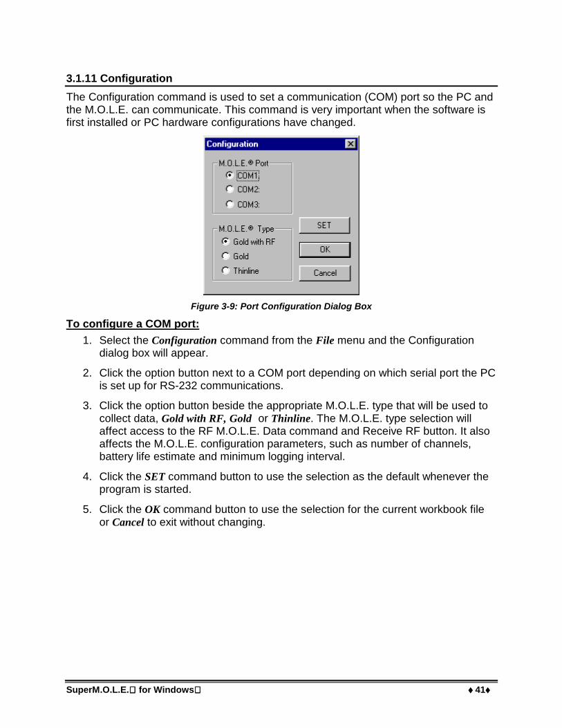
3.1.11 Configuration
The Configuration command is used to set a communication (COM) port so the PC andthe M.O.L.E. can communicate. This command is very important when the software isfirst installed or PC hardware configurations have changed.
Figure 3-9: Port Configuration Dialog Box
To configure a COM port:
1. Select the Configuration command from the File menu and the Configurationdialog box will appear.
2. Click the option button next to a COM port depending on which serial port the PCis set up for RS-232 communications.
3. Click the option button beside the appropriate M.O.L.E. type that will be used tocollect data, Gold with RF, Gold or Thinline. The M.O.L.E. type selection willaffect access to the RF M.O.L.E. Data command and Receive RF button. It alsoaffects the M.O.L.E. configuration parameters, such as number of channels,battery life estimate and minimum logging interval.
4. Click the SET command button to use the selection as the default whenever theprogram is started.
5. Click the OK command button to use the selection for the current workbook fileor Cancel to exit without changing.

♦♦♦♦ 42♦♦♦♦ SuperM.O.L.E. for Windows
3.1.12 List-Print Data
The List-Print Data command is used to display the raw data used to graph the DataPlots and calculate the statistics. Use this command to display data on the screen orcreate a new file with a file extension of (.PRN) that can be opened with wordprocessor, spreadsheet, or database programs.
The table of values that SMFW displays shows the X-value in the units currently set.The Negative X-values in the table indicate those that are to the left of the ProcessOrigin in the Data Graph. The next six columns include the Y-value for the channels ofdata collected by the M.O.L.E. in °F or °C, depending on the currently set units.
Figure 3-10: List Print Data Dialog Box
All or parts of the data can be List Printed by selecting a limited range of data to print.To do this, use the Magnify command from the Tools menu along with the List-Printcommand (refer to section 3.7.1 Magnify Tool for details).
This command can also be used by pressing CTRL + L.

SuperM.O.L.E. for Windows ♦♦♦♦ 43♦♦♦♦
3.1.13 Page Setup
The Page Setup command sets page parameters for the Finder worksheet.
Figure 3-11: Page Setup Dialog Box
To set the Finder page parameters:
1. Select the Page Setup command from the File menu.
2. Select desired parameters to apply to the worksheet.
3. Click the OK command button to use the current page setup selections.
4. Click the Cancel command button to leave the page setup command withoutchanging anything.
Selections made using the Page Setup command will not be visible on theworksheet it is only used for print formatting. To view the selections, use the PrintPreview command decsribed in section 3.1.16 Print Preview.

♦♦♦♦ 44♦♦♦♦ SuperM.O.L.E. for Windows
3.1.14 Print Options
The Print Options command is where additional Data Table statistics can be printedalong with the Main Plot is selected. Additional documentation can also be selected thatwill be printed on a second page.
Figure 3-12: Print Options Dialog Box
To select print options:
1. Select the Print Options command from the File menu.
2. Click the check box beside desired Statistic(s) to be printed along with the MainPlot.
3. Click the check box beside desired documentation to be printed on a secondpage.
• Click the Print command button to close the print options process and initiateprinting.
• Click the Print Preview command button to view the report appearance.
• Click the Set command button to save the current report options as thedefault, whenever the program is started.
• Click the OK command button to save the selected Print Options for thecurrent workbook file until it is closed or exited.
• Click the Cancel command button to leave the print options command withoutmaking any changes.
This command can also be used by pressing CTRL + R.

SuperM.O.L.E. for Windows ♦♦♦♦ 45♦♦♦♦
3.1.15 Page Header / Footer
The Page Header / Footer command places text on the top and bottom of the printedworksheet.
Some of the worksheets contain default information in the Header and Footerfields, to view use the Print Preview command. Refer to section 3.1.16 PrintPreview).
Figure 3-13: Header / Footer Dialog Box
To add a Header and/or Footer
1. Select the Page Header/Footer command from the File menu.
2. Click the Header tab or the Footer tab.
3. Determine where to locate the text: left, center or right side of the worksheet.Click a text field and type the desired text.
• The user can also change the text font, distance the note is from the frameedges and type of page numbering (refer to Figure 3-12).
4. Click the OK command button to accept the Header / Footer or click Cancel toreturn to the worksheet without changes.
The Header / Footer information will not be visible on the worksheet. It is onlyused for printing. To view the Header / Footer information, use the Print Previewcommand (refer to section 3.1.16 Print Preview).

♦♦♦♦ 46♦♦♦♦ SuperM.O.L.E. for Windows
3.1.16 Print Preview
The Print Preview command shows a preview of the page(s) to be printed. Thiscommand is useful when confirming print options.
To view a print preview:
1. Select the Print Preview command from the File menu and the Print Previewwindow will appear.
Figure 3-14: Print Preview Window
2. Click the Print command button to proceed with printing.
3. Click the Two-Page command button when there is more than one page in thereport to view them side by side.
4. Click the Next Page or Prev Page command button to view other pages of amultiple page report.
5. Click the Zoom In command button to observe small details, and Zoom Out torestore.
6. Click the Close command button to close the Print Preview window.

SuperM.O.L.E. for Windows ♦♦♦♦ 47♦♦♦♦
3.1.17 Print
The Print command prints worksheet information from the workbook. The options thatappear on the Print dialog box will depend on the type of printer and the printer driver.
To print a worksheet:
1. Select the Print command from the File menu and standard Windows or driver-dependent print dialog box will appear.
2. Select desired print options.
Figure 3-15: Print Dialog Box
3. Click the OK command button to close the Print dialog box and initiate printingthe worksheet.
4. Click the Cancel command button to close the print window without printing.
The Print command can be accessed on all worksheet Toolbars This command canalso be used by pressing CTRL + P.
• Print Button:

♦♦♦♦ 48♦♦♦♦ SuperM.O.L.E. for Windows
3.1.18 Report Setup
Select the Print Report command from the File menu to print the selected worksheetsfrom the Report worksheet as discussed in section 3.1.16 Print Preview.
To setup a report:
1. Select the Report Setup command from the File menu and a dialog box shown inFigure 3-16 will appear.
Figure 3-16: Report Setup Dialog Box
2. Click the check box(es) to enable the worksheet(s) to be printed.
3. Click the OK command button to accept the selection(s) and return to theworksheet, or click Cancel to return to the worksheet without any changes.

SuperM.O.L.E. for Windows ♦♦♦♦ 49♦♦♦♦
3.1.19 File Viewer
The File Viewer dialog box displays small thumbnail views of the graphical contents ofup to 120 data runs at one time. To select a data run, directly double click the desiredthumbnail graph box. This will automatically load the selected data run into the DataGraph.
Figure 3-17: File Viewer Window
How the data runs are displayed can be selected by pressing the command buttons onthe lower end of the dialog box. The user may select command buttons to Clear All,Clear Dups (Duplicates) Alpha Sort (by name) or Date Sort (by date profiled). Thethumbnail graphs may also be arranged by clicking on a selected graph and thendragging it to another location within the selected grid. When it is being moved to a newlocation, a dashed box will appear around the graph. Changing the arrangement in thismanner is temporary and the thumbnail graphs will return to the default locations whenthe dialog box is closed.
♦♦♦♦ 50♦♦♦♦ SuperM.O.L.E. for Windows
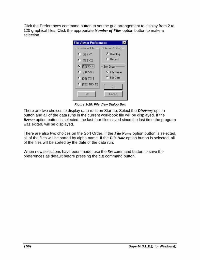
Click the Preferences command button to set the grid arrangement to display from 2 to120 graphical files. Click the appropriate Number of Files option button to make aselection.
Figure 3-18: File View Dialog Box
There are two choices to display data runs on Startup. Select the Directory optionbutton and all of the data runs in the current workbook file will be displayed. If theRecent option button is selected, the last four files saved since the last time the programwas exited, will be displayed.
There are also two choices on the Sort Order. If the File Name option button is selected,all of the files will be sorted by alpha name. If the File Date option button is selected, allof the files will be sorted by the date of the data run.
When new selections have been made, use the Set command button to save thepreferences as default before pressing the OK command button.

SuperM.O.L.E. for Windows ♦♦♦♦ 51♦♦♦♦
3.1.20 Print Report
Select the Print Report command from the File menu to print the selected worksheetsfrom the Report Setup dialog box as discussed in section 3.1.18 Report Setup.
3.1.21 Recent Files 1, 2, 3, etc...
The most recently loaded workbook file names are displayed at the bottom of the Filemenu. To open one of these files, click the name of the desired workbook file or pressthe appropriate number beside it.
3.1.22 Exit
Select the Exit command to quit the SMFW program. A message box will prompt theuser to save changes. If the user decides to save the changes, all data andconfiguration changes will be saved with the workbook file.
3.1.23 Language
All of the menus and commands have been translated in five different languages. Whenthe software is installed, a dialog box appears prompting the user to select a preferredlanguage. After the software is installed, the user can select a different language fromthe Languages sub-menu in the File menu.
Figure 3-19: Language Sub-Menu
Selecting a different language will not affect the Help command. Help is inenglish only.

♦♦♦♦ 52♦♦♦♦ SuperM.O.L.E. for Windows
3.2 Edit Menu
The Edit menu commands enable the user to modify the data set on the Finderworksheet so the most beneficial data is assembled in the workbook file.
3.2.1 Undo
Select the Undo command to undo any previous action. For example if the filtercommand is used and then the user decides that command was not necessary, theUndo command will restore it back to its original format.
The Undo command can be accessed on the Toolbar of the Finder worksheet. Thiscommand can also be used by pressing CTRL + Z.
• Undo Button:
3.2.2 Redo
Select the Redo command to restore the action made by using the Undo command. LikeUndo, the user can use Redo to restore all of the Undo actions.
The Redo command can be accessed on the Toolbar of the Finder worksheet. Thiscommand can also be used by pressing CTRL + R.
• Redo Button:
3.2.3 Remove Row
Select the Remove Row command to remove a data run row that is not wanted. Thiscommand is helpful when data has been collected and the user feels it is not beneficialto the workbook data set.
This command is permanent and the data run cannot be retrieved. The softwareprogram will warn the user with a message box.
3.2.4 Hide Row
Select the Hide Row command to exclude a row without eliminating it completely fromthe workbook file when analyzing the uploaded data run. This command is similar to thefilter function, and is helpful when data has been collected and it may not be beneficialto the data set. To restore hidden data set row(s) click the Red Filter Reset buttonlocated on the Finder worksheet (refer to section 2.2.7 Filters).

SuperM.O.L.E. for Windows ♦♦♦♦ 53♦♦♦♦
3.3 View Menu
The View menu commands enable the user to manipulate which areas are viewed onthe worksheet display.
3.3.1 Toolbar
Select the Toolbar command from the View menu to activate or deactivate the toolbar.When the Toolbar is deactivated, more of the worksheet area appears on the PCdisplay. When there is a checkmark beside the Toolbar command it is activated andwhen the checkmark is not there it is deactivated.
3.3.2 Status Bar
Select the Status bar command from the View menu to activate or deactivate the Statusbar on the bottom of the worksheets. When the Status Bar is deactivated, more of theworksheet area appears on the PC display. When there is a checkmark beside theStatus bar command it is activated and when the checkmark is not there it isdeactivated.
3.3.3 Zoom In
Select the Zoom In command from the View menu to make the current worksheet viewlarger. The Zoom In command has the capability to zoom in multiple times. When themaximum zoom level has been reached the Zoom In command will be dimmed.
The Zoom In command can be accessed on the Toolbars of the Welcome and Finderworksheets. This button will speed up the Zoom In process if multiple zooms aredesired.
• Zoom In Button:
3.3.4 Zoom Out
Select the Zoom Out command from the View menu to make the current worksheet viewsmaller. The Zoom Out command has the capability to zoom out multiple times. Whenthe minimum zoom has been reached the Zoom Out command will be dimmed.
The Zoom Out command can be accessed on the Welcome and Finder worksheets.This button will speed up the Zoom Out process if multiple zooms are desired.
• Zoom Out Button:

♦♦♦♦ 54♦♦♦♦ SuperM.O.L.E. for Windows
3.3.5 100%
Select the 100% command from the View menu to return the worksheet to its defaultdisplay size.
The 100% command can be accessed on the Toolbar of the Welcome and Finderworksheets.
• 100% Button:

SuperM.O.L.E. for Windows ♦♦♦♦ 55♦♦♦♦
3.4 Format Menu
The Format menu includes commands that change the layout or pattern of the text inuser configurable cells.
3.4.1 Bold
Select the Bold command from the Format menu to turn data in a user configurable cellbold. Select the Bold command again to return to standard format.
The Bold command can be accessed on the Toolbar of the Finder worksheet.
• Bold Button:
3.4.2 Italic
Select the Italic command from the Format menu to turn data in a user configurable cellitalic. Select the Italic command again to return to standard format.
The Italic command can be accessed on the Toolbar of the Finder worksheet.
• Italic Button:
3.4.3 Underline
Select the Underline command from the Format menu to underline data in a userconfigurable cell. Select the underline command again to return to standard format.
The Underline command can be accessed on the Toolbar of the Finder worksheet.
• Underline Button:
3.4.4 Alignment (Left, Center, Right)
Select the Left, Center or Right command from the Format menu to align data in a userconfigurable cell.
The alignment commands can be accessed on the Toolbar of the Finder worksheet.
• Alignment Buttons: , , (Align Left, Center, and Align Right)

♦♦♦♦ 56♦♦♦♦ SuperM.O.L.E. for Windows
3.5 Profile Menu
The Profile menu includes special commands specifically used on the Profileworksheet. Commands in this menu enable the user to view and edit experimentaldocumentation, change the appearance of the display and design experiments.
3.5.1 Part
Part documentation is information about the part being profiled. There are also fields forentering the date the data was recorded, a user name, part number or identification ofthe component being profiled. To enter Part documentation select the Part commandfrom the Profile menu and a dialog box will appear (See Figure 3-20).
The part date field automatically updates when reading data from the M.O.L.E.
Figure 3-20: Part Dialog Box

SuperM.O.L.E. for Windows ♦♦♦♦ 57♦♦♦♦
3.5.2 Process
Select the Process command from the Profile menu to enter and edit information aboutthe process that generated the profile data.
Figure 3-21: Process Dialog Box

♦♦♦♦ 58♦♦♦♦ SuperM.O.L.E. for Windows
3.5.3 Sensors
Select the Sensors command from the Profile menu to enter and edit information aboutthe sensor locations that are used to generate the profile data. The Thermocoupleplacement information entered in the T/C-Location cells are also displayed as the SensorLocations in the Data Table.
Figure 3-22: Sensor Location Descriptions

SuperM.O.L.E. for Windows ♦♦♦♦ 59♦♦♦♦
Select the Location Positions tab to enter sensor location options. The sensor locationoptions record the actual physical locations of the sensors, board size and appearanceinformation.
Location dimensions can also be entered in a number of unit types. Locations can beentered by typing in dimensions, or by dragging the sensor locations around on theimage. Note that X-dimensions are measured from the leading (right) edge or the firstedge to enter the process, and Y dimensions are from the top down.
X-dimensions, are also the same dimensions that are used by the Channel Lagcommand to re-align the profile lines if Lag is enabled (refer to section 3.5.4Channel Lag).
To select an image:
1. Select the Open command button to add or change the image file. When thisfield is activated, a list box will appear prompting the user to select an image file.The image files supported by the software are Dib-(.dib), Gif (.gif), Pcx (.pcx), Tiff(.tif), Targa (.tga), Bitmap (.bmp) and Jpeg (.jpg).
Figure 3-23: Sensor Location Positions
2. Click the OK command button to accept the additions/changes or click Cancel toreturn to the Profile worksheet without making any additions/changes.
Once an image (picture) is selected, copy of that image is added to the SMFW“Images” folder. This enables the user to easily locate any image or logo files.

♦♦♦♦ 60♦♦♦♦ SuperM.O.L.E. for Windows
Select the Channel Lag tab to access the channel lag dialog box. (Refer to section 3.5.4Channel Lag for more information).
Channel Lag dimensions, are also the same dimensions that are used by theLocation Positions options as X-Dimensions (See Figure 3-24).
Figure 3-24: Sensor Channel Lag

SuperM.O.L.E. for Windows ♦♦♦♦ 61♦♦♦♦
3.5.4 Channel Lag
Select the Channel Lag command from the Profile menu to enter the difference betweenthe distance from one sensor to another along a conveyorized system.
Figure 3-25: Channel Lag Dialog Box
On the dialog box, CH1 through CH6 represent each channel attached to the M.O.L.E.Click a option button beside an unit of measure and then enter the distance betweensensors.
If sensors are placed along a line in a process so they enter and exit oven zones atdifferent times, the resulting Data Plots lag behind one another. SMFW uses channellag information entered here to align the Data Plots so the results can be easilycompared during analysis.
To enable the Channel Lag command, click the Show Lag check box.

♦♦♦♦ 62♦♦♦♦ SuperM.O.L.E. for Windows
When the Channel Lag command is enabled, a small triangle will appear on the lowerend of the process origin line.
CHANNEL LAG INDICATOR
Figure 3-26: Channel Lag Indicator
Click the OK command button to return to the Profile worksheet using the new settingsor Cancel to return making no changes.

SuperM.O.L.E. for Windows ♦♦♦♦ 63♦♦♦♦
3.5.5 Units
The Units command is where the unit type for the X-axis is selected.
To select a X axis unit:
1. Select the Units command from the Profile menu and the Units dialog box willappear (See Figure 3-27).
Figure 3-27: Units Dialog Box
2. Click the option button beside Point, Time-Relative, Time-Absolute or Distance toselect the units for the X-axis.
• Point: the data points collected from the Process-Origin.
• Time-Relative: Time measured from the Process-Origin
• Time-Absolute: Time of day
• Distance: Distance from the Process Origin (Meters, Centimeters, Feet orInches).
3. Click the Fahrenheit or Celsius option button to represent the degrees for the Y-axis.
4. Click the OK command button to return to the Profile worksheet using the newsettings or Cancel to make no new changes.

♦♦♦♦ 64♦♦♦♦ SuperM.O.L.E. for Windows
3.5.6 Scaling
The Scaling command controls the scale of the X and Y axis units of the Data Graph onthe Profile worksheet.
To use the scaling command:
1. Select the Scaling command from the Profile menu, and the scaling dialog boxwill appear. This dialog box identifies the current settings of the displayed Y-axisunits and the maximum and minimum values of the Y-axis.
2. Select between Auto or Manual mode. In Auto mode, SMFW selects the scale ofthe Y-Axis to ensure all values are visible in the Profile worksheet. In Manualmode, the range of values for the Y-Axis must be manually set.
Figure 3-28: Scaling Dialog Box
3. Click the OK button to use the new settings or Cancel to return to the Profileworksheet with no changes.
The Scaling command is not avalible if the Data Graph has been magnified.

SuperM.O.L.E. for Windows ♦♦♦♦ 65♦♦♦♦
3.5.7 Temp Ref Lines (Temperature Reference Lines)
Temperature Reference Lines are colored horizontal lines and can be positionedanywhere within the range of Y-values in the graph using the Temp Ref Lines commandin the Profile menu.
Temperature Reference Lines are used for analysis when the T Above Ref(Time above the Reference Line) statistic is active (refer to section 2.3.9.3 T AboveRef)
Figure 3-29: Temp Ref Lines Dialog Box
The Temp Ref Lines dialog box identifies the units of the Y-axis and the current valuesof any Temperature reference lines in the Data Graph. Temperature reference lines canbe added or changed at any time and must be created before the T Above Ref statisticwill produce valid data in the Data Table.
To add Temperature Reference Lines to the Data Graph:
1. Select the Temp Ref Lines command from the Profile menu.
2. Click the check box above Low, Med, or Hi to draw that line in the graph.
3. Enter Y-axis value(s) by adjusting the slider position or typing it in the text box.
4. Click the OK command to return to the Profile worksheet using the new settingsor Cancel to not make any changes.

♦♦♦♦ 66♦♦♦♦ SuperM.O.L.E. for Windows
3.5.8 Oven Configure
The Oven Configure command, includes options that display details of the experimentand establish analysis criteria. These options also enable the user to create a model ofan ideal process that SMFW uses to compare to experimental conditions.
Figure 3-30: Oven Configure Dialog Box
The following information describes the options on the Oven Configure dialog box thatassist the user to set an oven.

SuperM.O.L.E. for Windows ♦♦♦♦ 67♦♦♦♦
•••• Zone Configuration
The Zone Configuration portion of the Oven Configuration dialog box defines thenumber of zones activated; color, name and length for each desired Zone.
Figure 3-31: Zone Configuration Options
When the zones are displayed in the Data Graph, the Zone Slope statistic can be usedbased on the zones defined with this dialog box. The zones can be changed at any timeby using the cells in this dialog box or changing them in the Zone Matrix (refer tosection 2.3.10.10 Zone Matrix for more details).

♦♦♦♦ 68♦♦♦♦ SuperM.O.L.E. for Windows
To define zones:
1. Select the Oven Configure command from the Profile menu.
Figure 3-32: Oven Configure Dialog Box
2. Click the corresponding check box beside a zone to activate or deactivate it.
3. Click the corresponding Color cell to select a custom color for that zone. Torestore to the default colors click the Default Colors command button.
4. Click the corresponding Name cell to enter a custom zone name if desired.
5. Click the option button beside the appropriate units of length or time for theprocess. Select between units of length: meters, centimeters, feet, inches orbetween units of time: hours or minutes.
6. Click the corresponding Length cell to enter a specific zone length for each zone.
7. Click the Show Zones command button to display the zones as colored bars alongthe X-axis.
8. Click the Zone Temp Matrix check box to activate the Zone Matrix.
9. Click the OK command button to create the zone(s) and close the Oven Configuredialog box or Cancel to quit without making any changes.

SuperM.O.L.E. for Windows ♦♦♦♦ 69♦♦♦♦
•••• Temperatures
After zone sizes are defined, the zone temperatures can be set. These temperaturescould be the upper and lower thresholds of acceptable temperatures to meet processstandards, temperature settings of upper and lower heat sources, or they could haveany meaning desired.
Figure 3-33: Zone Temperature Section
Use actual oven settings for each zone to use the Prediction tool.
To set zone temperatures:
1. Select the Oven Configure command from the Profile menu.
2. Click the top and bottom text field(s) to enter upper and lower zone temperaturesas a colored line for each zone of the Data Graph. The upper zone temperaturesappear as solid lines and the lower zones appear as dotted lines.
This matrix can be used to plot predicted data lines based on different zonetemperatures or conveyor rates. (Refer to section 3.7.9 Prediction Tool for adescription of this process.)
3. Click the OK command button to create the zone temperatures and close theOven Configure dialog box or click Cancel to quit without making any changes.

♦♦♦♦ 70♦♦♦♦ SuperM.O.L.E. for Windows
•••• Conveyor speed
Actual speed of the conveyor can be set using the Conveyor speed portion of the OvenConfigure dialog box. SMFW uses this value to calculate the X-axis values when aDistance option button has been selected. This number is also used as the actualconveyor speed that SMFW uses when prediction data lines are added. (Refer tosection 3.7.9 Prediction Tool).
Figure 3-34: Conveyor Speed Options
Conveyor Speed can not be set or viewed after the Data Graph has beenmagnified.
To set the conveyor speed:
1. Select the Oven Configure command from the Profile menu.
2. Enter the Conveyor Speed in the text box. This value will appear in the ZoneMatrix.
3. Select the option button beside the desired units such as: Distance (inches) perTime (Minutes).
4. Click the OK command button to return to the Data Graph using the new settingsor Cancel to return to the Data Graph with no changes.
Set conveyor speed to zero for batch processes where time units is selected forzone sizes.
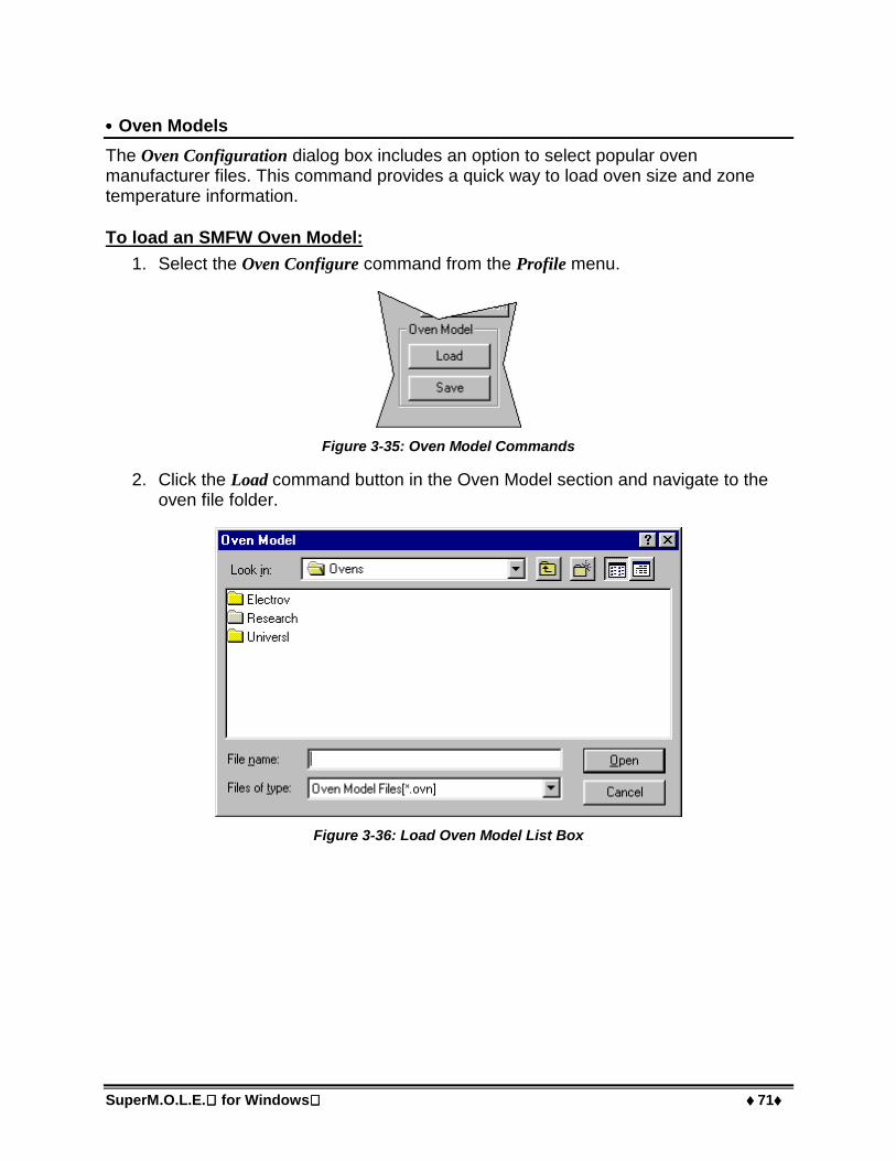
SuperM.O.L.E. for Windows ♦♦♦♦ 71♦♦♦♦
•••• Oven Models
The Oven Configuration dialog box includes an option to select popular ovenmanufacturer files. This command provides a quick way to load oven size and zonetemperature information.
To load an SMFW Oven Model:
1. Select the Oven Configure command from the Profile menu.
Figure 3-35: Oven Model Commands
2. Click the Load command button in the Oven Model section and navigate to theoven file folder.
Figure 3-36: Load Oven Model List Box

♦♦♦♦ 72♦♦♦♦ SuperM.O.L.E. for Windows
4. Select the desired manufacturer’s file folder.
Figure 3-37: Oven Model List Box
5. Select the desired oven model by clicking it once.
6. Click the Open command button.
Loading an oven model will overlay the current data set with the following informationfrom the Oven Model File:
• Zone Size Information
• Zone Temperature Information
• Conveyor Speed Information
• Process notes if the existing file has process information.
SuperM.O.L.E. for Windows ♦♦♦♦ 73♦♦♦♦
Creating and Saving an Oven Model:
1. Make sure current data is saved.
2. Edit the following information to fit the desired requirements. Zone Sizes, ZoneTemperatures, Conveyor Speed (from the Oven Configuration Dialog Box) andPart, Process, Sensor Documentation (from the Profile menu).
3. Select the Oven Configuration command from the Profile menu.
4. Click the Save command button from the Oven Model section and navigate to theOvens file folder.
5. Select the file folder of an oven manufacturer. (Additional file folders may becreated if needed).
6. Enter the file name in the File name text box. The extension assigned to this fileis (.OVN).
7. Click the Save command button.
The new Oven Model is now ready to use
Process information will only be used if there is no process information in thedata set that exists when a Oven Model is loaded.

♦♦♦♦ 74♦♦♦♦ SuperM.O.L.E. for Windows
3.5.9 Zone Matrix
To view the Zone Matrix, select the Zone Matrix command from the Profile menu andcheck mark will appear beside it to indicate that the Zone Matrix is activated. When theZone Matrix is turned “ON”, it is located above the Data Graph.
The Zone Matrix command can be accessed on the Profile worksheet Toolbar.
• Zone Matrix Button:
3.5.10 Calculate h-Factor
The h-Factor command is used along with an optional h-Factor module to measure anoven's ability to heat items passing through it. It is most useful in processes whereconstant, uniform temperatures are desirable.
Figure 3-38: Calculate h-Factor Dialog Box
Cure Factor Setup
1. Attach the optional h-Factor module to the M.O.L.E. thermocouple inputchannels 1 through 4 and use the options in Figure 3-38 to:
• Set the h-Constant, this is the calibration constant for that module.
If the wrong h-Constant is used, the resulting readout is incorrect.
2. Click OK to return to the Data Graph using the new settings or Cancel to return tothe Data Graph with no changes.

SuperM.O.L.E. for Windows ♦♦♦♦ 75♦♦♦♦
3.5.11 Profile Defaults Sub-Menu
The Profile Defaults sub-menu commands sets Profile menu commands with standarddefaults. When an option in the Defaults sub-menu is selected and a value is changed,the new value becomes the default that is used when a new workbook file is created.Default values are applied when importing old data files because they may not containall the information needed by SMFW.
To create new defaults:
1. Select a command from the Profile Defaults sub-menu.
2. Change the default setting(s).
3. Click the SET command button on the specific dialog box to save the new defaultsetting(s).
Typically the defaults are set once for specific requirements and cloned afterwards.Profile defaults are then changed only when requirements change.

♦♦♦♦ 76♦♦♦♦ SuperM.O.L.E. for Windows
3.6 M.O.L.E. Menu
The M.O.L.E. menu commands configure the M.O.L.E. for collecting data, and to read itafter data collection.
The M.O.L.E. must be connected to a PC and the proper communication portmust be configured to properly use the M.O.L.E. menu commands (refer tosection 3.1.11 Configuration).
3.6.1 Set M.O.L.E. Clock
The M.O.L.E. has an internal clock it uses to identify the time and date of each data runand to control when each measurement is recorded. The M.O.L.E. clock should be setprior to data collection to ensure that the proper time was recorded.
Figure 3-39: Set M.O.L.E. Clock Dialog Box

SuperM.O.L.E. for Windows ♦♦♦♦ 77♦♦♦♦
To set the M.O.L.E. clock:
1. Connect the M.O.L.E. to the PC (refer to the appropriate section in the Hardwaremanual).
2. Select the Set M.O.L.E. Clock command from the M.O.L.E. menu.
3. Enter the correct month, day, year, hour, minute, and second by adjusting theslider(s) or manually typing in the corresponding text box.
When the Set M.O.L.E. Clock dialog box appears the current computer clocksetting is automatically entered in the text boxes.
4. Click the Send button to reset the clock.
To read the M.O.L.E. clock:
1. Connect the M.O.L.E. to the PC (refer to the appropriate section in the Hardwaremanual).
2. Select the Set M.O.L.E. Clock command from the M.O.L.E. menu.
3. Click the Read command button to display the current date and time from theM.O.L.E.. If the clock is set wrong, the date or time will be incorrect.

♦♦♦♦ 78♦♦♦♦ SuperM.O.L.E. for Windows
3.6.2 M.O.L.E. Configure
The M.O.L.E. Configure command configures how the M.O.L.E. records data during adata run.
Figure 3-40: M.O.L.E. Configure Dialog Box
To configure the M.O.L.E.:
1. Select the M.O.L.E. Configure command from the M.O.L.E. menu.
2. Click the check box beside a corresponding channel to turn it “ON” or “OFF”. If achannel is “OFF”, it does not collect data or draw power from the battery.
3. Enter an interval at which the M.O.L.E. records data points by using the slider(s)or manually typing in the corresponding text box. The maximum interval for theM.O.L.E. is 23:59:59 hours (one data point per day) and the minimum interval is0.2 second (one data point every two-tenths of a second). When using theM.O.L.E. with RF Option the minimum interval is 0.5 (one data point every five-tenths of a second) and when one channel is active, the minimum interval is 0.1second (one data point every tenth of a second).
4. Enter the number of data points the M.O.L.E. will record during the data run. Themaximum number is dependent on the number of channels turned on. Themaximum data points the M.O.L.E. can collect are displayed above the text box.When the number of data points collected and the recording interval have beenselected, SMFW displays the corresponding time the experiment will take besideTotal Time = text in the lower right corner of the dialog box.

SuperM.O.L.E. for Windows ♦♦♦♦ 79♦♦♦♦
When M.O.L.E. configure options are modified, the data is calculated and thenamount of profiles the user can expect from the power pack battery (based on afully-charged power pack battery) is displayed in the lower right corner next tothe Profiles Per Battery line.
Optional configurations:
• Enter a threshold temperature to “trigger” the M.O.L.E. to start recording data byusing the slider or by entering it in the text box. When any active channelreaches that temperature, the M.O.L.E. will begin to record data. This option cantrigger the profiler when the temperature cools down to the thresholdtemperature by selecting the (-) option button, or heating up to the thresholdtemperature by selecting the (+) option button. If this option is not used fortemperature triggering, select the Off option button.
• Enter how many data points to delay “trigger” the M.O.L.E. to start recording databy using the slider or by entering it in the text box. The data point entered will“trigger” the start of data collection when the specified data point is reached inthe process. The actual delay is equal to the Interval times the Pts Dly.
5. Connect the M.O.L.E. to the PC (refer to the appropriate section in the Hardwaremanual).
6. Click the Send command button to send the new configurations to the M.O.L.E.
7. Click the Read command button to confirm the active configuration.
8. Click the OK command button to return to the Data Graph, retaining any changesmade to the configuration or Cancel to return to the Data Graph without recordingany changes.
The M.O.L.E. configure command can be accessed on the Toolbars of the Finder andProfile worksheets.
• M.O.L.E. Configure Button:

♦♦♦♦ 80♦♦♦♦ SuperM.O.L.E. for Windows
3.6.3 RF M.O.L.E. Data
This command activates SMFW to receive “Real-time” data from the M.O.L.E. whenusing it with the RF option.
To Read RF M.O.L.E. Data:
1. Connect the RF Receiver to the PC using the interface cable supplied (refer tothe appropriate section in the Hardware manual).
2. Select the RF M.O.L.E. Data command from the M.O.L.E. menu. A message boxwill appear asking the user if they want to start a new experiment file.
Figure 3-41
• Click the Yes command button to start the new data run using default settings.
• Click the No command button to receive data into the current data run row.
• Click the Cancel command button to return to the Data Graph without receivingM.O.L.E. RF data.
3. If Yes is selected, a message box will appear asking the user if they want to clonethe existing experiment information.
Figure 3-42
• Click the Yes command button to start the new data run using the currentsettings.
• Click the No command button to start the new data run using the default settings.
• Click the Cancel command button to return to the Data Graph without receivingM.O.L.E. RF data.

SuperM.O.L.E. for Windows ♦♦♦♦ 81♦♦♦♦
4. If either the Yes or No command button is selected the Read Data from RFM.O.L.E. dialog box will appear and “Real-time” data will start to appear on thelower edge of the dialog box.
Figure 3-43: RF Dialog Box
5. Click the OK command button when finished collecting transmitted data and thedata run will automatically be uploaded into the workbook file.

♦♦♦♦ 82♦♦♦♦ SuperM.O.L.E. for Windows
If the computer is not communicating with the receiver, the message box shownin Figure 3-44 will appear. This message box is an indication of a cable or portconfiguration problem and not the transmitter. If this message does not appearand no data is received, refer to the RF Trouble Shooting section in the hardwaremanual for radio link trouble shooting hints.
Figure 3-44
If the PC interface cable is connected to the M.O.L.E. instead of the Receiver amessage box indicating the problem will appear.
The RF M.O.L.E. Data command can be accessed on all of the worksheet Toolbars.
• RF M.O.L.E. Data Button:

SuperM.O.L.E. for Windows ♦♦♦♦ 83♦♦♦♦
RF M.O.L.E. dialog box features:The RF M.O.L.E. Data dialog box has many features. Use the illustration shown inFigure 3-45 and the following definitions to interpret.
CHANNEL TEMPS.
ELAPSEDTIME
REMAINING PROFILE TIME
ALARM LOG
ALARM VISUAL INDICATORS
ALARM MESSAGE BOX
INTERNALTEMPERATURE
THERMOMETER
Figure 3-45: RF Dialog Box Features:
• Alarm Message Box - This indicates the last alarm point breached.
• Internal Temperature Thermometer - This is an indicator displaying the currentinternal temperature of the M.O.L.E..
• Remaining Profile Time - This is the amount of data collection time preset bythe user.
• Channel Temperatures - This displays the current temperature that the sensorsare reporting.
• Elapsed Time - This displays the elapsed time from when the data run hasbegun.
• Alarm Visual Indicators - When a user-preset temperature has been reached,the box of that alarm that has been reached will flash. This feature will bedimmed until it has been configured by the user (refer to Section 3.6.5.1 RFAlarm Points).
• Alarm Log - This is a drop down list box that logs the time and channel that hasbeen breached during the current profile.

♦♦♦♦ 84♦♦♦♦ SuperM.O.L.E. for Windows
3.6.4 Read M.O.L.E. Data
This command starts transferring a data run from the M.O.L.E..
To Read M.O.L.E. Data:
1. Connect the M.O.L.E. to the PC using the cable supplied (refer to theappropriate section in the Hardware manual).
2. Select the Read M.O.L.E. Data command from the M.O.L.E. menu. A messagebox will appear asking the user if they want to start a new experiment file.
Figure 3-46
• Click the Yes command button to start a new data run using default settings.
• Click the No command button to upload the data run into the current data runrow.
• Click the Cancel command button to return to the Data Graph without uploadingthe data run.
3. If Yes is selected, a message box will appear asking the user if they want to clonethe existing experiment information.
Figure 3-47
• Click the Yes command button to start uploading the data run using the currentsettings.
• Click the No command button to start uploading the data run using the defaultsettings.
• Click the Cancel command button to return to the Data Graph without uploadingthe data run.
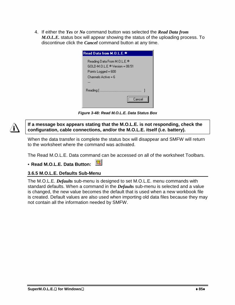
SuperM.O.L.E. for Windows ♦♦♦♦ 85♦♦♦♦
4. If either the Yes or No command button was selected the Read Data fromM.O.L.E. status box will appear showing the status of the uploading process. Todiscontinue click the Cancel command button at any time.
Figure 3-48: Read M.O.L.E. Data Status Box
If a message box appears stating that the M.O.L.E. is not responding, check theconfiguration, cable connections, and/or the M.O.L.E. itself (i.e. battery).
When the data transfer is complete the status box will disappear and SMFW will returnto the worksheet where the command was activated.
The Read M.O.L.E. Data command can be accessed on all of the worksheet Toolbars.
• Read M.O.L.E. Data Button:
3.6.5 M.O.L.E. Defaults Sub-Menu
The M.O.L.E. Defaults sub-menu is designed to set M.O.L.E. menu commands withstandard defaults. When a command in the Defaults sub-menu is selected and a valueis changed, the new value becomes the default that is used when a new workbook fileis created. Default values are also used when importing old data files because they maynot contain all the information needed by SMFW.

♦♦♦♦ 86♦♦♦♦ SuperM.O.L.E. for Windows
3.6.5.1 RF Alarm Points
While transmitting data with the M.O.L.E. RF Option, the RF Alarm Points commanddisplays a customized alert message informing the user that a preset temperature hasbeen met.
To use RF Alarm Points:
1. Select the RF Alarm Points command from the M.O.L.E. Defaults menu.
2. Select alarm(s) to activate, Low, Medium and/or High, by selecting the (+) =Rising temperature or (-) = Falling temperature option buttons.
3. Determine alarm point temperature(s) for the alarm points by adjusting the slideror typing in the corresponding text box.
4. Select which channel to apply the alarm(s) to.
5. Select a Message box and or an audio indication to alert the user when an alarmtemperature has been met.
6. Click the Set command button to set the current configuration as defaults orCancel to keep the previous settings.
Figure 3-49: RF Alarm Dialog Box

SuperM.O.L.E. for Windows ♦♦♦♦ 87♦♦♦♦
Alarm messages can be changed to indicate what the alarm message is describing.The default messages are Low Alarm, Medium Alarm and Hi Alarm.
To edit an alarm message:
1. Click an Edit Message command button.
Figure 3-50: RF Alarm Message Text Box
2. Enter custom message in the text box and click the OK command button toaccept or Cancel to not make any changes.
The results of programming RF Alarm points are used with the RF Option, and appearin the Read Data from RF M.O.L.E. dialog box while receiving data. (See Figure 3-51)
Figure 3-51: Alarm Message Box

♦♦♦♦ 88♦♦♦♦ SuperM.O.L.E. for Windows
3.7 Tools Menu
Options in this menu make it easy to deal with data files and change the appearance ofthe Data graph.
3.7.1 Magnify Tool
The Magnify tool enlarges any selected area of the data graph for easy visualexamination.
To Magnify a portion of the Data Graph:
1. Click the Magnify tool from the Tools menu. A message will appear in the toolstatus box indicating that “Magnify Tool” has been selected and informing theuser to “Click and drag to select area”.
2. Position the mouse pointer on a desired section of the Data Graph to select onecorner of the area to enlarge.
3. Press the left mouse button and drag the pointer diagonally to the oppositecorner of the box. An outline of the box appears as you drag.
4. Release the left mouse button when the outline of the area to be magnified isvisible. The area inside the box is then magnified to fill the entire Data Graph.

SuperM.O.L.E. for Windows ♦♦♦♦ 89♦♦♦♦
To show even more detail in the Data Graph, Magnify can be performed multiple times.If the Magnify tool reaches the maximum zoom capability the software will display amessage box informing that the user has “Zoomed to Tight”.
When using the Magnify tool, the Magnify Map uses a red box to indicate the areacurrently magnified. If the data graph was previously magnified, the current level ofmagnification is the red box and previous magnified areas are noted with gray boxes.
MAGNIFYMAP
MAGNIFIEDAREA
Figure 3-52: Magnify Map
When the Magnify tool has been used multiple times, click the Magnify map once to goback to a previously selected level of magnification.
Magnify Applications:Magnify is useful for visually examining data, such as with the Slope tool, and whenstatistics are used. The statistics (Value, Time to Ref., T Above Ref, and Statistics)compute only data points that fall within the area of the Data Graph. This enables theuser to focus the statistical analysis on any portion of time, distance, or data pointnumber in the graph.
The Magnify command can be accessed on the Profile worksheet Toolbar.
• Magnify Button:

♦♦♦♦ 90♦♦♦♦ SuperM.O.L.E. for Windows
3.7.2 Slope Tool
The Slope tool finds the average slope between any two points in the Data Graph.
To find the average slope of a line:
1. Select the Slope tool from the Tools menu. A message will appear in the toolstatus box indicating that the “Slope Tool” has been selected and reminding theuser to “Click and drag for slope”.
2. Position the mouse pointer at a point on the curve.
3. Press and hold the left mouse button. A new message will appear in the ToolStatus Box showing the Slope, the change in X in time, distance, or pointnumbers, and the change in Y in degrees. These numbers will change while theslope is being defined.
4. Drag the pointer to the end of the desired slope line.
5. Release the left mouse button when the pointer is at the desired location. SMFWwill draw a slope line on the Data Graph, and label the slope value.
SLOPEDATA
SLOPELINE
Figure 3-53: Slope Tool

SuperM.O.L.E. for Windows ♦♦♦♦ 91♦♦♦♦
To obtain more accurate slopes:Magnify a portion of the Data Graph using the Magnify tool, and repeat this procedure.
To remove the slope line from the Data Graph, select the Erase Object(s) command fromthe Tool menu and follow instructions in the Tool Status box (refer to section 3.7.11Erase Object(s)).
Slope Applications:Use the Slope tool to find the average slope between any two points on the graph.Longer slope lines tend to produce more accurate slope calculations.
The Slope tool can be used to compare actual data with ideal conditions by drawing aline with a known slope (to represent the ideal condition) beside a portion of a DataPlot.
Slope Limitations:Slope calculations are based on logged points connected by the slope line. Pointsoccur only at the exact time intervals used to record data.
The Slope tool cannot measure slopes when dx (change in X) is equal to zero (whenthe line is vertical).
The Slope tool can be accessed on the Profile worksheet Toolbar.
• Slope Button:

♦♦♦♦ 92♦♦♦♦ SuperM.O.L.E. for Windows
3.7.3 Peak Difference Tool
The Peak Difference tool displays the difference in value between the peak of themaximum Data Plot and the peak of the minimum Data Plot in any location of the DataGraph. This command is especially useful for measuring side-to-side heatingdifferences in ovens.
To display the peak difference between Data Plots:
1. Select the Peak Difference tool from the Profile menu and a message will appearin the tool status box indicating that the “Peak Difference Tool” has beenselected and reminding the user to “Click and drag to select an area”.
2. Position the mouse pointer over a location in the Data Graph.
3. Click and drag to select an area.
The peak difference is calculated as the maximum difference between the highest peakand the lowest peak within the rectangle.
To remove the peak difference rectangle and annotation from the Data Graph,select the Erase Objects command from the Tools menu and follow instructions inthe Tool status box (refer to section 3.7.11 Erase Object(s)).
PEAKDIFFERENCE
Figure 3-54: Peak Difference Tool
The Peak Difference tool can be accessed on the Profile worksheet Toolbar.
• Peak Difference Button:

SuperM.O.L.E. for Windows ♦♦♦♦ 93♦♦♦♦
3.7.4 Overlay Tool
The Overlay tool displays a second Data run graph for comparison with the currentlydisplayed Data run.
To compare two Data Plots:
1. Click the Overlay tool from the Tools menu. A list box of data files uploaded intothe opened workbook will appear.
2. Select a data run file to overlay on the original by clicking it.
The data file will be inserted at the same process origin and automatically scaled to thesame Y-axis. The original Data Plot remains as solid lines while those added forcomparison are dashed.
The dashed “Overlay” Data Plots are the same color as the original Data Plots.
Figure 3-55: Overlay Tool
To remove the overlaid Data Graph from the original Data Graph select theOverlay tool again or press the right mouse button.

♦♦♦♦ 94♦♦♦♦ SuperM.O.L.E. for Windows
The Overlay and Magnify tools can be used together to overlay and compare idealreference profiles and magnified portions of the two data files. They can have differentbut overlapping X-values (times, point numbers, logging intervals) or temperatures.
Overlay Limitations:If the Data Plots are too numerous to clearly see the information of interest, they can besuppressed by removing the check mark from the desired channel in one or both files.This must be done to the overlaid profile prior to using the Overlay tool. Save that graphand use the Overlay tool again.
The Overlay tool can be accessed on the Profile worksheet Toolbar.
• Overlay Button:

SuperM.O.L.E. for Windows ♦♦♦♦ 95♦♦♦♦
3.7.5 Total Heat Tool
The Total Heat tool computes the area between the Data Plot curves and the bottomborder of the selected Total Heat area. This can be used for easy evaluation of heatinput.
Total heat is calculated by multiplying the temperature difference at a given X-value bythe time between this X-value and the previous one or the area under the curve. Theunits are Degrees Seconds.
To evaluate the heat input for a specific portion of a Data Graph:
1. Select the Total Heat tool from the Tools menu. A message will appear in the toolstatus box indicating that the “Total Heat Tool” has been selected and remindingthe user to “Click and drag to select an area”.
2. Position the mouse pointer at an initial X/Y coordinate.
3. Press the left mouse button and drag diagonally. The outline of a box will appearas you drag.
4. Release the mouse button when the box reaches the second X/Y coordinate,enclosing the range of X/Y values that are included in the total heat calculation.

♦♦♦♦ 96♦♦♦♦ SuperM.O.L.E. for Windows
The area under Data Plot(s) and between the two X-boarders are calculated anddisplayed next to the Total Heat rectangle. The channel that is calculated at 100%, isthe channel with the highest total heat. The other channels have a calculated total heatpercentage of the 100% channel. The Data Graph displays the calculated areas byfilling in the area under the Data Plots.
TOTAL HEATRECTANGLE
Figure 3-56: Total Heat Tool
To remove the Total Heat object from the Data Graph, select the Erase Object commandfrom the Tools menu and follow instructions in the Tool status box (refer to section3.7.11 Erase Object(s)).
The bottom of the Total Heat box can be used at either 0°°°° or room temperature togive “Total” Heat calculations above 0°°°° or room temperature.
Total Heat Applications:The Total Heat tool is helpful to compare the heat input between two sensor channelsand averages the small local temperature differences. This tool is especially useful formeasuring side-to-side heating differences in ovens.
The Total Heat tool can be accessed on the Profile worksheet Toolbar.
• Total Heat Button:

SuperM.O.L.E. for Windows ♦♦♦♦ 97♦♦♦♦
3.7.6 3-D Tool
The 3-D tool draws a 3-dimensional representation of the temperature data. When the3-D tool is selected, a dialog box will appear prompting the user to select between a“Normal” or a “Reverse-Angle” view. A “Normal” view shows channel 1 in back andchannel 6 in front, and a “Reverse-Angle” view shows channel 6 in the back andchannel 1 in front.
The 3-D profile, shown below, is useful for comparing the general smoothness of theData Plots for each sensor or showing uniform heating across an oven.
Figure 3-57: Normal View

♦♦♦♦ 98♦♦♦♦ SuperM.O.L.E. for Windows
Figure 3-58: Reverse-Angle View
To remove the 3-D profile, click the 3D tool or click the right mouse button.
The 3-D tool can be accessed on the Profile worksheet Toolbar.
• 3-D Button:
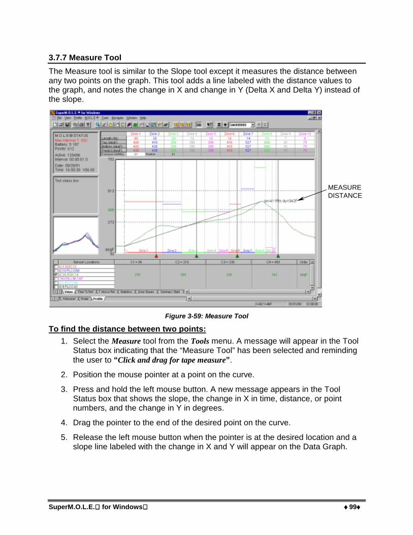
SuperM.O.L.E. for Windows ♦♦♦♦ 99♦♦♦♦
3.7.7 Measure Tool
The Measure tool is similar to the Slope tool except it measures the distance betweenany two points on the graph. This tool adds a line labeled with the distance values tothe graph, and notes the change in X and change in Y (Delta X and Delta Y) instead ofthe slope.
MEASUREDISTANCE
Figure 3-59: Measure Tool
To find the distance between two points:
1. Select the Measure tool from the Tools menu. A message will appear in the ToolStatus box indicating that the “Measure Tool” has been selected and remindingthe user to “Click and drag for tape measure”.
2. Position the mouse pointer at a point on the curve.
3. Press and hold the left mouse button. A new message appears in the ToolStatus box that shows the slope, the change in X in time, distance, or pointnumbers, and the change in Y in degrees.
4. Drag the pointer to the end of the desired point on the curve.
5. Release the left mouse button when the pointer is at the desired location and aslope line labeled with the change in X and Y will appear on the Data Graph.

♦♦♦♦ 100♦♦♦♦ SuperM.O.L.E. for Windows
To obtain more accurate distances, magnify a portion of the Data Graph using theMagnify tool and repeat this procedure.
To remove the annotated distance from the Data Graph, select the Erase Objectscommand from the Tools menu and follow instructions in the Tool Status box(refer to section 3.7.11 Erase Object(s)).
The Measure tool can be accessed on the Profile worksheet Toolbar.
• Measure Button:

SuperM.O.L.E. for Windows ♦♦♦♦ 101♦♦♦♦
3.7.8 Notes Tool
The Notes tool adds a leader with text to any portion on the graph to label special areasof interest.
To add notes to the Data Graph:
1. Select the Notes tool from the Tools menu. A message will appear in the toolstatus box indicating that the “Notes Tool” has been selected and reminding theuser to “Click and drag for pointer”.
2. Position the mouse pointer at the desired location to start the note leader, clickand drag the mouse pointer to the desired location of the note text and releasethe mouse button.
3. A dialog box will then appear allowing the user to enter a note by typing it in thetext box. There also are options to customize the color, border and font size ofthe notes.
Figure 3-60: Notes Dialog Box
4. Click the OK command button or press the [enter] key to finish adding the note.
To remove notes from the Data Graph, select the Erase Object command in theTools menu and follow instructions in the Tool Status box (refer to section 3.7.11Erase Object(s)).
The Notes tool can be accessed on the Profile worksheet Toolbar.
• Notes Button:

♦♦♦♦ 102♦♦♦♦ SuperM.O.L.E. for Windows
3.7.9 Prediction Tool
One of the most impressive features of SMFW is its Prediction tool. This tool enablesthe user to change a zone temperature value or the conveyor speed and predict theoutcome of that change. Prediction is easy to use and a valuable command that quicklydefines process parameters.
To use Prediction some information must first be entered into the Zone Matrix to buildan accurate “model” of an oven environment. As experience with modeling grows, thefirst values selected may need to be modified accurately reflect the process.
To model a process:
1. Complete a data run in an oven with a test assembly to establish a base line forthe process.
2. Enter zone sizes in the length fields for each zone. This is the length of eachheating, soaking, or cooling zone within the oven.
ZONE MATRIXZONE LENGTHS
ZONETEMPS
CONVEYORSPEED
Figure 3-61: Zone Matrix Data
Make sure the zones are visible by clicking the Show Zones check box on the OvenConfigure dialog. This enables the user to see how each heating zone affects theresults.

SuperM.O.L.E. for Windows ♦♦♦♦ 103♦♦♦♦
3. Enter the temperature for each zone by typing it in the temperature cells for eachzone on the Zone Matrix. This is the set temperature of each zone preset withinthe oven.
If there is a soak zone, then set it to the same temperature as the previous zone.
4. Enter a conveyor speed in the conveyor cell on the Zone Matrix. The conveyorrate documented for this experiment is displayed along with zone temperatures.
The units for the X-Cursor should be set to Distance. To set the units to distance,select the Units command from the Profile menu.
5. Move the Process Origin on the Data Graph to the place that corresponds to thebeginning of the oven. Typically, this is where all of the channel temperaturessuddenly rise. Now the prediction command is ready to use.

♦♦♦♦ 104♦♦♦♦ SuperM.O.L.E. for Windows
SMFW offers two ways to predict results:
Dialog box Prediction:
1. Select the Prediction tool from the Tools menu and the Oven dialog box willappear. The shaded portions of this dialog box indicate that they cannot bemodified by the user.
Figure 3-62: Oven Dialog Box
2. Enter a hypothetical conveyor speed and or zone temperature.
3. Click the Do Prediction command button and SMFW will calculate and plot thepredicted outcome based on the changed value(s). The predicted Data Plotsappear on the Data Graph as dashed lines. Use the Slope, Measure, andMagnify tools to see if the ideal profile has been achieved.
4. Experiment by making more “what if” changes to the conveyor speed, ortemperature values and replotting the prediction. Click the Reset Temps commandbutton to change zone temperatures back to the original oven values.
5. Set the oven to the final prediction values, and then perform another data run tocheck if the process has been optimized.
6. Select the Prediction command again and the original zone temperatures cannow be reset. Save the current prediction, proceed with another prediction, orclick the End Prediction command button to remove the predicted Data Plots.

SuperM.O.L.E. for Windows ♦♦♦♦ 105♦♦♦♦
Dynamic Prediction:
1. Select the Prediction tool from the Tools menu and the Oven dialog box willappear.
2. Click the Do Prediction command button on the Oven dialog box and the Datagraph will appear.
3. Move the mouse pointer over a Zone Temperature Prediction Handle.
ZONE TEMPERATUREPREDICTION HANDLES
Figure 3-63: Dynamic Prediction Feature
4. Press and hold the left mouse button to slide the handle up or down to thepreferred prediction temperature (repeat for other zones).
5. Set the oven to the final prediction values, and then perform another data run tocheck if the process has been optimized.
6. Select the Prediction command again and the original zone temperatures cannow be reset. Save the current prediction, proceed with another prediction, orclick the End Prediction command button to remove the predicted Data Plots.

♦♦♦♦ 106♦♦♦♦ SuperM.O.L.E. for Windows
Saving a Predicted Profile:Prediction settings can also be saved by clicking the Save Prediction command button.
When prediction settings are saved, SMFW automatically saves the prediction profileas a new (.MDM) file. The predicted profile data is also loaded into the Finderworksheet as a data run labeled with a description, original data run and new Filename.
PREDICTIONLABEL
ORIGNALDATA RUN
PREDICTIONFILE
Figure 3-64: Saved Prediction
The Prediction tool can be accessed on the Profile worksheet Toolbar.
• Prediction Button:

SuperM.O.L.E. for Windows ♦♦♦♦ 107♦♦♦♦
Conflicting Conditions:If SMFW detects sensor temperatures inconsistent with zone temperature settings, amessage box with an explanation will appear. The explanation appears only once foreach zone, each time Prediction is used. After that, SMFW assumes the user is awareof the potential problem. There is also a basic prediction assumption that temperaturesare rising throughout the process, so any zone having a falling temperature will benoted.
ZONES WITHPOTENTIAL
PROBLEM
Figure 3-65: Conflicting Conditions Dialog Box
In the example, the message box displays a warning message and shows that zone twoand eight have a potential problem.
The inconsistent setting does not prevent SMFW from making a prediction it makes arational assumption about what is happening. In addition to the explanation, SMFWdisplays several logical ways to correct the conflicting conditions at the bottom of thedialog box.
If Zone temperatures are not set, the Prediction tool will not work.

♦♦♦♦ 108♦♦♦♦ SuperM.O.L.E. for Windows
3.7.10 Tolerance Band Tool
The Tolerance Band tool develops standard temperature profile bands that can be usedto determine compliance with required process limits.
To develop a tolerance band:
1. Select the Tolerance Band tool and the Tolerance Band dialog box will appear.
Figure 3-66: Tolerance Band Dialog Box
2. Select the check boxes next to the desired channels to apply the tolerance to.
Only active channels will be enabled.
3. Set the % Above with the slider bar or by typing a value in the text box. This valueis the percent (%) above the highest selected channel and % Below which is thepercent (%) below the lowest selected profile channel.

SuperM.O.L.E. for Windows ♦♦♦♦ 109♦♦♦♦
4. Click the Apply command button and the values for the Tolerance Band are nowcalculated and displayed on the Data Graph.
5. Click the OK command button to hide the Tolerance Band dialog box and viewthe applied tolerance band.
SMFW uses the maximum of the selected channel data values and then the percent(%) above is calculated for the upper value of the band. The lower value is calculated inthe same manner using the minimum of the channels selected and the percent (%)below. Once the band is defined, a line is drawn from the top to the bottom value ateach data point.
Figure 3-67: Tolerance Band
6. Click the Remove command button to remove the Tolerance Band from the DataGraph.
7. Click the Cancel command button to return to the Data Graph.

♦♦♦♦ 110♦♦♦♦ SuperM.O.L.E. for Windows
Once a Tolerance Band has been developed and applied, it can be saved as a copy forfuture retrieval from the SMFW Standards file folder. When the Tolerance band tool isbeing used an existing or previously defined Tolerance Band may be loaded by usingthe Open command button.
To Save a Tolerance band:
1. Click the Save command button on the Tolerance Band dialog box and a list boxwill appear.
Figure 3-68: Tolerance Band Save List Box
2. Enter a name in the File name text box. The Tolerance Band will be assigned thefile name extension (*.STD).
3. Click the Save command button to save or Cancel to return to the Tolerance Banddialog box.
To Open a tolerance band:
1. Click the Open command button on the Tolerance Band dialog box and a list boxwill appear.
2. Select a Tolerance Band file by clicking it.
3. Click the Open command button to apply the saved tolerance or Cancel to returnto the Tolerance Band dialog box.
The Tolerance Band tool can be accessed on the Profile worksheet Toolbar.
• Tolerance Band Button:

SuperM.O.L.E. for Windows ♦♦♦♦ 111♦♦♦♦
3.7.11 Erase Object(s)
The Erase Object(s) command deletes objects and information that have been addedto the Data Graph through use of the Slope, Peak Difference, Total Heat, Measure orNote tools.
To erase object(s):
1. Select the Erase Object(s) command from the Tools menu.
2. Position the mouse pointer beside the object(s) to erase.
3. Press the left mouse button and drag diagonally to outline the object(s) to bedeleted.
4. A message box asking, “Do you wish to erase this object?” will appear for eachobject selected. (The object that the question is referring to will be surrounded bya red dashed box).
5. Click the Yes command button to continue erasing, or the No command button tocancel the operation.
If the Erase Objects command is selected and there are no object(s) to bedeleted, click the right mouse button to escape from that command.
The Erase Object(s) command can be accessed on the Profile worksheet Toolbar.
• Erase Object(s) Button:
3.7.12 Erase All
The Erase All command deletes, in one operation, all the objects and information thathave been added to the data graph through use of the Slope, Peak Difference, TotalHeat, Measure or Note tools.
This operation is not reversable, so use with CAUTION.
To erase all objects:
1. Select the Erase All command from the Tools menu.
2. A message box will appear asking, “Do you really want to erase all your objects”.
3. Click the Yes command button to continue erasing, or the No command button tocancel the operation.
If the Erase All command is selected and there are no object(s) to be deleted, theerase all command will simply redraw the screen.
The Erase All command can be accessed on the Profile worksheet Toolbar.
• Erase All Button:

♦♦♦♦ 112♦♦♦♦ SuperM.O.L.E. for Windows
3.8 Window Menu
The Window menu arranges opened workbook files for viewing and quick access.
3.8.1 Cascade
Select the Cascade command from the Window menu to cascade opened workbook filesfrom the upper left corner overlapping the workbooks downward so each workbook Titlebar is visible.
Figure 3-69: Cascaded Workbooks

SuperM.O.L.E. for Windows ♦♦♦♦ 113♦♦♦♦
3.8.2 Tile
Select the Tile command from the Windows menu to arrange the open workbook files ina rectangular fashion dividing the workbook files into smaller sizes arranged so they fitnext to each other on the display.
3.8.3 Open File
This section of the Window menu shows the currently opened workbook files. Thisallows quick access to all of the opened workbook files. Selecting a workbook file nameto bring it to the front of the opened workbooks and make it active.

♦♦♦♦ 114♦♦♦♦ SuperM.O.L.E. for Windows
3.9 Navigate Menu
When viewing data runs on the Profile worksheet, the Navigate menu allows the user toview other data runs without having to select them from the Finder worksheet. It willenable the user to view the data runs one above or one below the currently viewed datarun, or jump to the first or last data runs uploaded into the open workbook.
• Navigate Buttons
The Navigate commands can be accessed on the Profile worksheet Toolbar.
LAST DATA RUNFIRST DATA RUN
FORWARD TONEXT DATA RUNBACK TO PREVIOUS
DATA RUN
DATA RUN DROPDOWN LIST
Figure 3-70: Navigate Tool Buttons

SuperM.O.L.E. for Windows ♦♦♦♦ 115♦♦♦♦
3.10 Help Menu
The Help menu is a complete online reference tool that can be used at any time. Help isespecially useful when information is needed quickly or when this Users guide is notavailable. Help contains a description for each command or dialog box and explainsmany procedures for accomplishing common tasks.
3.10.1 Index
To use Index:
1. Select the Index command from the Help menu.
2. Click a topic that is colored in green and underlined to proceed to that topic.
3. Click Search to access an alphabetical help topic search engine.
Figure 3-71: Help for SMFW Software

♦♦♦♦ 116♦♦♦♦ SuperM.O.L.E. for Windows
3.10.2 Using Help
Select the Using Help command from the Help menu to display the Microsoft How toUse Help Window. This is the best way to learn about using the SMFW Software Helpsystem.
Figure 3-72: Using Help Window

SuperM.O.L.E. for Windows ♦♦♦♦ 117♦♦♦♦
3.10.3 About M.O.L.E.
Select About M.O.L.E. from the Help menu to display the software version, release dateand company information.
Figure 3-73: About SMFW Dialog Box
The About command can be accessed on all of the worksheet Toolbars.
• About Button:
3.10.4 Context Help
Use the Context Help command button to obtain Help on a specific portion of thesoftware. Click the Context Help button on the Toolbar, the mouse pointer will change toan arrow and question mark. Click somewhere in the screen on any worksheet, such asanother Toolbar button. The Help information will be shown for the item clicked.
• Context Help Button:
3.10.5 Copy Button
A Copy Button can be accessed on the Profile worksheet Toolbar. This button copiesthe Profile worksheet to the clipboard so it can be pasted into other applications.
• Copy Button:
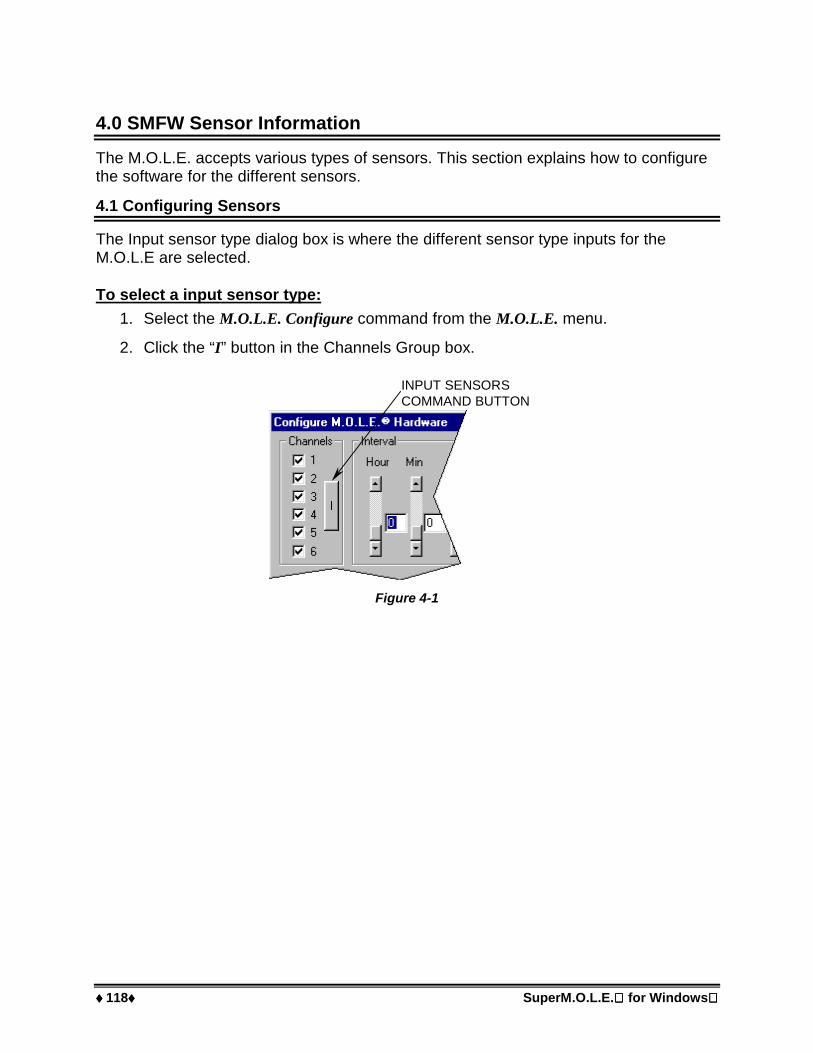
♦♦♦♦ 118♦♦♦♦ SuperM.O.L.E. for Windows
4.0 SMFW Sensor Information
The M.O.L.E. accepts various types of sensors. This section explains how to configurethe software for the different sensors.
4.1 Configuring Sensors
The Input sensor type dialog box is where the different sensor type inputs for theM.O.L.E are selected.
To select a input sensor type:
1. Select the M.O.L.E. Configure command from the M.O.L.E. menu.
2. Click the “I” button in the Channels Group box.
INPUT SENSORSCOMMAND BUTTON
Figure 4-1

SuperM.O.L.E. for Windows ♦♦♦♦ 119♦♦♦♦
3. Select a sensor type. If an Aero or UV sensor is selected the Gain, Offset, orCalibration data can also be entered in the text boxes below the sensor dropdown boxes.
• Click the All Type-K Thermocouples command button to set all channels back totype-K thermocouples.
4. Click the Set command button to make the selected sensor default or the Cancelcommand button to return without saving any changes.
Ony two types of sensors may be selected at one time.
DROP DOWNSENSOR LIST
Figure 4-2: Sensor Configuration Dialog Box
5. When the Set command button is selected, a Scaling dialog box will appear sothe scale can be adjusted to the new sensor(s) configuration.

♦♦♦♦ 120♦♦♦♦ SuperM.O.L.E. for Windows
4.2 Using SMFW with the AeroM.O.L.E. Profiler
SMFW includes several features that are designed to make analysis of Air speedsensor data or a combination of Air speed sensor and thermocouple data easy. (Note,however, that predictions cannot be uses with Air speed data).
To collect data with the Air speed sensor, the software must be configured to thechannels that the Air speed sensor(s) are connected to and their respective calibrationnumber(s). The software will also request unit values for Air speed and scalinginformation.
To configure the software for use with air speed sensors or a combination of Air speedand Thermocouple sensors, refer to section 4.1 Configuring Sensors.
TEMP AXIS UV AXIS
Figure 4-3: Air Profiler Profile
The profile has an additional right Y-axis for Air speed units, and a left Y-axisindicating temperature. If the configuration is only for Air speed, only one axis(left) is used.

SuperM.O.L.E. for Windows ♦♦♦♦ 121♦♦♦♦
4.3 Using SMFW with the UV Sensor
SMFW includes several features that are designed to make analysis of UV sensor dataor a combination of UV sensor and thermocouple data easy. (Note, however, thatpredictions can not be used with UV data).
To collect data from the UV sensor, the software must be configured to the channelsthat the UV Sensor(s) are connected to and their respective calibration number(s). Thesoftware will also request unit values for UV intensity and scaling information.
To configure the software for use with an UV sensor or a combination of an UV andThermocouple sensors, see the information in section 4.1 Configuring Sensors.
To collect UV data, perform a data run with the M.O.L.E. and sensor through a process,then upload the data. After uploading is complete, the UV or combinationUV/Thermocouple profile will appear as below.
TEMP AXIS UV AXIS
Figure 4-4: UV Sensor Profile
The profile has an additional right Y-axis for UV intensity units, and a left Y-axisindicating temperature. If the configuration is only for UV, only one axis (left) isused.

♦♦♦♦ 122♦♦♦♦ SuperM.O.L.E. for Windows
Appendix A: Parameter Definitions
• Value tab
C1, C2, C3, C4 indicate the point, time relative, time absolute, or distance (dependingon the Units setting) on the X axis where the vertical cursors are set, respectively. Thevalues below are the measured values for each channel at that position.
• Time to Reference tab
Low, Medium, and Hi are the temperatures set in the Temp Ref Lines dialog, if set.The values below these are the times in hours, minutes, and seconds (hh:mm:ss) that ittakes for each channel to reach the respective reference value starting from theprocess origin.
• Time Above Reference tab
Values shown in this tab are taken from the graph at it’s present level of magnification.X-axis values outside of view are not included in the calculations. Y-axis values,however are included regardless of magnification level.
Low, Medium, and Hi are the temperatures set in the Temp Ref Lines dialog, if set.The values below these are the times in hours, minutes, and seconds (hh:mm:ss) thateach channel spent at or above the reference value, if at all. All time above thereference values are accumulated in the total no matter where they occur.

SuperM.O.L.E. for Windows ♦♦♦♦ 123♦♦♦♦
Cure Factor%. The cure factor % is based on the time a sensor temperature was abovea temperature reference line divided by the time you entered in the Times Above Temp(TAT) section of the Temp Ref Lines dialog box. This equation gets more complicatedas you add more temperature reference lines. The graph illustrates the times used(shaded area) to sum the total curing time each temperature threshold contributes.
The following equation is used when all three temperature reference lines are used:
Cure Factor % = 100 * ( HItime/HItat + (MEDtime – HItime) /MEDtat + (LOtime – MEDtime)/LOtat )
The same basic equation is used when there are only two (any two) temperaturereference lines used:
Cure Factor % = 100 * ( HItime/HItat + (MEDtime – HItime) /MEDtat )
or
Cure Factor % = 100 * ( MEDtime/MEDtat + (LOtime – MEDtime) /LOtat )
or
Cure Factor % = 100 * ( HItime/HItat + (LOtime – HItime) /LOtat )
Finally, if only one temperature reference line is used, the equation is simply:
Cure Factor % = 100 * time/tat (which ever temp ref line you are using)\
HIref
LOref
MEDref
HI Time
MED Time
LO Time

♦♦♦♦ 1
• Statistics tab:
Values shown in this tab are taken from the graph at it’s present level of magnification.X-axis values outside of view are not included in the calculations. Y-axis values,however are included regardless of magnification level.
Minimum is the lowest value measured. The values below are the minimum values foreach channel.
Minimum X is the point in time where the minimum value occurred. The values beloware the first point on the X-axis where the minimum value occurred for each channel.
Maximum is the highest value measured. The values below are the maximum valuesfor each channel.
Maximum X is the point in time where the maximum value occurred. The values beloware the first point on the X-axis where the maximum value occurred for each channel.
Average is based on the following equation:
Wva
St
Wvadeth
Σx/n
24♦♦♦♦ SuperM.O.L.E. for Windows
here n is the number of data points and x is the value of any given data point. Thelues below are the average values for each channel.
andard Deviation is based on the following equation:
here n is the number of data points and x is the value of any given data point. Thelues below are the standard deviation values for each channel. Small standardviation means the data is used to calculate it is well centered around the average of
at same data.
√(n ⋅ Σx2−(Σx) 2)/n ⋅

SuperM.O.L.E. for Windows ♦♦♦♦ 125♦♦♦♦
• Zone Slopes tab:
Zone 1, Zone 2, Zone3, … are the zones that correspond to the zone parametersentered in the Oven Configure dialog box. Up to 30 zones can be represented. Thevalues below are the slopes within each zone for each channel using the followingequation:
(value at end of zone – value at start of zone)/length of zone in time
Values in bold are the largest values measured for that channel. Slope values are overthe entire zone and cannot reflect transient changes in temperature within a zone.Large zone slopes represent faster heating within a given zone.
Zone1
Zone2
Zone3
Zone4
value at startof zone
value at endof zone
length of zonein time

♦♦♦♦ 126♦♦♦♦ SuperM.O.L.E. for Windows
• Summary Statistics tab
Values shown in this tab are taken from the intire graph regardless of its level ofmagnification.
Peak Temperature is the largest measured value. Values below are the largest valuerecorded for that channel. The higher the peak temperature, the greater the possibilityfor component damage.
Minimum Temperature is the smallest measured value. Values below are the smallestvalue recorded for that channel. Typically, these are the starting values, unless there isactive cooling employed. It is best if starting temperature values are close to the same.This will allow a consistent starting point for other measurements.
Maximum (+) Slope is the largest positive slope measured using a ten point wide (x-axis) differential. Thus, the equation for slope calculation is as follows:
Slope at point X = (Value at point (X + 10) – Value at point X) / (10 * Log interval inseconds)
The values below are the largest positive slope values calculated for each channel. Thelarger the slope, the faster the temperature is increasing (heating).
Time 150°C – 180°C (Time 302°F – 356°F) is the time required for the temperature torise from 150°C (302°F) to 180°C (356°F). The values below are the times in secondsmeasured for each channel. The larger this value, the longer it takes to heat the giventemperature sense point.
Time above 183°C (Time above 361°F) is the total time spent at or above 183°C(361°F) is seconds. This time above may occur anywhere along the x-axis and all willbe accumulated in the total time. Values below are the total times spent at or above foreach channel. The longer the time, the longer typical solder will be in its liquid state.

SuperM.O.L.E. for Windows ♦♦♦♦ 127♦♦♦♦
Maximum (-) Slope is the largest negative slope measured using a ten point wide (x-axis) differential. Thus, the equation for slope calculation is as follows:
Slope at point n = (Value at point (n + 10) – Value at point n) / (10 * Log interval inseconds)
The values below are the largest negative slope values calculated for each channel.The larger the slope, the faster the temperature is falling (cooling).
Range is the difference between the largest and smallest value recorded or calculatedfor each column of data. The smaller the range, the smaller the spread between thevalues collected from each channel.

♦♦♦♦ 128♦♦♦♦ SuperM.O.L.E. for Windows
Appendix B: Pull Down Menus & Toolbar Buttons
The dimmed menu commands are used in other worksheets.
Active menus for the Welcome Worksheet:

SuperM.O.L.E. for Windows ♦♦♦♦ 129♦♦♦♦
Active menus for the Finder Worksheet:

♦♦♦♦ 130♦♦♦♦ SuperM.O.L.E. for Windows
Active menus for the Profile Worksheet:

SuperM.O.L.E. for Windows ♦♦♦♦ 131♦♦♦♦
• SMFW Toolbar Buttons:
3d View New
About Next (Data Run)
Bold Notes
Back (To Previous Data Run) Open
Print Overlay
Align Left Peak Difference
Align Right Prediction
Center Read M.O.L.E. Data
Configure M.O.L.E. Receive RF
Context Help Redo
Copy Save
Erase All Slope
Erase Objects Tolerance Band
First (Data Run) Total Heat
Italic Undo
Last (Data Run) Zoom 100%
Underline Zoom In
Magnify Zoom Out
Measure Zone Matrix