Smart Depth of Field Optimization Applied to a Robotised View Camera

J Math Imaging Vis (2012) 44:1–18DOI 10.1007/s10851-011-0306-y

Smart Depth of Field Optimization Applied to a Robotised ViewCamera

Stéphane Mottelet · Luc de Saint Germain ·Olivier Mondin

Published online: 24 August 2011© Springer Science+Business Media, LLC 2011

Abstract The great flexibility of a view camera allows theacquisition of high quality images that would not be possibleany other way. Bringing a given object into focus is howevera long and tedious task, although the underlying optical lawsare known. A fundamental parameter is the aperture of thelens entrance pupil because it directly affects the depth offield. The smaller the aperture, the larger the depth of field.However a too small aperture destroys the sharpness of theimage because of diffraction on the pupil edges. Hence, thedesired optimal configuration of the camera is such that theobject is in focus with the greatest possible lens aperture. Inthis paper, we show that when the object is a convex poly-hedron, an elegant solution to this problem can be found.It takes the form of a constrained optimization problem, forwhich theoretical and numerical results are given. The opti-mization algorithm has been implemented on the prototypeof a robotised view camera.

Keywords Large format photography · Computationalphotography · Scheimpflug principle

1 Introduction

Since the registration of Theodor Scheimpflug’s patent in1904 (see [6]), and the book of Larmore in 1965 where a

S. Mottelet (�)Laboratoire de Mathématiques Appliquées, Université deTechnologie de Compiègne, 60205 Compiègne, Francee-mail: [email protected]

L. de Saint Germain · O. MondinLuxilon, 21, rue du Calvaire, 92210 Saint-Cloud, France

L. de Saint Germaine-mail: [email protected]

Fig. 1 The Sinar e (a) and its metering back (b)

proof of the so-called Scheimpflug principle can be found(see [3, p. 171–173]), very little has been written about themathematical concepts used in modern view cameras, untilthe development of the Sinar e in 1988 (see Fig. 1). A shortdescription of this camera is given in [7, p. 23]:

The Sinar e features an integrated electronic computer,and in the studio offers a maximum of convenienceand optimum computerized image setting. The user-friendly software guides the photographer through theshot without technical confusion. The photographer

mailto:[email protected]

mailto:[email protected]

2 J Math Imaging Vis (2012) 44:1–18

selects the perspective (camera viewpoint) and thelens, and chooses the areas in the subject that are tobe shown sharp with a probe. From these scatteredpoints the Sinar e calculates the optimum position ofthe plane of focus, the working aperture needed, andinforms the photographer of the settings needed.

Sinar sold a few models of this camera and discontinuedits development in the early nineties. Surprisingly, there hasbeen very little published user feedback about the cameraitself. However many authors started to study (in fact, re-discover) the underlying mathematics (see e.g. [4] and thereferences therein). The most crucial aspect is the consider-ation of depth of field and the mathematical aspects of thisprecise point are now well understood. When the geomet-rical configuration of the view camera is precisely known,then the depth of field region (the region of space where ob-jects have a sharp image) can be determined by using thelaws of geometric optics. Unfortunately, these laws can onlybe used as a rule of thumb when operating by hand on aclassical view camera. Moreover, the photographer is ratherinterested in the inverse problem: given an object whichhas to be rendered sharply, what is the optimal configura-tion of the view camera? A fundamental parameter of thisconfiguration is the aperture of the camera lens. Decreas-ing the lens aperture diameter increases the depth of fieldbut also increases the diffraction of light by the lens en-trance pupil. Since diffraction decreases the sharpness ofthe image, the optimal configuration should be such that theobject fits the depth of field region with the greatest aper-ture.

This paper presents the mathematical tools used in thesoftware of a computer controlled view camera solving thisproblem. Thanks to the high precision machining of its com-ponents, and to the known optical parameters of the lens anddigital sensor, a reliable mathematical model of the viewcamera has been developed. This model allows the acqui-sition of 3D coordinates of the object to be photographed, asexplained in Sect. 2. In Sect. 3 we study the depth of fieldoptimization problem from a theoretical and numerical pointof view. We conclude and briefly describe the architecture ofthe software in Sect. 4.

2 Basic Mathematical Modeling

2.1 Geometrical Model of the View Camera

We consider the robotised view camera depicted in Fig. 2(a)and its geometrical model in Fig. 2(b). We use a global Eu-clidean coordinate system (O,X1,X2,X3) attached to thecamera’s tripod. The front standard, symbolized by its framewith center L of global coordinates L = (L1,L2,L3)

�, canrotate along its tilt and swing axes with angles θL and φL.

Fig. 2 Geometrical model (a) and robotised view camera (b)

Most camera lenses are thick lenses and nodal points H ′and H have to be considered (see [5], pp. 43–46). The rearnodal plane, which is parallel and rigidly fixed to the frontstandard, passes through the rear nodal point H ′. Since L

and H ′ do not necessarily coincide, the translation between

these two points is denoted tL. The vector−−→HH ′ is supposed

to be orthogonal to the rear nodal plane.

J Math Imaging Vis (2012) 44:1–18 3

The rear standard is symbolized by its frame with centerS, whose global coordinates are given by S = (S1, S2, S3)

�.It can rotate along its tilt and swing axes with angles θS andφS . The sensor plane is parallel and rigidly fixed to the rearstandard. The eventual translation between S and the centerof the sensor is denoted by tS.

The rear standard center S can move in the three X1,X2

and X3 directions but the front standard center L is fixed.The rotation matrices associated with the front and rear stan-dard alt-azimuth mounts are respectively given by RL =R(θL,φL) and RS = R(θS,φS) where

R(θ,φ) =⎛⎝

cosφ − sinφ sin θ − sinφ cos θ

0 cos θ − sin θ

sinφ cosφ sin θ cosφ cos θ

⎞⎠ .

The intrinsic parameters of the camera (focal length f , po-sitions of the nodal points H , H ′, translations tS, tL, imagesensor characteristics) are given by their respective manu-facturers data-sheets. The extrinsic parameters of the cam-era are S, L, the global coordinate vectors of S and L, andthe four rotation angles θS , φS , θL, φL. The precise knowl-edge of the extrinsic parameters is possible thanks to thecomputer-aided design model used for manufacturing thecamera components. In addition, translations and rotationsof the rear and front standards are controlled by stepper mo-tors whose positions can be precisely known. In the follow-ing, we will see that this precise geometrical model of theview camera allows one to solve various photographic prob-lems. The first problem is the determination of coordinatesof selected points of the object to be photographed.

In the sequel, for sake of simplicity, we will give all al-gebraic details of the computations for a thin lens, i.e. whenthe two nodal points H , H ′ coincide. In this case, the nodalplanes are coincident in a so-called lens plane. We will alsoconsider that tL = (0,0,0)� so that L is the optical centerof the lens. Finally, we also consider that tS = (0,0,0)� sothat S coincides with the center of the sensor.

2.2 Acquisition of Object Points Coordinates

Let us consider a point X with global coordinates given byX = (X1,X2,X3)

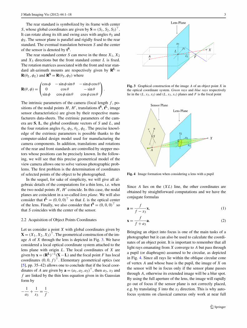
�. The geometrical construction of the im-age A of X through the lens is depicted in Fig. 3. We haveconsidered a local optical coordinate system attached to thelens plane with origin L. The local coordinates of X aregiven by x = (RL)−1(X−L) and the focal point F has localcoordinates (0,0, f )�. Elementary geometrical optics (see[5], pp. 35–42) allows one to conclude that if the local coor-dinates of A are given by a = (a1, a2, a3)

�, then a3, x3 andf are linked by the thin lens equation given in its Gaussianform by

− 1

a3+ 1

x3= 1

f.

Fig. 3 Graphical construction of the image A of an object point X inthe optical coordinate system. Green rays and blue rays respectivelylie in the (L,x3, x2) and (L,x3, x1) planes and F is the focal point

Fig. 4 Image formation when considering a lens with a pupil

Since A lies on the (XL) line, the other coordinates areobtained by straightforward computations and we have theconjugate formulas

a = f

f − x3x, (1)

x = f

f + a3a. (2)

Bringing an object into focus is one of the main tasks of aphotographer but it can also be used to calculate the coordi-nates of an object point. It is important to remember that alllight rays emanating from X converge to A but pass througha pupil (or diaphragm) assumed to be circular, as depictedin Fig. 4. Since all rays lie within the oblique circular coneof vertex A and whose base is the pupil, the image of X onthe sensor will be in focus only if the sensor plane passesthrough A, otherwise its extended image will be a blur spot.By using the full aperture of the lens, the image will rapidlygo out of focus if the sensor plane is not correctly placed,e.g. by translating S into the x3 direction. This is why auto-focus systems on classical cameras only work at near full


aperture: the distance to an object is better determined whenthe depth of field is minimal.

The uncertainty on the position of the sensor plane givingthe best focus is related to the diameter of the so-called “cir-cle of confusion”, i.e. the maximum diameter of a blur spotthat is indistinguishable from a point. Hence, everything de-pends on the size of photosites on the sensor and on the pre-cision of the focusing system (either manual or automatic).This uncertainty is acceptable and should be negligible com-pared to the uncertainty of intrinsic and extrinsic camera pa-rameters.

The previous analysis shows that the global coordinatesof X can be computed, given the position (u, v)� of its im-age A on the sensor plane. This idea has been already usedon the Sinar e, where the acquisition of (u, v)� was done byusing a mechanical metering unit (see Fig. 1 (b)). In the sys-tem we have developed, a mouse click in the live video win-dow of the sensor is enough to indicate these coordinates.Once (u, v)� is known, the coordinates of A in the globalcoordinate system are given by

A = S + RS

⎛⎝

u

v

0

⎞⎠ ,

and its coordinates in the optical system by

a = (RL)−1(A − L).

Then the local coordinate vector x of the reciprocal imageis computed with (2) and the global coordinate vector X isobtained by

X = L + RLx.

By iteratively focusing on different parts of the object, thephotographer can obtain a set of points X = {X1, . . . ,Xn},with n ≥ 3, which can be used to determine the best configu-ration of the view camera, i.e. the positions of front and rearstandards and their two rotations, in order to satisfy focusrequirements.

3 Focus and Depth of Field Optimization

In classical digital single-lens reflex (DSLR) cameras, thesensor plane is always parallel to the lens plane and to theplane of focus. For example, bringing into focus a long andflat object which is not parallel to the sensor needs to de-crease the aperture of the lens in order to extend the depthof field. On the contrary, view cameras with tilts and swings(or DSLR with a tilt/shift lens) allow to skew away the planeof focus from the parallel in any direction. Hence, bringinginto focus the same long and flat object with a view camera

can be done at full aperture. This focusing process is unfor-tunately very tedious. However, if a geometric model of thecamera and the object are available, the adequate rotationscan be estimated precisely. In the next sections, we will ex-plain how to compute the rear standard position and the tiltand swing angles of both standards to solve two differentproblems:

1. When the focus zone is roughly flat, and depth of fieldis not a critical issue, then the object plane is computedfrom the set of object points X . If n = 3 and the pointsare not collinear then this plane is uniquely defined. Ifn > 3 and at least 3 points are not collinear, we computethe best fitting plane minimizing the sum of squared or-thogonal distances to points of X . Then, we are able tobring this plane into sharp focus by acting on:(a) the angles θL and φL of the front standard and the

position of the rear standard, for arbitrary rotationangles θS , φS .

(b) the angles θS , φS and position of the rear standard,for arbitrary rotation angles θL, φL (in this case thereis a perspective distortion).

2. When the focus zone is not flat, then the tridimensionalshape of the object has to be taken into account.

The computations in case 1 are detailed in Sect. 3.1. InSect. 3.3 a general algorithm is described that allows thecomputation of angles θL and φL of the front standard andthe position of the rear standard such that all the objectpoints are in the depth of field region with a maximum aper-ture. We give a theoretical result showing that the determi-nation of the solution amounts to enumerate a finite numberof configurations.

3.1 Placement of the Plane of Sharp Focus by Using Tiltand Swing Angles

In this section we study the problem of computing the tiltand swing angles of front standard and the position of therear standard for a given sharp focus plane. Although theunderlying laws are well-known and are widely described(see [2, 4, 8]), the detail of the computations is always donefor the particular case where only the tilt angle θ is consid-ered. Since we aim to consider the more general case wheretilt and swing angles are used, we will describe the variousobjects (lines, planes) and the associated computations byusing linear algebra tools.

3.1.1 The Scheimpflug and the Hinge Rules

In order to explain the Scheimpflug rule, we will refer tothe diagram depicted in Fig. 5. The Plane of sharp focus(abbreviated SFP) is determined by a normal vector nSF anda point Y . The position of the optical center L and a vector


Fig. 5 Illustration of the Scheimpflug rule

Fig. 6 Illustration of the hinge rule

nS normal to the sensor plane (abbreviated SP) are known.The unknowns are the position of the sensor center S and avector nL normal to the lens plane (abbreviated LP).

The Scheimpflug rule stipulates that if SFP is into focus,then SP, LP and SFP necessarily intersect on a common linecalled the “Scheimpflug Line” (abbreviated SL). The dia-gram of Fig. 5 should help the reader to see that this rule isnot sufficient to uniquely determine nL and SP, as this planecan be translated toward nS if nL is changed accordingly.

The missing constraints are provided by the hinge rule,which is illustrated in Fig. 6. This rule considers two com-plimentary planes: the front focal plane (abbreviated FFP),which is parallel to LP and passes through the focal point F ,and the parallel to sensor lens plane (abbreviated PSLP),which is parallel to SP and passes through the optical cen-

ter L. The hinge rule stipulates that FFP, PSLP and SFPmust intersect along a common line called the hinge Line(abbreviated HL). Since HL is uniquely determined as theintersection of SFP and PSLP, this allows one to determinenL, or equivalently the tilt and swing angles, such that FFPpasses through HL and F . Then SL is uniquely defined asthe intersection of LP and SFP by the Scheimpflug rule(note that SL and HL are parallel by construction). SincenS is already known, any point belonging to SL is sufficientto uniquely define SP. Hence, the determination of tilt andswing angles and position of the rear standard can be sum-marized as follows:

1. determination of HL, intersection of FFP and SFP,2. determination of tilt and swing angles such that HL be-

longs to FFP,3. determination of SL, intersection of LP and SFP,4. translation of S such that SL belongs to SP.

3.1.2 Algebraic Details of the Computations

In this section the origin of the coordinate system is the op-tical center L and the inner product of two vectors X and Yis expressed by using the matrix notation X�Y. All planesare defined by a unit normal vector and a point in the planeas follows:

SP ={

X ∈ R3, (X − S)�nS = 0

}

PSLP ={

X ∈ R3, X�nS = 0

},

LP ={

X ∈ R3, X�nL = 0

},

FFP ={

X ∈ R3, X�nL − f = 0

},

SFP ={

X ∈ R3, (X − Y)�nSF = 0

},

where the equation of FFP takes this particular form becausethe distance between L and F is equal to the focal length f

and we have imposed that nL3 > 0. The computations are

detailed in the following algorithm:

Algorithm 1

Step 1: compute the hinge line by considering its parametricequation

HL ={

X ∈ R3,∃t ∈ R,X = W + tV

},

where V is a direction vector and W is the coordinatevector of an arbitrary point of HL. Since this line is theintersection of PSLP and SFP, V is orthogonal to nS andnSF. Hence, we can take V as the cross product

V = nSF × nS


and W as a particular solution (e.g. the solution of mini-mum norm) of the overdetermined system of equations

W�nS = 0,

W�nSF = Y�nSF.

Step 2: since HL belongs to FFP we have

(W + tV)�nL − f = 0, ∀ t ∈ R,

hence nL verifies the overdetermined system of equations

W�nL = f, (3)

V�nL = 0. (4)

with the constraint ‖nL‖2 = 1. The computation of nL canbe done by the following two steps:

1. compute W = V × W and V the minimum norm solu-tion of system (3)–(4), which gives a parametrization

nL = V + tW,

of all its solutions, where t is an arbitrary real.2. determination of t such that ‖nL‖2 = 1: this is done by

taking the solution t of the second degree equation

W�Wt2 + 2W�Vt + V�V − 1 = 0,

such that nL3 > 0. The tilt and swing angles are then

obtained as

θL = − arcsinnL2 , φL = − arcsin

nL1

cos θL

.

Step 3: since SL is the intersection of LP and SFP, the coor-dinate vector U of a particular point U on SL is obtainedas the minimum norm solution of the system

U�nL = 0,

U�nSF = W�nSF,

where we have used the fact that W ∈ SFP.Step 4: the translation of S can be computed such that U

belongs to SP, i.e.

(U − S)�nS = 0.

If we only act on the third coordinate of S and leave thetwo others unchanged, then S3 can be computed as

S3 = U�nS − S1nS1 − S2n

S2

nS3

.

Fig. 7 Position of planes SFP1 and SFP2 delimiting the depth of fieldregion

Remark 1 When we consider a true camera lens, the nodalpoints H,H ′ and the front standard center L do not coin-cide. Hence, the tilt and swing rotations of the front standardmodify the actual position of the PSLP plane. In this case,we use the following iterative fixed point scheme:

1. The angles φL and θL are initialized with starting valuesφ0

L and θ0L.

2. At iteration k,(a) the position of PSLP is computed considering φk

L

and θkL,

(b) the resulting hinge Line is computed, then the posi-tion of FFP and the new values φk+1

L and θk+1L are

computed.

Point 2 is repeated until convergence of φkL and θk

L up to agiven tolerance. Generally 3 iterations are sufficient to reachthe machine precision.

3.2 Characterization of the Depth of Field Region

As in the previous section, we consider that L and the nodalpoints H and H ′ coincide. Moreover, L will be the origin ofthe global coordinates system.

We consider the configuration depicted in Fig. 7 wherethe sharp focus plane SFP, the lens plane LP and the sensorplane SP are tied by the Scheimpflug and the hinge rule. Thedepth of field can be defined as follows:

Definition 1 Let X be a 3D point and A its image throughthe lens. Let C be the disk in LP of center L and diameterf/N , where N is called the f-number. Let K be the coneof base C and vertex A. The point X is said to lie in thedepth of field region if the diameter of the intersection of SP


and K is lower that c, the diameter of the so-called circle ofconfusion.

The common values of c, which depend on the magnifica-tion from the sensor image to the final image and on its view-ing conditions, lie typically between 0.2 mm and 0.01 mm.In the following the value of c is not a degree of freedom buta given input.

If the ellipticity of extended images is neglected, thedepth of field region can be shown to be equal to the un-bounded wedge delimited by SFP1 and SFP2 intersecting atHL. The corresponding sensor planes SP1 and SP2 are tiedto SFP1 and SFP2 by the Scheimpflug rule. By mentally ro-tating SFP around HL, it is easy to see that SP is translatedthrough nS and spans the region between SP1 and SP2. Theposition of SP1 and SP2, the f-number N and the diameterof the circle of confusion c are related by the formula

Nc

f= p1 − p2

p1 + p2, (5)

where p1, respectively p2, are the distances between the op-tical center L and SP1, respectively SP2, both measured or-thogonally to the optical plane. The distance p between SPand L can be shown to be equal to

p = 2p1p2

p1 + p2, (6)

the harmonic mean of p1 and p2. This approximate defini-tion of the depth of field region has been proposed by vari-ous authors (see [1, 8]) but when the ellipticity of images istaken into account a complete study can be found in [2]. Forsake of completeness, we give the justification of formulas(5) and (6) in Appendix A.1. In most practical situations thenecessary angle between SP and LP is small (less that 10degrees), so that this approximation is correct.

Remark 2 The analysis in Appendix A.1 shows that the ratioNcf

in (5) does not depend on the direction used for measur-ing the distance between SP, SP1, SP2 and L. The only con-dition, in order to take into account the case where SP andLP are parallel, is that this direction is not orthogonal to nS.Hence, by taking the direction given by nS, we can obtainan equivalent formula to (5). To compute the distances, weneed the coordinate vector of two points U1 and U2 on SP1

and SP2 respectively. To this purpose we consider Step 3 ofAlgorithm 1 in Sect. 3.1: if W is the coordinate vector ofany point W of HL, each vector Ui can be obtained as aparticular solution of the system

Ui�nL = 0,

Ui�ni = W�ni .

Since SPi can be defined as

SPi ={

X ∈ R3, (X − Ui )

�nS = 0

},

and ‖nS‖ = 1, the signed distance from L to SPi is equal to

d(L,SPi) = Ui�nS.

So the equivalent formula giving the ratio Ncf

is given by

Nc

f=

∣∣∣∣d(L,SP1) − d(L,SP2)

d(L,SP1) + d(L,SP2)

∣∣∣∣

=∣∣∣∣(U1 − U2)

�nS

(U1 + U2)�nS

∣∣∣∣. (7)

The above considerations show that for a given orienta-tion of the rear standard given by nS, if the depth of fieldwedge is given, then the needed f-number, the tilt and swingangles of the front standard and the translation of the sen-sor plane, can be determined. The related question that willbe addressed in the following is the question: given a setof points X = {X1, . . . ,Xn}, how can we minimize the f-number such that all points of X lie in the depth of fieldregion?

3.3 Depth of Field Optimization with Respect to Tilt Angle

We first study the depth of field optimization in two dimen-sions, because in this particular case all computations can becarried explicitly and a closed form expression is obtained,giving the f-number as a function of front standard tilt angleand of the slope of limiting planes. First, notice that N has anatural upper bound, since (5) implies that

N ≤ f

c.

3.3.1 Computation of f -Number with Respect to Tilt Angleand Limiting Planes

Without loss of generality, we consider that the sensor planehas the normal nS = (0,0,1)�. Let us denote by θ the tiltangle of the front standard and consider that the swing angleφ is zero. The lens plane is given by

LP ={

X ∈ R3, X�nL = 0

},

where

nL = (0,− sin θ, cos θ)�,

and any collinear vector to nL × nS is a direction vector ofthe hinge Line. Hence we can take, independently of θ ,

V = (1,0,0)�


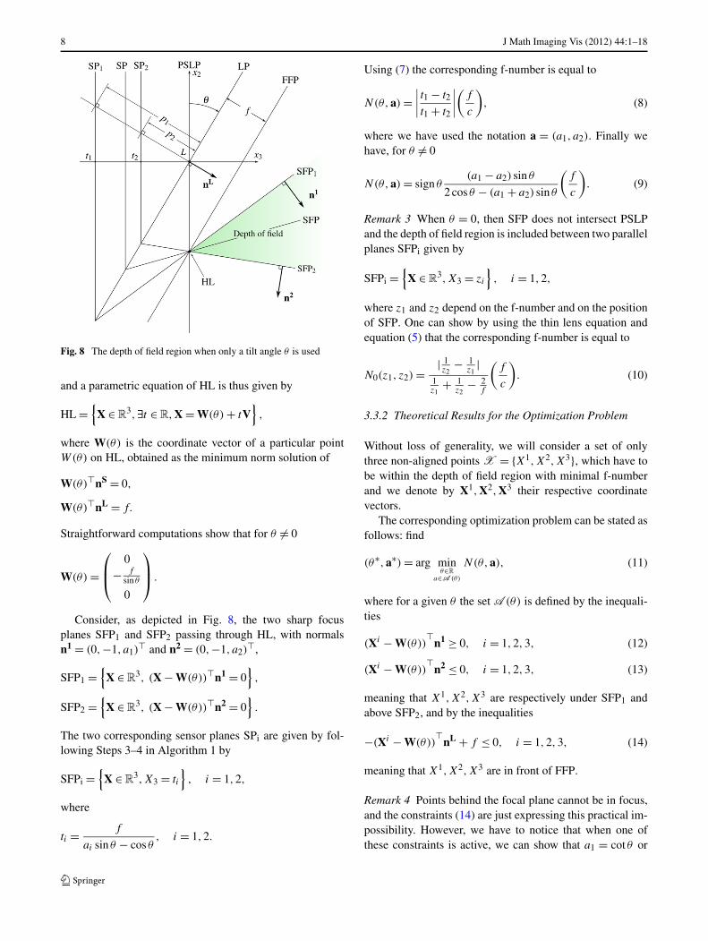
Fig. 8 The depth of field region when only a tilt angle θ is used

and a parametric equation of HL is thus given by

HL ={

X ∈ R3,∃t ∈ R,X = W(θ) + tV

},

where W(θ) is the coordinate vector of a particular pointW(θ) on HL, obtained as the minimum norm solution of

W(θ)�nS = 0,

W(θ)�nL = f.

Straightforward computations show that for θ �= 0

W(θ) =⎛⎜⎝

0− f

sin θ

0

⎞⎟⎠ .

Consider, as depicted in Fig. 8, the two sharp focusplanes SFP1 and SFP2 passing through HL, with normalsn1 = (0,−1, a1)

� and n2 = (0,−1, a2)�,

SFP1 ={

X ∈ R3, (X − W(θ))�n1 = 0

},

SFP2 ={

X ∈ R3, (X − W(θ))�n2 = 0

}.

The two corresponding sensor planes SPi are given by fol-lowing Steps 3–4 in Algorithm 1 by

SFPi ={

X ∈ R3,X3 = ti

}, i = 1,2,

where

ti = f

ai sin θ − cos θ, i = 1,2.

Using (7) the corresponding f-number is equal to

N(θ,a) =∣∣∣∣t1 − t2

t1 + t2

∣∣∣∣(

f

c

), (8)

where we have used the notation a = (a1, a2). Finally wehave, for θ �= 0

N(θ,a) = sign θ(a1 − a2) sin θ

2 cos θ − (a1 + a2) sin θ

(f

c

). (9)

Remark 3 When θ = 0, then SFP does not intersect PSLPand the depth of field region is included between two parallelplanes SFPi given by

SFPi ={

X ∈ R3,X3 = zi

}, i = 1,2,

where z1 and z2 depend on the f-number and on the positionof SFP. One can show by using the thin lens equation andequation (5) that the corresponding f-number is equal to

N0(z1, z2) = | 1z2

− 1z1

|1z1

+ 1z2

− 2f

(f

c

). (10)

3.3.2 Theoretical Results for the Optimization Problem

Without loss of generality, we will consider a set of onlythree non-aligned points X = {X1,X2,X3}, which have tobe within the depth of field region with minimal f-numberand we denote by X1,X2,X3 their respective coordinatevectors.

The corresponding optimization problem can be stated asfollows: find

(θ∗,a∗) = arg minθ∈R

a∈A (θ)

N(θ,a), (11)

where for a given θ the set A (θ) is defined by the inequali-ties

(Xi − W(θ))�

n1 ≥ 0, i = 1,2,3, (12)

(Xi − W(θ))�

n2 ≤ 0, i = 1,2,3, (13)

meaning that X1,X2,X3 are respectively under SFP1 andabove SFP2, and by the inequalities

−(Xi − W(θ))�

nL + f ≤ 0, i = 1,2,3, (14)

meaning that X1,X2,X3 are in front of FFP.

Remark 4 Points behind the focal plane cannot be in focus,and the constraints (14) are just expressing this practical im-possibility. However, we have to notice that when one ofthese constraints is active, we can show that a1 = cot θ or


a2 = cot θ so that N(a, θ) reaches its upper bound fc

. More-over, we have to eliminate the degenerate case where thepoints Xi are such that there exists two active constraints in(14): in this case, there exists a unique admissible pair (a, θ)

and the problem has no practical interest. To this purpose,we can suppose that Xi

3 > f for i = 1,2,3.

For θ �= 0 the gradient of N(a, θ) is equal to

∇(a, θ) = 2 sign θ

(2 cot θ − (a1 + a2))2

⎛⎜⎜⎝

cot θ − a2

− cot θ + a1

a1−a2sin2 θ

⎞⎟⎟⎠

and cannot vanish since a1 = a2 is not possible becauseit would mean that X1,X2,X3 are collinear. This impliesthat a lies on the boundary of A (θ) and we have the follow-ing intuitive result (the proof is given in Appendix A.2):

Proposition 1 Suppose that Xi3 > f , for i = 1,2,3. Then

when N(a, θ) reaches its minimum, there exists i1, i2 withi1 �= i2 such that

(Xi1 − W(θ))�

n1 = 0,

(Xi2 − W(θ))�

n2 = 0.

Remark 5 The above result shows that at least two pointstouch the depth of field limiting planes SFP1 and SFP2 whenthe f-number is minimal. In the following, we will show thatthe three points X1,X2 and X3 are necessarily in contactwith one of the limiting planes (the proof is given in Ap-pendix A.3):

Proposition 2 Suppose that the vertices {Xi}i=1...3 verifythe condition

‖Xi × Xj‖‖Xi − Xj‖ > f, i �= j. (15)

Then N(a, θ) reaches its minimum when all vertices are incontact with the limiting planes.

Remark 6 If θ is small, then N(θ,a) in (9) can be approxi-mated by

N(θ,a) = sign θ(a1 − a2) sin θ

(f

2c

), (16)

and the proof of Proposition 2 is considerably simplified: thesame result holds with the weaker condition

‖Xi × Xj‖ > 0. (17)

In fact, an approximate way of specifying the depth of fieldregion using the hyperfocal distance, proposed in [4], leads

to the same approximation of N(θ,a), under the a priorihypothesis of small θ and distant objects, i.e. Xi

3 � f . Thisremark is clarified in Appendix A.4.

We will illustrate the theoretical result by considering setsof 3 points. For a set with more than 3 vertices (but beingequal to the vertices of the convex hull of X ), the determi-nation of the optimal solution is purely combinatorial, sinceit is enough to enumerate all admissible situations where twopoints are in contact with one plane, and a third one with theother. The value θ = 0 also has to be considered because itcan be a critical value if the object has a vertical edge. Wewill also give an Example which violates condition (15) andwhere N(a, θ) reaches its minimum when only two verticesare in contact with the limiting planes.

3.3.3 Numerical Results

In this section, we will consider the following function, de-fined for θ �= 0

n(θ) = mina∈A (θ)

N(a, θ).

Finding the minimum of this function allows one to solve theoriginal constrained optimization problem, but consideringthe results of the previous section, n(θ) is non-differentiable.In fact, the values of θ for which n(θ) is not differentiablecorrespond to the situations where 3 points are in contactwith the limiting planes. We extend n(θ) by continuity forθ = 0 by defining

n(0) =1z2

− 1z1

1z1

+ 1z2

− 2f

(f

c

),

where

z1 = maxi=1,2,3

Xi3, z2 = min

i=1,2,3Xi

3.

This formula can be directly obtained by using conjugationformulas or by taking θ = 0 in (24) in Appendix A.3.

Example 1 We consider a lens with focal length f = 5 ×10−2 m and a confusion circle c = 3 × 10−5 m (commonlyused value for 24 × 36 cameras). The vertices have coordi-nates

X1 =⎛⎝

0−11

⎞⎠ , X2 =

⎛⎝

031

⎞⎠ , X3 =

⎛⎝

00

1.5

⎞⎠ .

Figure 9 shows the desired depth of field region (dashedzone) and the three candidates hinge lines corresponding tocontacts EijVk :


Fig. 9 Enumeration of the 3 candidates configurations for Example 1

Table 1 Value of θ for eachpossible optimal contact andcorresponding f-number n(θ)

for Example 1

Contact θ n(θ)

E12V3 0.0166674 9.52

E13V2 0.025002 7.16

E23V1 0.0500209 28.28

• E12V3, obtained when the edge [X1,X2] is in contactwith SFP1 and vertex X3 with SFP2.



The associated values of θ and n(θ) are given in Table 1,which shows that contact E13V2 seems to give the minimumf-number. Condition (15) is verified, since

‖X1 × X2‖‖X1 − X2‖ = 1,

‖X1 × X3‖‖X1 − X3‖ = 1.34,

‖X2 × X3‖‖X2 − X3‖ = 1.48.

Hence, the derivative of n(θ) cannot vanish and the mini-mum f-number is necessarily reached for θ∗ = 0.025002.

We can confirm this by considering the graph of n(θ)

depicted on Fig. 10. In the zone of interest, the functionn(θ) is almost piecewise affine. For each point in the in-terior of curved segments of the graph, the value of θ is suchthat the contact of X with the limiting planes is of typeViVj . Clearly, the derivative of n(θ) does not vanish. Thepossible optimal values of θ , corresponding to contacts of

Fig. 10 Example 1 graph of n(θ) for θ ∈ [−0.6,0.6] (a) andθ ∈ [0,0.06] (b). Labels give the different types of contact.

Table 2 Value of θ for eachpossible optimal contact andcorresponding f-number n(θ)

for Example 2

Contact θ n(θ)

E12V3 0.185269 29.49

E23V1 0.100419 83.67

E13V2 0.235825 47.04

type EijVk , are the abscissa of angular points of the graph,marked with red dots. The graph confirms that the minimalvalue of n(θ) is reached for contact E12V3.

The minimal f-number is equal to n(θ∗) = 7.16. By com-parison, the f-number without tilt optimization is n(0) =28.74. This example highlights the important gain in termsof f-number reduction with the optimized tilt angle.

Example 2 We consider the same lens and confusion circleas in Example 1 (f = 5.10−2 m, c = 3.10−5 m) but the ver-tices have coordinates

X1 =⎛⎝

0−0.10.12

⎞⎠ , X2 =

⎛⎝

00

0.19

⎞⎠ ,


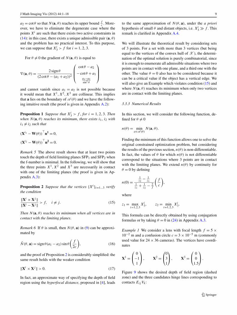
Fig. 11 Example 2 graph of n(θ) for θ ∈ [−0.6,0.6] (a) andθ ∈ [0,0.3] (b). Labels give the different types of contact

X3 =⎛⎝

0−0.0525

0.17

⎞⎠ .

The object is almost ten times smaller than the object of theprevious example (it has the size of a small pen), but it is alsoten times closer: this is a typical close up configuration. Thevalues of θ and n(θ) associated to contacts of type EijVk

are given in Table 2 which shows that contact E13V2 seemsto give the minimum f-number. We have

‖X1 × X2‖‖X1 − X2‖ = 0.16,

‖X1 × X3‖‖X1 − X3‖ = 0.16,

‖X2 × X3‖‖X2 − X3‖ = 0.1775527,

showing that condition (15) is still verified, even if the val-ues are smaller than the values of Example 1. Hence, thederivative of n(θ) cannot vanish and the minimum f-numberis reached for θ∗ = 0.185269.

We can confirm this by considering the graph of n(θ) de-picted on Fig. 11. As in Example 1, the derivative of n(θ)

does not vanish and the graph confirms that the minimalvalue of n(θ) is reached for contact E12V3.

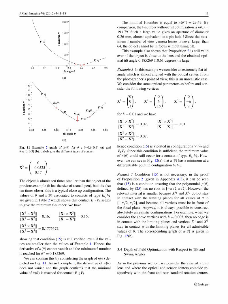
The minimal f-number is equal to n(θ∗) = 29.49. Bycomparison, the f-number without tilt optimization is n(0) =193.79. Such a large value gives an aperture of diameter0.26 mm, almost equivalent to a pin hole ! Since the max-imum f-number of view camera lenses is never larger than64, the object cannot be in focus without using tilt.

This example also shows that Proposition 2 is still valideven if the object is close to the lens and the obtained opti-mal tilt angle 0.185269 (10.61 degrees) is large.

Example 3 In this example we consider an extremely flat tri-angle which is almost aligned with the optical center. Fromthe photographer’s point of view, this is an unrealistic case.We consider the same optical parameters as before and con-sider the following vertices

X1 =⎛⎝

001

⎞⎠ , X2 =

⎛⎝

0h

1.5

⎞⎠ , X3 =

⎛⎝

0−h

2

⎞⎠ ,

for h = 0.01 and we have

‖X1 × X2‖‖X1 − X2‖ = 0.02,

‖X1 × X3‖‖X1 − X3‖ = 0.01,

‖X2 × X3‖‖X2 − X3‖ = 0.07,

hence condition (15) is violated in configurations V1V2 andV1V3. Since this condition is sufficient, the minimum valueof n(θ) could still occur for a contact of type EijVk . How-ever, we can see in Fig. 12(a) that n(θ) has a minimum at adifferentiable point in configuration V1V3.

Remark 7 Condition (15) is not necessary: in the proofof Proposition 2 (given in Appendix A.3), it can be seenthat (15) is a condition ensuring that the polynomial p(θ)

defined by (25) has no root in [−π/2,π/2]. However, therelevant interval is smaller because Xi1 and Xi2 do not stayin contact with the limiting planes for all values of θ in[−π/2,π/2], and because all vertices must be in front ofthe focal plane. Anyway, it is always possible to constructabsolutely unrealistic configurations. For example, when weconsider the above vertices with h = 0.005, then no edge isin contact with the limiting planes and vertices X1 and X3

stay in contact with the limiting planes for all admissiblevalues of θ . The corresponding graph of n(θ) is given inFig. 12(b).

3.4 Depth of Field Optimization with Respect to Tilt andSwing Angles

As in the previous section, we consider the case of a thinlens and where the optical and sensor centers coincide re-spectively with the front and rear standard rotation centers.


Fig. 12 Example 3 graphs of n(θ) for θ ∈ [−1,1]

Without loss of generality, we consider that the sensor planehas the normal nS = (0,0,1)�. The lens plane is given by

LP ={

X ∈ R3, X�nL = 0

},

where

nL = (− sinφ cos θ,− sin θ, cosφ cos θ)�.

A parametric equation of HL is given by

HL ={

X ∈ R3,∃t ∈ R,X = W(θ,φ) + tV(θ,φ)

},

where the direction vector is given by

V(θ,φ) = nL × nS = (− sin θ, sinφ cos θ,0)�,

and W(θ,φ) is the coordinate vector of a particular pointW(θ,φ) on HL, obtained as the minimum norm solution of

W(θ,φ)�nS = 0,

W(θ,φ)�nL = f.

Consider, as depicted in Fig. 7, the two planes of sharp fo-cus SFP1 and SFP2 intersecting at HL, with normals n1

and n1 respectively. The point W(θ,φ) belongs to SFP1 and

Fig. 13 Position of the hinge line when both tilt and swing are usedand nS = (0,0,1)�. The LP and FFP planes have not been representedfor reasons of readability

SFP2 and any direction vector of SFP1 ∩ SFP2 is collinearto V(θ,φ). Hence, we have

SFP1 ={

X ∈ R3, (X − W(θ,φ))�n1 = 0

},

SFP2 ={

X ∈ R3, (X − W(θ,φ))�n2 = 0

},

and

(n1 × n2) × V(θ,φ) = 0. (18)

Using (7) the f-number is equal to

N(θ,φ,n1,n2) = f

c

∣∣∣∣(U1 − U2)

�nS

(U1 + U2)�nS

∣∣∣∣, (19)

where each coordinate vector Ui of point Ui , for i = 1,2, isobtained as a particular solution of the following system:

Ui�nL = 0,

Ui�ni = W(θ,φ)�ni .

Remark 8 When nS = (0,0,1)� the intersections of HLwith the (L,X1) and the (L,X2) axes can be determined,as depicted in Fig. 13. In this case, it is easy to show that thecoordinates of the minimum norm W(θ,φ) are given by

W(θ,φ) = − f

sin2 φ cos2 θ + sin2 θ(sinφ cos θ, sin θ,0)�.


We note that up to a rotation of axis (0,0,1)� and angle α,we recover a configuration where only a tilt angle ψ is used,where these two angles are respectively defined by

sinψ = sign θ

√sin2 φ cos2 θ + sin2 θ,

sinα = sinφ cos θ

sinψ.

3.4.1 Optimization Problem

Consider a set 4 non coplanar points X = {Xi}i=1...4, whichhave to be within the depth of field region with minimal f-number and denote by {Xi}i=1...4 their respective coordinatevectors. The optimization problem can be stated as follows:find

(θ∗, φ∗,n1∗,n2∗

) = arg minθ,φ,n1,n2

N(θ,φ,n1,n2), (20)

where the minimum is taken for θ,φ,n1 and n2 such that(18) is verified and such that the points {Xi}i=1...4 lie be-tween SFP1 and SFP2. This last set of constraints can beexpressed in a way similar to (12)–(13).

3.4.2 Analysis of Configurations

Consider the function n(θ,φ) defined by

n(θ,φ) = minn1,n2

N(θ,φ,n1,n2), (21)

where n1 and n2 are constrained as in the previous section.Consider the two limiting planes SFP1 and SFP2 with nor-mals n1 and n2 satisfying the minimum in (21). Using therotation argument of Remark 8 we can easily show that SFP1

and SFP2 are necessary in contact with at least two vertices.However, for each value of the pair (θ,φ), we have threetypes of possible contact between the tetrahedron formedby points {Xi}i=1...4 and the limiting planes: vertex-vertex,edge-vertex, edge-edge or face-vertex. These configurationscan be analyzed as follows: let us consider a pair (θ0, φ0)

and the corresponding type of contact:

Vertex-vertex: each limiting plane is in contact with onlyone vertex, respectively Vi and Vj . In this case, n(θ,φ) isdifferentiable at (θ0, φ0) and there exists a curve γvv de-fined by

γvv(t) = (θ(t), φ(t)), γvv(0) = (θ0, φ0),

such that ddt

n(θ(t), φ(t)) exists and does not vanish fort = 0. This can be proved using again the rotation argu-ment of Remark 8. Hence, n(θ0, φ0) cannot be minimal.

Table 3 Value of θ and φ for each possible optimal contact and corre-sponding f-number n(θ,φ)

Contact θ φ n(θ,φ)

E12E34 0.021430 −0.028582 12.35

E23E14 0.150568 −0.203694 90.75

E13E24 0.030005 −0.020010 8.64

F123V4 0 0.100167 88.18

F243V1 0.075070 −0.050162 42.91

F134V2 0.033340 −0.033358 9.64

F124V3 0.018751 −0.012503 10.76

Edge-vertex: one of the two planes is in contact with edgeEij and the other one is in contact with vertex Vk . In thiscase there is still a degree of freedom since the plane incontact with Eij can rotate around this edge in either di-rections while keeping the other plane in contact with Vk

only. If the plane in contact with Eij is SFP1, its normal n1

can be parameterized by using a single scalar parameter t

and we obtain a family of planes defined by

SFP1(t) ={

X ∈ R3,n1(t)

�(X − Xi ) = 0

}.

For each value of t , the intersection of SFP1(t) with PSLPdefines a hinge Line and thus a pair (θ(t), φ(t)) of tilt andswing angles. Hence, there exists a parametric curve

γev(t) = (θ(t), φ(t)), γev(0) = (θ0, φ0), (22)

along which n(θ,φ) is differentiable. As we will see in thenumerical results, the curve γev(t) is almost a straight linewhen θ and φ are small, and d

dtn(θ,φ(t)) does not vanish

for t = 0.Edge-edge: the limiting planes are respectively in con-

tact with edges Eij , Ekl connecting, respectively, verticesVi,Vj and vertices Vk,Vl . There is no degree of free-dom left since these edges cannot be parallel (otherwiseall points would be coplanar). Hence, n(θ,φ) is not differ-entiable at (θ0, φ0).

Face-vertex: the limiting planes are respectively in contactwith vertex Vl and with the face Fijk connecting verticesVi,Vj ,Vk . As in the previous case, there is no degree offreedom left and n(θ,φ) is not differentiable at (θ0, φ0).

We can already speculate that the first two configura-tions are necessary suboptimal. Consequently we just haveto compute the f-number associated with each one of the 7possible configurations of type edge-edge of face-vertex.

3.4.3 Numerical Results

We have considered the flat object of Example 1, translatedin plane X1 = −0.5, and a complimentary point in order to


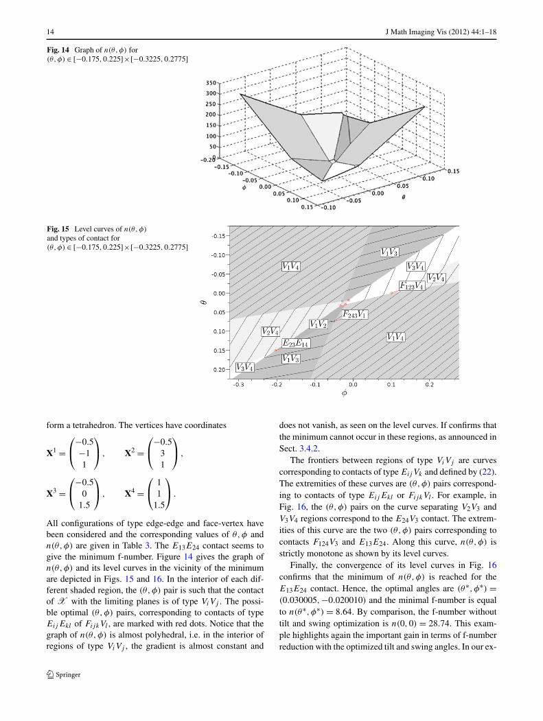
Fig. 14 Graph of n(θ,φ) for(θ,φ) ∈ [−0.175,0.225]×[−0.3225,0.2775]

Fig. 15 Level curves of n(θ,φ)

and types of contact for(θ,φ) ∈ [−0.175,0.225]×[−0.3225,0.2775]

form a tetrahedron. The vertices have coordinates

X1 =⎛⎝

−0.5−11

⎞⎠ , X2 =

⎛⎝

−0.531

⎞⎠ ,

X3 =⎛⎝

−0.50

1.5

⎞⎠ , X4 =

⎛⎝

11

1.5

⎞⎠ .

All configurations of type edge-edge and face-vertex havebeen considered and the corresponding values of θ,φ andn(θ,φ) are given in Table 3. The E13E24 contact seems togive the minimum f-number. Figure 14 gives the graph ofn(θ,φ) and its level curves in the vicinity of the minimumare depicted in Figs. 15 and 16. In the interior of each dif-ferent shaded region, the (θ,φ) pair is such that the contactof X with the limiting planes is of type ViVj . The possi-ble optimal (θ,φ) pairs, corresponding to contacts of typeEijEkl of FijkVl , are marked with red dots. Notice that thegraph of n(θ,φ) is almost polyhedral, i.e. in the interior ofregions of type ViVj , the gradient is almost constant and

does not vanish, as seen on the level curves. If confirms thatthe minimum cannot occur in these regions, as announced inSect. 3.4.2.

The frontiers between regions of type ViVj are curvescorresponding to contacts of type EijVk and defined by (22).The extremities of these curves are (θ,φ) pairs correspond-ing to contacts of type EijEkl or FijkVl . For example, inFig. 16, the (θ,φ) pairs on the curve separating V2V3 andV3V4 regions correspond to the E24V3 contact. The extrem-ities of this curve are the two (θ,φ) pairs corresponding tocontacts F124V3 and E13E24. Along this curve, n(θ,φ) isstrictly monotone as shown by its level curves.

Finally, the convergence of its level curves in Fig. 16confirms that the minimum of n(θ,φ) is reached for theE13E24 contact. Hence, the optimal angles are (θ∗, φ∗) =(0.030005,−0.020010) and the minimal f-number is equalto n(θ∗, φ∗) = 8.64. By comparison, the f-number withouttilt and swing optimization is n(0,0) = 28.74. This exam-ple highlights again the important gain in terms of f-numberreduction with the optimized tilt and swing angles. In our ex-


Fig. 16 Level curves of n(θ,φ)

and types of contact for(θ,φ) ∈ [−0.015,0.035]×[−0.0375,−0.0075]

perience, the optimal configuration for general polyhedronscan be of type edge-edge or face-vertex.

4 Trends and Conclusion

In this paper, we have given the optimal solution of the mostchallenging issue in view camera photography: bring an ob-ject of arbitrary shape into focus and at the same time min-imize the f-number. This problem takes the form of a con-tinuous optimization problem where the objective function(the f-number) and the constraints are non-linear with re-spect to the design variables. When the object is a convexpolyhedron, we have shown that this optimization problemdoes not need to be solved by classical methods. Under re-alistic hypotheses, the optimal solution always occurs whenthe maximum number of constraints are saturated. Such asituation corresponds to a small number of configurations(seven when the object is a tetrahedron). Hence, the exactsolution is found by comparing the values of the f-numberfor each configuration.

The linear algebra framework allowed us to efficientlyimplement the algorithms in a numerical computer alge-bra software. The camera software is able to interact witha robotised view camera prototype, which is actually usedby our partner photographer. With the robotised camera,the time elapsed in the focusing process is often orders ofmagnitude smaller than the systematic trial and error tech-nique.

The client/server architecture of the software allows usto rapidly develop new problem solvers by validating themfirst on a virtual camera before implementing them on theprototype. We are currently working on the fine calibrationof some extrinsic parameters of the camera, in order to im-prove the precision of the acquisition of 3D points of theobject.

Acknowledgements This work has been partly funded by the Inno-vation and Technological Transfer Center of Région Ile de France.

Appendix A

A.1 Computation of the Depth of Field Region

In order to explain the kind of approximation used, we haverepresented in Fig. 17 the geometric construction of the im-age space limits corresponding to the depth of field region.Let us consider the cones whose base is the pupil and havingan intersection with SP of diameter c. The image space lim-its are the locus of the vertex of such cones. The key point,suggested in [1] and [2], is the way the diameter of the in-tersection is measured.

Fig. 17 Construction of four approximate intersections of cones withSP


Fig. 18 (a) Close-up of a particular intersection exhibiting the verticesof cones for a given directrix D . (b) Geometrical construction allowingto derive the depth of field formula

For a given line D passing through L and a circle C ofcenter L in LP let us call K (C ,D) the set of cones withdirectrix D and base C . For a given directrix D let us callA its intersection with SP , as depicted in Fig. 18(a). Insteadof considering the intersection of cones of directrix D withSP, we consider their intersections with the plane passingthrough A and parallel to LP. By construction, all intersec-tions are circles, and there exists only two cones K1 and K2

in K (C ,D) such that this intersection has a diameter equalto c, with their respective vertices A1,A2 on each side ofSP, respectively marked in Fig. 18(a) by a red and a greenspot. Moreover, for all cones in K (C ,D) only those with avertex lying on the segment [A1,A2] have an “approximate”intersection of diameter less that c.

The classical laws of homothety show that for any direc-trix D , the locus of the vertices of cones K1 and K2 will beon two parallel planes located in front of and behind SP, asillustrated by a red and a green frame in Fig. 17(a). Hence,the depth of field region in the object space is the reciprocalimage of the region between parallel planes SP1 and SP2 asdepicted in Fig. 7.

Formulas (5) and (6) are obtained by considering the di-rectrix that is orthogonal to LP, as depicted in Fig. 18(b).If we note p = AL, p1 = A1L, p2 = A2L, by consideringsimilar triangles, we have

p1 − p

p1= p − p2

p2= Nc

f, (23)

which gives immediately

p = 2p1p2

p1 + p2,

and by substituting p in (23), we obtain

p1 − p2

p1 + p2= Nc

f,

which allows to obtain (5).

A.2 Proof of Proposition 1

Without loss of generality, we consider that the optimal θ

is positive. Suppose now that only one constraint is active

in (12). Then there exists i1 such that (Xi1 − W)�

n1 = 0 andthe first order optimality condition is verified: if we define

g(a, θ) = −(Xi − W(θ))�

n1 = Xi12 − a1X

i13 + f

sin θ,

there exists λ1 ≥ 0 such that the Kuhn and Tucker condition

∇N(a, θ) + λ1∇g(a, θ) = 0,

is verified. Hence, we have

2

(2 cot θ − (a1 + a2))2

⎛⎜⎝

cot θ − a2

− cot θ + a1a1−a2sin2 θ

⎞⎟⎠ + λ1

⎛⎜⎝

−Xi13

0− cos θ

sin2 θ

⎞⎟⎠ ,

and necessarily, a1 = cot θ so that N(a, θ) reaches its upperbound and thus is not minimal. We obtain the same contra-diction when only a constraint in (13) is active, or only twoconstraints in (12), or only two constraints in (13).

A.3 Proof of Proposition 2

Without loss of generality we suppose that θ ≥ 0. Supposethat the minimum of N(a, θ) is reached with only verticesi1 and i2 respectively in contact with limiting planes SFP1


and SFP2. The values of a1 and a2 can be determined as thefollowing functions of θ

a1(θ) = Xi12 + f

sin θ

Xi13

, a1(θ) = Xi22 + f

sin θ

Xi23

,

and straightforward computations give

N(a(θ), θ)

=(X

i12

Xi13

− Xi22

Xi23

) sin θ + (f

Xi13

− f

Xi23

)

2 cos θ − (X

i12

Xi13

+ Xi22

Xi23

) sin θ − (f

Xi13

+ f

Xi23

)

(f

c

). (24)

In order to prove the result, we just have to check that thederivative of N(a(θ), θ) with respect to θ cannot vanish forθ ∈ [0, π

2 ]. The total derivative of N(a(θ), θ)) with respectto θ is given by

d

dθN(a(θ), θ)

= 2(X

i12

Xi13

− Xi22

Xi23

) − f (X

i12 −X

i22

Xi13 X

i23

) cos θ + (f

Xi13

− f

Xi23

) sin θ

(2 cos θ − (X

i12

Xi13

+ Xi22

Xi23

) sin θ − (f

Xi13

+ f

Xi23

))2

×(

f

c

)

and its numerator is proportional to the trigonometricalpolynomial

p(θ) = b0 + b1 cos θ + b2 sin θ, (25)

where b0 = Xi12 X

i23 − X

i22 X

i13 , b1 = −f (X

i22 − X

i12 ), b2 =

f (Xi23 − X

i13 ). It can be easily shown by using the Schwartz

inequality that p(θ) does not vanish provided that

b20 > b2

1 + b22. (26)

Since Xi21 = X

i11 = 0, we have b2

0 = ‖Xi11 × X

i11 ‖2 and b2

1 +b2

2 = f 2‖Xi11 − X

i11 ‖2. Hence (26) is equivalent to condition

(15), this ends the proof.

A.4 Depth of field region approximation used byA. Merklinger

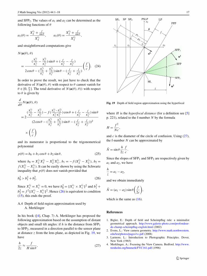
In his book ([4], Chap. 7) A. Merklinger has proposed thefollowing approximation based on the assumption of distantobjects and small tilt angles: if h is the distance from SFP1

to SFP2, measured in a direction parallel to the sensor planeat distance z from the lens plane, as depicted in Fig. 19, wehave

h

2z≈ f

H sin θ, (27)

Fig. 19 Depth of field region approximation using the hyperfocal

where H is the hyperfocal distance (for a definition see [5]p. 221), related to the f-number N by the formula

H = f 2

Nc,

and c is the diameter of the circle of confusion. Using (27),the f-number N can be approximated by

N = sin θh

2z

f

c.

Since the slopes of SFP1 and SFP2 are respectively given bya1 and a2, we have

h

z= a1 − a2,

and we obtain immediately

N = (a1 − a2) sin θ

(f

2c

),

which is the same as (16).

References

1. Bigler, E.: Depth of field and Scheimpflug rule: a minimalistgeometrical approach. http://www.galerie-photo.com/profondeur-de-champ-scheimpflug-english.html (2002)

2. Evens, L.: View camera geometry. http://www.math.northwestern.edu/len/photos/pages/vc.pdf (2008)

3. Larmore, L.: Introduction to Photographic Principles. Dover,New York (1965)

4. Merklinger, A.: Focusing the View Camera. Bedford. http://www.trenholm.org/hmmerk/FVC161.pdf (1996)

http://www.galerie-photo.com/profondeur-de-champ-scheimpflug-english.html

http://www.galerie-photo.com/profondeur-de-champ-scheimpflug-english.html

http://www.math.northwestern.edu/len/photos/pages/vc.pdf

http://www.math.northwestern.edu/len/photos/pages/vc.pdf

http://www.trenholm.org/hmmerk/FVC161.pdf

http://www.trenholm.org/hmmerk/FVC161.pdf


5. Ray, S.F.: Applied Photographic Optics, 3rd edn. Focal Press,Waltham (2002)

6. Scheimpflug, T.: Improved method and apparatus for the system-atic alteration or distortion of plane pictures and images by meansof lenses and mirrors for photography and for other purposes. GBPatent No. 1196, 1904

7. Tillmans, U.: Creative Large Format: Basics and Applications.Sinar AG, Feuerthalen (1997)

8. Wheeler, R.: Notes on view camera geometry. http://www.bobwheeler.com/photo/ViewCam.pdf (2003)

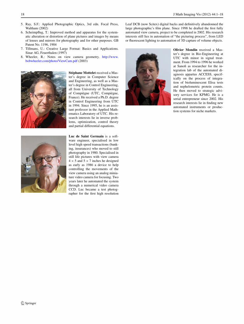
Stéphane Mottelet received a Mas-ter’s degree in Computer Scienceand Engineering, as well as a Mas-ter’s degree in Control Engineering,all from University of Technologyof Compiègne (UTC, Compiègne,France). He received a Ph.D. degreein Control Engineering from UTCin 1994. Since 1995, he is an assis-tant professor in the Applied Math-ematics Laboratory of UTC. His re-search interests lie in inverse prob-lems, optimization, control theoryand partial differential equations.

Luc de Saint Germain is a soft-ware engineer, specialised in lowlevel high speed transactions (bank-ing, insurances) who moved to stillphotography in 1980. Specialised instill life pictures with view camera4 × 5 and 5 × 7 inches he designedas early as 1986 a device to helpcontrolling the movements of theview camera using an analog minia-ture video camera for focusing. Twoyears later he automated the systemthrough a numerical video cameraCCD. Luc became a test photog-rapher for the first high resolution

Leaf DCB (now Scitex) digital backs and definitively abandonned thelarge photographic’s film plane. Since 1998 he drafted the first fullyautomated view camera, project to be completed in 2002. His researchinterests still lies in automation of “the picturing process”, from LEDor fluorescent lighting to automation of 3D capture of volume objects.

Olivier Mondin received a Mas-ter’s degree in Bio-Engineering atUTC with minor in signal treat-ment. From 1994 to 1996 he workedat Sanofi as researcher for the in-tegration lab of the automated di-agnosis appartus ACCESS, specif-ically on the process of integra-tion of bioluminescent Elisa testsand nephelometric protein counts.He then moved to strategic advi-sory services for KPMG. He is aserial entrepreneur since 2002. Hisresearch interests lie in finding newautomated instruments or produc-tion systems for niche markets.

http://www.bobwheeler.com/photo/ViewCam.pdf

http://www.bobwheeler.com/photo/ViewCam.pdf

Smart Depth of Field Optimization Applied to a Robotised View Camera

Documents

Transcript of Smart Depth of Field Optimization Applied to a Robotised View Camera