SMA Facility Location - MIT OpenCourseWare · Optimization ApplicationsOptimization Applications...
48
Facility Location Facility Location Facility Location and Distribution and Distribution and Distribution System Planning System Planning System Planning Thomas L. Magnanti Thomas L. Magnanti
Transcript of SMA Facility Location - MIT OpenCourseWare · Optimization ApplicationsOptimization Applications...

Facility LocationFacility LocationFacility Locationand Distributionand Distributionand Distribution System PlanningSystem PlanningSystem Planning
Thomas L. MagnantiThomas L. Magnanti
Today’s AgendaToday’s Agenda
� Why study facility location? � Issues to be modeled � Basic models
� Fixed charge problems � Core uncapacitated and capacitated
facility location models � Large-scale application (Hunt-
Wesson Foods)
� Why study facility location?� Issues to be modeled� Basic models
� Fixed charge problems� Core uncapacitated and capacitated
facility location models� Large-scale application (Hunt-
Wesson Foods)

Logistics IndustryLogistics Industry� U.S. logistics industry: $900 billion - almost
double the size of the high-tech industry: > 10percent of the U.S. gross domestic product
� 11 per cent of Singapore's GDP with a growth of9 per cent in year 2000
� Singapore Logistics Enhancement &Applications Programme (LEAP) 2001
� Global logistics: $3.43 trillion � 1998, U.S. trucking industry revenues just
under $200 billion � 7.7 million trucks carried over 1 trillion ton
miles of freight
� U.S. logistics industry: $900 billion - almost double the size of the high-tech industry: > 10percent of the U.S. gross domestic product
� 11 per cent of Singapore's GDP with a growth of9 per cent in year 2000
� Singapore Logistics Enhancement &Applications Programme (LEAP) 2001
� Global logistics: $3.43 trillion � 1998, U.S. trucking industry revenues just
under $200 billion� 7.7 million trucks carried over 1 trillion ton
miles of freight

Singapore Retail 21 PlanSingapore Retail 21 Plan

Basic IssueBasic Issue
� Where to locate and how to size facilities?
� How to meet customer demands from the facilities? � Which facility (facilities) serve each
customer? � How much customer demand is met by
each facility?
� Where to locate and how to size facilities?
� How to meet customer demands from the facilities?� Which facility (facilities) serve each
customer?� How much customer demand is met by
each facility?Facilities might be warehouses, retail outlets,
wireless bay stations, communication concentrators

Some Elements of Cost & ServiceSome Elements of Cost & Service
� Transportation Costs � Vehicles, Drivers, Fuel
� Warehousing � Facility Construction/Rental, Handling
Costs, Inventory � Customer Service
� Service Time, Single Sourcing
� Transportation Costs� Vehicles, Drivers, Fuel
� Warehousing � Facility Construction/Rental, Handling
Costs, Inventory� Customer Service
� Service Time, Single Sourcing

Effect of More FacilitiesEffect of More FacilitiesEffect of More Facilities
+++---
Fixed Costs FixedFixed CostsCosts
TransportationCostsTransportationTransportationCostsCosts
System Trade-offsSystem Trade-offs

Effect of “Individualized” Service (e.g., Direct Shipments) Effect of “Individualized”Effect of “Individualized” Service (e.g., Direct Shipments)Service (e.g., Direct Shipments)
+++---
ServiceServiceServiceCostsCostsCosts
System Trade-offsSystem Trade-offs

Nature of CostsNature of Costs
� Fixed Costs � Facility construction/rental � Vehicle purchases & rentals � Personnel (drivers, managers) � Fixed overhead
� Variable Costs � Inventory, handling, fuel
� Fixed Costs� Facility construction/rental� Vehicle purchases & rentals� Personnel (drivers, managers)� Fixed overhead
� Variable Costs� Inventory, handling, fuel

Optimization ApplicationsOptimization Applications
� Hunt-Wesson Foods saves over $1 million per year
� Restructuring North America operations, Proctor and Gamble reduces plants by 20%, saving $200 million/year
� Many, many others (e.g., supplying parts to plants)
� Hunt-Wesson Foods saves over $1 million per year
� Restructuring North America operations, Proctor and Gamble reduces plants by 20%, saving $200 million/year
� Many, many others (e.g., supplying parts to plants)

1919
Facility Location ChallengeFacility Location Challenge

Modeling IssueModeling Issue
� How do we model “lumpiness” of the costs (e.g., fixed costs)?
� How do we model logical conditions (e.g., choice of warehouse locations)?
� How do we model “lumpiness” of the costs (e.g., fixed costs)?
� How do we model logical conditions (e.g., choice of warehouse locations)?

Modeling Fixed CostsModeling Fixed Costs
� Incur fixed cost F if either x > 0 or z > 0 � Suppose x + z < 3/2 (demand limitation) � Incur fixed cost F if either x > 0 or z > 0� Suppose x + z < 3/2 (demand limitation)
Flow x > 0 Flow z > 0
Minimize Fy + other terms subject to y = 1 if either x > 0 or z > 0
Model

Three Models (LP Relaxations)Three Models (LP Relaxations)
Forcing Constraints
Weak Strong
x + z < 3/2 x < 1, z < 1 x + z < 2y x > 0, z > 0 0 < y < 1
Model 1 x + z < 3/2 x < 1, z < 1 x < y, z < y x > 0, z > 0 0 < y < 1
Model 2
x + z < 3y/2 x < 1, z < 1 x < y, z < y x > 0, z > 0 0 < y < 1
Model 3

Geometry (Weak Model)Geometry (Weak Model)
x + z < 2y intersects at y = 3/4
Feasible region with x<1, y<1, z<1, x + z< 3/2
Feasible region with x<1, y<1, z<1, x + z< 3/2
x + z < 3/2 y
x
z
x
y
z
Feasible points

y
x
z
Geometry (Improved Model)Geometry (Improved Model)
x < y, z < y intersects at
x = z = y = 3/4 & at y = 1 w/ x or z =1
x < y, z < yintersects at
x = z = y = 3/4 & at y = 1 w/ x or z =1
x + z < 3/2 y
x
z

y
x
z
Geometry (Strong Model)Geometry (Strong Model)
x + z < 3y/2, x < y, z < y intersects at y = 1
x + z < 3y/2,x < y, z < yintersects at y = 1
Exact representation!Exact representation!
y
x
z

Minimize Fixed + Routing CostsMinimize Fixed + Routing CostsMinimize Fixed + Routing CostsSubject toSubject toSubject to
� Meet customer demand from facilities
� Assign customer only to open facility
�� Meet customerMeet customer demand from facilitiesdemand from facilities
�� Assign customer only toAssign customer only to open facilityopen facility
Core (Uncapacitated) Facility LocationCore (Uncapacitated) Facility Location

Parameters:
Core Facility Location Model
Parameters:
Core Facility Location Model
� Demand di for each customer i � Fixed cost Fj for each facility location j � Cost cij of routing all customer i
demand to facility j = per unit cost times demand di
� Demand di for each customer i� Fixed cost Fj for each facility location j� Cost cij of routing all customer i
demand to facility j = per unit cost times demand di

Decisions: Core Facility Location Model
Decisions: Core Facility Location Model
� Where do we locate facilities? � yj = 1 if we locate facility at location j
� Fraction of service that customer i receives from facility j (xij )
� Where do we locate facilities?� yj = 1 if we locate facility at location j
� Fraction of service that customer i receives from facility j (xij )
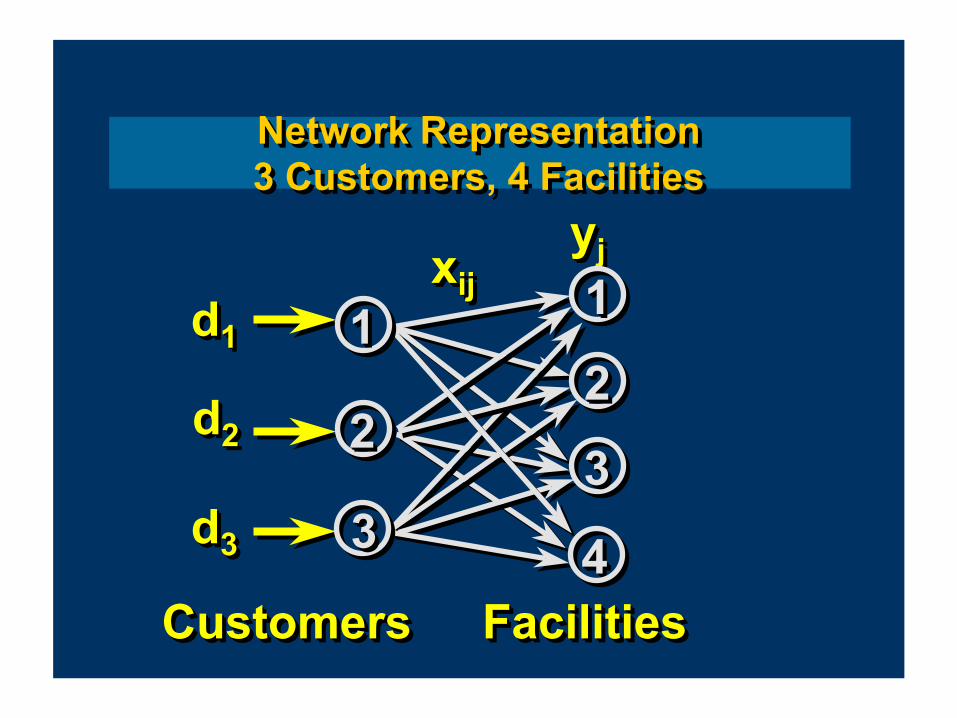
CustomersCustomersCustomers FacilitiesFacilitiesFacilities
xijxxijijyjyyjj
Network Representation 3 Customers, 4 Facilities Network Representation 3 Customers, 4 Facilities
d1dd11
d2dd22
d3dd33
111
222
333 444
111
222
333
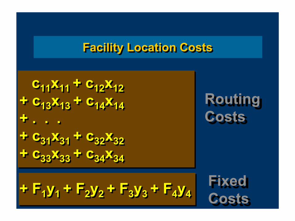
Facility Location CostsFacility Location Costs
c11x11 + c12x12 + c13x13 + c14x14 + . . . + c31x31 + c32x32 + c33x33 + c34x34
+ F1y1 + F2y2 + F3y3 + F4y4
cc1111xx1111 + c+ c1212xx1212 + c+ c1313xx1313 + c+ c1414xx1414 + . . .+ . . .+ c+ c3131xx3131 + c+ c3232xx3232 + c+ c3333xx3333 + c+ c3434xx3434
+ F+ F11yy11 + F+ F22yy22 + F+ F33yy33 + F+ F44yy44
Routing Costs Routing Costs
Fixed Costs Fixed Costs

x11 x12 x13 x14 = 1 x21 x22 x23 x24 = 1 x31 x32 x33 x34 = 1
x11 ≤ y1, x12 ≤ y2, x13 ≤ y3, x14 ≤ y4 x21 ≤ y1, x22 ≤ y2, x23 ≤ y3, x24 ≤ y4 x31 ≤ y1, x32 ≤ y2, x33 ≤ y3, x34 ≤ y4
xx1111 xx1212 xx1313 xx1414 = 1= 1xx2121 xx2222 xx2323 xx2424 = 1= 1xx3131 xx3232 xx3333 xx3434 = 1= 1
xx1111 ≤ yy1,1, xx1212 ≤ yy2,2, xx1313 ≤ yy3,3, xx1414 ≤ yy44xx2121 ≤ yy1,1, xx2222 ≤ yy2,2, xx2323 ≤ yy3,3, xx2424 ≤ yy44xx3131 ≤ yy1,1, xx3232 ≤ yy2,2, xx3333 ≤ yy3,3, xx3434 ≤ yy44
Facilities (Locations)Facilities (Locations)Facilities (Locations)C u s t o m e r s
CCuussttoommeerrss
Constraints: Tabular RepresentationConstraints: Tabular Representation

Σj xij = 1 for all customers i xij ≤ yj for all customers i xij ≥ 0 and facilities j yj = 0 or 1 for all facilities j
ΣΣjj xxijij = 1= 1 for all customers ifor all customers ixxijij ≤ yyjj for all customers ifor all customers ixxijij ≥ 00 and facilities jand facilities jyyjj = 0 or 1= 0 or 1 for all facilities jfor all facilities j
Minimize ΣiΣj cijxij + Σj FjyjMinimizeMinimize ΣΣiiΣΣjj ccijijxxijij ++ ΣΣjj FFjjyyjj
Subject toSubject toSubject to
Model (Uncapacitated Facilities)
Model (Uncapacitated Facilities)
}}

Modeling VariationsModeling Variations
� Open at most three of facilities 1, 6 and 8-11 � y1 + y6 + y8 + y9 + y10 + y11 ≤ 3
� Assign each customer to a single facility � x11 integer, x12 integer, etc.
� Open at most three of facilities 1, 6 and 8-11� y1 + y6 + y8 + y9 + y10 + y11 ≤ 3
� Assign each customer to a single facility� x11 integer, x12 integer, etc.
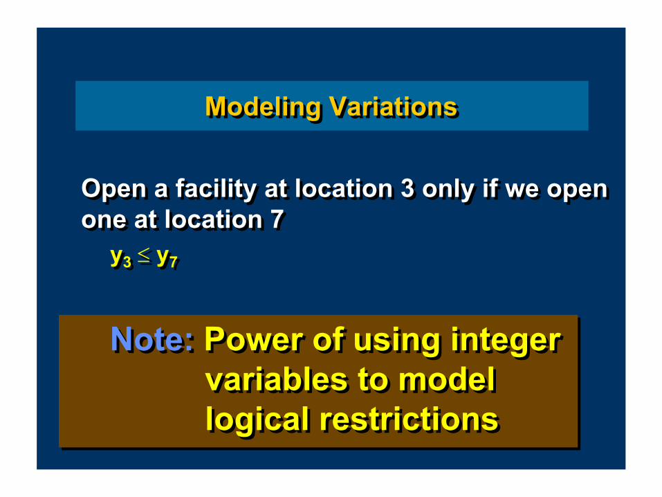
Modeling VariationsModeling Variations
� Open a facility at location 3 only if we open one at location 7 � y3 ≤ y7
� Open a facility at location 3 only if we open one at location 7� y3 ≤ y7
Note: Power of using integer variables to model logical restrictions
Note: Power of using integer variables to model logical restrictions

Modeling EnhancementsModeling Enhancements
� Multiple products � Facility capacities and operating
ranges (min and max throughput ifopen)
� Multi-layered distribution networks � Service restrictions
� Single sourcing � Timing of deliveries
� Inventory positioning and control
� Multiple products� Facility capacities and operating
ranges (min and max throughput ifopen)
� Multi-layered distribution networks� Service restrictions
� Single sourcing� Timing of deliveries
� Inventory positioning and control

Σj xij = 1 for all customers i Σi xij ≤ nyj for all facilities j
xij ≥ 0 for all pairs i,j yj = 0 or 1 for all facilities j
ΣΣjj xxijij = 1= 1 for all customers ifor all customers iΣΣii xxijij ≤ nynyjj for all facilities jfor all facilities j
xxijij ≥ 00 for all pairs i,jfor all pairs i,jyyjj = 0 or 1= 0 or 1 for all facilities jfor all facilities j
Minimize ΣiΣj cijxij + Σj FjyjMinimizeMinimize ΣΣiiΣΣjj ccijijxxijij ++ ΣΣjj FFjjyyjj
Subject toSubject toSubject to
Alternate Model (Uncapacitated Facilities)Alternate Model (Uncapacitated Facilities)
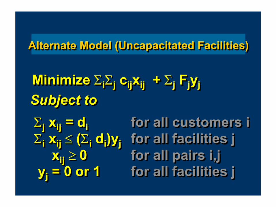
Σj xij = di for all customers i Σi xij ≤ (Σi di)yj for all facilities j
xij ≥ 0 for all pairs i,j yj = 0 or 1 for all facilities j
ΣΣjj xxijij = d= dii for all customers ifor all customers iΣΣii xxijij ≤ ((ΣΣii ddii)y)yjj for all facilities jfor all facilities j
xxijij ≥ 00 for all pairs i,jfor all pairs i,jyyjj = 0 or 1= 0 or 1 for all facilities jfor all facilities j
Minimize ΣiΣj cijxij + Σj FjyjMinimizeMinimize ΣΣiiΣΣjj ccijijxxijij ++ ΣΣjj FFjjyyjj
Subject toSubject toSubject to
Alternate Model (Uncapacitated Facilities)Alternate Model (Uncapacitated Facilities)

Σj xij = di for all customers i xij ≤ diyj for all i, j pairs
Σi xij ≤ CAPj yj for all facilities j xij ≥ 0 for all i, j pairs yj = 0 or 1 for all facilities j
ΣΣjj xxijij = d= dii for all customers ifor all customers ixxijij ≤ ddiiyyjj for all i, j pairsfor all i, j pairs
ΣΣii xxijij ≤ CAPCAPjj yyjj for all facilities jfor all facilities jxxijij ≥ 00 for all i, j pairsfor all i, j pairsyyjj = 0 or 1= 0 or 1 for all facilities jfor all facilities j
Minimize ΣiΣj cijxij + Σj FjyjMinimizeMinimize ΣΣiiΣΣjj ccijijxxijij ++ ΣΣjj FFjjyyjj
Subject toSubject toSubject to
Model (Capacitated Facilities)Model (Capacitated Facilities)
KKjj
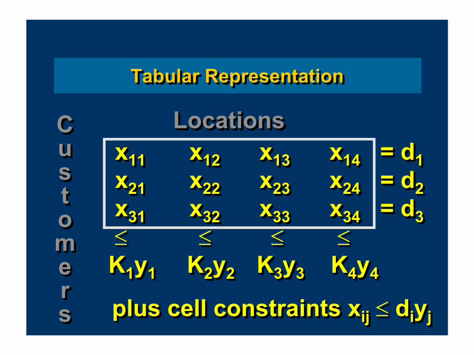
x11 x12 x13 x14 = d1 x21 x22 x23 x24 = d2 x31 x32 x33 x34 = d3 ≤ ≤ ≤ ≤
K1y1 K2y2 K3y3 K4y4
xx1111 xx1212 xx1313 xx1414 = d= d11xx2121 xx2222 xx2323 xx2424 = d= d22xx3131 xx3232 xx3333 xx3434 = d= d33≤ ≤ ≤ ≤KK11yy11 KK22yy22 KK33yy33 KK44yy44
LocationsLocationsLocationsC u s t o m e r s
CCuussttoommeerrss
Tabular RepresentationTabular Representation
plus cell constraints xij ≤ diyjplus cell constraints xxijij ≤ ddiiyyjj

d1dd11
d2dd22
d3dd33
111
222
333 444 444
K1KK11
K2KK22
K3KK33
K4KK44CustomersCustomersCustomers FacilitiesFacilitiesFacilities
xijxxijij yjyyjj
Network RepresentationNetwork Representation
111
222
333
111
222
333

Solution ApproachesSolution Approaches
� Heuristics � Add, drop, and/or exchange � Linear programming relaxation � Bounding (Lagrangian relaxation)
� Optimization methods � Large-scale mixed integer programming � Benders decomposition � Lagrangian relaxation (e.g., dualize capacity
constraints to give uncapacitated facilitylocation subproblem
� Heuristics� Add, drop, and/or exchange� Linear programming relaxation� Bounding (Lagrangian relaxation)
� Optimization methods� Large-scale mixed integer programming� Benders decomposition� Lagrangian relaxation (e.g., dualize capacity
constraints to give uncapacitated facilitylocation subproblem

HuntHunt--Wesson FoodsWesson Foods
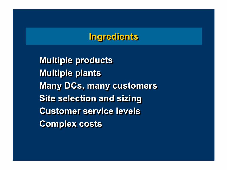
IngredientsIngredients
� Multiple products � Multiple plants � Many DCs, many customers � Site selection and sizing � Customer service levels � Complex costs
� Multiple products� Multiple plants� Many DCs, many customers� Site selection and sizing� Customer service levels� Complex costs

14 plants14 plants14 plants45 DC Choices45 DC Choices45 DC Choices
121 Customer Zones121 Customer Zones121 Customer Zones
FlowsFlowsFlows
17 Product Groups p17 Product Groups17 Product Groups pp
���
���
���
���
���
���
���
���
���
���
iiijjj���
kkk
���
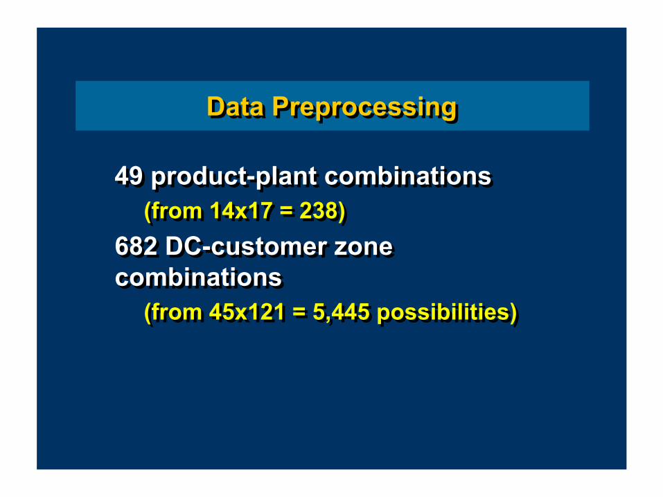
Data PreprocessingData Preprocessing
� 49 product-plant combinations � (from 14x17 = 238)
� 682 DC-customer zone combinations � (from 45x121 = 5,445 possibilities)
� 49 product-plant combinations� (from 14x17 = 238)
� 682 DC-customer zone combinations� (from 45x121 = 5,445 possibilities)
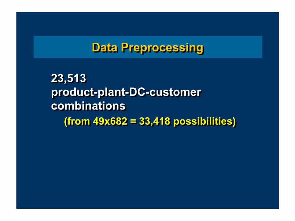
Data PreprocessingData Preprocessing
� 23,513 product-plant-DC-customer combinations � (from 49x682 = 33,418 possibilities)
� 23,513 product-plant-DC-customer combinations� (from 49x682 = 33,418 possibilities)

System RequirementsSystem Requirements
� Data easy to acquire � Inexpensive/quick to run � Easily updated � User-oriented � Flexible (what if capabilities) � Measurable benefits
� Data easy to acquire� Inexpensive/quick to run� Easily updated� User-oriented� Flexible (what if capabilities)� Measurable benefits
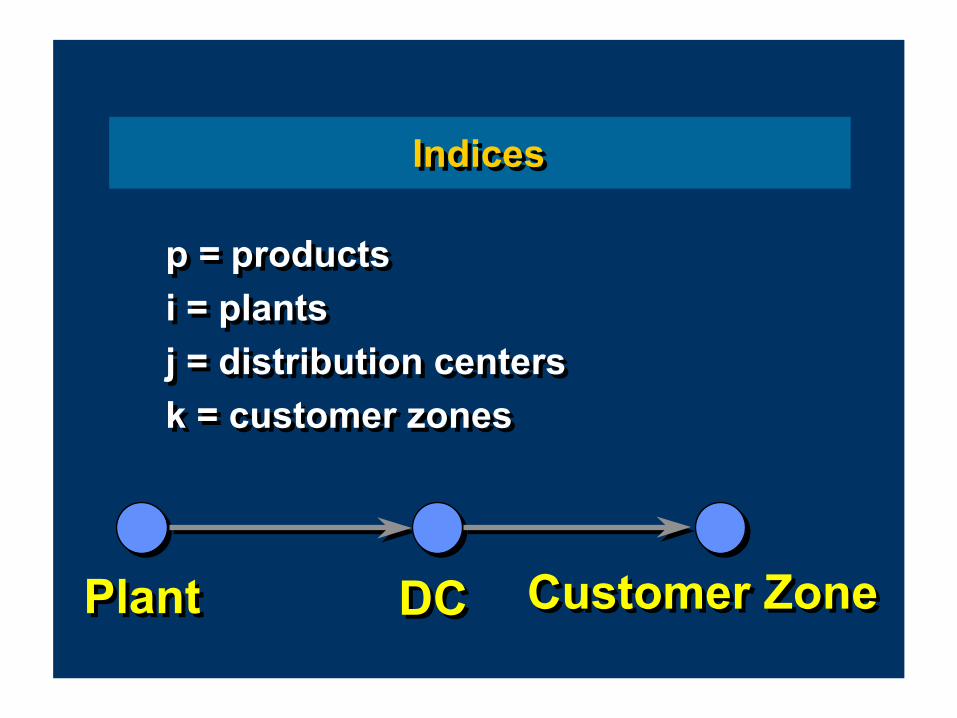
IndicesIndices
� p = products � i = plants � j = distribution centers � k = customer zones
� p = products� i = plants� j = distribution centers� k = customer zones
PlantPlant DCDC Customer ZoneCustomer Zone
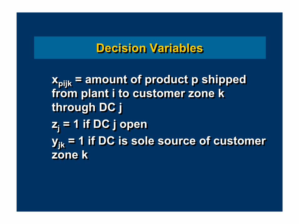
Decision VariablesDecision Variables
� xpijk = amount of product p shipped from plant i to customer zone k through DC j
� zj = 1 if DC j open � yjk = 1 if DC is sole source of customer
zone k
� xpijk = amount of product p shipped from plant i to customer zone k through DC j
� zj = 1 if DC j open� yjk = 1 if DC is sole source of customer
zone k

Σjk xpijk ≤ SpiΣi xpijk = DpkyjkΣj yjk = 1
Vjzj ≤ ΣpkDpkyjk ≤ Vjzj xpijk ≥ 0 zj,yjk = 0 or 1
ΣΣjkjk xxpijkpijk ≤ SSpipiΣΣii xxpijkpijk = D= DpkpkyyjkjkΣΣjj yyjkjk = 1= 1
VVjjzzjj ≤ ΣΣpkpkDDpkpkyyjkjk ≤ VVjjzzjjxxpijkpijk ≥ 00zzjj,y,yjkjk = 0 or 1= 0 or 1
+ Configuration Constraints on y,z+ Configuration Constraints on y,z+ Configuration Constraints on y,z
ConstraintsConstraintsConstraints

Σpijk cpijkxpijk
+ Σj fjzj
+ Σj vjΣpk Dpkyjk
ΣΣpijkpijk ccpijkpijkxxpijkpijk
++ ΣΣjj ffjjzzjj
++ ΣΣjj vvjjΣΣpkpk DDpkpkyyjkjk
Transportation CostTransportation CostTransportation Cost
Fixed DC CostFixed DC CostFixed DC Cost
Variable DC CostVariable DC CostVariable DC Cost
ObjectiveObjective

Model DevelopmentModel Development
� Aggregation of Data � Preselection of Certain Decisions in
Large Applications
� Aggregation of Data� Preselection of Certain Decisions in
Large Applications
Why integer instead of linear programming?
Choice of ModelsChoice of Models

Power of Integer ProgrammingPower of Integer Programming
� Fixed costs � Bounding # of facilities � Precedence constraints � Mandatory service constraints
� Sole sourcing � Service timing
� Fixed costs� Bounding # of facilities� Precedence constraints� Mandatory service constraints
� Sole sourcing� Service timing
Stages in Model DevelopmentStages in Model Development
� Probationary analysis � Analyzing results
� Sensitivity analysis � What if analysis � Priority analysis
� Probationary analysis� Analyzing results
� Sensitivity analysis� What if analysis� Priority analysis

Today’s LessonsToday’s Lessons
� Facility location and distributionimportant in practice
� Geometry of fixed cost modeling � Model choice is important in problem
solving � Strong vs. weak forcing constraints
� Optimization models are able tosolve large-scale practical problems
� Facility location and distributionimportant in practice
� Geometry of fixed cost modeling� Model choice is important in problem
solving� Strong vs. weak forcing constraints
� Optimization models are able tosolve large-scale practical problems

![OEM CATALOG - Crimson Trace catalog. 6 kimber kimber carry ii [red laser sights] ... smith & wesson smith & wesson smith & wesson j-frame. manufacturer model: 163073 • lasergrips](https://static.fdocuments.in/doc/165x107/5b0b3a0d7f8b9aba628d8139/oem-catalog-crimson-trace-catalog-6-kimber-kimber-carry-ii-red-laser-sights.jpg)