Slotting Allowances and Endogenous Shelf Space�

Leslie M. Marxy

Duke UniversityGreg Sha¤erz

University of Rochester

June 2009

Abstract

Slotting allowances are upfront payments that manufacturers make to retailers to obtain

shelf space. They are widespread in the grocery industry and are of concern to antitrust policy

makers because of their potentially adverse e¤ect on retail prices. A popular view is that these

payments arise because retailers have more products from which to choose than they can prof-

itably carry given the availability of shelf space. According to this view, slotting allowances are

caused by the scarcity of shelf space. In this paper, we show that the causality can also go the

other way: the scarcity of shelf space may in part be due to the emergence of slotting allowances.

This has policy implications. Because fewer products can be carried when shelf space is scarce, it

follows that slotting allowances can be anticompetitive even if they have no e¤ect on retail prices.

JEL Classi�cation Codes: D43, L13, L14, L42

�We thank Yaron Yehezkel, two anonymous referees, and seminar participants at Duke, Texas A&M, WashingtonUniversity in St. Louis, and the 4th Annual International Industrial Organization Conference for helpful comments.

yFuqua School of Business, Duke University, Durham, NC 27708; email: marx@duke.edu.zSimon School of Business, University of Rochester, Rochester, NY 14627; email: sha¤er@simon.rochester.edu.

1 Introduction

The typical supermarket carries less than 30,000 products, and yet, at any given time, there

may be over 100,000 products from which to choose.1 To help supermarket retailers decide which

products to carry, it has become common in recent years for them to put at least some of their shelf

space up for bid and let manufacturers compete for their patronage. Those who o¤er the best deals

obtain shelf space. Those who do not risk being excluded altogether. Typically, the manufacturers�

deals include potentially large, upfront payments that are independent of the retailers�subsequent

quantity purchases. These upfront payments are referred to in the trade press as slotting allowances.

Slotting allowances have received a lot of attention from policy makers,2 and there is a growing

academic literature that seeks to identify their competitive e¤ects. One concern is that large,

dominant �rms will buy up scarce shelf space in order to exclude their smaller rivals from the

market.3 According to this view, large �rms may obtain shelf space not necessarily because they

make better products, but because they are willing to pay more to protect their monopoly rents

than small �rms are willing to pay to be competitive (Sha¤er, 2005).4 An alternative view is that

slotting allowances equate supply and demand and thus represent the market price of a scarce asset

(shelf space) which, according to price theory, has optimal allocative properties (Sullivan, 1997).

Under this view, the �rms that o¤er the best deals are the ones whose products generate the largest

private and social bene�t, and thus only the most desirable products will be allocated shelf space.

Both viewpoints take as given the scarcity of shelf space and implicitly assume that slotting

allowances arise in response to this scarcity. By contrast, in this paper, we show that the scarcity

of shelf space itself may depend on the feasibility of slotting allowances in the sense that the

retailer is more likely to limit its shelf space in an environment with slotting allowances than

without. Although this departs from conventional thinking on slotting allowances, the idea we

wish to explore is straightforward and comes from the theory of rent-shifting.5 The choice of how

1According to the Food Marketing Institute, the typical supermarket carries approximately 15,000 products. Atypical superstore (de�ned as a larger supermarket with at least 40,000 square feet of total selling area) carriesapproximately 25,000 products. See http://www:fmi:org=facts� figs=?fuseaction = superfact (18 June, 2009).

2See �Slotting: Fair for Small Business and Consumers? Hearing Before the Senate Committee on Small Business,�106th Congress, 1st Session 386 (1999), and the Federal Trade Commission reports, �Report on the Federal TradeCommission�s Workshop on Slotting Allowances and Other Marketing Practices in the Grocery Industry,� (2001),and �Slotting Allowances in the Retail Grocery Industry: Selected Case Studies in Five Product Categories,�(2003).

3See �The Abuse of Dominance Provisions as Applied to the Retail Grocery Industry,� available at http://cb-bc.gc.ca/epic/internet/incb-bc.nsf/vwGeneratedInterE/ct02317e.html#5.2. See also FTC (2001) and FTC (2003).

4A related concern is that large �rms may have easier access to capital markets and/or be able to obtain better�nancial terms, giving them a tangible advantage over their smaller rivals when funding upfront payments.

5The use of contracts to shift rents among vertically-related �rms was �rst studied by Aghion and Bolton (1987).

1

much shelf space to build can be viewed as a strategic decision by the retailer. By limiting its

shelf space, a retailer can often force manufacturers to compete more vigorously for its patronage,

which then allows it to obtain better terms of trade.6 Slotting allowances can help in this regard by

making the transfer of surplus more e¢ cient. In contrast, when slotting allowances are infeasible,

the main drawback of carrying fewer products� a smaller overall joint pro�t� then becomes more

salient.

Our model has implications for antitrust policy. Typically the concern of antitrust authorities

is whether a dominant �rm can plausibly induce a smaller rival to exit by buying up scarce shelf

space. Reasoning that the dominant �rm will not buy up extra shelf space unless it can be assured

that its rival�s product is the one being excluded and not some unrelated product, the focus has

been on the ancillary provisions that sometimes accompany contracts with slotting allowances. For

example, a contract in which a �rm promises to pay a retailer a lump-sum amount with no mention

of its rivals�products is looked upon more favorably than a contract in which a �rm o¤ers a retailer

a lump-sum payment in exchange for contingencies on the retailer�s sales of rival products.7 In our

model, a prohibition of ancillary provisions in contracts that mention rivals would be ine¤ective,

and it would not address the fundamental problem. This is because the source of the problem is

the scarcity of the shelf space itself and not how the shelf space is allocated among the various

products. By limiting its shelf space, the retailer links all products, whether or not they are

otherwise independent in demand. Thus, irrespective of whether there are ancillary provisions in

a particular manufacturer�s contract that identify which �rms are or are not competitors, some

products will necessarily be excluded.

Slotting allowances do not a¤ect consumer prices in our model, nor do they lead retailers to

make ine¢ cient choices of which products to carry.8 Prices are not a¤ected because manufacturers

obtain their shelf space at the expense of unrelated products, leaving market conditions unchanged,

and product choices are not distorted because, conditional on the available shelf space, the retailer

6The result that the retailer might be able to increase its pro�t by committing to purchase from fewer supplierscan be found in O�Brien and Sha¤er (1997). See also the papers by Dana (2004) and Inderst and Sha¤er (2007).The mechanism at work here, however, is fundamentally di¤erent. In these other models, the contracting takes placesimultaneously. In our model, the contracting occurs sequentially, which allows for the possibility of rent shifting.

7To give an example, consider a contract in which a �rm o¤ers to pay the retailer some amount of money upfront ifthe retailer agrees to purchase at least 80% of its requirements from the �rm. Such a contract features both a slottingallowance and a market-share discount. In its 2001 report on slotting allowances, the Federal Trade Commissionexpressed concern that such contracts might lead to ine¢ cient exclusion and ultimately higher prices for consumers.

8This contrasts with the view that slotting allowances may lower consumer prices because they are an e¢ cientmechanism for the retailer to equate the supply and demand of shelf space (cf. Sullivan, 1997), and the view thatslotting allowances may raise consumer prices because in their absence retailers would use their bargaining powers tonegotiate lower wholesale prices, which would then be passed through to the bene�t of consumers (cf. Sha¤er, 1991).

2

will carry the same products whether or not slotting allowances are feasible. Slotting allowances

are nevertheless anticompetitive in our model because they may contribute to a shortage of retail

shelf space, leading to a reduction in the number and variety of products sold to consumers.

Our model may also shed light on why some retailers seemingly ask for slotting allowances on all

products, while other retailers ask for slotting allowances on some products but not on others, and

only for some product categories, while still other retailers, such as Wal-Mart, allegedly do not ask

for any slotting allowances.9 Previous literature has posited that these observed regularities may

be attributed to the presence or absence of retail competition (Kuksov and Pazgal, 2007), which

may vary from retailer to retailer and by product category, and the presence or absence of non-

contractible manufacturer sales e¤orts (Foros et al., 2008), which may vary by product category.

In Kuksov and Pazgal (2007), for example, slotting allowances arise if and only if downstream

competition is su¢ ciently strong. In contrast, we posit that slotting allowances may be related to

the scarcity of shelf space, and indeed may be contributing to the scarcity of shelf space by serving

as a rent-extraction device. As such, we �nd that there is an inverse relationship between the

observance of slotting allowances and a retailer�s bargaining power. Conditional on having at least

some market power, the more bargaining power a retailer has over its suppliers, the less likely it will

feel a need to limit its shelf space as a means of extracting rent. Slotting allowances do not arise in

our model, for example, when the manufacturers have little bargaining power (or conversely, when

the retailer has most of the bargaining power). Thus, in contrast to Kuksov and Pazgal, who posit

that Wal-Mart does not ask for slotting allowances because it faces less competition in the product

market than do other more traditional retailers. Our model suggests that Wal-Mart does not ask

for slotting allowances simply because it has more bargaining power than these other retailers have.

Our model applies to any product, new or established, that requires shelf space. Other explana-

tions of slotting allowances either tend to be speci�c to new products, or are unrelated to whether

shelf space is scarce.10 For example, in the case of new products, one explanation is that slotting

allowances serve as a screening device to enable a downstream �rm to distinguish high quality

products from low quality products, and another explanation is that slotting allowances allow for

the e¢ cient sharing of the risk of new product failure. The literature in this vein includes Kelly

9See FTC (2003; 58) �One supplier reported that all retailers (except Wal-Mart) charge and are paid slotting...�. This stylized fact has also been reported numerous times in the trade press literature. See, for example, thearticle by Mike Du¤ in DSN Retailing Today, October 13, 2003, �Supermarkets charge them, Wal-Mart doesn�t,�andthe article by Kevin Coupe in Natural Grocery Buyer, Spring 2005, �Mention to them that Wal-Mart doesn�t takeslotting, but simply drives for the lowest possible cost of goods in its desire to o¤er the lowest possible prices.�10There is little empirical literature on the subject, mostly because of the lack of good data, and what there is

focuses on new products (Gundlach and Bloom, 1998; Rao and Mahi, 2003; Israilevich, 2004; Sudhir and Rao, 2006).

3

(1991), Chu (1992), Sullivan (1997), Lariviere and Padmanabhan (1997), Desai (2000), and Bloom,

et al. (2000). Slotting allowances have also been posited to arise for strategic reasons when retailers

have all the bargaining power vis-a-vis their upstream suppliers. Sha¤er (1991) and Foros and Kind

(2008) suggest that retailers will use their bargaining power to obtain slotting allowances rather

than wholesale price concessions in order to avoid dissipating their gains when competing against

other downstream �rms; and in a model with one upstream �rm and competing downstream �rms

that can make take-it-or-leave-it o¤ers, Marx and Sha¤er (2007) show that slotting allowances arise

in equilibrium whenever there is asymmetry downstream (either on the demand or cost side) and

lead to exclusion in the sense that the manufacturer does not obtain distribution at all retail outlets.

The rest of the paper proceeds as follows. We introduce the model and notation in Section 2. In

Section 3, we solve for the equilibrium payo¤s of each �rm for the benchmark case in which slotting

allowances are infeasible. We then show in Section 4 that the retailer may have an incentive to limit

its shelf space in order to obtain better terms of trade, and that slotting allowances weakly increase

these incentives. We discuss the model�s implications and o¤er concluding remarks in Section 5.

2 Model

The simplest model in which to capture the idea that slotting allowances can facilitate rent

extraction, and that this e¤ect is enhanced when shelf space is scarce, is one in which a retailer

must decide which of two products to carry. We assume the two products, X and Y , are produced by

manufacturers X and Y at costs cX(x) and cY (y), respectively, where x is the quantity the retailer

purchases from manufacturer X and y is the quantity the retailer purchases from manufacturer Y .

We also assume that ci(�) is increasing, continuous, and unbounded, with ci(0) = 0 for all i = X;Y .

To capture the idea that shelf-space decisions are often non-localized (i.e., a retailer�s decision

to carry a new product need not imply that it must drop some other product in the same product

category), and to simplify the model�s notation, we assume that X and Y are unrelated and thus

independent in demand. Alternatively, one can think of X and Y as being imperfect substitutes,

with no change in our qualitative results. Thus, the model also extends to settings in which the

retailer�s shelf-space decisions are localized (e.g., which products to put in the freezer section).11

We say that shelf space is scarce if the retailer can only carry one product and plentiful if the

11Although not an issue here, more generally, whether a retailer�s shelf space decisions come at the expense ofcompeting products in the same product category or at the expense of unrelated products in unrelated categories isof great concern to policy makers. Under the former, a manufacturer may be accused of attempting to foreclose itsrivals if it o¤ers slotting allowances, whereas it would not be accused of trying to foreclose its rivals under the latter.

4

retailer can carry both products. Our focus in this paper is on when the retailer would want to

make its shelf space scarce, and how the feasibility of slotting allowances a¤ects this decision.

We model a four stage game. In stage one, the retailer decides whether to make its shelf space

plentiful or scarce. We conceptualize the retailer�s shelf space as consisting of slots of �xed width

and assume, for simplicity, that the retailer can build either one or two slots. We assume that

adequate display and promotion of a product requires exactly one slot of shelf space. Thus, if a

manufacturer obtains a slot, it can satisfy any amount of consumer demand for its product, whereas

if it does not obtain a slot, it is e¤ectively excluded from making any sales. Plentiful shelf space

thus corresponds to building two slots and scarce shelf space corresponds to building one slot. It

follows that the retailer can adequately display and sell both products if and only if shelf space is

plentiful. By contrast, the retailer can display and sell at most one product if shelf space is scarce.

After observing whether the retailer�s shelf space is plentiful or scarce, each manufacturer can

in stage two bid to secure an available slot by o¤ering a slotting allowance.12 We assume these bids

are made simultaneously. The retailer then chooses which o¤er or o¤ers to accept. However, the

retailer can accept only as many o¤ers as there are slots available. If shelf space is scarce, then the

retailer can accept only one manufacturer�s o¤er. In contrast, if shelf space is plentiful, then the

retailer can accept both manufacturers�o¤ers. If an o¤er is accepted, the retailer is paid and the

manufacturer whose slotting allowance was accepted secures the slot. If the retailer rejects both

o¤ers, then no payments are made and control over the slot or slots remains in the retailer�s hands.

Contract negotiations take place in stage three. With one caveat, we assume that these negotia-

tions take place sequentially, with �rst the retailer and manufacturer X negotiating contract TX for

the purchase of manufacturer X�s product and then the retailer and manufacturer Y negotiating

contract TY for the purchase of manufacturer Y �s product.13 The caveat is that if shelf space is

scarce, slotting allowances are feasible, and the only slot has already been secured by manufacturer

i, then there are no contract negotiations between the retailer and manufacturer j in stage three.

We place no restrictions on the form of the contracts other than to assume that each contract

speci�es the retailer�s payment as a function of how much the retailer buys of that manufacturer�s

product only. Thus, we do not allow contracts to depend on both manufacturers� quantities.14

12 In practice, slotting allowances are typically o¤ered in exchange for a �xed amount of shelf space and a pre-speci�ed length of time for which the �rm�s product must be displayed. We simplify here by assuming that slots areindivisible, and that the length of time for which the product must be on display is for the duration of the game.13The assumption that the retailer contracts sequentially with the manufacturers as opposed to simultaneously turns

out to be inconsequential if shelf space is plentiful. However, if shelf space is scarce, then contracting sequentiallyturns out to bene�t manufacturer X and the retailer, who gain from being able to shift rent from manufacturer Y .14Without this restriction, the retailer and manufacturer X could extract all of manufacturer Y �s surplus through

5

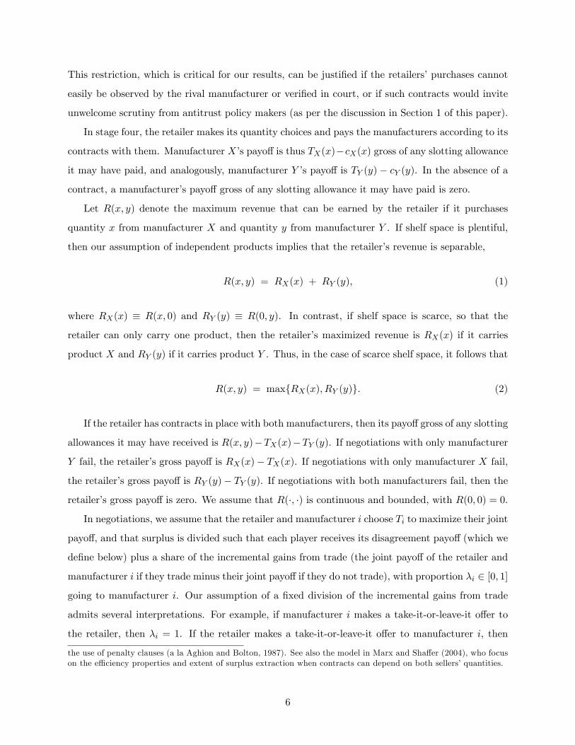
This restriction, which is critical for our results, can be justi�ed if the retailers�purchases cannot

easily be observed by the rival manufacturer or veri�ed in court, or if such contracts would invite

unwelcome scrutiny from antitrust policy makers (as per the discussion in Section 1 of this paper).

In stage four, the retailer makes its quantity choices and pays the manufacturers according to its

contracts with them. Manufacturer X�s payo¤ is thus TX(x)�cX(x) gross of any slotting allowance

it may have paid, and analogously, manufacturer Y �s payo¤ is TY (y)� cY (y). In the absence of a

contract, a manufacturer�s payo¤ gross of any slotting allowance it may have paid is zero.

Let R(x; y) denote the maximum revenue that can be earned by the retailer if it purchases

quantity x from manufacturer X and quantity y from manufacturer Y . If shelf space is plentiful,

then our assumption of independent products implies that the retailer�s revenue is separable,

R(x; y) = RX(x) + RY (y); (1)

where RX(x) � R(x; 0) and RY (y) � R(0; y). In contrast, if shelf space is scarce, so that the

retailer can only carry one product, then the retailer�s maximized revenue is RX(x) if it carries

product X and RY (y) if it carries product Y . Thus, in the case of scarce shelf space, it follows that

R(x; y) = maxfRX(x); RY (y)g: (2)

If the retailer has contracts in place with both manufacturers, then its payo¤gross of any slotting

allowances it may have received is R(x; y)�TX(x)�TY (y). If negotiations with only manufacturer

Y fail, the retailer�s gross payo¤ is RX(x)� TX(x). If negotiations with only manufacturer X fail,

the retailer�s gross payo¤ is RY (y)� TY (y). If negotiations with both manufacturers fail, then the

retailer�s gross payo¤ is zero. We assume that R(�; �) is continuous and bounded, with R(0; 0) = 0.

In negotiations, we assume that the retailer and manufacturer i choose Ti to maximize their joint

payo¤, and that surplus is divided such that each player receives its disagreement payo¤ (which we

de�ne below) plus a share of the incremental gains from trade (the joint payo¤ of the retailer and

manufacturer i if they trade minus their joint payo¤ if they do not trade), with proportion �i 2 [0; 1]

going to manufacturer i. Our assumption of a �xed division of the incremental gains from trade

admits several interpretations. For example, if manufacturer i makes a take-it-or-leave-it o¤er to

the retailer, then �i = 1. If the retailer makes a take-it-or-leave-it o¤er to manufacturer i, then

the use of penalty clauses (a la Aghion and Bolton, 1987). See also the model in Marx and Sha¤er (2004), who focuson the e¢ ciency properties and extent of surplus extraction when contracts can depend on both sellers�quantities.

6

�i = 0. Finally, if the retailer and manufacturer i split the gains from trade equally, then �i = 12 .

We solve for the equilibrium strategies (we restrict attention to pure strategies and contracts for

which optimal quantity choices in stage four exist) of the three players by working backwards. The

equilibrium we identify corresponds to the subgame-perfect equilibrium of the related four-stage

game in which the assumed bargaining solution is embedded in the players�payo¤ functions.

3 Solving the model (the benchmark case)

In order to isolate the e¤ects of slotting allowances on the retailer�s decision of how much shelf

space to build, we must solve the model twice, �rst for the case in which slotting allowances are

infeasible (Section 3), and then for the case in which they are feasible (Section 4). Thus, in this

section, we solve the model for the case in which slotting allowances are infeasible. To calculate the

equilibrium payo¤s of each �rm, let �(x; y) � R(x; y)�cX(x)�cY (y) denote the overall joint payo¤

of the manufacturers and the retailer, and let �XY � maxx;y�0�(x; y) denote its maximized value.

It is also useful to de�ne �X � maxx�0�(x; 0) and �Y � maxy�0�(0; y). Note that if shelf space

is plentiful then �XY = �X +�Y . By contrast, if shelf space is scarce then �XY = maxf�X ;�Y g.

3.1 Stage four � retailer�s quantity choices

Let (x��(TX ; TY ); y��(TX ; TY )) denote the retailer�s pro�t-maximizing quantity choices if it has

contract TX in place with manufacturer X and contract TY in place with manufacturer Y , i.e.,

(x��(TX ; TY ); y��(TX ; TY )) 2 arg max

x;y�0R(x; y)� TX(x)� TY (y): (3)

Note that if shelf space is plentiful, then our assumption that the products are independent implies

that the retailer�s pro�t-maximizing choice of x will depend only on TX , and analogously for the

retailer�s pro�t-maximizing choice of y. In contrast, if shelf space is scarce, then the two products

are necessarily linked in the sense that the retailer can only carry one product, and thus the retailer�s

pro�t-maximizing choices of x and y will in general depend on both manufacturer�s contracts.

If instead negotiations with manufacturer Y have failed, and the retailer only has a contract in

place with manufacturer X; then we denote the retailer�s optimal quantity choice by x�(TX); where

x�(TX) 2 argmaxx�0

RX(x)� TX(x): (4)

7

De�ne y�(TY ) analogously for the case in which negotiations with only manufacturer X have failed.

The quantities x�� and x� (and analogously for y�� and y�) are related given the simple structure

of the model. If shelf space is plentiful, then x�� and x� are the same. Otherwise, if shelf space is

scarce, then x�� = x� if the retailer carries manufacturer X�s product, and x�� 6= x� if otherwise.

3.2 Stage three � negotiations with manufacturers X and Y

We begin by considering the retailer�s negotiation with manufacturer Y , which occurs after its

negotiation with manufacturer X. Taking contract TX as given, contract TY will be chosen to solve

maxTY

R(x��; y��) � TX(x��) � cY (y

��); (5)

such that manufacturer Y earns zero plus its share of the incremental gains from trade

�Y = �Y (R(x��; y��) � TX(x

��)� cY (y��) � (RX(x�)� TX(x�))) ; (6)

where zero is manufacturer Y �s disagreement payo¤ if negotiations with the retailer break down.

Since TX is �xed when TY is chosen, it follows from (5) and (6) that TY will be chosen such that15

(x��(TX ; TY ); y��(TX ; TY )) 2 arg max

x;y�0R(x; y)� TX(x)� cY (y): (7)

If there is no contract between the retailer and manufacturer X, then TY will be chosen to max-

imize �(0; y�) such that manufacturer Y earns �Y�(0; y�) and the retailer earns (1� �Y )�(0; y�).

Thus, manufacturer Y �s payo¤ in this case will be �Y�Y and the retailer�s payo¤will be (1��Y )�Y .

We now consider the retailer�s negotiation with manufacturer X. Because this occurs before

the retailer�s negotiation with manufacturer Y , contract TX will be chosen to solve

maxTX

�(x��; y��)� �Y ; (8)

subject to contract TY �s inducing the retailer to choose (x��; y��) such that

(x��; y��) 2 arg maxx;y�0

R(x; y)� TX(x)� cY (y); (9)

15Given TX , there is no reason to distort the retailer and manufacturer Y �s joint-pro�t-maximizing quantities.

8

and manufacturer X receiving its share of the incremental gains from trade with the retailer

�X = �X (�(x��; y��)� �Y � (1� �Y )�Y ) : (10)

The program in (8) and (10) implies that TX will be chosen to maximize the di¤erence between

�(x��; y��) and manufacturer Y �s pro�t, such that (x��; y��) maximizes the retailer�s joint payo¤

with manufacturer Y , and manufacturer X earns its share of the gains from trade with the retailer.

In solving it, note that x�; x��, and y�� are functions of Tx only, and that (9) implies that

R(x��; y��)� TX(x��)� cY (y��) � maxy�0

R(x�; y)� TX(x�)� cY (y): (11)

In choosing their optimal contract, the retailer and manufacturer X may be able to exploit their

�rst-mover advantage by shifting rents from manufacturer Y . However, their ability to do so is

constrained by the independence of the products, whether shelf space is scarce or plentiful, and by

the inequality in (11). If manufacturer Y �s surplus is fully extracted before (11) binds, then �Y = 0

and TX is chosen such that (x��; y��) 2 argmaxx;y�0�(x; y). However, if the constraint in (11)

binds before manufacturer Y �s surplus is fully extracted, then manufacturer Y �s payo¤ satis�es

�Y = �Y (R(x��; y��)� TX(x��)� cY (y��)� (RX(x�)� TX(x�)))

= �Y

�maxy�0

R(x�; y)� cY (y)�RX(x�)�;

where the �rst line comes from (6), and the second line is obtained under the assumption that the

constraint in (11) binds. In this case, the joint payo¤ of the retailer and manufacturer X is

�(x��; y��)� �Y�maxy�0

R(x�; y)� cY (y)�RX(x�)�;

which is maximized by choosing TX such that

(x��; y��) 2 arg maxx;y�0

�(x; y)

and

x� 2 argminx�0

�Y

�maxy�0

R(x; y)� cY (y)�RX(x)�:

It follows that overall joint payo¤ will be maximized whether or not (11) binds, and that manufac-

9

turer Y �s payo¤ will be zero or �Y minx�0maxy�0 (R(x; y)� cY (y)�RX(x)), whichever is larger.

Proposition 1 For any TX(�) that solves the program in (8)�(10), payo¤s are given by

~�R = �XY � ~�X � ~�Y

~�X = �X (�XY � ~�Y � (1� �Y )�Y )

~�Y = max

�0; �Y min

x�0maxy�0

(R(x; y)� cY (y)�RX(x))�;

where ~�R, ~�X , and ~�Y are the payo¤s of the retailer and manufacturers X and Y , respectively.

Proposition 1 implies that the retailer will carry both products and sell the monopoly quantity

of each product if shelf space is plentiful. And if shelf space is scarce, then the retailer will only

carry the product that o¤ers the higher monopoly pro�t, and it will sell the monopoly quantity

of that product. Thus, if shelf space is scarce and �Y > �X , the retailer will sell the monopoly

quantity of product Y . If �X > �Y , the retailer will sell the monopoly quantity of product X.

3.3 Stages one and two � retailer�s shelf-space decision

Proceeding back to the �rst two stages of the game, we now consider the retailer�s decision of

how much shelf space to build given that slotting allowances are assumed to be infeasible. Clearly,

overall joint payo¤ will be higher if the retailer builds two slots rather than just one slot of shelf

space. (with two slots of shelf space, the maximized overall joint payo¤ is �X +�Y , whereas with

one slot of shelf space, the maximized overall joint payo¤ is maxf�X ;�Y g). But, as we will show,

the retailer would then lose the ability to use its contract with manufacturer X to shift rent from

manufacturer Y . Thus, the retailer faces a tradeo¤; it can earn a larger share of a smaller overall

payo¤, or it can earn a smaller share of a larger overall payo¤. Using Proposition 1, this tradeo¤

can be seen by substituting ~�X into ~�R, simplifying, and then rewriting the retailer�s payo¤ as

~�R = (1� �X)�XY + �X(1� �Y )�Y � (1� �X)~�Y : (12)

This is increasing in the overall joint payo¤, �XY , but decreasing in manufacturer Y �s payo¤, ~�Y .

10

The case of plentiful shelf space

Consider �rst the case in which the retailer builds two slots. In this case, the retailer�s maximized

revenue is R(x; y) = RX(x) +RY (y), and thus, from Proposition 1, manufacturer Y �s payo¤ is

~�Y = maxf0; �Y minx�0

maxy�0

(RY (y)� cY (y))g = �Y�Y :

Substituting this into the retailer�s payo¤ in (12) and simplifying yields

~�R = (1� �X)�X + (1� �Y )�Y : (13)

Notice that when shelf space is plentiful, contract TX has no e¤ect on the negotiations between

the retailer and manufacturer Y (nor would contract TY a¤ect negotiations between the retailer

and manufacturer X if manufacturer Y negotiated �rst). This follows because, as noted previously,

x�� = x� when shelf space is plentiful (and the products are independent), and similarly y�� = y�.

The case of scarce shelf space

Now suppose the retailer builds only one slot. In this case, the retailer�s maximized revenue is

R(x; y) = maxfRX(x); RY (y)g, and thus, from Proposition 1, manufacturer Y �s payo¤ is

~�Y = max

�0; �Y min

x�0maxy�0

(maxfRX(x); RY (y)g � cY (y)�RX(x))�

= maxf0; �Y (�Y �maxx�0

RX(x))g:

Notice that manufacturer Y �s payo¤ is strictly less in this case then when shelf space is plentiful.

The reason is that manufacturer X and the retailer can engage in rent shifting when shelf space is

scarce, something they could not do when shelf space was plentiful. Manufacturer X o¤ers generous

terms that allow the retailer to earn maxx�0RX(x) if it carries manufacturer X�s product instead

of Y �s product, and this limits the retailer�s gains from trade with manufacturer Y . Indeed, when

shelf space is scarce, manufacturer Y earns positive payo¤ if and only if �Y > maxx�0RX(x).

If manufacturer Y �s payo¤ is zero, which is the case if the monopoly value of manufacturer X�s

product is higher, or if maxx�0RX(x) > �Y > �X , then the retailer�s payo¤ in (12) simpli�es to

~�R = (1� �X)�XY + �X(1� �Y )�Y : (14)

11

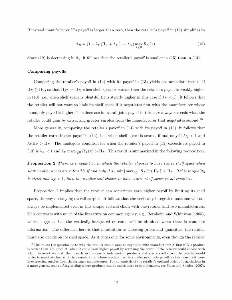
If instead manufacturer Y �s payo¤ is larger than zero, then the retailer�s payo¤ in (12) simpli�es to

~�R = (1� �Y )�Y + �Y (1� �X)maxx�0

RX(x): (15)

Since (12) is decreasing in ~�y, it follows that the retailer�s payo¤ is smaller in (15) than in (14).

Comparing payo¤s

Comparing the retailer�s payo¤ in (14) with its payo¤ in (13) yields an immediate result. If

�X � �Y , so that �XY = �X when shelf space is scarce, then the retailer�s payo¤ is weakly higher

in (13), i.e., when shelf space is plentiful (it is strictly higher in this case if �X < 1). It follows that

the retailer will not want to limit its shelf space if it negotiates �rst with the manufacturer whose

monopoly payo¤ is higher. The decrease in overall joint payo¤ in this case always exceeds what the

retailer could gain by extracting greater surplus from the manufacturer that negotiates second.16

More generally, comparing the retailer�s payo¤ in (14) with its payo¤ in (13), it follows that

the retailer earns higher payo¤ in (14), i.e., when shelf space is scarce, if and only if �X < 1 and

�Y�Y > �X . The analogous condition for when the retailer�s payo¤ in (15) exceeds its payo¤ in

(13) is �X < 1 and �Y maxx�0RX(x) > �X . This result is summarized in the following proposition.

Proposition 2 There exist equilibria in which the retailer chooses to have scarce shelf space when

slotting allowances are infeasible if and only if �Y minfmaxx�0RX(x);�Y g � �X : If this inequality

is strict and �X < 1, then the retailer will choose to have scarce shelf space in all equilibria.

Proposition 2 implies that the retailer can sometimes earn higher payo¤ by limiting its shelf

space, thereby destroying overall surplus. It follows that the vertically-integrated outcome will not

always be implemented even in this simple vertical chain with one retailer and two manufacturers.

This contrasts with much of the literature on common agency, e.g., Bernheim and Whinston (1985),

which suggests that the vertically-integrated outcome will be obtained when there is complete

information. The di¤erence here is that in addition to choosing prices and quantities, the retailer

must also decide on its shelf space. As it turns out, for some environments, even though the retailer

16This raises the question as to why the retailer would want to negotiate with manufacturer X �rst if X�s productis better than Y �s product, when it could earn higher payo¤ by reversing the order. If the retailer could choose withwhom to negotiate �rst, then clearly in the case of independent products and scarce shelf space, the retailer wouldprefer to negotiate �rst with the manufacturer whose product has the smaller monopoly payo¤, as this bene�ts it morein extracting surplus from the stronger manufacturer. For an analysis of the retailer�s optimal order of negotiations ina more general rent-shifting setting where products can be substitutes or complements, see Marx and Sha¤er (2007).

12

does not distort its prices under common agency, it may distort the availability of its shelf space

(for a similar result when contracts are negotiated simultaneously, see O�Brien and Sha¤er, 1997).

The tradeo¤ for the retailer is whether to build one slot in order to capture a larger share of

a smaller overall pro�t, or two slots in order to capture a smaller share of a larger overall pro�t.

Since the di¤erence in overall pro�t is �X , it follows that the larger is �X ; (the right-hand side of

the condition in Proposition 2), the less likely the retailer will opt to build only one slot, all else

being equal. Similarly, the retailer will be less likely to build just one slot the smaller is �Y . This is

because for a given �X , the smaller is �Y , the larger is the retailer�s share of the pro�t when shelf

space is plentiful. Although the retailer�s pro�t share is also decreasing in �Y when shelf space

is scarce, the decrease in this case is not as large given the possibilities for rent shifting. Thus, a

smaller value of �Y makes it less likely that the retailer will build only one slot all else being equal.

4 Slotting allowances and scarce shelf space

It is sometimes argued that the alleged scarcity of shelf space found in practice is a disequilibrium

phenomenon that will be self-correcting in the long run. Proposition 2 suggests otherwise. It implies

that a shortage of shelf space can arise in equilibrium as a consequence of pro�t-maximizing behavior

by retailers with market power. It therefore follows that as long as there exist barriers to entry that

protect retailers�long-run pro�ts, the alleged shortage of shelf-space need not be self-correcting.

Given that a shortage exists, temporary or not, slotting allowances have mostly been viewed

as an e¢ cient mechanism for allocating the scarce shelf space to those products that generate the

highest social surplus. However, this view implicitly takes the scarcity of shelf space as exogenous,

and moreover, as we have seen, the role of slotting allowances in helping ensure that the most

desirable products are carried may be minimal (in our model, the retailer always selects the product

with the higher stand-alone monopoly pro�t regardless of whether slotting allowances are feasible).

4.1 The role of slotting allowances in the retailer�s shelf-space decision

The question we now ask is what impact will slotting allowances have on the scarcity of shelf

space. To consider this, we assume slotting allowances are now feasible and can be o¤ered following

the retailer�s decision whether to make shelf space plentiful or scarce, but before the contract-

negotiation stage. This timing re�ects the status of these payments as a long run variable (e.g.,

an annual payment) that is typically adjusted with less frequency in practice than other contract

13

terms. Many manufacturers claim, for example, that little negotiation takes place over the amount

of the slotting allowance, and that this amount is �known by vendors in advance of discussions.�17

Slotting allowances get them in the door, and then negotiations over the other contract terms begin.

We model slotting allowances as follows. After observing whether shelf space is plentiful or

scarce, each manufacturer has the option of o¤ering a slotting allowance to secure an available slot.

One can think of these o¤ers as being made simultaneously. The retailer then chooses which o¤er

or o¤ers to accept subject to the constraint that it can only accept as many o¤ers as there are slots

available. Acceptance of a manufacturer�s o¤er guarantees a slot for that manufacturer�s product.

We begin the analysis of this revised game by considering �rst the case where shelf space is

plentiful. Two observations make this case trivial to solve. First, by assumption, demand for a

given product does not increase if the manufacturer has two slots versus just one slot, and second,

demand for a given product does not decrease if a slot is given to the other (unrelated) product. It

follows that each manufacturer cares only about securing a single slot for its own product. When

shelf space is plentiful, there is by de�nition a slot available for both products, and thus it follows

that slotting allowances will not arise in equilibrium if shelf space is plentiful (it is a dominant

strategy for both manufacturers to forego o¤ering slotting allowances when shelf space is plentiful).

Now suppose that the retailer�s shelf space is scarce. In this case, the retailer has only one

available slot with which to allocate, and thus one product will necessarily be excluded. As a

result, the manufacturers may be forced to compete for the retailer�s patronage by o¤ering to pay

for shelf space. Let SX � 0 denote manufacturer X�s o¤er and SY � 0 denote manufacturer Y �s

o¤er. One can think of SX and SY as lump-sum payments that are o¤ered to the retailer in exchange

for shelf space of �xed width (a slot) and duration (the rest of the game). Since the retailer has only

one slot available to allocate when shelf space is scarce, it can accept at most one manufacturer�s

o¤er, where acceptance implies that the retailer�s slot is reserved for that manufacturer�s product.

If no o¤er is accepted, the slot remains under the retailer�s control, no payment is made, and the

rest of the game proceeds as above. In contrast, if the retailer accepts an o¤er, the manufacturer

whose o¤er was accepted pays the retailer and then chooses along with the retailer the remaining

contract terms to maximize their joint payo¤, with each receiving its bargaining share of the

incremental gains from trade. It follows that if the retailer accepts manufacturer X�s o¤er, then

17See FTC (2003; 58), �The suppliers�responses suggest that they perceive much less �exibility in whether and howmuch slotting is required.� The FTC report goes on to say (same paragraph) that �Most suppliers also stated thatthe amount of the required slotting payment is set by each retailer and known by vendors in advance of discussions,albeit without written communications. Suppliers stated that very little negotiation over the amount takes place.�

14

the retailer�s payo¤ is (1��X)�X+SX , manufacturer X�s payo¤ is �X�X�SX , and manufacturer

Y �s payo¤ is zero.18 If the retailer accepts manufacturer Y �s o¤er, then the retailer�s payo¤ is

(1� �Y )�Y + SY , manufacturer Y �s payo¤ is �Y�Y � SY , and manufacturer X�s payo¤ is zero.

Which o¤er will be accepted?

Solving the game with slotting allowances is straightforward. There are two cases to consider.

Consider �rst the case in which �Y > �X . Then, if the retailer were to accept manufacturer X�s

o¤er, the joint payo¤ of the retailer and manufacturer Y would be at most �X (manufacturer

X cannot earn negative pro�t in equilibrium), which is less than what their joint payo¤ would

be if the retailer were to accept manufacturer Y �s o¤er instead. This implies that there is no

equilibrium in which manufacturer X�s o¤er is accepted.19 Similarly, if the retailer were to reject

both o¤ers, then the joint payo¤ of the retailer and manufacturer Y would, from Proposition 1, be

�Y � �X�Y minf�Y ;maxx�0RX(x)g, which is weakly less than what their joint payo¤ would be if

the retailer were to accept manufacturer Y �s o¤er (strictly less if �X ; �Y > 0). This implies that if

�X ; �Y > 0, then there is no equilibrium in which shelf space is scarce and both o¤ers are rejected.

It follows that in any equilibrium with scarce shelf space, the retailer will accept manufacturer

Y �s o¤er and earn at least as much pro�t as it could earn if instead it accepted manufacturer X�s

o¤er or rejected both o¤ers. It must also be the case that manufacturer X cannot pro�tably deviate

in equilibrium and that manufacturer Y will o¤er no more than is necessary to obtain the retailer�s

acceptance. Therefore, in any equilibrium with scarce shelf space, the retailer�s payo¤ is given by

~�R =

8<: maxf�X ; (1� �X)�Y + �X(1� �Y )�Y g; if maxx�0RX(x) � �Ymaxf�X ; (1� �Y )�Y + �Y (1� �X)maxx�0RX(x)g; if maxx�0RX(x) < �Y :

(16)

The interpretation of (16) is straightforward. In any equilibrium with scarce shelf space, the

retailer can earn �X if it accepts manufacturer X�s o¤er, and it can earn either the payo¤ in (14)

or the payo¤ in (15) if it rejects both o¤ers (where its payo¤ depends on whether manufacturer Y

would earn positive surplus� which depends on the relationship between maxx�0RX(x) and �Y ).

It follows that (16) represents the retailer�s opportunity cost of accepting manufacturer Y �s o¤er.

18We are implicitly assuming that if the retailer accepts manufacturer X�s o¤er, then it is obligated to carry andsell product X. Alternatively, one might imagine that manufacturer X could obtain the shelf space slot but thenallow the retailer to carry and sell product Y instead. We can show that our results are robust to this possibility.19Formally, there exists a payment SY such that (1� �Y )�Y + SY > �X and �Y�Y � SY > 0. By o¤ering an SY

that satis�es these inequalities, manufacturer Y can induce the retailer to accept its o¤er and make itself better o¤.

15

Comparing the retailer�s payo¤ in (16) with the payo¤s in (14) and (15), it can be seen that,

conditional on shelf space being scarce, the retailer is always weakly (sometimes strictly) better o¤

when slotting allowances are feasible than when they are not. Intuitively, the retailer cannot be

worse o¤ with slotting allowances because it can always reject both o¤ers and guarantee itself the

minimum of the payo¤s in (14) and (15). And it can sometimes be better o¤ (e.g., when �X ; �Y = 1)

because the auctioning of scarce shelf space forces the weaker manufacturer to compete away its

entire surplus even if this manufacturer would otherwise have been able to earn positive payo¤.

It follows that since the retailer can always choose whether to restrict its shelf space, the

feasibility of slotting allowances cannot make the retailer worse o¤. Comparing the retailer�s payo¤

in (16) with its payo¤ in (13), it also follows that the feasibility of slotting allowances may contribute

to the scarcity of shelf space. Since the retailer earns at least �X when shelf space is scarce and

slotting allowances are permitted, a su¢ cient condition for the retailer to prefer to have one slot is

�X > (1� �X)�X + (1� �Y )�Y ;

which holds if and only if �X�X > (1 � �Y )�Y . Combining this condition with the condition

�Y minfmaxx�0RX(x);�Y g � �X from Proposition 2, yields the �rst half of Proposition 3 below.

Now consider the alternative case in which �X � �Y . Then the analogue to (16) is

~�R = maxf�Y ; (1� �X)�X + �X(1� �Y )�Y g; (17)

from which it follows that the retailer will strictly prefer to build one slot if and only if

�Y > (1� �X)�X + (1� �Y )�Y ;

or in other words if and only if �Y�Y > (1� �X)�X . This yields the second half of Proposition 3.

Proposition 3 Assume slotting allowances are feasible. If �Y > �X ; there exist equilibria in

which the retailer chooses scarce shelf space if and only if �Y minfmaxx�0RX(x);�Y g � �X or

�X�X � (1� �Y )�Y ; and scarce shelf space arises in all equilibria if �X < 1 and either inequality

is strict. If �X > �Y ; the retailer chooses scarce shelf space if and only if �Y�Y � (1 � �X)�X ;

and scarce shelf space arises in all equilibria if the inequality is strict.

Conventional wisdom suggests that slotting allowances arise in response to scarce shelf space. In

16

this view, the scarcity of shelf space is assumed to be exogenous. Here, we have shown that slotting

allowances do not arise when shelf space is plentiful, and in that sense our �ndings support the view

that scarce shelf space causes slotting allowances. However, our �ndings also imply that causality

can go the other way� the scarcity of shelf space may, in part, be caused by slotting allowances.

This suggests that slotting allowances may be contributing to the scarcity of retail shelf space.

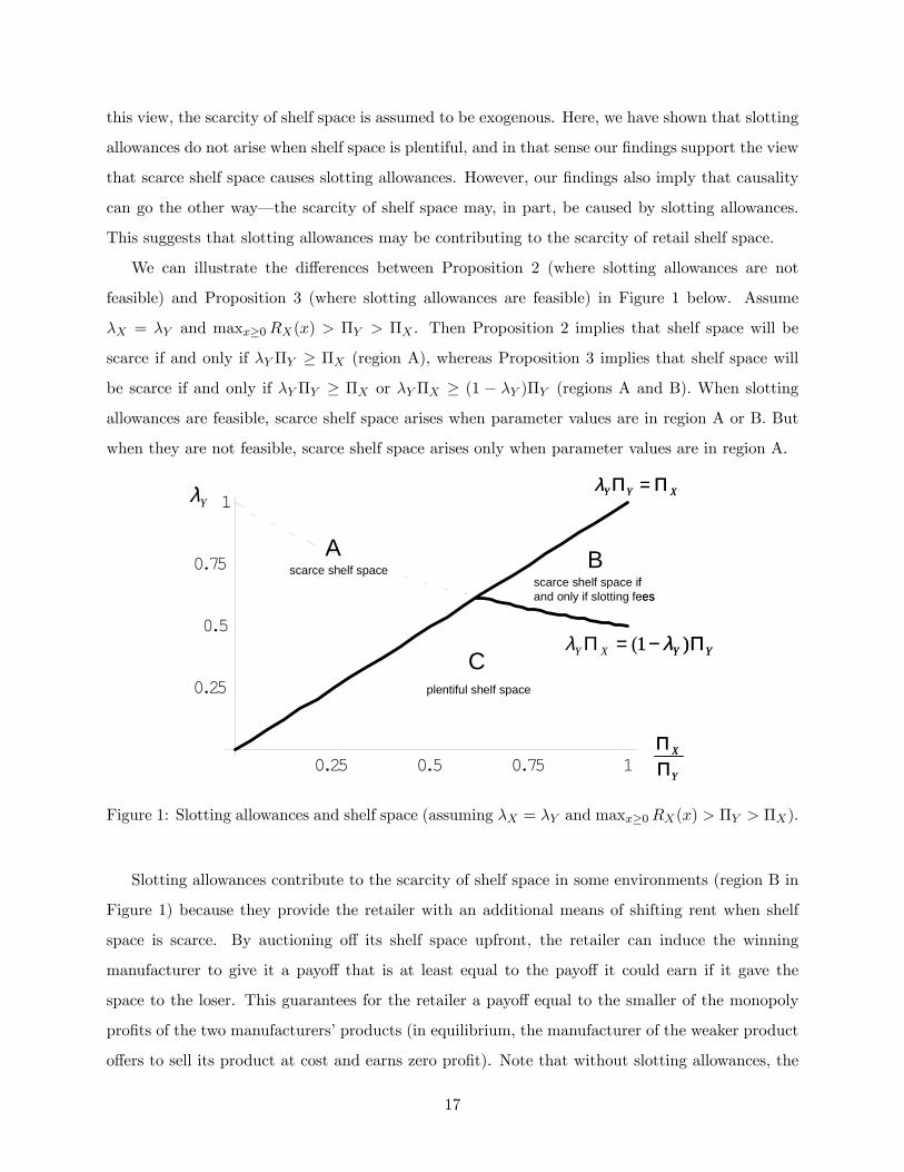
We can illustrate the di¤erences between Proposition 2 (where slotting allowances are not

feasible) and Proposition 3 (where slotting allowances are feasible) in Figure 1 below. Assume

�X = �Y and maxx�0RX(x) > �Y > �X . Then Proposition 2 implies that shelf space will be

scarce if and only if �Y�Y � �X (region A), whereas Proposition 3 implies that shelf space will

be scarce if and only if �Y�Y � �X or �Y�X � (1 � �Y )�Y (regions A and B). When slotting

allowances are feasible, scarce shelf space arises when parameter values are in region A or B. But

when they are not feasible, scarce shelf space arises only when parameter values are in region A.

0.25 0.5 0.75 1

0.25

0.5

0.75

1

Y

X

ΠΠ

Yλ

A

C

scarce shelf space

plentiful shelf space

scarce shelf space ifand only if slotting fees

B

XYY Π=Πλ

YYXY Π−=Π )1( λλ

0.25 0.5 0.75 1

0.25

0.5

0.75

1

Y

X

ΠΠ

Yλ

A

C

scarce shelf space

plentiful shelf space

scarce shelf space ifand only if slotting fees

B

XYY Π=Πλ

YYXY Π−=Π )1( λλ

Figure 1: Slotting allowances and shelf space (assuming �X = �Y and maxx�0RX(x) > �Y > �X):

Slotting allowances contribute to the scarcity of shelf space in some environments (region B in

Figure 1) because they provide the retailer with an additional means of shifting rent when shelf

space is scarce. By auctioning o¤ its shelf space upfront, the retailer can induce the winning

manufacturer to give it a payo¤ that is at least equal to the payo¤ it could earn if it gave the

space to the loser. This guarantees for the retailer a payo¤ equal to the smaller of the monopoly

pro�ts of the two manufacturers�products (in equilibrium, the manufacturer of the weaker product

o¤ers to sell its product at cost and earns zero pro�t). Note that without slotting allowances, the

17

retailer has no such guarantee. Whether shelf space is plentiful or scarce, the retailer�s payo¤ in

the absence of slotting allowances is decreasing in the manufacturers�bargaining powers and is zero

in the polar case in which both manufacturers can make take-it-or-leave-it o¤ers. In contrast, the

retailer always earns positive payo¤ with slotting allowances when shelf space is scarce. Thus, it

follows that slotting allowances may contribute to the scarcity of shelf space and be particularly

valuable to retailers that have local monopoly power but otherwise have little bargaining power.

4.2 Bargaining power and slotting allowances

The retailer�s decision whether to limit its shelf space, and the extent to which the feasibil-

ity of slotting allowances contributes to this decision, depends on the retailer�s bargaining power.

Surprisingly, we see from Proposition 3 that there is an inverse relationship between the retailer�s

bargaining power with respect to each manufacturer and whether slotting allowances arise in equi-

librium.20 Slotting allowances are less likely to arise in equilibrium when the retailer has more

bargaining power (when �X and �Y are low) because with higher bargaining power the focus of the

retailer shifts toward maximizing the overall pro�t rather than limiting its shelf space to extract

rent. Slotting allowances do not arise, for example, if the retailer can make take-it-or-leave-it o¤ers

(�X = �Y = 0). This may explain why a retailer like Wal-Mart, which has high bargaining power

vis-a-vis its suppliers, allegedly does not avail itself of these payments. We call this the �Wal-Mart

phenomenon.� The idea is that the usual tradeo¤ of whether to opt for a larger share of a smaller

overall pro�t or a smaller share of a larger overall pro�t does not apply to Wal-Mart because it can

already capture most or all of the pro�t. Hence, Wal-Mart prefers to have plentiful shelf space.

The Wal-Mart phenomenon is unusual in that Wal-Mart�s bargaining power is thought to be

high whether it is dealing with small manufacturers of produce or potentially large manufacturers

of di¤erentiated, consumer packaged goods. More generally, however, one can imagine that a

retailer may have high bargaining power with respect to suppliers in some product classes, but low

bargaining power with respect to suppliers in other product classes. If the retailer�s shelf space

decisions are localized (for example, products that require freezer space are competing only against20 In our model, the retailer has some market power even if the manufacturers make take-it-or-leave-it o¤ers, as the

manufacturers have no alternative retailer to go to if they want to sell to the local consumers. For this reason, theretailer earns positive pro�t even when the manufacturers have all the bargaining power. Therefore, a more completeinterpretation of our result is the following. First, suppose that the retailer does not have any market power, in thatthere are many potential retailers that each manufacturer can turn to. Clearly, in such a case, the retailer cannotbene�t from limiting its shelf space (the manufacturers will go to another retailer), so slotting allowances will not arisein equilibrium. Second, as we have shown, slotting allowances do not arise if the retailer can make take-it-or-leave-ito¤ers. These polar cases suggest that while the retailer must have market power (few alternative retailers) for slottingallowances to arise, it cannot have signi�cant bargaining power. We thank Yaron Yehezkel for this observation.

18

themselves and not against products that do not need refrigeration), then it is possible that a

given retailer may want strategically to limit its shelf space and obtain slotting allowances for some

product categories, but not limit its shelf space and thus not obtain slotting allowances for other

product categories. In this case, our results imply that the incidence of slotting allowances will be

higher in those product categories in which manufacturers have relatively more bargaining power.

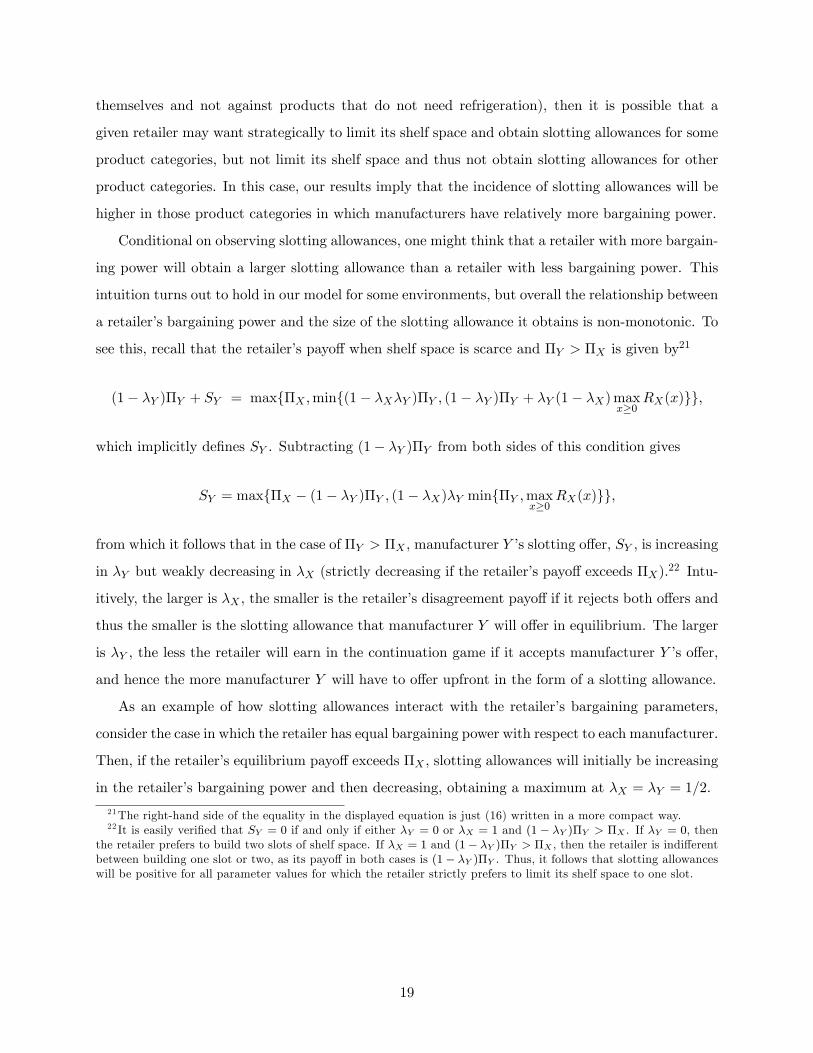
Conditional on observing slotting allowances, one might think that a retailer with more bargain-

ing power will obtain a larger slotting allowance than a retailer with less bargaining power. This

intuition turns out to hold in our model for some environments, but overall the relationship between

a retailer�s bargaining power and the size of the slotting allowance it obtains is non-monotonic. To

see this, recall that the retailer�s payo¤ when shelf space is scarce and �Y > �X is given by21

(1� �Y )�Y + SY = maxf�X ;minf(1� �X�Y )�Y ; (1� �Y )�Y + �Y (1� �X)maxx�0

RX(x)gg;

which implicitly de�nes SY . Subtracting (1� �Y )�Y from both sides of this condition gives

SY = maxf�X � (1� �Y )�Y ; (1� �X)�Y minf�Y ;maxx�0

RX(x)gg;

from which it follows that in the case of �Y > �X , manufacturer Y �s slotting o¤er, SY , is increasing

in �Y but weakly decreasing in �X (strictly decreasing if the retailer�s payo¤ exceeds �X).22 Intu-

itively, the larger is �X , the smaller is the retailer�s disagreement payo¤ if it rejects both o¤ers and

thus the smaller is the slotting allowance that manufacturer Y will o¤er in equilibrium. The larger

is �Y , the less the retailer will earn in the continuation game if it accepts manufacturer Y �s o¤er,

and hence the more manufacturer Y will have to o¤er upfront in the form of a slotting allowance.

As an example of how slotting allowances interact with the retailer�s bargaining parameters,

consider the case in which the retailer has equal bargaining power with respect to each manufacturer.

Then, if the retailer�s equilibrium payo¤ exceeds �X , slotting allowances will initially be increasing

in the retailer�s bargaining power and then decreasing, obtaining a maximum at �X = �Y = 1=2.

21The right-hand side of the equality in the displayed equation is just (16) written in a more compact way.22 It is easily veri�ed that SY = 0 if and only if either �Y = 0 or �X = 1 and (1� �Y )�Y > �X . If �Y = 0, then

the retailer prefers to build two slots of shelf space. If �X = 1 and (1� �Y )�Y > �X , then the retailer is indi¤erentbetween building one slot or two, as its payo¤ in both cases is (1� �Y )�Y . Thus, it follows that slotting allowanceswill be positive for all parameter values for which the retailer strictly prefers to limit its shelf space to one slot.

19

4.3 Slotting allowances, welfare, and pro�ts

Our results have implications for social welfare and the distribution of pro�ts (who gains and

who loses). Notice that if shelf space is plentiful, then the retailer sells both products and the overall

joint payo¤ is �X+�Y . But if shelf space is scarce, then the retailer sells only one product and the

overall joint payo¤ is maxf�X ;�Y g. In both cases, consumers face monopoly prices, which is true

whether or not slotting allowances are feasible. Thus, conditional on the availability of shelf space,

it follows that slotting allowances do not a¤ect product selection or retail prices. However, as we

have seen, the feasibility of slotting allowances a¤ects whether shelf space is scarce. In particular,

it is seen from Propositions 2 and 3 that when slotting allowances are feasible, the retailer is more

likely to limit its shelf space (see region B in Figure 1). When this happens (i.e., when parameter

values are in this region), consumers are worse o¤ with slotting allowances than without. Without

slotting allowances, consumers would be able to select between products X and Y , each priced at

the monopoly price. With slotting allowances, consumers would only be able to select product Y ,

and there would be no change in product Y �s price. Since overall pro�ts are also lower in region B

with slotting allowances than without, it follows that welfare is unambiguously lower in this region.

Turning to the distribution of �rm pro�ts, the retailer is weakly better o¤ with slotting al-

lowances, and when �Y > �X , manufacturer X is weakly worse o¤. Slotting allowances add to the

retailer�s pro�t when the monopoly pro�t of the losing manufacturer�s product exceeds what the

retailer could earn if it rejected both o¤ers or built two slots of shelf space. Given �Y > �X , it

follows that slotting allowances contribute to the retailer�s pro�t if and only if �X is larger than the

retailer�s payo¤ in (14) and (15), which for maxx�0RX(x) � �Y , implies that �X > (1��X�Y )�Y ,

and larger than its payo¤ when shelf space is plentiful, which implies that �X�X > (1� �Y )�Y .

The upper envelope of these two inequalities is shown in Figure 2. For all points in regions A0

and B, the retailer is better o¤ with slotting allowances. For all points in regions A and C, the

retailer is indi¤erent to slotting allowances. Thus, for a given �Y , the retailer is more likely to

gain from slotting allowances the larger is �X relative to �Y (the higher is the guaranteed payo¤

from slotting allowances). And, for a given ratio of �X to �Y , the retailer is more likely to gain

from slotting allowances the larger is �Y (the higher is manufacturer Y �s bargaining power). Since

manufacturer X�s pro�t decreases to zero when slotting allowances are feasible and shelf space is

scarce, manufacturer X is worse o¤ in regions A, A0, and B. However, there is no change in its

pro�t in region C because shelf space is plentiful in this case with or without slotting allowances.

20

0.25 0.5 0.75 1

0.25

0.5

0.75

1

Y

X

ΠΠ

Yλ

A

C

retailer no changeY better offX worse offwelfare no change

no change

retailer better offY worse offX worse offwelfare decrease

B

XYY Π=Πλ

YYXY Π−=Π )1( λλ

A'retailer better offY better offX worse offwelfare no change

YYXX Π−=Π )1( λλ

0.25 0.5 0.75 1

0.25

0.5

0.75

1

Y

X

ΠΠ

Yλ

A

C

retailer no changeY better offX worse offwelfare no change

no change

retailer better offY worse offX worse offwelfare decrease

B

XYY Π=Πλ

YYXY Π−=Π )1( λλ

A'A'retailer better offY better offX worse offwelfare no change

YYXX Π−=Π )1( λλ

Figure 2: Slotting allowances and pro�ts (assuming �X = �Y and maxx�0RX(x) > �Y > �X):

Manufacturer Y gains from slotting allowances in region A since manufacturer X loses, the

retailer�s pro�t is unchanged, and overall joint payo¤ is unchanged. In region A0, the retailer picks

up some of the pro�t lost by manufacturer X, but manufacturer Y still gains because its payo¤ in

this region, �Y � �X , exceeds its payo¤ in the absence of slotting allowances when shelf space is

scarce, maxf0; �Y (�Y �maxx�0RX(x))g. In region B, manufacturer Y earns �Y ��X if slotting

allowances are feasible and �Y�Y otherwise. This implies that manufacturer Y �s payo¤ is higher in

region B with slotting allowances if and only if (1��Y )�Y > �X . But for all points in the interior

of region B, �x�X > (1� �Y )�Y . Hence, manufacturer Y loses in region B. However, there is no

change in manufacturer Y �s payo¤ in region C because shelf space is always plentiful in this case.

5 Conclusion

Slotting allowances have long been of concern in antitrust. They have been the subject of

numerous congressional hearings and the focal point of two recent Federal Trade Commission reports

on marketing practices in the retail grocery industry. Conventional wisdom suggests that the growth

in slotting allowances can be attributed to the imbalance between the number of products (new

and established) that are available for the retailer to choose from at any given time and the number

of products that the retailer can pro�tably carry given its limited shelf space. In contrast, we show

21

that slotting allowances may in fact also be contributing to the scarcity of retail shelf space.

In our model, slotting allowances allow the retailer to capture more e¢ ciently the value of its

shelf space when shelf space is scarce. By itself, this e¤ect is welfare neutral. Slotting allowances in

this case serve only to transfer rents from the weaker manufacturer to the stronger manufacturer

and, for some parameters, from the weaker manufacturer to the retailer. However, the problem

is that this same mechanism may also induce the retailer to limit its shelf space when shelf space

would otherwise be plentiful. This e¤ect tends to reduce welfare and can harm both manufacturers.

Welfare decreases when shelf space is scarce because consumers su¤er from reduced product choice

but do not bene�t from lower prices. The manufacturers are worse o¤ when shelf space would

otherwise be plentiful because overall joint pro�t is lower, but the retailer�s pro�t is higher.

Our results point to a new source of welfare loss. Policy makers have previously been concerned

with whether slotting allowances would lead to higher or lower retail prices, and whether dominant

manufacturers might abuse slotting allowances by buying up scarce shelf space in order to foreclose

smaller rivals with better products. These concerns have caused policy makers in speci�c cases

to consider whether the excluded �rms have equal access to capital markets, whether slotting

allowances are coupled with exclusivity provisions (e.g., whether the dominant �rm requires that

the downstream �rm not sell its competitor�s product), and whether there are scale economies in

production that may prevent an excluded �rm from e¤ectively competing elsewhere in the market.

However, in our model, there is no e¤ect on retail pricing, and the better product is always chosen

conditional on the availability of shelf space. Instead, we �nd that welfare may be lower because

slotting allowances may induce the retailer to limit its shelf space. This suggests that slotting

allowances may be harmful even if they are not accompanied by exclusivity provisions, the market

does not exhibit scale economies in production, and access to capital markets is not a concern.

Our results also have testable implications. In a recent study on slotting allowances, the Federal

Trade Commission (2003, p.vi) concluded that, �For the �ve product categories during the time

periods of this study, the surveyed retailers�data on the frequency of slotting fees varied widely

between and within product categories, across retailers, and across a particular retailer�s regions.�

The Federal Trade Commission (2003, p.vii) further concluded that, �For the seven retailers during

the time periods of this study, slotting allowances were more prevalent for ice cream and salad

dressing products than for bread and hot dog products.� In some instances, the Federal Trade

Commission found that slotting allowances were paid on all new products in a particular category.

In other categories, they found that few if any slotting allowances were paid on the new products.

22

Kuksov and Pazgal (2007) and Foros et al (2008) have previously posited that these �ndings

may be accounted for by di¤erences in the intensity of retail competition, and by the importance of

non-contractible demand-enhancing investments by manufacturers, respectively.23 In contrast, we

suggest that these �ndings may also (or instead) be due to di¤erences in a retailer�s bargaining power

with respect to each manufacturer and with respect to each other. In particular, we have shown that

the incidence of slotting allowances may be inversely related to each retailer�s bargaining power.

If a retailer with market power has all the bargaining power with respect to each manufacturer,

then the retailer extracts all the available surplus in the market and slotting allowances do not

arise. But slotting allowances will arise if the manufacturers have all the bargaining power because

then the retailer will want to limit its shelf space all else being equal in order to earn some pro�t.

For intermediate levels of bargaining power, the retailer is more likely to limit its shelf space (and

therefore slotting allowances are more likely to arise) the less bargaining power it has. This accords

well with the observation that slotting allowances tend to arise for items such as ice cream and salad

dressing, where strong brand names exist, but not for items where strong brand names do not exist,

such as bread and hot dogs. This also accords well with the observation that Wal-Mart, a retailer

that is thought to have a lot of bargaining power, allegedly does not accept slotting allowances.

We have also shown that, conditional on receiving slotting allowances, there is a non-monotonic

relationship between a retailer�s bargaining power and the magnitude of any slotting allowances it

receives. Retailers with low bargaining power vis-a-vis their suppliers will tend to negotiate roughly

the same level of slotting allowances as retailers with high bargaining power, whereas retailers with

moderate bargaining power will be able to negotiate the highest slotting allowances. In principle,

these �ndings can be tested, but, to our knowledge, the data needed to do so is not yet available.

23An alternative explanation for why slotting allowances may be observed for branded goods but less so for un-branded goods is that suppliers of unbranded goods may face binding credit constraints. This accords with a concernof policy makers that slotting allowances may place small manufacturers at a disadvantage for reasons other than themerits of their products (see the discussion above in Section 1). We thank an anonymous referee for this insight.

23

A Appendix

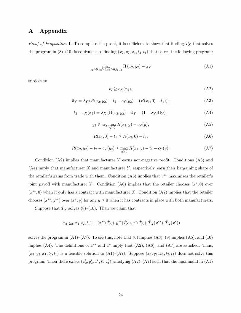
Proof of Proposition 1. To complete the proof, it is su¢ cient to show that �nding TX that solves

the program in (8)�(10) is equivalent to �nding (x2; y2; x1; t2; t1) that solves the following program:

maxx2�0;y2�0;x1�0;t2;t1

�(x2; y2)� ~�Y (A1)

subject to

t2 � cX(x2); (A2)

~�Y = �Y (R(x2; y2)� t2 � cY (y2)� (R(x1; 0)� t1)) ; (A3)

t2 � cX(x2) = �X (�(x2; y2)� ~�Y � (1� �Y )�Y ) ; (A4)

y2 2 argmaxy�0

R(x2; y)� cY (y); (A5)

R(x1; 0)� t1 � R(x2; 0)� t2; (A6)

R(x2; y2)� t2 � cY (y2) � maxy�0

R(x1; y)� t1 � cY (y): (A7)

Condition (A2) implies that manufacturer Y earns non-negative pro�t. Conditions (A3) and

(A4) imply that manufacturer X and manufacturer Y , respectively, earn their bargaining share of

the retailer�s gains from trade with them. Condition (A5) implies that y�� maximizes the retailer�s

joint payo¤ with manufacturer Y . Condition (A6) implies that the retailer chooses (x�; 0) over

(x��; 0) when it only has a contract with manufacturer X. Condition (A7) implies that the retailer

chooses (x��; y��) over (x�; y) for any y � 0 when it has contracts in place with both manufacturers.

Suppose that T̂X solves (8)�(10). Then we claim that

(x2; y2; x1; t2; t1) � (x��(T̂X); y��(T̂X); x�(T̂X); T̂X(x��); T̂X(x�))

solves the program in (A1)�(A7). To see this, note that (6) implies (A3), (9) implies (A5), and (10)

implies (A4). The de�nitions of x�� and x� imply that (A2), (A6), and (A7) are satis�ed. Thus,

(x2; y2; x1; t2; t1) is a feasible solution to (A1)�(A7). Suppose (x2; y2; x1; t2; t1) does not solve this

program. Then there exists (x02; y02; x

01; t

02; t

01) satisfying (A2)�(A7) such that the maximand in (A1)

24

is greater at (x02; y02; x

01; t

02; t

01) than at (x2; y2; x1; t2; t1): Consider contract T

0X de�ned by:

T 0X(x) �

8>>><>>>:t02; if x = x02

t01; if x = x01

1; otherwise.

Because (x02; y02; x

01; t

02; t

01) satis�es (A2)�(A7) it follows that (x

��(T 0X); y��(T 0X)) = (x02; y

02) and

x�(T 0X) = x01; and so T

0X satis�es (9)�(10). Thus, T

0X is a feasible solution to (8)�(10) and gives the

retailer and manufacturer X higher joint payo¤ than T̂X ; a contradiction. Thus, (x2; y2; x1; t2; t1) �

(x��(T̂X); y��(T̂X); x

�(T̂X); T̂X(x��); T̂X(x

�)) solves (A1)�(A7).

Now suppose T̂X is not an equilibrium contract. Then T̂X does not solve (8)�(10). Because T̂X

is not an equilibrium contract, the contract T 00X ; where

T 00X(x) �

8>>><>>>:T̂X(x

��(T̂X)); if x = x��(T̂X)

T̂X(x�(T̂X)); if x = x�(T̂X)

1; otherwise,

is also not an equilibrium contract. If T 00X is not a feasible solution to (8)�(10), then at least one of

(9)�(10) is violated. Consider (x2; y2; x1; t2; t1) � (x��(T̂X); y��(T̂X); x

�(T̂X); T̂X(x��); T̂X(x

�)): If

T 00X violates (9), then (x2; y2; x1; t2; t1) violates at least one of (A2)�(A7). If T00X violates (10), then

(x2; y2; x1; t2; t1) violates (A4). If T 00X is a feasible solution to (8)�(10), then there exists T 000X also

feasible but giving a higher value of the maximand in (8). Then (x2; y2; x1; t2; t1) and

(x0002 ; y0002 ; x

0001 ; t

0002 ; t

0001 ) � (x��(T 000X ); y��(T 000X ); x�(T 000X ); T 000X (x��); T 000X (x�))

both satisfy (A2)�(A7), but (x0002 ; y0002 ; x

0001 ; t

0002 ; t

0001 ) results in a higher value of the maximand in (A1)

than (x2; y2; x1; t2; t1). Thus, (x��(T̂X); y��(T̂X); x�(T̂X); T̂X(x��); T̂X(x�)) does not solve (A1)�

(A7). Q.E.D.

25

References

Aghion, P. and P. Bolton (1987), Contracts as a Barrier to Entry, American Economic Review 77:388�401.

Bernheim, B. D. and M. Whinston (1985), Common Marketing Agency as a Device for FacilitatingCollusion, Rand Journal of Economics 15: 269�281.

Bloom, P., G. Gundlach, and J. Cannon (2000), Slotting Allowances and Fees: Schools of Thoughtand the Views of Practicing Managers, Journal of Marketing 64: 92�108.

Canadian Competition Bureau (2002), The Abuse of Dominance Provisions as Applied to theCanadian Grocery Sector, available athttp://cb-bc.gc.ca/epic/internet/incb-bc.nsf/en/ct02465e.html.

Chu, W. (1992), Demand Signaling and Screening in Channels of Distribution, Marketing Science11: 327�347.

Dana, J. (2004), Buyer Groups as Strategic Commitments, Working Paper, Northwestern Univer-sity.

Desai, Preyas (2000), Multiple Messages to Retain Retailers: Signaling New Product Demand,Marketing Science, 19: 381�389.

Federal Trade Commission (2001), Report on the Federal Trade Commission Workshop on Slot-ting Allowances and Other Marketing Practices in the Grocery Industry, Washington: D.C.,available at http://www.ftc.gov/opa/2001/02/slotting.htm.

Federal Trade Commission (2003), Slotting Allowances in the Retail Grocery Industry: SelectedCase Studies in Five Product Categories, Washington: D.C., available athttp://www.ftc.gov/opa/2003/11/slottingallowance.htm.

Foros, Ø. and H. Kind (2008), Do Slotting Allowances Harm Retail Competition?, ScandinavianJournal of Economics 110: 367�384.

Foros, Ø., H. Kind, and J. Sand (2008), Slotting Allowances and Manufacturers�Retail SalesE¤orts, Southern Economic Journal, forthcoming.

Gundlach, G. and P. Bloom (1998), Slotting Allowances and the Retail Sale of Alcohol Beverages,Journal of Public Policy and Marketing 17: 173�184.

Inderst, I. and G. Sha¤er (2007), Retail Mergers, Buyer Power, and Product Variety, EconomicJournal 117: 45�67.

Israilevich, G. (2004), Assessing Supermarket Product-Line Decisions: The Impact of SlottingFees, Quantitative Marketing and Economics 2: 141�167.

Kelly, K. (1991), The Antitrust Analysis of Grocery Slotting Allowances: The ProcompetitiveCase, Journal of Public Policy and Marketing 10: 187�198.

Kuksov, D. and A. Pazgal (2007), The E¤ects of Costs and Competition on Slotting Allowances,Marketing Science 26: 259�267.

26

Lariviere, M. and V. Padmanabhan (1997), Slotting Allowances and New Product Introductions,Marketing Science 16: 112�128.

Marx, L. M. and G. Sha¤er (2004), Rent Shifting, Exclusion, and Market-Share Discounts, Work-ing Paper, Duke University.

Marx, L. M. and G. Sha¤er (2007), Rent Shifting and the Order of Negotiations, InternationalJournal of Industrial Organization 25: 1109�1125.

Marx, L. M. and G. Sha¤er (2007), Upfront Payments and Exclusion in Downstream Markets,Rand Journal of Economics 38: 823�843.

O�Brien, D. P. and G. Sha¤er (1997), Nonlinear Supply Contracts, Exclusive Dealing, and Equi-librium Market Foreclosure, Journal of Economics and Management Strategy 6: 755�785.

Rao, A. and H. Mahi (2003), The Price of Launching a New Product: Empirical Evidence onFactors A¤ecting the Relative Magnitudes of Slotting Allowances, Marketing Science 22:246�268.

Sha¤er, G. (1991), Slotting Allowances and Resale Price Maintenance: A Comparison of Facili-tating Practices, Rand Journal of Economics 22: 120�135.

Sha¤er, G. (2005), Slotting Allowances and Optimal Product Variety, The B.E. Journal of Eco-nomic Analysis & Policy, Vol 5: Iss. 1 (Advances), Article 3, 2005. available athttp://www.bepress.com/bejeap/ advances/vol5/iss1/art3.

Sudhir, K. and V. Rao (2006), Do Slotting Allowances Enhance E¢ ciency or Hinder Competition?,Journal of Marketing Research 43: 137�155.

Sullivan, M. (1997), Slotting Allowances and the Market for New Products, Journal of Law andEconomics 40: 461�493.

27