Sloping Convection: An Investigation into Period-Doubling ...
64
AOPP, UNIVERSITY OF OXFORD Sloping Convection: An Investigation into Period- Doubling Bifurcations and Inertia- Gravity Waves in a Baroclinic Annulus First Year DPhil Report Samuel David Marshall Lincoln College Supervisor: Professor Peter Read 28/8/2010 Word Count: 14,459
Transcript of Sloping Convection: An Investigation into Period-Doubling ...

AOPP, UNIVERSITY OF OXFORD
Sloping Convection: An Investigation into Period-
Doubling Bifurcations and Inertia-Gravity Waves in a Baroclinic
Annulus First Year DPhil Report
Samuel David Marshall
Lincoln College
Supervisor: Professor Peter Read
28/8/2010
Word Count: 14,459

2
Abstract
This report documents the first year of work for this thesis, in which a differentially-heated
annulus is used to investigate sloping convection. To this end two studies were made, searching for
evidence of temporal period-doubling bifurcations and inertia-gravity waves in a laboratory annulus.
Each study was motivated by a numerical investigation that had discovered the phenomena in
computational annuli models. The experiments were conducted using an existing apparatus, modified
for these studies, the construction and design of which are provided and explained. For the first study,
due to issues visualising their location in parameter space, the bifurcations were not observed at this
time. However, evidence of spatial period-doubling was uncovered instead. In the second study,
instability rolls in the thermal boundary layer, caused by inertia-gravity waves, were recorded.
Preliminary observations were made, noting that the rolls grew with increased rotational forcing and
occurring at a greater depth with increased thermal forcing. The results of these studies provided a
greater understanding of the annulus, allowing improvement of the experimental arrangement for
future work. Subsequent years of this thesis will focus on the issue of topography, discussed in this
report via a review of the most notable outstanding questions found in the literature. It was decided
that the topographic investigation will examine the viability of less-idealised topography, in particular
by investigating the effect of using a superposition of wavenumbers rather than a simple sinusoid.

3
Table of Contents
Abstract ..................................................................................................................................... 2
1 Introduction ........................................................................................................................... 5
1.1 The Annulus ..................................................................................................................... 6
1.2 Sloped Convection in the Annulus ................................................................................... 7
1.2.1 Quasi-Geostrophic Dynamics .................................................................................... 8
1.2.2 Ageostrophic Dynamics .......................................................................................... 11
1.3 Summary ........................................................................................................................ 13
2 Experimental Arrangement ............................................................................................... 14
2.1 Non-dimensional Numbers ............................................................................................ 14
2.2 Equipment Description – Bifurcation Study .................................................................. 16
2.2.1 Data Acquisition ...................................................................................................... 19
2.3 Inertia-Gravity Wave Study Arrangement ..................................................................... 21
2.4 Process of Re-building and Issues .................................................................................. 23
2.5 Methodology – Bifurcation Study .................................................................................. 23
2.6 Methodology – Inertia-Gravity Wave Study .................................................................. 26
3 Results .................................................................................................................................. 27
3.1 Bifurcation Study ........................................................................................................... 28
3.1.1 Increasing Temperature Difference ......................................................................... 28
3.1.2 High Taylor Number ............................................................................................... 30
3.1.3 Low Taylor Number ................................................................................................ 31
3.1.4 Vector Velocity Diagram ......................................................................................... 33
3.2 Analysis – Bifurcation Study ......................................................................................... 35
3.3 Inertia-Gravity Wave Study ........................................................................................... 36
3.3.1 Water Experiments .................................................................................................. 37
3.3.2 Water-Glycerol Mixture Experiments ..................................................................... 39
3.4 Analysis - Inertia-Gravity Wave Study .......................................................................... 40
4 Preliminary Conclusions .................................................................................................... 41
4.1 Discussion – Bifurcation Study ...................................................................................... 41
4.2 Discussion – Inertia-Gravity Wave Study ...................................................................... 42
4.3 Outstanding Issues.......................................................................................................... 42
5 Topographic Review ........................................................................................................... 44
4
5.1 Topographic Problems ................................................................................................... 44
5.2 Proposed Topographic Study ......................................................................................... 53
5.3 Modifications to Apparatus ............................................................................................ 54
6 Further Work and Timeline .............................................................................................. 56
6.1 Further Work – First Year Studies ................................................................................. 56
6.2 Further Work - Topography ........................................................................................... 57
6.3 Numerical Study ............................................................................................................. 58
6.4 Timetable ........................................................................................................................ 59
7 References ............................................................................................................................ 61

5
Chapter 1
Introduction
Sloping convection – and the accurate comprehension of its implications – are arguably the
most important aspect of atmospheric circulation, whether discussing the Earth, other planets within
the Solar System, or even exoplanets still to be discovered. Also known as baroclinic instability,
sloping convection can occur when a thermally-forced zonal flow causes a shear in the density
stratification, as in Figure 1.1.
Figure 1.1: Illustration of sloping convection, where is the slope between air parcels and is the slope of the
density surfaces [adapted from Houghton (2002)]
If , this shear leads to an increase in potential energy, due to the interchange of the air
parcels between surfaces of different densities, in turn providing kinetic energy into the system and
hence producing instabilities. A more detailed account of this process can be found in Andrews
(2000).
The effects of sloping convection on the atmosphere are many and various. For example,
Houghton (2002) notes that, outside of the Hadley Cell, sloping convection is the dominant method of
heat transport in the atmosphere, and, according to Hide, Lewis and Read (1994), it is also a probable
mechanism for the generation of such famous and long-lasting features as the Jovian Great Red Spot.

6
In the laboratory, sloping convection can be replicated using a piece of equipment known as a
differentially-heated rotating annulus. As such, this thesis will utilise this apparatus to study the
various impacts that sloped convection of the fluid has on the patterns governing atmospheric
circulation, with special focus on the differences between quasi-geostrophic and ageostrophic effects.
1.1 The Annulus
The rotating annulus is the standard for laboratory studies of the atmosphere, especially with
topography. Differentially-heated annuli, such as those in Leach (1981), Li, Kung and Pfeffer (1986)
and Risch (1999), are cylinders full of fluid on a rotating turntable that contain a second central
cylinder which can be cooled, whilst the outer cylinder can be heated – this temperature difference is
what drives the flow. In this way, the annulus becomes a simple simulation of the Earth's (or another
planet's) atmosphere, as seen from directly above the poles, with the cool middle analogous to the
pole, and the heated outer edge analogous to the equator. More specific detail will be provided in a
later section.
Annuli have their origin in the early „dishpan‟ experiments of the 1800s, most notably that of
Vettin (1857), who used a container of ice to cool the center of the fluid. Unfortunately, only Vettin
was able to see the importance of this model of the atmosphere, and the development of the
experiments stalled. The next time annuli would occur in major literature would be almost one
hundred years later, in Hide (1953). Interestingly, these annuli, despite essentially being in their
modern form (with only minor differences in materials and structure), were designed to study the
thermal convection in the Earth‟s core. However, Hide did note the possible application to
atmospheric circulation. By the time of Hide (1958), interest in atmospheric circulation had overtaken
that of the Earth‟s core and the first modern investigation with an annulus led to the discovery of
vacillation and the different flow regimes of the jet stream (including a detailed images of
wavenumber-2, wavenumber-3 and wavenumber-4 regimes, described in the next section). Several
years later, Hide and Mason (1975) produced the seminal work on annuli, and the basis for most
modern experiments. The authors investigated the effects of increasing the rotation rate and thermal
forcing on the flow, charting the transition from wavenumber-1, through wavenumber-2,
wavenumber-3 and wavenumber-5, up to the chaotic/irregular regimes. As will be seen, the
experimental arrangement of this thesis owes a lot to these studies.
7
1.2 Sloped Convection in the Annulus
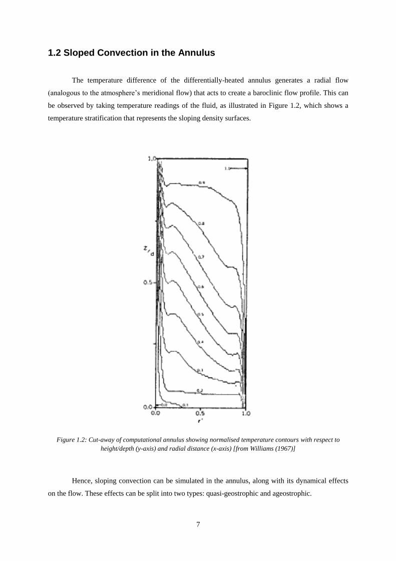
The temperature difference of the differentially-heated annulus generates a radial flow
(analogous to the atmosphere‟s meridional flow) that acts to create a baroclinic flow profile. This can
be observed by taking temperature readings of the fluid, as illustrated in Figure 1.2, which shows a
temperature stratification that represents the sloping density surfaces.
Figure 1.2: Cut-away of computational annulus showing normalised temperature contours with respect to
height/depth (y-axis) and radial distance (x-axis) [from Williams (1967)]
Hence, sloping convection can be simulated in the annulus, along with its dynamical effects
on the flow. These effects can be split into two types: quasi-geostrophic and ageostrophic.

8
The quasi-geostrophic approximation assumes that the Rossby Number (the ratio of inertial
acceleration to Coriolis acceleration, explained in the next chapter) is small but non-negligible,
allowing derivation of the quasi-geostrophic potential vorticity which, in terms of the streamfunction
, can be written in the form:
(1.1)
where , and are the zonal, meridional and vertical directions respectively, and (the planetary
vorticity, which can be omitted due to being constant) are from the beta-plane approximation to the
Coriolis parameter and is the buoyancy frequency. This is a very useful result,
allowing a single unknown, , to describe the entire motion of the system. As such, quasi-geostrophic
models are very common, often employed even when the approximation starts to break down, for
instance when topography becomes large enough.
Quasi-geostrophic dynamics are low-order phenomena, achievable by simple numerical
models with only a small number of modes. Ageostrophic dynamics, on the other hand, require either
high-resolution computational models or laboratory studies to be observed. In the next two sections,
the most important occurrences of both will be briefly introduced and discussed.
1.2.1 Quasi-Geostrophic Dynamics
The most important low-order effect of sloping convection in an annulus is the advent of
baroclinic waves. At low rotation rates, flow structure is uniform in the azimuthal direction1. Hide and
Mason (1975) refer to this region as „axisymmetric‟. When the rotation rate surpasses a certain critical
value, however, the flow becomes „non-axisymmetric‟ and azimuthal variation is introduced in the
form of eddies. The number of eddies that occur increases with increased rotation (and/or thermal
forcing) until a second critical value is reached whereupon the structure becomes dominated by chaos.
These eddies are baroclinic waves, and are illustrated in Figure 1.3.
1 Andrews (2000) notes the similarity to the Hadley Cell circulation.

9
Figure 1.3: Streakline images illustrating how the flow structure develops as rotation rate increases - a.)
rads-1
, b.) rads-1
c.) rads-1
d.) rads-1
e.) rads-1
f.)
rads-1
[from Hide and Mason (1975)]
Each flow structure is named after the „period‟ of the waves, with (b) referred to as
wavenumber-2, (c) as wavenumber-3, (d) as wavenumber-5, and so-on. Furthermore, the waves can
be either stationary or drifting, depending on whether they oscillate at the same rate as the annulus or
not, and either vacillating or steady, depending on whether the eddies maintain a constant size and
shape or not. Amplitude vacillation is where the eddies grow or shrink in the radial direction over
time, and structural vacillation (which occurs with more intense forcing) is where the eddies change in
appearance, for example becoming unevenly spaced around the annulus. These terms will become
important in describing the results of this thesis‟ experiments.

10
The transitions between baroclinic wave regimes lead to another aspect of sloping convection:
temporal period-doubling amplitude vacillation. This phenomenon was investigated by Young and
Read (2008), in a computational study of a differentially-heated annulus. Period-doubling amplitude
vacillation has been noted in other annulus studies, such as in Hart (1985) where the forcing is
generated by differential rotation, but Young and Read present the first case of the regime occurring
in a purely thermal forced annulus. As the name suggests, the regime was defined as a wavenumber-2
amplitude vacillation that undergoes period-doubling bifurcations until chaos is reached. The
bifurcations were observed as multiple or aperiodic loops in delay coordinate reconstructions, with the
notation of 2AV-d1 for a single loop (this can be differentiated from a normal wavenumber-2
amplitude vacillation, referred to as 2AV, by the width of the attractor), up to 2AV-dh for higher
order aperiodic states.
The authors suggest the possibility of a bifurcation sequence (shown in Figure 1.4), where, by
increasing the Taylor Number, the flow gains periodicity at state 2AV-d1, bifurcates to 2AV-d2,
continues bifurcating to the chaotic state 2AV-dh (A), oscillates between 2AV-d3 and 2AV-dh (B),
settles on 2AV-d3 (C), returns to 2AV-d1 (D), before finally losing periodicity again.
Figure 1.4: Possible bifurcation sequence of wavenumber-2 regime [from Young and Read (2008)]

11
As these bifurcations have not yet been observed in a physical differentially-heated annulus,
part of the first year of this thesis will consist of a laboratory study, attempting to replicate the
proposed period-doubling sequence. The objective of the study will be to perform experiments in the
same parameter space as Young and Read (2008), verifying the existence of the bifurcations by
creating delay coordinate reconstructions from velocity data. From that point, further investigations
can be made, examining the links between period-doubling and such areas as Rayleigh-Bénard
convection and turbulence (as discussed in Gollub and Benson (1980), for example).
A secondary objective of this study will be to gain a working knowledge of the experimental
rig. By using an unmodified rig to verify the findings of a recent numerical investigation, the results
gathered should improve the approach for the subsequent years of research. Hence, after the
conclusion of the study, it is hoped that the understanding of the annulus obtained will clarify how
best to re-design the equipment arrangement for optimal performance.
1.2.2 Ageostrophic Dynamics
Inertia-gravity waves are amongst the most notable examples of the ageostrophic effects of
sloping convection. They are ageostrophic as they form within the thermal boundary layer of the
annulus, which cannot be modelled by quasi-geostrophic theory. Whilst inertia-gravity waves have a
shorter period and are less apparent in annulus experiments than baroclinic waves, in the atmosphere
they have recently been linked to both the occurrence of turbulence2 and transitions between
wavenumbers3. Jacoby et al (2010) also note that the momentum transport they provide is essential to
the understanding of the atmospheric circulation. Despite the obvious importance of inertia-gravity
waves, their mechanism of generation in the annulus remains unknown.
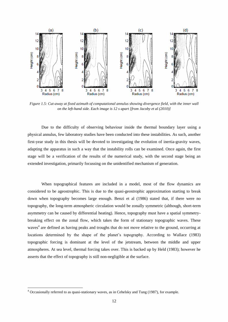
In the annulus, Jacoby et al conducted a numerical study, finding small-scale “overturning
events” in the divergence and temperature fields within the boundary layer at the inner wall. These
downwards-propagating features were found to drift in phase azimuthally with the baroclinic waves of
the main flow. Due to the periodic nature of these structures, they were named „instability rolls‟,
pictured in Figure 1.5. The rolls were put forward by Jacoby et al as a possible cause of inertia-gravity
waves in the annulus.
2 By Knox, McCann and Williams (2008).
3 By Williams, Read and Haine (2003).
12
Figure 1.5: Cut-away at fixed azimuth of computational annulus showing divergence field, with the inner wall
on the left-hand side. Each image is 12 s apart [from Jacoby et al (2010)]
Due to the difficulty of observing behaviour inside the thermal boundary layer using a
physical annulus, few laboratory studies have been conducted into these instabilities. As such, another
first-year study in this thesis will be devoted to investigating the evolution of inertia-gravity waves,
adapting the apparatus in such a way that the instability rolls can be examined. Once again, the first
stage will be a verification of the results of the numerical study, with the second stage being an
extended investigation, primarily focussing on the unidentified mechanism of generation.
When topographical features are included in a model, most of the flow dynamics are
considered to be ageostrophic. This is due to the quasi-geostrophic approximation starting to break
down when topography becomes large enough. Benzi et al (1986) stated that, if there were no
topography, the long-term atmospheric circulation would be zonally symmetric (although, short-term
asymmetry can be caused by differential heating). Hence, topography must have a spatial symmetry-
breaking effect on the zonal flow, which takes the form of stationary topographic waves. These
waves4 are defined as having peaks and troughs that do not move relative to the ground, occurring at
locations determined by the shape of the planet‟s topography. According to Wallace (1983)
topographic forcing is dominant at the level of the jetstream, between the middle and upper
atmospheres. At sea level, thermal forcing takes over. This is backed up by Held (1983); however he
asserts that the effect of topography is still non-negligible at the surface.
4 Occasionally referred to as quasi-stationary waves, as in Cehelsky and Tung (1987), for example.

13
Another influence of topography on the atmosphere is the formation of flow regimes, as
explained by Charney and DeVore (1979). Topographical forcing can lead to the development of
either a „low index‟ flow or a „high index‟ flow. The former state (also known as „blocking‟) is
defined as having “a strong wave component and a weaker zonal component locked close to linear
resonance”; this locking is caused by the non-linear interactions of the topography with the zonal
flow. The latter state (also known as „zonal‟ flow) has “a weak wave component and a stronger zonal
component much further from linear resonance”. Both states are stable (sometimes also referred to as
metastable or quasi-stable), giving rise to the concept of multiple equilibria. Transitions between the
two states are forced by baroclinic instabilities of the topographic waves.
As topography is so important to atmospheric circulation (with the above only giving a few
effects), a topographic study will form the major part of this thesis, with an experimental investigation
beginning in the second year. More impacts of topography will be discussed in Chapter 5, along with
unresolved questions found from a review of the literature on the topic. It is the answers to these
questions that will determine the course of the topographic study, as well as the precise nature of the
experiments to be carried out.
1.3 Summary
The format that this report will take is as follows. Firstly, Chapter 2 will be a detailed account
of the experimental apparatus that this project will utilise, including the methodology that will be
employed and explanations of the experiments to be carried out in the first year of study. The chapter
will also contain a short explanation of some of the key dimensionless numbers needed to describe the
parameter space. Next, Chapter 3 will provide the results of these experiments, and contain initial
observations made. This will be followed by a discussion, Chapter 4, examining the progress of the
first year of study and suggesting outstanding issues for later investigation. Chapter 5 will then move
on to the planned research on topographic effects to be undertaken in the second and third years of the
thesis, describing what unresolved questions about the effects of topography on the atmospheric
circulation remain to be investigated, what laboratory work has already been carried out on the subject
and how the current apparatus can be altered to investigate these effects. Chapter 6 will consolidate all
the outstanding issues from the preliminary conclusions and the plan for adapting the annulus for
topographic investigation in order to create an outline for the aims and objectives for the next two
years of the thesis. In addition, a timeline of work until the end of the project will be established and
justified. Lastly, Chapter 7 gives a list of the various references used to assemble this report.
14
Chapter 2
Experimental Arrangement
This chapter will first explain the apparatus available for this project‟s investigation, split up
into the experimental equipment itself and all the hardware and software needed to actually generate
results. Descriptions of the both the basic arrangement used to investigate the bifurcation phenomena
and the slightly altered arrangement used to investigate inertia-gravity waves will be given. The next
section will detail the process of how everything was put together, and the final section will describe
how the equipment will be employed to achieve meaningful solutions to the problems posed in the
previous chapter. Firstly, however, a brief introduction to some of the more relevant dimensionless
numbers will be provided, in order to give context to the parameter space under investigation.
2.1 Non-dimensional Numbers
Whilst the flow of the atmospheric circulation is extremely complicated, for typical annuli
experiments (and computational annulus models) the entire system can be reduced to two
dimensionless numbers which fully describe parameter space. Firstly, the Taylor Number is defined
as:
(2.1)
where is the characteristic length scale and ν is the kinematic viscosity. The Coriolis Parameter, ,
also known as the Coriolis Frequency, describes the effect of the planetary rotation ( ) depending on
latitude ( ) and is found using the equation:
(2.2)
For an annulus experiment, is taken to be 90°, and the Taylor Number can be adapted to the form:
(2.3)
where is the inner radius, is the outer radius and is the height of the annulus and is the rate of
rotation of the fluid. Roughly, the Taylor Number gives the ratio of the Coriolis forces (the
15
numerator) to the viscous forces (the denominator) acting upon a fluid. A large value implies a less
stable flow, with circulation tending toward higher dominant wavenumbers and the irregular regime.
Secondly, the Rossby Number is defined as:
(2.4)
where is the characteristic velocity scale of the fluid. For an annulus experiment, this can be
adapted into the Thermal Rossby Number (sometimes also known as the Hide Number, hereafter
simply „the Rossby Number‟) which takes the form:
(2.5)
where is the thermal expansion coefficient, is the gravitational acceleration and is the
temperature difference. Roughly, the Rossby Number gives the ratio of the inertial forces (the
numerator) to the Coriolis forces (the denominator) acting upon a fluid. At large values the
geostrophic approximation (explained in the next chapter) begins to break down, leading to Houghton
(2002) to refer to the Rossby Number as a “measure of the validity of the geostrophic approximation”.
As most of the quantities are assumed (or fixed) to be constant, the Taylor Number can be
simplified to being proportional to , and the Rossby Number can be simplified to being
proportional to
. For an annulus experiment (or similar) the rotation rate and the temperature
difference are the main sources of control, hence, these two dimensionless numbers can be taken to
fully describe the parameter space that the experiments take place within, as noted by Hide and Mason
(1975) in their pioneering study of the annulus.
For the study of inertia-gravity waves, a third dimensionless number becomes important – the
Prandtl Number, defined as:
(2.6)
where is the thermal diffusivity. The Prandtl Number gives the ratio of the viscous diffusion (the
numerator) to the thermal diffusion (the denominator) acting upon a fluid. White (2008) gives the
alternate definition of the ratio between dissipation and conduction. In annulus experiments, the
Prandtl Number is dependent on the working fluid employed. There exists a critical value of roughly
12 (Randriamampianina, private communication) where the inertia-gravity waves change from being
stationary waves to drifting waves. A further review of the importance of the Prandtl Number can be
found in Fein and Pfeffer (1976) or Randriamampianina et al (2006).
16
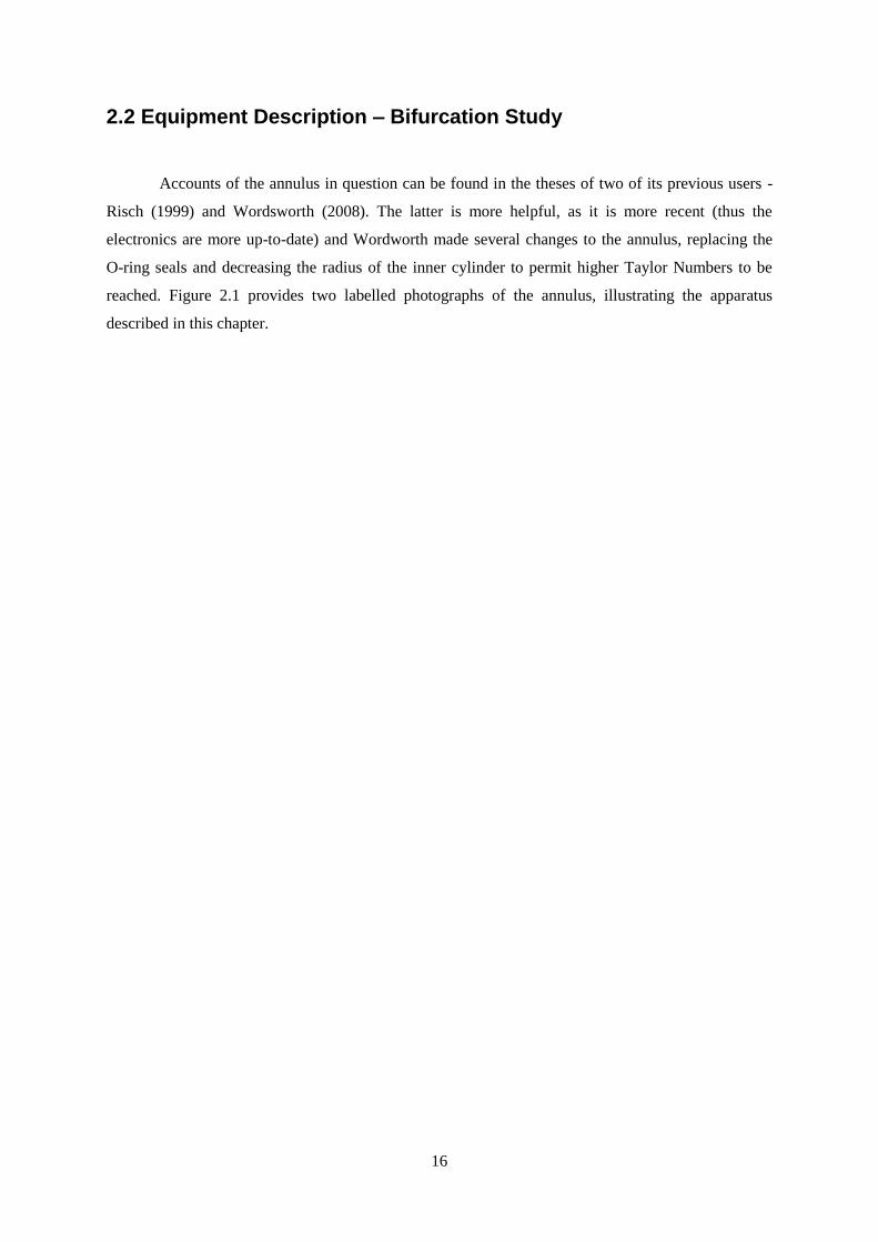
2.2 Equipment Description – Bifurcation Study
Accounts of the annulus in question can be found in the theses of two of its previous users -
Risch (1999) and Wordsworth (2008). The latter is more helpful, as it is more recent (thus the
electronics are more up-to-date) and Wordworth made several changes to the annulus, replacing the
O-ring seals and decreasing the radius of the inner cylinder to permit higher Taylor Numbers to be
reached. Figure 2.1 provides two labelled photographs of the annulus, illustrating the apparatus
described in this chapter.

17
a.)
b.)
Figure 2.1: Annotated photographs of the annulus from two different sides, with apparatus arranged for the
bifurcation study.
18
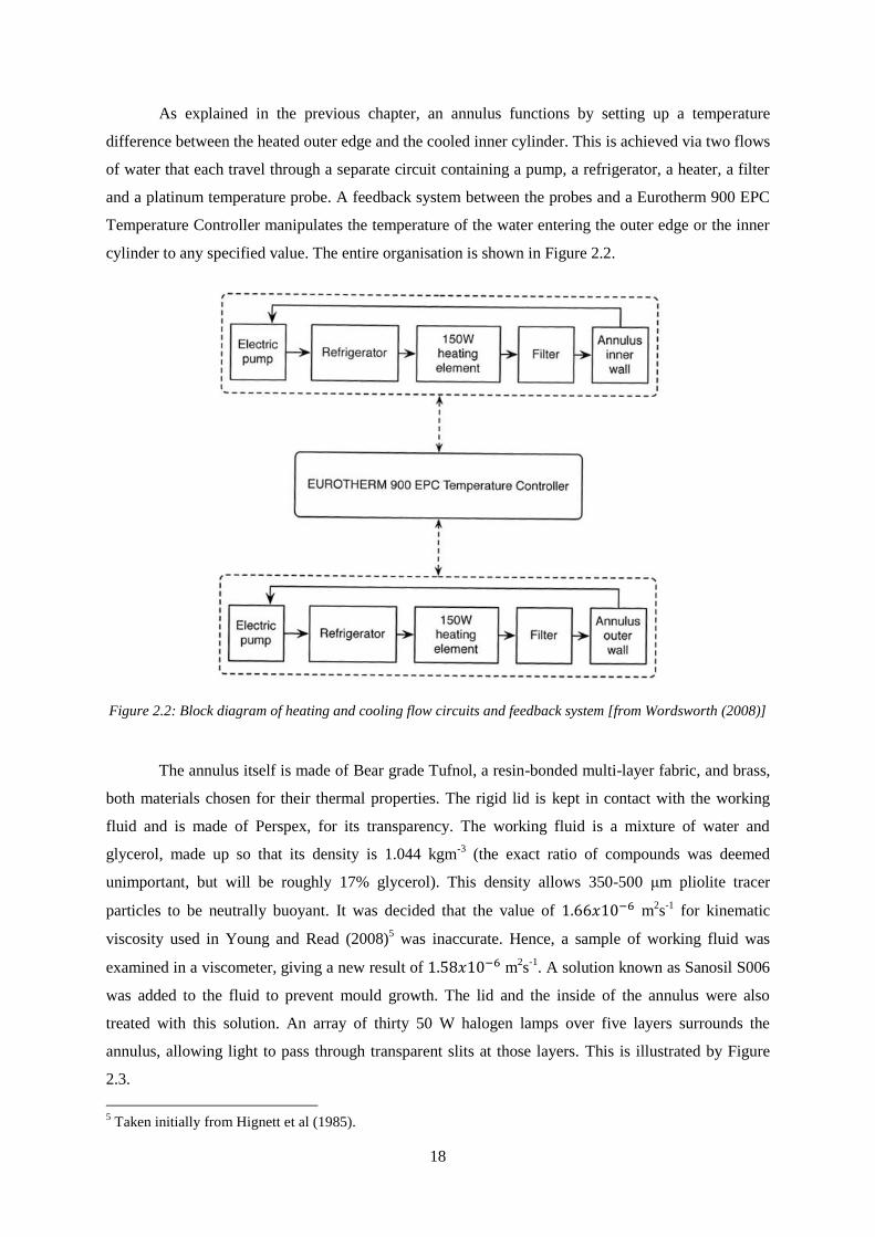
As explained in the previous chapter, an annulus functions by setting up a temperature
difference between the heated outer edge and the cooled inner cylinder. This is achieved via two flows
of water that each travel through a separate circuit containing a pump, a refrigerator, a heater, a filter
and a platinum temperature probe. A feedback system between the probes and a Eurotherm 900 EPC
Temperature Controller manipulates the temperature of the water entering the outer edge or the inner
cylinder to any specified value. The entire organisation is shown in Figure 2.2.
Figure 2.2: Block diagram of heating and cooling flow circuits and feedback system [from Wordsworth (2008)]
The annulus itself is made of Bear grade Tufnol, a resin-bonded multi-layer fabric, and brass,
both materials chosen for their thermal properties. The rigid lid is kept in contact with the working
fluid and is made of Perspex, for its transparency. The working fluid is a mixture of water and
glycerol, made up so that its density is 1.044 kgm-3
(the exact ratio of compounds was deemed
unimportant, but will be roughly 17% glycerol). This density allows 350-500 μm pliolite tracer
particles to be neutrally buoyant. It was decided that the value of m2s
-1 for kinematic
viscosity used in Young and Read (2008)5 was inaccurate. Hence, a sample of working fluid was
examined in a viscometer, giving a new result of m2s
-1. A solution known as Sanosil S006
was added to the fluid to prevent mould growth. The lid and the inside of the annulus were also
treated with this solution. An array of thirty 50 W halogen lamps over five layers surrounds the
annulus, allowing light to pass through transparent slits at those layers. This is illustrated by Figure
2.3.
5 Taken initially from Hignett et al (1985).

19
Figure 2.3: Schematic of the lighting array and heating system in side view [adapted from Wordsworth (2008)]
Due to the nature of the halogen lamps, which are very prone to overheating and thus also
causing an additional heat source on the outer edge, three large electric fans were attached to the
lighting array. An electronic control box controls which of the five layers is illuminated at a time, with
an option for an automatic shift between them at a variable rate. A camera is mounted above the
annulus on a tripod-shaped superstructure, with a cone blocking all outside light between it and the
Perspex lid. With this arrangement, the camera can see the motion of the tracer particles, and thus the
flow structure, at any one of the five levels in Figure 2.3. By switching quickly between the layers, the
vertical structure can also be resolved.
The annulus to be used is a larger model than the standard, as it was designed for use at high
Taylor Numbers. Its dimensions, as well as several other relevant experimental parameters, are given
in Table 2.1.
Radius of Inner Cylinder a 4.5 cm
Radius of Outer Cylinder b 14.3 cm
Depth of Annulus d 26.5 cm
Kinematic Viscosity of Water νw m2s
-1
Thermal Expansion Coefficient of Water αw K-1
Density of Water-Glycerol Mixture ρg 1.044 kgm-3
Kinematic Viscosity of Water-Glycerol Mixture νg m2s
-1
Thermal Expansion Coefficient of Water-Glycerol Mixture αg K-1
Table 2.1: Important experimental parameters
20
2.2.1 Data Acquisition
In deference to previous set-ups, a Firewire (type: DFK 31BF03) camera was selected for
taking visual results, due to its high picture quality and supposed simplicity of connection with a Mac
Mini computer. The Mac Mini, a recent model, is small and light enough to be mounted to the rotating
frame, and saved the images and movies to a 500 Gb Seagate Hard Drive. A Local Area Network
(LAN) was set up to allow it to communicate with a second computer in the laboratory frame. This
stationary computer is known as the „base station‟. In addition to this digital signal, an analogue signal
was also taken from the camera via a slip-ring to a specialised console (a PC and several monitors
attached to a SVHS video recorder). It was hoped that both signals could be achieved simultaneously
thanks to a Canopus ADVC 110 Analogue/Digital Converter attached to the Mac Mini.
In terms of software, the free TightVNC (Virtual Network Client) package allows the base
station to remotely control the Mac Mini, and therefore the camera functions. The specialised console
used a program known as Digimage to create streak-line images and movies from the analogue signal.
These results give an idea of the type of flow at a given point: which wavenumber most resembles the
motion, whether the waves are stationary or drifting and whether any kind of vacillation is observed.
However, due to the noise of the signal and the age of the analogue equipment, these results are of no
use for further analysis. The digital signal, on the other hand, goes through a slightly more
complicated process. It is picked up on the base station by a software program called BTV Pro, which
takes movies of the flow in motion and makes hundreds of frame-by-frame images from them. BTV
Pro also ensures the gain of the camera is constant, so that each image occurs under the same
conditions. These images are then transferred to a MATLAB program called Coriolis, an example of
Correlation Image Velocimetry (CIV) – an iterative algorithm that tracks the translation, rotation and
shear motion of the tracer particles. From this information, CIV creates a velocity vector field of the
flow, with the option of manually removing any false readings. Modal analysis of the vector field
should prove extremely important for detailed examination of the fluid structure, including the ability
to create delay coordinate reconstructions, for use in the investigation of Young and Read‟s (2008)
bifurcations.

21
2.3 Inertia-Gravity Wave Study Arrangement
For the study of inertia-gravity waves it was necessary to examine the fluid motion within the
thermal boundary layer, hence the experimental arrangement required a few modifications. The most
notable of these was an alternative visualisation method, created by removing the tracer particles and
injecting a solution of Fluorescein sodium (a luminous green dye) directly into the boundary layer via
a needle held very close to the inner wall of the annulus. The amount of dye added was controlled
using a remote-operated mechanical syringe pump. To improve the clarity of the images obtained, one
half of the inner wall was painted white. The whole arrangement is shown in Figure 2.4.
Figure 2.4: Annotated photograph of dye injection system
22
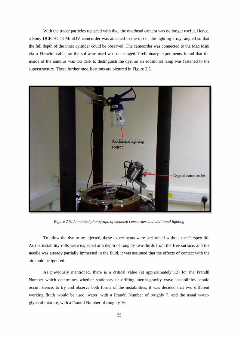
With the tracer particles replaced with dye, the overhead camera was no longer useful. Hence,
a Sony DCR-HC44 MiniDV camcorder was attached to the top of the lighting array, angled so that
the full depth of the inner cylinder could be observed. The camcorder was connected to the Mac Mini
via a Firewire cable, so the software used was unchanged. Preliminary experiments found that the
inside of the annulus was too dark to distinguish the dye, so an additional lamp was fastened to the
superstructure. These further modifications are pictured in Figure 2.5.
Figure 2.5: Annotated photograph of mounted camcorder and additional lighting
To allow the dye to be injected, these experiments were performed without the Perspex lid.
As the instability rolls were expected at a depth of roughly two-thirds from the free surface, and the
needle was already partially immersed in the fluid, it was assumed that the effects of contact with the
air could be ignored.
As previously mentioned, there is a critical value (at approximately 12) for the Prandtl
Number which determines whether stationary or drifting inertia-gravity wave instabilities should
occur. Hence, to try and observe both forms of the instabilities, it was decided that two different
working fluids would be used: water, with a Prandtl Number of roughly 7, and the usual water-
glycerol mixture, with a Prandtl Number of roughly 16.

23
2.4 Process of Re-building and Issues
When the project began, the apparatus had been taken apart to make space for other
experiments. Hence, the major task of the first year of work was to restore the equipment to such a
point where experiments could be carried out. Before any of this could begin, however, the turntable
was tested for an inherent „wobble‟ noted by Wordsworth (2008). A bowl of water was placed in the
center of the turntable, to see if any asymmetric ripples could be observed. As none were found, it was
decided that the reported vibration must have been due to a section of plumbing rubbing against the
structure as it rotated. When the re-build was complete, a second vibration test was carried out, once
again finding the „wobble‟ to be negligible.
To make sure the annulus was positioned exactly in the center of the turntable, an optical
cathetometer (also known as a tracking telescope) was employed. Warping of the wooden annulus
base caused a small deviation to the rotation, measured by a Baty Dial Test Indicator to have a
maximum of roughly 1.5 mm. As this deviation was confined to the base, not the outer or inner
cylinders, this was judged to be negligible.
Once all the components were fixed in the correct location, the process of connecting up the
plumbing could begin. All the previous pipes and insulation had been lost or discarded when the
apparatus was taken apart, so the entire water system was replaced with new material. During this
time various leaks were repaired as well as possible and the impellor for the outer cylinder pump was
replaced. The electronics were next to be installed, with the camera, Mac Mini and hard drive attached
to the superstructure and all those devices (and the fans, lights etc) were connected to the mains via a
slip ring. Lastly, the Firewire camera needed a different attachment to the one used by Wordsworth
(2008), so a new aluminium bracket was designed and built. Unfortunately, the Firewire camera and
the analogue/digital converter were found to be incompatible so, at this stage, only one of the two
signals can be obtained at a time.
2.5 Methodology – Bifurcation Study
Young and Read (2008) highlighted their results at four points of given Taylor and Rossby
Numbers, illustrated as A, B, C and D by Figure 2.6. Though it has been noted6 that transitions will
occur in different locations for different annuli, these points should form an excellent place start in the
search for the bifurcation sequence.
6 By Hignett et al (1985), for example.

24
Figure 2.6: Non-dimensional location of the four major results of Young and Read (2008).
This project‟s annulus is significantly larger than that used by Hignett et al (1985) and Young
and Read (2008). This difference is given in Figure 2.7.
(a) (b)
Figure 2.7: Annulus comparison between (a) Young and Read (2008) and (b) the current study [from
Wordsworth (2008)]

25
As the current annulus is larger, a, b and d will all change, altering the Taylor and Rossby
Numbers and requiring new values for rotation rates and temperature differences to achieve the same
dimensionless numbers, and, in turn, points in parameter space. The calculation of points A, B, C and
D from Figure 2.6 with this project‟s apparatus is shown in Table 2.2.
A B C D
Taylor Number 3.55x10⁶ 3.73x10
6 3.83x10
6 4.04x10
6
Rossby Number 1.756 1.752 1.754 1.755
Calculated Rotation Rate (rads-1
) 0.255 0.261 0.265 0.272
Calculated Temperature Difference (K) 1.335 1.140 1.440 1.518 Table 2.2: Calculation of rotation rates and temperature differences from Young and Read’s highlighted results
(calculated values to 3 d.p.)
Unfortunately preliminary experiments found that, at these low rotation rates and temperature
differences, the evolved wave structure was too weak to maintain the floating tracer, and most of the
particles fell to the bottom of the annulus. As such, it was decided to investigate more intense regimes
for evidence of period doubling. To this end, and to additionally determine how to achieve the highest
quality of results, a great number of different flows were studied. The most important of these are
given below:
An attempt to find the temperature difference at which the particle visualisation technique
becomes viable, with differences of 1, 2, 3, 4, 5, 6 and 7 K at a rotation rate of 0.65 rads-1
.
High Taylor Number flows at rotation rates of 2.45, 2.75 and 3 rads-1
at a temperature
difference of 5 K, in order to investigate a chaotic, unstable regime with high forcing.
Low Taylor Number flows at rotation rates of 0.6, 0.7, 0.8 and 0.9 rads-1
at a temperature
difference of 3 K, in order to search for bifurcations in an area of moderate forcing.
A scan7 with rotation rate increasing at 0.2 rads
-1 intervals from 1 to 1.6 rads
-1 at a
temperature difference of 3 K, in order to observe the effects of hysteresis.
A scan with rotation rate decreasing at 0.2 rads-1
intervals from 1.6 to 1 rads-1
at a
temperature difference of 3 K, in order to further observe the effects of hysteresis.
To ensure particle saturation, the annulus was sped up to an arbitrary high rotation rate before
being slowed to the relevant speed under examination. The apparatus was then left for one hour to
allow the fluid to achieve solid-body rotation and to allow the wave structure to become fully
baroclinic. After this point, results were taken over the course of 60 minutes. Due to issues with the
illumination from the lighting array, all readings were taken at the brightest height – level 2, at 17.4
cm above the base.
7 A „scan‟ implies that the fluid was not returned to rest between readings.

26
To begin with, only the analogue signal will be employed, as the real-time streakline images
generated by Digimage will allow for easier observation of the bifurcation phenomena. Once evidence
of the bifurcations is found, the focus will shift to the digital signal, and the same parameters will be
used. In this way, an array of images will be taken via BTV Pro, allowing CIV to create velocity
vector diagrams of the flow. Modal analysis of this data can then be used to produce delay coordinate
reconstructions, as the shape of the attractor is the best illustration of period doubling.
2.6 Methodology – Inertia-Gravity Wave Study
Whilst the bifurcation study was defined by the attempt to replicate the work of Young and
Read (2008), the study of inertia-gravity waves was conducted under the guidance of Peter Read,
Wolf-Gerrit Früh and Antony Randriamampianina. The latter suggested a starting place in parameter
space of 1.3 rads-1
rotation rate and 2 K temperature difference for the water-glycerol mixture
experiment, analogous to 1 rads-1
rotation rate and 2 K temperature difference for the water
experiment. From this point, two investigations could be launched: one into the effects of reducing the
rotation rate, the other into the effects of increasing the temperature difference.
For the water experiment this meant that nine separate readings were taken, with three
different rotation rates of 0.6, 0.8 and 1 rads-1
and three different temperature differences of 2, 5 and
10 K. Due the necessity of having to replace the fluid every few readings because of dye saturation, it
was decided that only one of the two investigations would be carried out with the water-glycerol
mixture. Preliminary experiments suggested that the reduction in rotation rate would be more fruitful,
due to the higher clarity of the images taken at the lowest temperature difference. As such, the water-
glycerol mixture experiment took only three readings, with three different rotation rates of 0.9, 1.1
and 1.3 rads-1
, all at the same temperature difference of 2 K.
In the same way as for the bifurcation study, the annulus was left for one hour after being
sped up to the required rotation rate (there was no need for particle saturation) to allow for solid-body
rotation and hence a stable thermal boundary layer. Due to the short lifetime of the tracer dye, results
were taken over a period of 5 minutes.

27
Chapter 3
Results
The results of both the bifurcation study and the inertia-gravity wave study are contained
within this chapter. More detail on the presented Figures will be explained in the introduction to each
section. After each study, a short analysis will be given, describing what is observed and noting any
trends discovered. For convenience, a sample regime diagram is provided in Figure 3.1, showing the
locations of both the proposed bifurcation sequence and the experiments of this study.
Figure 3.1: Regime diagram with locations of Increasing Temperature Difference (red), Low Taylor Number
(yellow) and High Taylor Number (green) experiments, along with the proposed bifurcation sequence (blue).
Individual readings are not shown for sake of clarity [originally from Hignett et al (1985); adapted from
Wordsworth (2008)]
28
3.1 Bifurcation Study
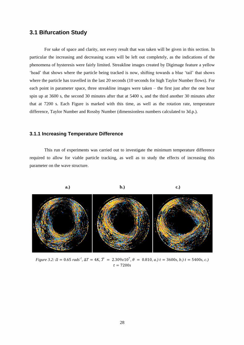
For sake of space and clarity, not every result that was taken will be given in this section. In
particular the increasing and decreasing scans will be left out completely, as the indications of the
phenomena of hysteresis were fairly limited. Streakline images created by Digimage feature a yellow
„head‟ that shows where the particle being tracked is now, shifting towards a blue „tail‟ that shows
where the particle has travelled in the last 20 seconds (10 seconds for high Taylor Number flows). For
each point in parameter space, three streakline images were taken – the first just after the one hour
spin up at 3600 s, the second 30 minutes after that at 5400 s, and the third another 30 minutes after
that at 7200 s. Each Figure is marked with this time, as well as the rotation rate, temperature
difference, Taylor Number and Rossby Number (dimensionless numbers calculated to 3d.p.).
3.1.1 Increasing Temperature Difference
This run of experiments was carried out to investigate the minimum temperature difference
required to allow for viable particle tracking, as well as to study the effects of increasing this
parameter on the wave structure.
a.) b.) c.)
Figure 3.2: rads-1
, K, , , a.) s, b.) s, c.)
s
29
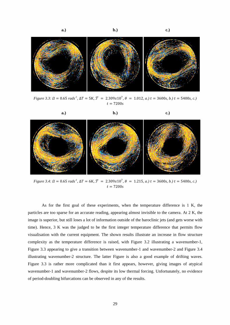
a.) b.) c.)
Figure 3.3: rads-1
, K, , , a.) s, b.) s, c.)
s
a.) b.) c.)
Figure 3.4: rads-1
, K, , , a.) s, b.) s, c.)
s
As for the first goal of these experiments, when the temperature difference is 1 K, the
particles are too sparse for an accurate reading, appearing almost invisible to the camera. At 2 K, the
image is superior, but still loses a lot of information outside of the baroclinic jets (and gets worse with
time). Hence, 3 K was the judged to be the first integer temperature difference that permits flow
visualisation with the current equipment. The shown results illustrate an increase in flow structure
complexity as the temperature difference is raised, with Figure 3.2 illustrating a wavenumber-1,
Figure 3.3 appearing to give a transition between wavenumber-1 and wavenumber-2 and Figure 3.4
illustrating wavenumber-2 structure. The latter Figure is also a good example of drifting waves.
Figure 3.3 is rather more complicated than it first appears, however, giving images of atypical
wavenumber-1 and wavenumber-2 flows, despite its low thermal forcing. Unfortunately, no evidence
of period-doubling bifurcations can be observed in any of the results.
30
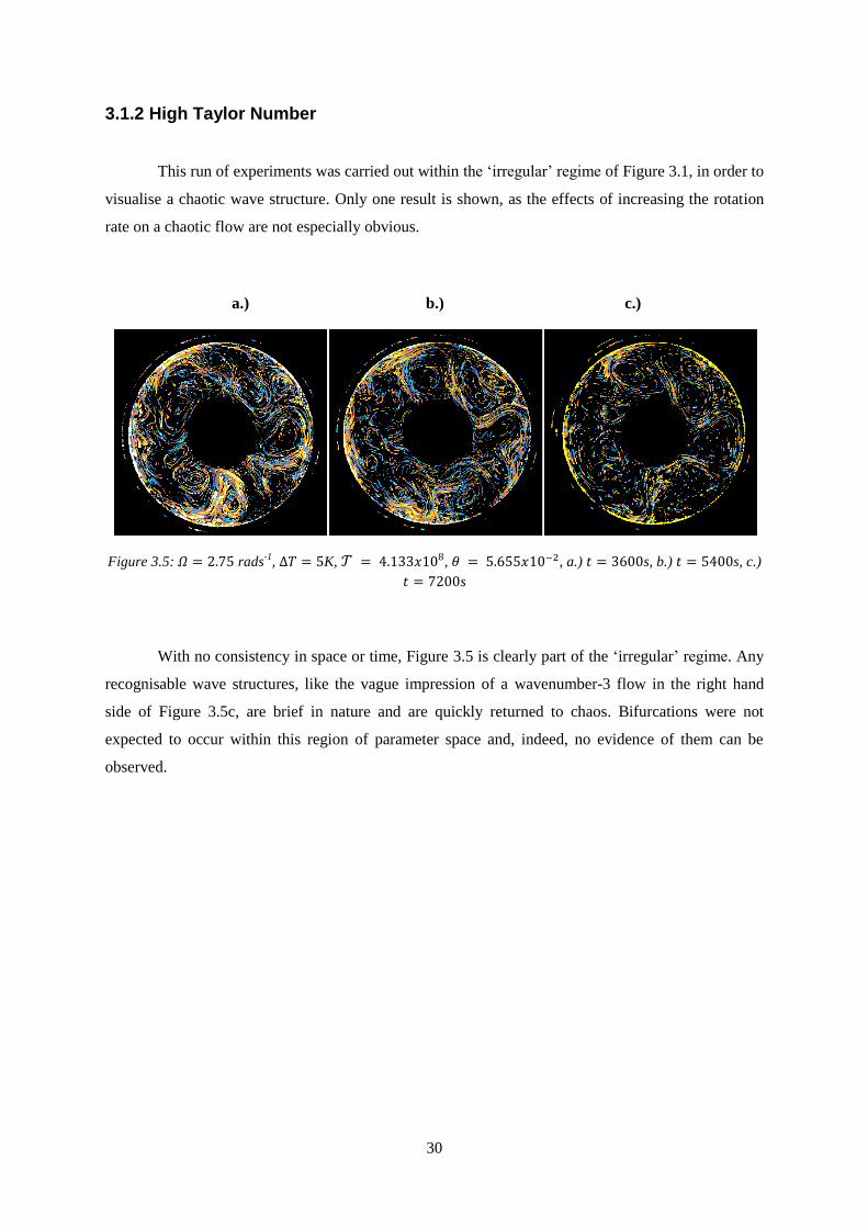
3.1.2 High Taylor Number
This run of experiments was carried out within the „irregular‟ regime of Figure 3.1, in order to
visualise a chaotic wave structure. Only one result is shown, as the effects of increasing the rotation
rate on a chaotic flow are not especially obvious.
a.) b.) c.)
Figure 3.5: rads-1
, K, , , a.) s, b.) s, c.)
s
With no consistency in space or time, Figure 3.5 is clearly part of the „irregular‟ regime. Any
recognisable wave structures, like the vague impression of a wavenumber-3 flow in the right hand
side of Figure 3.5c, are brief in nature and are quickly returned to chaos. Bifurcations were not
expected to occur within this region of parameter space and, indeed, no evidence of them can be
observed.

31
3.1.3 Low Taylor Number
This run of experiments was devised to attempt to get as close to the bifurcation sequence as
possible (see Figure 3.1), whilst still achieving adequate visualisation, by using the minimum
temperature difference of 3 K found previously.
a.) b.) c.)
Figure 3.6: rads-1
, K, , , a.) s, b.) s, c.)
s
a.) b.) c.)
Figure 3.7: rads-1
, K, , , a.) s, b.) s, c.)
s

32
a.) b.) c.)
Figure 3.8: rads-1
, K, , , a.) s, b.) s, c.)
s
a.) b.) c.)
Figure 3.9: rads-1
, K, , , a.) s, b.) s, c.)
s
Figures 3.6 to 3.9 describe a region much closer to where Young and Read (2008) observed
bifurcations in their experiments than the high Taylor Number flows. However, evidence of period-
doubling is still noticeably absent. Furthermore, once again Figure 3.1 suggests that these locations in
parameter space should be much steadier than what is observed, with only amplitude vacillation at
most. Instead, every experiment appears to structurally vacillate between wavenumbers to some
degree, and additional „wave lobes‟ are surprisingly common. For example, Figure 3.8a shows a
slightly skewed wavenumber-2, but 1800 s later in Figure 3.8b this has become a very atypical
wavenumber-4. Another 1800 s in Figure 3.8c and the wavenumber-2 structure has returned, but with
an obvious lobe at the top of the image. On the other hand, the results do show an increase in flow
structure complexity as rotation rate is raised, with Figure 3.6 being closest to wavenumber-1, Figures
3.7 and 3.8 being closest to wavenumber-2 and Figure 3.9 being closest to wavenumber-3 structure.

33
3.1.4 Vector Velocity Diagram
As no evidence of bifurcations was found at any point in parameter space, it was decided to
switch to the digital output signal anyway, and create an example vector velocity diagram of the flow.
The point in parameter space (a rotation rate of 0.65 rads-1
and 5 K temperature difference) was
chosen as the flow structure was amongst the most simple found, and yet had enough particle
saturation to produce a clear image.
A vector velocity diagram was created using CIV from two images with a time gap of one
second between, immediately following the hour long spin-up time (3600 s). Clearly anomalous or
„false‟ vectors flagged by the software were manually removed, and Figure 3.10 was produced.
Figure 3.10: Horizontal vector velocity diagram. Parameters as in Figure 3.3a

34
To further illustrate the flow structure, a background of a sample image from the annulus was
inverted and added to Figure 3.10, creating Figure 3.11. As CIV automatically „completes‟ the flow
field by inserting additional vectors where none were observed, a number of „imaginary vectors‟ lying
outside the bounds of the annulus were created. These have been removed from Figure 3.11.
Figure 3.11: Vector velocity diagram with inverse background, showing where flow structure occurs in annulus.
Parameters as in Figure 3.3a
Despite only being preliminary results, Figures 3.10 and 3.11 show extremely clear examples
of a wavenumber-3 structure.
35
3.2 Analysis – Bifurcation Study
Although a large number of points in parameter space have been investigated, no evidence for
bifurcations has been found so far. Referring to Figure 3.1, this is perhaps to be expected, as the
bifurcation sequence found by Young and Read (2008) takes place over a very small area and is still
an order of magnitude away in terms of Taylor Number from the nearest possible readings allowed for
by the visualisation technique. More surprisingly, steady flow regimes have proved equally elusive,
with some manner of structural vacillation occurring in all flows that were not fully irregular already
(Figure 3.5). This vacillation can be seen even at low rotation rates and temperature differences,
where previous studies8 have consistently found steady wavenumbers, and is especially clear in
Figure 3.3 where it can be observed that the flow first transitions between a wavenumber-2 and a
wavenumber-3 (a), then between a wavenumber-1 and a wavenumber-2 (b), and then seems to be
developing into a typical wavenumber-2 (c) over the course of the experiment. When the same
conditions were repeated to create the vector velocity diagram, a typical wavenumber-3 regime was
also found (Figures 3.10 and 3.11). It has been suggested that this is possibly due to the larger-than-
standard annulus in use having an increased Rayleigh Number, a dimensionless number dependent on
the on the scale of the gap between the inner and outer walls, defined for an annulus as:
(3.1)
This variation in Rayleigh Number could cause structural vacillation to occur at lower
rotation rates and temperature differences than would be the case in a more standard size of annulus
(Randriamampianina, private communication).
Alternatively, the additional wave-lobes and atypical structures may be due to another variety
of period-doubling: spatial period-doubling. The difference between this and the temporal period-
doubling of Young and Read (2008) is that the latter is primarily a route to chaos, whereas the former
is caused by transitional instabilities. As explained in Rabaud and Couder (1983) and Chomaz et al
(1988), who used films of soap trapped between two plates as their working fluids, spatial period-
doubling is generated by non-linear interactions between the main wave structure and its lesser
harmonics. For example, Figure 3.3b could be described as the superposition of a dominant
wavenumber-2 and a harmonic wavenumber-1 flow. This fits well with the findings of the soap
experiments, despite those period-doubling regimes being at much greater wavenumbers, due to the
differences in apparatus and approach.
8 Hignett et al (1985), for instance.
36
3.3 Inertia-Gravity Wave Study
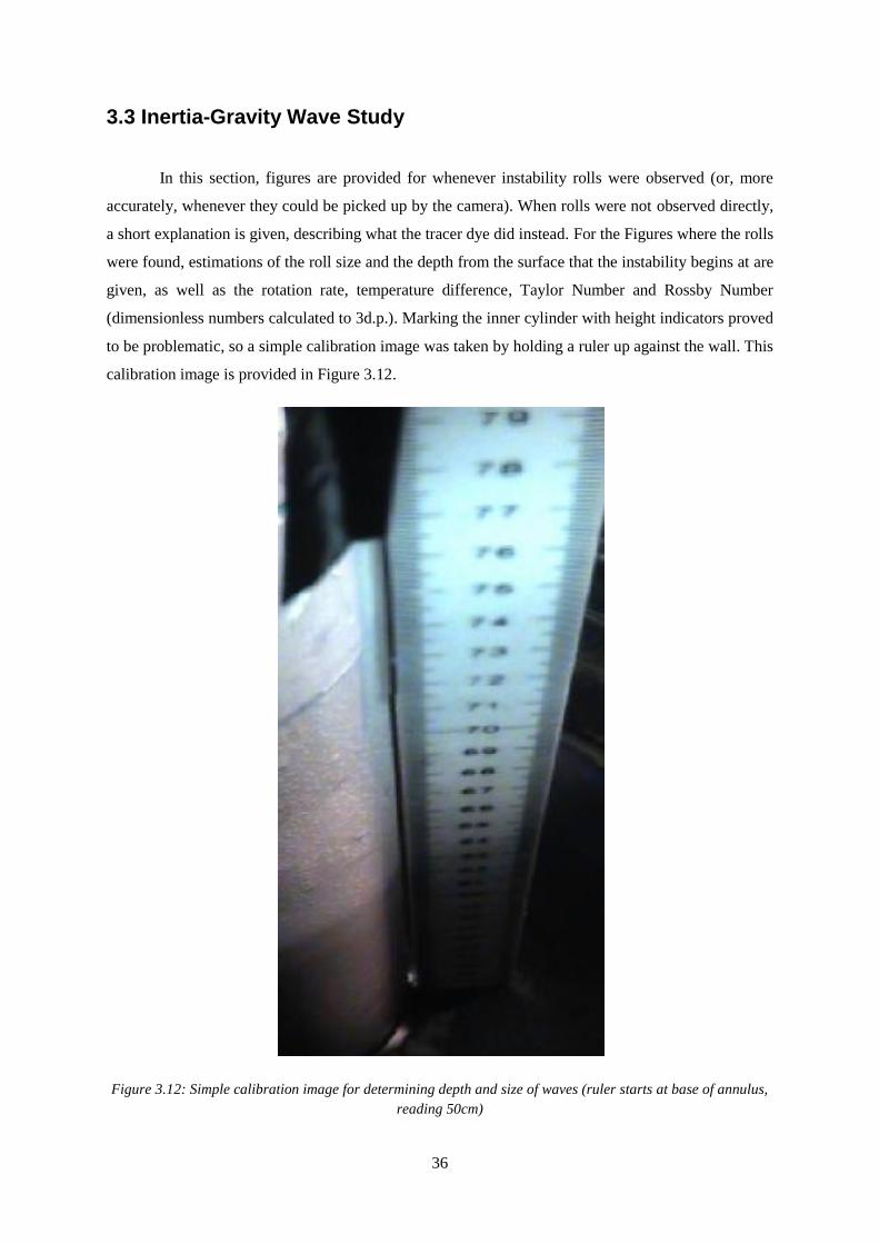
In this section, figures are provided for whenever instability rolls were observed (or, more
accurately, whenever they could be picked up by the camera). When rolls were not observed directly,
a short explanation is given, describing what the tracer dye did instead. For the Figures where the rolls
were found, estimations of the roll size and the depth from the surface that the instability begins at are
given, as well as the rotation rate, temperature difference, Taylor Number and Rossby Number
(dimensionless numbers calculated to 3d.p.). Marking the inner cylinder with height indicators proved
to be problematic, so a simple calibration image was taken by holding a ruler up against the wall. This
calibration image is provided in Figure 3.12.
Figure 3.12: Simple calibration image for determining depth and size of waves (ruler starts at base of annulus,
reading 50cm)

37
3.3.1 Water Experiments
For the first result only, three images will be given instead of one. This will allow for
visualisation of the formation and evolution of the instability roll. The other results (where the
instability is harder to observe) will show the final structure of the roll, equivalent to the third image,
permitting the magnitude of the wave within the thermal boundary layer to be measured. To indicate
the area where the roll is taking place, a blue box has been added to each image.
a.) b.) c.)
Figure 3.13: rads-1
, K, , , roll size (from c) = 10 cm, depth = 12 cm
The Figure 3.13a shows the tracer leaving the inner wall and beginning to form a roll. In
Figure 3.13b, the instability continues descending through the annulus, before the roll curves back and
re-joins the inner wall in Figure 3.13c.

38
a.) b.) c.)
Figure 3.14: a.) rads-1
, K, , , roll size = 4 cm, depth = 15 cm,
b.) rads-1
, K, , , roll size = 12 cm, depth = 13 cm,
c.) rads-1
, K, , , roll size = 5 cm, depth = 20 cm
In Figure 3.14, the tracer can be observed to follow the expected behaviour for a stationary
inertia-gravity wave, as described in Chapter 1. The dye within the thermal boundary layer descends
vertically before encountering an instability roll in the lower half of the annulus. After extending a
small amount towards the outer wall, the roll causes the tracer to return to the inner cylinder until the
flow reaches the base. Multiple rolls, on the other hand, were not observed under any conditions, even
in cases where the dye remained visible within the boundary layer all the way to the bottom.

39
At a rotation rate of 0.6 rads-1
and 2 K temperature difference no instability roll was observed
by camera or by eye. It was assumed that this implied that the rotational forcing at this rotation speed
was too small to allow inertia-gravity waves to form within the thermal boundary layer. In addition,
when the temperature difference was increased to 5 K, the result remained the same. This in turn
suggested that 0.6 rads-1
is too low a rotation rate for visible inertia-gravity waves, regardless of the
amount of thermal forcing.
In all experiments at the 10 K temperature difference, no viable readings were made. Due to
the large thermal forcing, the baroclinic waves were much more intense than in previous experiments,
and acted to drag the tracer away from the inner wall. The amount of dye that was able to remain
within the thermal boundary layer was too little to observe any instabilities. It is unknown, therefore,
whether inertia-gravity waves can occur under these conditions. The results of Jacoby et al (2010)
suggest that they should exist, but without further experiments this hypothesis would be impossible to
verify.
3.3.2 Water-Glycerol Mixture Experiments
Unfortunately, at this time, all experiments with a water-glycerol mixture as the working fluid
were unsuccessful. This was due to a new and foreseen problem: the relative density of the tracer dye.
Despite the Fluorescein sodium having been made up in a solution of water-glycerol with the same
density as the working fluid, when the dye was injected into the annulus it immediately floated to the
surface. It was suggested that this could be due to a small discrepancy in the density of the fluid
nearest the inner wall, where the cooling surface may fractionally increase the density of the
surrounding liquid. To compensate for this, the dye was re-created with slightly more glycerol in the
mixture, but this caused the opposite problem: the tracer descended rapidly down the boundary layer
and reached the base of the annulus before any instability roll could be set up. Due to time restraints,
any further experiments into inertia-gravity waves with water-glycerol mixture will have to form
future work in subsequent years of this thesis.

40
3.4 Analysis - Inertia-Gravity Wave Study
In the water experiments, stationary rolls were observed, as expected. However, with the lack
of the water-glycerol mixture experiments, no drifting rolls could be witnessed. By comparing Figures
3.13 and 3.14b (1 rads-1
) to Figures 3.14a and 3.14c (0.8 rads-1
), it can be observed that, as the rotation
rate decreases, the instability rolls get smaller and more difficult to see. Similarly, by comparing
Figures 3.13 and 3.14a (2 K) to Figures 3.14b and 3.14c (5 K), it can be observed that, as the
temperature difference increases, the rolls occur closer to the base of the annulus. Even through the
roll in Figure 3.14b begins at a slightly higher depth than the roll in Figure 3.14a, the former is much
larger, and terminates very close to the base of the annulus. The absence of multiple rolls is
surprising, but is possibly due to the secondary rolls either being too small to be seen, or occurring too
low in the annulus to be discernable from the dye encountering the base.

41
Chapter 4
Preliminary Conclusions
In this chapter the various results and observations of Chapter 3 will be examined in greater
detail, with a discussion on what has been learnt from both studies. A section will then highlight the
outstanding issues of the first-year experiments, both in terms of possible methods to observe
phenomena that were not encountered with the current arrangement and further extensions to the
studies to investigate other aspects of bifurcations and inertia-gravity waves.
4.1 Discussion – Bifurcation Study
The major conclusion of the bifurcation study is that, due to the large annulus in use,
structural vacillation is a regular occurrence at most points in the observed parameter space. This
indicates that the current position of investigation is too far from the bifurcation sequence (Figure
3.1). In addition, Young and Read‟s (2008) bifurcations were found to occur within the wavenumber-
2 amplitude vacillation region. Despite some results (Figure 3.4, for example) showing reasonably
steady drifting wavenumber-2 structures, the prevalence of structural vacillation in the rest of the
experiments meant that the location of this region remained elusive, let alone the tiny area within this
region containing the supposed bifurcation sequence. A further problem is that, if temperature
difference and rotation rate are reduced to get closer to the bifurcations, the weak baroclinic waves
evoked would not be enough to allow particles to saturate the flow and be visible. With the current
arrangement of annulus and visualisation technique, temporal period-doubling appears to be
impractical to investigate.
On the other hand, the results gathered bear some resemblance to spatial period-doubling was
discovered. This is an interesting phenomenon in its own right, despite having been observed in
laboratory research before, and further study could be achieved by carrying out more experiments in
the same parameter space, finding the limits of where spatial period-doubling occurs.
As a tertiary finding, above a temperature difference of 3 K it was established that the particle
tracking software could produce good quality images of vector velocities (Figures 3.10 and 3.11). The
visualisation equipment and software used are therefore clearly viable for results gathering in the
subsequent years of this thesis.

42
4.2 Discussion – Inertia-Gravity Wave Study
The inertia-gravity wave study was the notably more successful of the two investigations.
Instability rolls were observed in a laboratory setting, and a reasonable visualisation of the thermal
boundary layer structure was achieved (Figure 3.13). It was also found that decreasing the rotation
rate reduces the size of the instability rolls, whilst increasing the temperature difference causes the
rolls to occur at a greater depth, verifying the numerical results of Jacoby et al (2010). These findings
are only qualitative, however, as the measurement system employed was limited in accuracy (Figure
3.12). In addition, it was discovered that there is a minimum rotation rate required for instability rolls
to exist, as none were encountered at 0.6 rads-1
. Instability rolls were also not encountered at the
highest temperature difference of 10 K, but it is currently unknown whether this is the „true‟ result or
due to experimental problems.
The foremost weakness of the study was that the water-glycerol mixture experiments had to
be abandoned due to time constraints. As such, no drifting instability rolls could be observed and no
comparison could be made between the fluids. Furthermore, only single rolls were found in the water
experiments, not the expected multiple rolls.
4.3 Outstanding Issues
The solution to the problems of the bifurcation study is to carry out the investigation again,
this time employing a smaller annulus, more like that of Young and Read (2008). Hence, the change
in Rayleigh Number would be nullified, and the rotation rates and temperature differences would be
easier to match up to the numerical work (they would not be same due to the change in the value for
viscosity). The same methodology could be utilized as in Chapter 2, with Digimage used to find the
bifurcations and CIV used to create delay coordinate reconstructions. If the results of Young and Read
(2008) are verified, further experiments can be devised.
Alternatively, instead of a different annulus, a different visualisation technique could be
employed. Rather than using tracer particles and a camera to create velocity data, an array of
thermocouples could produce temperature data. For a useful profile, however, they would be required
to extend into the flow, much like the arrangement of Leach (1981). This would have an impact on the
flow, but could be reduced with careful construction. Additionally, temperature data should be
actually much better for modal analysis, not least because of the ability to take readings over the
entire depth of the annulus simultaneously. Apart from the difference in data, the methodology would
be unchanged.

43
For the inertia-gravity wave study, the equipment arrangement could be improved with a
better lighting system and by using a longer needle to inject the dye deeper in the thermal boundary
layer (where, hopefully, more of it would remain, leading to better visualisation). This could permit
readings at high thermal forcing, assuming the problem is purely the lack of tracer in the layer, and
even investigation of multiple instability rolls, if the issue is successive rolls being too small to see. If
multiple rolls are still not observed after these alterations, weaker thermal and rotational forcing may
be needed, causing larger rolls that occur higher in the annulus. A more accurate measurement
technique would also allow for quantitative results.
In order to carry out the water-glycerol mixture investigation, it would be necessary to first
perform many experiments to determine the exact ratio between water and glycerol needed to create
dye that is neutrally buoyant in the thermal boundary layer. Once this is achieved, drifting inertia-
gravity waves can be studied, with further improvements to the apparatus, if needed.
The exact critical value for minimum rotation rate could be discovered with further
experiments between 0.6 and 0.8 rads-1
(for water), especially with the ability to vary the rotation rate
continuously. Similarly, the same technique could be used to investigate the minimum temperature
difference required, as well as the maximum values of both parameters, should they exist.
Lastly, experiments could be repeated with a lid featuring a hole for the needle, allowing the
effects of wind stresses to be investigated.

44
Chapter 5
Topographic Review
As described in Chapter 1, another major aspect of sloping convection and atmospheric
circulation in general is that of topography. As such, the second and third years of this thesis will be
spent investigating the effects of topography on the atmospheric circulation using the differentially
heated annulus described in Chapter 2. This chapter will therefore give a brief review of the topic,
beginning with an assessment of the various unresolved questions found within the literature. Of these
problems, the most interesting (and most applicable to the annulus) will be looked at in greater detail,
forming an initial outline of the experiments to be carried out in the subsequent years of this study.
This will be followed by a description of how the apparatus of this thesis will be altered to allow for
topographic study, as well as improvements to increase the accuracy and clarity of the results.
5.1 Topographic Problems
Within the literature on the topic of topography there are several open questions that have yet
to be resolved. In this section, several of the most pressing of these will be studied, looking at the
original papers that raised them, any further development in subsequent works, and how the questions
could possibly be answered in a thermally-driven annulus.
Possibly the most major question found in the literature is the issue of the existence of
multiple equilibria. Most notably, Charney and DeVore (1979), Charney and Straus (1980) and
Reinhold and Pierrehumbert (1982) suggested the idea that both the „low-index‟ (blocking) and „high-
index‟ (zonal) regimes (caused by non-linear interactions between the background zonal flow and
bottom topography) are meta-stable and can both exist under the same conditions. Transitions
between the regimes are caused by barotropic instabilities of the topographic wave and, in turn, cause
most of the atmospheric anomalies that are observed.
On the other hand, Tung and Rosenthal (1985) and Cehelsky and Tung (1987) claimed that
multiple equilibria are physically possible, but cannot exist in the real atmosphere. They suggested
that previous results of multiple equilibria were caused by unrealistic topography or, in the case of
Charney, Shukla and Mo (1981) where the topography used is deemed to be sufficiently „realistic‟
45
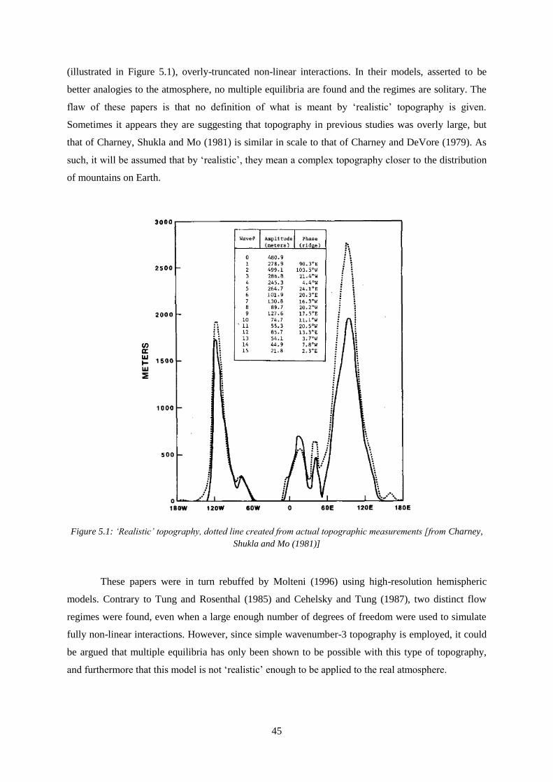
(illustrated in Figure 5.1), overly-truncated non-linear interactions. In their models, asserted to be
better analogies to the atmosphere, no multiple equilibria are found and the regimes are solitary. The
flaw of these papers is that no definition of what is meant by „realistic‟ topography is given.
Sometimes it appears they are suggesting that topography in previous studies was overly large, but
that of Charney, Shukla and Mo (1981) is similar in scale to that of Charney and DeVore (1979). As
such, it will be assumed that by „realistic‟, they mean a complex topography closer to the distribution
of mountains on Earth.
Figure 5.1: ‘Realistic’ topography, dotted line created from actual topographic measurements [from Charney,
Shukla and Mo (1981)]
These papers were in turn rebuffed by Molteni (1996) using high-resolution hemispheric
models. Contrary to Tung and Rosenthal (1985) and Cehelsky and Tung (1987), two distinct flow
regimes were found, even when a large enough number of degrees of freedom were used to simulate
fully non-linear interactions. However, since simple wavenumber-3 topography is employed, it could
be argued that multiple equilibria has only been shown to be possible with this type of topography,
and furthermore that this model is not „realistic‟ enough to be applied to the real atmosphere.

46
Similarly, Risch (1999) claimed to find laboratory evidence for multiple equilibria in a
thermally-forced annulus for both with and without topography. The topography used was a simple
wavenumber-2 shape, suggesting that (like in Molteni (1996), above) low-order models that found
multiple equilibria with similar topography were not seeing a false positive due to their „overly-
truncated non-linear interactions‟, as alleged by Tung and Rosenthal (1985) and Cehelsky and Tung
(1987). By extension, Risch (1999) notes that this implies that multiple equilibria should also be
possible in the baroclinic atmosphere. The need for „realistic‟ topography is still an issue, however.
Supporting the other side of the argument, Tian et al (2001)9 compared similar numerical and
laboratory annulus studies, finding stable multiple equilibria to be prevalent in the former, but not to
exist at all in the latter. The physical annulus still produced both zonal and blocked regimes, but they
were meta-stable, with irregular, sudden transitions. The lack of multiple equilibria could be due to
the fact that the annulus is barotropic (forced by jets) as well as the topography being a simple
wavenumber-2 type. No transitions were observed in the computational model, possibly due to the
lack of three-dimensional effects (this is to be verified via further numerical simulations).
Recent works, such as Koo and Ghil (2002) and others by the same authors, claim that
multiple equilibria can be observed in their models with realistic topography and fully-realised non-
linearity. However, the study is, by the authors‟ own admission, carried out on a low-order model.
In an annulus, though the atmospheric model is simplistic, the non-linear interactions will not
be truncated, giving a perfectly „realistic‟ flow. Unfortunately, creating „realistic‟ topography is more
difficult than in a numerical model, especially if fine features are required. If this problem can be
overcome, the topography of Charney, Shukla and Mo (1981) can be recreated – with this „realistic‟
topography and the fully non-linear interactions of a physical annulus, a definitive investigation into
the existence of multiple equilibria could be launched, putting to the test every condition of Tung and
Rosenthal (1985) and Cehelsky and Tung (1987) simultaneously.
By going one step further, this could become a new experiment in its own right: carrying out
a simple study with basic wavenumber-2 type topography, and then replacing the bottom surface with
increasingly more complex mountain distributions (different elevations, asymmetrical locations, lesser
peaks etc) until no further difference between results can be detected. This would give a reasonable
definition for a „realistic‟ topography and could then be applied to the investigation into multiple
equilibria as a future study. Naturally, this experiment would be easier for a computational model, to
save having to build many different iterations of the topography, as well as removing the time-
consuming task of emptying and refilling the annulus every time each new topography was used.
9 This paper appears to change the meaning of „meta-stable‟ from „can transition from one regime to another‟, to
„will transition between the regimes‟. Hence, the „meta-stable‟ states in Charney and DeVore (1979), that allow
multiple equilibria, are re-classified as „stable‟ by Tian et al (2001).

47
However, the benefits of finding a compromise between realism and manufacturing difficulty could
lead to the creation of a standard „Earth‟ topography for use in many future annuli studies.
In a similar vein to the search for „realistic‟ topography, an unresolved question exists in what
type of topography should be employed. Practically all differentially heated annuli use sinusoidal
topography. However, this can range from a simple wavenumber-2 type, as seen in Bernardet et al
(1990), through a simple wavenumber-3 type shown in Risch (1999), to a non-axisymmetric
wavenumber-5 type, found in Jonas (1981). A further option is for radial variation: Li, Kung and
Pfeffer (1986) carried out experiments with radially uniform topography, but Leach (1981) included a
slope so that his topography was greater near to the outer wall.
In numerical studies as well, a sinusoidal bottom surface as shown in Charney and DeVore
(1979) is the most common. Again there is no standard, and both wavenumber-2, as in Li, Kung and
Pfeffer (1986), and wavenumber-3, as in Molteni (1996), types are widespread, due to similarities to
the topographies of Earth and Mars. Less regular shapes are also possible, such as Yang, Reinhold and
Källén‟s (1997) single isolated mountain and Charney, Shukla and Mo‟s (1981) uneven topographic
distribution based on actual measurements of Earth‟s mountain ranges.
Which choices are made are up to each individual author‟s judgement of what arrangement of
equipment creates a good simulation of the atmospheric circulation without over-simplification or
over-complication. However, it stands to reason that some types of topography will produce better
simulations of the Earth (or whichever planet is the focus of interest) than others. This leads back to
the concept of the search for a standard „Earth‟ topography – experiments could determine whether
radially uniform or radially sloped topography (for example) was a better compromise between
realism and manufacturing difficulty, and thus declare that to be the superior representation.
A number of unresolved questions about the effects of topography on the atmosphere could
be posed on the more unusual findings of Risch (1999). A strange occurrence was found whereby, for
low Taylor number and medium Rossby number flows, a wave-3 stationary wave was found to grow a
fourth „wave-lobe‟ (Figure 5.2) at low levels, but not at high levels. This could possibly be showing
an example of blocking, and could be examined via further study of that region of parameter space. A
second question concerns the understanding of stratospheric sudden warmings, a mysterious
phenomena of the atmosphere, although they are known to be caused by seasonal variations.
Changing the temperature difference over longer time-scales could mimic these seasonal variations,
thus leading to a study of stratospheric sudden warmings. Finally, a lesser question is the relative

48
scales of the effects of thermal and topographic forcing on the rise of stationary waves. This could be
investigated by using insulating material (or similar) to only allow a temperature difference on the
upper half of the annulus, hence comparing the thermally-forced upper half to the topographically-
forced lower half.
Figure 5.2: Wavenumber-3 structure with rogue ‘wave-lobe’ at low level, [from Risch (1999)]
Unfortunately, without a re-design of the annulus, the addition of insulating material for the
forcing comparison experiment would cause interference with the flow, unless the material was very
thin, at which point the insulating properties may not be strong enough to separate the thermal
forcing. A fair amount of work would be needed to rectify this. The investigation into seasonal
variations seems more feasible, with it also appearing to be a more interesting area of research and the
most relevant to the atmosphere. Additionally, improving a laboratory study so that it more closely
resembles the long-term atmospheric circulation would allow for study of oscillations with much
longer periods than currently possible in a physical annulus. The rogue „wave-lobe‟ discovered bears
some similarity to the findings of the bifurcation study, so spatial period-doubling may be a cause.
Future experiments with the same apparatus should be able to investigate this possibility further,
particularly when images can be taken from all levels.

49
A more mathematical unresolved question, based on the comments of Benzi et al (1986), is
that there is difficulty in writing a single equation for the zonal flow over topography. This is due to a
poor assumption for the calculation of form drag, a complicated feedback between topography waves
and zonal wind, and the fact that non-geostrophic effects (such as boundary layer separation and
topography steepness) are ignored.
Whilst form drag is a very interesting aspect of topography, with numerous parallels to other
topics in fluid dynamics including nautical and aerospace engineering, a laboratory study such as an
annulus cannot give an equation for zonal wind directly, like a numerical model could. However, a
physical study could shed some light on which non-geostrophic parameters affect zonal wind, and by
how much. In addition, if time permits, the planned numerical study for the subsequent years of this
thesis (see Chapter 6) may be adapted to attempt to answer this question.
A recent open question concerns the origin of Low-Frequency Variability (alternatively Low-
Frequency Vacillation, shortened to LFV). LFV is defined by Koo and Ghil (2002) as the variability
of the atmosphere with a time scale longer than major weather phenomena (5-6 days) but shorter than
seasonal variability (about 100 days). Naturally, this means that the variability is extremely important
for weather predictions and forecasting. The authors state that it is dominated by atmospheric zonal
flow vacillation, and that it is often caused by non-linear interactions and transitions between multiple
equilibria regimes, but the precise mechanism for its formation is still unresolved.
In a related subject to the above, Ghil and Robertson (2002) divided the topic of LFV into
planetary flow regimes (“particles”) and intraseasonal oscillations (“waves”). They state that it is
unknown whether the former are slow phases of the latter, or the latter are instabilities of the former.
The authors note that both are fundamentally important, and knowing their relationship will greatly
increase predictability of the atmosphere.
Kondrashov, Ide and Ghil (2004) revisited this latter issue, seemingly leaning towards the
idea that the slow phases of the oscillations denote the locations of the unstable equilibria, but decide
that an in-depth analysis is “beyond the purpose of the present paper”.
The origins and internal relationships of LFV would be a difficult question to answer in an
annulus, though the topographically forced oscillatory instability discussed by Ghil and associates
could be looked at in further detail. The transitions between regimes in the annulus and their
counterparts in the atmosphere could also be studied, perhaps as part of a larger study into multiple
equilibria.

50
Despite plentiful research in the area, a question remains of the precise effects of adding a
small amount of topographic variation, as opposed to a flow over a flat surface. One of the most
surprising and unusual effects of topography known from numerical models, for example Charney
and DeVore (1979), is that low topography can actually act to stabilise a given flow, requiring a
greater thermal forcing (or rotation rate, depending on what parameter is held constant) to produce
instabilities. Cehelsky and Tung (1987) provide Figure 5.3 to illustrate this concept.
Figure 5.3: Representation of flow stability (represented by the y-axis, a higher value implying greater stability)
against topographic height showing initial stabilisation and peak at low topography [from Cehelsky and Tung
(1987)]
Jonas (1981) was the first to attempt to apply this effect to a physical annulus, using an
increase in rotation rate rather than an increase in thermal forcing. Using a simple analysis, the author
predicted the effects of the addition of topography, including an increase in rotation needed before the
transition to baroclinic waves is reached, an increase in wavenumber of these waves and a decrease in
length of the baroclinic waves. The predictions were backed up by the observations taken, but only
qualitatively. The author noted that the analysis is “grossly inaccurate” when applied to the real
annulus, not least because boundary-layer separation (which would imply zero vertical velocity at the
top and bottom) cannot be observed. He also mentioned that: “calculations of the spatial growth rates
of perturbations in flows of spatially varying static stability would provide useful information on this
mechanism”.
Both blocking and zonal flow regimes were investigated in Tian et al (2000), with focus on
their spatial and temporal characteristics. A numerical study is compared with a laboratory annulus,
noting the spatial similarity of both experiments, including the shape and location of the flow vortices
and the configuration and magnitude of the jet. No growth rate is given, however, and the annulus is
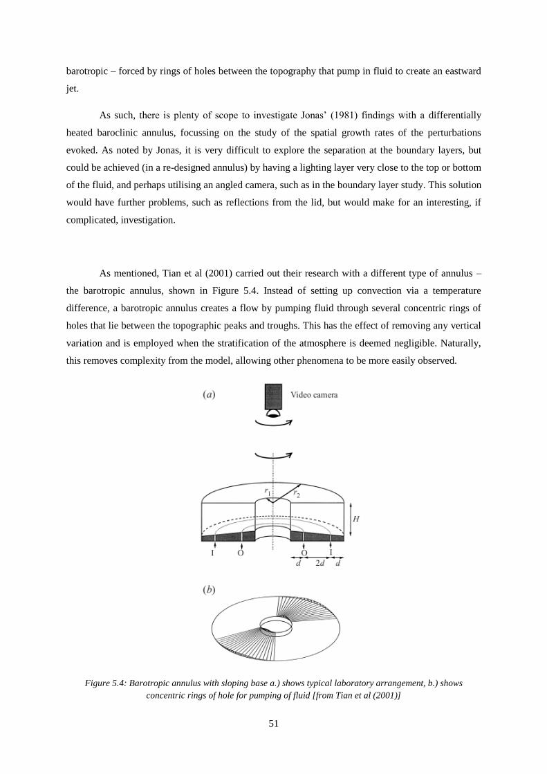
51
barotropic – forced by rings of holes between the topography that pump in fluid to create an eastward
jet.
As such, there is plenty of scope to investigate Jonas‟ (1981) findings with a differentially
heated baroclinic annulus, focussing on the study of the spatial growth rates of the perturbations
evoked. As noted by Jonas, it is very difficult to explore the separation at the boundary layers, but
could be achieved (in a re-designed annulus) by having a lighting layer very close to the top or bottom
of the fluid, and perhaps utilising an angled camera, such as in the boundary layer study. This solution
would have further problems, such as reflections from the lid, but would make for an interesting, if
complicated, investigation.
As mentioned, Tian et al (2001) carried out their research with a different type of annulus –
the barotropic annulus, shown in Figure 5.4. Instead of setting up convection via a temperature
difference, a barotropic annulus creates a flow by pumping fluid through several concentric rings of
holes that lie between the topographic peaks and troughs. This has the effect of removing any vertical
variation and is employed when the stratification of the atmosphere is deemed negligible. Naturally,
this removes complexity from the model, allowing other phenomena to be more easily observed.
Figure 5.4: Barotropic annulus with sloping base a.) shows typical laboratory arrangement, b.) shows
concentric rings of hole for pumping of fluid [from Tian et al (2001)]

52
The numerical equivalent to the barotropic annulus is the one-layer model, compared to the
two-layer baroclinic model. One-layer models reduce the simulation to barotropic to decrease
computational expense when vertical structure is not needed. This type of model is almost as common
as the two-layer type, with examples occurring in Charney and DeVore (1979) and Benzi et al (1986).
One-layer models also appear to be the standard for studies of Martian topography, with both
Keppenne (1992) and Keppenne and Ingersoll (1995) using barotropic shallow-water experiments in
their papers.
This raises the obvious question – how far do barotropic and baroclinic models with
topography differ? Furthermore, how does adding baroclinic structure affect the results of barotropic
models? This could be investigated by replicating the results of Tian et al (2001) in a baroclinic
annulus, or by using a one-layer numerical model under the same parameters as an annulus
experiment.
Finally, it should be noted that, since the focus of this project is the interactions of topography
with the atmospheric circulation, the majority of the literature examined is based on the dynamics of
the atmosphere. The oceans experience topography as well and there is plenty of scope for
comparison between the two. One of the major differences is the forcing of the flow: atmospheric
studies, like all those mentioned above, are thermally-driven; oceanic studies, like Völker (1999) who
simulated the Antarctic Circumpolar Circulation, are wind-driven. Without that distinction, the latter‟s
study is difficult to distinguish from a standard atmospheric study, employing a baroclinic quasi-
geostrophic channel model.
This being the case, it would form an interesting study to compare the oceans and the
atmosphere within the annulus. This could be achieved by creating simple ocean-like topography, for
example tall „blocks‟ that could be dropped into the annulus, trapping the bottom layer, like the ocean
basin experiments of Wordsworth (2008), except in that case the vertical walls used blocked the entire
depth of the fluid. Alternatively, the ocean forcing could be simulated by replacing the heating and
cooling systems with an array of fans to drive the flow. The current annulus in use would probably not
make the best choice for either of these options (especially not the latter) due to its large size, but a
smaller annulus could be converted relatively quickly and easily.
53
5.2 Proposed Topographic Study
In conclusion, the existence of multiple equilibria is still the biggest unresolved question in
topography, even if it is not as controversial a topic as it once was in the period after Tung and
Rosenthal (1985) and Cehelsky and Tung (1987) published their papers. However, the most
immediate aspect of this issue is how best to create a topography for an annulus that can be defined as
„realistic‟. For the sake of clarity, instead of the term „realistic‟, from now on the topography
investigated will be referred to as „less-idealised‟. This issue was brought up in Li, Kung and Pfeffer
(1986). In that paper, a simple wavenumber-2 type topography was employed, but it is noted that the
real topographic distribution of Earth (and other planets) is much more complicated. The authors
expressed a wish to repeat their experiments with a better model of this distribution, suggesting a
superposition of the Fourier components of wavenumber-1 and wavenumber-2. Taking the idea of an
improved topographic distribution was brought to its logical conclusion in Boyer and Chen (1987),
where one mountain range in particular, in this case the Rocky Mountains, was modelled in great
detail for a laboratory experiment. Conversely, however, this paper was criticised for bringing too
much complexity to such a simple simulation of the atmosphere. James (1988), for example, noted
that having such a detailed topography was of dubious worth when the walls of the annulus will
produce reflection patterns that simply do not exist in the flow over the Rocky Mountains. From this,
the lesson learnt is that less-idealised topography should not be a hyper-realistic reproduction of a
planet‟s surface. Instead, a smaller change to basic sine wave topography is needed, to reflect the
limitations of the physical annulus model. As such, the original idea of Li, Kung and Pfeffer (1986)
can be revisited: using a superposition of wavenumbers to create a less-idealised distribution.
Hence, the subject of this thesis will be an investigation into the various superpositions of the
first three wavenumbers. For example, the Fourier decomposition of the Southern Hemisphere of
Mars, from Hollingsworth and Barnes (1996), suggests that its topography is formed from both a
wavenumber-1 and a wavenumber-3. This is illustrated in Figure 5.5. The proposed study is therefore
to carry out experiments with both of these types of topography separately (or just the wavenumber-3
type, if time does not permit both) at known points in parameter space, and then investigate a
topography formed from their superposition under the same conditions. Not only will this highlight
the effects of combining wavenumbers but it should furthermore give a reasonably accurate model for
the Southern Hemisphere of Mars. In addition, the results of experiments under less-idealised
topography may also go some way to answering the open questions of the previous section,
confirming or denying the existence of multiple equilibria and determining the mechanism of
formation for LFV, for example.
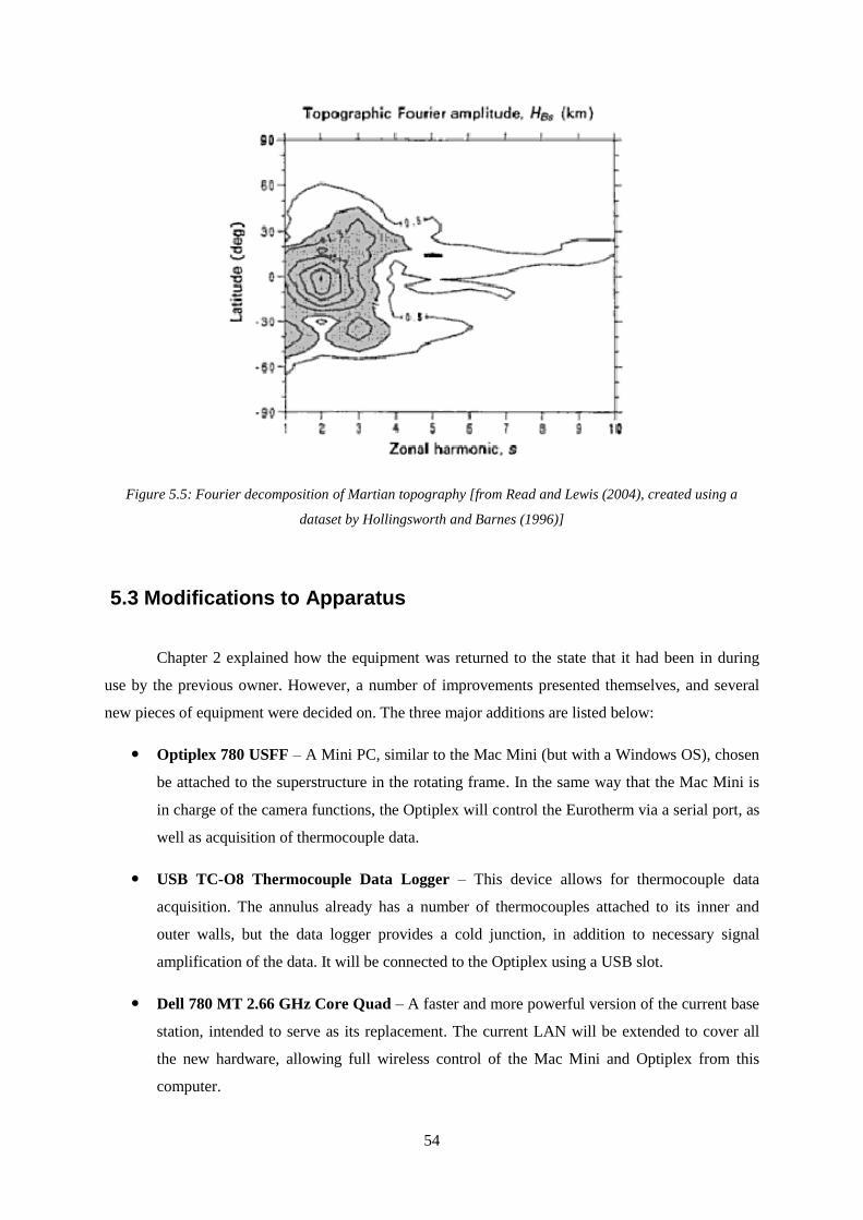
54
Figure 5.5: Fourier decomposition of Martian topography [from Read and Lewis (2004), created using a
dataset by Hollingsworth and Barnes (1996)]
5.3 Modifications to Apparatus
Chapter 2 explained how the equipment was returned to the state that it had been in during
use by the previous owner. However, a number of improvements presented themselves, and several
new pieces of equipment were decided on. The three major additions are listed below:
Optiplex 780 USFF – A Mini PC, similar to the Mac Mini (but with a Windows OS), chosen
be attached to the superstructure in the rotating frame. In the same way that the Mac Mini is
in charge of the camera functions, the Optiplex will control the Eurotherm via a serial port, as
well as acquisition of thermocouple data.
USB TC-O8 Thermocouple Data Logger – This device allows for thermocouple data
acquisition. The annulus already has a number of thermocouples attached to its inner and
outer walls, but the data logger provides a cold junction, in addition to necessary signal
amplification of the data. It will be connected to the Optiplex using a USB slot.
Dell 780 MT 2.66 GHz Core Quad – A faster and more powerful version of the current base
station, intended to serve as its replacement. The current LAN will be extended to cover all
the new hardware, allowing full wireless control of the Mac Mini and Optiplex from this
computer.

55
With these new pieces of equipment, the camera will cease to be the sole source of data and
the fluid temperature field can also be observed and studied. Despite the thermocouples being only
attached to the inner and walls, and not protruding into the flow itself (which would cause
unavoidable interference, as found by Leach (1981) and Hignett at el (1985), for example), the
information gathered should provide greater detail of the baroclinic structure of the fluid and act as a
comparison to the camera‟s flow velocity data for the study of topography. Such an arrangement was
employed by Pfeffer, Kung and Li (1988) for their similar work to good effect. This temperature data
will also be invaluable in the investigation of thermal boundary layers, if the study of inertia-gravity
waves is resumed. An existing LabVIEW control system will be also adapted for future experiments,
allowing manipulation of the rotation rates and temperature differences from a single program on the
new base station (as well as ensuring that they are continuous).
A secondary purpose for the experiments of the first year was to ascertain the condition and
working order of the apparatus. Whilst the various leaks of the heating and cooling systems had no
practical impact on the investigation, and therefore could safely be ignored, the lighting array was
found to be far more problematic. At some point prior to the beginning of this thesis the metal of the
array had seemingly deformed, causing the lights to no longer exactly match up with their respective
slits in the annulus. As such, the illumination was below optimal, especially at lower levels. Whilst
this issue could be fixed, it seems prudent to replace the array of lamps with one of Ultra-Bright
LEDs. Not only would this fix the illumination problem, but the light would be more focussed and
less susceptible to picking up particles outside of its level. In addition, the three electric fans could be
removed, reducing weight and clutter on the rotating frame.
56
Chapter 6
Further Work and Timeline
This chapter will summarise all the tasks planned for the next two years of this thesis. Firstly,
the experiments devised in the last section of Chapter 4 to improve the bifurcation and inertia-gravity
wave studies will be condensed. After that, the proposed topographic study of Chapter 5 will be
broken into individual tasks. In the next section, a planned numerical study to complement the
laboratory work will be discussed and its importance explained. Finally, a timeline is provided to
illustrate when all of these tasks are planned to take place in the course of the thesis.
6.1 Further Work – First Year Studies
There are essentially four extensions to the studies conducted in this report. The first
extension, for the bifurcation study, is to either replace the current annulus with a smaller version, as
shown in Figure 2.7, or to construct a thermocouple array that can take temperature data across the
entire flow profile. Whichever solution is chosen, the experiments will be performed in the same way
as before – this time closer to the location of the bifurcation sequence. The second extension, also for
the bifurcation study, is to continue to use the same annulus to examine the same area in parameter
space as the Low Taylor Number experiments, with the aim of investigating further spatial period-
doubling events. The third extension, for the inertia-gravity wave study, is to build an improved
arrangement of equipment, with superior lighting sources and injection methods. The fourth
extension, also for the inertia-gravity wave study, is to carry out more experiments over a greater
number of points in parameter space, optimally with continuous control over rotation rates and
temperature differences.
The two preliminary studies would then be able to develop into six new investigations:
A repeat of the bifurcation study with a standard annulus or an extensive thermocouple array.
A development of the bifurcation study with the goal of finding spatial period-doubling.
An investigation into the limits of parameter space for where inertia-gravity waves occur.
A comparison of instability rolls in water and water-glycerol mixture.
A search for multiple instability rolls under any conditions.
An examination of the effects of adding a rigid lid on the thermal boundary layer.
57
6.2 Further Work - Topography
As explained in Chapter 5, the major focus of the subsequent years of this thesis will be based
upon improving the laboratory representation of topography by making it less idealised, the impact of
this improvement on atmospheric circulation and whether the result creates a more appropriate
topography for use in other laboratory and numerical experiments, as well as weather prediction
models. Topography will be designed as a superposition of wavenumbers, based on Hollingsworth
and Barnes‟ (1996) description of the Southern Hemisphere of Mars, to observe the effects of this
superposition against simple wavenumber topography.
The opening task of the topographic study is to re-design the apparatus. Adding the Dell 780
MT 2.66 GHz Core Quad, the Optiplex 780 USFF and the USB TC-O8 Thermocouple Data Logger,
as well as setting up a LabVIEW control system, will allow thermocouple data to be received and
continuous remote manipulation over the rotation rates and temperature differences from the base
station to be achieved. In addition, the lighting array requires replacing with one comprising of Ultra-
Bright LEDs. At the same time, the three different topographic bases – wavenumber-1, wavenumber-
3 and the superposition of the two – will be designed and sent off to be built. If the construction of the
topography takes longer than expected, the wavenumber-1 base will be abandoned, and the
investigation will solely focus on the other two.
The topography will be designed so that the peaks and troughs are large enough to begin to
invalidate quasi-geostrophic theory, as explained in the next section. The topography will also include
a 22° radial slope downwards from the inner wall to the outer wall. The slope simulates the beta effect
of the atmosphere, which is otherwise ignored. This particular gradient was chosen due to the work of
Wordsworth (2008), who created a similarly sloping Perspex lid (also necessary for the beta effect),
carefully designing it so no optical properties were lost.
The experiments will first be carried out with the wavenumber-3 base, noting the differences
to the flat-bottomed bifurcation study and determining locations of parameter space that provide
repeatable, well-defined wave structures. The topography will then be replaced by the wavenumber-1
and the superposition bases, observing the differences to the flow under the same conditions. In this
way, the investigation of superposition topography will begin, allowing for the possibility of further
studies and extensions as progress is made. The objective of these further studies will be to find
solutions to the open questions posed in Chapter 5, such as the growth-rate and time-scale of the
various topographically forced oscillations and perturbations, the existence of multiple equilibria with
less-idealised topography and the mechanism of generation of LFV. The apparatus could even be
adapted further, for example by varying the long-term temperature difference to allow the seasonal
58
variation experiment suggested by Risch (1999), or by the addition of topographic „blocks‟ to permit
comparison to ocean circulation.
6.3 Numerical Study
QUAGMIRE, standing for QUAsi-Geostrophic Model for Investigating Rotating fluids
Experiments, is different to those numerical models most commonly used in the literature (as
mentioned in Chapter 5), as it is not employed to search for new atmospheric phenomena, but instead
to increase the understanding of those already found. As the name suggests, it attempts to achieve this
by having its geometry in the form of a rotating annulus like those used in laboratory. Unlike the
otherwise similar MORALS (Met Office/Oxford Rotating Annulus Laboratory Simulation, see Farnell
and Plumb (1975) for a full description), instead of challenging the full Navier-Strokes Equations and
the many other equations that describe a flow, QUAGMIRE only solves the quasi-geostrophic
potential vorticity equation. Williams, Read and Haine (2010) explained that, due to their simplicity
and thus their ease of modelling, laboratory flows are excellent for studying “fundamental dynamical
phenomena”. However, the authors believed that models that solve the Navier-Strokes Equations are
too computationally expensive to use for a large enough sample of flows. QUAGMIRE is the solution
to this problem, with its greatly reduced computational expense. The model is also multi-layer,
allowing the vertical structure of the atmosphere to be investigated as rigorously or as roughly as
required10
. On the other hand, the use of the quasi-geostrophic approximation means that no
ageostrophic features of the flow can be simulated. The most notable absence is the boundary layers,
which in turn means no Ekman Layers can exist. The remedy for this is to set boundary conditions via
Ekman Pumping, but ageostrophic features will still not be modelled.
The reasoning behind using QUAGMIRE is twofold: firstly, as Hignett et al (1985) noted, an
additional numerical study can greatly improve the accuracy of a laboratory study. The numerical
model QUAGMIRE, already set up to simulate a differentially-heated annulus, will be employed for
the same topographies, allowing comparison between the experimental and computational studies.
The results gathered from these experiments will be contrasted, highlighting and removing as many
errors as possible and hence reducing the risk of nonsense readings from either source.
10
One- and two-layer models have already been discussed and, for example, Kondrashov, Ide and Ghil (2004)
achieved a „realistic‟ global simulation using a three-layer model.

59
Secondly, and most importantly, QUAGMIRE is a quasi-geostrophic model. Comparing its
results to those from the physical annulus will test the limits of quasi-geostrophic theory. The theory
is known to begin to break down at roughly the point where the ratio of the height of the topography
to the height of the annulus becomes greater than or equal to the Rossby Number of the flow. This is
what occurs in the atmosphere, if the height of the annulus is replaced by the height of the tropopause.
As such, the magnitude of the topography designed, as well as the flow parameters used, will be
chosen in such a way that this condition is met. The comparisons between the experiments will
therefore show how well a quasi-geostrophic model copes in an ageostrophic environment and which
ageostrophic aspects of sloped convection, if any, can be imitated. In addition, any flow features
observed in the laboratory study, but not the numerical study, can be assumed to be ageostrophic in
nature.
6.4 Timetable
Figure 6.1 shows an estimated timeline of this project, running from the current time until its
end in the summer of 2012. The length of time allotted to each task is intentionally generous, to take
into account the various potential delays for those assignments (such as long delivery times for parts).
Hopefully, this will also mitigate the effect of any unforeseeable problems encountered (such as
equipment failure or illness). As topography is the main focus of the second and third year of this
thesis, the further studies into bifurcations and inertia-gravity waves will not be explicitly factored
into the planned timeline. The penultimate task, however, is amongst the longest, allowing ample
scope for further studies and experiments to be carried out, if the project does not fall behind
schedule.
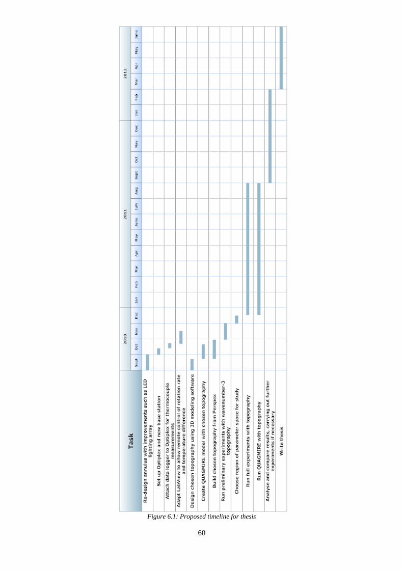
60
Figure 6.1: Proposed timeline for thesis

61
Chapter 7
References
Andrews, D.G., 2000. An Introduction to Atmospheric Physics. Cambridge: Cambridge University
Press.
Benzi, R., Malguzzi, P., Speranza, A. & Sutera, A., 1986. The Statistical Properties of General
Atmospheric Circulation: Observational Evidence and a Minimal Theory of Bimodality. Quarterly
Journal of the Royal Meteorological Society, 112(473), pp.661-674.
Bernardet, P., Butet, A., Déqué, M., Ghil, M. & Pfeffer, R.L, 1990. Low Frequency Oscillations in a
Rotating Annulus with Topography. J. Atmos. Sci., 47(24), pp.3023-3043.
Boyer, D.L. & Chen. R., 1987. Laboratory Simulations of Mechanical Effects of Mountains on the
General Circulation of the Northern Hemisphere: Uniform Shear Background Flow. J. Atmos. Sci.,
44(23), pp.3552-3575.
Cehelsky, P. & Tung, K.K., 1987. Theories of Multiple Equilibria and Weather Regimes – A Critical
Reexamination. Part II: Baroclinic Two-Layer Models. J. Atmos. Sci., 44(21), pp.3282-3303.
Charney, J.G. & DeVore, J.G., 1979. Multiple Flow Equilibria in the Atmosphere and Blocking. J.
Atmos. Sci., 36(7), pp.1205-1216.
Charney, J.G. & Straus, D.M., 1980. Form-Drag Instability, Multiple Equilibria and Propagating
Planetary Waves in Baroclinic, Orographically Forced, Planetary Wave Systems. J. Atmos. Sci.,
37(6), pp.1157-1176.
Charney, J.G., Shukla, J. & Mo, K.C., 1981. Comparison of a Barotropic Blocking Theory with
Observation. J. Atmos. Sci., 38(4), pp.762-779.
Chomaz, J.M., Rabaud, M., Basdevant, C. & Couder, Y., 1988. Experimental and Numerical
Investigation of a Forced Circular Shear Layer. J. Fluid Mech., 187, pp.115-140.
Farnell, L. & Plumb, R.A., 1975. Numerical Integration of Flow in a Rotating Annulus I:
Axisymmetric Model. Occasional Note Met O, 21 75/3. [Unpublished Technical Report]
Fein, J.S. & Pfeffer, R.L., 1976. An Experimental Study of the Effects of the Prandtl Number on
Thermal Convection in a Rotating, Differentially Heated Cylindrical Annulus of Fluid. J. Fluid
Mech., 75(1), pp.81-112.
62
Ghil, M. & Robertson, A.W., 2002. “Waves” vs. “Particles” in the Atmosphere‟s Phase Space: A
Pathway to Long-Range Forecasting? Proceedings of the National Academy of Sciences of the United
States of America, 99(1), pp.2493-2500.
Gollub, J.P. & Benson, S.V., 1980. Many Routes to Turbulent Convection. J. Fluid Mech., 100(3),
pp.449-470.
Hart, J.E., 1985. A Laboratory Study of Baroclinic Chaos on the f-Plane. Tellus A, 37A(3), pp.286-
296.
Held, I.M., 1983. Stationary and Quasi-Stationary Eddies in the Extratropical Troposphere: Theory. In
Hoskins, B.J. & Pearce, R.P., ed., Large-Scale Dynamical Processes in the Atmosphere. London:
Academic Press Inc. (London) Ltd. Ch. 6.
Hide, R., 1953. Some Experiments on Thermal Convection in a Rotating Liquid. Quarterly Journal of
the Royal Meteorological Society, 79(339), pp.161. [Correspondence]
Hide, R., 1958. An Experimental Study of Thermal Convection in a Rotating Liquid. Philosophical
Transactions of the Royal Society of London. Series A, Mathematical and Physical Sciences,
250(983), pp.441-478.
Hide, R., Lewis, S.R. & Read, P.L., 1994. Sloping Convection: A Paradigm for Large-Scale Waves
and Eddies in Planetary Atmospheres? Chaos, 4(2), pp.135-162.
Hide, R. & Mason, P.J., 1975. Sloping Convection in a Rotating Fluid. Advances in Physics, 24(1),
pp.47-100.
Hignett, P., White, A.A., Carter, R.D., Jackson, W.D.N. & Small, R.M., 1985. A Comparison of
Laboratory Measurements and Numerical Simulations of Baroclinic Wave Flows in a Rotating
Cylindrical Annulus. Quarterly Journal of the Royal Meteorological Society, 111(463), pp.131-154.
Hollingsworth, J.L. & Barnes, J.R., 1996. Forced Stationary Planetary Waves in Mars‟s Winter
Atmosphere. J. Atmos. Sci., 53(3), pp.428-448.
Houghton, J., 2002. The Physics of Atmospheres. 3rd
ed. Cambridge: Cambridge University Press.
Jacoby, T.N.L., Read, P.L., Williams, P.D. & Young, R.M.B., 2010. Generation of Inertia-Gravity
Waves in the Rotating Thermal Annulus by a Localised Boundary Layer Instability. [Unpublished]
James, I.N., 1988. Meteorology of a Flat Earth. Nature, 333, pp.118.
Jonas, P.R., 1981. Laboratory Observations of the Effects of Topography on Baroclinic Instability.
Quarterly Journal of the Royal Meteorological Society, 107(454), pp.775-792.

63
Keppenne, C.L., 1992. Orographically Forced Oscillations in a Dynamical Model of the Martian
Atmosphere. Icarus, 100(2), pp.598-607.
Keppenne, C.L. & Ingersoll, A.P., 1995. High-Frequency Orographically Forced Variability in a
Single-Layer Model of the Martian Atmosphere. J. Atmos. Sci., 52(11), pp.1949-1958.
Kondrashov, D., Ide, K. & Ghil, M., 2004. Weather Regimes and Preferred Transition Paths in a
Three-Layer Quasigeostrophic Model. J. Atmos. Sci., 61(5), pp.568-587.
Knox, J.A., McCann, D.W. & Williams, P.D., 2008. Application of the Lighthill-Ford Theory of
Spontaneous Imbalance to Clear-Air Turbulence Forecasting. J. Atmos. Sci., 65(10), pp.3292-3304.
Koo, S. & Ghil, M., 2002. Successive Bifurcations in a Simple Model of Atmospheric Zonal-Flow
Vacillation. Chaos, 12(2), pp.300-309.
Leach, H., 1981. Thermal Convection in a Rotating Fluid: Effects due to Bottom Topography. J. Fluid
Mech., 109, pp.75-87.
Li, Q.G., Kung, R. & Pfeffer, R.L., 1986. An Experimental Study of Baroclinic Flows with and
without Two-Wave Bottom Topography. J. Atmos. Sci., 43(22), pp.2585-2599.
Molteni, F., 1996. On the Dynamics of Planetary Flow Regimes, Part II: Results from a Hierarchy of
Orographically Forced Models. J. Atmos. Sci., 53(14), pp.1972-1992.
Pfeffer, R.L., Kung, R. & Li, Q.G., 1988. Some Effects of Rotation Rate on Planetary-Scale Wave
Flows. Theoretical and Applied Climatology, 55(1-4), pp.199-210.
Rabaud, M. & Couder, Y., 1983. A Shear-Flow Instability in a Circular Geometry. J. Fluid Mech.,
136, pp.291-319.
Randriamampianina, A., private communication. [Conversation – 30/07/2010]
Randriamampianina, A., Früh, W.G., Read, P.L. & Maubert, P., 2006. Direct Numerical Simulations
of Bifurcations in an Air-Filled Rotating Baroclinic Annulus. J. Fluid Mech., 561, pp.359-389.
Read, P.L. & Lewis, S.R., 2004. The Martian Atmosphere Revisited: Atmosphere and Environment of
a Desert Planet. Chichester: Praxis Publishing Ltd.
Reinhold, B.B. & Pierrehumbert, R.T., 1982. Dynamics of Weather Regimes: Quasi-Stationary
Waves and Blocking. Mon. Wea. Rev., 110(9), pp.1105-1145.
Risch, S.H., 1999. Large-Scale Wave Interactions in Baroclinic Flow with Topography. DPhil.
University of Oxford.
64
Tian, Y., Weeks, E.R., Ide, K., Urbach, J.S., Baroud, C.N., Ghil, M. & Swinney, H.L., 2001.
Experimental and Numerical Studies of an Eastward Jet over Topography. J. Fluid Mech., 438,
pp.129-157.
Tung, K.K. & Rosenthal, A.J., 1985. Theories of Multiple Equilibria and Weather Regimes – A
Critical Reexamination. Part I: Barotropic Models. J. Atmos. Sci., 42(24), pp.2804-2819.
Vettin, F., 1857. Ueber den aufsteigenden luftstrom, die entstehung des hagels und der wirbel-
stuerme. Annalen der Physik, 178(10), pp.246-255.
Völker, C., 1999. Momentum Balance in Zonal Flows and Resonance of Baroclinic Rossby Waves. J.
Phys. Oceanogr., 29(8), pp.1666-1681.
Wallace, J.M., 1983. The Climatological Mean Stationary Waves: Observational Evidence. In
Hoskins, B.J. & Pearce, R.P., ed., Large-Scale Dynamical Processes in the Atmosphere. London:
Academic Press Inc. (London) Ltd. Ch. 2.
Williams, G.P., 1967. Thermal Convection in a Rotating Fluid Annulus: Part 2. Classes of
Axisymmetric Flow. J. Atmos. Sci., 24(2), pp.162-174.
Williams, P.D., Read, P.L. & Haine, T.W.N., 2003. Spontaneous Generation and Impact of Inertia-
Gravity Waves in a Stratified, Two-Layer Shear Flow. Geophys. Res. Lett., 30(24), pp.2255-2258.
Williams, P.D., Read, P.L. & Haine, T.W.N., 2010. Testing the Limits of Quasi-Geostrophic Theory:
Application to Observed Laboratory Flows Outside of the Quasi-Geostrophic Regime. J. Fluid Mech.,
649, pp.187-203.
White, F.M., 2008. Fluid Mechanics. 6th ed. New York: McGraw-Hill.
Wordsworth, R.D., 2008. Theoretical and Experimental Investigations of Turbulent Jet Formation in
Planetary Fluid Dynamics. DPhil. University of Oxford.
Yang, S., Reinhold, B. & Källén, E., 1997. Multiple Weather Regimes and Baroclinically Forced
Spherical Resonance. J. Atmos. Sci., 54(11), pp.1397-1409.
Young, R.M.B. & Read, P.L., 2008. Flow transitions resembling bifurcations of the logistic map in
simulations of the baroclinic rotating annulus. Physica D, 237(18), pp.2251-2262.