Slopes of Compact Hecke Operators

Daniel Jacobs

A thesis submitted for the Degree of

Doctor of Philosophy of the University of London

and for the Diploma of Imperial College.

Department of Mathematics

Imperial College of Science, Technology and Medicine

London

January 2003

Prologue

Abstract

In this thesis we present the definitions of the space of automorphic forms over a definite

quaternion algebra. These spaces are infinite dimensional unlike spaces of classical modular

forms which are all known to be finite.

For a general prime number, p, we define a Hecke Operator on this space of automorphic

forms. These operators correspond, via the Jacquet-Langlands correspondence, to the usual

classical Hecke Operators. The point is that spaces of classical modular forms embed into

our space of automorphic forms and study of the Hecke operators on this infinite space gives

us information about the Hecke operators on the classical spaces.

We shall investigate the slopes of a particular operator, U3. The slopes of an operator are

the gradients of the line segments that comprise the Newton polygon of the characteristic

power series of that operator. We prove that, for all κ in a certain disc in weight space, the

slopes of U3 are in arithmetic progression, starting with

12,32,52,72,92,112

, . . . .

Acknowledgements

First and foremost I would like to thank my PhD advisor Kevin Buzzard, for his unfailing

support and wealth of ideas, as well as his unfailing patience, and for taking me on as his

student.

I would like to thank Lloyd Kilford and Ed Nevens, as well as the other Number Theo-

rists, other staff and students of the Mathematics Department of Imperial College for their

help, support and understanding. In particular I would like to thank Lloyd Kilford for his

assistance with programming in MAGMA.

I would like to thank the EPSRC who provided the finance for my studies, the staff

at Imperial College who made studying there an enjoyable experience, the staff at the

Institut Henri Poincare, Paris, where I studied for five months and had access to all facilities

2

3

especially computing ones, and in particular Madame Annie Touchant who helped to ensure

my stay in Paris was enjoyable.

I would like the thank the CRF of the University of London for providing a grant to Kevin

Buzzard for the purchase of the dual-processor computer crackpipe on which many of my

calculations and experiments ran for many hundreds of hours in order to obtain conjectures

about the slopes of Hecke operators.

Lastly I would like to thank my family and friends who provided much support and

healthy distractions from the work.

Contents

Prologue 2

Abstract . . . . . . . . . . . . . . . . . . . . . . . . . . . . . . . . . . . . . . . . . . 2

Acknowledgements . . . . . . . . . . . . . . . . . . . . . . . . . . . . . . . . . . . . 2

Introduction and Brief History 5

1 Definitions and Preliminary Material 6

1.1 Infinite Matrices . . . . . . . . . . . . . . . . . . . . . . . . . . . . . . . . . . 6

1.2 Compact operators . . . . . . . . . . . . . . . . . . . . . . . . . . . . . . . . . 8

1.3 Newton Polygons . . . . . . . . . . . . . . . . . . . . . . . . . . . . . . . . . . 12

1.4 Preliminaries . . . . . . . . . . . . . . . . . . . . . . . . . . . . . . . . . . . . 13

1.5 Automorphic forms . . . . . . . . . . . . . . . . . . . . . . . . . . . . . . . . . 18

1.6 Hecke operators . . . . . . . . . . . . . . . . . . . . . . . . . . . . . . . . . . . 20

2 U3 22

2.1 U3 Evaluated . . . . . . . . . . . . . . . . . . . . . . . . . . . . . . . . . . . . 22

2.2 Extending the Results . . . . . . . . . . . . . . . . . . . . . . . . . . . . . . . 39

Conclusion 41

A Power series calculations 42

B Program Code Listing 44

B.1 U3 Cosets Decompositions . . . . . . . . . . . . . . . . . . . . . . . . . . . . . 44

B.2 W Cosets Decompositions . . . . . . . . . . . . . . . . . . . . . . . . . . . . . 48

B.3 Calculations for U3 with κ(x) = x3. . . . . . . . . . . . . . . . . . . . . . . . . 49

Bibliography 52

4

Introduction and Brief History

Interest in the explicit computation of slopes was first sparked by the work Coleman [Col97],

Emerton [Eme98], Smithline [Smi94] and Coleman-Stevens-Teitelbaum [CST98]. They were

studying overconvergent modular forms and did not prove much beyond facts about the

smallest slope.

For instance, in [Eme98], Emerton proved that for the annulus 1 > |u| ≥ |64| in weight

space, the minimal slope of a Hecke operator, U2, is some explicit function of κ. On the

other hand, Smithline proved in [Smi94], that the average slope of overconvergent 3-adic

modular forms was 3i+1 −1 for certain integers i and that the Newton Polygon of U3 on the

space of 3-adic overconvergent modular forms lies on or above the parabola

3n(n − 1)

2+ 2n.

He was able to compute the minimal slope in a range of cases: tame level 1 and all weights.

Unfortunately, all of these results were only estimates.

In [Kil02], Kilford proves that the operator U2 has slopes in arithmetic progression for

all weights κ of the form x 7→ xk with k ∈ Z, odd. Of course, by continuity, these results

extend to all k ∈ 1 + 2Z2.

The results in this thesis, are the first ever to prove specific things about all the slopes for

all κ in a disc in weight space. In particular, the results are the first explicit computations

of discs in the eigencurve of arbitrarily large weight. However, they tell us nothing about

classical modular forms directly. To do this, it is necessary to use a p-adic version of the

Jacquet-Langlands correspondence (announced by Chenevier) to translate our results to

results about all the slopes of a classical eigencurve over a disc in weight space.

5

Chapter 1

Definitions and Preliminary

Material

In this chapter, we introduce all the preliminary definitions and notations that we require.

We also review some elementary lemmas and theorems both from number theory and ring

theory, as well as the definition of a compact operator and of Hecke operators.

1.1 Infinite Matrices

Here we introduce the notion of an “infinite matrix”, and various manipulations on these

matrices.

1.1 Definition. Let R be a ring1 and suppose that ai,j is a doubly infinite sequence of

elements of R with 0 ≤ i, j,∈ Z. Then, we may form the infinite array:a0,0 a0,1 a0,2 . . .

a1,0 a1,1 a1,2 . . .

a2,0 a2,1 a2,2 . . ....

......

. . .

which we will refer to as a matrix or infinite matrix. Departing from convention, we start

numbering the rows and columns at 0; this is notationally convenient, as we shall see later.

Addition of two such infinite matrices, (ai,j)0≤i,j∈Z and (bi,j)0≤i,j∈Z is pointwise; viz.

(ci,j) := (ai,j) + (bi,j)

where ci,j = ai,j + bi,j for all 0 ≤ i, j,∈ Z. This is well defined and commutative as for the

case of “finite” matrices.1All rings are commutative with a 1.

6

CHAPTER 1. DEFINITIONS AND PRELIMINARY MATERIAL 7

In general, matrix multiplication of infinite matrices is not well defined as there are prob-

lems with convergence in an arbitrary ring, R. However, it will be necessary to pre-multiply

and post-multiply certain matrices by diagonal matrices which do not cause convergence

problems. To this end, we introduce the following notation.

1.2 Notation. Given a sequence, αn (0 ≤ n ∈ Z) of elements in a ring R, we shall write

diag((αn)0≤n∈Z) or diag(α0, α1, α2, . . .) to denote the infinite matrixα0 0 0 . . .

0 α1 0 . . .

0 0 α2 . . ....

......

. . .

. (1.1.1)

If α is an element of R − {0}, we write D(α) for the infinite matrix diag((αn)0≤n∈Z)2, i.e.

D(α) =

1 0 0 . . .

0 α 0 . . .

0 0 α2 . . ....

......

. . .

. (1.1.2)

Multiplication of a given infinite matrix A = (ai,j) by D(α) on the left (respectively

right) simply has the effect of multiplying each entry in row n ∈ Z≥0 (respectively column

n) by αn. Thus, with multiplication by D(α) we do not have any issues concerning infinite

sums in an arbitrary ring.

Given an infinite matrix A = (ai,j), we consider the following formal power series,

HA(x, y) :=∑

0≤i,j∈Zai,jx

iyj ∈ R[[x, y]].

HA(x, y) is called the generating function of the matrix A. If A is sufficiently “nice”, we

can write HA(x, y) as the (formal) quotient of two bivariate polynomials, viz.:

HA(x, y) =FA(x, y)GA(x, y)

with FA(x, y), GA(x, y) ∈ R[x, y]. Whenever such FA and GA exist, we call HA the rational

function of A.

Conversely, given two polynomials F (x, y), G(x, y) ∈ R[x, y] such that the inverse of

G(x, y) exists in R[[x, y]], we may consider the formal series expansion

F (x, y)G(x, y)

=∑

0≤i,j∈Zbi,jx

iyj ∈ R[[x, y]],

2Here, by α0 we, of course, mean 1.

CHAPTER 1. DEFINITIONS AND PRELIMINARY MATERIAL 8

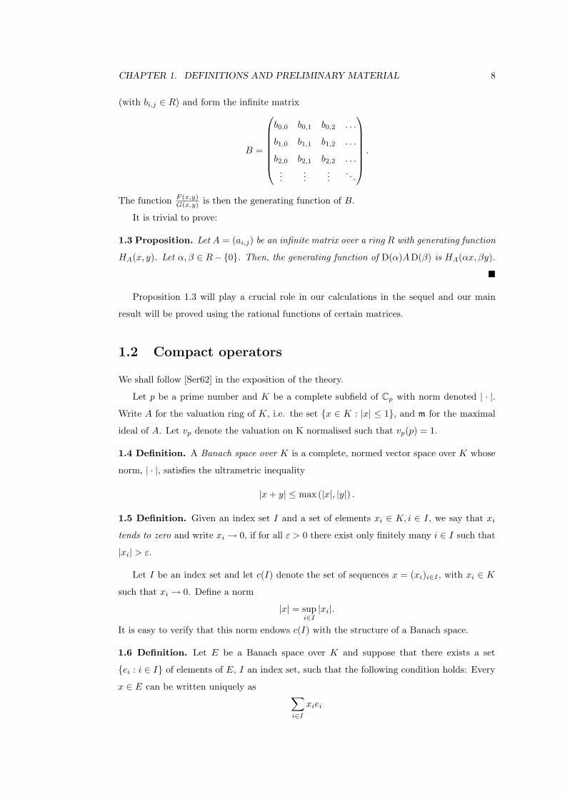
(with bi,j ∈ R) and form the infinite matrix

B =

b0,0 b0,1 b0,2 . . .

b1,0 b1,1 b1,2 . . .

b2,0 b2,1 b2,2 . . ....

......

. . .

.

The function F (x,y)G(x,y) is then the generating function of B.

It is trivial to prove:

1.3 Proposition. Let A = (ai,j) be an infinite matrix over a ring R with generating function

HA(x, y). Let α, β ∈ R−{0}. Then, the generating function of D(α)A D(β) is HA(αx, βy).

�

Proposition 1.3 will play a crucial role in our calculations in the sequel and our main

result will be proved using the rational functions of certain matrices.

1.2 Compact operators

We shall follow [Ser62] in the exposition of the theory.

Let p be a prime number and K be a complete subfield of Cp with norm denoted | · |.

Write A for the valuation ring of K, i.e. the set {x ∈ K : |x| ≤ 1}, and m for the maximal

ideal of A. Let vp denote the valuation on K normalised such that vp(p) = 1.

1.4 Definition. A Banach space over K is a complete, normed vector space over K whose

norm, | · |, satisfies the ultrametric inequality

|x + y| ≤ max (|x|, |y|) .

1.5 Definition. Given an index set I and a set of elements xi ∈ K, i ∈ I, we say that xi

tends to zero and write xi → 0, if for all ε > 0 there exist only finitely many i ∈ I such that

|xi| > ε.

Let I be an index set and let c(I) denote the set of sequences x = (xi)i∈I , with xi ∈ K

such that xi → 0. Define a norm

|x| = supi∈I

|xi|.

It is easy to verify that this norm endows c(I) with the structure of a Banach space.

1.6 Definition. Let E be a Banach space over K and suppose that there exists a set

{ei : i ∈ I} of elements of E, I an index set, such that the following condition holds: Every

x ∈ E can be written uniquely as ∑i∈I

xiei

CHAPTER 1. DEFINITIONS AND PRELIMINARY MATERIAL 9

with xi → 0 and |x| = supi∈I |xi|. Then (ei)i∈I is called an orthonormal basis for E.

Existence of orthonormal bases is straightforward to prove.

We shall restrict ourselves to spaces of the type c(I).

Suppose that E and F are two Banach spaces over K. Write L(E,F ) for the vector

space of continuous, linear maps from E to F . We equip L(E,F ) with the usual norm, viz:

for u ∈ L(E,F )

|u| := supx 6=0

|u(x)||x|

.

This norm gives L(E,F ) the structure of a Banach space.

Write E = c(I) (for an index set I) and assume that (ei)i∈I is an orthonormal basis of

E. If u ∈ L(E,F ), put fi = u(ei). The fi form a bounded family of elements of F . We have

1.7 Proposition ([Ser62], Proposition 3). The map which associates an element u ∈

L(E,F ) to the sequence (u(ei))i∈I is an isomorphism of the Banach space L(E,F ) with the

space of bounded sequences (fi)i∈I of F , equipped with the norm supi∈I |fi|. �

Explicitly, Proposition 1.7 gives us an example of an orthonormal basis for F , and so F

can be identified with c(J) for some index set J . We make this identification. The elements

fi can then be written as (nji)j∈J3 with nji ∈ K, |nji| bounded and nji → 0 for fixed i and

j → ∞. We have,

|u| = supi,j

|nji|

If x = (xi) is an element of c(I), we have u(x) = (yj) with

yj =∑i∈I

njixi.

We shall study the infinite matrix (nji) of u with respect to the orthonormal bases of E and

F ; note that the rows of this matrix are indexed by j ∈ J .

1.8 Definition. Let F(E,F ) denote the subspace of L(E,F ) consisting of the continuous,

linear maps that are of finite rank. We say that u is compact4 if u belongs to the closure of

F(E,F ). Write C(E,F ) for the closure of F(E,F ).

Define rj(u) = supi∈I |nji|. We have

1.9 Proposition ([Ser62], corollary to Proposition 4). The following are equivalent:

1. u is compact.

2. rj(u) tends to zero. �3Note that the reversed subscripts compared with [Ser62] — this is a notational convenience.4In [Ser62], the archaic terminology completely continuous is used.

CHAPTER 1. DEFINITIONS AND PRELIMINARY MATERIAL 10

A useful, special case of this proposition is,

1.10 Corollary. Suppose that the matrix (nji) of u has all its entries in OK . If D(

1p

)(nji)

has all its entries in OK , then u is compact. �

We will often say that a matrix is compact, if it is the matrix of a compact operator with

respect to some basis.

We now introduce the notion of the characteristic power series of an operator.

Let L be a free module over a ring R, and suppose that f is an endomorphism of L

such that f(L) is contained in M — a free sub-module of L of finite type, and a direct

factor of L (e.g. a submodule of L generated by a finite subset of the basis of L). Let

fM : M → M be the restriction of f to M . The polynomial det (1 − tfM ) is well defined,

and it is straightforward to show that it is independent of the choice of M ; write det (1 − tf)

instead. Set

det (1 − tf) = 1 + c1t + . . . + cmtm + . . . .

Suppose that (ei)i∈I is a basis for L and that (nji) is the matrix of f with respect to this

basis.5 We can give the cm explicitly as follows: if S is a finite subset of I, and σ is a

permutation of S write

nS,σ =∏i∈S

nσ(i),i and cS =∑

σ∈Sym(S)

sgn(σ)nS,σ

where Sym(S) is the group of permutations of S and sgn(σ) is the signature of the permu-

tation σ. Thus,

cm = (−1)m∑S⊆I

|S|=m

cS . (1.2.3)

Now we return to compact operators. Assume that u is a compact operator on E and

that |u| ≤ 1. If E0 is the set of elements of E of norm at most 1, we have that u(E0) ⊆ E0.

Assume that a is a non-zero ideal of A contained in m. The operator u now defines, by

passing to the quotient, an endomorphism ua of Ea := E0/aE0; the images of (ei)i∈I in Ea

form a basis (in the algebraic sense) of Ea considered as an A/a-module. If (nji) denotes

the matrix of u with respect to (ei)i∈I and if

rj(u) = supi∈I

|nji|

we have that rj(u) → 0, and there exists a finite subset T (a) of I such that nji ∈ a if

j ∈ I −T (a). It follows that the image of ua is contained in a submodule of Ea of finite type

and that the polynomial det (1 − tua) is well defined. The coefficients of det (1 − tua) lie in

A/a. As a varies, the polynomials form a projective system and their limit is a formal power

5Note that I = J .

CHAPTER 1. DEFINITIONS AND PRELIMINARY MATERIAL 11

series denoted det (1 − tu), whose coefficients tend to zero; this property does not depend

on the product tu. If now, u is any compact endomorphism of E, we can choose a scalar c

such that |cu| ≤ 1 and thus det (1 − tcu) is defined; and hence we may define det (1 − tu) to

be f(

tc

), where f(t) = det (1 − t(cu)).

1.11 Definition. det (1 − tu), as defined above, is called the characteristic power series of

u.

We shall also refer to det (1 − tu) as the characteristic power series of the matrix (nji)

of u.

1.12 Proposition ([Ser62], Proposition 7). Let u : E → E be a compact operator.

1. If the matrix of u with respect to the orthonormal basis (ei)i∈I is (nji) then

det (1 − tu) =∞∑

m=0

cmtm

with cm defined as in (1.2.3).

2. The series det (1 − tu) is an entire function of t, i.e. the radius of convergence is

infinite.

3. If un → u with un ∈ C(E,E) for all n ∈ N, then det (1 − tun) tends to det (1 − tu)

coefficient-wise.

4. If u is of finite rank, then det (1 − tu) coincides with the polynomial defined earlier.

�

1.13 Remark. Parts (3) and (4) of Proposition 1.12 show that det (1 − tu) does not depend

on the norm of E, but only on the topology.

We also have,

1.14 Proposition ([Ser62], Corollary 2 to Proposition 7). Suppose that u ∈ C(E,E)

and v ∈ L(E,E). Then,

det (1 − tu ◦ v) = det (1 − tv ◦ u) .

(Note that this formula makes sense, since u ◦ v, v ◦ u ∈ C(E,E).) �

Lastly,

1.15 Lemma ([Ser62], Lemma 2). Let I = I ′ ∪ I ′′ be a partition of I. Assume that u is

a compact endomorphism of E = c(I) sending E′ = c(I ′) to itself. Let u′ be the restriction

CHAPTER 1. DEFINITIONS AND PRELIMINARY MATERIAL 12

of u to E′, and let u′′ be the endomorphism of E′′ = c(I ′′) defined by passing to the quotient

by u. Then u′ and u′′ are compact and

det (1 − tu) = det (1 − tu′) det (1 − tu′′) .

�

This result essentially says that if we split our space E into two subspaces, then the

characteristic power series of u on the whole space is the product of the characteristic power

series of the restriction of u to each subspace.

1.3 Newton Polygons

We follow [Kob84] in our exposition.

Assume that f(z) =∑∞

i=0 aizi is a power series with coefficients in K and assume that

a0 = 1. For 0 ≤ n ∈ Z define fn(z) =∑n

i=0 aizi. Consider the following set of points in the

real plane, R2,

P = {(0, 0), (1, vp(a1)) , (2, vp(a2)) , . . . , (n, vp(an))} .

If for any i, ai is zero, we omit that point, or regard it as being “at infinity” if we like to

think of R2 being the Riemann sphere.

Recall that a set S ⊆ R2 is convex if for all pairs of points Q and R inside S, the entire

line segment {λQ + (1 − λ)R : 0 ≤ λ ≤ 1} is also contained in S. The convex hull for P is

the smallest convex polygon, S, that contains every point of P ; that is, there is no other

convex polygon L with P ⊆ L ⊂ S. The Newton Polygon of fn, written NP(fn), is the lower

convex hull of the set of points, P , i.e., the subset of line segments of S with the property

that every point of P lies on or above that line segment.

Suppose that NP(fn) consists of the line segments whose end points are P0 = (x0, y0) =

(0, 0), P1 = (x1, y1), . . . , Pm = (xm, ym). Note that xm ∈ Z since all the x co-ordinates of

the points of P are, and in general m ≤ n. Clearly, the gradient, or slope, of the i-th line

segment (1 ≤ i ≤ m) is,

gi :=yi − yi−1

xi − xi−1.

Given 1 ≤ h ≤ n, we can find unique ih such that xih−1 < h ≤ xih, and the h-th slope of

NP(fn) is defined to be gih. Of course, in general there may be two or more consecutive h’s

for which the h-th slope is the same.

All this makes sense for fn. For f we define the Newton polygon of f to be the “limit”

of the Newton polygons for the sequence fn.

CHAPTER 1. DEFINITIONS AND PRELIMINARY MATERIAL 13

1.16 Lemma ([Kob84], corollary to Theorem 14). Suppose that the Newton polygon

of f has a line segment of finite length N = xi − xi−1 of slope gi. Then, there are precisely

N elements x such that f(x) = 0 and vp(x) = −gi. �

We shall apply all these notions to det (1 − tu), where u is a Hecke operator which we

define below.

The main point about slopes is,

1.17 Lemma. Let u be a compact operator on the Banach space E. Then the slopes of the

Newton polygon of u are precisely the p-adic valuations of the eigenvalues of u. �

1.4 Preliminaries

As before, let p denote a prime number and vp denote the valuation on Q associated to p

normalised so that vp(p) = 1. We shall also write v for the equivalence class of valuations

on Q (i.e. the place) containing v and refer to p and v as the prime, place or valuation. As

usual, write Qp or Qv for the completion of Q at p (or equivalently v), and write Zp or Zv

for the ring of integers of Qp. Unless stated otherwise, all valuations on Q will be normalised

in the usual way.

Let D be the discriminant 2 quaternion algebra over Q and write D = Q(i, j). Take

OD = Z[i, j, 1

2 (1 + i + j + k)]

as our fixed maximal order of D. In the calculations in the

sequel, we shall be using explicit isomorphisms between quaternion and matrix algebras, and

Hensel’s lemma will provide some of the data we need for these isomorphisms. In particular,

we have the following result whose proof is an easy exercise.

1.18 Lemma. Suppose L is a field of characteristic zero. Then, D ⊗Q L ∼= M2(L) if and

only if there exist ν, ξ ∈ L such that ν2 + ξ2 = −1. �

For v a place of Q, let Dv = D ⊗Q Qv, and let S denote the set of places (including

infinite ones) that do not split D, i.e.

S = {v place of Q : Dv 6∼= M2(Qv)} .

Let Sf denote the subset of S consisting of the finite places,

Sf = {v finite place of Q : Dv 6∼= M2(Qv)} .

It is straightforward to verify, that Qq for all odd primes q satisfies the conditions of

Lemma 1.18, and that

1.19 Lemma. There are no elements ν, ξ ∈ Q2 such that ν2 + ξ2 = −1. �

CHAPTER 1. DEFINITIONS AND PRELIMINARY MATERIAL 14

Hence, S = {2,∞} and Sf = {2}.

For each prime q not in S, choose a fixed isomorphism

(OD ⊗Z Zq)× ∼= M2(Zq)× = GL2(Zq),

and extend to

OD,q :=OD ⊗Z Zq∼= M2(Zq), and

D ⊗Q Qq∼= M2(Qq).

in the natural way. We shall regard all of these isomorphisms as identifications, especially

when dealing with certain groups U0(pn) and U1(pn), which shall be defined below.

One easily verifies that for all odd primes q the map Dq → M2(Qq) given by

a + bi + cj + dk 7→

a + bνq + dξq bξq − c − dνq

bξq + c − dνq a − bνq − dξq

is an isomorphism where νq, ξq ∈ Zq satisfy ν2

q + ξ2q = −1. We take this map as our fixed

isomorphism for each q.6 Whenever useful, we shall denote this map by θ, or by θq.

Write A for the adeles of Q and Af for the finite adeles of Q. Thus,

A =

(xv) ∈∏v-∞

Qv ×∏v|∞

Qv : xv ∈ Zv for all but finitely many v - ∞

,

and Af =

(xv) ∈∏v-∞

Qv : xv ∈ Zv for all but finitely many v

.

A (respectively Af ) is a topological ring, and is given a topology such that∏

v-∞ Zv ×∏v|∞ Qv (respectively

∏v-∞ Zv) is open with its usual topology. Note the natural embedding

of Q diagonally into A and Af , viz. Q 3 x 7→ (x, x, x, x, . . .).

We form the tensor products

DA = D ⊗Q A, and

Df = D ⊗Q Af .

DA and Df are also topological rings and they inherit their topologies from A and Af

respectively. We note at once that for (xq) ∈ D×f , xq ∈ GL2(Zq) for all but finitely many

q 6∈ Sf .

Just as Q embeds diagonally into A and Af , D embeds diagonally into DA and Df . It

will be convenient to identify an element of D with its diagonal image in Df and we shall

do this frequently without further mention.6Of course, this isomorphism depends on the choice of the pair, (νq , ξq) which may not be unique. We

choose any suitable fixed νq , ξq ∈ Zq .

CHAPTER 1. DEFINITIONS AND PRELIMINARY MATERIAL 15

Recall that we have the norm map, N : D → Q sending d ∈ D to dd. We may extend N

to Df and preserve the diagonal embedding of D; for x = (xv) ∈ Df we have,

N(x) = (N(xv))

and in fact, one can check that N = det ◦θv.

Our main interest is in D×f , the unit group of Df . This is a topological group, its topology

being the subspace topology when embedded in Df × Df under the map D×f ↪→ Df × Df

sending x 7→ (x, x−1); Df × Df is given the product topology here.

Let U ≤ D×f be an open, compact subgroup of D×

f . It is straightforward to see that

D×\D×f /U is a finite set (as it is discrete and compact) and hence it follows that

D×f =

∐i∈I

D×ciU

where I is a finite index set and ci are elements of D×f .

For each i ∈ I, put Γi := c−1i D×ci ∩ U . We shall return to these groups later.

1.20 Definition. Assume that p 6= 2, and n ∈ N. We write,

U0(pn) =∏

q finiteprimes of Z

Vq, and

U1(pn) =∏

q finiteprimes of Z

Wq

where

Vp =

a b

c d

∈ GL2 (Zp) :

a b

c d

≡

∗ ∗

0 ∗

mod pn

and

Wp =

a b

c d

∈ GL2 (Zp) :

a b

c d

≡

∗ ∗

0 1

mod pn

,

where ∗ indicates the absence of a congruence condition, and for q 6= p we have two cases:

1. q 6= 2: Wq = Vq = GL2(Zq).

2. q = 2: we simply take Wq and Vq to be the group of units in any fixed maximal order

of D2.

We can also define U0(1) by taking n = 0 and in the definition of U0(1); thus

U0(1) = U0(p0) =∏

q finiteprimes of Z

Xq,

where Xq = GL2(Zq) for all q 6= 2 and X2 is, again, the group of units in any fixed maximal

order of D2.

CHAPTER 1. DEFINITIONS AND PRELIMINARY MATERIAL 16

1.21 Proposition. 1. For all n ∈ N, U0(pn) and U1(pn) are open compact subgroups of

D×f .

2. For all n ∈ N, U1(pn) is a subgroup of U0(pn). �

As U1(pn) is a subgroup of U0(pn), observe that D×gU1(pn) ⊂ D×gU0(pn) for any

g ∈ D×f .

1.22 Lemma (cf. Theorem 2, Section 3, [Buzc]).

D×f = D×U0(1). (1.4.4)

Proof. The shortest way is to use the Jacquet-Langlands correspondence: we know that

there are no cusp forms of weight 2, and hence there are no 2-new cusp forms of weight 2.

But the space of classical 2-new cusps forms is isomorphic, as a Hecke module, to the space

of classical automorphic forms for D of level 1, weight 2. The dimension of this latter space

is the (number of cosets) − 1. Since the former space is zero, we obtain one coset. �

We are interested in finding the decomposition of D×f into

∐i∈I D×ciU , or rather the

representatives ci, in the cases U = U0(pn) and U1(pn). This is achieved through a series of

bijections, which we now detail for the case U = U1(pn), n ∈ N; the calculations for U0(pn)

are exactly similar and no more illuminating. We have,

D×\D×f /U = D×\D×U0(1)/U (1.4.5)

= D× ∩ U0(1)\U0(1)/U (1.4.6)

= O×D\U0(1)/U (1.4.7)

= O×D\GL2(Zp)/H1 (1.4.8)

= O×D\GL2(Z/pn)/H2 (1.4.9)

= O×D\SL2(Z/pn)/H3 (1.4.10)

where

H1 ={(

a bc d

)∈ GL2(Zp) :

(a bc d

)≡ ( ∗ ∗

0 1 ) mod pn}

,

H2 ={(

a bc d

)∈ GL2(Z/pn) :

(a bc d

)≡ ( ∗ ∗

0 1 ) mod pn}

, and

H3 ={(

a bc d

)∈ SL2(Z/pn) :

(a bc d

)≡ ( 1 ∗

0 1 ) mod pn}

.

(1.4.5) holds as a consequence of (1.4.4); for (1.4.6) we need the following lemma from

group theory:

1.23 Lemma (cf. [AB95], “First Isomorphism Theorem”, page 11.). Let G be a

group. Suppose that H and K are subgroups of G such that G = KH. Then,

K\G = (H ∩ K) \H.

CHAPTER 1. DEFINITIONS AND PRELIMINARY MATERIAL 17

Proof. It is readily verified that the map Kh 7→ (H ∩ K)h is a bijection. �

We apply this lemma with G = D×U0(1), K = D×f and H = U0(1).

One easily verifies that O×D = D× ∩ U0(1) and (1.4.7) follows, and (1.4.8) holds since at

all primes q 6= p, everything is trivial.

(1.4.9) and (1.4.10) follow simply from set bijections. For (1.4.9),a b

c d

H1 →

a b

c d

H2

where u is the image of u in Z/pn and u ∈ {a, b, c, d} ⊂ Z. For (1.4.10), the map is:

hH2 7→ hH3.

It is straightforward to verify that each of these maps is a bijection.

This form is still not conducive to calculating the ci’s. To this end, we briefly recall the

theory of G-sets. Recall that if G is a group, a G-set, X, is a non-empty set such that there

is a map G × X → X which sends (g, x) ∈ G × X to g.x ∈ X, subject to the conditions:

1. 1G.x = x for all x ∈ X

2. g1.(g2.x) = (g1g2).x for all g1, g2 ∈ G and for all x ∈ X.

For x ∈ X, the orbit of x is the set G.x := {g.x : g ∈ G}, and the stabilizer of x is the

set Gx := {g ∈ G : g.x = x}. One can easily verify that Gx is a (not necessarily normal)

subgroup of G. Moreover there exists a bijection between G.x and G/Gx, the set of cosets

of Gx in G, sending g.x 7→ gGx.

Now take G = SL2 (Z/pn) and X ={(

x1x2

): x1, x2 ∈ Z/pn

}. The group G acts on X on

the left via the usual multiplication of a vector by a matrix.

Consider x =(10

)∈ X.

1.24 Proposition. We have

Gx =

a b

c d

∈ SL2(Z/pn) :

a b

c d

≡

1 ∗

0 1

mod pn

.

�

Thus,

SL2(Z/pn)/{(

a bc d

)∈ SL2(Z/pn) :

(a bc d

)≡ ( 1 ∗

0 1 ) mod pn}

= G/Gx

and this bijects with G.x. The following proposition tells us what G.x is:

CHAPTER 1. DEFINITIONS AND PRELIMINARY MATERIAL 18

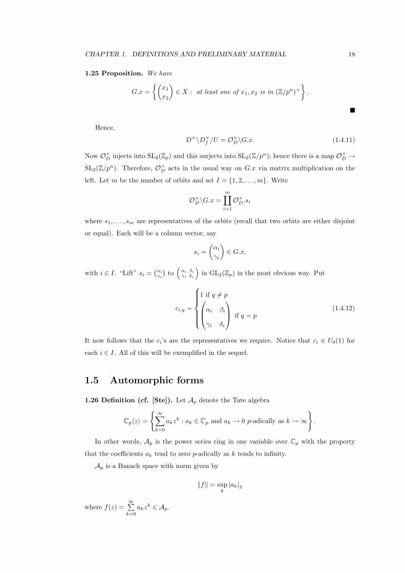
1.25 Proposition. We have

G.x ={(

x1

x2

)∈ X : at least one of x1, x2 is in (Z/pn)×

}.

�

Hence,

D×\D×f /U = O×

D\G.x. (1.4.11)

Now O×D injects into SL2(Zp) and this surjects into SL2(Z/pn); hence there is a map O×

D →

SL2(Z/pn). Therefore, O×D acts in the usual way on G.x via matrix multiplication on the

left. Let m be the number of orbits and set I = {1, 2, . . . ,m}. Write

O×D\G.x =

m∐i=1

O×D.si

where s1, . . . , sm are representatives of the orbits (recall that two orbits are either disjoint

or equal). Each will be a column vector, say

si =(

αi

γi

)∈ G.x,

with i ∈ I. “Lift” si =(αi

γi

)to(

αi βi

γi δi

)in GL2(Zp) in the most obvious way. Put

ci,q =

1 if q 6= pαi βi

γi δi

if q = p(1.4.12)

It now follows that the ci’s are the representatives we require. Notice that ci ∈ U0(1) for

each i ∈ I. All of this will be exemplified in the sequel.

1.5 Automorphic forms

1.26 Definition (cf. [Ste]). Let Ap denote the Tate algebra

Cp〈z〉 =

{ ∞∑k=0

akzk : ak ∈ Cp and ak → 0 p-adically as k → ∞

}.

In other words, Ap is the power series ring in one variable over Cp with the property

that the coefficients ak tend to zero p-adically as k tends to infinity.

Ap is a Banach space with norm given by

‖f‖ = supk

|ak|3

where f(z) =∞∑

k=0

akzk ∈ Ap.

CHAPTER 1. DEFINITIONS AND PRELIMINARY MATERIAL 19

Next, we define a monoid and an action of this monoid on Ap. We write Op to denote

the integers of Cp and mp for its maximal ideal. We assume from now on that p is an odd

prime.

1.27 Definition (cf. [Ste]). Let κ : Z×p → O×

p be a locally analytic character, i.e. a

continuous group homomorphism. Given α ∈ N, let

Σα =

γ =

a b

c d

∈ M2(Zp) : pα | c, p - d,det(γ) 6= 0

.

The weight κ action of γ =(

a bc d

)∈ Σα on Ap is given by the continuous Cp-linear extension

of the map sending

zk 7→ κ(cz + d)(cz + d)2

(az + b

cz + d

)k

(1.5.13)

and given f(z) ∈ Ap, we write (f‖κγ)(z) for this action. Note, that by κ(cz + d) we mean

the power series expansion of κ(cz + d) at zero.

It is an easy check that Σα is a monoid and that ‖κ is a right-action of Σα on Ap.

1.28 Definition. Let α belong to N and suppose that U is an open compact subgroup of

D×f . We say that U has wild level ≥ pα if the projection U → D×

p , i.e. Up, is contained in

Σα.

1.29 Remark. The terminology of Definition 1.28 is not standard.

We are now ready to define the space of automorphic forms:

1.30 Definition (cf. Section 3 of [Buzc]). Fix α ∈ N and κ as in Definition 1.27. Let

U be an open, compact subgroup of D×f of wild level ≥ pα. Let A be any right Σα-module.

The level U , weight κ space of automorphic forms is the space,

L(U,A) = {ϕ : D×f → A : ϕ(dgu) = ϕ(g)‖κup∀ d ∈ D×, g ∈ D×

f , u ∈ U}.

The main result of interest concerning L(U,A) is:

1.31 Lemma. Let U be an open compact subgroup of D×f of wild level ≥ pα and suppose

that D×f =

∐i∈I D×ciU . Then

L(U,A) ∼=⊕i∈I

AΓi

as a Cp-vector space, where Γi := c−1i D×ci ∩ U .

Proof. It is an easy check that the map L(U,A) →⊕

i∈I AΓi given by

ϕ 7→ (ϕ(ci))i∈I

is an isomorphism. Here AΓi is the subset of A that is fixed by Γi. �

CHAPTER 1. DEFINITIONS AND PRELIMINARY MATERIAL 20

1.6 Hecke operators

We are now ready to define Hecke operators. We retain the notation of previous sections.

Let U be an open compact subgroup of D×f . Fix α ∈ N and κ as in Definition 1.27.

Given ϕ ∈ L(U,A) we define a new right action of U on L(U,A): set

(ϕ|κu) (g) := ϕ(gu−1

)‖κup.

It is easily verified that this is a right action.

1.32 Definition. Let v ∈ D×f such that vp ∈ Σα. Then the double coset UvU may be

written as a disjoint union

UvU =∐t∈T

Uvt

where T is a finite set, and vt ∈ D×f . The Hecke operator is the map [UvU ] : L(U,A) →

L(U,A) given by

[UvU ]ϕ :=∑t∈T

ϕ|κvt.

Of particular interest are the standard Hecke operators defined as follows: Assume that

l is an odd prime. Define $l to be the element of Af which is l at l and 1 at all other places.

Put ηl =(

$l 00 1

), i.e. ηl is trivial at all places except at l where it is ( l 0

0 1 ).

1.33 Definition. The standard Hecke operators are given by

Tl := [UηlU ] and Sl := [U$lU ] .

If l = p, it is traditional to write Up for Tp.

We shall focus on the operators Up acting on the space L(U,Ap), where U is U0(pn) or

U1(pn). Write Up = [UηpU ] =[∐

t∈T Uvt

].

Our main interest is in the matrix of Up and our first goal is to explain how to obtain

its matrix. Consider the following diagram

L(U,Ap)ϕ 7→(ϕ(ci))i∈I−−−−−−−−−→

⊕i∈I AΓi

p

ϕ 7→(Upϕ)

y y Map ofinterest

L(U,Ap) −−−−−−−−−−−−−→Upϕ 7→((Upϕ)(ci))i∈I

⊕i∈I AΓi

p

We are interested in the vertical map on the right-hand edge of the commutative diagram,

i.e. the map⊕

i∈I AΓip to

⊕i∈I AΓi

p that sends

(ϕ(ci))i∈I → ((Upϕ)(ci))i∈I .

CHAPTER 1. DEFINITIONS AND PRELIMINARY MATERIAL 21

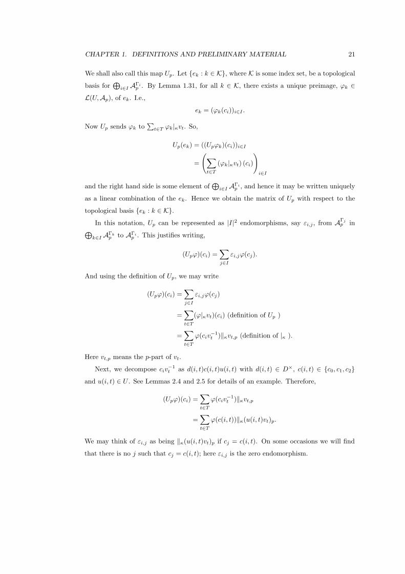
We shall also call this map Up. Let {ek : k ∈ K}, where K is some index set, be a topological

basis for⊕

i∈I AΓip . By Lemma 1.31, for all k ∈ K, there exists a unique preimage, ϕk ∈

L(U,Ap), of ek. I.e.,

ek = (ϕk(ci))i∈I .

Now Up sends ϕk to∑

t∈T ϕk|κvt. So,

Up(ek) = ((Upϕk)(ci))i∈I

=

(∑t∈T

(ϕk|κvt) (ci)

)i∈I

and the right hand side is some element of⊕

i∈I AΓip , and hence it may be written uniquely

as a linear combination of the ek. Hence we obtain the matrix of Up with respect to the

topological basis {ek : k ∈ K}.

In this notation, Up can be represented as |I|2 endomorphisms, say εi,j , from AΓjp in⊕

k∈I AΓkp to AΓi

p . This justifies writing,

(Upϕ)(ci) =∑j∈I

εi,jϕ(cj).

And using the definition of Up, we may write

(Upϕ)(ci) =∑j∈I

εi,jϕ(cj)

=∑t∈T

(ϕ|κvt)(ci) (definition of Up )

=∑t∈T

ϕ(civ−1t )‖κvt,p (definition of |κ ).

Here vt,p means the p-part of vt.

Next, we decompose civ−1t as d(i, t)c(i, t)u(i, t) with d(i, t) ∈ D×, c(i, t) ∈ {c0, c1, c2}

and u(i, t) ∈ U . See Lemmas 2.4 and 2.5 for details of an example. Therefore,

(Upϕ)(ci) =∑t∈T

ϕ(civ−1t )‖κvt,p

=∑t∈T

ϕ(c(i, t))‖κ(u(i, t)vt)p.

We may think of εi,j as being ‖κ(u(i, t)vt)p if cj = c(i, t). On some occasions we will find

that there is no j such that cj = c(i, t); here εi,j is the zero endomorphism.

Chapter 2

U3

2.1 U3 Evaluated

We work in the case p = 3 and investigate the Hecke operator U3, level U1(9). We focus on

maps κ satisfying the following properties,

1. we can write κ(4) = 4t, where t = log3(κ(4))log3(4)

.

2. v3(t) > 0, so that t ∈ m3,

3. and without loss of generality, κ(−1) = 1.

Here, A3 is simply, { ∞∑k=0

akzk : ak → 0 3-adically as k → ∞

}.

We shall be working over the ring Z3, and making use of the isomorphism θ3 of Chapter 1.

To this end, we choose our elements ν3, ξ3 of Z3 such that ν23 + ξ2

3 = −1 as follows: take ν3

to be the square root of −2 in Z3 that is 508 mod 37 and ξ3 = 1. It is readily verified that

(ν3)2 = −2. It is an easy exercise to verify that ν3 has 3-adic expansion beginning with,

ν3 = 1 + 3 + 2 · 32 + 2 · 35 + 37 + 2 · 311 + 312 + . . .

Recall that in D = Q(i, j), our maximal order OD is Z[i, j, 1

2 (1 + i + j + k)], and so

O×D = {±1,±i,±j,±k,±u1,±u2,±u3,±u4,±u5,±u6,±u7,±u8}

22

CHAPTER 2. U3 23

where

u1 = 12 (1 + i + j + k) ,

u2 = 12 (−1 + i + j + k) ,

u3 = 12 (1 − i + j + k) ,

u4 = 12 (1 + i − j + k) ,

u5 = 12 (1 + i + j − k) ,

u6 = 12 (−1 − i + j + k) ,

u7 = 12 (−1 + i − j + k) and

u8 = 12 (−1 + i + j − k) .

The details may be found in [Vig80].

Our first goal is to find coset representatives in the decomposition. We have

D×f =

∐i∈I

D×ciU1(9).

We have

2.1 Theorem.

D×f = D×c0U1(9) q D×c1U1(9) q D×c2U1(9)

where

c0,p = 1 ∀ p

c1,p =

1 if p 6= 3

( 5 00 2 ) if p = 3

c2,p =

1 if p 6= 3

( 7 00 4 ) if p = 3

Proof. Most of the hard work has been done in Chapter 1, and all we need do is to compute

the right hand side of (1.4.11); here G = SL2(Z/(9)). The image of O×D is

±1 7→ ±

1 0

0 1

, ± i 7→ ±

4 1

1 5

, ±j 7→ ±

0 −1

1 0

, ±k 7→ ±

1 5

5 8

±u1 7→ ±

3 7

8 7

, ± u2 7→ ±

2 7

8 6

, ±u3 7→ ±

8 6

7 2

, ±u4 7→ ±

3 8

7 7

±u5 7→ ±

2 2

3 8

, ± u6 7→ ±

7 6

7 1

, ±u7 7→ ±

2 8

7 6

, ±u8 7→ ±

1 2

3 7

.

CHAPTER 2. U3 24

In this case, |G.x| = 72, and an unilluminating calculation shows that O×D\G.x consists of

three elements, i.e. there are three orbits. We take I = {0, 1, 2}. Suitable representatives of

the orbits are,

s0 =(

10

), s1 =

(50

), s2 =

(70

),

and we “lift” each si:

s0 =(

10

)

1 0

0 1

, s1 =(

50

)

5 0

0 2

, s2 =(

70

)

7 0

0 4

.

We define ci as in (1.4.12), and the theorem follows. �

Our next goal is to calculate the groups Γi. Recall, that Γi = c−1i D×ci ∩ U .

2.2 Lemma. Γi = {1} for all i = 0, 1, 2.

Proof. The only place of Q where we have any control is at q = 3, where all elements of U

are of the form ( ∗ ∗0 1 ) mod 9.

Γ0 = D× ∩ U , and as U is contained in U0(1), Γ0 is a subgroup of O×D. If u ∈ U , then

u ∈ O×D and u3 ≡ ( ∗ ∗

0 1 ), and from the proof of Theorem 2.1, we see that the only possibility

for Γ0 is the trivial group.

Γ1 = c−11 D×c1 ∩ U . For u ∈ Γ1 write u = c−1

1 dc1 with d ∈ D×. It is then clear that

d ∈ O×D. Hence, u3 = ( 5 0

0 2 )−1d3 ( 5 0

0 2 ) ≡ ( 2 00 5 ) d3 ( 5 0

0 2 ) ≡ ( ∗ ∗0 1 ) mod 9. This implies that

d3 ≡ ( ∗ ∗0 1 ) mod 9, and from the proof of Theorem 2.1, we find that the only possibility for

d is d = 1. Thus, Γ1 is the trivial group.

An exactly similar argument shows that Γ2 is also trivial. �

Recall from Lemma 1.31, that L(U,A3) ∼=⊕2

i=0 AΓi3 . As Γi is trivial for all i, it follows

that

L(U,A3) ∼=2⊕

i=0

A3. (2.1.1)

We take

B1 =

ei(z)

0

0

,

0

ej(z)

0

,

0

0

ek(z)

: 0 ≤ i, j, k ∈ Z

as our topological basis for

⊕2i=0 A3, where e0(z) = 1 and eh(z) = zh for h ∈ N.

The Hecke operator U3 is defined (see Definition 1.32) as,

U3 = [Uη3U ]

where

η3,q =

1 if q 6= 33 0

0 1

if q = 3

CHAPTER 2. U3 25

We need now, to calculate the decomposition of Uη3U into a disjoint union of single cosets.

We note that η3 is trivial at all primes q 6= 3, so it suffices to prove the following elementary

result.

2.3 Lemma. Write G ={(

a bc d

)∈ GL2(Z3) :

(a bc d

)≡ ( ∗ ∗

0 1 ) mod 9}. Then,

G

3 0

0 1

G = G

3 0

0 1

q G

3 0

9 1

q G

3 0

18 1

(2.1.2)

�

Thus, we have,

Uη3U =2∐

t=0

Uvt

where vt,p = 1 if p 6= 3 and

vt,3 =

3 0

9t 1

= 2 − (ν3 + 92 tξ3)i + 9

2 tj + ( 92 tν3 − ξ3)k,

for t = 0, 1, 2.

Recall that U3 may be represented by |I|2 = 9 endomorphisms. Our goal now is to com-

pute these. From Chapter 1 we know that we may find these endomorphisms by evaluating

U3ϕ at c0, c1 and c2. Therefore,

(U3ϕ)(ci) =2∑

j=0

εi,jϕ(cj)

=2∑

t=0

(ϕ|κvt)(ci)

=2∑

t=0

ϕ(civ−1t )‖κvt,3

=2∑

t=0

ϕ(civ−1t )‖κ ( 3 0

9t 1 ) .

It will be convenient to identify an element of D×f with its 3-part whenever that element

is trivial at all other place. Thus,(

a1 b1c1 d1

)will simply refer to the element that is 1 at all

primes not equal to 3, and(

a1 b1c1 d1

)at 3; d

(a1 b1c1 d1

) (a2 b2c2 d2

)will indicate the element that is

the product of the quaternion d ∈ D×, the element that is 1 at all primes not equal to 3

and(

a1 b1c1 d1

)at 3 and the element that is 1 at all primes not equal to 3 and

(a2 b2c2 d2

)at 3.

The next step is to determine the cosets in the decomposition from Theorem 2.1 to which

each of the 9 elements civ−1t belong. We present the algorithm for solving this problem in

the form of two lemmas:

2.4 Lemma. There exists d ∈ D× such that d−1civ−1t ∈ U0(1).

CHAPTER 2. U3 26

Proof. From (1.4.4) we can write civ−1t = du. Hence, d−1 = uvtc

−1i . Taking determinants

(or what is the same thing, norms) gives us:

• Determinants at l 6= 2, 3: det(d−1

l

)= det(ul) det(vt,l) det

(c−1i,l

)∈ Z×

l

• “Determinants” i.e. norms at l = 2: det(d−12

)= N(u2)N(vt,2)N

(c−1i,2

)∈ Z×

2

• Determinants at l = 3: det(d−13

)= det(u3) det(vt,3) det

(c−1i,3

)∈ 3Z×

3

Hence, det(d−1

l

)= 3µ with µ ∈ Z×

l for all primes l. Thus µ = 1 since µ ∈⋂

l Z×l = {±1}

and since N (and det) maps D to Q≥0.

Certainly, d−1 ∈ OD,l for all primes l. So it follows that d−1 ∈ OD. So writing d−1 =

a0 +a1i+a2j+a3k gives that |ar| ≤√

3 < 1.8. Hence for r = 0, 1, 2, 3, ar ∈{0,±1

2 ,±1,± 32

}.

Next, we can write

d−13 = u3vt,3c

−1i,3

=

α β

γ δ

3 0

9t 1

ζ 0

0 θ

, say

=

3(α + 3βt)ζ βθ

3(γ + 3δt)ζ δθ

≡

0 ∗

0 ∗

mod 3

since ζ and θ are units and at least one of β and δ are units.

All that remains is to check the possibilities (see Section B.1) and we find that d−1 =

− 32 − 1

2 i − 12 j + 1

2 k, so that d = − 12 + 1

6 i + 16 j − 1

6 k. �

2.5 Lemma. Given u ∈ U0(1), there exist α ∈ O×D, i ∈ I and u ∈ U such that u = αciu.

Proof. Given such u, we can write u = αciu for some α ∈ D×, i ∈ I and u ∈ U by Theorem

2.1. But α = uu−1c−1i ∈ U0(1). So, α ∈ U0(1) ∩ D× = O×

D. �

In view of Lemma 2.5, we simply test the possibilities c−1i α−1u to see which lies in U .

From the calculations of Section B.1, which implement Lemmas 2.4 and 2.5, we find that

c0v−10 =

(− 1

3 − 13 i + 1

3 j)7 0

0 4

121ν3 − 1

2127

0 −14ν3 − 1

4

c1v−10 =

(13 + 1

3 i − 13 j)1 0

0 1

−53ν3 + 5

3 −4

0 2ν3 + 2

c2v

−10 =

(13 + 1

3 i − 13 j)5 0

0 2

− 715ν3 + 7

15 − 85

0 2ν3 + 2

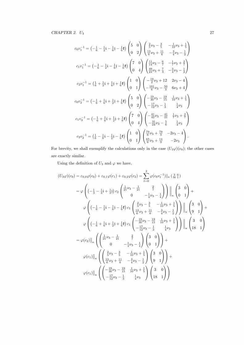
CHAPTER 2. U3 27

c0v−11 =

(−1

6 − 12 i − 1

6 j − 16 k)5 0

0 2

25ν3 − 3

5 − 110ν3 + 1

5

136 ν3 + 11

6 −34ν3 − 1

2

c1v

−11 =

(−1

6 − 12 i − 1

6 j − 16 k)7 0

0 4

1114ν3 − 6

7 − 17ν3 + 2

7

4924ν3 + 7

3 − 34ν3 − 1

2

c2v

−11 =

(16 + 1

2 i + 16 j + 1

6 k)1 0

0 1

− 192 ν3 + 12 2ν3 − 4

− 1016 ν3 − 50

3 6ν3 + 4

c0v

−12 =

(−1

6 + 16 i + 1

2 j + 16 k)5 0

0 2

−1930ν3 − 19

15110ν3 + 1

5

− 1712ν3 − 1

314ν3

c1v

−13 =

(− 1

6 + 16 i + 1

2 j + 16 k)7 0

0 4

− 4142ν3 − 41

2117ν3 + 2

7

−3124ν3 − 5

614ν3

c2v

−12 =

(16 − 1

6 i − 12 j − 1

6 k)1 0

0 1

796 ν3 + 79

3 −2ν3 − 4656 ν3 + 14

3 −2ν3

.

For brevity, we shall exemplify the calculations only in the case (U3ϕ)(c0); the other cases

are exactly similar.

Using the definition of U3 and ϕ we have,

(U3ϕ)(c0) = ε0,0ϕ(c0) + ε0,1ϕ(c1) + ε0,2ϕ(c2) =2∑

t=0

ϕ(c0v−1t )‖κ ( 3 0

9t 1 )

= ϕ

(− 13 − 1

3 i + 13 j)c2

121ν3 − 1

2127

0 −14ν3 − 1

4

∥∥∥∥κ

3 0

0 1

+

ϕ

(− 16 − 1

2 i − 16 j − 1

6 k)c1

25ν3 − 3

5 − 110ν3 + 1

5

136 ν3 + 11

6 −34ν3 − 1

2

∥∥∥∥κ

3 0

9 1

+

ϕ

(− 16 + 1

6 i + 12 j + 1

6 k)c1

− 1930ν3 − 19

15110ν3 + 1

5

−1712ν3 − 1

314ν3

∥∥∥∥κ

3 0

18 1

= ϕ(c2)

∥∥κ

121ν3 − 1

2127

0 −14ν3 − 1

4

3 0

0 1

+

ϕ(c1)∥∥

κ

25ν3 − 3

5 − 110ν3 + 1

5

136 ν3 + 11

6 − 34ν3 − 1

2

3 0

9 1

+

ϕ(c1)∥∥

κ

− 1930ν3 − 19

15110ν3 + 1

5

−1712ν3 − 1

314ν3

3 0

18 1

CHAPTER 2. U3 28

and comparing the first and last lines gives, upon simplification,

ε0,0ϕ(c0) = 0

ε0,1ϕ(c1) = ϕ(c1)∥∥

κ

( 310 ν3 − 1

10 ν3+15

− 14ν3+1 −3

4ν3−12

)+

ϕ(c1)∥∥

κ

(− 1

10 ν3−15

110 ν3+

15

14ν3−1

14ν3

)ε0,2ϕ(c2) = ϕ(c2)

∥∥κ

( 17ν3−

17

27

0 − 14ν3−

14

).

Similarly, we obtain,

ε1,0ϕ(c0) = ϕ(c1)‖κ

(−5ν3+5 −40 2ν3+2

)ε1,1ϕ(c1) = 0

ε1,2ϕ(c2) = ϕ(c2)∥∥

κ

( 1514 ν3 −1

7ν3+27

−58ν3+

52 − 3

4ν3−12

)+

ϕ(c2)∥∥

κ

(−15

14 ν3−57

17ν3+

27

58ν3−

52

14ν3

)and

ε2,0ϕ(c0) = ϕ(c0)∥∥

κ

(−21

2 ν3 2ν3−4

72ν3−14 6ν3+4

)+

ϕ(c0)∥∥

κ

( 72ν3+7 −2ν3−4

− 72ν3+14 −2ν3

)ε2,1ϕ(c1) = ϕ(c1)

∥∥κ

(−7

5ν3+75 −8

50 2ν3+2

)ε2,2ϕ(c2) = 0.

Thus, the matrix of U3 will have the form,

A =

ε0,0 ε0,1 ε0,2

ε1,0 ε1,1 ε1,2

ε2,0 ε2,1 ε2,2

=

0 ε0,1 ε0,2

ε1,0 0 ε1,2

ε2,0 ε2,1 0

noticing that εi,i = 0 for i = 1, 2, 3, which shows that the trace of U3 is zero. We shall use εi,j

to denote both the endomorphism εi,j as well as its matrix with respect to the topological

basis E1 defined below; this should not cause any confusion.

Our next aim is to calculate the generating functions of the non-zero εi,j . To this end,

and to simplify the computations, we regard each εi,j as being an endomorphism of A3,

as opposed to being an endomorphism from the j-th copy of A3 in the direct sum in the

left-hand side of (2.1.1) to the i-th copy.

Each (εk,lϕ)(cl) is a sum of things of the shape,

ϕ(ct)‖κ

(a bc d

)

CHAPTER 2. U3 29

and each of these must be treated separately. We evaluate this action on the topological

basis E1 = {er(z) : 0 ≤ r ∈ Z} of A3. From the isomorphism (2.1.1), we may assume that ϕ

is chosen such that ϕ(ct) = er(z) for some r. So now it is clear that

ϕ(ct)‖κ

(a bc d

)=(er‖κ

(a bc d

))(z) =

κ(cz + d)(cz + d)2

(az + b

cz + d

)r

and using the results of Appendix A, we can write

κ(cz + d)(cz + d)2

(az + b

cz + d

)r

=∞∑

m=0

a(r)m zm, (2.1.3)

with a(r)m ∈ C3. All that remains unclear is κ(cz + d), which may be evaluated as follows: as

a notational convenience, we shall switch to using x in place of z. In all cases of(

a bc d

)that

we will calculate with, c ≡ 0 mod 9 and d ≡ 1 mod 9. Therefore, cx+ d = 1 + 9(c′x + d′) for

some c′, d′ ∈ Z3.

Write cx + d = 4ρ, where ρ = log3(cx+d)log3(4)

. Of course ρ will be a power series in x. It

is clear that log3(cx+d)log3(4)

really does converge since cx + d = 1 + 9(c′x + d′) and log3(1 + X)

converges for |X|3 < 1. Then,

4ρ =∞∑

h=0

3h

(ρ

h

)= 1 + 3

(ρ

1

)+ 32

(ρ

2

)+ . . .

where by(

ρh

)we mean 1

h!

h−1∏k=0

(ρ − k).

Then κ(cx + d) = κ(4ρ) = κ(4)ρ = 4tρ = (4ρ)t = (cx + d)t. Lastly, we write (cx + d)t =

exp3(t log(cx + d)). A simple calculation shows that t log(cx + d) is in the radius of conver-

gence of exp3 so that exp3(t log(cx + d)) converges to an element of O3[[x]]. Thus we may

obtain a(r)m .

2.6 Proposition. The generating function of the operator ‖κ

(a bc d

)is given by

κ(cx + d)(cx + d)(cx + d − axy − by)

.

Proof. ‖κ

(a bc d

)has matrix (a(r)

m )0≤m,r∈Z, with rows indexed by m. The generating function

of ‖κ

(a bc d

)is simply

∑0≤r,m∈Z a

(r)m xmyr, and rearranging this formal sum we obtain,∑

0≤r,m∈Za(r)

m xmyr =∞∑

r=0

yr∞∑

m=0

a(r)m xm

=∞∑

r=0

yr κ(cx + d)(cx + d)2

(ax + b

cx + d

)r

using (2.1.3)

=κ(cx + d)(cx + d)2

∞∑r=0

yr

(ax + b

cx + d

)r

=κ(cx + d)(cx + d)2

1

1 − y(

ax+bcx+d

)=

κ(cx + d)(cx + d)(cx + d − axy − by)

.

CHAPTER 2. U3 30

�

It is now simply a matter of writing down the rational functions of each εk,l.

ε0,1 : h0,1(x, y) =κ((− 1

4ν3 + 1)x − 3

4ν3 − 12

) ((−1

4ν3 + 1)x − 3

4ν3 − 12

)−1(− 1

4ν3 + 1)x − 3

4ν3 − 12 − 3

10ν3xy −(− 1

10ν3 + 15

)y

+

κ((

14ν3 − 1

)x + 1

4ν3

) ((14ν3 − 1

)x + 1

4ν3

)−1(14ν3 − 1

)x + 1

4ν3 +(

110ν3 + 1

5

)xy −

(110ν3 + 1

5

)y

(2.1.4)

ε0,2 : h0,2(x, y) =κ(− 1

4ν3 − 14

) (− 1

4ν3 − 14

)−1

−14ν3 − 1

4 −(

17ν3 − 1

7

)xy − 2

7y(2.1.5)

ε1,0 : h1,0(x, y) =κ (2ν3 + 2) (2ν3 + 2)−1

2ν3 + 2 − (−5ν3 + 5) xy − 4y(2.1.6)

ε1,2 : h1,2(x, y) =κ(

58 (4 − ν3) x − 1

4 (3ν3 + 2)) (

58 (4 − ν3)x − 1

4 (3ν3 + 2))−1

58 (4 − ν3)x − 1

4 (3ν3 + 2) − 1514ν3xy + 1

7 (ν3 − 2) y+

κ(

58 (ν3 − 4)x + 1

4ν3

) (58 (ν3 − 4)x + 1

4ν3

)−1

58 (ν3 − 4)x + 1

4ν3 + 514 (ν3 + 2) xy − 1

7 (ν3 + 2) y

(2.1.7)

ε2,0 : h2,0(x, y) =κ(

72 (ν3 − 4)x + 6ν3 + 4

) (72 (ν3 − 4)x + 6ν3 + 4

)−1

72 (ν3 − 4)x + 6ν3 + 4 + 21

2 ν3xy + (4 − 2ν3) y+

κ(

72 (4 − ν3)x − 2ν3

) (72 (4 − ν3) x − 2ν3

)−1

72 (4 − ν3)x − 2ν3 − 7

2 (ν3 + 2) xy + (2ν3 + 4) y

(2.1.8)

ε2,1 : h2,1(x, y) =κ (2ν3 + 2) (2ν3 + 2)−1

2ν3 + 2 − 75 (ν3 − 1)xy − 8

5y(2.1.9)

For a given, fixed κ, we may now use either the generating functions of each εk,l or the

techniques outlined in Appendix A to obtain a formula for the (m, r)-th entry of the matrix

with respect to the topological basis E1. Hence we obtain the matrix of U3 with respect to

the topological basis B1.

2.7 Lemma. Every non-zero εk,l is compact.

Proof. Note that by definition, hk,l(x, y) ∈ O3[[x, y]]. By Corollary 1.10, it suffices to prove

that every entry in D(

13

)εk,l is in O3. Equivalently, we need to show that hk,l

(13x, y

)lies

in O3[[x, y]]. It is simply a case of checking that every coefficient of x is divisble by 3 in

O3. �

Unfortunately the topological basis B1 does not suffice to prove anything about the

slopes of the matrix of U3. As an example of this, we briefly consider the case κ(x) = x3.

(See Section B.3 for the details.) Here, the slopes of U3 were found to be

12,12,32,32,52,52, 3,

72,72,92,92, 5,

112

,112

, . . .

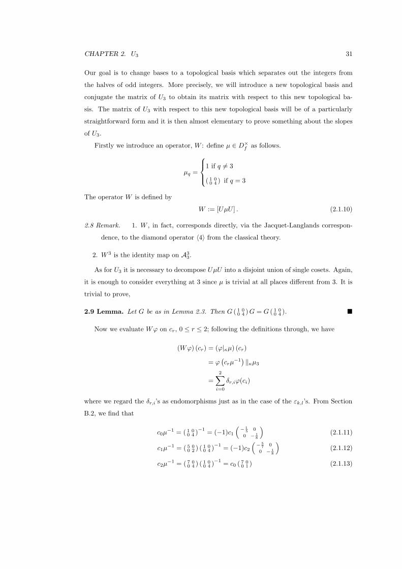
CHAPTER 2. U3 31

Our goal is to change bases to a topological basis which separates out the integers from

the halves of odd integers. More precisely, we will introduce a new topological basis and

conjugate the matrix of U3 to obtain its matrix with respect to this new topological ba-

sis. The matrix of U3 with respect to this new topological basis will be of a particularly

straightforward form and it is then almost elementary to prove something about the slopes

of U3.

Firstly we introduce an operator, W : define µ ∈ D×f as follows.

µq =

1 if q 6= 3

( 1 00 4 ) if q = 3

The operator W is defined by

W := [UµU ] . (2.1.10)

2.8 Remark. 1. W , in fact, corresponds directly, via the Jacquet-Langlands correspon-

dence, to the diamond operator 〈4〉 from the classical theory.

2. W 3 is the identity map on A33.

As for U3 it is necessary to decompose UµU into a disjoint union of single cosets. Again,

it is enough to consider everything at 3 since µ is trivial at all places different from 3. It is

trivial to prove,

2.9 Lemma. Let G be as in Lemma 2.3. Then G ( 1 00 4 ) G = G ( 1 0

0 4 ). �

Now we evaluate Wϕ on cr, 0 ≤ r ≤ 2; following the definitions through, we have

(Wϕ) (cr) = (ϕ|κµ) (cr)

= ϕ(crµ

−1)‖κµ3

=2∑

i=0

δr,iϕ(ci)

where we regard the δr,i’s as endomorphisms just as in the case of the εk,l’s. From Section

B.2, we find that

c0µ−1 = ( 1 0

0 4 )−1 = (−1)c1

(− 1

5 0

0 − 18

)(2.1.11)

c1µ−1 = ( 5 0

0 2 ) ( 1 00 4 )−1 = (−1)c2

(− 5

7 0

0 − 18

)(2.1.12)

c2µ−1 = ( 7 0

0 4 ) ( 1 00 4 )−1 = c0 ( 7 0

0 1 ) (2.1.13)

CHAPTER 2. U3 32

Recall our convention to identify an element with its 3-part if it is trivial at all other places.

Continuing, we obtain

(Wϕ) (c0) = ϕ(c1)‖κ

(− 1

5 0

0 − 12

)= δ0,1ϕ(c1)

(Wϕ) (c1) = ϕ(c2)‖κ

(− 5

7 0

0 − 12

)= δ1,2ϕ(c2)

(Wϕ) (c2) = ϕ(c0)‖κ ( 7 00 4 ) = δ2,0ϕ(c0)

so W has matrix

W =

0 δ0,1 0

0 0 δ1,2

δ2,0 0 0

Evaluating each δk,l on the elements of the topological basis E1, regarding each as an en-

domorphism of A3, we find (writing δi,j for both the endomorphism and its matrix with

respect to E1):

δ0,1 = 4κ(− 1

2

)D(

25

)δ2,0 = 4κ

(− 1

2

)D(

107

)δ0,1 = 1

16κ (4)D(

74

)

recalling the notation (1.1.2). Explicilty, the matrix of W with respect to B1 is0 4κ

(− 1

2

)D(

25

)0

0 0 4κ(−1

2

)D(

107

)116κ (4)D

(74

)0 0

Since W 3 is the identity map on A3

3, it follows from linear algebra that A33 splits into three

subspaces associated to W , namely the eigenspaces. Clearly W has minimal polynomial

F (X) = X2 + X + 1. Let ω = −1+√−3

2 ∈ C3 be a root of F (X). Let the eigenspaces of W

be K0 = ker(W − I), K1 = ker(W − ωI) and K2 = ker(W − ω2I). Now W commutes with

U3, and so U3 stabilizes each Kt. Our goal now is to choose bases for each Kt. It may be

readily verified that

• b(0)r (z) =

16κ

(14

)er

(47z)

4κ(−1

2

)er

(107 z)

er(z)

, 0 ≤ r ∈ Z, is a topological basis for K0

• b(1)r (z) =

16κ

(14

)ωer

(47z)

4κ(−1

2

)ω2er

(107 z)

er(z)

, 0 ≤ r ∈ Z, is a topological basis for K1

CHAPTER 2. U3 33

• b(2)r (z) =

16κ

(14

)ω2er

(47z)

4κ(−1

2

)ωer

(107 z)

er(z)

, 0 ≤ r ∈ Z, is a topological basis for K2

Let B2 denote the topological basis{

b(0)r (z), b(1)

s (z), b(2)t (z) : 0 ≤ r, s, t ∈ Z

}of A3

3.

It is clear the change of basis matrix is given by

B =

16κ

(14

)D(

47

)16ωκ

(14

)D(

47

)16ω2κ

(14

)D(

47

)4κ(−1

2

)D(

107

)4ω2κ

(−1

2

)D(

107

)4ωκ

(− 1

2

)D(

107

)D(1) D(1) D(1)

and moreover, B is invertible. We find that,

3B−1 =

116κ (4)D

(74

)14κ (−2)D

(710

)D(1)

116ω2κ (4)D

(74

)14ωκ (−2)D

(710

)D(1)

116ωκ (4)D

(74

)14ω2κ (−2)D

(710

)D(1)

We have,

2.10 Lemma.

B−1AB =

116κ(4) D

�74

�ε0,2+

14κ(−2) D

�710

�ε1,2

0 0

0116ω2κ(4) D

�74

�ε0,2+

14ωκ(−2) D

�710

�ε1,2

0

0 0116ωκ(4) D

�74

�ε0,2+

14ω2κ(−2) D

�710

�ε1,2

(2.1.14)

�

The proof of Lemma 2.1.14 relies heavily on a large amount of cancellation in calculation

of B−1AB; since U3 and W commute, we can easily verify the following equalities from

which all the cancellation is evident.

2.11 Lemma. The following equalities hold:

116κ(4)h0,2

(74x, y

)= 4κ

(−1

2

)h2,1

(x, 10

7 y)

= 4κ(− 1

2

)h1,0

(710x, 4

7y)

and

16κ(

14

)h2,0

(x, 4

7y)

= 14κ(−2)h1,2

(710x, y

)= 1

4κ(−2)h0,1

(74x, 10

7 y).

�

Or, bringing Proposition 1.3 into play, in terms of ε’s we have,

116κ(4)D

(74

)ε0,2 = 4κ

(−1

2

)ε2,1 D

(107

)= 4κ

(−1

2

)D(

710

)ε1,0 D

(47

)

CHAPTER 2. U3 34

and

16κ(

14

)ε2,0 D

(47

)= 1

4κ(−2)D(

710

)ε1,2 = 1

4κ(−2)D(

74

)ε0,1 D

(107

).

Set M2,2 = 116ω2κ(4)D

(74

)ε0,2 + 1

4ωκ(−2) D(

710

)ε1,2. The rational function of M2,2

is H2,2(x, y) = 116ω2κ(4)h0,2

(74x, y

)+ 1

4ωκ(−2)h1,2

(710x, y

). We shall prove that the n-th

slope of M2,2, for n ∈ N, is n − 12 . The strategy to do this is to study H2,2(x, y) in order to

verify the following.

2.12 Theorem. Suppose that M = (Mi,j)0≤i,j∈Z is an infinite matrix over O3 and is

compact. Define N = (Ni,j)0≤i,j∈Z as follows,

Ni,j :=13i

Mi,j .

If Ni,j ∈ O3 for all 0 ≤ i, j ∈ Z and det(Ni,j)0≤i,j≤n is a unit for all 0 ≤ n ∈ Z, then the

slopes of M are 0, 1, 2, 3, 4, 5, . . ..

Proof. To prove this result, we use the explicit formula for cm as given in (1.2.3). Recall

that if S is a finite subset of I = Z≥0, and σ is a permutation of S we write

MS,σ =∏i∈S

Mσ(i),i and cS =∑

σ∈Sym(S)

sgn(σ)MS,σ

Then,

cm = (−1)m∑S⊆I

|S|=m

cS . (2.1.15)

Let m ∈ N and define Sm = {0, 1, . . . ,m − 1} so that |Sm| = m. We shall prove the

following:

• v3 (cSm) = m(m−1)2 .

• v3 (MS,σ) > m(m−1)2 for all S 6= Sm such that |S| = m.

For the first point, observe that cSm is in fact the top left m×m minor of M . Write Dm(α)

to denote the diagonal matrix diag(1, α, . . . , αm−1

). The condition that det(Ni,j)0≤i,j≤n is

a unit for all n is exactly the same as saying that det(Dm

(13

))cSm is a unit for all m, or in

other words, that the valuation of det(Dm

(13

))cSm is zero. I.e.,

v3 (cSm) = v3 (det (Dm(3)))

But det (Dm(3)) = 1 · 3 · 32 · · · · · 3m−1 = 3m(m−1)

2 . Thus, we are done.

For the second point, we proceed by induction on |S|: we assume the result holds for

all S such that Sm 6= S ⊂ I and |S| = m. Let S′ = {i0 < i1 < . . . < im} be a subset of I

CHAPTER 2. U3 35

consisting of m + 1 elements and different from Sm+1. Consider v3 (MS′,σ′) where σ′ is a

permutation of S′. We have

v3 (MS′,σ′) =∑i∈S′

v3

(Mσ′(i),i

)≥∑i∈S′

σ′(i) because of the condition Ni,j ∈ O3

=∑i∈S′

i.

As S′ 6= Sm+1, there is an s′ ∈ S′ such that s′ > m + 1. Since S′ = {s′} ∪ (S′ − {s′}),

and S′ − {s′} consists of m elements, we have that∑

i∈S′−{s′} i ≥ m(m−1)2 — this is simply

the fact that the smallest possible value for the sum of m non-negative distinct integers ism(m−1)

2 . Hence,

v3 (MS′,σ′) > m + 1 +m(m − 1)

2= 1 +

m(m + 1)2

This completes the induction, except for the base case: for m = 1 we need to show that for

all S 6= S1 = {0} and |S| = 1 we have that v3(MS,σ) > 0. The conditions on S mean that

S = {s} and s ∈ N. Moreover there is only one σ — the identity permutation. It follows

that MS,σ = Ms,s and by assumption v3(Ms,s) ≥ s > 0 = 0(0−1)2 and we are done.

It now follows that v3 (cS) > m(m−1)2 for all S 6= Sm such that |S| = m since it is the

sum of things all of whose valuations are greater than 1 + m(m+1)2 .

Hence cm has valuation equal to m(m−1)2 since it is the sum of one thing that has this

valuation and other things that have strictly greater valuation. The set of “valuation co-

ordinates”, i.e. the set P = {(0, 0), (1, vp(a1)) , (2, vp(a2)) , . . .} is then,

{(0, 0), (1, 0), (2, 1), (3, 2), (4, 6), . . .}

and since these all lie on the parabola 12x(x − 1) they are on the lower boundary of a

convex polygon. Hence these are the vertices of the Newton polygon of M . The sequence

of gradients is 0, 1, 2, 3, 4, 5 . . .. I.e. the slopes are 0, 1, 2, 3, 4, 5 . . .. �

In view of Proposition 1.3, the condition of the theorem that Ni,j be in O3 is equivalent

to the statement HM

(13x, y

)∈ O3[[x, y]] where HM (x, y) is the generating function of M ;

or that the coefficient of xkyl is in 3kO3.

Recall that m3 is the maximal ideal of O3; thus the condition that det(Ni,j)0≤i,j≤n is a

unit for all 0 ≤ n ∈ Z is equivalent to det(Ni,j)0≤i,j≤n being a unit modulo m3. In other

words, the top left (n + 1) × (n + 1) minors of D(

13

)M are units for all 0 ≤ n ∈ Z.

Define M ′2,2 = 1

ω(2ω+1) D(

12ω+1

)M2,2 D(2ω + 1) — notice that this is a multiple of a

conjugate the matrix M2,2. In particular, M2,2 and D(

12ω+1

)M2,2 D(2ω + 1) will have the

same slopes because they have the same characteristic power series. To see that they have

CHAPTER 2. U3 36

have the same charateristic power series, we invoke Proposition 1.14: let u = D(

12ω+1

)M2,2

and v = D(2ω + 1). It is obvious that v is compact. For u, we examine the definition of u:

u = D(

12ω+1

) (116ω2κ(4)D

(74

)ε0,2 + 1

4ωκ(−2)D(

710

)ε1,2

)Since infinite diagonal matrices commute, we may write

u = 116ω2κ(4) D

(74

)D(

12ω+1

)ε0,2 + 1

4ωκ(−2)D(

710

)D(

12ω+1

)ε1,2

and compactness of u now follows from the proof of Lemma 2.7, since u is the sum of two

compact operators.

As the slopes are merely the valuations of the inverses of the eigenvalues of M2,2, the

presence of the multipicative factor of 1ω(2ω+1) in the definition of M ′

2,2 will simply have the

effect of adding v3 (ω(2ω + 1)) = 12 to each slope.

The rational function of M ′2,2 is then H ′

2,2(x, y) := 1ω(2ω+1)H2,2

(x

2ω+1 , y(2ω + 1)).

2.13 Lemma. H ′2,2

(13x, y

)is an element of O3[[x, y]].

Proof. This is a highly unilluminating check on the coefficients. The result will follow from

our proof of Theorem 2.14 below. �

The final step is to show that det(Ni,j)0≤i,j≤n is a unit modulo m3 for all 0 ≤ n ∈ Z,

where N = D(

13

)M ′

2,2. To do this, we study the rational function of N ; this is simply

H ′2,2

(13x, y

).

2.14 Theorem.

H ′2,2

(13x, y

)≡ −1

1 − xymod m3.

2.15 Corollary. N ≡ −D(1) mod m3.

Proof. This is merely a restatement of Theorem 2.14 in terms of matrices, via Proposition

1.3. �

Proof of Theorem 2.14. The only way to analyse this rational function is to look explicitly

CHAPTER 2. U3 37

at the numerator and denominator. The numerator is the sum of(− 2420208ωy2x4 − 26622288ων3y

2x4 + 14000231ωx4 − 46118408ων3x4+

52706752ωyx4 + 8000132ων3yx4 + 16000264ν3yx4 + 105413504yx4+

116169984ωy2x3 − 66382848ων3y2x3 − 132765696ν3y

2x3 + 232339968y2x3+

316240512ωx3 + 48000792ων3x3 + 96001584ν3x

3 − 38723328ωyx3−

425956608ων3yx3 + 632481024x3 − 768144384ωy2x2 − 128024064ων3y2x2+

435637440ωx2 − 1089093600ων3x2 + 647232768ωyx2 − 273829248ων3yx2−

547658496ν3yx2 + 1294465536yx2 − 146313216ωy2x − 438939648ων3y2x−

877879296ν3y2x − 292626432y2x + 945955584ωx + 323616384ων3x+

647232768ν3x − 1450939392ωyx − 341397504ων3yx + 1891911168x−

564350976ωy2 + 188116992ων3y2 + 448084224ω − 384072192ων3−

402361344ων3y − 804722688ν3y))κ(−ν3 − 1),

and (− 49787136ωy2x3 − 99574272ων3y

2x3 − 49787136ν3y2x3−

24893568y2x3 − 58084992ν3yx3 + 101648736yx3 − 512096256ν3y2x2+

768144384y2x2 − 261382464ν3x2 − 1642975488ωyx2 − 597445632ων3yx2−

298722816ν3yx2 − 821487744yx2 − 130691232x2 − 3072577536ωy2x−

877879296ων3y2x − 438939648ν3y

2x − 1536288768y2x − 2688505344ωx+

896168448ων3x + 448084224ν3x − 4096770048ν3yx + 896168448yx−

1344252672x − 1755758592ν3y2 − 250822656y2 − 2560481280ν3−

7461974016ωy + 877879296ων3y + 438939648ν3y − 3730987008y−

2176409088)κ(

772 (2ω + 1)x(ν3 − 4) − ν3

2

)and (

− 82978560ωy2x3 − 16595712ων3y2x3 − 8297856ν3y

2x3−

41489280y2x3 − 58084992ν3yx3 + 101648736yx3 − 256048128ν3y2x2−

256048128y2x2 − 261382464ν3x2 − 746807040ωyx2 − 149361408ων3yx2−

74680704ν3yx2 − 373403520yx2 − 130691232x2 − 146313216ωy2x+

731566080ων3y2x + 365783040ν3y

2x − 73156608y2x − 896168448ωx−

256048128ν3yx + 128024064yx − 448084224x − 752467968y2−

256048128ν3 + 146313216ωy + 146313216ων3y + 73156608ν3y+

73156608y + 128024064)κ(− 7

72 (2ω + 1)x(ν3 − 4) + 12 (3ν3 + 2)

)

CHAPTER 2. U3 38

and the denominator is

4840416ωy3x5 + 53244576ων3y3x5 + 26622288ν3y

3x5 + 2420208y3x5−

24000396ν3y2x5 − 158120256y2x5 − 28000462ωyx5 + 92236816ων3yx5+

46118408ν3yx5 − 14000231yx5 + 298722816ν3y3x4 − 522764928y3x4+

546967008ωy2x4 + 1311752736ων3y2x4 + 655876368ν3y

2x4+

273483504y2x4 + 340946802ωx4 + 148237740ων3x4 + 74118870ν3x

4+

258357204ν3yx4 − 1567084680yx4 + 170473401x4 + 3243276288ωy3x3+

597445632ων3y3x3 + 298722816ν3y

3x3 + 1621638144y3x3+

3310844544ν3y2x3 − 4281693696y2x3 + 1753440696ν3x

3+

4124034432ωyx3 + 5372861760ων3yx3 + 2686430880ν3yx3+

2062017216yx3 − 1524731040x3 + 4389396480ν3y3x2 + 2194698240y3x2+

13655900160ωy2x2 + 426746880ων3y2x2 + 213373440ν3y

2x2+

6827950080y2x2 + 7841473920ωx2 + 3920736960ων3x2 + 1960368480ν3x

2+

5974456320ν3yx2 − 10455298560yx2 + 3920736960x2 + 6145155072ωy3x−

4389396480ων3y3x − 2194698240ν3y

3x + 3072577536y3x+

7791178752ν3y2x + 8339853312y2x + 4704884352ν3x + 6785275392ωyx+

4352818176ων3yx + 2176409088ν3yx + 3392637696yx − 6721263360x+

1289945088ν3y3 + 3224862720y3 + 5141864448ωy2 − 5392687104ων3y

2−

2696343552ν3y2 + 2570932224y2 + 2176409088ω + 2560481280ων3+

1280240640ν3 + 987614208ν3y + 658409472y + 1088204544

Notice that even though all of the integers in the coefficients of the numerator and denomi-

nator are all of roughly the same order, both lie in O3[x, y]. We have not reduced modulo

anything as yet.

The next step is the evaluation of κ at −ν3 − 1, 772 (2ω + 1)x(ν3 − 4)− ν3

2 and − 772 (2ω +

1)x(ν3 − 4) + 12 (3ν3 + 2). Recall that we fixed t ∈ m3 such that κ(4) = 4t and we showed

above that κ(cx + d) = (cx + d)t where by (cx + d)t we mean exp3 (t log3 (cx + d)).

For the case, −ν3 − 1, we have −ν3 − 1 = 1 + (−2 − ν3) and −2 − ν3 ≡ 0 mod 3. Thus,

log3 (−ν3 − 1) = 3 + 9L0 with L0 ∈ Z×3 . Then, v3 (t log3 (−ν3 − 1)) = v3(t) + 1 > 1, so that

t log3 (−ν3 − 1) is in the disc of convergence of exp3. Hence exp3 (t(3 + 9L0)) converges to

an element 1 + (2ω + 1)tL1 with L1 ∈ O3. This follows from examining the power series

expansions of exp3 and noting that −3 = (2ω + 1)2

For the cases of 772 (2ω+1)x(ν3−4)− ν3

2 and − 772 (2ω+1)x(ν3−4)+ 1

2 (3ν3 +2), note that

each is of the form cx+d and that v3(c) = 12 and v3(d−1) = 1. So log3 (cx + d) converges to

CHAPTER 2. U3 39

a convergent power series in O3[[x]] in which every coefficient has valuation at least 12 . Thus,

log3 (cx + d) ∈ (2ω + 1)O3[[x]]. Multiplying by t gives an element of (2ω + 1)tO3[[x]] and

exponentiating gives an element of 1+(2ω+1)tO3[[x]]. Notice that tO3 ⊂ m3 since v3(t) > 0

and therefore 1+(2ω+1)tO3[[x]] ⊂ 1+m3[[x]]. Put κ(

772 (2ω + 1)x(ν3 − 4) − ν3

2

)= 1+(2ω+

1)tL2 and κ(− 7

72 (2ω + 1)x(ν3 − 4) + 12 (3ν3 + 2)

)= 1 + (2ω + 1)tL3 with L2, L3 ∈ O3[[x]].

The next step is to divide out all common powers of 3 from the numerator and denomi-

nators. We make the substitution ν3 = 2695+310S for S ∈ Z×3 . We find that the numerator

may be written as

36(−(2ω + 1)(x2y2 + xy + 1) + t(2ω + 1)L1(x2y2 + xy + 1)+

t(2ω + 1)L2(x2y2 + xy + 1) + t(2ω + 1)L3(x2y2 + xy + 1))

+ 37L4

for some L4 ∈ O3[[x, y]] and the denominator may be written as

36(−(2ω + 1)x3y3 + 2ω + 1

)+ 37L5

for some L5 ∈ O3[[x, y]]. Dividing out by 36(2ω + 1) gives(−(x2y2 + xy + 1) + tL1(x2y2 + xy + 1)+

tL2(x2y2 + xy + 1) + tL3(x2y2 + xy + 1))− (2ω + 1)L4

for the numerator and (1 − x3y3

)− (2ω + 1)L5

for the denominator. Modulo m3 (recalling that t, 2ω + 1 ∈ m3) the quotient becomes,

−(x2y2 + xy + 1)1 − x3y3

which is formally equal to−1

1 − xy.

�

2.16 Corollary. The n-th slope of M2,2 is n − 12 for n ∈ N.

Proof. Apply Theorem 2.14 with M = M ′2,2. �

2.2 Extending the Results

For our main example we focused on maps κ in one particular disc in weight space. It is not

too much more effort to prove similar results for the following class of κ’s

1. κ(4) = 4t+λ, where t + λ = log3(κ(4))log3(4)

for λ ∈ {1, 2},

2. v3(t) > 0, so that t ∈ m3,

CHAPTER 2. U3 40

3. and without loss of generality, κ(−1) = 1.

For each λ, this collection is another disc in weight space.

All that differs in these cases is the evaluation of (cx + d)t+λ which we regard as being

(cx + d)λ exp3 (t log3(cx + d)) and the evaluation of the exponential is as above.

Let M3,3 = 116ωκ(4) D

(74

)ε0,2 + 1

4ω2κ(−2)D(

710

)ε1,2 (see equation (2.1.14)). A similar

analysis to that applied to M2,2 will prove that the n-th slope of M3,3 is also n− 12 for n ∈ N.

Again we may extend even more to the additional κ’s detailed above.

The most obvious way to extend the results is consider other odd primes p. However, as

p increases, so does the number of cosets in the decomposition UηpU — see Definitions 1.32

and 1.33. In fact, for U = U0(pn) and U = U1(pn) there will be exactly p cosets.

We could also consider automorphic forms over a definite quaternion algebra over a

totally real field F other than Q — the so-called Hilbert case, since the automorphic forms

correspond to Hilbert Modular Forms. In this case we would have to consider operators Up

for a prime ideal p of F .

Conclusion

We began introducing the notion of an infinite matrix. Such matrices arise for example

as linear maps on Banach space. This led us to reviewing some of the theory of compact

operators on Banach spaces, and gave the definition of the characteristic power series — a

certain power series associated to each compact operator.

We next introduced the notion of the Newton polygon of a characteristic power series and

the slopes of the Newton polygon. The slopes of the Newton polygon give us information

about the valuations of the eigenvalues of a compact operator.

Next, we set up the ground work in order to define automorphic forms over a definite

quaternion algebra over Q forming the “adelic quaternion” ring,

Df = D ⊗Q Af .

Given a Cp-vector space, A, our space of automorphic forms was defined as a set of maps

D×f → A satisfying certain transformation properties.

The next step was to define a certain kind of operator, called a Hecke operator, on this

space. We focused on a particular Hecke operator U3 and a particular case of the maps κ —

the weight of the operator. By studying the rational function of this operator on a certain

subspace of the automorphic forms, we proved that the sequence of slopes of U3 on that

subspace is12,32,52,72,92,112

,132

,152

,172

,192

,212

,232

, . . .

namely it is a sequence in arithmetic progression.

41

Appendix A

Power series calculations

In this appendix, we detail some of the rather elementary, but nonetheless important formu-

lae concerning the coefficients of a formal power series which is the evolution of the quotient

or product of two polynomials in one variable.

In other terms, given M,N ∈ Z, and P,Q,R, S in some field of characteristic zero, K,

we wish to determine the coefficients am in the formal expansion,

(P + Qz)M (R + Sz)N =∞∑

m=0

amzm. (A.0.1)

To this end, we have:

A.1 Theorem. For fixed 0 ≤ m ∈ Z, dm

dzm

((P + Qz)M (R + Sz)N

), the m-th formal deriva-

tive of (P + Qz)M (R + Sz)N , is given by

1. if M > 0 and N > 0,

m∑n=0

((m

n

)(m−n−1∏q=0

(M − q)

)(n−1∏q=0

(N − q)

)×

Qm−nSn(P + Qz)M−m+n(R + Sz)N−n

)

2. if M 6= 0 and N = 0, (m−1∏q=0

(M − q)

)Qm(P + Qz)M−m

3. if M > 0 and N < 0,

m∑n=0

((−1)n

(m

n

)(m−n−1∏q=0

(M − q)

)(n−1∏q=0

(q − N)

)×

Qm−nSn(P + Qz)M−m+n(R + Sz)N−n

)

42

APPENDIX A. POWER SERIES CALCULATIONS 43

4. if M < 0 and N < 0,

m∑n=0

((−1)n

(m

n

)(m−n−1∏q=0

(q − M)

)(n−1∏q=0

(q − N)

)×

Qm−nSn(P + Qz)M−m+n(R + Sz)N−n

)

�

All of these results are easily proved using induction on m.

It is evident that the m-th formal derivative of the right hand side of equation (A.0.1) is

m!am + z × (some power series)

and evaluating both sides at z = 0 gives

A.2 Corollary. We have,

1. if M > 0 and N > 0,

am =

m∑

n=0

((M

m−n

)(Nn

)PM−m+nQm−nRN−nSn

), 0 ≤ m ≤ M + N,

0, m > M + N

2. if M 6= 0 and N = 0,

am =

(Mm

)PM−mQm if M > 0

(−1)m(−M

m

)PM−mQm if M < 0.

3. if M > 0 and N < 0,

am =m∑

n=max(0,m−M)

((−1)n

(M

m − n

)(−N

n

)PM−m+nQm−nRN−nSn

)

4. if M < 0 and N < 0,

am = (−1)mm∑

n=0

((−M

m − n

)(−N

n

)PM−m+nQm−nRN−nSn

)

�

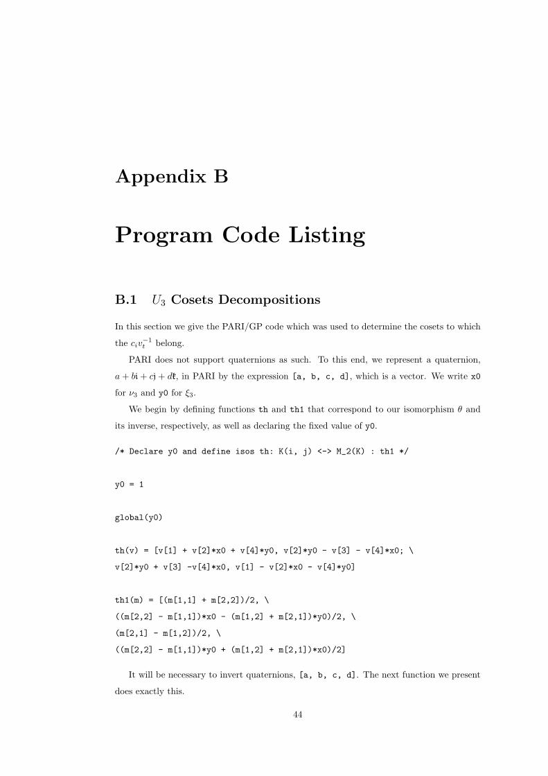
Appendix B

Program Code Listing

B.1 U3 Cosets Decompositions

In this section we give the PARI/GP code which was used to determine the cosets to which

the civ−1t belong.

PARI does not support quaternions as such. To this end, we represent a quaternion,

a + bi + cj + dk, in PARI by the expression [a, b, c, d], which is a vector. We write x0

for ν3 and y0 for ξ3.

We begin by defining functions th and th1 that correspond to our isomorphism θ and

its inverse, respectively, as well as declaring the fixed value of y0.

/* Declare y0 and define isos th: K(i, j) <-> M_2(K) : th1 */

y0 = 1

global(y0)

th(v) = [v[1] + v[2]*x0 + v[4]*y0, v[2]*y0 - v[3] - v[4]*x0; \

v[2]*y0 + v[3] -v[4]*x0, v[1] - v[2]*x0 - v[4]*y0]

th1(m) = [(m[1,1] + m[2,2])/2, \

((m[2,2] - m[1,1])*x0 - (m[1,2] + m[2,1])*y0)/2, \

(m[2,1] - m[1,2])/2, \

((m[2,2] - m[1,1])*y0 + (m[1,2] + m[2,1])*x0)/2]

It will be necessary to invert quaternions, [a, b, c, d]. The next function we present

does exactly this.

44

APPENDIX B. PROGRAM CODE LISTING 45

/* Return the inverse of the "quaternion" [q0, q1, q2, q3] */

quatinv(v) = vv = v; N = sum(ii=1, 4, v[ii]^2); \

for(ii=2,4, vv[ii] *= -1/N); vv[1] /= N; vv

The next section of code explicitly performs the computations of Lemma 2.4, i.e. it

produces a d−1 satisfying the conditions derived in Lemma 2.4.

/* Lists d1 in O_D s.t. N(d1) = 3 & d1 = [0, *; 0, *] mod 3: */

d1list=[]

forstep(d0=-2, 2, 1/2, forstep(d1=-2, 2, 1/2, \

forstep(d2=-2, 2, 1/2, forstep(d3=-2, 2, 1/2, \

if(d0^2 + d1^2 + d2^2 + d3^2 == 3, \

mm = subst(th([d0, d1, d2, d3]), x0, sqrt(-2 + O(3^15))); \

if((mm[1, 1]%3 == 0) && (mm[2, 1]%3 == 0), \

d1list = concat(d1list, [[d0, d1, d2, d3]])))))))

Here, we compute the units of OD and their matrix forms under the isomorphism θ.

/* Calculate the units of O_D & matrix versions under th: */

unitlist = []

forstep(a=-2, 2, 1/2, forstep(b=-2, 2, 1/2, \

forstep(cc=-2, 2, 1/2, forstep(d=-2, 2, 1/2, \

if(a^2 + b^2 + cc^2 + d^2 == 1, \

unitlist = concat(unitlist, [[a, b, cc, d]]))))))

matunitlist = vector(length(unitlist), i, th(unitlist[i]))

The function test determines if a given matrix mm has entries in Z3.

/* "test" tests matrices for integral entries: */

test(mm) = MM = mm; temp = matrix(2, 2, i, j, \

valuation(MM[i,j], 3)); mmin = vecmin([vecmin(temp[1,]), \

vecmin(temp[2,])]); mmin >= 0

Finally we can begin the decomposition calculations. The next block of code calculates

the decomposition of Lemma 2.4:

APPENDIX B. PROGRAM CODE LISTING 46

/* Step 1 Factorisation: write c_i v_t^{-1} = du: */

clist = [[1, 0; 0, 1], [5, 0; 0, 2], [7, 0; 0, 4]]

c(i) = clist[i+1]

vt3(t) = [3, 0; 9*t, 1]

fact1list = []

for(t = 0, 2, for(i = 0, 2, for(j=1, length(d1list),\

u = th(d1list[j])*c(i)*(1/vt3(t)); \

uu = subst(u, x0, sqrt(-2 + O(3^15))); \

if(test(uu), fact1list = concat(fact1list,\

[[t, i, j,[quatinv(d1list[j]), u]]]); break(1)))))

The output from this code is:

/* Output of fact1list: */

for(i=1, length(fact1list), print(fact1list[i]))

[0, 0, 1, [[-1/2, 1/6, 1/6, -1/6], \

[-1/6*x0 - 1/3, -1/2*x0; -1/6*x0 - 1/3, 1/2*x0 - 2]]]

[0, 1, 1, [[-1/2, 1/6, 1/6, -1/6], \

[-5/6*x0 - 5/3, -x0; -5/6*x0 - 5/3, x0 - 4]]]

[0, 2, 1, [[-1/2, 1/6, 1/6, -1/6], \

[-7/6*x0 - 7/3, -2*x0; -7/6*x0 - 7/3, 2*x0 - 8]]]

[1, 0, 1, [[-1/2, 1/6, 1/6, -1/6], \

[4/3*x0 - 1/3, -1/2*x0; -5/3*x0 + 17/3, 1/2*x0 - 2]]]

[1, 1, 1, [[-1/2, 1/6, 1/6, -1/6], \

[13/6*x0 - 5/3, -x0; -23/6*x0 + 31/3, x0 - 4]]]

[1, 2, 1, [[-1/2, 1/6, 1/6, -1/6], \

[29/6*x0 - 7/3, -2*x0; -43/6*x0 + 65/3, 2*x0 - 8]]]

[2, 0, 1, [[-1/2, 1/6, 1/6, -1/6], \

[17/6*x0 - 1/3, -1/2*x0; -19/6*x0 + 35/3, 1/2*x0 - 2]]]

[2, 1, 1, [[-1/2, 1/6, 1/6, -1/6], \

[31/6*x0 - 5/3, -x0; -41/6*x0 + 67/3, x0 - 4]]]

[2, 2, 1, [[-1/2, 1/6, 1/6, -1/6], \

[65/6*x0 - 7/3, -2*x0; -79/6*x0 + 137/3, 2*x0 - 8]]]

APPENDIX B. PROGRAM CODE LISTING 47

The form of the output is

[t, i, 1, [[a, b, c, d], \

[p, q; r, s]]]

meaning that (civ−1t )3 has the form (a + bi + cj + dk) ( p q

r s ); here we mix quaternion and

matrix notation. The output is easier to read in this form.

This piece of code test the factorizations:

/* Testing the factorizations: */

for(i=1, length(fact1list), mmmm = fact1list[i]; \

print1(Mod(c(mmmm[2])*(1/vt3(mmmm[1])) - \

th(mmmm[4][1])*mmmm[4][2], x0^2 + 2) "; "))

Next, we calculate the decomposition of Lemma 2.5. Here we simply test all the possibilites;

there are 3 for i and 24 for alpha:

/* Find alpha & c_i s.t. c_i^{-1} alpha^{-1} u \in U_1(9): */

D = [-1/2, 1/6, 1/6, -1/6]

fl = []

for(i=1, 9, u3 = fact1list[i][4][2]; for(ii=0, 2, \

for(jj = 1, length(matunitlist), \

v3 = (1/c(ii))*(1/matunitlist[jj])*u3; \

vv33 = subst(v3, x0, sqrt(-2 + O(3^15))); vv33 %= 9; \

if((vv33[2, 1] == 0) && (vv33[2, 2] == 1), \

fl = concat(fl, [[D, matunitlist[jj], c(ii), v3]])))))

The following is modified output of the above and gives the factorizations of the civ−1t

in the following order: c0v−10 , c1v

−10 , c2v

−10 , c0v

−11 , c1v

−11 , c2v

−11 , c0v

−12 , c1v

−12 , c2v

−12 .

/* Output: */

for(i=1, length(flX2), print(flX2[i]))

[[-1/3, -1/3, 1/3, 0], [7, 0; 0, 4], \

[1/21*X - 1/21, 2/7; 0, -1/4*X - 1/4]]

[[1/3, 1/3, -1/3, 0], [1, 0; 0, 1], \

[-5/3*X + 5/3, -4; 0, 2*X + 2]]

[[1/3, 1/3, -1/3, 0], [5, 0; 0, 2], \

APPENDIX B. PROGRAM CODE LISTING 48

[-7/15*X + 7/15, -8/5; 0, 2*X + 2]]

[[-1/6, -1/2, -1/6, -1/6], [5, 0; 0, 2], \

[2/5*X - 3/5, -1/10*X + 1/5; 13/6*X + 11/6, -3/4*X - 1/2]]

[[-1/6, -1/2, -1/6, -1/6], [7, 0; 0, 4], \

[11/14*X - 6/7, -1/7*X + 2/7; 49/24*X + 7/3, -3/4*X - 1/2]]

[[1/6, 1/2, 1/6, 1/6], [1, 0; 0, 1], \

[-19/2*X + 12, 2*X - 4; -101/6*X - 50/3, 6*X + 4]]

[[-1/6, 1/6, 1/2, 1/6], [5, 0; 0, 2], \

[-19/30*X - 19/15, 1/10*X + 1/5; -17/12*X - 1/3, 1/4*X]]

[[-1/6, 1/6, 1/2, 1/6], [7, 0; 0, 4], \

[-41/42*X - 41/21, 1/7*X + 2/7; -31/24*X - 5/6, 1/4*X]]

[[1/6, -1/6, -1/2, -1/6], [1, 0; 0, 1], \

[79/6*X + 79/3, -2*X - 4; 65/6*X + 14/3, -2*X]]

The output is of the form

[[a, b, c, d], [e, f; g, h], \

[p, q; r, s]]

and means that the corresponding (civ−1t )3 factorizes as

(a + bi + cj + dk)

e f

g h

p q

r s

.

B.2 W Cosets Decompositions

In this section we present the code for the factorizations in (2.1.11). We note at once that

ciµ−1 ∈ U0(1) for i = 0, 1, 2, so that all we require is the last step in the factorization.

All the set-up for these calculations is the same as in Section B.1, and so we omit it.

/* Step 2 Factorization: Find alpha \in O_D^\times, c_i (i \in {0, 1, 2})

s.t. c_i^{-1} alpha^{-1} c_r \eta^{-1} \in U_1(9): */

clist = [[1, 0; 0, 1], [5, 0; 0, 2], [7, 0; 0, 4]]

c(i) = clist[i+1]

cre3(r) = c(r)*[1, 0; 0, 1/4]

fl = []

APPENDIX B. PROGRAM CODE LISTING 49

for(i = 0, 2, for(jj = 1, length(unitlist), for(r = 0, 2, \

v3 = (1/c(i))*(1/th(unitlist[jj]))*cre3(r); \

vv3 = subst(v3, x0, sqrt(-2 + O(3^15))); \

if(test(vv3) && (vv3[2, 1]%9 == 0) && (vv3[2, 2]%9 == 1), \

fl = concat(fl, [[jj, i, r, [cre3(r)], [unitlist[jj], c(i), v3]]])))))

This section of code simply tests the possibilities c−1i α−1crη

−1 for fixed r ∈ {0, 1, 2}, and

varying i ∈ {0, 1, 2} and varying α ∈ O×D and determines which lies in U1(9); thus we obtain

the factorization. The output from this code is as follows:

/* Output: */

for(i=1, length(fl), print(fl[i]))

[24, 0, 2, [[7, 0; 0, 1]], [[1, 0, 0, 0], \

[1, 0; 0, 1], [7, 0; 0, 1]]]

[1, 1, 0, [[1, 0; 0, 1/4]], [[-1, 0, 0, 0], \

[5, 0; 0, 2], [-1/5, 0; 0, -1/8]]]

[1, 2, 1, [[5, 0; 0, 1/2]], [[-1, 0, 0, 0], \

[7, 0; 0, 4], [-5/7, 0; 0, -1/8]]]

The output is in the form

[a, b, c, [[a11, a12; a21, a22]], [[v1, v2, v3, v4], \

[n11, n12; n21, n22], [u11, u12; u21, u22]]]

indicating that the matrix a11 a12

a21 a22

factorizes as

(v1 + v2i + v3j + v4k)

n11 n12

n21 n22

u11 u12

u21 u22

.

The a, b and c may be ignored here.

B.3 Calculations for U3 with κ(x) = x3.

Here we give all the calculations for U3 with κ(x) = x3.

We begin by initialising the memory allocation of the PARI process and defining functions

hij(x, y, k) where i6=j take the values 0, 1, 2; these correspond to our rational functions

for the εi,j for the case of κ(x) = xk.

APPENDIX B. PROGRAM CODE LISTING 50

allocatemem(1024000000)

h02(x, y, k) = (-(x3/4) - 1/4)^(k - 1)/(-(x3/4) - 1/4 - \

(x3/7 - 1/7)*x*y - (2*y)/7)

h01(x, y, k) = ((-(x3/4) + 1)*x - (3*x3)/4 - 1/2)^(k - 1)/ \

((-(x3/4) + 1)*x - (3*x3)/4 - 1/2 - (3*x3*x*y)/10 - (-(x3/10) + 1/5)*y) + \

((x3/4 - 1)*x + x3/4)^(k - 1)/((x3/4 - 1)*x + x3/4 + (x3/10 + 1/5)*x*y - \

(x3/10 + 1/5)*y)

h10(x, y, k) = (2*x3 + 2)^(k - 1)/(2*x3 + 2 - (-5*x3 + 5)*x*y + 4*y)

h12(x, y, k) = (5/8*(4 - x3)*x - 1/4*(3*x3 + 2))^(k - 1)/ \

(5/8*(4 - x3)*x - 1/4*(3*x3 + 2) - (15*x3*x*y)/14 + 1/7*(x3 - 2)*y) + \

(5/8*(x3 - 4)*x + x3/4)^(k - 1)/(5/8*(x3 - 4)*x + x3/4 + \

5/14*(x3 + 2)*x*y - 1/7*(x3 + 2)*y)

h21(x, y, k) = (2*x3 + 2)^(k - 1)/(2*x3 + 2 + 7/5*(x3 - 1)*x*y + (8*y)/5)

h20(x, y, k) = (7/2*(x3 - 4)*x + 6*x3 + 4)^(k - 1)/ \

(7/2*(x3 - 4)*x + 6*x3 + 4 + (21*x3*x*y)/2 + (4 - 2*x3)*y) + \

(7/2*(4 - x3)*x - 2*x3)^(k - 1)/(7/2*(4 - x3)*x - 2*x3 - \

7/2*(x3 + 2)*x*y + (2*x3 + 4)*y)

Next we compute the matrices corresponding to each rational function. We omit this

output for brevity’s sake.

m02 = matrix(6, 6, i, j, (polcoeff(polcoeff(h13(x, y, 3) + \

O(x^10), i-1, x) + O(y^10), j-1, y))%(x3^2 + 2));

m01 = matrix(6, 6, i, j, (polcoeff(polcoeff(h12(x, y, 3) + \

O(x^10), i-1, x) + O(y^10), j-1, y))%(x3^2 + 2));

m10 = matrix(6, 6, i, j, (polcoeff(polcoeff(h21(x, y, 3) + \

O(x^10), i-1, x) + O(y^10), j-1, y))%(x3^2 + 2));

m12 = matrix(6, 6, i, j, (polcoeff(polcoeff(h23(x, y, 3) + \

O(x^10), i-1, x) + O(y^10), j-1, y))%(x3^2 + 2));

m21 = matrix(6, 6, i, j, (polcoeff(polcoeff(h32(x, y, 3) + \

O(x^10), i-1, x) + O(y^10), j-1, y))%(x3^2 + 2));

m20 = matrix(6, 6, i, j, (polcoeff(polcoeff(h31(x, y, 3) + \

APPENDIX B. PROGRAM CODE LISTING 51

O(x^10), i-1, x) + O(y^10), j-1, y))%(x3^2 + 2));

Next, we form the matrix of U3, which we call A

zero = matrix(6, 6, i, j, 0)

r1 = mattranspose(concat(concat(zero, m01), m02))

r2 = mattranspose(concat(concat(m10, zero), m12))

r3 = mattranspose(concat(concat(m20, m21), zero))

A = mattranspose(concat(r1, concat(r2, r3)))

We calculate the “characteristic power series” of this finite 18 × 18 matrix, A. Note that it

really does make sense to consider such finite truncations of the matrices of such operators

in view of Proposition 1.12, part 3. Next we set

x3 = sqrt(-2 + O(3^200))

— the 3-adic approximation to the√−2 ∈ Z3, and then compute

l = matdet(A - t*matid(18));

and the slopes of this are calculated as follows:

newtonpoly(l, 3)

The output of this is

[2147483647, 2147483647, 12, 8, 11/2, 11/2, 5, 9/2, 9/2, 7/2, 7/2, 3, \

5/2, 5/2, 3/2, 3/2, 1/2, 1/2]

The output is presented in reverse to our definition in Chapter 1.

Bibliography

[AB95] J. L. Alperin and R. B. Bell. Groups and Representations. Number 162 in GTM.

Springer, 1995.

[Bur97] D. M. Burton. Elementary Number Theory. McGraw-Hill, fourth edition, 1997.

[Buza] K. M. Buzzard. Eigencurves for automorphic forms. Work in progress.

[Buzb] K. M. Buzzard. Eigenvarieties. Work in progress.

[Buzc] K. M. Buzzard. On p-adic families of automorphic forms. This has been

submitted to the Barcelona 2002 conference proceedings; preprint available at

http://www.ma.ic.ac.uk/∼kbuzzard/maths/research/papers/index.html.

[Cas95] J. W. S. Cassels. Local Fields, volume 3 of London Mathematical Society Student

Texts. Cambridge University Press, 1995.

[CF67] J. W. S. Cassels and A. Frohlich, editors. Algebraic Number Theory. Academic

Press, 1967.

[Col97] R. Coleman. p-adic Banach Spaces and Families of Modular Forms. Inventiones

Mathematicae, 127:417–479, 1997.

[CST98] R. Coleman, G. Stevens, and J. Teitelbaum. Numerical Experiments on Families

of p-adic Modular Forms. AMS/IP Studies in Advanced Mathematics, 7:143–158,

1998.

[DT94] F. Diamond and R. Taylor. Non-optimal levels of mod l modular representations.

Invent. Math., 115:435–462, 1994.

[Dwo62] B. Dwork. On the Zeta Function of a Hypersurface. Inst. Hautes Etudes Sci. Publ.

Math., 12:5–68, 1962.

[Eme98] M. J. Emerton. 2-adic Modular Forms of Minimal Slope. PhD thesis, Harvard,

1998.

52

BIBLIOGRAPHY 53

[FT94] A. Frohlich and M. J. Taylor. Algebraic Number Theory, volume 27 of Cambridge

Studies in Advanced Mathematics. Cambridge University Press, 1994.

[Hid88] H. Hida. On p-adic Hecke algebras for GL2 over totally real fields. Annals of

Mathematics, 128:295–384, 1988.

[Kil02] L. J. P. Kilford. Slopes of Overconvergent Modular Forms. PhD thesis, Imperial

College of Science, Technology and Medicine, University of London, 2002.

[Kob84] N. Koblitz. p-adic Numbers, p-adic Analysis, and Zeta-Functions. Number 58 in

GTM. Springer, second edition, 1984.

[Roy88] H. L. Royden. Real Analysis. Prentice-Hall, third edition, 1988.

[Ser62] J.-P. Serre. Endomorphismes completement continus des espaces de Banach p-

adiques. Inst. Hautes Etudes Sci. Publ. Math., 12:69–85, 1962.

[Smi94] L. M. Smithline. Slopes of p-adic Modular Forms. PhD thesis, Harvard, 1994.

[Ste] G. Stevens. Overconvergent modular symbols and derivatives of p-adic L-functions.

Originally a shorter paper, entitled “Overconvergent Modular Symbols”, it is now

being expanded to be published at a later date.

[Vig80] Marie-France Vigneras. Arithmetique des Algebres de Quaternions, volume 800 of

Lecture Notes in Mathematics. Springer-Verlag, 1980.

[Wei74] A. Weil. Basic Number Theory. Springer-Verlag, third edition, 1974.