Slope Stability Evaluation from a Risk Management …1232879/FULLTEXT01.pdfSlope Stability...
109
Slope Stability Evaluation from a Risk Management Perspective Case Study: the Slussen project in Stockholm LOUISE LARSSON Master Thesis, 2018 KTH Royal Institute of Technology School of Architecture and the Built Environment Department of Civil and Architectural Engineering Division of Soil and Rock Mechanics SE-100 44, Stockholm, Sweden
Transcript of Slope Stability Evaluation from a Risk Management …1232879/FULLTEXT01.pdfSlope Stability...

Slope Stability Evaluation from a Risk Management Perspective Case Study: the Slussen project in Stockholm
LOUISE LARSSON
Master Thesis, 2018
KTH Royal Institute of Technology
School of Architecture and the Built Environment
Department of Civil and Architectural Engineering
Division of Soil and Rock Mechanics
SE-100 44, Stockholm, Sweden

TRITA-ABE-MBT-18332
ISBN 978-91-7729-855-7
ISSN 1652-599X
© Louise Larsson, 2018

INTRODUCTION | ii
Abstract
Site characterization and the subsequent determination of soil strength
parameters constitute a significant part of slope stability assessment.
Geotechnical engineering is always governed by great uncertainties since
the soil properties are challenging to estimate for a large soil volume. No
standardized method exists for evaluation of soil parameters, since each
country uses its own methods for evaluation and interpretation of soils.
Uncertainties are common in geotechnical engineering and therefore
qualitative and quantitative risk management is required for most projects.
The evaluation of the shear strength is essential in slope stability, since it
has a great influence on the stability. This report investigates three
different methods regarding the estimation of the characteristic value of
the undrained shear strength in clay for heterogeneous soils. The following
methods are used: de 7 with the 5 % fractile, the Swedish application
documents with 𝜂-factor regarding uncertainties and the subjective
assessment of geotechnical engineers by a questionnaire. In the case study
for this thesis work, three quayside slopes at Slussen in central Stockholm
containing highly heterogeneous organic clay located beneath gravel fill
and esker material were analysed to estimate the stability of the slopes. The
results show that the 𝜂-factor returned the lowest values, the questionnaire
resulted in the second highest and 5 % fractile basted on the sampling
distribution on the mean gave the highest values. No correlation could be
found connecting the subjective estimation of the shear strength and other
influencing parameter. A method with low subjective judgement, that take
the spatial variability and some degree of interpretation uncertainties with
a factor would be to prefer.
Keywords: Slope stability, shear strength, uncertainties, risk
management
Sammanfattning
Utvärdering av jordar med bedömning av dess egenskaper och
klassificering är en viktig del i släntstabilitetsutredningar. Utmaningen
ligger i att geoteknik styrs av stora osäkerheter eftersom markens
egenskaper är omständliga att uppskatta för en hel jordvolym. Problemet
är att det inte existerar någon standardiserad metod för bedömningen av
jordparametrar då varje land har sina egna metoder för utvärderingen.
Stora osäkerheter ett vanligt problem inom geoteknik och därför krävs
båda kvalitativa och kvantitativa riskhanteringar inom de flesta projekt.
Utvärderingen av skjuvhållfasthet är en viktig del i släntstabilitets-
utredningar eftersom denna parameter har stort inflytande på stabiliteten,
därmed även säkerheten. I denna rapport har tre olika metoder undersökts
med avseende på bedömningen av det karakteristiska värdet för
skjuvhållfasthet i lera för heterogena jordar. Dessa är: Eurokod 7 med 5 %
fraktil, den svenska metoden med 𝜂-faktor för att beakta osäkerheter och
slutligen subjektiva bedömningen från geotekniker med hjälp av ett
frågeformulär. I denna fallstudie har tre slänter belägna vid kajer i Slussen
i Stockholm analyserats. Jordprofilen innehåller heterogen organisk lera
som täcks av en grusig fyllning och överlagrar av årsmaterial. Resultat visar
att metoden med hänsyn till både osäkerheter med 𝜂-faktor samt
subjektiva bedömning gav lägst skjuvhållfasthet, frågeformuläret
resulterade i det näst hösta värdena och metoden som gav högts resultat
var 5 % fraktilen baserad på medelvärden. Ingen korrelation kunde hittas
angående den subjektiva bedömningen av odränerad skjuvhållfasthet och
influensen från andra faktorer. En metod med subjektiv bedömning, som
tar rumslig variation samt inkluderar osäkerheter i en faktor skulle vara att
föredra eftersom detta skulle medföra ett mer tillförlitligt resultat.
Nyckelord: Släntstabilitet, Skjuvhållfasthet, riskhantering, osäkerheter

INTRODUCTION | ii
Preface
With this thesis work I conclude my five years of studies at KTH Royal
Institute of Technology, the final step of my degree in Civil Engineering.
The thesis was performed at the Department of Civil and Architectural
Engineering, Division of Soil and Rock Mechanics and at ELU consultant
AB, from January to June 2018.
First and foremost, I would like to thank my supervisor at ELU, Dr
Anders Beijer-Lundberg for all the enthusiasm, valuable input and help
improving the quality of my work every step of the way. I would also like to
thank Fredrik Resare at ELU for all the support and help with all my
questions.
Finally, I would like to thank Dr Johan Spross, my supervisor at KTH
for guidance, encouragement and support when I was lost.
Louise Larsson
Stockholm, June 18
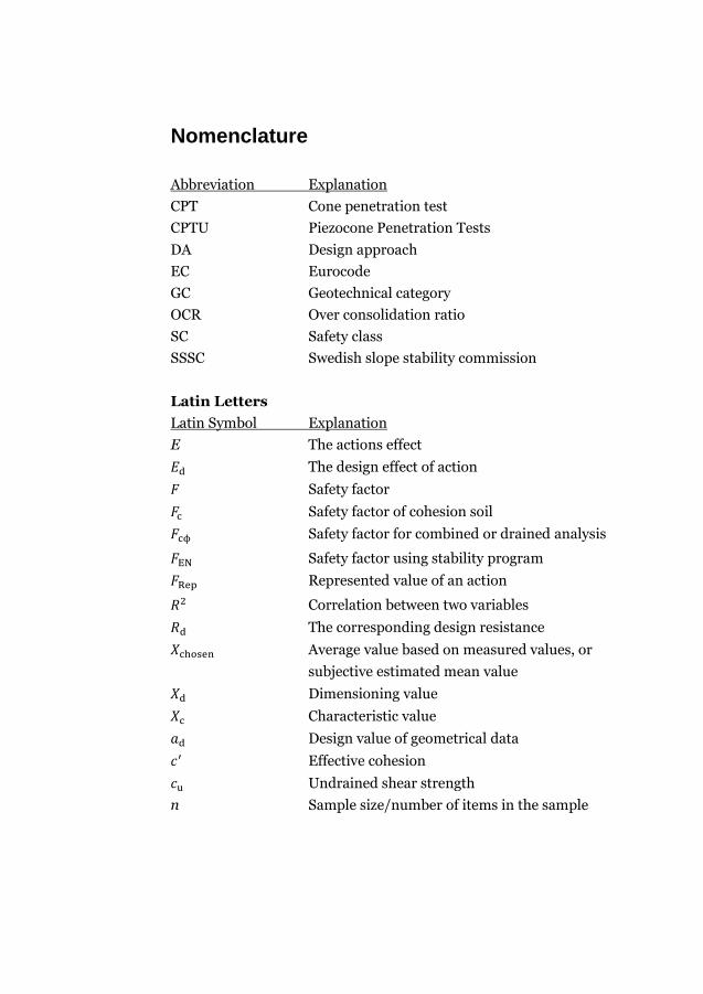
Nomenclature
Abbreviation Explanation
CPT Cone penetration test
CPTU Piezocone Penetration Tests
DA Design approach
EC Eurocode
GC Geotechnical category
OCR Over consolidation ratio
SC Safety class
SSSC Swedish slope stability commission
Latin Letters
Latin Symbol Explanation
E The actions effect
𝐸d The design effect of action
𝐹 Safety factor
𝐹c Safety factor of cohesion soil
𝐹cϕ Safety factor for combined or drained analysis
𝐹EN Safety factor using stability program
𝐹Rep Represented value of an action
𝑅2 Correlation between two variables
𝑅d The corresponding design resistance
𝑋chosen Average value based on measured values, or
subjective estimated mean value
𝑋d Dimensioning value
𝑋c Characteristic value
𝑎d Design value of geometrical data
𝑐′ Effective cohesion
𝑐u Undrained shear strength
n Sample size/number of items in the sample

Greek Letters
Greek Symbol Explanation
𝛾 Unit weight
𝛾d Partial factor
𝛾F Partial factor of action
𝛾M Constant partial coefficient
𝛾m Partial factor of soil parameter
𝛾R Partial factor for bearing capacity
𝜇 Mean value of a scatter
𝜇�̅� Mean value of sampling distribution of the mean
𝜂 Conversion factor
𝜎 Standard deviation
𝜎�̅� Standard deviation of sampling distribution of the
mean
𝜎n Stress
𝜎′ Effective stress
𝜏 Shear strength
𝜏f Shear strength at failure
𝜏fd Drained shear strength at failure
𝜏mob Mobilized shear strength
𝜙 Angle of internal friction
𝜙′ Effective angle of internal friction
ϕc Characteristic value for friction angle
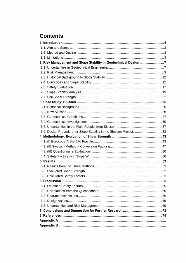
Contents
1.1. Aim and Scope ..................................................................................................... 2
1.2. Method and Outline .............................................................................................. 3
1.3. Limitations ............................................................................................................ 4
2.1. Uncertainties in Geotechnical Engineering ........................................................... 7
2.2. Risk Management ................................................................................................ 9
2.3. Historical Background to Slope Stability ............................................................. 12
2.4. Eurocodes and Slope Stability ............................................................................ 12
2.5. Safety Evaluation ............................................................................................... 17
2.6. Slope Stability Analysis ...................................................................................... 19
2.7. Soil Shear Strength ............................................................................................ 21
3.1. Historical Background ........................................................................................ 25
3.2. New Slussen ...................................................................................................... 26
3.3. Geotechnical Conditions..................................................................................... 27
3.4. Geotechnical Investigations ................................................................................ 30
3.5. Uncertainties in the Field Results from Slussen.................................................. 37
3.6. Design Procedure for Slope Stability in the Slussen Project ............................... 38
4.1. (I) Eurocode 7: the 5 % Fractile .......................................................................... 43
4.2. (II) Swedish Method – Conversion Factor η ........................................................ 47
4.3. (III) Questionnaire Evaluation ............................................................................. 50
4.4. Safety Factors with Slope/W .............................................................................. 50
5.1. Results from the Three Methods ........................................................................ 53
5.2. Evaluated Shear Strength .................................................................................. 62
5.3. Calculated Safety Factors .................................................................................. 63
6.1. Obtained Safety Factors ..................................................................................... 65
6.2. Correlations from the Questionnaire ................................................................... 66
6.3. Characteristic values .......................................................................................... 66
6.4. Design values ..................................................................................................... 69
6.5. Uncertainties and Risk Management .................................................................. 69

INTRODUCTION | 1
Introduction
Site characterization and the subsequent determination of soil strength
parameters constitute a significant part of a slope stability assessment. The
spatial variability that exists in the soil, where measured values located at
different three-dimensional locations, displays values that fluctuate
depending on their position. Spatial variability is a natural and inevitable
characteristic of all soil volumes which entails uncertainties. (Griffiths, et
al., 2009). Geotechnical engineering is always governed by great
uncertainties since the soil properties display large variation and are
challenging to estimate regarding the spatial variability for an entire soil
volume. The task for the geotechnical engineer is to make decisions in the
presence of uncertainties. Investigations can only be carried out in discrete
points and leave most of the soil volume untested. This is one important
difference between geotechnical design and structural design that involves
manufactured materials. In geotechnical design the material properties are
determined rather than specified (Orr & Day, 2002).
One of the most important parameters influencing the assessment of
the stability is the shear resistance that the soil material can mobilize
during shearing. For assessments of slope stability, it is important to
characterize all the different types of uncertainties related to the
geotechnical design properties and calculation models in which the
properties are used and take them into consideration in design. Therefore,
risk management, the work of identification, evaluation and ranking of
risks in a project, are essential.
Before the Eurocode (EC) was introduced, the evaluation of soil
properties based on geotechnical measurements and field tests relied
mainly on the geotechnical engineer’s knowledge, experience and
subjective judgement. With the introduction of the EC, the intent was to
make limit state design with partial factors the new European standard
INTRODUCTION | 2
(CEN, 2004). To evaluate whether a slope is safe enough, safety factors are
normally used. Even though EC dose not advocate a global safety factor for
practical design it is possible to use on order to compare the influence from
a single variable, since it is then possible to study its influence individually.
Otherwise different partial factors will be included for friction soil and clay,
partial factor on the load and load coefficient for the safety class. For these
not to influence the result, the global safety factor is used, which is common
in numerical models (Potts & Zdravovic, 2012). The required safety factor
Fc for slopes in the highest safety class, safety class 3, and undrained
conditions is 1.65 (Swedish Transport Administration, 2011).
The situation is that today there exists no standardized method that is
used for determination of soil parameters. Different countries have their
own approach for estimation of soil parameters, for example the EC 7 and
Bayesian statistics, while Sweden follows the “Implementation
Commission for European Standards in Geotechnology” (IEG) report
complementing EC. Every country has its own approach on how to handle
uncertainties and how to take them into consideration. Many methods are
also still built upon the assessment of the engineer’s knowledge and
experience. This leads to several possible outcomes of soil parameters
which will affect the stability assessment. It is necessary to be on the safe
side, but not “too safe” from an economical perspective.
1.1. Aim and Scope
The aim of this thesis is to examine how different methods affect the
evaluation of the characteristic value of the undrained shear strength 𝑐u in
clay for heterogeneous soil. This is essential from a slope stability
perspective since the parameter has a great influence on the calculated
stability and hence the safety. The three used methods are:
(I) The 5 % fractile of the mean value according to Eurocode 7
(II) The Swedish method with the η-factor according to the IEG-
report 6:2008 slopes and embankments.

INTRODUCTION | 3
(III) A questionnaire where geotechnical engineers were asked to
“estimate a cautiously assumed mean value”. Also in
accordance with Eurocode 7, Clause 2.4.5.2(2).
Possible correlations that will influence for the subjective judgement of the
geotechnical engineer’s will be studied based on the questionnaire. Also a
closer look how risk management is incorporated into the slope stability
work order.
1.2. Method and Outline
To investigate this problem, to determine the characteristic value of 𝑐u of
clay for slopes located at three quaysides in Slussen in Stockholm. The site
data is based on the same CPT results obtained from the three areas. The
methods of investigation.
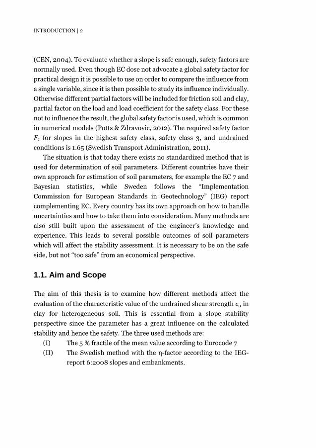
The thesis work was carried out in three main stages, see Figure 1. First
stage is a literature review, followed by evaluation of the characteristic
value of the shear strength with the three different methods (I), (II) and
(III). This is followed by calculations using the software program Slope/W
to determine the safety factor to see the influence of the evaluated shear
strength on the safety. Lastly interpretation of the results, discussion and
conclusion.
The literature review is presented in chapter 2 and 3. In chapter 2 a
closer look are taken to at risk management and uncertainties in
geotechnical engineering and slope stability with a historical background,
EC and the shear strength parameter. In chapter 3, Slussen, an area in the
centre of Stockholm and the design procedure for slope stability analysis is
discussed together with risk management in the project.
The second stage was to evaluate 𝑐u for the clay layer by using the three
different methods (I), (II) and (III). Together with calculations using
Slope/W to evaluate how the soil properties at the area of Slussen will
influence the global stability and determine a safety factor for each section.
The last stage was to interpret the results, discussion and conclusion
followed by suggestions for further research.
INTRODUCTION | 4
Figure 1 - Outline of thesis work
1.3. Limitations
The location of the investigation was Slussen, and three slopes’ cross-
sections were chosen for applying the three methods in this thesis work,
one is located at Guldfjärdsplan, one at Munkbron and the last one at
Skeppsbrokajen. The investigated soil parameter was limited to the direct
undrained shear strength in the clay layer for each section, i.e. strength
anisotropy is not taken into consideration. The analysed material came
Sta
ge
2
Sta
ge
3
Chapter 2: Slope stability in geotechnical design - Uncertainties and risk management
- Historical background
- Eurocode 7
- Slopes Stability analysis
- Soil shear strength
Chapter 3: Case study - Slussen
- Design procedure
Chapter 4: Evaluation shear strength/calculations SF - (I) Eurocode 7 – 5% fractile
- (II) Swedish method – η factor
- (III) Questionnaire evaluation
- Safety factor with Slope/W
Chapter 5: Results
Chapter 6: Discussion
Chapter 7: Conclusions and future
researches
Sta
ge
1

INTRODUCTION | 5
from CPT tests and it is evaluated with CONRAD version 3.0 and presented
in “CONRAD evaluation” (Exploateringskontoret, 2016).
In this thesis work, the term “clay layer” refers to a cross-section/layer
in the soil strata that has a higher clay or organic content than the rest. The
characterisation for the area is that the soil is non-homogenous. Therefore,
it is not a homogenous clay layer, but rather a mix of fill and organic
content/clay/mud (see chapter 3.3 page 27 for a full explanation of the soil
strata at Slussen). Furthermore, to simplify the study, a value for 𝑐u with
no regard to spatial variability in the clay layer is determined. The
assumption was that the parameter is not varying with the depth in the soil
strata or has any spatial variability horizontally that is utilised but serves
to idealize the field conditions.


LITERATURE STUDY | 7
Risk Management and Slope Stability in
Geotechnical Design
2.1. Uncertainties in Geotechnical Engineering
Geotechnical engineering is always governed by great uncertainties since
the soil properties are not clear and hard to estimate for an entire soil
volume (Fenton & Griffiths, 2008). Investigations can only be performed
in discrete points and leave the majority of the soil volume untested.
Uncertainties also arise in measurement errors, in the measuring
equipment and inherent in the used method (Prästings, 2016). For safety
calculations of slope stability, it is important to recognise all different types
of uncertainties related to the geotechnical design properties and
calculation models in which the properties are used (Fenton & Griffiths,
2008). To evaluate the reliability of the safety factor it is necessary to
understand all the inherent uncertainties that exist.
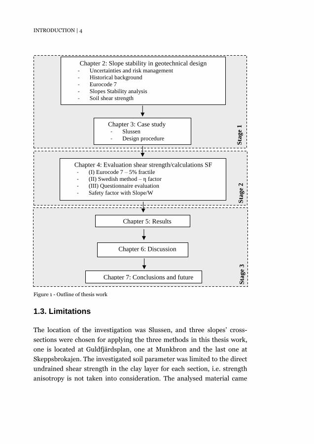
Uncertainties can be divided into two groups, aleatory and epistemic,
see Figure 2. Aleatoric uncertainties or statistical uncertainties are true
random behaviour, it relates to natural phenomena and inherent or natural
uncertainty and the results differ each time the experiment is performed.
Aleatoric uncertainties can never be reduced because they are related to
inherent spatial variability in the soil. It is crucial to evaluate whether the
obtained result is dominated by true random errors or not (Apel, et al.,
2004).
An epistemic uncertainty or systematic uncertainty is when there is a
lack of knowledge about a property. The epistemic uncertainties can be
reduced with increased knowledge. This can be obtained in geotechnical
engineering by doing more field- and probing tests and analysis, improving
the quality in the measurement procedure or improving the accuracy of the
calculation models.
LITERATURE STUDY | 8
Figure 2 – Geotechnical uncertainties and where they arise from
However, there are always some uncertainties about how well the
parameters have been estimated that can never be eliminated. The more
that is known about the soil, the lower is the epistemic uncertainty and
more reliable results can be received. The epistemic uncertainties can
therefore be said to relate to our ability to understand, measure and
describe the system under study (Sun, et al., 2012).
According to Phoon and Kulhaway (1999), it is important to understand
where uncertainties arise and how to prevent them. The three main sources
where uncertainties originate from are 1) inherent soil variability; 2)
measurement errors and 3) transformation uncertainties. Inherent soil
variability (1) comes from the geological process in which the soil has been
formed. The uncertainties are related to the varying nature of the soil, the
parameters will fluctuate both horizontally and vertically (Fenton &
Griffiths, 2008). The uncertainties can be reduced by performing more
geotechnical investigations and monitoring every location in the soil. The
second source, measurement errors (2), are inherent from equipment,
operator or random testing effects. Measurement errors arise from
equipment-, procedure- and operator effects and they are systematic.
There also exist random measurement errors, and they are hard to separate
from inherent spatial variability, since both are random variations along
the trend. The last category, transformation uncertainties (3), and they
relate to the process when in-situ or laboratory results are transformed to
an appropriate design property to accommodate the requirements. The
transformation is often based on models obtained by empirical data fitting
Epistemic uncertainties
Geotechnical uncertainties
Aleatory uncertainties
Data scatter
Inherent/spatial variability Measurement errors
Statistical errors Transformation errors
LITERATURE STUDY | 9
or by theoretical relationships and will always contain some degree of
uncertainty. Transformation uncertainty would still be present even for
theoretical relationships because of idealizations and simplifications in the
theory.
The main question is not whether to deal with uncertainties or not, but
rather be aware that they exist and understand how to consider the
uncertainties and take them into account.
2.2. Risk Management
The report from Swedish Geotechnical Society about “Risk management in
geotechnical engineering projects – requirements: methodology” (SGF,
2017; Spross et al, 2017) addresses the topic about geotechnical risk
management. Risk management includes not only the structural design
and its safety, but also project economy, environmental impact, work
environment and third-party disturbance. Repercussions that bad risk
management can lead to are human injuries, unexpected costs and delays.
Geotechnical risk management is about a general procedure for how to
manage uncertainties that may threaten defined goals in geotechnical
engineering projects. SGF applies in their report the definition by ISO
31000:2009 where risk is defined as “effect of uncertainties on objects”,
but with minor adjustment, only negative effects are considered. ISO
defines risk management as “coordinated activities to direct and control
organization with regard to risk” (ISO, 2009). Here “uncertainties” stand
for how not fully known geological conditions affects our objective to build
a structure with sufficient quality. And “objects” stand for how to build a
structure that satisfies the owner’s requirements and society’s safety
requirements, with minimized environmental impact.
LITERATURE STUDY | 10
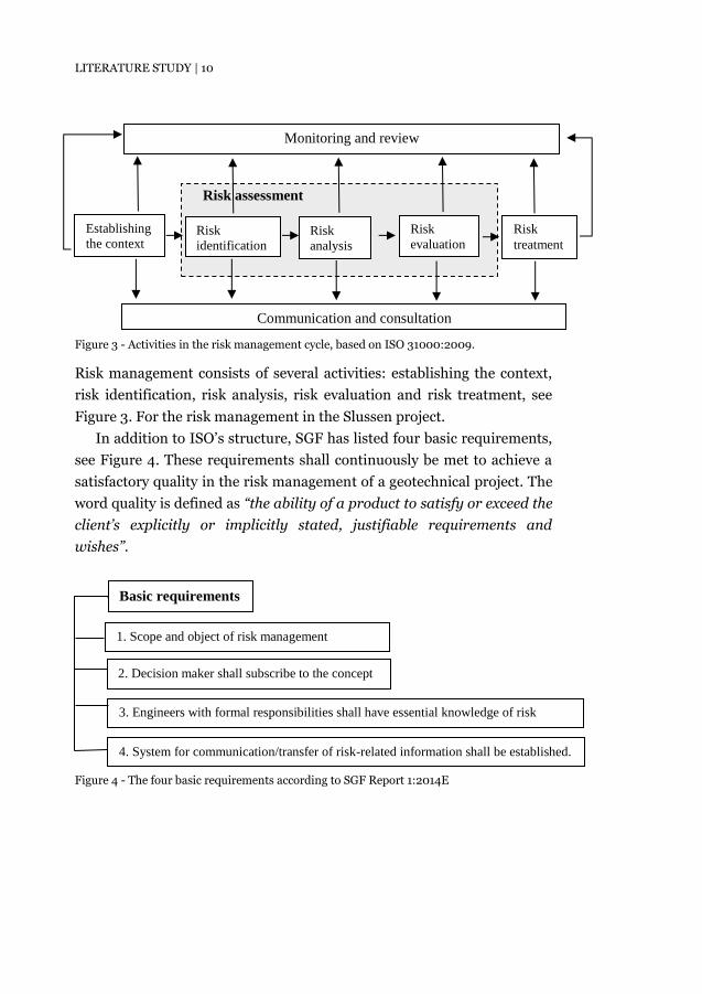
Figure 3 - Activities in the risk management cycle, based on ISO 31000:2009.
Risk management consists of several activities: establishing the context,
risk identification, risk analysis, risk evaluation and risk treatment, see
Figure 3. For the risk management in the Slussen project.
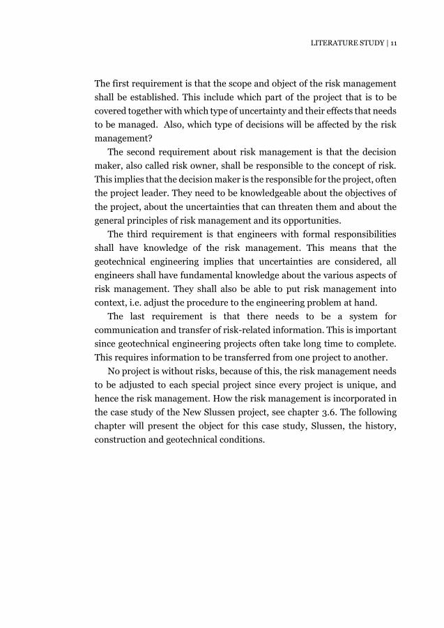
In addition to ISO’s structure, SGF has listed four basic requirements,
see Figure 4. These requirements shall continuously be met to achieve a
satisfactory quality in the risk management of a geotechnical project. The
word quality is defined as “the ability of a product to satisfy or exceed the
client’s explicitly or implicitly stated, justifiable requirements and
wishes”.
Figure 4 - The four basic requirements according to SGF Report 1:2014E
Establishing
the context Risk
evaluation
Risk
treatment Risk
identification Risk
analysis
Risk assessment
Communication and consultation
Monitoring and review
Basic requirements
1. Scope and object of risk management
2. Decision maker shall subscribe to the concept
of risk
3. Engineers with formal responsibilities shall have essential knowledge of risk
management
4. System for communication/transfer of risk-related information shall be established.
LITERATURE STUDY | 11
The first requirement is that the scope and object of the risk management
shall be established. This include which part of the project that is to be
covered together with which type of uncertainty and their effects that needs
to be managed. Also, which type of decisions will be affected by the risk
management?
The second requirement about risk management is that the decision
maker, also called risk owner, shall be responsible to the concept of risk.
This implies that the decision maker is the responsible for the project, often
the project leader. They need to be knowledgeable about the objectives of
the project, about the uncertainties that can threaten them and about the
general principles of risk management and its opportunities.
The third requirement is that engineers with formal responsibilities
shall have knowledge of the risk management. This means that the
geotechnical engineering implies that uncertainties are considered, all
engineers shall have fundamental knowledge about the various aspects of
risk management. They shall also be able to put risk management into
context, i.e. adjust the procedure to the engineering problem at hand.
The last requirement is that there needs to be a system for
communication and transfer of risk-related information. This is important
since geotechnical engineering projects often take long time to complete.
This requires information to be transferred from one project to another.
No project is without risks, because of this, the risk management needs
to be adjusted to each special project since every project is unique, and
hence the risk management. How the risk management is incorporated in
the case study of the New Slussen project, see chapter 3.6. The following
chapter will present the object for this case study, Slussen, the history,
construction and geotechnical conditions.
LITERATURE STUDY | 12
2.3. Historical Background to Slope Stability
Many problems regarding slope stability are associated with uncertainties,
the design and construction of unbraced cuts, e.g. highways, railways and
canals. The necessity to excavate deep cuts did not arise until early in the
19th century, when the first railways were built. Since then, the cuts with
increasing depth and length have been excavated (Terzaghi & Peck, 1948).
According to the “Swedish Slope stability commission” (SSSC, 1995), in
Sweden, slopes with propensity for landslides are usually inclined areas of
clay, (slope > 1:10) with the possibility of high pore pressures and shear
stresses in the clay, for example at watercourses at valleys, with elongated
inclination, near topographical located higher ground or loaded ground
with clay adjacent to watercourses. Especially probable to fail are slopes
along watercourses, where erosion can deteriorate the down-slope
counterweight (Morgenstern & Price, 1965).
The stability of slopes has been calculated by hand since the 1920s and
with different methods like Janbu’s, Bishop, Morgenstern-Prince, Spencer
etc called limit equilibrium methods (Abramson, et al., 2002). Since then,
computer programs for slope stability assessment have increasingly been
applied in design, but the “classical” calculation methods remain the same.
Among the most used program in the world today is Slope/W. The program
is based on the limit equilibrium-analysis for calculations regarding slope
stability (Geo-Slope, 2004).
2.4. Eurocodes and Slope Stability
2.4.1. The Eurocode
The EC are the European standards, specifying how structural design
should be conducted within the European Union. The EC were conceived
by the European Commission in the 1970s as a group of coherent European
standards for the structural and geotechnical design of buildings and civil
engineering works (CEN, 2002). EC 7 also known as EN 1997, describes
how to design geotechnical structures. It was published in two parts:
LITERATURE STUDY | 13
“general rules” (EN 1997-1) and “ground investigation and testing” (EN
1997-2) (Orr & Farrell, 2012).
EC 7 has been the primary geotechnical design code in Europe since
2010. It has replaced the national design codes, while allowing for national
annexes to be introduced, which can account for local practice. Among the
biggest changes in the design practice introduced by the EC were the partial
factors on soil strength, resistance and applied loads. They were innovative
since EC requires uncertainties in the design procedure to be taken into
consideration more explicitly and in a constant approach. But EC is also
conventional in that it provides little guidance on how this should be
achieved, especially with respect to the determination of so-called
characteristic soil property values used in the design (Arnold, et al., 2013).
2.4.2. Design Approaches in Eurocode
Three Design Approaches are available in EC: DA1, DA2 and DA3, see
Table 1, and each country has essentially adopted one of them (Potts &
Zdravovic, 2012). In Sweden, DA3 is applied for slopes and embankments,
(EKS, 2013).
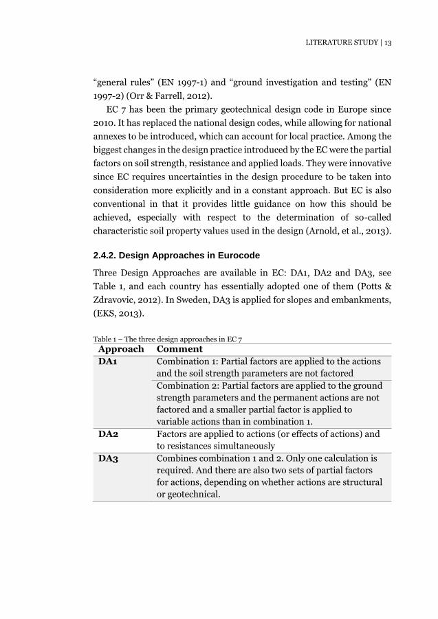
Table 1 – The three design approaches in EC 7
Approach Comment
DA1 Combination 1: Partial factors are applied to the actions
and the soil strength parameters are not factored
Combination 2: Partial factors are applied to the ground
strength parameters and the permanent actions are not
factored and a smaller partial factor is applied to
variable actions than in combination 1.
DA2 Factors are applied to actions (or effects of actions) and
to resistances simultaneously
DA3 Combines combination 1 and 2. Only one calculation is
required. And there are also two sets of partial factors
for actions, depending on whether actions are structural
or geotechnical.
LITERATURE STUDY | 14
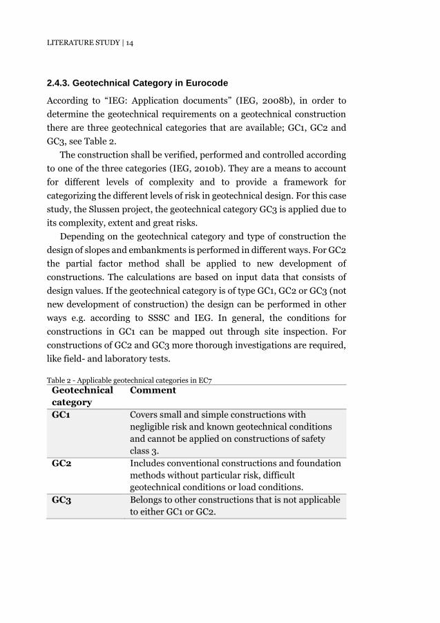
2.4.3. Geotechnical Category in Eurocode
According to “IEG: Application documents” (IEG, 2008b), in order to
determine the geotechnical requirements on a geotechnical construction
there are three geotechnical categories that are available; GC1, GC2 and
GC3, see Table 2.
The construction shall be verified, performed and controlled according
to one of the three categories (IEG, 2010b). They are a means to account
for different levels of complexity and to provide a framework for
categorizing the different levels of risk in geotechnical design. For this case
study, the Slussen project, the geotechnical category GC3 is applied due to
its complexity, extent and great risks.
Depending on the geotechnical category and type of construction the
design of slopes and embankments is performed in different ways. For GC2
the partial factor method shall be applied to new development of
constructions. The calculations are based on input data that consists of
design values. If the geotechnical category is of type GC1, GC2 or GC3 (not
new development of construction) the design can be performed in other
ways e.g. according to SSSC and IEG. In general, the conditions for
constructions in GC1 can be mapped out through site inspection. For
constructions of GC2 and GC3 more thorough investigations are required,
like field- and laboratory tests.
Table 2 - Applicable geotechnical categories in EC7
Geotechnical
category
Comment
GC1 Covers small and simple constructions with
negligible risk and known geotechnical conditions
and cannot be applied on constructions of safety
class 3.
GC2 Includes conventional constructions and foundation
methods without particular risk, difficult
geotechnical conditions or load conditions.
GC3 Belongs to other constructions that is not applicable
to either GC1 or GC2.

LITERATURE STUDY | 15
2.4.4. Safety Class in Eurocode
Safety classes according to SS-EN 1997 are divided into three categories
depending on consequences of an eventual failure with corresponding
partial factors. For design with the partial coefficient method the loads are
modified by multiplication with the corresponding partial factor, (𝛾𝑑)
regarding the safety class. The determination of the safety class is
performed according to EC 7 and is also regulated with BFS 2009:16 and
VVFS 2009:19. The safety class is depending on the type of construction,
Table 3.
Table 3 - Safety classes with corresponding partial factor in EC7
Safety class Description Partial factor [-]
SC1 (Low) Small risk of serious damage to people 𝛾𝑑 = 0.83
SC2 (Normal) Some risk for serious damage to people 𝛾𝑑 = 0.91
SC3 (High) Great risk for serious damage to people 𝛾𝑑 = 1.00
2.4.5. The 5 % Fractile According to Eurocode
EC 7 defines the characteristic value as a cautious estimate of the value
affecting the limit state, considering the following factors, paragraph
“2.4.5.2 (4) (CEN, 2004)
Geological and other background information, such as data from
previous projects
The variability of the measured property values and other relevant
information
The extent of the field and laboratory investigation
The type and number of samples
The extent of the zone of ground governing the behaviour of the
geotechnical structure at the limit state being considered
The ability of the geotechnical structure to transfer loads from
weak to strong zones in the ground”
In EC 7 it is stated that “if statistical methods are used, the
characteristic value should be derived such that the calculated probability
of a worse value governing the occurrence of the limit state under
consideration is not greater than 5%” (Clause 2.4.5.2 (11)) (CEN, 2004).
LITERATURE STUDY | 16
This implies a confidence level of 95%. Statistic methods can be used to
determine the characteristic values of the geotechnical parameters. The
characteristic value is selected such that there is only a small probability
that the value governing the limit state in the ground will be less favourable
than the characteristic value. A requirement for using statistical methods
is that there exist a sufficiently large number of test results. In EC 7, it is
recommended that the calculated probability of the minimum value
governing the occurrence of the limit state considered should not be
greater than 5 % (Frank, et al., 2005). The 5 % fractile can be applied on
either the entire population, which then considers local failure, a system of
weakest link. Or 5 % fractile can be applied to the mean value, this is more
realistic, the sliding surface is then seen as an averaging system.
2.4.6. Swedish National Annex to Eurocode
The Swedish national application document is written by IEG. IEG is a
non-governmental association that operates under academy for the Royal
Engineering Sciences. IEG is responsible for initiating, coordinating,
implementing and reporting work required to implement European
standards in the field of Geotechnical Engineering in Sweden.
The Swedish application documents TRVFS, EKS and “Application
document – the basics of Eurocode 7” (IEG, 2010b), are used together with
EC 7 for geotechnical engineering. Special for the annex, IEG-report
6:2008 slopes and embankments, is the conversion factor 𝜂, which implies
a possible adjustment of the fixed partial factor. The η-factor considers the
soil as well as the extent and quality of soil investigations. Furthermore, η
also considers the geometry and design of the geotechnical construction as
well as the mechanical system.
The Swedish method, using the national application document to EC 7
considers the same uncertainties and factors listed in EC 7 clause 2.4.5.2
(4), the difference is that they are now regarded in the evaluation of η. Also
the η factor is included to adjust for the level of uncertainties in the
material property. This is discussed and evaluated in Prästings, et al,
(2017).

LITERATURE STUDY | 17
2.5. Safety Evaluation
The magnitude of the acceptable safety factor should reflect both
probability and consequence of failure (Arnold, et al., 2013). Design
implies finding the right balance between uncertainties, consequences and
acceptable risks. The necessary calculated safety factor for the slope
stability depends on several factors e.g. soil type, approach to the problem
and consequences of an eventual failure (SSSC, 1995).
The concept of safety factors in design of geotechnical structures has
traditionally been developed within the framework of classical soil
mechanics. With the classical analysis, the calculations involve simple limit
equilibrium or limit analysis approach. The basic principle of the classical
approach to slope stability analysis was to search for the minimum factor
of safety with respect to shear failure (Janbu, 2001). The safety factor, F is
defined according to the classical analysis as the relationship between,
shear strength at failure 𝜏f, and the mobilized shear strength, 𝜏mob, along a
sliding surface
𝐹 =𝜏𝑓
𝜏mob
(1)
The expression is essentially used by all slope stability analysis methods,
such as limit equilibrium methods, finite element methods and limit
analysis approaches (SSSC, 1995).
In the limit-state method, verification of the ultimate limit state of
strength is expressed in EC 7 and SS-EN 1997 by
𝐸d ≤ 𝑅d (2)
𝐸d = 𝐸{𝛾F𝐹Rep; 𝑋𝑐/𝛾m ; 𝑎d} (3)
𝑅d = 𝑅{𝛾F𝐹Rep; 𝑋𝑐/𝛾m ; 𝑎d} or (4)
𝑅d = 𝑅{𝛾F𝐹Rep; 𝑋𝑐 ; 𝑎d}/𝛾R (5)
LITERATURE STUDY | 18
Partial factors on actions may be applied to the actions themselves FRep or
to their effects E. 𝐸d stands for the design effect of action, 𝑅d the
corresponding design resistance, 𝑋c the characteristic value and 𝛾m a
partial factor. Although this method considers different loading conditions
by using suitable combinations of design values, it is still based on direct
comparison of the available shear strength with the mobilized stresses.
These expressions apply to the following ultimate limit states:
GEO: “Failure or excessive deformation of the ground, in which
the strength of soil or rock is significant in providing resistance”
STR: “Internal failure or excessive deformation of the structure
or structural elements in which the strength of structural
materials is significant in providing resistance”
As mentioned in the introduction, even though EC does not advocate a
global safety factor for practical design it is possible to use in order to
compare the influence from a single variable, since it is then possible to
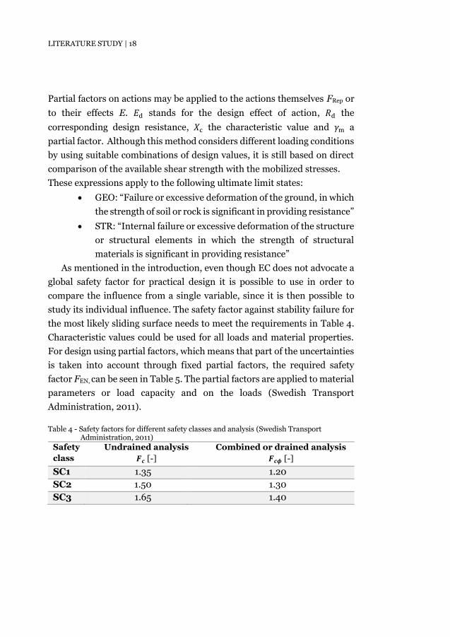
study its individual influence. The safety factor against stability failure for
the most likely sliding surface needs to meet the requirements in Table 4.
Characteristic values could be used for all loads and material properties.
For design using partial factors, which means that part of the uncertainties
is taken into account through fixed partial factors, the required safety
factor FEN, can be seen in Table 5. The partial factors are applied to material
parameters or load capacity and on the loads (Swedish Transport
Administration, 2011).
Table 4 - Safety factors for different safety classes and analysis (Swedish Transport Administration, 2011)
Safety
class
Undrained analysis
𝑭𝒄 [-]
Combined or drained analysis
𝑭𝒄𝝓 [-]
SC1 1.35 1.20
SC2 1.50 1.30
SC3 1.65 1.40

LITERATURE STUDY | 19
Table 5 – FEN for calculations with stability programs based on the global safety (Swedish Transport Administration, 2011)
Safety class FEN [-]
SC1 0.90
SC2 1.00
SC3 1.10
2.6. Slope Stability Analysis
The main purpose of performing a slope stability analysis is to understand
and determine the safety of the slope against sliding failure. The sensitivity
to different triggering mechanisms and to evaluate the stability regarding
long-term and short-term conditions is often considered. Slope stability
assessment can be used to investigate potential failure mechanisms and
test different support and stabilization options. It can also be applied to
design optimal excavated slopes in terms of safety, reliability and
economics (Abramson, et al., 2002).
Slope failures involves a large variety of processes and factors causing
the failure, consequently it exists an unlimited possibility of slides. It is
difficult to apply a general design procedure which can be functional for all
the different scenarios that can arise regarding slope stability. Normally a
reasonable scope is considered and then the investigation gradually
increases until the slope is considered safe enough based on the calculated
safety factor. (SSSC, 1995)
2.6.1. General Limit Equilibrium Formulation
Limit equilibrium formulations based on the method of slices are applied
more to the stability analysis of structures, for example tie back walls, nail
or fabric reinforced slopes, sliding stability of structures subjected to high
horizontal loading arising. Many methods of slices have been developed
(Janbu, 2001). There exist two significant differences between all the
methods:
what equations of static equilibrium are included and satisfied
what interslice forces are included and what is the assumed
relationship between the interslice shear and normal forces
LITERATURE STUDY | 20
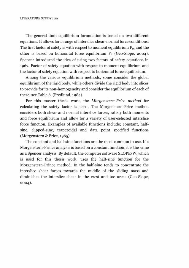
The general limit equilibrium formulation is based on two different
equations. It allows for a range of interslice shear-normal force conditions.
The first factor of safety is with respect to moment equilibrium F𝑚 and the
other is based on horizontal force equilibrium F𝑓 (Geo-Slope, 2004).
Spencer introduced the idea of using two factors of safety equations in
1967. Factor of safety equation with respect to moment equilibrium and
the factor of safety equation with respect to horizontal force equilibrium.
Among the various equilibrium methods, some consider the global
equilibrium of the rigid body, while others divide the rigid body into slices
to provide for its non-homogeneity and consider the equilibrium of each of
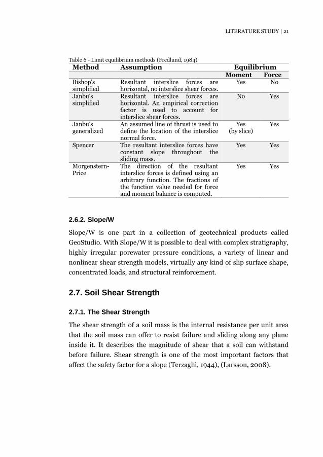
these, see Table 6 (Fredlund, 1984).
For this master thesis work, the Morgenstern-Price method for
calculating the safety factor is used. The Morgenstern-Price method
considers both shear and normal interslice forces, satisfy both moments
and force equilibrium and allow for a variety of user-selected interslice
force function. Examples of available functions include; constant, half-
sine, clipped-sine, trapezoidal and data point specified functions
(Morgenstern & Price, 1965).
The constant and half-sine functions are the most common to use. If a
Morgenstern-Prince analysis is based on a constant function, it is the same
as a Spencer analysis. By default, the computer software SLOPE/W, which
is used for this thesis work, uses the half-sine function for the
Morgenstern-Prince method. In the half-sine tends to concentrate the
interslice shear forces towards the middle of the sliding mass and
diminishes the interslice shear in the crest and toe areas (Geo-Slope,
2004).
LITERATURE STUDY | 21
Table 6 - Limit equilibrium methods (Fredlund, 1984)
Method Assumption Equilibrium Moment Force
Bishop's simplified
Resultant interslice forces are horizontal, no interslice shear forces.
Yes No
Janbu's simplified
Resultant interslice forces are horizontal. An empirical correction factor is used to account for interslice shear forces.
No Yes
Janbu's generalized
An assumed line of thrust is used to define the location of the interslice normal force.
Yes (by slice)
Yes
Spencer The resultant interslice forces have constant slope throughout the sliding mass.
Yes Yes
Morgenstern-Price
The direction of the resultant interslice forces is defined using an arbitrary function. The fractions of the function value needed for force and moment balance is computed.
Yes Yes
2.6.2. Slope/W
Slope/W is one part in a collection of geotechnical products called
GeoStudio. With Slope/W it is possible to deal with complex stratigraphy,
highly irregular porewater pressure conditions, a variety of linear and
nonlinear shear strength models, virtually any kind of slip surface shape,
concentrated loads, and structural reinforcement.
2.7. Soil Shear Strength
2.7.1. The Shear Strength
The shear strength of a soil mass is the internal resistance per unit area
that the soil mass can offer to resist failure and sliding along any plane
inside it. It describes the magnitude of shear that a soil can withstand
before failure. Shear strength is one of the most important factors that
affect the safety factor for a slope (Terzaghi, 1944), (Larsson, 2008).

LITERATURE STUDY | 22
Figure 5 - Graphical representation of Coulomb shear strength equation
Soils generally fail in shear and at failure, shear stress along the failure
surface, 𝜏, (mobilized shear resistance) reaches the shear strength 𝜏f. The
shear strength is the maximum shear stress the soil can resist without
failure. Shear strength is normally divided into drained or undrained
analysis, mainly depending on permeability in the soil mass and the rate of
loading.
The most common way to describe the shear strength is by Coulomb’s
equation. This equation represents a straight line in a shear stress versus
normal stress plot, see Figure 5. The intercept on the shear strength axis is
the cohesion, c, and the slope of the line is the angle of internal friction, 𝜙
(Terzaghi, 1944).
2.7.2. Drained Analysis
The drained shear strength is the shear strength under drained conditions.
This occurs when pore fluid pressures, generated during shearing the soil,
can dissipate during shearing. It also applies where no pore water exists in
the soil, the soil is dry, and hence pore fluid pressures are negligible.
By using Mohr-Coulomb failure criterion, Figure 6, in combination with
the principle of effective stress (Terzaghi, 1944), it can be approximated
empirically with
𝜏 = 𝜏fd = 𝑐′ + 𝜎′ ∙ 𝑡𝑎𝑛𝜙′ (6)
𝜙
𝑐
𝜎𝑛
𝜏

LITERATURE STUDY | 23
Figure 6 - Mohr-Coulomb failure criterion, drained conditions
2.7.3. Undrained Analysis
In undrained conditions, where 𝜙 = 0 by definition, the failure envelop
appears, as shown in Figure 7, because ∆𝜎′1 = ∆𝜎3′ = ∆𝑢. The soil strength
is described by the cohesion, c. The undrained shear strength
𝜏f = 𝑐u (7)
depends on the overconsolidation, the orientation of stresses, stress path,
mode of failure, soil anisotropy, rate of sheering and volume of the soil
material (Larsson, et al., 2007). The overconsolidation ratio, OCR, is the
ratio of the maximum past effective mean stress to the current applied
stress (Terzaghi, 1944). For clay, OCR is a key property required to
characterize its mechanical behaviour (Schnaid, 2009).
The undrained shear strength is not expressed as a single value that is
a representative for the whole soil mass, as it is not a constant. It varies
with the stress direction in the soil and it can be classified accordingly. The
undrained shear strength is normally divided into three cases, active-,
direct-, and passive shearing, see Figure 8. The active shear stress occurs
when the major stress is vertical, the passive when the shear stress is
horizontal and direct at direct shear in a horizontal sliding surface
(Larsson, et al., 2007). The relation between the soils undrained shear
𝜙
𝑐
𝜎𝑛
𝜏
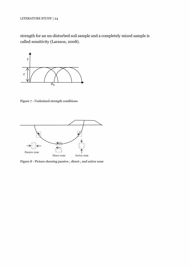
LITERATURE STUDY | 24
strength for an un-disturbed soil sample and a completely mixed sample is
called sensitivity (Larsson, 2008).
Figure 7 - Undrained strength conditions
Figure 8 - Picture showing passive-, direct-, and active zone
𝑐
𝜎𝑛
𝜏
Passive zone
Direct zone Active zone

CASE STUDY | 25
Case Study: Slussen
As mentioned in the introduction, the focus area for this thesis work is
Slussen, located in the centre of Stockholm. Three areas have been chosen:
Guldfjärdsplan, Munkbron and Skeppsbrokajen. The soil strata at Slussen
are very complicated which makes it difficult to categorize and estimate the
soil parameters since the soil is highly heterogeneous. It is also a large
project with high complexity which requires substantial risk management.
This makes it a good object to study in this thesis work.
3.1. Historical Background
Slussen is an area in Stockholm located at the centre of the capital on the
Söderström inlet, connecting Södermalm and Gamla Stan. This is a historic
area where many bridge and lock structures have been built. The first lock,
Queen Kristinas lock (named after the Swedish queen Kristina) was opened
in 1642. In 1755 the second lock was finished (Polhems lock) and in 1850
the third lock (Nils Ericson’s) was completed.
Slussen was planned and constructed to solve the traffic problems of its
time. In 1920, Stockholm had around 420 000 residents. The bridges at
Slussen were still the only route connecting North and South Stockholm.
The forth lock, Karl Johan lock, was inaugurated in 1935. Now it was no
longer necessary to open the bridges at Slussen, since Hammarby lock
could be opened for larger vessels. The purpose of the new structure was to
alleviate the situation for the increasing number of car users.
Figure 9 – The construction of Slussen that was finished in 1935 (Stockholms Stad, 2014)
CASE STUDY | 26
The Slussen viaduct, in its simplest form was inaugurated by the king
Gustaf V in 1933. It was the end station for the underground tram but in
1950 it became the terminal of the first metro line and was rebuilt again in
1957 when the line to Hötorget was opened. The Slussen metro station has
become a hub of public transport, serving the red and green subway lines,
with a connecting bus terminal and Saltsjöbanan commuter rail station
serving the eastern parts of Stockholm. Slussen has approximately
138 800 arriving passengers per day and is therefore Stockholm's second
largest public transport point after the Central Station (AB Storstockholms
Lokaltrafik, 2016).
The structure existing today, which is to be re-built, was finished in
1935. It is a concrete structure with its trademark; the cloverleaf
interchange, see Figure 9. The piling for the construction has proved
insufficient for its purpose, which has created significant settlements of up
to 25 centimetres (Lorentzi, et al., 2005).
3.2. New Slussen
Today, Slussen is in a deprived condition due to the poor quality of the
concrete used in the 1930s that has weathered in many places mainly
because it is not salt-resistant. After many years of planning, it is now time
to rebuild Slussen, so it can last for the future. The foundation for the new
structure is one of the most complicated and comprehensive foundations
in Sweden and requires substantial geotechnical investigations
(Stockholms Stad, 2017).
The new Slussen project is a collaboration concept by traffic- and urban
construction offices. The architectural design is completed by Foster and
Partners in collaboration with Berg Arkitektkontor. The concept for the
project is to create a modern city area. The new Slussen will provide new
public spaces, a more accessible quayside, pedestrian and cycle routes
while transforming the existing infrastructure to minimise the threat of
flooding and creating a 21st century transport interchange. The new
Slussen is expected to be finished in 2025 (Foster and Partners, 2018).

CASE STUDY | 27
3.3. Geotechnical Conditions
3.3.1. The Nature of Slussen
The nature of the area originates from the Söderström-fault zone in the
bedrock that extend from Söder Mälarstrand to Stadsgårdskajen in a west-
north direction. The fault contributes to very sharp mountain cliffs and
deep mountain ranges in the area. The highest point located at the block
Urvädersklippan at level +30 m and the lowest in the northern part of
Guldfjärdsplan at -74 m. The Söderström-fault zone crosses the wide
Stockholm esker that runs across the centre of Slussen in north-south
direction, from Södermalm onward over Stadsholmen and cuts of the
connection between Saltsjön and Mälaren (Exploateringskontoret, 2011).
Figure 10 - Slussen today with the shore line from the 1200, reproduced with permission from
(Blom)
CASE STUDY | 28
Earlier experience from previous foundation works at Slussen has shown
that the geotechnical conditions in the area are very unfavourable. Mud
and clay layers are in great extent covered by man-made deposits that have
been dumped during hundreds of years, and the layers are highly
heterogeneous (Stockholms Stad, ). Since the 13th century, successively
filled areas and the isostasy of more than 3 meter have made the shoreline
rise substantially and the area has undergone big topographical changes,
see Figure 10 for the old shoreline (Exploateringskontoret, 2011).
The esker has a complicated geological structure, both externally and
internally. The surface consists of sand, gravel, clay and glaciofluvial
deposits. The internal part consists of a high proportion of rounded blocks
and boulders, around which gravel and sand are stored with a very
changing composition. The esker lies directly on the bedrock (Stockholms
Stad, ).
Post-glacial clay, organic clay and mud largely cover the areas
previously made up of seabed. Fine-grained soils with organic content are
common in Sweden. Even the glacial clays often contain some amount of
organic material. In many areas the content is so high that the soils are
classified as organic clay or gyttja (Larsson, 1990). The organic clay in
consists of clay deposits from the Mälaren region, see Figure 11. By
comparing the old shoreline with the extent of the mud and clay, it can be
noticed that the area with the clay is located where the old sea line was
positioned. In relation with the extensions that have taken place
throughout the ages, sediment layers have been compacted due to the fill.
The fill has been placed in stages which means that the fill is mixed with
intermediate layers of clay, organic clay and mud. In principle, the entire
area of Slussen is today covered by fill.
Soils containing organic matter often have very low preconsolidation
pressure and are highly compressible. Due to this low preconsolidation
pressure they also have low shear strength. Soils with high amount of
organic matter are in general more difficult to test. The organic matter also
results in more elastic and time dependent behavior of the soil (Larsson,
1990).

CASE STUDY | 29
Figure 11 - Mud propagation in Slussen b, evaluated from (Stockholms Stad, )
The fill consists of mineral soil (silt, sand, gravel and boulders), historical
layers (glass, ceramics, tiles, chalk pipes and animal bones), organic
material (plants parts and wood constructions) and building residues
(bricks, wood, mortar) mixed with clay and organic soil in varying extent.
In addition to the fill also iron goods, boat wrecks, remains from old
foundations such as rust beds and wooden bridges can be found
(Stockholms Stad, ).
In summary, the soil strata underneath Slussen are divided into three
main layers, which are highly heterogeneous. The top layer consists of fill
with remains from stone and wood structures, deposits, old boat wrecks
and timber. The second layer is a mixture of sand, clay and mud storage. A
further step down lies an esker consisting of sand and gravel layers with
well-founded stones, placed on the bedrock.
3.3.2. Groundwater Conditions
The groundwater level is highly influenced by Lake Mälaren and the sea
level in Saltsjön. On both sides of the Slussen isthmus, the fluctuation in
the groundwater levels are linked to the surface water levels in the lakes.

CASE STUDY | 30
There average water levels are +0.35 m and -0.40 m respectively; however,
the biggest influence has Saltsjön. The isthmus has an embanked effect
which causes the groundwater to flow along the quay of Mälaren towards
land. It is the opposite on the Saltsjön side, the flow of groundwater from
land and out towards the sea. The groundwater flow in Gamla Stan and the
area just south of Gamla Stan is directed to the east with a relatively even
gradient, from the high located ground at Södermalm is the groundwater
flowing northeast and north (Stockholms Stad, ).
3.4. Geotechnical Investigations
The planning of the geotechnical investigations has been carried out
according to geotechnical category 3 (GC3) based on criteria in SS-EN
1997-1, considering the extent of the project, the complex geotechnical
conditions and the risks of environmental impact. The results from the
geotechnical investigation from the area can be found in MUR (Land
survey report) (Exploateringskontoret, 2011). For this case study, three
different sections at Slussen has been chosen, these are from the areas at
Munkbron, Guldfjärdsplan and Skeppsbrokajen, see Figure 12 for their
locations.
Figure 12 - Location for the three investigated sections at Slussen, scale 1:5000
CASE STUDY | 31
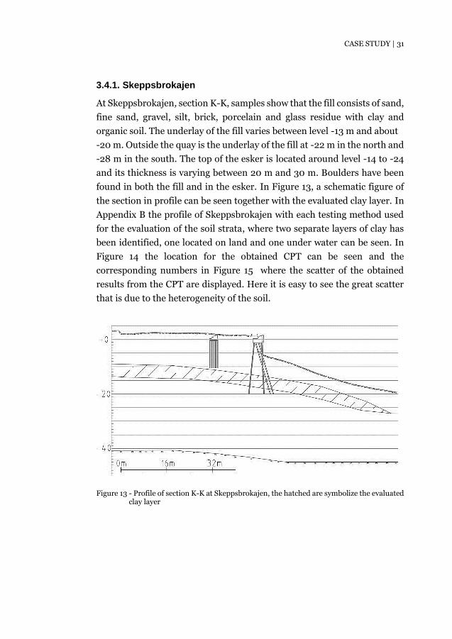
3.4.1. Skeppsbrokajen
At Skeppsbrokajen, section K-K, samples show that the fill consists of sand,
fine sand, gravel, silt, brick, porcelain and glass residue with clay and
organic soil. The underlay of the fill varies between level -13 m and about -
-20 m. Outside the quay is the underlay of the fill at -22 m in the north and
-28 m in the south. The top of the esker is located around level -14 to -24
and its thickness is varying between 20 m and 30 m. Boulders have been
found in both the fill and in the esker. In Figure 13, a schematic figure of
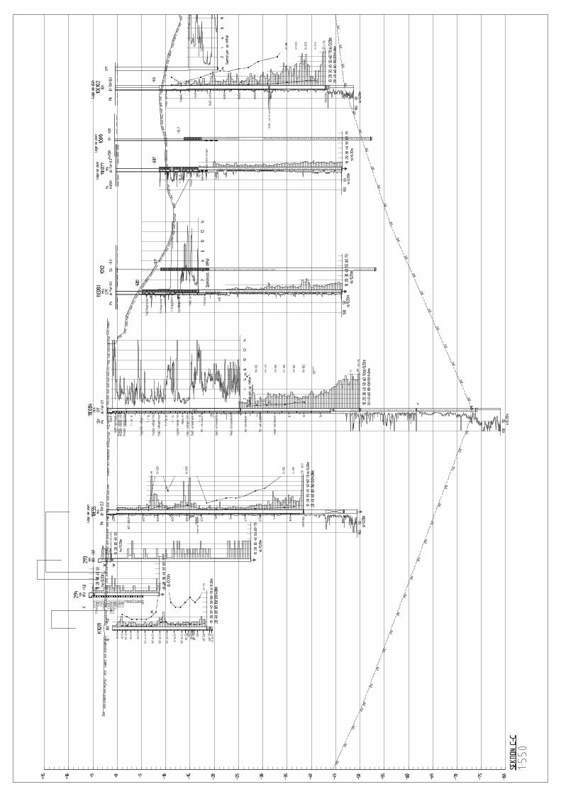
the section in profile can be seen together with the evaluated clay layer. In
Appendix B the profile of Skeppsbrokajen with each testing method used
for the evaluation of the soil strata, where two separate layers of clay has
been identified, one located on land and one under water can be seen. In
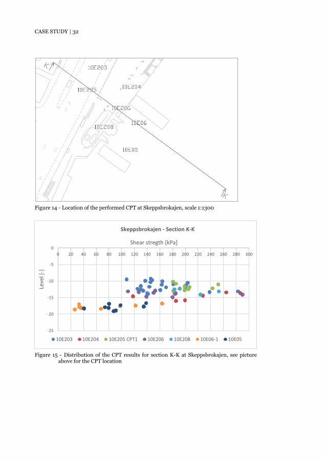
Figure 14 the location for the obtained CPT can be seen and the
corresponding numbers in Figure 15 where the scatter of the obtained
results from the CPT are displayed. Here it is easy to see the great scatter
that is due to the heterogeneity of the soil.
Figure 13 - Profile of section K-K at Skeppsbrokajen, the hatched are symbolize the evaluated clay layer
CASE STUDY | 32
Figure 14 - Location of the performed CPT at Skeppsbrokajen, scale 1:1300
Figure 15 - Distribution of the CPT results for section K-K at Skeppsbrokajen, see picture
above for the CPT location
-25
-20
-15
-10
-5
0
0 20 40 60 80 100 120 140 160 180 200 220 240 260 280 300
Leve
l [-]
Shear stregth [kPa]
Skeppsbrokajen - Section K-K
10E203 10E204 10E205 CPT1 10E206 10E208 10E06-1 10E05

CASE STUDY | 33
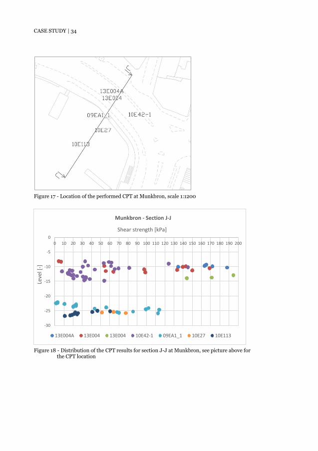
3.4.2. Munkbron
At Munkbron, section J-J, the area consists of old seabed which has
become a land area due to the isostasy and fill. The thick fill is mixed with
organic soil and clay has also been found. The fill consists of sand, gravel,
silt, glass, brick, metal, ceramic, bone, mortar, porcelain, wood etc. mixed
with clay, gyttja and mud. Underneath the filling a more cohesive layer of
soil that is undrained has been found with CPT. The main part of the esker
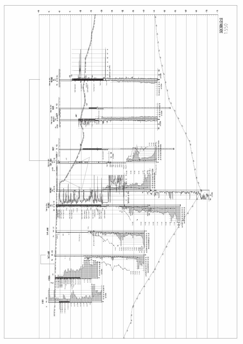
is sand and gravel upon the bedrock. In Figure 16, a schematic figure of the
section in profile can be seen together with the evaluated clay layer. See
Appendix B for the profile of Munkbron with each testing method used for
the evaluation of the soil strata. In Figure 17 the location for the obtained
CPT can be seen and the corresponding numbers in Figure 18 where the
scatter of the obtained results from the CPT are displayed.
Figure 16 - Section J-J at Munkbron, the hatched are symbolize the evaluated clay layer
CASE STUDY | 34
Figure 17 - Location of the performed CPT at Munkbron, scale 1:1200
Figure 18 - Distribution of the CPT results for section J-J at Munkbron, see picture above for
the CPT location
-30
-25
-20
-15
-10
-5
0
0 10 20 30 40 50 60 70 80 90 100 110 120 130 140 150 160 170 180 190 200
Leve
l [-]
Shear strength [kPa]
Munkbron - Section J-J
13E004A 13E004 13E004 10E42-1 09EA1_1 10E27 10E113
CASE STUDY | 35
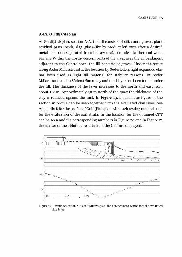
3.4.3. Guldfjärdsplan
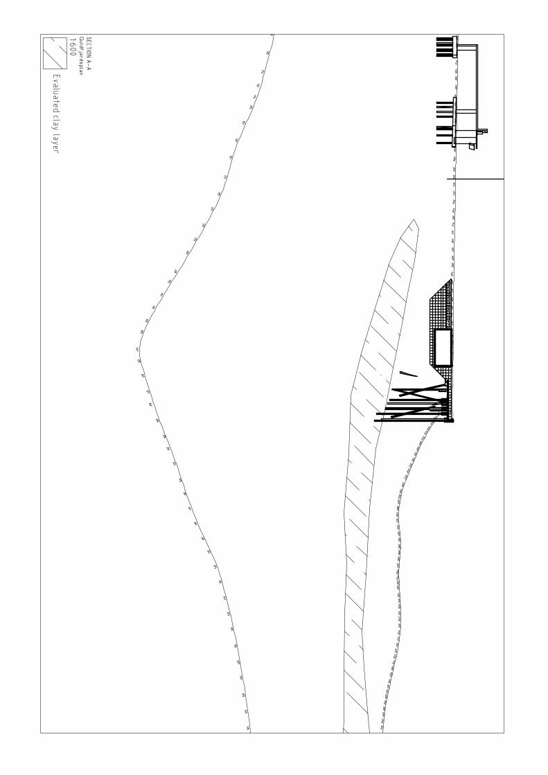
At Guldfjärdsplan, section A-A, the fill consists of silt, sand, gravel, plant
residual parts, brick, slag (glass-like by product left over after a desired
metal has been separated from its raw ore), ceramics, leather and wood
remain. Within the north-western parts of the area, near the embankment
adjacent to the Centralbron, the fill consists of gravel. Under the street
along Söder Mälarstrand at the location by Söderleden, light expanded clay
has been used as light fill material for stability reasons. In Söder
Mälarstrand and in Söderström a clay and mud layer has been found under
the fill. The thickness of the layer increases to the north and east from
about 1-2 m. Approximately 30 m north of the quay the thickness of the
clay is reduced against the east. In Figure 19, a schematic figure of the
section in profile can be seen together with the evaluated clay layer. See
Appendix B for the profile of Guldfjärdsplan with each testing method used
for the evaluation of the soil strata. In the location for the obtained CPT
can be seen and the corresponding numbers in Figure 20 and in Figure 21
the scatter of the obtained results from the CPT are displayed.
Figure 19 - Profile of section A-A at Guldfjärdsplan, the hatched area symbolizes the evaluated
clay layer
CASE STUDY | 36
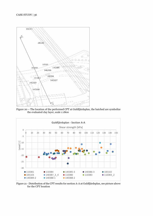
Figure 20 – The location of the performed CPT at Guldfjärdsplan, the hatched are symbolize
the evaluated clay layer, scale 1:1800
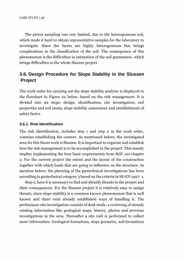
Figure 21 - Distribution of the CPT results for section A-A at Guldfjärdsplan, see picture above
for the CPT location
-30
-25
-20
-15
-10
-5
0
0 10 20 30 40 50 60 70 80 90 100 110 120 130 140 150
Leve
l [-]
Shear strength [kPa]
Guldfjärdsplan - Section A-A
11E081 11E084 14E085-3 14E086-3 10E10210E103 14E087_3_4 11E080 11E083 11E083_214E089-2 14E088-1 14E088-2

CASE STUDY | 37
3.5. Uncertainties in the Field Results from Slussen
In the surveying report (Exploateringskontoret, 2011) the possible
uncertainties are addressed which are related to the test results. The
evaluation of the soil parameters has been executed with the software
CONRAD version 3.0 together with “SGI Information 3” (Larsson, et al.,
2007) and the results can be found in “CONRAD utvärderingar”
(Exploateringskontoret, 2016). Sampling was in most cases not possible to
perform and in-situ method CPT was applied for interpretation.
Regarding the classification of the soil, the results evaluated with CPT
together with CONRAD differ from the sampling results from the same
area. In most cases it means that CONRAD evaluates part of the soil as clay
and the samples as friction soil. The sampling is rough, and the CPT may
have picked up layers that the sampling has missed. The CONRAD
evaluation is however based on empiric model for natural layered clay, silt
and sand, not for the mixed fill and esker material which are the dominant
soil within the area of Slussen. Regarding this the results from CONRAD
needs to be evaluated with caution. With low measured tip resistance,
which CONRAD normally evaluates as clay, it might be in the esker an
indicator that the material consists of highly loosely stocked boulders
which is likely to consist of single-grade and rounded grains.
In the fill this may be due to heterogeneity and the presence of parts
with, for example, silt/clay/mud or such fine ground soils are mixed
between more coarse grain fill, which reduces friction between the grains.
In natural friction soil and esker material, the low density in certain areas
may also be depending on this phenomenon.
In evaluation of the undrained shear strength with CONRAD, the
measured tip resistance and friction ratio are crucial for the soil
classification, as mentioned above, and thus also for the evaluation of
strength parameters. In derived values, only evaluated undrained shear
strength is presented where this coincides with a clearly generated pore
pressure. Strength values from CONRAD should be critically reviewed, and
the CONRAD evaluations should be considered before these values are
used as the basis for calculations.
CASE STUDY | 38
The piston sampling was very limited, due to the heterogeneous soil,
which made it hard to obtain representative samples for the laboratory to
investigate. Since the layers are highly heterogeneous this brings
complications in the classification of the soil. The consequence of this
phenomenon is the difficulties in estimation of the soil parameters, which
brings difficulties to the whole Slussen project.
3.6. Design Procedure for Slope Stability in the Slussen
Project
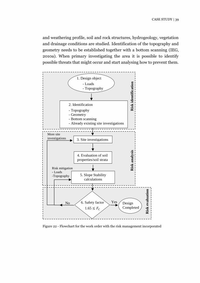
The work order for carrying out the slope stability analysis is displayed in
the flowchart in Figure 22 below, based on the risk management. It is
divided into six steps: design, identification, site investigation, soil
properties and soil strata, slope stability assessment and establishment of
safety factor.
3.6.1. Risk Identification
The risk identification, includes step 1 and step 2 in the work order,
contains establishing the context. As mentioned before, the investigated
area for this thesis work is Slussen. It is important to organise and establish
how the risk management is to be accomplished in the project. This mainly
implies implementing the four basic requirements from SGF, see chapter
2. For the current project the extent and the layout of the construction
together with which loads that are going to influence on the structure. As
mention before, the planning of the geotechnical investigations has been
according to geotechnical category 3 based on the criteria in SS-EN 1997- 1.
Step 2, here it is necessary to find and identify threats to the project and
their consequences. For the Slussen project it is relatively easy to assign
threats, since slope stability is a common known phenomenon that is well
known and there exist already established ways of handling it. The
preliminary site investigation consists of desk study, a reviewing of already
existing information like geological maps, history, photos and previous
investigations in the area. Thereafter a site visit is performed to collect
more information. Geological formations, slope geometry, soil formations
CASE STUDY | 39
and weathering profile, soil and rock structures, hydrogeology, vegetation
and drainage conditions are studied. Identification of the topography and
geometry needs to be established together with a bottom scanning (IEG,
2010a). When primary investigating the area it is possible to identify
possible threats that might occur and start analysing how to prevent them.
Figure 22 - Flowchart for the work order with the risk management incorporated
6. Safety factor
1.65 ≤ 𝐹𝐶
1. Design object
- Loads
- Topography
2. Identification
- Topography
- Geometry
- Bottom scanning
- Already existing site investigations
3. Site investigations
4. Evaluation of soil
properties/soil strata
5. Slope Stability
calculations
Design
Completed
Yes
More site
investigations
Risk mitigation
- Loads
-Topography
No
Ris
k i
den
tifi
cati
on
R
isk
an
aly
sis
Ris
k e
valu
ati
on
CASE STUDY | 40
3.6.2. Risk Analysis
The risk analysis is the complicated part of the risk management and
includes step 3, 4 and 5. The risk needs to be described with uncertainties
and severity of the consequences. The risk analyse is to provide
descriptions of the risk that can occur, in terms of probability and severity
of the consequences.
Step 3 – detailed site needs to be made, with in situ testing, boring,
sampling and later laboratory test to learn more about the soil properties
and soil profile (Ortigao & Sayao, 2004). The on-site boring and sounding
to collect information can be performed with total soil and rock drilling,
static and dynamic penetration test and cone penetration test, see Figure
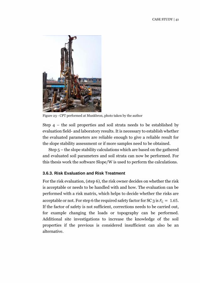
23 for performed CPT (SGF, 2013).
In the surveying report (Exploateringskontoret, 2011), field tests and
evaluated soil strata can be found for the different areas at Slussen. The
purpose of sampling soil is to obtain samples that have the least amount of
disturbance. This disturbance can come from change in stress condition,
mechanical disturbance of the soil structure, changes in water content and
porosity, chemical changes or mixing and segregation of soil constituents.
The ambition is to eliminate the changes in stress condition, mechanical
disturbance and changes in water content and porosity and to eliminate
chemical changes and mixing and segregation (Briaud, 2013).
Due to the heterogeneity in the Slussen area, sampling was limited,
since piston sampler could not be applied in most cases the in-situ method
CPT was used instead. For pictures on obtained samples, see Appendix B.
CASE STUDY | 41
Figure 23 - CPT performed at Munkbron, photo taken by the author
Step 4 – the soil properties and soil strata needs to be established by
evaluation field- and laboratory results. It is necessary to establish whether
the evaluated parameters are reliable enough to give a reliable result for
the slope stability assessment or if more samples need to be obtained.
Step 5 – the slope stability calculations which are based on the gathered
and evaluated soil parameters and soil strata can now be performed. For
this thesis work the software Slope/W is used to perform the calculations.
3.6.3. Risk Evaluation and Risk Treatment
For the risk evaluation, (step 6), the risk owner decides on whether the risk
is acceptable or needs to be handled with and how. The evaluation can be
performed with a risk matrix, which helps to decide whether the risks are
acceptable or not. For step 6 the required safety factor for SC 3 is 𝐹C = 1.65.
If the factor of safety is not sufficient, corrections needs to be carried out,
for example changing the loads or topography can be performed.
Additional site investigations to increase the knowledge of the soil
properties if the previous is considered insufficient can also be an
alternative.
CASE STUDY | 42
In risk treatment, the goal is to decrease the risk if it is considered
unacceptable by executing risk, reducing measures. Different ways of
preventing a landslide are used for this investigated case at Slussen. To
reduce and prevent a slide can be achieved by reducing the load on top of
the slope or by making a support at the slope toe which will increase the
stability.
For the six steps, it is step 4 with the evaluation of soil properties and
soil strata that holds the majority of the uncertainties. The previous steps
consist of gathering information and area characterising. The slope
stability calculations for step 5 are rather straight forward, standardized
and easy to manage. The majority of the uncertainties lies in the evaluated
properties. Due to the heterogeneity in the Slussen area and fill masses
overlaying the clay, sampling was limited, since piston sampler could not
be applied so in most cases the in-situ method CPT was used instead.
Limitations with only one test method is that it is not possible to verify if
the results are reasonable, especially with the existing complexity of the
soil. The epistemic uncertainty could be lowered with more tests since
more knowledge would be gathered about the area. However, more CPT
might only increase the range of results since the soil is highly
heterogeneous, and hence the variance. Since other test was difficult to
perform the conclusion could be that the already gathered information is
sufficient enough.

METHODOLOGY | 43
Methodology: Evaluation of Shear Strength
The aim of this thesis work is to investigate how different methods
influence the determination of the characteristic value of the shear
strength in the clay. This is essential from a risk management perspective
since the parameter have great influence on the stability and hence the
safety.
Step 4 in the work order, see Figure 22, is to determine the soil
properties and soil strata. From the area at Slussen, cross-sections
(Guldfjärdsplan, Munkbron, Skeppsbrokajen) have been chosen for the
determination of 𝑐u. The evaluation has been performed with three
approaches based on the same input data:
(I) The 5 % fractile of the mean value according to Eurocode 7
(II) The Swedish method with the η-factor according to the IEG-
report 6:2008 slopes and embankments.
(III) A questionnaire where geotechnical engineers were asked to
“estimate a cautiously assumed mean value”. Also in
accordance with Eurocode 7, Clause 2.4.5.2(2).
There are two major aspects to consider when selecting the
characteristic value: (1) the amount of, and degree of confidence in,
knowledge of the parameter values and (2) the soil volume involved in the
limit state considered and the ability of the structure to transfer loads from
weak to strong zones in the ground (Frank, et al., 2005).
4.1. (I) Eurocode 7: the 5 % Fractile
4.1.1. Background
The following section is based on “Designers guide to Eurocode 7:
Geotechnical design” (Frank, et al., 2005). The statistic formulae to
determine the 5 % fractile depend on the type of statistical population, the
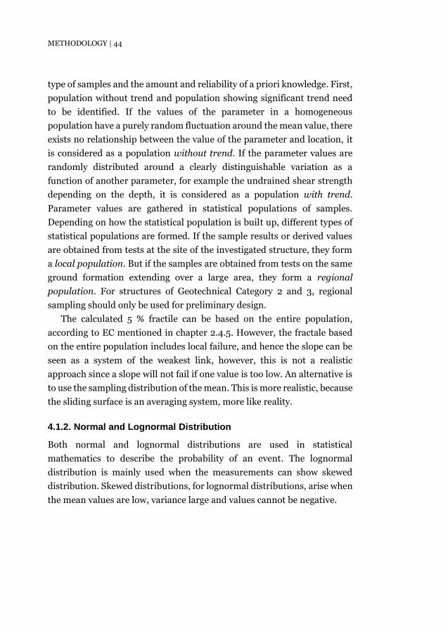
METHODOLOGY | 44
type of samples and the amount and reliability of a priori knowledge. First,
population without trend and population showing significant trend need
to be identified. If the values of the parameter in a homogeneous
population have a purely random fluctuation around the mean value, there
exists no relationship between the value of the parameter and location, it
is considered as a population without trend. If the parameter values are
randomly distributed around a clearly distinguishable variation as a
function of another parameter, for example the undrained shear strength
depending on the depth, it is considered as a population with trend.
Parameter values are gathered in statistical populations of samples.
Depending on how the statistical population is built up, different types of
statistical populations are formed. If the sample results or derived values
are obtained from tests at the site of the investigated structure, they form
a local population. But if the samples are obtained from tests on the same
ground formation extending over a large area, they form a regional
population. For structures of Geotechnical Category 2 and 3, regional
sampling should only be used for preliminary design.
The calculated 5 % fractile can be based on the entire population,
according to EC mentioned in chapter 2.4.5. However, the fractale based
on the entire population includes local failure, and hence the slope can be
seen as a system of the weakest link, however, this is not a realistic
approach since a slope will not fail if one value is too low. An alternative is
to use the sampling distribution of the mean. This is more realistic, because
the sliding surface is an averaging system, more like reality.
4.1.2. Normal and Lognormal Distribution
Both normal and lognormal distributions are used in statistical
mathematics to describe the probability of an event. The lognormal
distribution is mainly used when the measurements can show skewed
distribution. Skewed distributions, for lognormal distributions, arise when
the mean values are low, variance large and values cannot be negative.
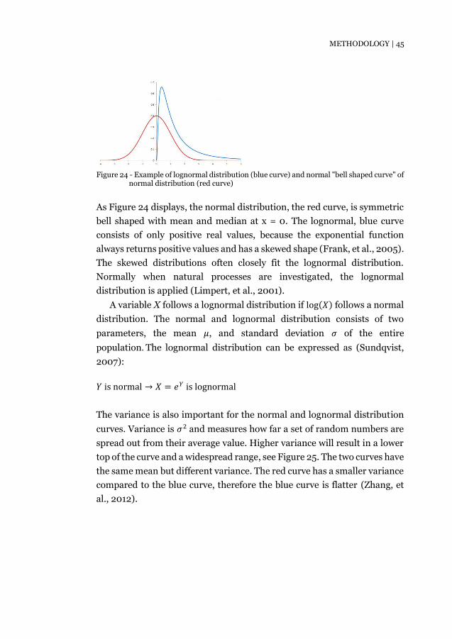
METHODOLOGY | 45
Figure 24 - Example of lognormal distribution (blue curve) and normal "bell shaped curve" of
normal distribution (red curve)
As Figure 24 displays, the normal distribution, the red curve, is symmetric
bell shaped with mean and median at x = 0. The lognormal, blue curve
consists of only positive real values, because the exponential function
always returns positive values and has a skewed shape (Frank, et al., 2005).
The skewed distributions often closely fit the lognormal distribution.
Normally when natural processes are investigated, the lognormal
distribution is applied (Limpert, et al., 2001).
A variable X follows a lognormal distribution if log(𝑋) follows a normal
distribution. The normal and lognormal distribution consists of two
parameters, the mean 𝜇, and standard deviation 𝜎 of the entire
population. The lognormal distribution can be expressed as (Sundqvist,
2007):
𝑌 is normal → 𝑋 = 𝑒𝑌 is lognormal
The variance is also important for the normal and lognormal distribution
curves. Variance is 𝜎2 and measures how far a set of random numbers are
spread out from their average value. Higher variance will result in a lower
top of the curve and a widespread range, see Figure 25. The two curves have
the same mean but different variance. The red curve has a smaller variance
compared to the blue curve, therefore the blue curve is flatter (Zhang, et
al., 2012).
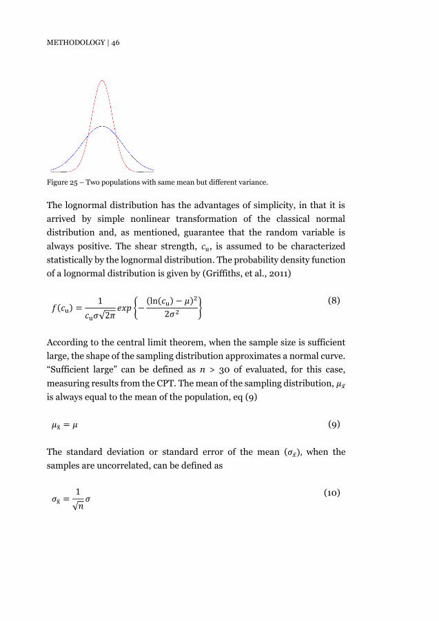
METHODOLOGY | 46
Figure 25 – Two populations with same mean but different variance.
The lognormal distribution has the advantages of simplicity, in that it is
arrived by simple nonlinear transformation of the classical normal
distribution and, as mentioned, guarantee that the random variable is
always positive. The shear strength, 𝑐u, is assumed to be characterized
statistically by the lognormal distribution. The probability density function
of a lognormal distribution is given by (Griffiths, et al., 2011)
𝑓(𝑐u) =1
𝑐u𝜎√2𝜋𝑒𝑥𝑝 {−
(ln(𝑐u) − 𝜇)2
2𝜎2}
(8)
According to the central limit theorem, when the sample size is sufficient
large, the shape of the sampling distribution approximates a normal curve.
“Sufficient large” can be defined as n > 30 of evaluated, for this case,
measuring results from the CPT. The mean of the sampling distribution, 𝜇�̅�
is always equal to the mean of the population, eq (9)
𝜇x̅ = 𝜇 (9)
The standard deviation or standard error of the mean (𝜎�̅�), when the
samples are uncorrelated, can be defined as
𝜎x̅ =1
√𝑛𝜎
(10)

METHODOLOGY | 47
were n being the sample size (number of items in the sample) (Benjamin &
Cornell, 1970).
The obtained characteristic value using 5 % fractile are then used for
calculating the design value (Frank, et al., 2005)
𝑋d = 𝑋k
1
𝛾M
(11)
4.2. (II) Swedish Method – Conversion Factor 𝜼
The “Swedish method” is based on the Swedish application document to
EC 7, “Application document – the basics of Eurocode 7” (IEG, 2010b). The
design value for geotechnical constructions, where a low value is
unfavourable, 𝑋d is calculated according to eq (12) and the characteristic
value 𝑋c with eq (13):
𝑋d =𝑋chosen∙𝜂
𝛾𝑀=
𝑋chosen
𝛾𝑀/𝜂 (12)
𝑋𝑐 = 𝜂 ∙ 𝑋chosen (13)
where 𝛾𝑀 is the constant partial factor, 𝜂 the conversion factor and 𝑋chosen
the chosen value based in derived values; in this chase it was be chosen by
me, the researcher based on the same collected data as presented in the
questionnaire and also presented in chapter 3.4.1 to 3.4.3 for each section.
The 𝜂-factor is determined based on the type of geotechnical structure.
For slopes and embankments, it is regulated according to “Application
documents – EN 1997 – 1: chapter 11 and 12, slopes and embankments”
(IEG, 2008a). The η-factor is calculated as the product of several sub-
factors:
𝜂 = 𝜂1𝜂2𝜂3𝜂4𝜂5𝜂6𝜂7𝜂8 (14)
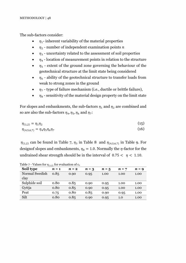
METHODOLOGY | 48
The sub-factors consider:
𝜂1- inherent variability of the material properties
𝜂2 - number of independent examination points n
𝜂3 - uncertainty related to the assessment of soil properties
𝜂4 - location of measurement points in relation to the structure
𝜂5 - extent of the ground zone governing the behaviour of the
geotechnical structure at the limit state being considered
𝜂6 - ability of the geotechnical structure to transfer loads from
weak to strong zones in the ground
𝜂7 - type of failure mechanism (i.e., ductile or brittle failure),
𝜂8 - sensitivity of the material design property on the limit state
For slopes and embankments, the sub-factors 𝜂1 and 𝜂2 are combined and
so are also the sub-factors 𝜂4, 𝜂5, 𝜂6 and 𝜂7:
𝜂(1,2) = 𝜂1𝜂2 (15)
𝜂(4,5,6,7) = 𝜂4𝜂5𝜂6𝜂7 (16)
𝜂(1,2) can be found in Table 7, 𝜂3 in Table 8 and 𝜂(4,5,6,7) in Table 9. For
designof slopes and embankments, 𝜂8 = 1.0. Normally the 𝜂-factor for the
undrained shear strength should be in the interval of 0.75 < 𝜂 < 1.10.
Table 7 - Values for 𝜂(1,2) for evaluation of cu
Soil type n = 1 n = 2 n = 3 n = 5 n = 7 n = 9
Normal Swedish
clay
0.85 0.90 0.95 1.00 1.00 1.00
Sulphide soil 0.80 0.85 0.90 0.95 1.00 1.00
Gyttja 0.80 0.85 0.90 0.95 1.00 1.00
Peat 0.75 0.80 0.85 0.90 0.95 1.00
Silt 0.80 0.85 0.90 0.95 1.0 1.00

METHODOLOGY | 49
Table 8 - Values for 𝜂3 for evaluation of cu
Influencing factors 𝜼𝟑 [-]
One method of CPT/field vane/fall cone test has been used
0.90
Two to three methods have been used, large variability in the results1
0.95
Two to three methods have been used, small variability in the results
1.0
Two to three methods have been used, large variability in the results and empirical relations2 confirm the results
1.05
Direct simple shear test or triaxial test confirm the results from other investigations and empirical relations
1.1
1 Obviously incorrect results shall be rejected. 2 Refers to empirical relations between the undrained shear strength and the preconsolidation stress evaluated from constant-rate-of-strain oedometer tests.
Table 9 - Values for 𝜂(4,5,6,7)
Extent of failure zone/ consequence of failure
Mean value/ weak zone
Distance to investigated points
𝜼(𝟒,𝟓,𝟔,𝟕)
Large failure zone Mean - 1.00 Weak zone - 0.95
Small failure zone, small consequence of failure
- - 1.00
Small failure zone, great consequence of failure
Mean Short 1.00 Long 0.95
Weak zone Short 0.95 Long 0.90
The application and possible adjustment when using the 𝜂-factor are
further discussed in Prästings, et al, article (2017), as mentioned earlier.

METHODOLOGY | 50
4.3. (III) Questionnaire Evaluation
The questionnaire was mainly distributed during “Foundation day”, the
15th mars 2018, arranged by The Swedish Geotechnical Society. It is a
conference. Also, some answers were obtained from colleague at ELU
consultant AB, where this master thesis was written.
From the three areas that were chosen, the results from CPT at or near
the chosen section was collected from the “Ground investigation report”
(Exploateringskontoret, 2011) and assembled in diagrams. From the
diagrams, geotechnical engineers were asked to evaluate a cautiously
assumed mean value of the undrained shear strength. The questionnaire
consisted of five questions; some basic data regarding the person
answering and then the main question regarding the evaluation of the
shear strength. The questionnaire can be seen in Appendix A.
The correlations that have been investigated is regarding the
“cautiously estimated mean value” and age, years of experience and
willingness to take risks. The correlation (𝑅2) describes the statistical
relationship between two variables. A 𝑅2 value close to 1 would imply
correlation between the mentioned situations and a 𝑅2 value close to zero
implies no correlation (Rodgers & Nicewander, 1988).
4.4. Safety Factors with Slope/W
For the calculations regarding slope stability the software program
Slope/W was used. The three different obtained characteristic values for
the shear strength were changed for each section in order to investigate
how they influenced the safety factor for slope stability. The assumed
values for the other soil layers was kept constant and was gained from
“Total stability research – Guldfjärdsplan, section E-E”
(Exploateringskontoret , 2017), see Table 10. The groundwater levels used
for the calculations with Slope/W for each section can be found in Table 11.
Only characteristic values have been used and the required safety factor is
𝐹𝑐 = 1.65
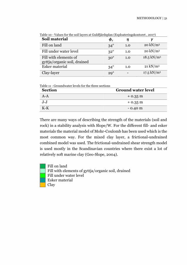
METHODOLOGY | 51
Table 10 - Values for the soil layers at Guldfjärdsplan (Exploateringskontoret , 2017)
Soil material 𝝓𝒄 𝜼 𝜸
Fill on land 34° 1.0 20 kN/m3
Fill under water level 32° 1.0 20 kN/m3
Fill with elements of gyttja/organic soil, drained
30° 1.0 18.5 kN/m3
Esker material 34° 1.0 21 kN/m3
Clay-layer 29° - 17.5 kN/m3
Table 11 - Groundwater levels for the three sections
Section Ground water level
A-A + 0.35 m
J-J + 0.35 m
K-K - 0.40 m
There are many ways of describing the strength of the materials (soil and
rock) in a stability analysis with Slope/W. For the different fill- and esker
materials the material model of Mohr-Coulomb has been used which is the
most common way. For the mixed clay layer, a frictional-undrained
combined model was used. The frictional-undrained shear strength model
is used mostly in the Scandinavian countries where there exist a lot of
relatively soft marine clay (Geo-Slope, 2004).
Fill on land Fill with elements of gyttja/organic soil, drained Fill under water level Esker material Clay

METHODOLOGY | 52
Figure 26 - Section K-K with the most critical slip surface displayed, the shear strength of 56
kPa according to the 5 % fractile.
In Figure 26 an example of how Slope/W looks when calculating the most
critical sliding surface for section K-K and a shear strength obtained from
the 5 % fractile. In the earliest limit equilibrium formulations, the
technique of circular trial slip surfaces, which is an arc (the portion of a
circle that cuts through the slope) of circle, were essential for specifying
circular slip surfaces. The method used for finding the most critical slip
surface is called Grid and Radius method. The grid above the slope is the
grid of rotation centres. By using a grid, a wide variation of different trial
slip surfaces can be specified. The red area of the grid is where the centre
of themost critical slip surfaces with different radius will be found (Geo-
Slope, 2004). A load of 30 kPa/m is applied as an extreme case (a fully
loaded concrete truck) in order to obtain a good comparison to the
unloaded situation.

RESULTS | 53
Results
Below are the results presented, first the outcome from each applied
method, secondly, a summary of the obtained characteristic shear strength
values and lastly, the calculated safety factors.
5.1. Results from the Three Methods
5.1.1. (I) Eurocodede 7: the 5 % Fractile
The red curves are for the normal distribution based on the sampling
distribution of the mean values, the purple curve is the lognormal
distribution based on the entire population. The sample size n and mean
value for the normal distribution are presented in Table 12. A summary of
the obtained values for the characteristic shear strength, which are based
on the two distributions are shown in Table 13. The graphs are then
presented in Figure 27 - Figure 30.
Table 12 – Number of samples and mean values for each section
Section Number of results, n Mean value [kPa]
A-A 72 97
J-J overlay 54 83
J-J underlay 33 58
K-K 71 163
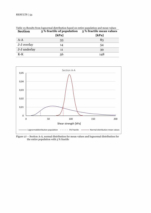
RESULTS | 54
Table 13-Results from lognormal distribution based on entire population and mean values
Section 5 % fractile of population
[kPa]
5 % fractile mean values
[kPa]
A-A 33 83
J-J overlay 14 54
J-J underlay 11 39
K-K 56 148
Figure 27 – Section A-A, normal distribution for mean values and lognormal distribution for
the entire population with 5 % fractile
0
0,01
0,02
0,03
0,04
0,05
0 50 100 150 200
Shear strength [kPa]
Section A-A
Lognormaldistribution population 5% fractile Normal distribution mean values

RESULTS | 55
Figure 28 - Section J-J overlay, normal distribution for mean values and lognormal
distribution for the entire population with 5 % fractile
Figure 29 - Section J-J underlay, normal distribution for mean values and lognormal
distribution for the entire population with 5 % fractile
0
0,005
0,01
0,015
0,02
0,025
0,03
0,035
0,04
0 50 100 150 200
Shear strength [kPa]
Section J-J overlay
Lognormaldistribution population 5 % fractile Normal distribution of the mean
0
0,005
0,01
0,015
0,02
0,025
0,03
0,035
0,04
0 50 100 150 200
Shear strength [kPa]
Section J-J underlay
Lognormaldistribution population Normal distribution of the mean
5 % fractile

RESULTS | 56
Figure 30 - Section K-K, normal distribution for mean values and lognormal distribution for
the entire population with 5 % fractile
5.1.2. (II) Swedish Method – Conversion Factor 𝜼
The calculated 𝜂-subfactors for each section and the final 𝜂-factor, Table
14 and the results of the characteristic values with the 𝜂 factor in Table 15.
𝑋chosen was subjectively determined by me, the researcher, based on the
CPT results.
Table 14 -𝜂-factor for each section, selected from Table 7 -Table 9
Section n 𝜼(𝟏,𝟐) 𝜼𝟑 𝜼(𝟒,𝟓,𝟔,𝟕) 𝜼𝟖 𝜼
A-A 13 1.0 0.9 0.95 1.0 0.86
J-J overlay 4 0.975 0.9 0.95 1.0 0.83
J-J underlay 3 0.950 0.9 0.95 1.0 0.81
K-K 7 1.0 0.9 0.95 1.0 0.86
0
0,005
0,01
0,015
0,02
0,025
0,03
0,035
0,04
0,045
0,05
0 50 100 150 200 250 300
Shear strength [kPa]
Section K-K
Lognormaldistribution population 5 % fractile
Normal distribution of the mean

RESULTS | 57
Table 15 - Results of calculated undrained shear strength
Section 𝜼 𝑿𝐜𝐡𝐨𝐬𝐞𝐧 [kPa] 𝑿𝐜 [kPa]
A-A 0.86 58 50
J-J overlay 0.83 35 29
J-J underlay 0.81 25 20
K-K 0.86 110 94
5.1.3. (III) Questionnaire
The results from the questionnaire is displayed in Figure 31. The
correlation between the safety factor and age, years of experience and
willing to take risks are displayed in Figure 32 - Figure 43 for each section
and the 𝑅2 values are presented in Table 16.
Figure 31 - Results from the questionnaire of geotechnical engineer’s estimation
50 60 7050 55
9060 45
70 55 55 72 65 60 45 4770 60 50 60 45 50
3535
50
2540
60
40
20
4035 35
30 4025
35 30
4035
20
60
25 25
3030
25
22
35
45
30
20
30
18 2028 30
3522 25
2030
20
40
2035
130140
140
145
135
180
170
140
120
120120
140150
130160135
160140
120
30
40
80
1 2 3 4 5 6 7 8 9 10 11 12 13 14 15 16 17 18 19 20 21 22
Shea
r st
ren
gth
[kP
a]
Person
People´s evaluation of shear strength
Section A-A Section J-J overlay Section J-J underlay Section K-K

RESULTS | 58
Table 16 - statistical relationship between two variables is here denoted 𝑅2
Sections 𝑹𝟐
A-A J-J overlay J-J underlay K-K
Age 0.1495 0.0035 0.0381 0.049
Experience 0.0572 0.0463 0.0067 0.29
Willingness
to risk
0.0102 0.0066 0.0001 0.0014
Figure 32 - 𝑐u correlation to age for section A-A at Guldfjärdsplan
Figure 33 - 𝑐u correlation to age for section J-J overlay at Munkbron
R² = 0,1495
0
20
40
60
80
100
22 27 32 37 42
Shea
r st
ren
gth
[kP
a]
Age
cu correlation to age - Section A-A
R² = 0,0035
0
10
20
30
40
50
60
70
22 27 32 37 42
Shea
r st
ren
gth
[kP
a]
Age
cu correlation to age - Section J-J overlay
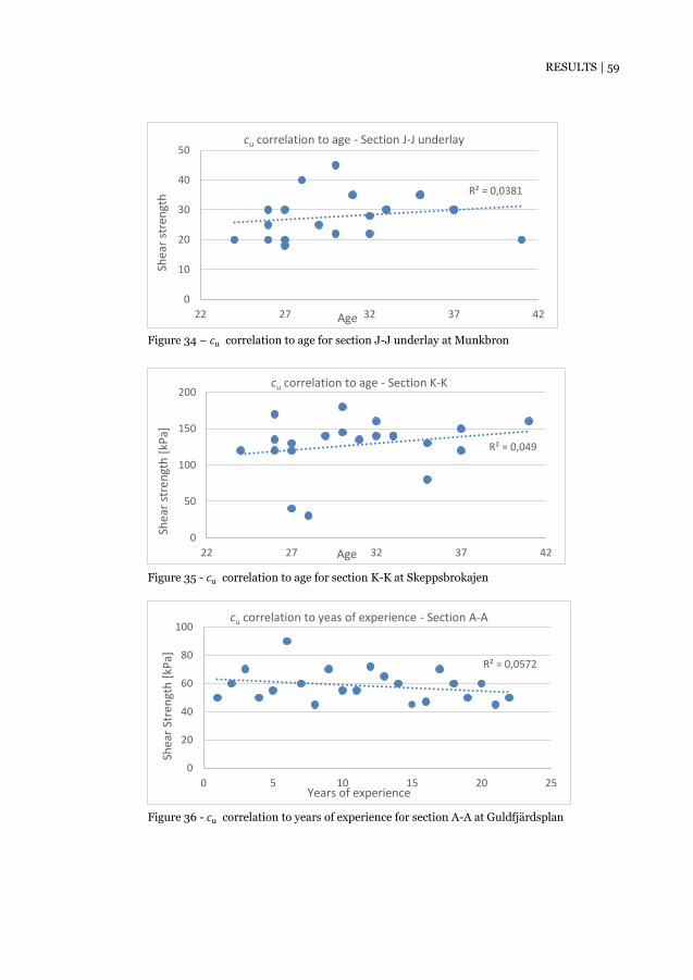
RESULTS | 59
Figure 34 – 𝑐u correlation to age for section J-J underlay at Munkbron
Figure 35 - 𝑐u correlation to age for section K-K at Skeppsbrokajen
Figure 36 - 𝑐u correlation to years of experience for section A-A at Guldfjärdsplan
R² = 0,0381
0
10
20
30
40
50
22 27 32 37 42
Shea
r st
ren
gth
Age
cu correlation to age - Section J-J underlay
R² = 0,049
0
50
100
150
200
22 27 32 37 42
Shea
r st
ren
gth
[kP
a]
Age
cu correlation to age - Section K-K
R² = 0,0572
0
20
40
60
80
100
0 5 10 15 20 25
Shea
r St
ren
gth
[kP
a]
Years of experience
cu correlation to yeas of experience - Section A-A
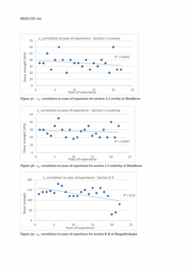
RESULTS | 60
Figure 37 – 𝑐u correlation to years of experience for section J-J overlay at Munkbron
Figure 38 - 𝑐u correlation to years of experience for section J-J underlay at Munkbron
Figure 39 - 𝑐u correlation to years of experience for section K-K at Skeppsbrokajen
R² = 0,0463
0
10
20
30
40
50
60
70
0 5 10 15 20 25
Shea
r st
ren
gth
[kP
a]
Years of experience
cu correlation to yeas of experience - Section J-J overlay
R² = 0,0067
0
10
20
30
40
50
0 5 10 15 20 25
Shea
r st
ren
gth
[kP
a]
Years of experience
cu correlation to yeas of experience - Section J-J underlay
R² = 0,29
0
50
100
150
200
0 5 10 15 20 25
Shea
r st
ren
gth
Years of experience
cu correlation to yeas of experience - Section K-K

RESULTS | 61
Figure 40 – 𝑐u correlation to willingness to take risk for section A-A
Figure 41 - 𝑐𝑢 correlation to willingness to take risk for section J-J overlay
Figure 42 - 𝑐u correlation to willingness to take risk for section J-J underlay
R² = 0,0102
0
20
40
60
80
100
1 2 3 4 5
Shea
r st
ren
gth
[kP
a]
Willingness to take risks
cu correlation to willingness to take risk - Section A-A
R² = 0,0066
0
10
20
30
40
50
60
70
1 2 3 4 5
Shea
r st
ren
gth
[kP
a]
Willingness to take risk
cu correlation to willingness to take risk - Section J-J overlay
R² = 0,0001
0
10
20
30
40
50
1 2 3 4 5
Shea
r st
ren
gth
[kP
a]
Willingness to take risk
cu correlation to willingness to take risk - Section J-J underlay

RESULTS | 62
Figure 43 - 𝑐𝑢 correlation to willingness to take risk for section K-K
5.2. Evaluated Shear Strength
The result presented in Figure 44 shows the effect of applying the three
different methods (I), (II) and (III) in the evaluation of the shear strength
in the clay layer, based on the same data obtained from CPT.
Figure 44 - Characteristic shear strength for each section with the three methods
R² = 0,0014
0
50
100
150
200
1 2 3 4 5
Shea
r st
ren
gth
[kP
a]
Willingness to take risk
cu correlation to willingness to take risk - Section K-K
50
2920
94
58
3528
128
8364
39
148
0
20
40
60
80
100
120
140
160
Section A-A Section J-J overlay Section J-Junderlay
Section K-K
Shea
r st
ren
gth
[kP
a]
Characteristic values - shear strength in clay layer
η-factor Questionnaire 5 % fractile mean values

RESULTS | 63
5.3. Calculated Safety Factors
The calculated safety factors Fc with Slope/W for characteristic values and
without applied load are displayed in Figure 45 and values are also listed
in Table 17. For the case with an applied load of 30 kPa/m see Figure 46
and Table 18. Where 𝐹c = 1.65 according to safety class 3.
Table 17 – Obtained safety factors for each method and section with no applied load
Method Section A-A Section J-J Section K-K
5% fractile mean values 2.85 1.74 1.74
η-factor 2.56 1.42 1.69
Questionnaire 2.71 1.62 1.72
Figure 45 - Safety factors for each section and method with no applied load, with required
minimum for safety class 3 of Fc = 1.65
2,56
1,421,69
2,71
1,621,72
2,85
1,741,74
0
0,5
1
1,5
2
2,5
3
Safe
ty F
acto
r
Safety Factors - Characteristic values and no applied load
Minimum Safety Factor 1.65 η-factor Questionnaire 5% fractile mean values
Section A-A Section J-J Section K-K

RESULTS | 64
Table 18 - Obtained safety factors for each method and section with an applied load Section A-A Section J-J Section K-K
5 % fractile mean values 2.35 1.55 1.57
η-factor 2.01 1.30 1.53
Questionnaire 2.18 1.36 1.56
Figure 46 - Safety factors for each section and method and with an applied load of 30 kPa/m,
with required minimum for safety class 3 of Fc = 1.65
2,01
1,30 1,53
2,18
1,36
1,56
2,35
1,55
1,57
0
0,5
1
1,5
2
2,5
Safe
ty F
acto
r
Safety Factors - Characteristic values and applied load of 30 kPa/m
Minumum safety factor 1.65 η-factor Questionnaire 5 % fractile mean values
Section A-A Section J-J Section K-K

DISCUSSION | 65
Discussion
The aims of this master thesis were to investigate and compare three
methods regarding the determination of the characteristic value of the
shear strength. The first method was based on EC 7 and the 5 % fractile,
the second on the Swedish national annex with the conversion factor 𝜂 and
the last one on geotechnical engineers’ own estimations, which were
investigated with a questionnaire.
For the case study, three sections at Slussen were investigated and the
results came from CPT performed at three locations. The soil strata in
Slussen are complicated and have heterogeneous soil layers which makes
it difficult to categorise the soil and hence evaluate the soil properties.
The method that was based on pure data and statistic, the 5 % fractile
and based on the mean values it resulted in the highest shear strength. The
questionnaire, which only depend on the engineer’s knowledge and
experience and take no further consideration to uncertainties resulted in
the second highest shear strength. For the Swedish approach, both based
on data and a methodology together with subjective judgement presented
second lowest values, see Figure 44.
In accordance with the characteristic values of the shear strength, the
safety factors are affected by the results. The highest shear strength,
obtained from the 5 % fractile based on mean values, gives the highest
safety factor, and the lowest values, from the Swedish approach with 𝜂
factor, hence results in the lowest.
6.1. Obtained Safety Factors
For the sections with no applied load, section A-A and section K-K will
obtain a sufficient safety factor (Fc > 1.65), A-A with a margin and K-K just
above the limit. Section J-J will never be considered safe (Fc < 1.65), except
for when the undrained shear strength evaluated with the 5 % fractile based
on the mean. For the sections when a load of 30 kPa/m is applied, only
section A-A for the methods with 5 % fractile based on mean, 𝜂-factor and
questionnaire will result in an adequate safety factor. The rest of the

DISCUSSION | 66
sections with the applied methods will be below the required safety factor.
This shows that the uncertainties are mainly in the estimation of the
undrained shear strength, since the slope stability calculations will not
change.
6.2. Correlations from the Questionnaire
The aim with the questionnaire was to investigate geotechnical engineers’
subjective judgement for the evaluation of the undrained shear strength.
No direct correlation regarding age of the engineer, yeas in the business or
willingness to take risks, can be seen from the results regarding the
questionnaire. 𝑅2 close to 1 would have indicated a good correlation, but
only low values were obtained for all sections and relationships to the shear
strength. For section A-A with the correlation between the shear strength
and age, the highest 𝑅2 was obtained, but since it is still low and even lower
for the other two sections no direct correlation can be drawn from age and
safety factors. The other relationships, shear strength vs years of
experience, which would seem as most likely, no correlation was notable,
and the same for shear strength vs willing to take risk.
6.3. Characteristic values
The statistical technique aims to calculate a characteristic value from the
sample parameters. The value is selected such that there is only a small
probability that the value governing the limit state in the ground will be
less favourable than the characteristic value (Frank, et al., 2005). The 5 %
fractile based on the lognormal distribution for the entire population
results in the lowest characteristic value which is to be expected because
the definition considers the probability of local failure. These values are too
low to be realistic, as the slope then is seen as a system of weakest link
unlike reality. The slope will not fail only because one value is too low, in
reality it the application of mean value are more realistic. Therefore, these
results should not be used, because they are not a realistic model of reality
and the values has not been taken into consideration for the safety

DISCUSSION | 67
assessment. According to EC 7 a more correct approach is to use the 5 %
fractile based on sampling distribution of the mean. As mentioned, this is
more like reality, because the slope failure depends on the average value of
𝑐u along the slip surface. The characteristic value estimated based on the
mean becomes closer to the sample mean as the number n of test results
increases. The A-A and K-K section have the highest n (72 and 71
respectively) and the evaluated results are also percentage closer to the
mean than section J-J (with n around 40). However, it can be discussed
weather to consider the CPT results as independently and uncorrelated
evaluated results, since some of them are from the same CPT point. If they
would be seen as correlated, the number of individual CPT tests would be
n and then it would be too low (n < 10) and the method would not be
applicable. For n < 30 the student t-distribution should be applied. The
student t-distribution is used when estimating the mean of a normally
distributed population in situations where the sample size is small
(Grigelionis, 2013). To investigate the samples correlation the spatial
variability in the soil would require further investigations. Clearly, the
larger scatter in the results obtained from heterogeneous soils, the greater
the uncertainties about the true value governing the ground. The margin
between the selected characteristic value and the mean value of the test
results will be larger if the test results shows a large scatter. Since the soil
is highly heterogeneous, uncertainties need to be incorporated more
rationally and caution to be taken when determining a value. A value so
close to the mean value would not be realistic.
A source for uncertainties and errors, is transformation uncertainties,
discussed in chapter 2.1. CPT can be badly calibrated for great shear
strength, which can induce a relative large transformation error for the
bias. Due to this, an extra margin of safety could be to prefer for the 5 %
fractile. More CPT would not decrease the transformation uncertainties. In
this thesis work, no regard to this transformation uncertainty have been
considered.
The characteristic values calculated with the conversion factor yield
values that are reduced since 𝜂 < 1 for each section. It also takes the
engineer’s risk assessment into consideration since 𝑋chosen is a subjectively

DISCUSSION | 68
estimated value, assessed based on the geotechnical engineer’s experience
and knowledge. However, the method using η-factor is not robust since it
is influenced by a large quantity of subjective judgements from the
engineer. The engineer not only needs to estimate 𝑋chosen, but also needs
to make number of selections regarding the sub-factors of 𝜂 and many of
these decisions are made without any sharp limits. More samples and in-
situ tests used to investigate the soil volume would increase the knowledge
and reliability in the obtained values, and also 𝑥chosen.
Second highest value was given by the questionnaire and a possible
reason for this is that there is no consideration taken to uncertainties
except the engineer’s knowledge and experience. Geotechnical engineers
answering the questionnaire may know too little about the area to be able
to evaluate it properly and thereby do not incorporate the right amount of
uncertainties. Since Slussen has a very complex soil profile and the soil is
highly heterogeneous, the values from the CPT have large fluctuation and
makes it more difficult for people to make a good evaluation. This method
resulted in the values with highest amount of uncertainties, since no
regards to uncertainties has been taken for example with partial
coefficients. There are only the engineers own subjective judgement and
risk assessment. Therefore, the risk will increase, which would lead to more
investigation of the soil is required and time and the cost will increase.
The method with 5 % fractile according to Eurocode is purely based on
statistics and math. No interpretation of the site and site conditions.
Depending on which distribution that is applied either unrealisticly low
values or probably too high was evaluated. The questionnaire regards the
site and the great scatter of the results, but do not incorporate uncertainties
in a rational or reliable way. They are only evaluated by the engineer
subjectively and as mentioned are not correlated to any other factor.
Therefore the Swedish approach are the more reliable, it takes the
subjective judgement into consideration, where the site and knowledge of
the location can be weighed in and the uncertainties are handled in the 𝜂-
factor.

DISCUSSION | 69
6.4. Design values
For the design values, the uncertainties included in 𝛾M are limited when
using Eurocode 7, since the factor is fixed in the equation, see eq (9).
However, the Swedish approach, where 𝜂 < 1 for all the sections, implies
an increase of the uncertainties accounted for in 𝛾M, see eq (10), since the
variable part η is included to adjust for the level of uncertainties in the
material property. The safety margin for the design values via the partial
factor 𝛾M = 1.5 for the Eurocode approach, and for the Swedish national
annex, it is for this case study increased to 𝛾M/𝜂 ≈ 1.8 due to only one type
of in-situ test (CPT), the low numbers of sample points and the large failure
zone that is considered week. Increase of the sample points together with
additional in-situ methods would lead to a lower safety margin for the
design values via the partial factor quota 𝛾M/𝜂 and leading to a higher
design value for the shear strength. Hence, the safety would increase but
that might lead to a potential financial setback for the construction if it is
oversized and for the increase of investigations regarding the soil volume.
However, it can be mentioned that in Sweden, 𝛾M = 1.5 is not officially
been determined since here 𝜂 factor is included. Therefore, it is not entirely
correct to assume 1.5 för the 5 % fractile for determining a design value
even if Sweden would choose to use this method.
However, more samples and methods used to investigate the soil
volume would increase the reliability in the obtained values, 𝑥chosen. This
could potentially be lowered with more knowledge and the design value
might not change that much, but it will come at a cost of money and time.
The reliability in the safety calculation will hence also increase with more
investigations with beneficial consequences from a risk management
perspective.
6.5. Uncertainties and Risk Management
The aleatoric uncertainties can never be reduced because they are related
to inherent spatial variability in the soil. But the epistemic uncertainties
are relating to our ability to understand, measure and describe the system

DISCUSSION | 70
under study and can be reduced with increased knowledge. To decrease the
epistemic uncertainties and increase the confidence in the slope analyse
more field and laboratory test would be to prefer to verify the CPT for the
case study. The geotechnical risk management provides a general
procedure for how to manage uncertainties that may threaten defined goals
in geotechnical engineering projects. Since the soil strata at Slussen are
complex and highly heterogeneous, this leads to greater uncertainties for
the evaluation of soil properties, which can be reduced by increasing the
knowledge of the soil. However, you might reach a point when no new
information and conclusions can be obtained, and you will not learn
anything new that will decrease the uncertainties. And we cannot obtain
any new relevant information and instead only lose money and time. To
find the balance between this is the challenge for the risk owner.
As mentioned in section 3.5 the geotechnical engineers working on
Slussen are aware of possible uncertainties related with the test results.
Regarding the classification of the soil, the results evaluated with CPT
together with CONRAD differ from the sampling results from the same
area. The evaluation of the soil properties is based on empiric model for
natural layered clay, silt and sand, not for the heterogenic filling and esker
material which are the dominant soil type within the area of Slussen. The
obtained soil properties need to be estimated with caution and awareness
about this needs to be taken in the risk management. The evaluation of
shear strength is important from a slope stability perspective since this
parameter highly affects the safety factor; if the shear strength is wrong,
then the safety factor will be affected. Increasing the number of CPTs might
not give any new information. It would probably only increase the variance
and not result in a more reliable evaluated undrained shear strength due
to the spatial variety of the heterogeneous soil.
A limitation and a weakness with his thesis work is that spatial
variability has not been taken into consideration. As mentioned above the
spatial variability influence how n is interpreted. It has also been
recognized by some researchers the importance of spatial correlation and
local averaging of statistical properties, but the phenomenon is still absent
for many probabilistic slope stability analyses. Griffiths et al discuss this in

DISCUSSION | 71
several reports (Griffiths, et al, 2009; Griffiths & Fenton, 2004; Griffiths,
et al, 2011) when spatial variability is ignored by implicitly assuming
perfect correlation can lead incorrect estimations of the probability of slope
failure. Ignoring the spatial variation will lead to conservative estimates of
the probability of slope failure. By incorporating the spatial variability, a
more reliable analyse can be performed and hence the risk analysis will be
improved.


CONCLUSION | 73
Conclusions and Suggestion for Further
Research
From the questionnaire it can be concluded that it is only a direct subjective
judgement in the evaluation of the undrained shear strength in this case
study. No other variable like years of experience and willingness to take
risk seems to influence the evaluation. This could be a topic for further
research, to investigate a larger group of selection and other possible
factors for correlation.
For heterogeneous soils a method for evaluation of soil parameters with
subjective judgement and a factor that takes uncertainties into account
would be preferable. As mentioned there exist different uncertainties that
can and will affect the results. A method that does overlook the
uncertainties, is reliable and have some degree of subjective judgement
would be desirable. Regarding Griffith’s et al discussion of spatial
variability, it seems necessary to also incorporate it in a reliability way in
order to be able to ensure good risk management and more reliable slope
stability analysis.
Based on the results in this thesis work the Swedish approach with 𝜂
factor would be to prefer. For further research, a method with a small part,
but still some influence by subjective judgement of the engineer and still
regarding uncertainties in a rational way with some factor would be
preferred. The suggestions in Prästings, et al (2017) of a more rational
procedure of managing uncertainties in design with partial factor based on
the Bayesian methodology could be one way to allow consideration of the
spatial variability. Clearly this is an area that will require more substantial
research to find the best applicable approach for estimation of soil
parameters.


REFERENCES | 75
8. References
AB Storstockholms Lokaltrafik. (2016). Fakta om SL och länet 2015.
Stockholm .
Abramson, L., Lee, T., Sharma, S., & Boyce, G. (2002). Slope stability and
stabilization methods. New York: John Wiley & Sons Inc.
Apel, H., Thieken, A. H., Merz, B., & Blöschel, G. (2004). Flood risk
assessment and associated uncertainty. Natural Hazards and
Earth System Sciences, 4(2), pp. 295-308.
Arnold, P., Fenton, G. A., Hicks, M. A., Schweckendiek, T., & Simpson, B.
(2013). Modern geotechnical design codes of practice (Vol. 1).
Amsterdam: IOS Press BV.
Benjamin, J., & Cornell, A. (1970). Probability, statistics and decision for
civil engineers . New York: Dover publications inc.
Blom, H. ( ). Slussenområdets bebyggelse i äldre tider.
Briaud, J.-L. (2013). Geotechnical engineering: Unsaturated and
saturated soils. New Jersey: John Wiley & Sons Inc.
CEN. (2002). EN 1990:2002, Eurocode - Basis of structural design.
Bryssel: CEN.
CEN. (2004). Geotechnical design. Part 1: General rules. Bryssel:
European Committee for Standardization.
EKS. (2013). Boverkets föreskrifter och allmänna råd om tillämpning av
europeiska konstruktionsstandarder (eurokoder) - BFS 2013:10 -
EKS 9. Karlskrona: Boverket.
Exploateringskontoret . (2017). Totalstabilitetsutredning -
Guldfjärdsplan, sektion E-E. Stockholm: Stockholm Stad.
Exploateringskontoret. (2011). Markteknisk undersökningsrapport,
MUR/Geoteknik och berteknik. Stockholm: Stockholms Stad.
Exploateringskontoret. (2016). CONRADutvärderingar: Bilaga 7.
Stockholm: Stockholm Stad.
REFERENCES | 76
Fenton, G., & Griffiths, D. V. (2008). Risk assessment in geotechnical
engineering. New Jersey: John Wiley & Sons, Inc.
Foster and Partners. (2018). Slussen masterplan. (Foster and Partners)
Retrieved Januari 26, 2018, from
https://www.fosterandpartners.com/projects/slussen-
masterplan/
Frank, R., Bauduin, C., Driscoll, R., Kavvadas, M., Ovesen, N. K., Orr, T., &
Schuppener, B. (2005). Designers guide to Eurocode 7:
Geotechnical design. London: ICE Publishing.
Fredlund, D. G. (1984). Analytical methods for slope stability analysis.
229-250.
Geo-Slope. (2004). Stability modeling with GeoStudio. Toronto: Geo-
Slope International.
Griffiths, D., & Fenton, G. A. (2004). Probabilistic slope stability analysis
by finite elements. Journal of Geotechnical and
Geoenvironmental Engineering, 130(5), 507-518.
Griffiths, D., Huang, J., & Fenton, G. A. (2009). Influence of spatial
variability on slopes reliability using 2-D random fields. Journal
of Geotechnical and Geoenvironmental Engineering, 135(10),
1367-1378.
Griffiths, D., Huang, J., & Fenton, G. A. (2011). Probabilistic infinite slope
analysis. Computers and Geotechnics, 38(4), 577-584.
Grigelionis, B. (2013). Student’s t-distribution and related stochastic
processes. Vilnius: Springer Berlin Heidelberg.
IEG. (2008a). EN 1997-1 Kapitel 11 och 12, slänter och banker 6:2008.
Stockholm: Implementation Commission for European Standards
in Geotechnology.
IEG. (2008b). Tillämpningsdokument - Dokumenthantering. Stockholm:
Implementation Commission for European Standards in
Geotechnology.
IEG. (2010a). Dimensionering av geokonstruktioner - Del 2:
Marktekniska undersökningar. Stockholm: Implementation
Commission for European Standards in Geotechnology.

REFERENCES | 77
IEG. (2010b). Tillämpningsdokument - Grunder i Eurokod 7 2:2008.
Stockholm: Implementation Commission for European Standards
in Geotechnology.
ISO. (2009). ISO 31000: Risk management — Principles and guidelines.
Geneva: International Organisation for Standardization .
Janbu, N. (2001). Slope stability procedures used in landslide evaluations
in practice. Journal of the Japan Landslide Society, 38(3), 161-
168.
Larsson, R. (1990). Report no 38: Behaviour of organic clay and gyttja.
Linköping: Swedish Geotechnical Institute.
Larsson, R. (2008). Information 1: Jordens egenskaper. Linköping:
Swedish Geotechnical Institute.
Larsson, R., Sällfors, G., Bengtsson, P.-E., Alen, C., Bergdahl, U., &
Eriksson, L. (2007). Information 3: Skjuvhållfasthet -
utvärdering i kohesionsjord. Linköping: Swedish Geotechnical
Institute.
Limpert, E., Stahel, W., & Abbat, M. (2001). Log-normal distributions
across the sciences: keys and clues. Oxford: BioScience.
Lorentzi, M., Olgarsson, P., & Fredriksson, G. (2005). Slussen - 1935 års
anläggning. Stockholm: Stockholms Stadsmuseum,
kulturmiljöavdelningen.
Morgenstern, N., & Price, V. (1965). The analysis of the stability of general
slip surfaces. London: The Institution of Civil Engineers.
Orr, T. L., & Day, P. (2002). Survey of geotechnical investigation methods
and determination of parameter values. Kamakura, Japan: Proc.
of Foundation Design Codes and Soil Investigation in View of
International Harmonization and Performance-Based Design.
Orr, T. L., & Farrell, E. R. (2012). Geotechnical design to Eurocode 7.
Dublin: Springer London Ltd.
Ortigao, J., & Sayao, A. S. (2004). Handbook of slope stabilisation. New
York: Springer-Verlag Berlin Heidelberg.
REFERENCES | 78
Phoon, K.-K., & Kulhaway, F. H. (1999). Evaluation of geotechnical
property variability. Canadian Geotechnical Journal, 36(4), 625-
639.
Potts, D., & Zdravovic, L. (2012). Accounting for partial material factors in
numerical analysis. Geotechnique, 62(12), 1053-1006.
Prästings, A. (2016). Aspects of probabilistic approach to desig: from
uncertainties in pre-investigation to final design. Stockholm:
KTH.
Prästings, A., Spross, J., Müller, R., Larsson, S., Bjureland, W., &
Johansson, F. (2017). Implementing the extended multivariate
approach in design with partial factors for a retaining wall in clay.
American Society of Civil Engineers, 3(4).
Rodgers, J. L., & Nicewander, A. (1988). Thirteen ways to look at the
correlation coefficient. The American Statistician, 42(1), 59-66.
Schnaid, F. (2009). In situ testing in geomechanics: the main test.
London: Taylor & Francis.
SGF. (2013). Geoteknisk fälthandbok. Göteborg: Swedish Geotechnical
Society.
SGF. (2017). Risk management in geotechnical engineering projects -
requirements: Methodology. Linköping: Swedish Geotechnical
Society.
SIS. (2010). Eurocode 7: Geotechnical design – Part 1: General rules.
Stockholm: Swedish Standards Instirute .
Spross, J., Olsson, L., & Stille, H. (2018). The Swedish Geotechnical
Society’s methodology for risk management: a tool for engineers
in their everyday work. Georisk: Assessment and Management of
Risk for Engineered Systems and Geohazards, 12(3), 183-189.
SSSC. (1995). Anvisningar för slätstabilitetsutredningar. Linköping:
Swedish Slope Stability Commission.
Stockholms Stad. ( ). Slussområdets topografi och geotekniska struktur
samt därav betingade åtgärder för viadukternas grundläggning.
Stockholm : Stockholms Stad.

REFERENCES | 79
Stockholms Stad. (2014). Lägesredovisning för Slussen. Retrieved Mars
23, 2018, from http://bygg.stockholm.se/-/Nyheter/Slussen-
/Lagesredovisning-for-Slussen/
Stockholms Stad. (2017). Slussen anpassas till dagens behov. Retrieved
November 29, 2017, from
http://vaxer.stockholm.se/projekt/slussen/slussen-
klimatanpassas2/
Sun, S., Fu, G., Djordjevic, S., & Khu, S.-T. (2012). Separating aleatory and
epistemic uncertainties: Probabilistic sewer flooding evaluation
using probability box. Jurnal of Hydrology, 420-421, pp. 360-372.
Sundqvist, H. (2007). Safety, loads and distribution on structures (Vol. 4).
Stockholm: KTH Royal Institute of Technology.
Swedish Transport Administration. (2011). TK Geo 11: Trafikverkets
tekniska krav för geokonstruktioner. Stockholm: Swedish Road
Administration.
Terzaghi, K. (1944). Theoretical soil mechanics (Vol. Second). New York:
Wiley.
Terzaghi, K., & Peck, R. B. (1948). Soil mechanics in engineering practice
. New York: John Wiley & Sons Inc.
Zhang, Y., Wu, H., & Cheng, L. (2012). Some New Deformation Formulas
about Variance and Covariance. (pp. 987-992). Wuhan:
Proceedings of 4th International Conference on Modelling,
Identification and Contro.


APPENDIX
Appendix A
Questionnaire Evaluation
The investigated area is Slussen, where three different sections have been
removed, A-A, J-J and K-K. The examined layer in each section is the clay,
where results from CPT are compiled in graphs. The task is to assume a
cautious mean of the shear strength for each section, so the results then
can be analyzed depending on the distribution of people’s assessment.
Questions
Female
Male
Age: __________
Years of experience in the construction industry: ______________
What is your role in the geotechnical industry?
Contractor
Client
Consultant
Other

APPENDIX
Make a cautiously estimation of the mean value for the undrained shear
strength based on the information for each section.
Section Cautious estimation of mean value of
the undrained shear strength
A-A
J-J Overlay clay Underlay clay
K-K
How willing are you to take risks (1 is little and 5 is a lot)?
1 2 3 4 5
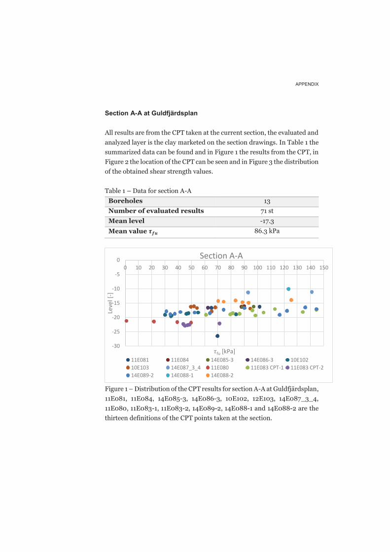
APPENDIX
Section A-A at Guldfjärdsplan
All results are from the CPT taken at the current section, the evaluated and
analyzed layer is the clay marketed on the section drawings. In Table 1 the
summarized data can be found and in Figure 1 the results from the CPT, in
Figure 2 the location of the CPT can be seen and in Figure 3 the distribution
of the obtained shear strength values.
Table 1 – Data for section A-A
Boreholes 13
Number of evaluated results 71 st
Mean level -17.3
Mean value !"# 86.3 kPa
Figure 1 – Distribution of the CPT results for section A-A at Guldfjärdsplan,
11E081, 11E084, 14E085-3, 14E086-3, 10E102, 12E103, 14E087_3_4,
11E080, 11E083-1, 11E083-2, 14E089-2, 14E088-1 and 14E088-2 are the
thirteen definitions of the CPT points taken at the section.
-30
-25
-20
-15
-10
-5
0
0 10 20 30 40 50 60 70 80 90 100 110 120 130 140 150
Leve
l [-
]
!fu [kPa]
Section A-A
11E081 11E084 14E085-3 14E086-3 10E102
10E103 14E087_3_4 11E080 11E083 CPT-1 11E083 CPT-2
14E089-2 14E088-1 14E088-2
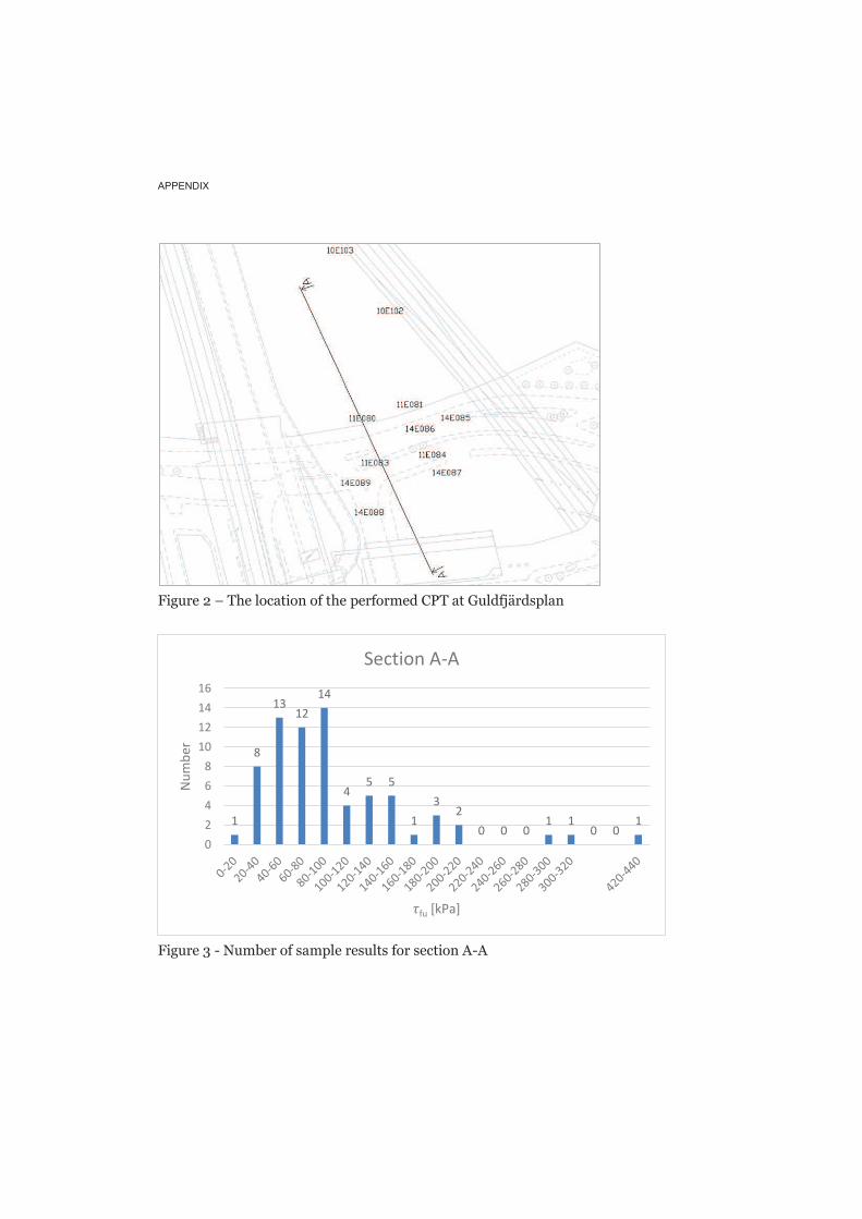
APPENDIX
Figure 2 – The location of the performed CPT at Guldfjärdsplan
Figure 3 - Number of sample results for section A-A
1
8
1312
14
45 5
1
32
0 0 01 1
0 01
0
2
4
6
8
10
12
14
16
Nu
mb
er
!fu [kPa]
Section A-A

APPENDIX
Section J-J at Munkbron
All results are from the CPT taken at the current section, the evaluated and
analyzed layer is the clay marketed on the section drawings. In Table 2the
summarized data can be found and in Figure 4 the results from the CPT, in
Figure 5 the location of the CPT can be seen and in Figure 3 the distribution
of the obtained shear strength values.
Table 2 - Data for section J-J
Boreholes 7
Number of evaluated results 87
Mean level -16.4
Mean value !"# 73.6 kPa
Figure 4 - Distribution of the CPT results for section J-J at Munkbron,
13E004A-2, 13E004-2, 13E004, 10E42-1, 09EA1_1, 10E27-2, 10E113-2 are
the seven definitions of the CPT points taken at the section.
-30
-25
-20
-15
-10
-5
0
0 10 20 30 40 50 60 70 80 90 100110120130140150160170180190200
Leve
l [-
]
!fu [kPa]
Section J-J
13E004A CPT2 13E004 CPT2 13E004 10E42-1
09EA1_1 10E27 CPT2 10E113 CPT2

APPENDIX
Figure 5 - Location of the performed CPT at Skeppsbrokajen
Figure 6 - Number of sample results for section J-J
7
9
5 5
23
2
10
13
65
34 4
5
21 1
0
2
4
6
8
10
12
14
Nu
mb
er
!fu [kPa]
Section J-J
Undre lerlager övre lerlager

APPENDIX
Section K-K at Skeppsbrokajen
All results are from the CPT taken at the current section, the evaluated and
analyzed layer is the clay marketed on the section drawings. In Table 3 the
summarized data can be found and in Figure 7 the results from the CPT, in
Figure 8 the location of the CPT can be seen and in Figure 3 the distribution
of the obtained shear strength values.
Table 3 - Data for section K-K
Boreholes 7
Number of evaluated results 72
Mean level -13.9
Mean value !"# 170.9 kPa
Figure 7 - Distribution of the CPT results for section K-K at
Skeppsbrokajen, 10E203, 12E204, 10E205-1, 10E206, 10E208, 10E06-1,
10E05 are the seven definitions of the CPT points taken at the section.
-25
-20
-15
-10
-5
0
0 20 40 60 80 100 120 140 160 180 200 220 240 260 280 300
Leve
l [-
]
!fu [kPa]
Section K-K
10E203 10E204 10E205 CPT1 10E206 10E208 10E06-1 10E05
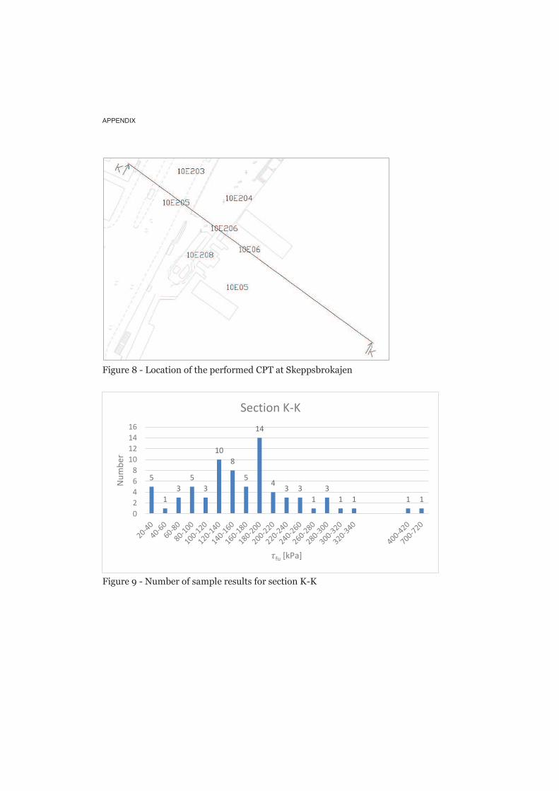
APPENDIX
Figure 8 - Location of the performed CPT at Skeppsbrokajen
Figure 9 - Number of sample results for section K-K
5
1
3
5
3
10
8
5
14
43 3
1
3
1 1 1 1
0
2
4
6
8
10
12
14
16
Nu
mb
er
!fu [kPa]
Section K-K
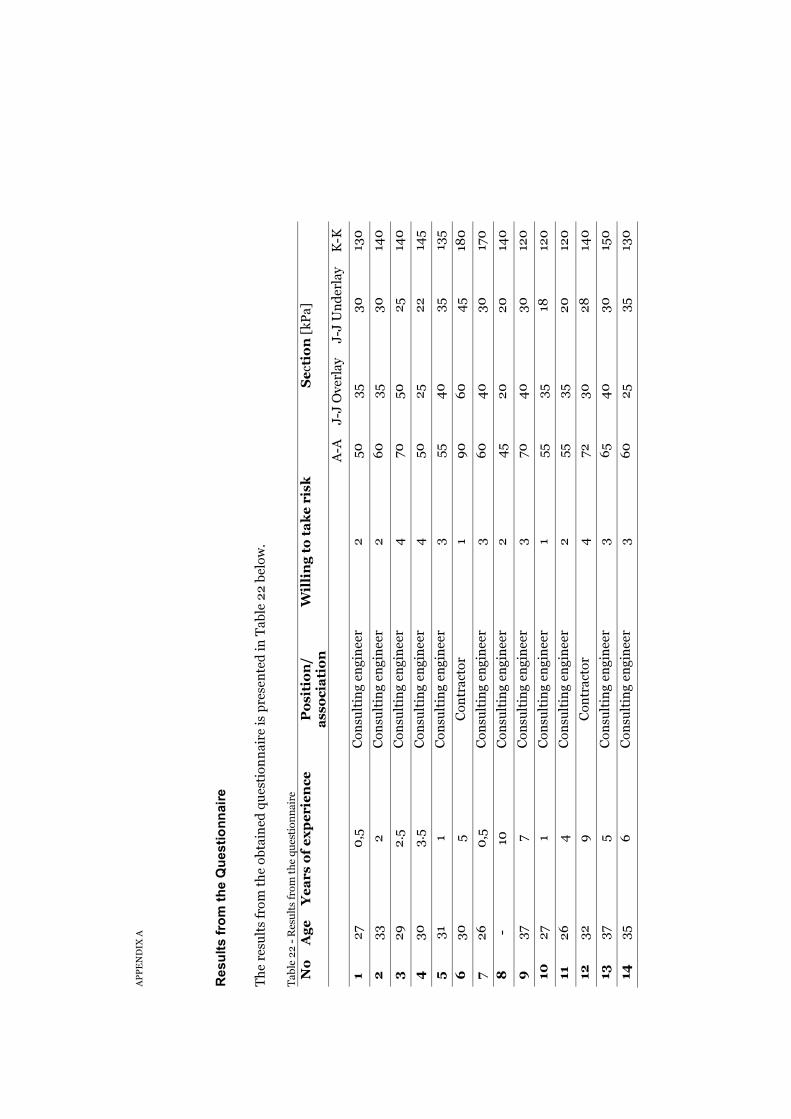
Re
su
lts f
rom
th
e Q
ues
tio
nn
air
e
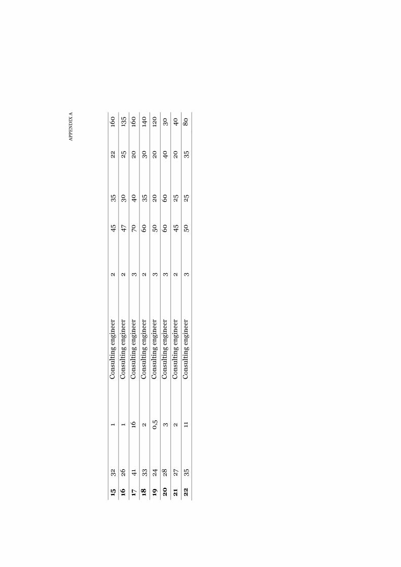

APPENDIX
Appendix B
Profiles of the Investigated Sections
Pictures showing samples taken of the soil strata at Slussen. A mix of sand,
gravel and clay/mud/gyttja with organic content, showing the complexity
and variation that exist in the soil for the area, see Figure 10 and Figure 11.
On the following pages the profiles for each section is presented. First
each section with the sampling results and after that, the evaluation of the
extent for the clay layer. The performed test definitions can be seen in
Table 4. Section A-A is evaluated from section C-C and section D-D at
Guldfjärdsplan.
Table 4 -Performed test for the sections
Hfa Standard penetration test
Jb Total soil-rock drilling
CPT Cone penetration test
Figure 10 – Samples taken at Slussen. Left: Clay/mud/gyttja with organic material with
some rocks Middle: Sand with some rocks. Right: Organic material
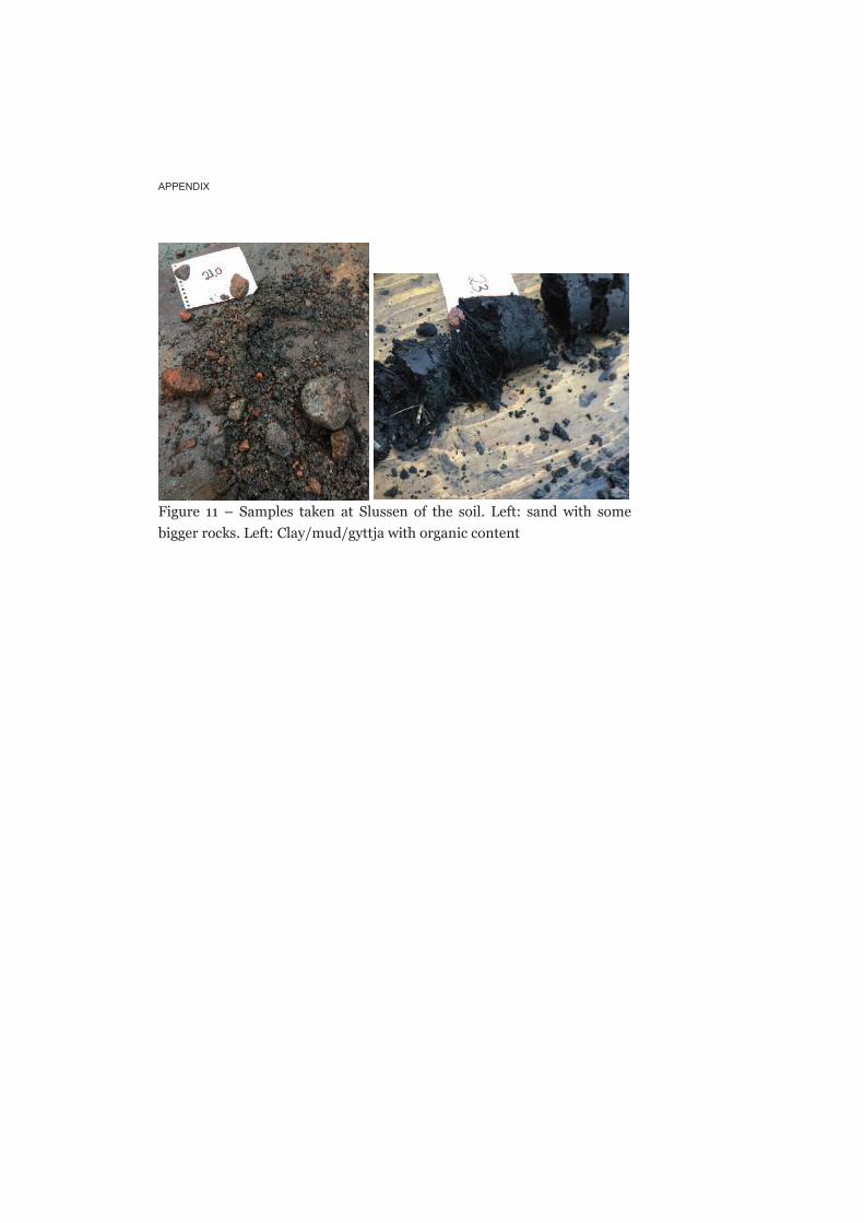
APPENDIX
Figure 11 – Samples taken at Slussen of the soil. Left: sand with some
bigger rocks. Left: Clay/mud/gyttja with organic content