Slip model of the 2015 Mw 7.8 Gorkha (Nepal) earthquake...

Slip model of the 2015 Mw 7.8 Gorkha (Nepal)

earthquake from inversions of ALOS-2 and GPS data

Kang Wang1, and Yuri Fialko

1

Corresponding author: Kang Wang, Institute of Geophysical and Planetary Physics, Scripps

of Institution of Oceanography, UC San Diego, La Jolla, CA, USA. ([email protected])

1Institute of Geophysical and Planetary

Physics, Scripps of Institution of

Oceanography, UC San Diego, La Jolla, CA,

USA.

This article has been accepted for publication and undergone full peer review but has not been throughthe copyediting, typesetting, pagination and proofreading process, which may lead to differences be-tween this version and the Version of Record. Please cite this article as doi: 10.1002/2015GL065201

c©2015 American Geophysical Union. All Rights Reserved.

We use surface deformation measurements including Interferometric Syn-

thetic Aperture Radar (InSAR) data acquired by the ALOS-2 mission of the

Japanese Aerospace Exploration Agency (JAXA) and Global Positioning Sys-

tem (GPS) data to invert for the fault geometry and coseismic slip distri-

bution of the 2015 Mw 7.8 Gorkha earthquake in Nepal. Assuming that the

ruptured fault connects to the surface trace of the of Main Frontal Thrust

fault (MFT) between 84.34◦E and 86.19◦E, the best-fitting model suggests

a dip angle of 7◦. The moment calculated from the slip model is 6.08×1020

Nm, corresponding to the moment magnitude of 7.79. The rupture of the 2015

Gorkha earthquake was dominated by thrust motion that was primarily con-

centrated in a 150-km long zone 50 to 100 km northward from the surface

trace of the Main Frontal Thrust (MFT), with maximum slip of ∼ 5.8 m at

a depth of ∼8 km. Data thus indicate that the 2015 Gorkha earthquake rup-

tured a deep part of the seismogenic zone, in contrast to the 1934 Bihar-Nepal

earthquake, which had ruptured a shallow part of the adjacent fault segment

to the East.


1. Introduction

The Mw 7.8 Gorkha (Nepal) earthquake occurred on April 25th, 2015 in the central

Himalaya, on a tectonic boundary resulted from the India-Eurasia collision. It caused more

than 8000 fatalities, and was the largest seismic event since the 1956 Assam-Tibet Nepal

Mw 8.6 earthquake along Himalayan arc [Bilham et al., 2001]. The CMT solution and

preliminary finite-fault inversions of seismic data suggested that the earthquake rupture

occurred along a NWW trending fault with a primarily thrust mechanism and a minor

component of dextral slip. Both the CMT solution and seismically determined finite-fault

models indicate that the dip angle of the fault is small (e.g. 7◦ in global CMT solution

[iris.edu, 2015] and 10◦ in the USGS determined finite-fault model [earthquakes.usgs.gov ,

2015]). Geologically, the most active structure along the Himalayan arc is the Main

Himalayan Thrust fault (MHT), which reaches the surface at Main Frontal Thrust fault

(MFT), and absorbs about 20 mm/yr of the India-Eurasia convergence in Nepal [Lave

and Avouac, 2000]. Analysis of GPS measurements before the Mw 7.8 Nepal earthquake

indicates that the MFT is locked from surface to a distance of approximately 100 km

down dip [Ader et al., 2012]. Most of the aftershocks of the 2015 event are located at least

30 km north of the MFT, suggesting that if the earthquake occurred along the MHT, it

may not have ruptured the shallow part of the fault. It has been suggested that the MFT

can be viewed as one of the splays of thrust faults rooting in a mid-crustal decollement

[e.g., Pandey et al., 1999; Avouac, 2003; Ader et al., 2012]. However, the geometry of

the decollement (in particular, its dip angle), is not well known. In this paper, we use

observations of surface deformation from Global Positioning System (GPS) and Synthetic


Aperture Radar (SAR) collected by ALOS-2 satellite of the Japanese Space Agency to

derive the slip distribution due to he 2015 Mw 7.8 Gorkha earthquake and constrain the

geometry of the earthquake rupture.

2. Data and Methods

The data used in the inversion include vector displacements measured at 13 GPS sta-

tions and Line-Of-Sight (LOS) displacements derived from Synthetic Aperture Radar

(SAR) data from 3 tracks of the ALOS-2 satellite (Figure 1). The raw GPS data are from

the network deployed by the Caltech Tectonics Observatory and processed by Advanced

Rapid Imaging and Analysis (ARIA) Center for Natural Hazards at JPL [Galetzka et al.,

2015]. Both horizontal and vertical components of the GPS displacements were used

in the inversion. ALOS-2 data were processed using GMTSAR [Lindsey et al., 2015].

The unwrapped InSAR phase was detrended by removing a linear ramp estimated from

far-field LOS displacements for each track to account for possible orbital errors and/or

ionosphere variations. InSAR data were down-sampled using a recursive algorithm that

enables denser sampling in areas of larger gradients in LOS displacements [Simons et al.,

2002; Fialko, 2004]. To avoid over-sampling in areas with large phase gradients due to

noise (atmospheric delays, decorrelation, unwrapping errors, etc.), our down-sampling of

the InSAR data was implemented iteratively using model predictions [e.g. Lohman and Si-

mons , 2005]. An initial slip model was estimated from inversion of coarsely sampled LOS

displacement maps. Synthetic interferograms were computed using the slip model, and

down-sampled using the quad-tree curvature-based algorithm. The bounding coordinates

of each resolution cell (bin) were then used to compute the average LOS displacements


from the observed interferograms. A new slip model was then derived from the updated

dataset. Usually, a few iterations are sufficient to achieve a solution that stops changing

with subsequent iterations. To avoid spurious shallow slip, a relatively dense sampling

around the fault trace was retained through all iterations (see Figure S1 of the supple-

mentary materials for the final down-sampling of the InSAR measurements in this study).

The radar incidence angles were computed by averaging the original values in respective

resolution cells.

Our kinematic inversions assumed that fault slip can be approximated by a superposition

of rectangular dislocations in a homogeneous elastic half-space [Okada, 1985]. The fault

geometry was constrained by the assumption that the rupture plane intersects the surface

along the MFT between 84.34◦E and 86.19◦E. The ∼ 185 km long and 160 km wide fault

was divided into patches which sizes gradually increase with depth to ensure a relatively

uniform model resolution [e.g. Fialko, 2004]. Each individual patch was allowed to have a

thrust and a right-lateral slip component of up to 10 m. Laplacian smoothing was applied

between adjacent fault patches to avoid abrupt variations in slip. We further regularized

the inversion problem by requiring no slip at the fault edges (except at the surface). We

determined the optimal values of smoothness of the model and relative weighting between

GPS and InSAR LOS data as described by Wang and Fialko [2014] (also see Figure S2

and Figure S3 of the supplementary materials).

The initial inversions were performed assuming a dip angle of 10◦. However, we found

that the best-fitting model failed to provide a good fit to data from the ascending and

descending tracks (T147 and T048) simultaneously, regardless of what model parameters


(e.g. degree of smoothing or relative weighting between GPS and InSAR data sets) were

chosen. We then allowed the dip angle to vary in the range of 1◦ - 15◦, and solved for

the slip distribution for each assumed geometry. For each run, we quantified the misfit

between the model and the data by calculating

χ2 =1

N

N∑i=1

(di − d′iσi

)2 (1)

where d and d′ represent vectors of observations and model predictions, respectively; σ

represents the corresponding uncertainty for each dataset (LOS displacements from 3

ALOS-2 tracks and horizontal displacements at 13 GPS sites); N is the length of the data

vector. Uncertainties in InSAR data were estimated by computing the variation of the

LOS displacements in the far field of each interferogram, where the deformation due to

earthquake is expected to be negligible. The estimated Root-Mean-Square (RMS) of the

LOS displacements in the far field are 2.3, 5.4 and 4.1 cm for track T047, T048 and T157,

respectively. We note that the variation estimated this way only provides a qualitative

measure of accuracy of the InSAR measurements, and does not reflect the uncertainty of

individual data points. The GPS uncertainties are computed as part of the GPS solutions,

and are mostly < 3 mm for horizontal components and < 1 cm for vertical component.

3. Results

We found that a model with a dip angle of 7◦ fits the LOS displacements from of all

3 ALOS-2 tracks as well as GPS data very well, with a low misfit of χ2 = 1.1561 (see

Figure S4 of the supplementary materials). The preferred coseismic slip model is shown in

Figure 2. The model is characterized by dominantly thrust slip, with minor contribution

of dextral component, concentrated in a relatively narrow (compared to the along-strike


rupture dimension) zone between ∼ 50 and ∼ 100 km along the down-dip direction. The

maximum slip is ∼ 5.8 m at a depth of ∼ 8 km with respect to sea level. The total

moment is 6.08 × 1020Nm, corresponding to a moment magnitude of Mw = 7.79, in

excellent agreement with the seismic moment [earthquakes.usgs.gov , 2015]. The slip on

the central part of the rupture seems to have extended further down-dip, compared to

both the eastern and western tips of the rupture that appear to taper to a width of 20-30

km (see Figures 2 and 5). Most of the aftershocks occurred along the eastern half of the

fault, around the patches of relatively large coseismic slip, including the Mw 7.3 aftershock

on May 12th, 2015 (magenta circle in Figure 2).

Figure 3 shows a comparison of the ALOS-2 data with predictions of the best-fitting

slip model (Figure 2). The model is able to reproduce InSAR measurements from all 3

tracks (Figure 3) as well as GPS measurements (Figure 1 and Figure S5). Interestingly,

a comparison with a coseismic interferogram made using Sentinel-1 data shows that the

latter under-predicts the amplitude of the LOS displacements by as much as 50% (Supple-

mentary Figure S7), likely due to a trade-off between the estimation of a burst alignment

and range changes intrinsic to the TOPS mode of Sentinel-1.

It was suggested that the MHT geometry involves two ramp-flats, with the top flat

lying at ∼ 5 to 10 km depth [Avouac, 2003]. To allow for listric (curved) fault geometry,

we performed another set of inversions in which the fault surface was parameterized as :

z = −2a

πarctan

y

b(2)

where z is the depth of the fault at a distance of y from the surface trace (i.e. MFT); a

and b are geometric parameters that were varied in the inversion. Specifically, a represents


the depth of the fault at infinite distance from the surface trace (corresponding to the

depth of the flat in the ramp-flat decollement system), while b controls the fault curvature

near the surface (corresponding to the geometry of the ramp in the ramp-flat decollement

system). A planar fault is particular case of equation (2), given sufficiently large b. Using

the same parameters for smoothness and relative weighting between datasets as before,

we inverted for the slip distribution on a curve fault described by equation (2) for a range

of values of a ∈ [1 : 1 : 30] km and b ∈ [1 : 10 : 300] km. The slip model yields the lowest

misfit of χ2curved = 1.0349 for a = 18 km and b = 81 km. This can be compared with

χ2planar = 1.1561 for the case of a planar fault, suggesting that a ramp-flat decollement

model is in better agreement with surface deformation data. The overall slip distribution

based on the curved fault is quite similar to that of a planar fault with a dip angle of

7◦ (Figure 2). The two models are very similar down to depth of 10 km, where most of

coseismic slip occurred (Figure 4). We also ran a suite of inversions in which we relaxed

the assumptions that the fault plane intersects the surface at the trace of MFT. In these

inversions, the fault strike was fixed at 285 ◦, and the fault was required to go through an

assumed hypocenter. Because the hypocenter depth is only approximately constrained by

seismic data, we allowed it to vary between 4 and 20 km. The fault dip was allowed to

vary between 1 to 15 degrees. The model misfits are shown in Figure S6, and the family

of fault geometries that fit the data equally well are shown by gray lines in Figure 4.

The respective slip distribution is quite similar to that of the planar fault that intersects

the surface at the location of MFT. The best-fitting geometries are close to sub-surface

geometries of the MHT suggested by previous studies [Avouac, 2003; Nabelek et al., 2009].


Somewhat shallower depths of the geodetic models compared to the inferred geometries of

the MHT (Figure4) might be attributed to the neglect of increases in elastic rigidity with

depth [e.g. Fialko, 2004]. However, we note that the seismically determined origin depth

is in better agreement with the best-fitting geodetic models than with the previously

suggested geometry of the MHT (Figure 4). The geodetically inferred dip angles are in

fact an upper bound, as model does not take into account surface topography. The average

slope due to topography across the MHT is 2 to 5 degrees (Figure 4), and a half-space

model is expected to bias the dip angle (measured with respect to the horizontal) by a

value of the order of the topographic slope. More sophisticated simulations that take

into account surface topography are needed to refine the slip model of the 2015 Gorkha

earthquake.

4. Discussion

Seismicity along the Himalayan arc is known to occur along a relatively narrow zone

which follows the front of high Himalaya, and tends to shut off underneath the higher

Himalaya (elevations higher than 3500 m, see the gray line in Figure 2) [e.g. Pandey

et al., 1995, 1999; Avouac, 2003]. The coseismic slip due to the 2015 Mw 7.8 Nepal

earthquake is also concentrated in a fairly narrow zone (between ∼ 50 and ∼ 100 km )

from the MFT at the deep end of the seismogenic zone. The extent of interseismic locking

at ∼ 100 km north of the MFT likely marks the brittle-ductile transition and changes in

rate dependence of friction due to the elevated pressure and temperature.

Our slip model shows that the 2015 rupture did not propagate into shallow part of the

MHT. Analysis of GPS measurements made before the earthquake indicates that the MHT


is locked from surface to a distance of approximately 100 km down dip [Ader et al., 2012].

Recent investigations of the Quaternary geomorphology along the MFT showed that at

least two great earthquakes had ruptured to the surface in Nepal in the past 1000 years

[Sapkota et al., 2013]. Particularly, the 1934 Bihar-Nepal M 8.2 earthquake ruptured a ∼

150 km-long segment of the MFT between 85.8◦ E and 87.3◦ E, immediately to the east of

the 2015 rupture (Figure 5). Unless the degree of seismic coupling varies along the fault

strike , the lack of shallow slip during the 2015 Gorkha earthquake implies future seismic

hazard, in particular because this part of the fault has been brought closer to failure by the

2015 earthquake. Observations of post-seismic deformation (in particular, the occurrence

of afterslip on the upper section of the MFT) will provide important constraints on the

degree of seismic coupling and seismic hazard on this part of this fault.

5. Conclusions

We used the surface displacement data provided by GPS and InSAR to model the

coseismic slip distribution and fault the geometry of the 2015Mw 7.8 Gorkha earthquake in

Nepal. Aftershocks of the 2015 event were mostly surrounding the areas of high coseismic

slip. The best-fitting model suggests a shallow dip angle of 7◦ for the MHT. The 2015

Gorkha earthquake ruptured the deep part of the seismogenic zone, with little or no slip

in the shallow part (within 50 km from the MFT). This is in contrast to the 1934 Bihar-

Nepal event, whose rupture had likely reached the surface, implying increased seismic

hazard on the fault section updip of the 2015 event.


Acknowledgments. We thank J.P Avouac, R. Bendick and the Associate Editor for

their thoughtful reviews. This work was funded by the National Science Foundation grant

EAR-1321932. Original ALOS-2 data are copyright by Japanese Aerospace Exploration

Agency (JAXA). The data and computer codes used in this paper are available form the

corresponding author.

References

Ader, T., J.-P. Avouac, J. Liu-Zeng, H. Lyon-Caen, L. Bollinger, J. Galetzka, J. Gen-

rich, M. Thomas, K. Chanard, S. N. Sapkota, S. Rajaure, P. Shrestha, L. Ding, and

M. Flouzat (2012), Convergence rate across the Nepal Himalaya and interseismic cou-

pling on the Main Himalayan Thrust: Implications for seismic hazard, Journal of Geo-

physical Research, 117 (B4), B04,403.

Avouac, J.-P. (2003), Mountain building, Erosion, and the seismic cycle in the Nepal

himalaya, Advances in Geophysics, Elsevier, 1–80.

Bilham, R., V. K. Gaur, and P. Molnar (2001), EARTHQUAKES: Himalayan Seismic

Hazard, 293 (5534), 1442–1444.

Chen, W.-P., and P. Molnar (1977), Seismic moments of major earthquakes and the

average rate of slip in central Asia, Journal of Geophysical Research, 82 (20), 2945–

2969.

earthquakes.usgs.gov (2015), Earthquake hazard program,

http://earthquake.usgs.gov/earthquakes/eventpage/us20002926#general summary,

(Accessed 30 June 2015).


Fialko, Y. (2004), Probing the mechanical properties of seismically active crust with

space geodesy: Study of the coseismic deformation due to the 1992 M w 7.3 Landers

(southern California) earthquake , Journal of Geophysical Research, 109 (B3).

Galetzka, J., D. Melgar, J. F. Genrich, J. Geng, S. Owen, E. O. Lindsey, X. Xu, Y. Bock,

J. P. Avouac, L. B. Adhikari, B. N. Upreti, B. Pratt-Sitaula, T. N. Bhattarai, B. P.

Sitaula, A. Moore, K. W. Hudnut, W. Szeliga, J. Normandeau, M. Fend, M. Flouzat,

L. Bollinger, P. Shrestha, B. Koirala, U. Gautam, M. Bhatterai, R. Gupta, T. Kandel,

C. Timsina, S. N. Sapkota, S. Rajaure, and N. Maharjan (2015), Slip pulse and reso-

nance of Kathmandu basin during the 2015 Mw 7.8 Gorkha earthquake, Nepal imaged

with geodesy., Science, pp. 1–9.

iris.edu (2015), Moment Tensor for MW 7.9 (GCMT) NEPAL,

http://ds.iris.edu/spud/momenttensor/9925741, (Accessed 30 June 2015).

Lave, J., and J.-P. Avouac (2000), Active folding of fluvial terraces across the siwaliks

hills, himalayas of central nepal, Journal of Geophysical Research, 105 (B3), 5735–5770.

Lindsey, E., R. Natsuaki, X. Xu, M. Shimada, M. Hashimoto, and D. Sandwell

(2015), Nepal earthquake: Line of Sight Deformation from ALOS-2 Interferometry,

http://topex.ucsd.edu/nepal/ , (Accessed 30 June 2015).

Lohman, R. B., and M. Simons (2005), Some thoughts on the use of InSAR data to

constrain models of surface deformation: Noise structure and data downsampling, Geo-

chemistry, Geophysics, Geosystems, 6 (1), Q01,007.

Nabelek, J., G. Hetenyi, J. Vergne, S. Sapkota, B. Kafle, M. Jiang, H. Su, J. Chen, B.-S.

Huang, and H.-C. Team (2009), Underplating in the Himalaya-Tibet Collision Zone


Revealed by the Hi-CLIMB Experiment, Science, 325 (5946), 1371–1374.

Okada, Y. (1985), Surface deformation due to shear and tensile faults in a half-space,

Bulletin of the Seismological Society of America, 75 (4), 1135–1154.

Pandey, M. R., R. P. Tandukar, J. P. Avouac, J. Lave, and J. P. Massot (1995), Interseis-

mic strain accumulation on the Himalayan crustal ramp (Nepal), Geophysical Research

Letters, 22 (7), 751–754.

Pandey, M. R., R. P. Tandukar, J. P. Avouac, J. Vergne, and T. Heritier (1999), Seismo-

tectonics of the Nepal Himalaya from a local seismic network, Journal of Asian Earth

Sciences, 17 (5-6), 703–712.

Sapkota, S. N., L. Bollinger, Y. Klinger, and P. Tapponnier (2013), Primary surface

ruptures of the great Himalayan earthquakes in 1934 and 1255, Nature Geoscience,

6 (2), 152–152.

Simons, M., Y. Fialko, and L. Rivera (2002), Coseismic Deformation from the 1999 Mw

7.1 Hector Mine, California, Earthquake as Inferred from InSAR and GPS Observations,

Bulletin of the Seismological Society of America, 92 (4), 1390–1402.

Wang, K., and Y. Fialko (2014), Space geodetic observations and models of postseismic

deformation due to the 2005 M7.6 Kashmir (Pakistan) earthquake, Journal of Geophys-

ical Research: Solid Earth, 119 (9), 7306–7318.


83˚

83˚

84˚

84˚

85˚

85˚

86˚

86˚

87˚

87˚

88˚

88˚

89˚

89˚

26˚ 26˚

27˚ 27˚

28˚ 28˚

29˚ 29˚

30˚ 30˚

83˚

83˚

84˚

84˚

85˚

85˚

86˚

86˚

87˚

87˚

88˚

88˚

89˚

89˚

26˚ 26˚

27˚ 27˚

28˚ 28˚

29˚ 29˚

30˚ 30˚

0 100

km

MainFrontal

~20 mm/yr

Thrust

T048

T157

T047 Everest

100 cm ObservationModel0

2000

4000

6000

8000m

INDIA

CHINA

~ 40

mm

/yr

Figure 1. Tectonic setting of the 25 April, 2015 Mw 7.8 Nepal earthquake. Thick black

line represents the surface trace of the Main Frontal Thrust (MFT) [Ader et al., 2012]. The

redstar denotes the epicenter [earthquakes.usgs.gov , 2015], and the beachball denotes the Cen-

troid Moment Tensor [iris.edu, 2015] of the Mw 7.8 mainshock. White boxes show the coverage

of ALOS-2 data (ascending track T157, descending track T048, and 5th sub-swath of descend-

ing track T047). Blue and red arrows represent the observed and modeled horizontal surface

displacements at GPS sites (magenta triangles)


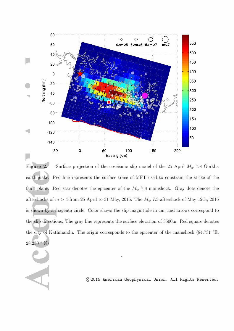
Figure 2. Surface projection of the coseismic slip model of the 25 April Mw 7.8 Gorkha

earthquake. Red line represents the surface trace of MFT used to constrain the strike of the

fault plane. Red star denotes the epicenter of the Mw 7.8 mainshock. Gray dots denote the

aftershocks of m > 4 from 25 April to 31 May, 2015. The Mw 7.3 aftershock of May 12th, 2015

is shown by a magenta circle. Color shows the slip magnitude in cm, and arrows correspond to

the slip directions. The gray line represents the surface elevation of 3500m. Red square denotes

the city of Kathmandu. The origin corresponds to the epicenter of the mainshock (84.731 ◦E,

28.230 ◦ N)

.


Figure 3. Comparison of observed and modeled LOS displacements from 3 ALOS-2 tracks.

The forward calculation is based on a model assuming a planar fault with the dip angle of 7◦ that

intersects the surface at the trace of MFT (Figure 2). The top (a-c), middle (d-e) and bottom

(g-i) panels are observations, model predictions and residuals, respectively. Note the differences

in color scales between the data/models and the residuals. Sub-titles denote the track numbers

and SAR acquisition dates (in parentheses; all in year 2015).


0 20 40 60 80 100 120 140 160−25

−20

−15

−10

−5

0

Distance from MFT (km)

Dep

th (

km)

Nabelek et al. (2009)

Avouac (2003)

0

2

4

6

8

Ele

vatio

n (k

m)

0

5

10

15

20

25

% o

f mom

ent r

elea

se

Plane (Dip=7°)Plane (Dip=4°)ARCTAN (a=18km and b=81km)

Figure 4. Comparison of slip models assuming planar and curved fault geometry. (a) moment

release and topography along dip direction. The shaded gray area shows the elevation variations

along the direction normal to the average strike of MFT ( 285◦) as marked by red line in Figure

2. The blue red and green lines show the percentages of moment release as a function of distance

from MFT for the three best-fitting fault geometries:. (b) geometries of the fault models at depth

(blue for planar fault of dip angle of 7 ◦ that intersects the surface at MFT, green for curved

fault approximated by an arctan function, red for planar fault with dip angle of 4 ◦ ). Thin

gray lines represent the geometries of planar faults yielding low misfits (see Figure S6). The red

circle with error bars represents the hypocentral depth of the mainshock. The dashed black and

magenta lines denote the geometries of MHT inferred by Nabelek et al. [2009] and Avouac [2003]

, respectively.


84˚

84˚

85˚

85˚

86˚

86˚

87˚

87˚

88˚

88˚

27˚ 27˚

28˚ 28˚

84˚

84˚

85˚

85˚

86˚

86˚

87˚

87˚

88˚

88˚

27˚ 27˚

28˚ 28˚

0 100

km

MainFrontal

Thrust

84˚

84˚

85˚

85˚

86˚

86˚

87˚

87˚

88˚

88˚

27˚ 27˚

28˚ 28˚

100 200 300 400 500 600cm

2015 M7.8

VIII

1934

Figure 5. Spatial relationship between the 2015 Mw 7.8 Gorkha earthquake and the 1934 Mw

8.6 Bihar-Nepal earthquake. Color represents the coseismic slip of the 2015 event. Yellow dots

denote the aftershocks of the 2015 event from April 25, 2015 to May 31 2015. Lightgreen dots

denote the background seismicity from 1995 to 2002 [Ader et al., 2012]. Red solid and dashed

lines represent the inferred rupture segment and the isoseismal intensity of VIII of the 1934

Bihar-Nepal earthquake, respectively [Sapkota et al., 2013]. Magenta star denotes the relocated

epicenter of the 1934 event [Chen and Molnar , 1977].

.


Slip model of the 2015 Mw 7.8 Gorkha (Nepal) earthquake...

Documents

Transcript of Slip model of the 2015 Mw 7.8 Gorkha (Nepal) earthquake...