Sliding Mode Control of the X-33 With an Engine Failure ... · PDF fileSliding Mode Control of...

AIAA-O0-####

Sliding Mode Control of the X-33 With an Engine Failure

Yuri B. Shtessel + , Charles E. Hall _

Abstract

Ascent flight control of the X-33 is performed using two XRS-2200 linear aerospike engines, in addition to

aerosurfaces. The baseline control algorithms are PID with gain scheduling. Flight control using an innovative

method, Sliding Mode Control. is presented lbr nominal and engine failed modes of flight. An easy to implement,

robust controller, requiring no reconfiguration or gain scheduling is demonstrated through high fidelity flight

simulations. The proposed sliding mode controller utilizes a two-loop structure and provides robust, de-coupled

tracking of both orientation angle command profiles and angular rate command profiles in the presence of engine

failure, bounded external disturbances (wind gusts) and uncertain matrix of inertia. Sliding mode control causes the

angular rate and orientation angle tracking error dynamics to be constrained to linear, de-coupled, homogeneous, andvector valued differential equations with desired eigenvalues. Conditions that restrict engine failures to robustness

domain of the sliding mode controller are derived. Overall stability of a two-loop flight control system is assessed.

Simulation results show that the designed controller provides robust, accurate, de-coupled tracking of the orientation

angle command profiles in the presence of external disturbances and vehicle inertia uncertainties, as well as the

single engine failed case. The designed robust controller will significantly reduce the time and cost associated with

fixing new trajectory profiles or orbits, with new payloads, and with modified vehicles.

I. Introduction

Attitude control for the X-33 depends primarily

on its two linear aerospike engines lbr ascent flight.Aerosurfaces are effective only during regions of

flight with sufficient dynamic pressure, therefore theengines must pro_ lde all attitude control at liftoff, and

the majority of the control at high altitudes. Ascent is

quite demanding of the Ascent Flight Control System,

or AFCS, due to the many trajectory requirements,

operating constraints for the engines and

areosurfaces, and the presence of high winds at the

launch site. A thorough expose of the baseline X-33

attitude control system and description of the flight

profile may be found in [13]. A description of theoperation and control of the XRS-2200 linear

aerospike engine may also be found in this reference.

The baseline AFCS, employs a variable structure

PID control law [ 12] with gain scheduling. This

requires four gains per channel that are looked upfrom a table as a function of relative velocity.

Depending on the flight trajectory, each gain table

can have as many as 25 values, so potentially 300

gain values must be stored in the on board computerfor nominal flight. In case of an engine failure, or

Power Pack Out (PPO) alternate sets of gain tables

are used, depending on the flight time when thefailure occurred. Provisions are made for 25 possible

PPO times, or 25 sets of PID tables. This amounts to

another 7500 values to be stored, or a total of 7800

values to provide gains for the nominal and enginefailed cases.

* Associate Professor, Electrical and Computer Engineering Dept., University of Alabama, Huntsville, AI.

* Aerospace Engineer, Control Systems Group, NASA, MSFC

Copyright © 2000 by the American Institute of Aeronautics and Astronautics, Inc. No copyright is asserted in theUnited States under Title 17, U.S. Code. The U.S. government has royalty-free license to exercise all rights under the

copyright claimed herein for Governmental Purposes. All other rights are reserved under the copyright owner.

1

American Institute of Aeronautics and Astronautics

https://ntrs.nasa.gov/search.jsp?R=20000072424 2018-05-13T12:34:25+00:00Z

O

X-33 aerospike engine test firing at Stennis SpaceCenter.

The reason for so many gain tables is because thecontrol system design relies on linear analysis and

perturbation theory at specific design points along thetrajectory. This method is well established and has

been used in many launch vehicle control system

designs, therefore well understood and reliable tools

and design methods may be used. Robust control is

ensured as long as the vehicle performance and

operating conditions are relatively close to the design

points. For the X-33, the vehicle performance and

operating conditions as a function of relative velocity

is verv different bet_veen the first flight trajectory and

the second. These design point parameters are

drastically different with a failed engine, as can be

seen in figures 1 and 2. Therefore, alternate tables areneeded for robust control to fly different trajectories,

or to accommodate an engine failure at various times.

35O

- ! : : :

_-" _"F _,...................... _ .......... I _ Second FLight _-

300r /_/ \ [ _ OOO at 60 Seconds Ii

250 ! _i_ : :

200F,/'i ..........\ ...................

;.................i.....100 ........

0 _ L , , , t , . t , , ,

0 2000 4000 6000 8000 1 106

Rihltlve Velocity (fUse(;)

Figure 1: Dynamic pressure vs. relative velocity.

.o

w

_-_ ! ___ | _ Second FLight

4105 _; _'i ............ L --*_'_-- PFO at 60 Seconds

31o' ........

2td

11_ ......L

0 2_0 4_0 6_0

1: 1

8000 lo"

Relative Velocity (ft/sec)

Figure 2: Thrust vs. relative velocity.

Flight control of the X-33 technologydemonstration sub orbital launch vehicle in ascent

mode involves attitude maneuvering through a wide

range of flight conditions, wind disturbances anduncertainties of the X-33 mathematical model,

including uncertain matrix of inertia and an engine

failure. A robust flight control algorithm that wouldaccommodate different trajectories and an engine

failure without gain scheduling would be an

improvement over the X-33 current flight controltechnology. Sliding Mode Controller (SMC) is an

attractive robust control algorithm for the X-33 ascent

designs because of its inherent insensitivity and

robustness to plant uncertainties and externaldisturbances 13, Such a controller would drastically

decrease the amount of time spent in pre-flight

analysis, thus reducing cost.

A SMC design consists of two major steps: (1) a

sliding surface is designed such that the systemmotion on this surface exhibits desired behavior in

the presence of plant uncertainties and disturbances;and (2) a control function is designed that causes the

system state to reach the sliding surface in finite timeand guarantees system motion in this surface

thereafter. The system's motion on the sliding surface

is called sliding mode. Strict enforcement of the

sliding mode typically leads to discontinuous controlfunctions and possible control chattering effects 4.

Control chattering is typically an unwanted effect that

is easily eliminated by continuous approximations ofdiscontinuous control functions 4'5, or by continuous

SMC designs 6.

2


AnexampleoftheapplicationofSMCisshowninthespacecraftattitudecontrol_orkperformedbvDwyeretal. Thisworkutilizesthenaturaltime-scaleseparation,whichexistsinthesxstemdynamicsofmanyaerospacecontrolproblemss,

TheX-33SMCarchitecture,whichisdevelopedinthepaper°,isatwo-loopstructurethatincorporatesbacksteppingtechniquesm.Intheouter loop, the

kinematics equation of angular motion is used x_ith

the outer loop SMC to generate the angular rate

profiles as virtual control inputs to the inner loop. In

the inner loop, a suitable inner loop SMC is designedso that the commanded angular rate profiles are

tracked. The inner loop SMC produces roll, pitch and

yaw torque commands, which are optimally allocated

into end-effector deflection commands. Multiple time

scaling (multiple-scale) is defined as the time-

constant separation between the two loops. That is,

the inner loop compensated dynamics is designed to

be faster than the outer loop dynamics. The resulting

multiple-scale two-loop SMC, with optimal torque

allocation, causes the angular rate and the Euler angle

tracking errors to be constrained to linear de-coupled

homogeneous vector valued differential equations

with desired eigenvalues placement.

Simulation results are presented that demonstrate

the SMC's effectiveness in causing the X-33

technology demonstration vehicle, operating in ascent

mode, to robustly follow the desired profiles. The

resulting design controls large attitude maneuvers

through a _ide range of flight conditions, provides

highly accurate tracking of guidance trajectories, andexhibits robustness to external disturbances,

parametric uncertainties, and an engine failure.

Equations of the X-33 dynamics

particular payloads from a nominal one,

_o=[p q r] r is the angular rate vector,

T={L,M,N} r is the control torque vector,

d = {L,,M,,,N a }r is the external disturbance

torque vector. The matrix -('2 is given by:

0 - _ _2

_ 0 - _,- _: _l 0

(2)

The X-33 orientation dynamics are described by

the kinematics equation on the body axes

)_ = R(y)w, (3)

where

R(y) =

y = [rp

1 tan0sin¢ tan0cos_0

0 cos cp - sin _0

0 sinq9 cos_0cos 0 cos 0

0 _]r

(4)

The equations of the X-33 translationalmotion are available as well 9 but not presented in the

paper, because they do not effect the orientation angle

controller design. However, these equations are used

during 6DOF high fidelity simulations to assess

performance of the designed sliding mode controller.

The control torque T is generated by the

aerodynamic surfaces and rocket engines. This is

described by the equation

The dynamic equations of rotational motion of the

X-33 rigid-body are given by the Euler equation in

the body frame

(Jo + AJ_ = -_(Jo + M_+ T +d , (1)

T = D(.)S, (5)

where D(.)e R 3x" is a sensitivity matrix calculated

on the basis of table lookup data, _ E R" is the

vector of aerodynamic surface deflections and

differential throttles of the rocket engines.

where J0 E R3X3 is the nominal inertia matrix,

AJ E R 3x3 is an uncertain part of the inertia matrix,

caused by fuel consumption and variations of

Electromechanical actuators deflect the

aerodynamic surfaces (aerosurfaces), and thrust-

3


vector-controlvalvesthatthrottletherocketengines.executingthefollowingcommands

_5 = D"(.)T. 15a)

where a control allocation matrix D o (.) that meets a

pseudo-inverse condition D(.)D(.)_ = I can be

calculated as follows:

D' (.) = D(.)v [D(.)D(.)a- ]-l (5b)

The actuator dynamics are assumed to be much

faster than the dynamics of the compensated X-33

flight control system that permits to assume _ --- _c"

The "'fast" actuator dynamics are neglected at the

stage of the controller design. Thev will be usedduring simulations to validate the designed controller.

Taking into account possible engine failures, the

actual sensitivity matrix must be rewritten. This is

D,,,., (.) = D(.) + AD(.), (5c)

where AD(.) is an uncertain component of the

sensitivity matrix due to possible engine failures,

while the allocation matrix D#(.) is still calculated

on the basis of the nominal sensitivity matrix in

accordance with eq. (5b). Taking into account eqs.

(5a) and (5c) the control torque in eq. (5) must berecalculated as

T,.= (D(.)+ AD(.))6, (5d)

where T,. stands for the actual control torque

generated by the deflections _..

Substituting eq. (5a) into the eq. (5d) we obtained

a final expression for the actual control torque

T c = (I + E)T, (5e)

where E = ,Z,,D(.)D _

Problem Formulation

The problem formulation is to determine the

actuator deflection commands d) such that the

commanded Euler angle profiles

y, = [q_ O. _,.]r are robustly followed in the

presence of bounded disturbance torque d, the X-33

inertia variations AJ and engine failures that are

described by the uncertain matrix AD(.).

The control problem for the X-33 in ascent orlaunch mode is to determine the control torque input

command vector T in the given state variable

equations

(Jo + AJ)°):-fa(Jo + AJ)to + (I + E)T +d,

(7a)

?' = R(y)to, (7b)

y = y. (7c)

where E = ._D(.)D _, such that the output vector y

asymptotically tracks a command orientation angle

profile y,. = y,,. That is,

,--,®lim.v,,.(t) - y, (t) = 0 Vi = 1,3. (8)

The desired X-33 performance criteria is to

robustly track both the commanded Euler angle

guidance profiles Yc and the real-time generated

angular rate profiles O)c , such that the motion for

each quantity is described by a linear, de-coupled,

and homogeneous vector valued differential equations

with given eigenvalues.

Sliding Mode Controller Design

Tracking of the commanded Euler angles

guidance profile Yc (the primary objective) is

achieved through a two loop SMC smacture 9. The

cascade structure of the system in eq. (7) and theinherent two time scale nature of the X-33 flight

control problem are exploited for design of a two

loop flight control system using continuous SMCs in

the inner and outer loops. The outer loop SMC

4


providesangularratecommandsCOtotheinnerloop.TheinnerloopSMCprovidesrobustde-coupledtrackingofangularrates_:0.Together,theinnerandouterloopSMCsformatxvoloopflightcontrolsystemthatachievesde-coupledasymptotictrackingofthecommandangleguidanceprofiley,.Similarstructurev,asdevelopedforanaircraftcontrolsystemusingadynamicreversionalgorithm.which,ho_vever,doesnotexhibitver,vrobustbehavtor.

Outer Loop Sliding Mode Controller Design

The outer loop SMC takes the X-33 angular

rate vector to as a virtual control to,. and uses the

kinematics eq. (7b) to compensate the Euler angle

tracking dynamics. The motion of the outer loop

compensated tracking error dynamics, with desired

bandwidth, is constrained (by proper control action)

to a sliding surface of the form

cr=y_+K_iydr, o-_R 3 , (9)0

where Y, = gc - Y and

K_ =diag{k_,}, Kte R 3×3. The gain matrix

K_ is chosen so that the output tracking error },',

exhibits a desired linear asymptotic behavior on the

sliding surface ( Cr = 0 ).

The objective of the outer loop SMC is to

generate the commanded angular rate vector to.

(which is passed to the inner loop SMC) necessary tocause the vehicle's trajectory to track the commanded

Euler angles guidance profile Yc • In other words,

the virtual control law (Oc is designed to provide

asymptotic convergence (with finite reaching time) of

the system's eq. (7b) trajectory to the sliding surface

O" = 0. Dynamics of the sliding surface in eq. (9) aredescribed a_

O" = Yc - R(y)toc + KI_/e . (10)

The outer loop SMC design is initiated by

choosing a candidate Lyapunov function of the form

V 1 re=-t7 >0,2

(11)

whose derivative is shown as

= o'T{7 = o'T[y, -- R(ylto. + Kty,,]. (12)

To ensure asymptotic stability' of the origin of the

system in eq. (10). the following derivative inequalityof the candidate Lyapunov function is enforced TM

(/= -per r SIGN(or) = -py lcr, l, p > o.i=1

(13)

Considering eq. (13), the required angular rate

command toc to ensure asymptotic stability is

defined as

to. = R-' (y)[?_ + K0, , ] + R -_ (y)pSlGN(tr)

(14)

where

SIGN(or) = [sign(ty_ ), sign(or: ), sign(or 3 )_,

and p > 0.

The sliding surface shown in eq. (9) will reachzero in a finite time _a defined as

t r = max It:r'(0)1

te[I,3l p

(15)

where p >0, and t, is the design parameter

describing the sliding surface reaching time. The

value of p is calculated using eq. (15).

The angular rate command profile in eq. (14) isdiscontinuous; as a result, the control actuation will

chatter during system operation on the sliding surface

eq. (9). Mechanically and electrically, this chatteringis an unwanted effect. Moreover, a discontinuous

profile cannot be accurately tracked in the inner loop.

To solve this problem, the discontinuous term

(SIGN(or) ) in eq. (14) is replaced by the high-gain

linear term

5


' T

KoO'= o" l 0": 0" 3

f_ F, 6 3

{÷I -K 0=diag V6 >071.3

(16)

x_here 6 > 0 '7'1.3 define the slopes of the

lineanzed tuncnon '.

After substitution of eqs. ( 16_ and 114) into eq.

t 101. the sliding surface dynamics are of the form

a = -PKoa. (17)

Eq. (17) is globally asymptotically stable, since

19 > 0 and K o is positive definite, and the

equilibrium Cr = 0 will be reached asymptotically.

Moreover, in a close vicinity of G = O, Vi = 1,3,

the tracking error )/e will exhibit de-coupled motion

in accordance with eq. (9).

Inner Loop Sliding Mode Controller Design

The purpose of the inner loop SMC is to

generate the vehicle torque command vector Tnecessary to track the given commanded angular rate

profile fo. In addition to solving the inner loop

tracking problem defined as

limifo - (t) =0, Vi 1.3.,-.- ,,(t) w, = (18)

SMC causes the system to exhibit linear decoupled

motion in sliding mode.

The motion of the inner loop compensated

dynamics, with desired bandwidth, is constrained (by

proper control action) to a sliding surface of the form

t

s=fo +K:f%dv, s_R:',0

(19)

where fOe = fOc - 09 and

K, =diag{kz}, K 2 _ R 3×3. The angular rate

tracking error fo exhibits a desired linear asymptotic

behavior while operating on the sliding surface

( s = 0 ) and with proper choice of K 2. The inner

loop sliding mode dynamics in eq. (19) are designed

faster than the outer-loop sliding mode dynamics in

eq. (9) in order to preserve sufficient time scale

separation between the loops.

The command torque T is designed to provide

asymptotic convergence (with finite reaching time) of

the system's eq. (7a) trajectory to the sliding surface

s = 0. Dynamics of the sliding surface eq. (19) aredescribed as follows:

g':6L +(J0 + zkJ)-'Q(J0 + &J)w-

(J0 + &J)-' (I + E)T,. -(Jo + _J)-'d + K_,fo

(20)

Assuming the matrix I + E is positive definite, thatrt

be achieved if £ E j < 1 Vi = l,n, andcan

j=l

considering a fact that the inertia matrix J0 + AJ is

positive definite, the inner loop SMC design is

initiated by choosing the candidate Lyapunovfunction of the form

v=lsT(I+E)-'(Jo +AJ)s>O, (21)2

whose derivative is shown as

I)={srI(I+E)-t[AJ-E(I+E)-'_+_

(I+E)-'(J o+AJ)o) +(I+E)-'(J o+AJ)K2w +

(I + E)-t_(J 0 + AJ)m- Wc - (I + E)-td }

(22)

To ensure asymptotic stability of the origin of the

system eq. (20), the following derivative of the

Lyapunov function candidate is enforced t4

3

(z <__rls r SIGN(s) = -7"/Z a,[, r/> O.i=1

(23)

Further, the sliding surface eq. (19) will reach zero in

a finite time _4 defined by

z r _<max' 'IS' (0)1, (24)

ie[l,31 T]

6


where/7 > 0, and _'r is the design parameter

describing the sliding surface reaching time. The

value of /7 is calculated using inequality (24).

Considering inequality 123). the required torque

command T to ensure asymptotic stability is definedas

T : JoCb * JoK.w< + D.J0w + 1 Ms +- 9

_SIGN(s)

(25t

m

where M = diag_u }. It, > 0 Vi = 1.3. One

should note that the SMC eq. (25) is independent of

uncertainties AJ. A J, E, E and disturbances d.

Substituting eq. (25) into eq. (22) yields

isf E-/5 s, - r M-(I+E)-I s+= 2 E(I + E)-'

sr [((I + E)-'(Jo +AJ)-Jo_ ' +

((I + E)-I (Jo + AJ)- Jo )K_,oJ< +

((I + E)-' ff2(J o + AJ)- D_Jo )o- (I + E)-'d ]

(26)

Selecting the mamx

M = diag,: }, #, > 0 Vi = 1.3 to diagonally

dominate the matrix (I + E)-l(&i-E(I + E) -l)

we ca find a positive definite matrix Q such that

srQs > s r {M-(I + E)-' [Aj - E(I + E) -I 1t_.

(26a)

Assuming

I[((I+E)-'(Jo+zxJ)-Jo)a,,.],l<a,,Ib÷E)-'(Jo+zXJ)-Jo)K=°',],I<b,,

I[((l+I[(I+E)-'d],l<L, (27)

we can re_,Tite eq. (26) as follows:

3 isl)<-_[](/5-a-b,-c,-L,)s,--_ rQs<

3

-?_-a,-b,-c,- L,)l',lt=l

(28)

Inequality (28) is rewritten to enforce inequality (23)

after selecting t./ > ,,_. This is.

3 3

v _<-Z(_-a,-b,-c,- L,)ls,-<-/7El,,i=1 l=l

(29)

The value of parameter /_ is identified in accordance

with inequality (29) as follows:

/5 > a, +b, +c, +L, +/7

(30)

Remark. The constants a,, b i, c,, L, Vi = 1.3. are

derived by estimating the upper bounds of

inequalities (27) within a reasonable flight domain.

To avoid chattering, the SMC eq. (25) is

implemented in a continuous form

T = J0cb. + Jo K,_cO + .c2J0co + 1 Ms + pSAT(Fs)2

, (31)

where

ia,{F= (=,J

S 1 S 2 S 3, sat --, satSAT(Fs) = sat-z--

1, if s, > (,Si Si

sat _ = --(i f , if Is, <(,

L-l, Cs, <-¢,

(32)

7


bythefirstthreeequationsineqs.(36)areboundedwithboundarywidthsproportionalto (: Vi = 1,3.

Design and Simulation of the X-33 ControlSystem in Ascent Mode

The X-33 technology demonstration vehicle

controller design is considered in ascent mode. The

6DOF high fidelity mathematical model includes the

control deflection vector _ E R _ that consists of

the tbllowing components: _l and (3, are

deflections of the right and left flaps, _3 and _._ are

deflections of the right and left inboard elevons, _5

and (36 are deflections of the right and left outboard

elevons; _7 and (38 are deflections of the right and

left rudders; _9, _lo, and _ll are pitch, roll and

yaw differential throttles (in % of power level) of the

aerospike rocket engine. Flight guidance tables for

the Euler angle command profiles },'. are used. High

fidelity quantized sensor mathematical models with

0.02 s time delay as well as realistic table look up

wind gust profiles that create a disturbance torque arealso used.

The command profiles O) and T are generated

by the outer and inner loop SMCs in eqs. (14), (16)

and (31). The deflection command vector _. is

calculated in eq. (6) and executed by the actuators,

whose dynamics are contained in high fidelity modelsused in the simulations.

The outer loop continuous SMC is designed in

accordance with eqs. (9), (14) and (16). The

following outer loop SMC parameters are chosen:

p=l,

i.3 0 0 ]K l = 0.3 0 ,

0 0.3J

0.8 0 0]

K0=/0 0.9 0 l,

[_0 0 0.9_1

(42)

where the matrix KI provides a 0.3 rad/s given

bandwidth for the compensated outer loop. The inner

loop continuous SMC is designed in accordance with

eqs. (19). (30) and (31). The following inner loop

SMC parameters are chosen:

1.5.106 0 0

/9 = 0 1.8-106 0

0 0 2.0"106

l l'0o o ]K.=0 1.00 ,

0 0 1.0

_, = 1.0 Vi = 1.3. (43)

N • r?l,

where the matrix K, provides a 1.0rad/sec

given bandwidth for the compensated inner loop, and

M=0.

A high fidelity six degree-of-freedom flight

simulation was used to test the performance of the

SMC for nominal flight and with an engine failure,PPO at seconds. The simulation, called Maveric

(Marshall Aerospace Vehicle Representation In C), is

the same one used for X-33 flight analyses, modified

to accept the SMC. The same flex filters used in thebaseline controller were used in the SMC. Maveric

employs detailed, non-linear models for the two

aerospike engines, electro-mechanical actuators for

the aerosurfaces with associated linkages, and Inertial

Navigation Unit (INU). All flight software is

emulated, and data latency from unmodeled

computations in the INU and in the data bus aresimulated. Forces and torques from propellant slosh

is included, as well as a mean annual wind profile atEdwards Air Force Base, where the X-33 will be

launched.

Should one of the X-33's two engines fail, they

are capable of re-configuring such that propellantflow can be diverted from the remaining functional

engine, to the thrust cells of the failed engine. This is

called Power Pack Out (PPO) mode. When one

engine fails, the Gas Generator and turbo pumps in

the failed engine are shut down. Then, two inter-

engine isolation valves, one for fuel and the other for

oxidizer, are opened allowing propellant flow from

the functional engine to the thrust cells in the failedengine. In this way, both engines can provide thrust

and thrust vector control as before, only at half the

8


nominallevel.ThePPOmodewassimulatedat secinflight.The sensed orientation angle tracking errors

are shown in fig. 15.

The 6DOF time simulation results for the

first flight guidance trajectory are presented in

figures 3 - 17. Figures 1 - 3 show overall tracking

performance of the Euler angle guidance profiles in

the outer loop, which is obviously decoupled and

very accurate. Figure 4 confirms existence of a

sliding mode in the outer loop, since the Euler angle

tracking happens in a close-to-zero vicinity of the

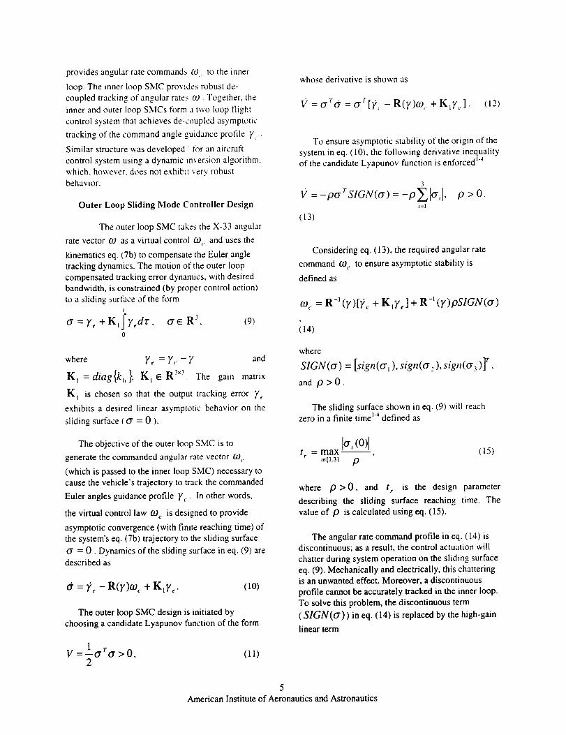
outer loop sliding surfaces. Figures 5-7 show

reasonably accurate tracking the angular rates

command profiles in the inner loop. A piece-wise

constant shape of the sensed rate profiles that are

displayed in figures 6 and 7 is caused by quantization

of sensored data from gyros. It's also worth noticing

that in figure 8 the sliding surface 2 ( s_, ) deviates

significantly from zero still being limited by the

szl < _'z = 1.0. This deviation isboundary layer:

due to a large disturbance in the pitch channel and

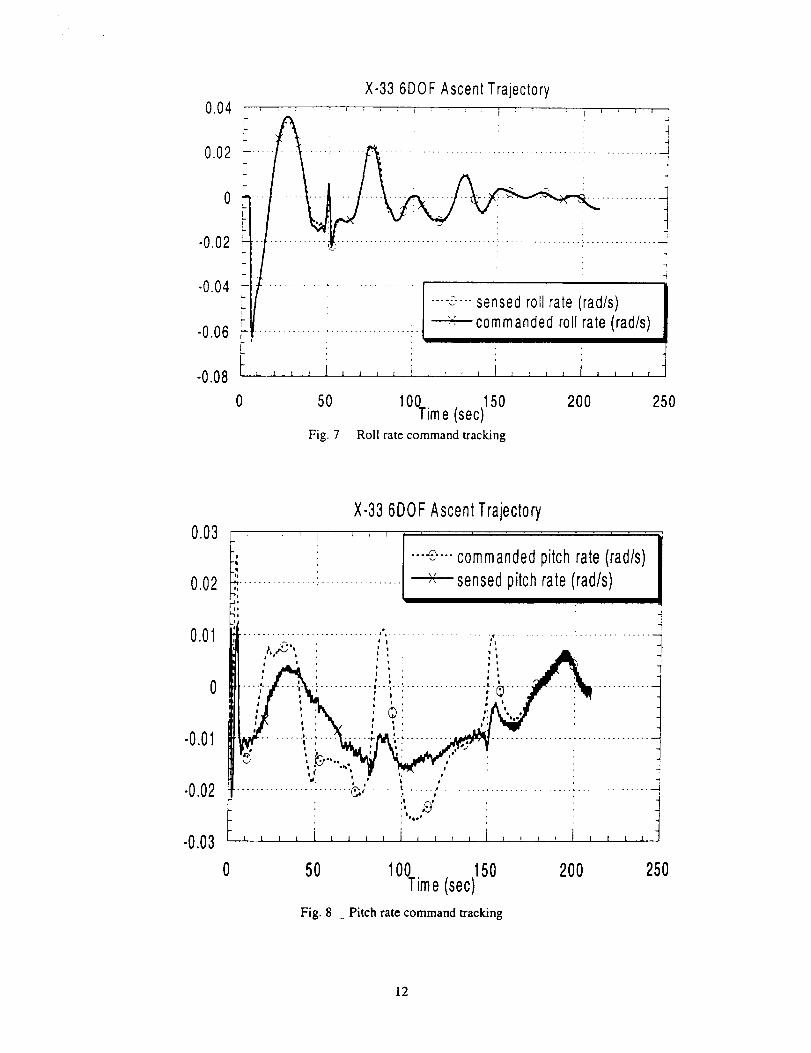
can be estimated by eq. (36). Figure 9 demonstrates

torque command profiles T. These commands are

allocated into actuator deflection s _. and rocket

engine throttle commands executed by the actuators.

Figures 10-14 demonstrate corresponding enginedifferential throttles and sensed deflections of the

aerodynamic surfaces that are far from saturation.

Conclusions

Employing a time scaling concept in the inner

(angular rates) and outer (orientation angles) loops, a

new two-loop continuous sliding mode controller

was designed for the X-33. This sliding mode

controller provides de-coupled performance in the

inner and outer loops in presence of bounded external

disturbances and plant uncertainties. Stability of the

two-loop control system is analyzed. A control

allocation matrix is designed that optimally

distributes the roll, pitch, and yaw torque commands

into end-effector deflection commands. A six degree

of freedom high fidelity simulation shows that the

multiple scale sliding mode controller provides

robust, accurate, de-coupled tracking of the

commanded Euler angle guidance profiles for the

X33 in ascent mode in the presence of external

disturbances (wind gusts) and plant uncertainties

cchanging matrix of inertia) and for the engine

failure. The designed robust controller is expected to

significantly reduce the time and cost associated withflying to new orbits, with new payloads, and with

modified vehicles, and to increase their safety and

reliability. This is a significant advancement in

performance over that typically achieved with gain

scheduled control systems currently being used forlaunch vehicles.

References

1) DeCarlo, R. A., Zak, S. H., and Matthews,G. P. "Variable structure control of nonlinear

multivariable systems: a tutorial," IEEE Proceedings,

Vol. 76, 1988, pp. 212-232.2) Utkin, V. I., Sliding Modes in Control and

Optimization, Berlin, Springer - Verlag, 1992, pp. 15-82.

3) Hung, J. Y., Gao, W., and Hung, J. C.,"Variable Structure Control: A Survey," IEEETransactions on Industrial Electronics, Vol. 40,

No.l, 1993, pp. 2-21.4) Slotine, J-J., and Li, W., Applied Nonlinear

Control, Prentice Hall, New Jersey, 1991, pp. 211-250.

5) Esfandiari, F., and Khalil, H.K., "Stability

Analysis of a Continuous Implementation of VariableStructure Control," IEEE Transactions on Automatic

Control, Vo[. 36, No. 5, 1991, pp. 616-619.6) Shtessel, Y., and Buffington, J., "Finite-

reaching-time continuous sliding mode controller forMIMO nonlinear systems," Proceedings of the

Conference on Decision and Control, Vo[.3, IEEE,

1998, pp. 1934-1935.

7) Dwyer, T. A. W., III, and Sira-Ramirez, H.,

"Variable Structure Control of Spacecraft Attitude

Maneuvers," Journal of Guidance, Control and

Dynamics, Vol. 11, No. 3, 1988, pp. 262-270.8) Naidu, D. S., and Calise A. J., "SingularPerturbations and Time Scales in Guidance,

Navigation, and Control of Aerospace Systems:Survey," Proceedings of the AIAA Guidance,

Navigation, and Control Conference, Vol. 3, AIAA,

1995, pp. 1338-1362.9) Shtessel, Y., McDuffie, J., Jackson, M.,

Hall, C., Krupp, D., Gallaher, M., and Hendrix, N.,"Sliding Mode Control of the X-33 Vehicle in

Launch and Re-entry Modes," Proceedings of the

AIAA Guidance, Navigation, and Control

Conference, Vol. 3, AIAA, 1998, pp.1352-1362.

9


10) Krstic, M., Kanellakopoulus,I., andKokotovic.P. Nonlinear and Adaptive Control

Design. John Wiley and Sons, NY, 1995. pp. 21-54.

11) Azam, M.. and Singh. S., "Invertibility and

Trajectory Control tbr Nonlinear Maneuvers

of Aircraft." Journal of Guida/we, Control.

and Dynamic, Vol. 17, No. 1, 1994, pp. 192-200.

12_ Hall, C. E.. Hodel, A. S., and Hung. J.Y.,"Variable Structure PID Control to

Prevent Integral Windup", Proceedings ofthe 31" Southeastern Symposium on System

Theoo', IEEE. 1999, pp. 169-173.13) Hall, C. and Panossian, H.. "'X-33 Attitude

Control Using the XRS-2200 LinearAerospike Engine", Proceedings of the 35 thAnnual AIAA/ASMEISAEIASEE Joint

Propulsion Conference and Exhibit, 20-23

June, 1999, Los Angeles. Ca.

10


0.1

0

-0.1

-0.2

-0.3

-0.4

X-33 6DOF Ascent Trajectory

•.. t i .,- l

_- J i .

_ J V , : .

"_ ] I .... _""" rolltracking error (tad)

- L_ .... :................. .......... j ,--.e<---sensed roll (rad)

_ _"fv, , :: i,: I--+-c°mmandedr°ll(rad).,, .

0 50 100 150 200 250Time (sec)

Fig. 3 Roll profile tracking

1.5

0.5

0

-0.5


L ....... :....' ........ ! ................ ----!_-- pitch tracking error (rad)

_-_ .................. _+ sensed pitch (rad)

tch (rad)

"-,'9 .... ,:,"..... _3..... "£.-- -,:,...... _ ..... -.,:,',---'-,"-_-_- v "C--- .............

I •I I ! I I 1 ' f L I I t I

50 100Time (sec)150

II11 I I t I

200 250

Fig. 4 Pitch profile tracking

10

X-33 6DOF AscentTrajectory

0.25 . i , ....

0._5

o', :-.......................it .............i_sensedyaw.(rad).,

i_ i I--°i "c°mmanded yaw (rad)0.05 ...............

0 _'_:.;.._'":'?.?, ...... ":"-'--e-i---_ ..... c'"-i'o ..... -_..... _ ...............

-0.05 I-,,,, i,,,, !,,,, I,,,, i , , , ,

0 50 100 150 200 250Time (sec)

Fig. 5 Yaw profile tracking

0

-0.02


0.06 _-;r- .... ' ........ I .... t

0.04: _-.........:"':'"....... '.................. '.................................... i ............... 1F , i

j , ._%.qt,,. •..0.02 .................................................................................

• i i oi

I i , B t ' ' '

..... 25,,_ ..,',u_....... ."._,.,,,.. ¢_,-...............

me ' "t _ t, , ,, . . o.. :....__. :.....................i I , ,

i I

-0.04

-0.06

-0.08

|

"'7 ..................................

elI II!

Ij ............... • ................. • ..

----o--- outer loop sliding surface 1

'_ outer loop sliding surface 2

--e-- outer loop sliding surafce 3i i , I I I I I I l J i i i 1 I I I , J , ' '

050 100Time (sec)150 200

25O

Fig. 6 Outer loop sliding surfaces

11

0.04

0.02

0 L

-0.02 ;-

0o4-0.06

I-' i


.... s----sensed roll rate (rad/s),---'_: commanded roll rate (rad/s)

Fig. 7

-0.08 F , , , , iI i i s t i , _ I I j _ i z i I I

0 50 100Tim_e (sec)150 200 250

Roll rate command tracking

X-33 6DOF Ascent Trajectory0.03 .... , ,

t,----z,---commanded pitch rate (rad/s)

0,02 "-................................ +sensed pitch rate (rad/s)i

I,,ll , ,. , i , _ .ILl -.1

.... it. .............. i ..... : ................. I. ..................

i I , f

I i ! , I, i ,

, ,,_

l ioo, ............................ r -i*, ........................... , ...............

f , , -_

-0.02 ........................"; ......,...................................................

, ' |e,...oo3 i i'''_ i i

0 50 100Tirne (sec)150 200 250

Fig. 8 _ Pitch rate command tracking

12


0.008 , .... __

"I

0.006 ......... ,,"............................ _.............. -_

0.004 ' " " : ' : -_

0.002 i _. ! !

-o.oo2 , ,. : i !

-0.004 F-..... ""; .......................i ]l !

: ', _ i _ sensed yaw rate (rad/s)F :,' :

...... ... ....... ................. .... x----commanded yaw rate (rad/s)

F, ,'.", , i , , , , i , , , , i , , , , t , , , ,-0.006

-0.008

0 50 100Time (sec)150 200 250

Fig. 9 Yaw rate command tracking

X-33 6DOF Ascent Trajectory0.2_ . , ! I

- '" I _ inner loop sliding surface 3

0.15 _- - '"/ ;:' ........... 1 inner loop sliding surface 2r- ,-..: ..... ,,.. .......... .. -- --inner loop sliding surface 1

0.1 , ,,' ;i :

0,05 _,._.:........... !............... _'!, ..................................................• .o, _ : ,.,

• • , I I , I_" ..... .,,.,...,-...,.-.____._..._.__.,._ .... ,, .........0 L,_,- \-- .v__. _ _,e- .... ......, , , , : ; : '...o' "s. _ ! !" . ,,..,._-

, I i , I , *'_ ,

-0.05 ........... ..NZ...i_.'_........ ,,'._:,..',. ,...................... ..,"_ ........................F" b, i . , , .. ,

r ' " : ' 'S '-0.1 _- .......... : ....... x;: .......... x ........... : ................ : ................

- . ,, , : ', :: .f

-0 15 ......................................................................................• • t

i,

f ,o,°)_ ,,-0.2 ,,,, i, :,, i,,, 7"1,,,, I , , , ,

0 50 100Tim_e 200 250. (sec)150

Fig. 10 Inner loop sliding surfaces

13

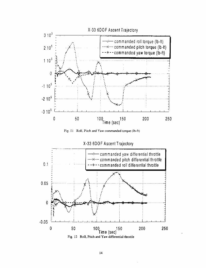
X-33 6DOF Ascent Trajectory3 105 , , ,

_- .., ,: commanded rolltorque (Ib-ft)4 ,

2 105 - ....... :"---"............. ----×----commanded pitch torque (Ib-ft)i ,' t

" .' ' --_--commanded yaw torque (Ib-ft),,-_ ,, ,

1 105 -t .' .6_..... ,,....... ",, "...............................,N, '_..................................I| i .s o f b

-1 105 " ' : " ' ' '_'"'................... %..... _;. ',.............',. ; : .,,, : ; :;

2 105 -_" ........... "-......... r. . ° t

I. I J.

. , """X-.-,',:

-3105 ' , i,,,, i,,,, i,,, J , , , ,

0 50 100 150 200 250Time (sec)

Fig. 11 Roll, Pitch and Yaw commanded torque (lb-ft)


- I _ commanded yaw differential throttle.... ×----commanded pitch differential throttle

0.1 ..... --_--commanded roll differential throttle

,..,_ "_.." :',,.

. •o o . o *

0.05 ................. : ....... "-_...... : ..... ,'-'.......... :---xz_-............................

,./I I

1 "" : ',- , t ,

.005 ! , : r =i,,. _, J I I J I i, u r , l I , I x

0 50 100._imle (sec)150 200 250Fig. ].2 Roll, Pitch and Yaw differential throttle

].4

X-33 6D©F Ascent Trajectoryf ] i i , , ,

sensed right flap deflection (degree)15 ...................×---- sensed left flap deflection (degree)

,.. - ,,". .... i .................................. ; ............... --_

1 _-...................... ,- : : : ,_ "a i . ..,

fl . . !

3

0

-5 ' - ......... s_. .................. t. ................. ,.................. ,. ................

i QI i ,

e

0 50 100 150 200 250Time (sec)

Fig. 13 Sensed flap deflections

10_X-33 6DOFAscent Trajectory

-5

e sensed right inboardelevon deflection(de_ree)....:.:----sensed left inboard elevon deflection(degree)

-IL i

50 100Time (sec)150 200 250

Fig. 14 Sensed inboard elevon deflections

15

10X-33 6DOF Ascent Trajectory

- " sensed right outboard eleven deflection (degree)

.... ×----sensed left outboard eleven deflection (degree)i

=5 t _ I L r , , t I _ ' [ 1 1 I 1 I ', L

0 50 100Time (sec)150 200 250

Fig. 15 Sensed outboard elevon deflections


4 L .... ] e sensed right rudier'de'flecti'on (degree) i- ,_ ] .... :-:----sensed left rudder deflection (degree)

3 _ , ................

It

0 50 100- imeT (sec) 150 200 250

Fig. 16 Sensed rudder deflections

16


0.05

-0.05

Fig. 17

-#

|Q..-ii

I'

i

-_ sensed rolltracking error(rad)

.... x---. sensed pitch tracking error (rad)

- -._- -sensed yaw tracking error (rad)

:. : !,MS _1.Ibll

/\,,. ',,../':; : ,,"-..__, t • | x .o , *

i .i

Ill1 IFll 11! Illl

0 50 100 150 200 250Time (sec)

Sensed orientation angle tracking errors given power pack out at 100 sec.

17

Sliding Mode Control of the X-33 With an Engine Failure ... · PDF fileSliding Mode Control of...

Documents

Transcript of Sliding Mode Control of the X-33 With an Engine Failure ... · PDF fileSliding Mode Control of...