APEURO Lecture 3B Mrs. Kray slides taken from Ms. Susan M. Pojer English Constitutional Monarchy.
Upload
arthur-charpentierCategory
view
6.441download
1
Arthur CHARPENTIER - Welfare, Inequality and Poverty
Arthur Charpentier
http ://freakonometrics.hypotheses.org/
Université de Rennes 1, January 2015
Welfare, Inequality & Poverty, # 3
1

Arthur CHARPENTIER - Welfare, Inequality and Poverty
Inequality Comparisons (2-person Economy)not much to say... any measure of dispersion is appropriate
– income gap x2 − x1
– proportional gap x2
x1– any functional of the distance√
|x2 − x1|
graphs are from Amiel & Cowell (1999,ebooks.cambridge.org )
2

Arthur CHARPENTIER - Welfare, Inequality and Poverty
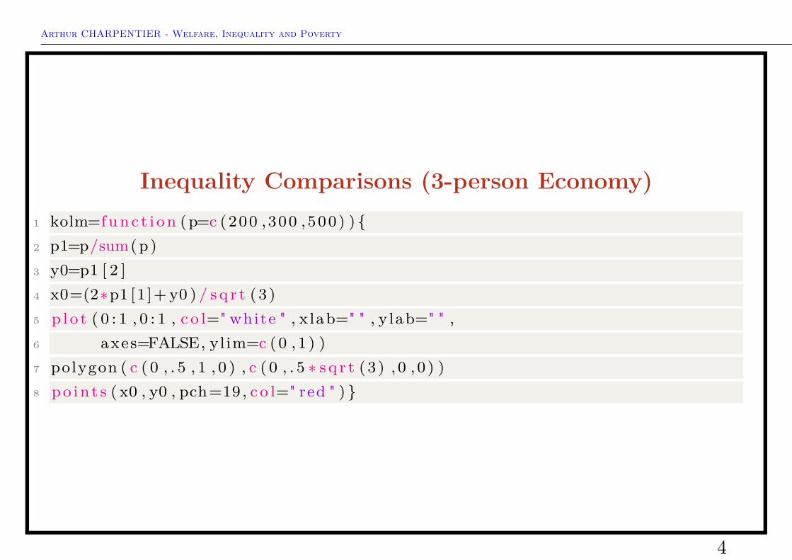
Inequality Comparisons (3-person Economy)Consider any 3-person economy, with incomes x = {x1, x2, x3}. This point can bevisualized in Kolm triangle.
3
Arthur CHARPENTIER - Welfare, Inequality and Poverty
Inequality Comparisons (3-person Economy)1 kolm=f u n c t i o n (p=c (200 ,300 ,500) ) {2 p1=p/sum(p)3 y0=p1 [ 2 ]4 x0=(2∗p1 [1 ]+ y0 ) / s q r t (3 )5 p l o t ( 0 : 1 , 0 : 1 , c o l=" white " , x lab=" " , ylab=" " ,6 axes=FALSE, ylim=c ( 0 , 1 ) )7 polygon ( c ( 0 , . 5 , 1 , 0 ) , c ( 0 , . 5 ∗ s q r t (3 ) , 0 , 0 ) )8 p o in t s ( x0 , y0 , pch=19, c o l=" red " ) }
4

Arthur CHARPENTIER - Welfare, Inequality and Poverty
Inequality Comparisons (n-person Economy)In a n-person economy, comparison are clearly more difficult
5

Arthur CHARPENTIER - Welfare, Inequality and Poverty
Inequality Comparisons (n-person Economy)Why not look at inequality per subgroups,
If we focus at the top of the distribution(same holds for the bottom),→ rising inequality
If we focus at the middle of the distri-bution,→ falling inequality
6

Arthur CHARPENTIER - Welfare, Inequality and Poverty
Inequality Comparisons (n-person Economy)To measure inequality, we usually– define ‘equality’ based on some reference point / distribution– define a distance to the reference point / distribution– aggregate individual distancesWe want to visualize the distribution of incomes
1 > income <− read . csv ( " http : //www. v c h a r i t e . univ−mrs . f r /pp/ lubrano /cours / f e s 9 6 . csv " , sep=" ; " , header=FALSE) $V1
F (x) = P(X ≤ x) =∫ x
0f(t)dt
7
Arthur CHARPENTIER - Welfare, Inequality and Poverty
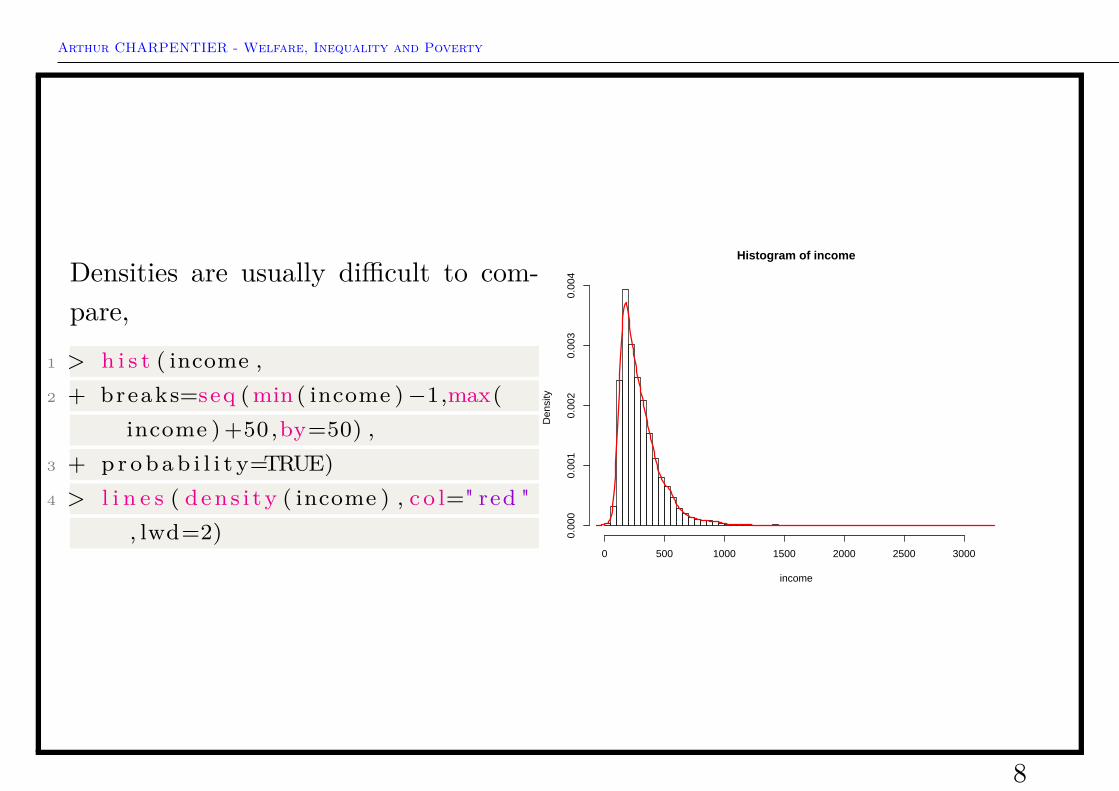
Densities are usually difficult to com-pare,
1 > h i s t ( income ,2 + breaks=seq ( min ( income ) −1,max(
income ) +50,by=50) ,3 + p r o b a b i l i t y=TRUE)4 > l i n e s ( d e ns i ty ( income ) , c o l=" red "
, lwd=2)
Histogram of income
income
Den
sity
0 500 1000 1500 2000 2500 3000
0.00
00.
001
0.00
20.
003
0.00
4
8
Arthur CHARPENTIER - Welfare, Inequality and Poverty
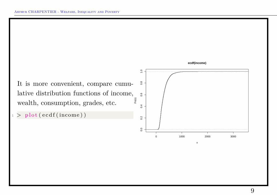
It is more convenient, compare cumu-lative distribution functions of income,wealth, consumption, grades, etc.
1 > p l o t ( ecd f ( income ) )
0 1000 2000 3000
0.0
0.2
0.4
0.6
0.8
1.0
ecdf(income)
x
Fn(
x)
9
Arthur CHARPENTIER - Welfare, Inequality and Poverty
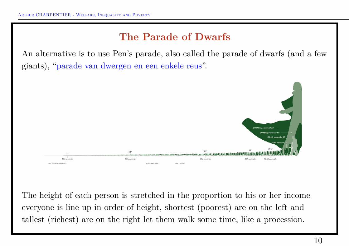
The Parade of DwarfsAn alternative is to use Pen’s parade, also called the parade of dwarfs (and a fewgiants), “parade van dwergen en een enkele reus”.
The height of each person is stretched in the proportion to his or her incomeeveryone is line up in order of height, shortest (poorest) are on the left andtallest (richest) are on the right let them walk some time, like a procession.
10

Arthur CHARPENTIER - Welfare, Inequality and Poverty
c.d.f., quantiles and Lorenz
1 > Pen ( income )
0.0 0.2 0.4 0.6 0.8 1.0
0
2
4
6
8
10
Pen's Parade
i n
x (i)
x
11

Arthur CHARPENTIER - Welfare, Inequality and Poverty
c.d.f., quantiles and LorenzThis parade of the Dwarfs function is just the quantile function.
1 > q <− f u n c t i o n (u) q u a n t i l e (income , u)
see also1 > n <− l ength ( income )2 > u <− seq (1 / (2 ∗n) ,1−1/ (2 ∗n) ,
l ength=n)3 > p l o t (u , s o r t ( income ) , type=" l " )
p l o t ( ecd f ( income ) ) 0.0 0.2 0.4 0.6 0.8 1.0
050
010
0015
0020
0025
0030
00
u
sort
(inco
me)
12

Arthur CHARPENTIER - Welfare, Inequality and Poverty
c.d.f., quantiles and LorenzTo get Lorentz curve, we substitute on the y-axis proportion of incomes toincomes.
1 > l i b r a r y ( ineq )2 > Lc ( income )3 > L <− f u n c t i o n (u) Lc ( income ) $L [
round (u∗ l ength ( income ) ) ]
0.0 0.2 0.4 0.6 0.8 1.0
0.0
0.2
0.4
0.6
0.8
1.0
Lorenz curve
p
L(p)
13

Arthur CHARPENTIER - Welfare, Inequality and Poverty
c.d.f., quantiles and Lorenz
x-axis y-axis
c.d.f. income proportion of populationPen’s parade(quantile)
proportion of population income
Lorenz curve proportion of population proportion of income
14

Arthur CHARPENTIER - Welfare, Inequality and Poverty
Standard statistical measure of dispersionThe variance for a sample X = {x1, · · · , xn} is
Var(X) = 1n
n∑i=1
[xi − x]2
where the baseline (reference) is x = 1n
n∑i=1
xi.
1 > var ( income )2 [ 1 ] 34178.43
problem it is a quadratic function, Var(αX) = α2Var(X).
15
Arthur CHARPENTIER - Welfare, Inequality and Poverty
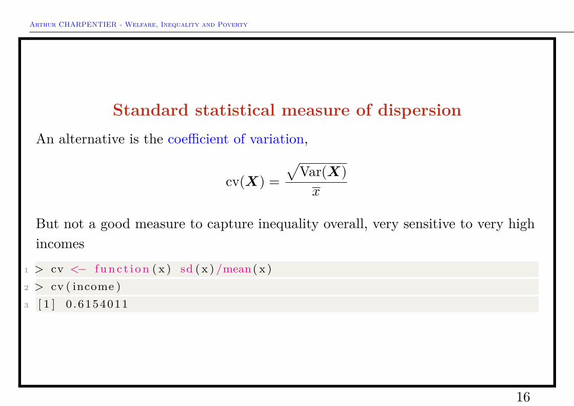
Standard statistical measure of dispersionAn alternative is the coefficient of variation,
cv(X) =√
Var(X)x
But not a good measure to capture inequality overall, very sensitive to very highincomes
1 > cv <− f u n c t i o n ( x ) sd ( x ) /mean( x )2 > cv ( income )3 [ 1 ] 0 .6154011
16

Arthur CHARPENTIER - Welfare, Inequality and Poverty
Standard statistical measure of dispersionAn alternative is to use a logarithmic transformation. Use the logarithmicvariance
Varlog(X) = 1n
n∑i=1
[log(xi)− log(x)]2
1 > var_log <− f u n c t i o n ( x ) var ( l og ( x ) )2 > var_log ( income )3 [ 1 ] 0 .2921022
Those measures are distances on the x-axis.
17

Arthur CHARPENTIER - Welfare, Inequality and Poverty
Standard statistical measure of dispersionOther inequality measures can be derived from Pen’s parade of the Dwarfs, wheremeasures are based on distances on the y-axis, i.e. distances between quantiles.
Qp = F−1(p) i.e. F (Qp) = p
e.g. the median is the quantile when p = 50%, the first quartile is the quantilewhen p = 25%, the first quintile is the quantile when p = 20%, the first decile isthe quantile when p = 10%, the first percentile is the quantile when p = 1%
1 > q u a n t i l e ( income , c ( . 1 , . 5 , . 9 , . 9 9 ) )2 10% 50% 90% 99%3 137.6294 253.9090 519.6887 933.9211
18

Arthur CHARPENTIER - Welfare, Inequality and Poverty
Standard statistical measure of dispersionDefine the quantile ratio as
Rp = Q1−p
Qp
In case of perfect equality, Rp = 1.
The most popular one is probably the90/10 ratio.
1 > R_p <− f u n c t i o n (x , p) q u a n t i l e (x,1−p) / q u a n t i l e (x , p )
2 > R_p( income , . 1 )3 90%4 3 .776
0.0 0.2 0.4 0.6 0.8 1.0
05
1015
probability
R
This index measures the gap between the rich and the poor.
19

Arthur CHARPENTIER - Welfare, Inequality and Poverty
E.g. R0.1 = 10 means that top 10% incomes are more than 10 times higher thanthe bottom 10% incomes.
Ignores the distribution (apart from the two points), violates transfer principle.
An alternative measure might be Kuznets Ratio, defined from Lorenz curve asthe ratio of the share of income earned by the poorest p share of the populationand the richest r share of the population,
I(p, r) = L(p)1− L(1− r)
But here again, it ignores the distribution between the cutoffs and thereforeviolates the transfer principle.
20

Arthur CHARPENTIER - Welfare, Inequality and Poverty
An alternative measure can be the IQR,interquantile ratio,
IQRp = Q1−p −QpQ0.5
1 > IQR_p <− f u n c t i o n (x , p) (q u a n t i l e (x,1−p)−q u a n t i l e (x , p)) / q u a n t i l e (x , . 5 )
2 > IQR_p( income , . 1 )3 90%4 1.504709
0.0 0.1 0.2 0.3 0.4 0.5
01
23
4
probabilityIQ
R
Problem only focuses on top (1− p)-th and bottom p-th proportion. Does notcare about what happens between those quantiles.
21

Arthur CHARPENTIER - Welfare, Inequality and Poverty
Standard statistical measure of dispersionPen’s parade suggest to measure thegreen area, for some p ∈ (0, 1), Mp,
1 > M_p <− f u n c t i o n (x , p) {2 a <− seq (0 , p , l ength =251)3 b <− seq (p , 1 , l ength =251)4 ya <− q u a n t i l e (x , p )−q u a n t i l e (x ,
a )5 a1 <− sum ( ( ya [ 1 : 2 50 ] + ya [ 2 : 2 5 1 ] )
/2∗p/ 250)6 yb <− q u a n t i l e (x , b )−q u a n t i l e (x ,
p )7 a2 <− sum ( ( yb [ 1 : 2 50 ] + yb [ 2 : 2 5 1 ] )
/2∗(1−p) / 250)8 r e turn ( a1+a2 ) }
22
Arthur CHARPENTIER - Welfare, Inequality and Poverty
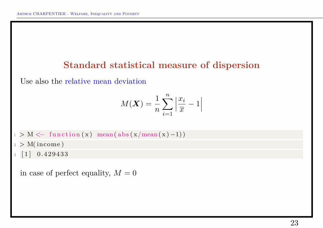
Standard statistical measure of dispersionUse also the relative mean deviation
M(X) = 1n
n∑i=1
∣∣∣xix− 1∣∣∣
1 > M <− f u n c t i o n ( x ) mean( abs ( x/mean( x ) −1) )2 > M( income )3 [ 1 ] 0 .429433
in case of perfect equality, M = 0
23
Arthur CHARPENTIER - Welfare, Inequality and Poverty
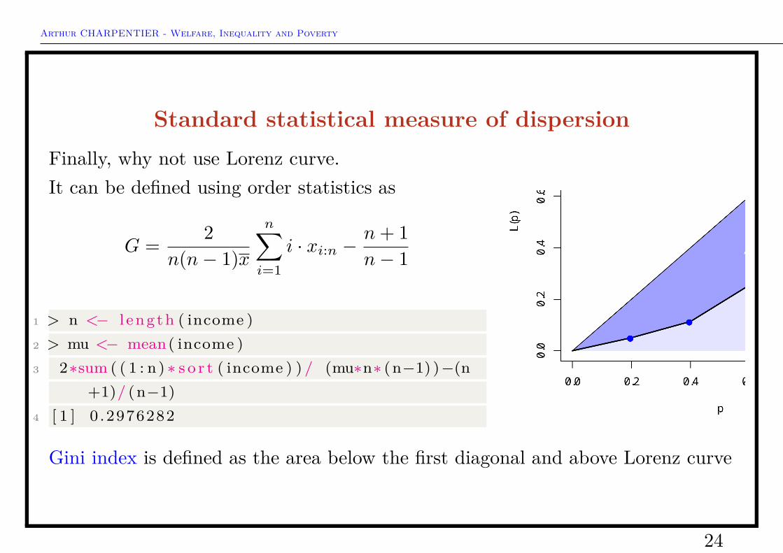
Standard statistical measure of dispersionFinally, why not use Lorenz curve.It can be defined using order statistics as
G = 2n(n− 1)x
n∑i=1
i · xi:n −n+ 1n− 1
1 > n <− l ength ( income )2 > mu <− mean( income )3 2∗sum ( ( 1 : n) ∗ s o r t ( income ) ) / (mu∗n∗ (n−1) )−(n
+1)/ (n−1)4 [ 1 ] 0 .2976282
Gini index is defined as the area below the first diagonal and above Lorenz curve
24

Arthur CHARPENTIER - Welfare, Inequality and Poverty
Standard statistical measure of dispersion
G(X) = 12n2x
n∑i,j=1
|xi − xj |
Perfect equality is obtained when G = 0.
Remark Gini index can be related to the variance or the coefficient of variation,since
Var(X) = 1n
n∑i=1
[xi − x]2 = 1n2
n∑i,j=1
(xi − xj)2
Here,
G(X) = ∆(X)2x with ∆(X) = 1
n2
n∑i,j=1
|xi − xj |
1 > ineq ( income , " Gini " )2 [ 1 ] 0 .2975789
25

Arthur CHARPENTIER - Welfare, Inequality and Poverty
Axiomatic Approach for Inequality IndicesNeed some rules to say if a principle used to divide a cake of fixed size amongst afixed number of people is fair, on not.
A standard one is the Anonymity Principle. Let X = {x1, · · · , xn}, then
I(x1, x2, · · · , xn) = I(x2, x1, · · · , xn)
also called Replication Invariance Principle
The Transfert Principle
for any given income distribution if you take a small amount of income from oneperson and give it to a richer person then income inequality must increase
Pigou (1912) and Dalton (1920), a transfer from a richer to a poorer person willdecrease inequality. Let X = {x1, · · · , xn} with x1 ≤ · · · ≤ xn, then
I(x1, · · · , xi, · · · , xj , · · · , xn) > I(x1, · · · , xi+δ, · · · , xj−δ, · · · , xn)
26
Arthur CHARPENTIER - Welfare, Inequality and Poverty
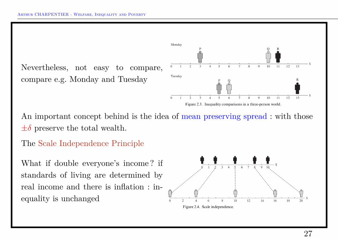
Nevertheless, not easy to compare,compare e.g. Monday and Tuesday
An important concept behind is the idea of mean preserving spread : with those±δ preserve the total wealth.
The Scale Independence Principle
What if double everyone’s income ? ifstandards of living are determined byreal income and there is inflation : in-equality is unchanged
27

Arthur CHARPENTIER - Welfare, Inequality and Poverty
Let X = {x1, · · · , xn}, then
I(λx1, · · · , λxn) = I(x1, · · · , xn)
also called Zero-Degree Homogeneity property.
The Population Principle
Consider clones of the economy
I(x1, · · · , x1︸ ︷︷ ︸k times
, · · · , xn, · · · , xn︸ ︷︷ ︸k times
) = I(x1, · · · , xn)
28

Arthur CHARPENTIER - Welfare, Inequality and Poverty
Is it really that simple ?
The Decomposability Principle
Assume that we can decompose inequality by subgroups (based on gender, race,coutries, etc)
According to this principle, if inequality increases in a subgroup, it increases inthe whole population, ceteris paribus
I(x1, · · · , xn, y1, · · · , yn) ≤ I(x?1, · · · , x?n, y1, · · · , yn)
as long as I(x1, · · · , xn) ≤ I(x?1, · · · , x?n).
29

Arthur CHARPENTIER - Welfare, Inequality and Poverty
Consider two groups, X and X?
Then add the same subgroup Y to bothX and X?
30

Arthur CHARPENTIER - Welfare, Inequality and Poverty
Axiomatic Approach for Inequality IndicesAny inequality measure that simultaneously satisfies the properties of theprinciple of transfers, scale independence, population principle anddecomposability must be expressible in the form
Eξ = 1ξ2 − ξ
(1n
n∑i=1
(xix
)ξ− 1)
for some ξ ∈ R. This is the generalized entropy measure.1 > entropy ( income , 0 )2 [ 1 ] 0 .14566043 > entropy ( income , . 5 )4 [ 1 ] 0 .14461055 > entropy ( income , 1 )6 [ 1 ] 0 .15069737 > entropy ( income , 2 )8 [ 1 ] 0 .1893279
31

Arthur CHARPENTIER - Welfare, Inequality and Poverty
The higher ξ, the more sensitive to high incomes.
Remark rule of thumb, take ξ ∈ [−1,+2].
When ξ = 0, the mean logarithmic deviation (MLD),
MLD = E0 = − 1n
n∑i=1
log(xix
)When ξ = 1, the Theil index
T = E1 = 1n
n∑i=1
xix
log(xix
)1 > Thei l ( income )2 [ 1 ] 0 .1506973
When ξ = 2, the index can be related to the coefficient of variation
E2 = [coefficient of variation]2
2
32
Arthur CHARPENTIER - Welfare, Inequality and Poverty
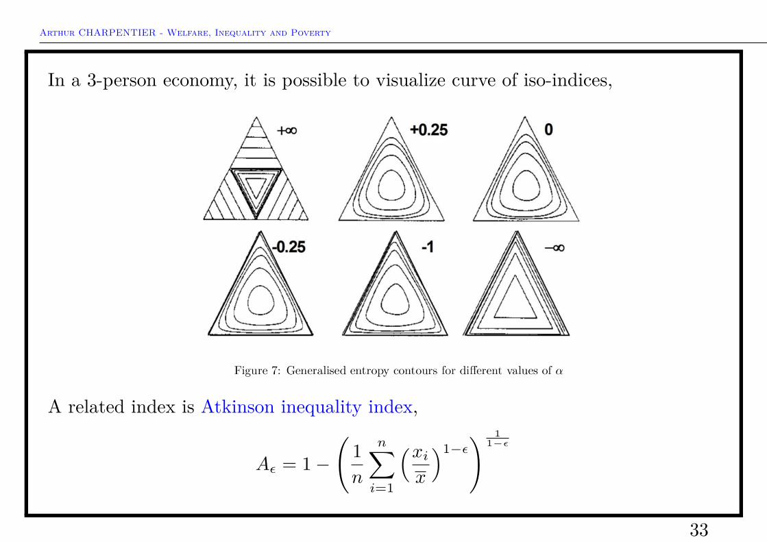
In a 3-person economy, it is possible to visualize curve of iso-indices,
A related index is Atkinson inequality index,
Aε = 1−(
1n
n∑i=1
(xix
)1−ε) 1
1−ε
33

Arthur CHARPENTIER - Welfare, Inequality and Poverty
with ε ≥ 0.1 > Atkinson ( income , 0 . 5 )2 [ 1 ] 0 .070998243 > Atkinson ( income , 1 )4 [ 1 ] 0 .1355487
In the case where ε→ 1, we obtain
A1 = 1−n∏i=1
(xix
() 1n
ε is usually interpreted as an aversion to inequality index.
Observe thatAε = 1− [(ε2 − ε)E1−ε + 1]
11−ε
and the limiting case A1 = 1− exp[−E0].
Thus, the Atkinson index is ordinally equivalent to the GE index, since theyproduce the same ranking of different distributions.
34

Arthur CHARPENTIER - Welfare, Inequality and Poverty
Consider indices obtained when X isobtained from a LN(0, σ2) distributionand from a P(α) distribution.
35

Arthur CHARPENTIER - Welfare, Inequality and Poverty
Changing the AxiomsIs there an agreement about the axioms ?
For instance, no unanimous agreement on the scale independence axiom,
Why not a translation independence axiom ?
Translation Independence Principle : if every incomes are increased by the sameamount, the inequality measure is unchanged
Given X = (x1, · · · , xn),
I(x1, · · · , xn) = I(x1 + h, · · · , xn + h)
If we change the scale independence principle by this translation independence,we get other indices.
36

Arthur CHARPENTIER - Welfare, Inequality and Poverty
Changing the AxiomsKolm indices satisfy the principle of transfers, translation independence,population principle and decomposability
Kθ = log(
1n
n∑i=1
eθ[xi−x]
)
1 > Kolm( income , 1 )2 [ 1 ] 291.58783 > Kolm( income , . 5 )4 [ 1 ] 283.9989
37

Arthur CHARPENTIER - Welfare, Inequality and Poverty
From Measuring to OrderingOver time, between countries, before/after tax, etc.
X is said to be Lorenz-dominated by Y if LX ≤ LY . In that case Y is moreequal, or less inequal.
In such a case, X can be reached from Y by a sequence of poorer-to-richerpairwiser income transfers.
In that case, any inequality measure satisfying the population principle, scaleindependence, anonymity and principle of transfers axioms are consistent withthe Lorenz dominance (namely Theil, Gini, MLD, Generalized Entropy andAtkinson).
Remark A regressive transfer will move the Lorenz curve further away from thediagonal. So satisfies transfer principle. And it satisfies also the scale invarianceproperty.
38

Arthur CHARPENTIER - Welfare, Inequality and Poverty
Example if Xi ∼ P(αi, xi),
LX1 ≤ LX2 ←→ α1 ≤ α2
and if Xi ∼ LN(µi, σ2i ),
LX1 ≤ LX2 ←→ σ21 ≥ σ2
2
Lorenz dominance is a relation that is incomplete : when Lorenz curves cross, thecriterion cannot decide between the two distributions.
→ the ranking is considered unambiguous.
Further, one should take into account possible random noise.
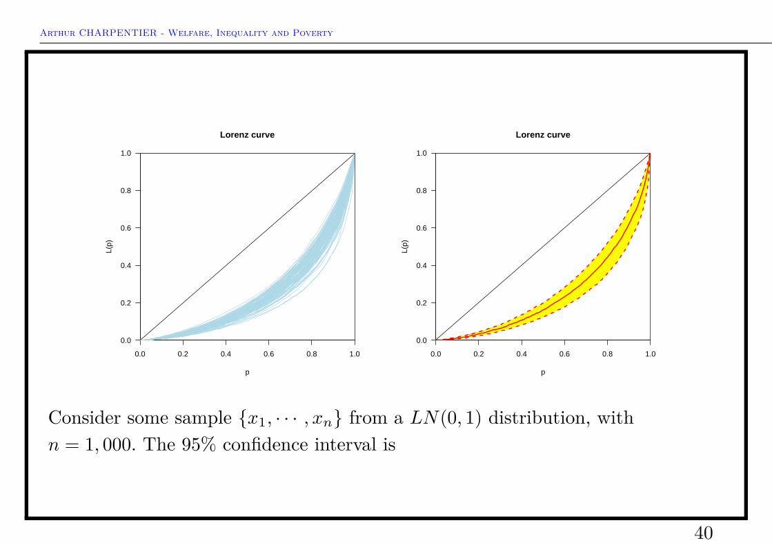
Consider some sample {x1, · · · , xn} from a LN(0, 1) distribution, with n = 100.The 95% confidence interval is
39
Arthur CHARPENTIER - Welfare, Inequality and Poverty
0.0 0.2 0.4 0.6 0.8 1.0
0.0
0.2
0.4
0.6
0.8
1.0
Lorenz curve
p
L(p)
0.0 0.2 0.4 0.6 0.8 1.0
0.0
0.2
0.4
0.6
0.8
1.0
Lorenz curve
p
L(p)
Consider some sample {x1, · · · , xn} from a LN(0, 1) distribution, withn = 1, 000. The 95% confidence interval is
40

Arthur CHARPENTIER - Welfare, Inequality and Poverty
0.0 0.2 0.4 0.6 0.8 1.0
0.0
0.2
0.4
0.6
0.8
1.0
Lorenz curve
p
L(p)
0.0 0.2 0.4 0.6 0.8 1.0
0.0
0.2
0.4
0.6
0.8
1.0
Lorenz curve
pL(
p)
41
Arthur CHARPENTIER - Welfare, Inequality and Poverty
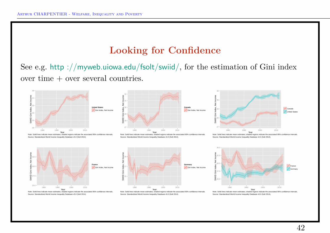
Looking for ConfidenceSee e.g. http ://myweb.uiowa.edu/fsolt/swiid/, for the estimation of Gini indexover time + over several countries.
29
31
33
35
37
39
1980 1990 2000 2010Year
SW
IID G
ini I
ndex
, Net
Inco
me
United States
Gini Index, Net Income
Note: Solid lines indicate mean estimates; shaded regions indicate the associated 95% confidence intervals.Source: Standardized World Income Inequality Database v5.0 (Solt 2014).
27
28
29
30
31
32
1980 1990 2000 2010Year
SW
IID G
ini I
ndex
, Net
Inco
me
Canada
Gini Index, Net Income
Note: Solid lines indicate mean estimates; shaded regions indicate the associated 95% confidence intervals.Source: Standardized World Income Inequality Database v5.0 (Solt 2014).
27
30
33
36
39
1980 1990 2000 2010Year
SW
IID G
ini I
ndex
, Net
Inco
me
Canada
United States
Note: Solid lines indicate mean estimates; shaded regions indicate the associated 95% confidence intervals.Source: Standardized World Income Inequality Database v5.0 (Solt 2014).
25.0
27.5
30.0
32.5
1980 1990 2000 2010Year
SW
IID G
ini I
ndex
, Net
Inco
me
France
Gini Index, Net Income
Note: Solid lines indicate mean estimates; shaded regions indicate the associated 95% confidence intervals.Source: Standardized World Income Inequality Database v5.0 (Solt 2014).
25
27
29
1980 1990 2000 2010Year
SW
IID G
ini I
ndex
, Net
Inco
me
Germany
Gini Index, Net Income
Note: Solid lines indicate mean estimates; shaded regions indicate the associated 95% confidence intervals.Source: Standardized World Income Inequality Database v5.0 (Solt 2014).
25.0
27.5
30.0
32.5
35.0
1980 1990 2000 2010Year
SW
IID G
ini I
ndex
, Net
Inco
me
France
Germany
Note: Solid lines indicate mean estimates; shaded regions indicate the associated 95% confidence intervals.Source: Standardized World Income Inequality Database v5.0 (Solt 2014).
42
Arthur CHARPENTIER - Welfare, Inequality and Poverty
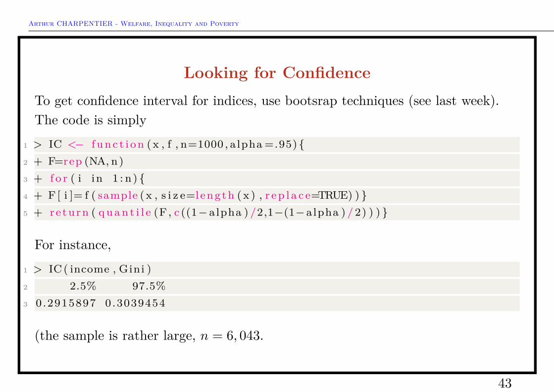
Looking for ConfidenceTo get confidence interval for indices, use bootsrap techniques (see last week).The code is simply
1 > IC <− f u n c t i o n (x , f , n=1000 , alpha =.95) {2 + F=rep (NA, n)3 + f o r ( i in 1 : n ) {4 + F [ i ]= f ( sample (x , s i z e=length ( x ) , r e p l a c e=TRUE) ) }5 + return ( q u a n t i l e (F , c ((1− alpha ) /2,1−(1− alpha ) / 2) ) ) }
For instance,1 > IC ( income , Gini )2 2.5% 97.5%3 0.2915897 0.3039454
(the sample is rather large, n = 6, 043.
43

Arthur CHARPENTIER - Welfare, Inequality and Poverty
Looking for Confidence1 > IC ( income , Gini )2 2.5% 97.5%3 0.2915897 0.30394544 > IC ( income , The i l )5 2.5% 97.5%6 0.1421775 0.15950127 > IC ( income , entropy )8 2.5% 97.5%9 0.1377267 0.1517201
44
Arthur CHARPENTIER - Welfare, Inequality and Poverty
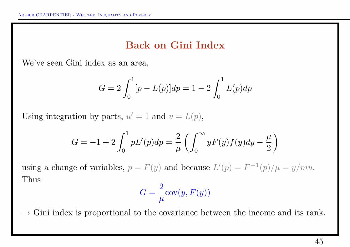
Back on Gini IndexWe’ve seen Gini index as an area,
G = 2∫ 1
0[p− L(p)]dp = 1− 2
∫ 1
0L(p)dp
Using integration by parts, u′ = 1 and v = L(p),
G = −1 + 2∫ 1
0pL′(p)dp = 2
µ
(∫ ∞0
yF (y)f(y)dy − µ
2
)using a change of variables, p = F (y) and because L′(p) = F−1(p)/µ = y/mu.Thus
G = 2µcov(y, F (y))
→ Gini index is proportional to the covariance between the income and its rank.
45
Arthur CHARPENTIER - Welfare, Inequality and Poverty
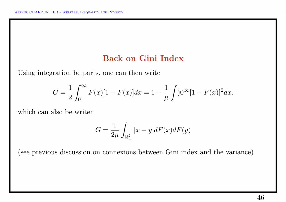
Back on Gini IndexUsing integration be parts, one can then write
G = 12
∫ ∞0
F (x)[1− F (x)]dx = 1− 1µ
∫)0∞[1− F (x)]2dx.
which can also be writen
G = 12µ
∫R2
+
|x− y|dF (x)dF (y)
(see previous discussion on connexions between Gini index and the variance)
46

Arthur CHARPENTIER - Welfare, Inequality and Poverty
Decomposition(s)When studying inequalities, it might be interesting to discussion possibledecompostions either by subgroups, or by sources,
– subgroups decomposition, e.g Male/Female, Rural/Urban see FAO (2006,fao.org)
– source decomposition, e.g earnings/gvnt benefits/investment/pension, etc, seeslide 41 #1 and FAO (2006, fao.org)
For the variance, decomposition per groups is related to ANOVA,
Var(Y ) = E[Var(Y |X)]︸ ︷︷ ︸within
+Var(E[Y |X])︸ ︷︷ ︸between
Hence, if X ∈ {x1, · · · , xk} (k subgroups),
Var(Y ) =∑k
pkVar(Y | group k)︸ ︷︷ ︸within
+Var(E[Y |X])︸ ︷︷ ︸between
47
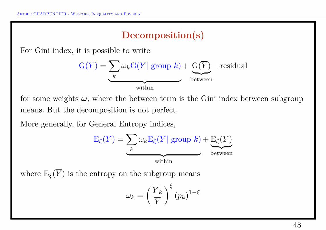
Arthur CHARPENTIER - Welfare, Inequality and Poverty
Decomposition(s)For Gini index, it is possible to write
G(Y ) =∑k
ωkG(Y | group k)︸ ︷︷ ︸within
+ G(Y )︸ ︷︷ ︸between
+residual
for some weights ω, where the between term is the Gini index between subgroupmeans. But the decomposition is not perfect.
More generally, for General Entropy indices,
Eξ(Y ) =∑k
ωkEξ(Y | group k)︸ ︷︷ ︸within
+ Eξ(Y )︸ ︷︷ ︸between
where Eξ(Y ) is the entropy on the subgroup means
ωk =(Y k
Y
)ξ(pk)1−ξ
48

Arthur CHARPENTIER - Welfare, Inequality and Poverty
Decomposition(s)Now, a decomposition per source, i.e. Yi = Y1,i + · · ·+ Yk,i + · · · , among sources.
For Gini index natural decomposition was suggested by Lerman & Yitzhaki(1985, jstor.org)
G(Y ) = 2Ycov(Y, F (Y )) =
∑k
2Ycov(Yk, F (Y ))︸ ︷︷ ︸k-th contribution
thus, it is based on the covariance between the k-th source and the ranks basedon cumulated incomes.
Similarly for Theil index,
T (Y ) =∑k
1n
∑i
(Yk,i
Y
)log(Yi
Y
)︸ ︷︷ ︸
k-th contribution
49

Arthur CHARPENTIER - Welfare, Inequality and Poverty
Decomposition(s)It is possible to use Shapley value for decomposition of indices I(·). Consider mgroups, N = {1, · · · ,m}, and definie I(S) = I(xS) where S ⊂ N . Then Shapleyvalue yields
φk(v) =∑
S⊆N\{k}
|S|! (m− |S| − 1)!m! (I(S ∪ {k})− I(S))
50