
Stack of coins calculator economic growth powerpoint presentation slides.
Upload
muthannCategory
view
487download
0
Growth Theory
PD Dr. M. Pasche
DFG Research Training Group “The Economics of Innovative Change”,
Friedrich Schiller University Jena
Creative Commons by 3.0 license – 2008/2013 (except for included graphics from other sources)
Work in progress. Bug Report to: [email protected]
S.1

Outline:
1. The Empirical Picture of Growth
1.1 Some Stylized Facts1.2 Convergence1.3 Growth Accounting1.4 Regressions on Growth Determinants
2. Some Preliminaries of Growth Theory
2.1 The Harrod-Domar Approach2.2 The Basic Solow Model2.3 Exogenous Technological Change2.4 Intertemporal Optimization2.5 Analyzing Growth Equilibria
3. Models of Endogenous Growth
3.1 Overview: Sources of Growth3.2 AK model and Knowledge Spillovers3.3 Models with Human Capital Accumulation3.4 R&D based Growth with Increasing Product Variety3.5 R&D based Growth with Increasing Product Quality3.6 Technological Progress, Diffusion, and Human Capital3.7 Further Issues
S.2

4. Critique and an Evolutionary Perspective
4.1 Empirical Evidence4.2 Methodological Objections4.3 Evolutionary Approaches: Outline4.4 Evolutionary Approaches: Example
Basic Literature:
* Barro, R.J., Sala-i-Martin, X. (1995), Economic Growth. New York:McGraw-Hill.
* Aghion, P., Howitt, P. (2009), The Economics of Growth. MITPress.
Acemoglu, D. (2008), Introduction to Modern Economic Growth.Princeton University Press.
References to more specific literature can be found in the slide collection.
S.3

1. The Empirical Picture of Growth1.1 Some Stylized Facts
Literature:
Barro, R.E., Sala-i-Martin, X. (1995), Economic Growth.Chapter 1.1-1.2 (chapter 10-12 for a deep empirical analysis)
Kaldor, N. (1963), Capital Accumulation and Economic Growth, in:Lutz, F.A., Hague, D.C. (eds.), Proceedings of a Conference held bythe International Economics Association. London: Macmillan.
Mankiw, N.G., Romer, D., Weil, D.N. (1992), A Contribution to theEmpirics of Economic Growth. Quarterly Journal of Economics107(2), 407-437
Temple, J. (1999), The New Growth Evidence. Journal of EconomicLiterature 37(1), 112-156.
Symbols:
Y = A · F (K ,N) = real output or incomeK = capital stockN = employed laborA = total factor productivityr = real interest ratew = real wages
S.4

1. The Empirical Picture of Growth1.1 Some Stylized Facts
Income per capita y = Y /N is growing with a constant rate (butdeclining growth rate in the 1970ies in most developped countries).
The capital/output ratio (capital coefficient) K/Y is stationary.
The capital/labor ratio (capital intensity) K/N is increasing. This isjust an implication of a growing Y /N and a stationary K/Y .
The rate of return to capital r = ∂Y /∂K is stationary (but has acertain decline in developped countries).
The income distribution is stationary (measured by V = rk/wN orby wN/Y , rK/Y ).
The rate of return to labor w = ∂Y /∂N is increasing. This is justan implication of stationary distribution, stationary K/Y andgrowing Y /N.
The per capita growth rates differ much across countries.
The per capita growth rate cannot be explained solely byaccumulation of capital and growing labor force (→ technicalprogress, human capital, knowledge etc.).
S.5

1. The Empirical Picture of Growth1.1 Some Stylized Facts
A note on growth rates:
Growth with a constant rate g means that the variable growsexponentially:
y(t) = y(0)egt
Logarithm and differentiating with respect to time:
ln y(t) = ln y(0) + gt ⇒ gy ≡d ln y(t)
dt=
1
y·dy
dt= g
For empirical data we use the first differences ∆ ln y(t) todetermine the growth rate.
Growth with a constant rate means that we have a linear trend ofln y(t) in a figure with absolute scale, or, alternatively, a lineartrend of y(t) in a figure with a logarithmic scale.
S.6

1. The Empirical Picture of Growth1.1 Some Stylized Facts
Some illustrating empirical facts on growth dynamics:
From 500 (roman imperium) to 1500: no significant economicgrowth!
1500-1800 about 0.1% growth rate. Moderate growth rates during the industrial revolution
1800-1900, increasing in the late 19th century. Massive acceleration of economic activity in the 20th century,
especially in the post war period. Decline of growth rates (in developped countries) starting
from the 1970ies.
Some illustrating empiricial facts on distribution (base = 2002):
The richest country is Luxembourg with $ 49368 per capita,the poorest country is Kongo with $ 344 (= factor 143!)
If Bangladesh grows with its average post war growth rate of1.1% then it approaches the 2002 level of per capita incomeof the USA in 200 years. S.7

1. The Empirical Picture of Growth1.1 Some Stylized Facts
S.8

1. The Empirical Picture of Growth1.1 Some Stylized Facts
S.9

1. The Empirical Picture of Growth1.2 Convergence
Are less developped countries growing faster(“catching-up”)?
Measuring convergence:
β-convergence: Negative relationship between per capitaincome y = Y /N and growth rate gy .
σ-convergence: Decline of a dispersion measure (likestandard deviation of (logarithmic) per capita income, Ginicoefficient etc.)
S.10

1. The Empirical Picture of Growth1.2 Convergence
Problems:
To be comparable, per capita income has to measured withthe same unit (e.g. Dollar). Hence we have to multiply thevalues with the exchange rate.
The exchange rates are fluctuating and are determined byvariables which are not related to real income (i.e.non-fundamental expectations). Thus, the per capita incomemeasured in a foreign currency may change even if ther realoutput remains the same: distortion of the measure.
Moreover, we have eventually different inflation rates in thecountries. Since we can measure the nominal income and theinflation rate, we have to account for the different purchasingpower when expressing the income in a foreign currency.
Solution: Construcing “purchasing power parity” exchange rates(PPP) to express all values in Dollar (e.g. Penn World tables)
S.11

1. The Empirical Picture of Growth1.2 Convergence
General result: There is no overall β-convergence!(Penn World Tables, x-axis = y1960, y-axis = gy as φ 1960-1992)
S.12

1. The Empirical Picture of Growth1.2 Convergence
Average growth rate of per capita income in 1960-1985 vs. ln(y) in 1960; 117
countries.
S.13

1. The Empirical Picture of Growth1.2 Convergence
Specific results: There is β-convergence within a group ofcountries which are “similar” regarding properties like high humancapital endowment, stable political institutions etc.
⇒ conditional β-convergence
⇒ “convergence clubs”
⇒ the gap between “rich” and “poor” countries is growing.
S.14

1. The Empirical Picture of Growth1.2 Convergence
Frequency of per capita income classes; 117 countries.
In 1960: E [ln(y)] = 7.296,V [ln(y)] = 0.81275,V /E = 0.1114.
S.15

1. The Empirical Picture of Growth1.2 Convergence
Frequency of per capita income classes; 117 countries.
In 1985: E [ln(y)] = 7.7959,V [ln(y)] = 1.2126,V /E = 0.1555.
S.16

1. The Empirical Picture of Growth1.3 Growth Accounting
Literature:
Solow, R.M. (1957), Technical Change and the AggregateProduction Function. Review of Economics and Statistics 39,312-320.
We start from a stylized production function Y = A · F (K ,N), whereA = A(t) is a time-dependend function for the total factor productivity(e.g. A = exp(ηt)).
Y (t) = A(t) · F (K (t),N(t))
lnY (t) = lnA(t) + lnF (K (t),N(t))
Differentiating with respect to time:
gY = gA +FK K
F+
FNN
F
= gA +AFK
YK +
AFN
YN
S.17

1. The Empirical Picture of Growth1.3 Growth Accounting
gY = gA +AFK
YK +
AFN
YN
with AFK = r and AFN = w we have
= gA +rK
Y
K
K+
wN
Y
N
N
and with a linear homogenous production function
= gA + α(t)gK + (1− α(t))gN
This can be transformed into an estimation equation for (non-observable)gA in discrete time.
Measuring Y ,K ,N the growth contributions of the physical inputs K andN can be estimated. The part of output growth which cannot beexplained by K and N is the “residual” which is interpreted as technicalprogress = increase in the total factor productivity (Solow residual).
S.18

1. The Empirical Picture of Growth1.3 Growth Accounting
Measuring Y : usually real GDP (from national statisticsagency)
Measuring N: number of employed and self-employed people,or: time measure (work hours)
Measuring K : This is non-trivial since the accounting systemsmeasure gross investment and depreciation.
Depreciation depends on legal regulation and is only a roughproxy for physical depreciation.
In balance sheets the “capital” is evaluated according todifferent and changing legislation rules.
Perpetual Inventory Method:
Kt = Kt−1 + I grosst − δKt−1
with δ ∈ (0, 1) as the constant depreciation rate.
S.19

1. The Empirical Picture of Growth1.3 Growth Accounting
Results:
S.20

1. The Empirical Picture of Growth1.3 Growth Accounting
Some problems:
Measuring the capital stock (see above), in addition we needestimates about the utilization of the present capital stock.Generally, the estimation results are often not robust for changes inthe measurement concept.
All qualitative changes in capital as well as in labor are capturedindirectly in the TFP. However, much progress is embodied in thephysical inputs. It is reasonable to disaggregate the inputs toaccount for these effects, e.g. including human capital ordistinguishing groups of different skilled worker (with differentaverage wages), or distinguishing capital vintages.
The empirical validity of constant returns of scale and competitivefactor markets is questionable.
Growth is also affected by non-technical determinants like stabilityof political institutions, tax system, integration into global markets,protection of intellectual property rights etc. Hence, institutionalchange is captured as “technological” change.
S.21

1. The Empirical Picture of Growth1.4 Regressions on Growth Determinants
Literature:
Mankiw, N.G., Romer, D., Weil, D.N. (1992), A Contributionto the Empirics of Economic Growth. Quiarterly Journal ofEconomics 107(2), 407-437
Barro, R.E., Sala-i-Martin, X. (1995), Economic Growth.Chapter 1.1-1.2 (and chapter 12)
Starting point is not a certain production function.
Instead: looking for resonable determinants/regressors
S.22

1. The Empirical Picture of Growth1.4 Regressions on Growth Determinants
Example from Mankiw/Romer/Weil:
gyi = 3.04(3.66)
−0.289(4.66)
ln yi,1960+0.524(6.02)
ln si−0.505(1.75)
ln(ni+g+δ)+0.233(3.88)
SCHOOLi+ui
gyi per capita GDP in country i in 1960-1990yi,1960 per capita GDP in country i in 1960si saving rate (average 1960-1985)ni population growth rateSCHOOLi schooling rate (secondary school, average 1960-1985)g rate of technical progressδ depreciation rateui error term (iid)
Sample: 98 countries, t-values in brackets
Problems:
Endogenous regressors/multicollinearity
Model uncertainty
S.23

1. The Empirical Picture of Growth1.4 Regressions on Growth Determinants
Some “stylized” facts from growth regressions:
* Significant positive impact of human capital(Barro, R.J. (1991), Economic Growth in a Cross Section of Countries.
Quarterly Journal of Economics 106(2), 407-443)
* Knowledge as a public good: positive impact(Caballero, R.J., Jaffe, A.B. (1993), How High are the Giants’ Shoulders:
An Empirical Assessment of Knowledge Spillovers and Creative
Destruction .... NBER Working Paper No. 4370)
Life expectancy, health: positive
Governmental consumption: negative
Political instability: negative;quality of political institutions: positive
S.24

1. The Empirical Picture of Growth1.4 Regressions on Growth Determinants
Financial development (financial institutions): positive
Market distortions (like tariffs): negative
* Integration in global markets: positive(Balassa, B. (1986), Policy Responses to Exogenous Shocks in
Developping Countries. American Economic Review 76(2), 75-78.
etc. etc.
There are also a lot of ambigous/insignificant results.
S.25

1. The Empirical Picture of Growth1.4 Regressions on Growth Determinants
Are high growth rates always “good”?
no information about income distribution and welfare
no information about welfare improving governemntalacrivities (health care, social insurance etc.) which may dampthe growth rates
environmental degradation and ressource exploitation
increasing “defensive expenditures”: a growing part of theincome is needed to compensate the negative impact ofgrowth on welfare.
S.26

1. The Empirical Picture of Growth
Role of Growth Theory:
Explanation of the stylized facts = explaining the economicmechanisms driving the economic activities, depending onexogenous variables.
Giving advice for growth policy (if there is any); notneccessarily in order to accelerate growth rates but to realize apareto-efficient growth path.
S.27

1. The Empirical Picture of Growth1.4 Regressions on Growth Determinants
An economic theory cannot include all reasonable determinantsand effects: Some variables (like Y and K ) are endogenouslydetermined, others (like N) are exogenous, others are not takeninto considration (like human capital in the standard Solow model).
The question is whether the primary source of growth (“growthengine”) is an endogenous part of the model or not:
“Old” growth theory, where technological progress as aprimary source of growth is exogenous.
“New” growth theory, where different types of technicalprogress are endogenously explained.
S.28

1. The Empirical Picture of Growth
Remarks:
The “old” growth theory is sometimes called “neoclassical” asopposed to the “new” endogenous growth theory. This ismisleading since the “new” models follow the neoclassicalparadigm in a more rigorous fashion (intertemporallyoptimizing representative agents, perfect (future) markets,Walrasian equilibrium).
“New” is not always superior (for a critical assessment see thelast section).
Non-mainstream theorizing like evolutionary or Post-Keynesiangrowth theory does not fit in the scheme of “old” and “new”.
S.29

2. Some Preliminaries of Growth Theory2.1 The Harrod-Domar Approach
Literature:
Harrod, R.F. (1939), An Essay in Dynamic Theory. EconomicJournal 49, 14-33.
Domar, E. (1946), Capital Expansion, Rate of Growth, andEmployment. Econometrica 14, 137-250.
Common Features:
Tradition of Keynesian Macroeconomics; studying the incomeand capacity effects of investments
Linear-limitational production function:
Y = minσK , αL
with constant σ = 1/ν (σ = capital productivity, ν = capitalcoefficient) and a natural growth rate ∆L/L = n = gn
S.30

2. Some Preliminaries of Growth Theory2.1 The Harrod-Domar Approach
The Domar Growth Model:
Domar considers the income and the capacity effect of investment:
Income effect: Investments are part of the realized output(income) Yt .
Capacity effect: Investment augments the capital stock andtherefore enhance the production capacity Y p
t .
S.31

2. Some Preliminaries of Growth Theory2.1 The Harrod-Domar Approach
Capacity effect: Realized investment have an effect on the potential output
according to the constant capital coefficient:
Kt = νY pt
∆Kt = Kt+1 − Kt = It = ν(Y pt+1 − Y p
t )
∆Y pt = Y p
t+1 − Y pt =
1
νIt (1)
Income effect: Constant saving ratio: St = sYt
Goods market equilibrium: It = St . It follows:
Yt =1
sIt
∆Yt = Yt+1 − Yt =1
s(It+1 − It) (2)
Yt = It (3)S.32

2. Some Preliminaries of Growth Theory2.1 The Harrod-Domar Approach
Assume that additional capacity is utiized:
Then from (1) and (2) we have
∆Yt = Yt+1 − Yt = Y pt+1 − Y p
t = ∆Y pt
1
s(It+1 − It) =
1
νIt
It+1 − ItIt
= It =s
ν
and from (3) we have
Yt =s
ν= σs = gw
This could be called a “balanced growth rate”.
S.33

2. Some Preliminaries of Growth Theory2.1 The Harrod-Domar Approach
Domar paradoxon:
Assume that real investment growth It > gw . Then thedemand Yt grows faster than the capacities Y p
t . That meansthat too large investment implies underutilization ofcapacities.
Assume that real investment growth It < gw . Then thedemand Yt grows slower than the capacities Y p
t . That meansthat too low investment implies overutilization of capacities.
S.34

2. Some Preliminaries of Growth Theory2.1 The Harrod-Domar Approach
Equilibrium and natural growth rate:
Recall, that we have a linear-limitational production function.Then the growth rate of Y p
t is determined by the growth ofthe limiting factor!
The growth rate of labor is gn = n. It is very unlikely thatgn = gw . Note, that n, ν, s are exogenously given parameter.
If gw > gn then we have growing capacities that could not beutilized due to a scarcity of labor.
If gw < gn then the capacity grows slower than population.We have increasing unemployment.
S.35

2. Some Preliminaries of Growth Theory2.1 The Harrod-Domar Approach
Assume a utilization factor
θ =Yt
Y pt
, θ ∈ [0, 1]
θ = Yt − Y pt
From the capacity effect we have
Y pt = σKt
Y pt = Kt =
ItKt
=sθY p
t
Kt
= sθσ
and hence
⇒ θ = I − sσθ
This growth rate of capacity utilization depends linearly on the degree ofcapacity utilization. A steady state solution θ = 0 leads to
θ∗ =Itsσ
< 1
in case of It = Yt < sσ = gw . S.36

2. Some Preliminaries of Growth Theory2.1 The Harrod-Domar Approach
If growth is lower than the “balanced growth rate” then theeconomy evolves into a stable steady state with underutilization ofproduction capacity which is not desirable.
θ
θ
θ∗
S.37

2. Some Preliminaries of Growth Theory2.1 The Harrod-Domar Approach
The Harrod Growth Model:
Harrod considers only the income effect of investment. Assumption of linear-limitational production function is not
neccessary. The constant capital coefficient plays a role in the
determination of investment behavior, i.e. ν is a behavioralparameter of the investment function (“accelerator”).
I = ν(Y e − Y )
with Y e as the expected demand. With the saving function asgiven above and I = S we have
I = S = sY = ν(Y e − Y )
⇒Y e − Y
Y=
s
ν= ge (4)
with ge as the expected (“warranted”) growth rate.
S.38

2. Some Preliminaries of Growth Theory2.1 The Harrod-Domar Approach
If the realized and the expected (constant) growth rate areequal (g = ge) then we have equilibrium growth: The realizedgrowth of Y leads to a growth of S = I which conforms theexpectations of the investors.
Problem: What happens if realized and expected/warrantedgrowth rate differs?
S.39

2. Some Preliminaries of Growth Theory2.1 The Harrod-Domar Approach
If the realized growth rate is larger, g > ge , then the investorscorrect their expectations Y e upwards and invest more. Dueto the income effect this fosters the growth rate: Theeconomy diverges from the balanced growth path.
If the realized growth rate is lower, g < ge , then theexpectations are corrected downwards, this lowers the realizedgrowth rate: The economy also diverges from the balancedgrowth path.
The equilibrium growth path is dynamically unstable!(“growth on a knife edge”)
S.40

2. Some Preliminaries of Growth Theory2.1 The Harrod-Domar Approach
t
logYt
S.41

2. Some Preliminaries of Growth Theory2.1 The Harrod-Domar Approach
Analytical description:
Define:
gt ≡Yt − Yt−1
Yt(5)
g et ≡
Y et − Yt−1
Y et
(6)
Solving (6) to Yt−1 and employing into (5) yields
gt =Yt − (Y e
t − g et Y
et )
Yt
= 1− (1− g et )
Y et
Yt(7)
Recall that from (4) and (6) we have
Y et − Yt
s/ν= Yt ,
Y et − Yt
g et
= Y et
S.42

2. Some Preliminaries of Growth Theory2.1 The Harrod-Domar Approach
Enployng these expressions into (7) we have
gt = 1−(1− g e
t )
g et
s
ν(8)
Now assume adaptive expectations:
g et+1 = g e
t + α(gt − g et ), α ∈ (0, 1) (9)
Employing (8) for gt we have
g et+1 − g e
t = α1− g e
t
g et
(
g et −
s
ν
)
Obviously, we are on a balanced growth path, when gt = g et = s/ν.
S.43

2. Some Preliminaries of Growth Theory2.1 The Harrod-Domar Approach
With g et < s/ν we have g e
t−1 − g et < 0,
i.e. growth expectations becomes more and more pessimistic,inducing a growing (negative) deviation from the balancedgrowth path.
With g et > s/ν we have g e
t−1 − g et > 0,
i.e. growth expectations becomes more and more optimistic,inducing a growing (positive) deviation from the balancedgrowth path.
S.44

2. Some Preliminaries of Growth Theory2.1 The Harrod-Domar Approach
g et
sν
g et+1 − g e
t
S.45

2. Some Preliminaries of Growth Theory2.1 The Harrod-Domar Approach
Some problems:
The empirical findings contradict Harrod’s result of a “knifeedge” growth path.
The stable growth with underutilization of capacitiesaccording to Domar does not take into account that in thelong run labor and physical capital should be regarded assubstitutional rather than complementary factors.
⇒ From Keynesian to Neoclassical Growth Theory: Solow Model.
S.46

2. Some Preliminaries of Growth Theory2.2 The Basic Solow Model
Literature: Solow, R.M. (1956), A Contribution to the Theory of Economic
Growth. Quarterly Journal of Economics 70, 65–94. Swan, T.W. (1956), Economic Growth and Capital Accumulation.
Economic Record 32, 334-361.
Assumptions: Closed economy without government. Identical profit-maximizing firms are producing a homogenous good
Y which can either be consumed or invested Y = C + I gross . Perfect competition on goods and factor markets, full-employment,
flexible factor prices according to their marginal return, the goodsprice index is normalized to one.
Labor supply A (and due to full employment also the demand forlabor N) is growing with the rate n:
gA =A
A= gN = n
S.47

2. Some Preliminaries of Growth Theory2.2 The Basic Solow Model
There is no investment function. Since we have goods marketequilibrium, it is always I = S . By definition we have
K = I = I gross − δK , δ ∈ (0, 1) depreciation rate
There is a production technology Y = F (K ,N) with thefollowing properties:
FK ,FN > 0,FKK ,FNN < 0,FKN > 0 Linear homogeneity: λY = F (λK , λN).
Then the output per capita can be expressed by
y =Y
N= F
(K
N, 1
)
≡ f (k)
with k = K/N, fk > 0, fkk < 0. Inada conditions: limk→0 f (k) = 0, limk→∞ f (k) = ∞,
limk→0 fk(k) = ∞, limk→∞ fk(k) = 0
Constant savings: S = Y − C = sY , s ∈ (0, 1)
S.48

2. Some Preliminaries of Growth Theory2.2 The Basic Solow Model
Derivation of the dynamic equation:
From derivation of k with respect to time we have (quotient rule)
k =K
N− nk
From Y = C + I gross = C + I + δK = C + K + δK we have
K = Y − C − δK
Inserting K into k (with y = Y /N = f (k)) we have
k =Y − C − δK
N− nk
⇒ k = sf (k)− (n + δ)k (10)
For the per capita income we have
y = f (k(t))
y = fk k = fk(sf (k)− (n + δ)k) (11)S.49

2. Some Preliminaries of Growth Theory2.2 The Basic Solow Model
k
kk∗
k
f (k)
sf (k)
(n + δ)k
S.50

2. Some Preliminaries of Growth Theory2.2 The Basic Solow Model
The steady state k∗ is defined as an equilibrium where all valuesare growing with a constant rate (and all per capita values areconstant).
Steady state condition k = 0 leads to
sf (k∗) = (n + δ)k∗ (12)
Since k = KN
doesn’t change in time, we have gK = gN = n anddue to linear homogeneity we have also gY = n. Hence the percapita output y = Y /N is constant in steady state (as it can alsoseen directly in (11)).
S.51

2. Some Preliminaries of Growth Theory2.2 The Basic Solow Model
Existence and uniqueness of the equilibrium:
The linear function (n + δ)k is starting in the origin and has apositive finite slope (n + δ).
Due to the Inada condition the saving function sf (k) alsostarts in the origin but has an infinite slope near to the origin.With k → ∞ the slope of the saving function decreases tozero. Both functions are monotonously increasing.
Hence there must exist a unique intersection point with thelinear function (n + δ)k .
S.52

2. Some Preliminaries of Growth Theory2.2 The Basic Solow Model
Stability of the equilibrium:
The equilibrium is stable if dk(k∗)/dk < 0:
dk(k∗)
dk= sfk − (n + δ)
Inserting the steady state condition (12)
= sfk − ssf (k)
k< 0
⇒ fk <f (k)
k
This is ensured by the concavity of the function (see assumptionfk > 0, fkk < 0) [gradient inequality condition].
S.53

2. Some Preliminaries of Growth Theory2.2 The Basic Solow Model
Compatible with stylized facts?
Growing y = Y /N cannot be explained without technicalprogress!
Growing capital/labor ratio k = K/N cannot be explained.
Constant ratio K/Y is compatible with the model.
Constant income distribution is compatible with the model.
In a transient phase (before approaching the steady state) weshould observe growing per capita income, growing K/N, andβ-convergence, but a changing income distribution.
S.54

2. Some Preliminaries of Growth Theory2.2 The Basic Solow Model
Convergence:
For an economy which has not yet reached the steady state equilibriumwe can calculate the per capita growth rate from (11):
gy =y
y=
fky(sf (k)− (n + δk))︸ ︷︷ ︸
k
> 0
This is positive as long k < k∗ ⇐⇒ k > 0 (before reaching the steadystate). The dependency of gy from k is negative:
dgydk
=fkk
f (y)2((sf (k)− (n + δ)k)︸ ︷︷ ︸
k
f (k)− fk(n + δ) (f (k)− kfk))︸ ︷︷ ︸
>0
< 0
This inequality holds true since k > 0 because ykk < 0. Furthermore fk isthe return to capital and hence kfk is the capital income per capita. Thusf (k)− kfk is the (positive) labor income.
As a result the growth rate gy is high for a low k and vice versa. This
implies unconditional β-convergence!S.55

2. Some Preliminaries of Growth Theory2.3 Exogenous Technological Change
In a widely used form technical progress enters the productionfunction by enhancing the total factor productivity A:
Y = A · F (K ,N)
In the “old” growth theory the sources and economicmechanisms driving the technical progress are not part of themodel.
Technical progress (TP) is modeled as an exogenouslydetermined process A(t) = A(0)eγt .
S.56

2. Some Preliminaries of Growth Theory2.3 Exogenous Technological Change
TP – Hicks concept:
TP affects the productivity of both, capital and labor. Theproductivity growth has the same impact on the output likean augmentation of both input factors.
As the growth of (marginal) productivity affects both factorsuniformly, the TP does not affect the relation between factorprices (wages, interest rate)!
TP is called Hicks-neutral, if the income distributionV = rK/wN remains unchanged. Since TP does not changethe ratio r/w this implies that capital intensity K/N does alsonot change.
TP is called Hicks-labor augmenting if K/N and V increase,and it is called capital-augmenting if K/N and V decrease.
S.57

2. Some Preliminaries of Growth Theory2.3 Exogenous Technological Change
N
K
Yt
Y TPt
tanα = K/N
V = tanαtan β = rK
wN
tanβ = w/r
S.58

2. Some Preliminaries of Growth Theory2.3 Exogenous Technological Change
Growth rates in case of Hick-neutral TP and a linearhomogenous Cobb-Douglas production function:
TP is measured by an efficiency factor η(t) = η(0)eγt (withη(0) = 1) which is multiplied with capital and labor
Y = F (ηK , ηN) = (ηK )α(ηN)1−α
= ηKαN1−α = eγtKαN1−α
lnY = γt + α lnK + (1− α) lnN
gY = γ + αgK + (1− α)gN
Since Hicks-neutrality implies gK = gN
gY = γ + gN
S.59

2. Some Preliminaries of Growth Theory2.3 Exogenous Technological Change
Compatibility with stylized facts?
Per capita income grows with the positive rategy = gY − gN = γ.
Income distrbution is constant.
The constant capital intensity K/N does not conform stylizedfacts!
With gY > gN = gK the capital coefficient K/Y declines.This does not conform the stylized facts!
An increasing capital intensity K/N would require Hicks laboraugmenting TP. Unfortunately, then we would have a trend inincome distribution which contradicts the stylzed fact.Furthermore, the decline of the capital coefficient would be stillconflict with the stylized facts.
S.60

2. Some Preliminaries of Growth Theory2.3 Exogenous Technological Change
TP – Harrod concept:
TP affects the productivity of labor. The (marginal)productivity of labor increases and hence the ratio of factorprices r/w decreases due to TP.
TP is called Harrod-neutral if the income distributionV = rK/wN remains unchanged. Since r/w decreases, K/Nmust increase with the same rate. Furthermore,Harrod-neutrality implies a constant capital coefficient K/Y .
Harrod-capital or labor augmenting TP could also be definedbut are of minor interest in this context.
S.61

2. Some Preliminaries of Growth Theory2.3 Exogenous Technological Change
N
K
Yt
Y TPt
V = tanαtan β = tanα′
tanβ′= rK
wN
tanβtanα tanβ′
tanα′
S.62

2. Some Preliminaries of Growth Theory2.3 Exogenous Technological Change
Growth rates in case of Harrod-neutral TP and a linearhomogenous Cobb-Douglas production function:
TP is measured by an efficiency factor η(t) = η(0)eγt (andη(0) = 1) which is multiplied with labor
Y = F (K , ηN) = Kα(ηN)1−α
= η1−αKαN1−α = e(1−α)γtKαN1−α
lnY = (1− α)γt + α lnK + (1− α) lnN
gY = (1− α)γ + αgK + (1− α)gN
Since Harrod-neutrality implies gK = gY
gY = (1− α)γ + αgY + (1− α)gN
(1− α)gY = (1− α)γ + (1− α)gN
gY = γ + gN
(the same result as in case of Hicks-neutral TP).S.63

2. Some Preliminaries of Growth Theory2.3 Exogenous Technological Change
Compatibility with a steady state:
Obviously, a steady state cannot be defined as an equilibriumwhere all per capita values are constant. It is more generallydefined as an equilibrium, where all per capita values growwith a constant rate (in case of the standard Solow model:zero).
From the Solow model we have the steady state condition:
k
k= s
f (k , η)
k− (n + δ) = const (= γ)
Since s, n, δ are constant, this condition holds true only iff (k , η)/k = Y /K is also constant which requiresHarrod-neutral technical progress.
As we have seen, it is gY = n + γ. From Harrod-neutrality itfollows gY = gK = n + γ and hence gk = k/k = γ.
S.64

2. Some Preliminaries of Growth Theory2.3 Exogenous Technological Change
Compatibility with stylized facts?
Per capita income grows with the positive rategy = gY − gN = γ.
Income distrbution is constant.
Increasing capital intensity K/N since gK = gY > gN .
Constant capital coefficient K/Y .
⇒ most stylized facts are compatible with Harrod-neutral TP.
S.65

2. Some Preliminaries of Growth Theory2.3 Exogenous Technological Change
Remarks:
In practice it is not possible to discriminate which part ofoutput growth is due to capital or due to labor augmentingTP.
If we interpret growing output as a result of inreased laborproductivity and therefore increase real wages and hence w/r(e.g. as a result of “productivity-oriented wage policy”) thenwe treat TP as if it is Harrod-neutral.
It is unsatisfactory that the TP itself is not explained, i.e. TPis not generated by economic activity which requires someressource input.
S.66

2. Some Preliminaries of Growth Theory2.4 Intertemporal Optimization
In the standard Solow model, the saving rate s is assumed tobe exogenously given, i.e. the households do not maximizetheir utility (problem of missing “microfoundation”).
In a first step, we determine the optimal saving rate in asimple comparative-static framework :
Households maximize their utility from per capitaconsumption in the steady state. Since the utility function isunique up to positive-affin transformation, we could maximizethe per capita consumption in steady state, instead.
S.67

2. Some Preliminaries of Growth Theory2.4 Intertemporal Optimization
From the steady state condition (k = k∗(s)) we have
sf (k) = (n + δ)k (13)
⇒ f (k)− c = (n + δ)k
maxs
c = f (k)− (n + δ)k
⇒dc
ds=
dk
ds(fk − (n + δ)) = 0 (FOC)
Dividing by dk/ds and inserting the condition (13) yields
fk =sf (k)
k
⇒ s = fk ·k
f (k)(14)
which is known as the “golden rule” of optimal growth.S.68

2. Some Preliminaries of Growth Theory2.4 Intertemporal Optimization
k
f (k)
(n + δ)k
k∗
sf (k)
C/Y
⇒ fk = (n + δ)
S.69

2. Some Preliminaries of Growth Theory2.4 Intertemporal Optimization
Assumptions for intertemporal maximization:
Arrow-Debreu economy: There exist complete (future) markets for all goods. The representative agents (household, firm) are perfectly
informed about all present and future prices. In each t it is possible to arbitrage goods between all present
and future markets. Perfect competition on all present and future goods and factor
markets (implying compensation by marginal product). There are no externalities or other market imperfections
(otherwise intertemporal optimization is possible but yieldspareto-inferior outomes).
Households maximize the net present value of the utility flowfrom consumption according to an intertemporal budgetconstraint.
S.70

2. Some Preliminaries of Growth Theory2.4 Intertemporal Optimization
Firms are maximizing their profits, they are price-takers ongoods and factor markets. They produce the homogenousgood Y with constant returns to scale.
Since all present and future markets are in equilibrium, wehave an equilibrium path of goods price, wages and interestrates.
It is sufficient in case of perfect foresight that all optimalplans are contracted in t = 0. Afterwards there is no need torevise any decision (markets are open in t = 0, afterwards thecontracts are executed for all t).
If there are stochastic elemets (like technical progress oruncertainty about the outcome of an R&D process) then wehave no perfect foresight, and the model has to operate withrational expectations. Agents will immediately adapt theirplans to the stochastic shocks.
S.71

2. Some Preliminaries of Growth Theory2.4 Intertemporal Optimization
Introduction into Intertemporal Optimization
The representative agent has a control variable c(t). Thedecision about consumption implies a decision about savingsan hence capital accumulation.
The state of the economy is represented by a state variablek(t).
In each time the present value of the utility (objective) isgiven by v(c(t), k(t), t).
A typical example is v(c(t), k(t), t) = e−ρtu(c(t))with ρ > 0 as the time preference.
S.72

2. Some Preliminaries of Growth Theory2.4 Intertemporal Optimization
The agent’s goal in t = 0 is to maximize the present value:
Finite time horizon:
∫ T
0v(c(t), k(t), t)dt
Infinite time horizon:
∫ ∞
0v(c(t), k(t), t)dt
which requires that utility is additive-separable in time.
Maximization under the constraint that the state variabledevelops according to a differential equation (“law of motion”,transition equation):
k = g(k(t), c(t), t)
A typical example is k = f (k(t))− c(t)− δk(t).
Of course, for the state variable we have to define the initialvalue: k(0) = k0 > 0.
S.73

2. Some Preliminaries of Growth Theory2.4 Intertemporal Optimization
We need a condition about the value of k at the end of thetime horizon: Typically,
Finite time horizon: k(T )e−r(T )T ≥ 0
Infinite time horizon: limt→∞
k(t)e−r(t)t ≥ 0
where r(t) ∈ (0, 1) is the average discount rate, defined as
r(t) =1
t
∫ t
0r(v)dv
This means that the present value of the state variable shouldbe non-negative at the end of the planning horizon. Usually,the discount rate is the net interest rate = fk(k(t))− δ.
S.74

2. Some Preliminaries of Growth Theory2.4 Intertemporal Optimization
The complete problem:
maxc(t)
∫ T
0v(c(t), k(t), t)dt
subject to k(t) = g(k(t), c(t), t)
k(0) = k0 > 0 given
k(T )e−r(T )T ≥ 0
or for an infinite time horizon:
maxc(t)
∫ ∞
0v(c(t), k(t), t)dt
subject to k(t) = g(k(t), c(t), t)
k(0) = k0 > 0 given
limt→∞
k(t)e−r(t)t ≥ 0
S.75

2. Some Preliminaries of Growth Theory2.4 Intertemporal Optimization
For solving this problem we build the Hamiltonian function:
H(c(t), k(t), t, µ(t)) = v(c(t), k(t), t) + µ(t)g(c(t), k(t), t)
where µ(t) is a Lagrangian multiplier for each t.
[This expression could be derived from principles of optimizationtheory which is not part of the course.]
S.76

2. Some Preliminaries of Growth Theory2.4 Intertemporal Optimization
Economic interpretation of the multiplier:
In each t the agent consumes c(t) and owns k(t).
Both affects the utility: Choice of consumption (and eventually k(t)) enters directly
the utility function Choice of consumption affects the savings and hence the
development of k(t) according to the law of motion. Thisaffects the future output/income and hence futureconsumption and therefore the present value of utility.
The multiplier µ(t) is therefore a shadow price (oropportunity cost) of a unit of capital in t expressed in units ofutility at time t = 0.
For a given value of µ(t) the Hamiltonian expresses the totalcontribution of the choice of c(t) to present utility.
S.77

2. Some Preliminaries of Growth Theory2.4 Intertemporal Optimization
Solution of the problem:
Let c∗(t) a solution (time path) of the optimization problem, andk∗(t) is the associated time path of the state variable. Then thereexists a function µ∗(t) (so-called costate variable) so that for all tfollowing statements hold true:
a) First order condition (FOC):
∂H
∂c(t)= 0
b) Canonical equations (CE):
∂H
∂µ(t)= g(c(t), k(t), t) = k(t)
−∂H
∂k(t)= µ(t)
The latter is the law of motion for the shadow price.S.78

2. Some Preliminaries of Growth Theory2.4 Intertemporal Optimization
c) Transversality condition (TC):
µ(T )k(T ) = 0
This means that if the inequality restriction of the problem isnot binding = the final state variable k(T ) has a positivevalue, then its shadow price must be zero. Otherwise theagent would leave a positive capital stock unused which couldcontribute positively to the present utility. Hence, the TC isan dynamic efficiency condition!
In case of an infinite time horizon the transversality conditionreads
limt→∞
µ(t)k(t) = 0
[We do not discuss the case of non-discounting which requiresanother type of TC; see Barro/Sala-i-Martin, appendix 1.3 fordetails,]
S.79

2. Some Preliminaries of Growth Theory2.4 Intertemporal Optimization
How to proceed (this will be demonstrated by an example):
From the FOC and the CE we obtain differential equations forstate variable k and the costate variable µ.
Since the FOC relates c to µ it is possible to eliminate µ andto derive a differential equation for c instead (the“Keynes-Ramsey rule”).
Both differential equations c and k have steady state (c∗, k∗)where k = c = 0.
Depending on the initial conditions, it is usually not clearwhether the system converges to the steady state(“saddle-point equilibrium”). Since the initial conditions arechosen by the optimizing agents, they will choose c(0) (for agiven k(0)) which is consistent with the FOC, CE and thetransversality condition. This ensures that the system will beon a stable path to the steady state.
S.80

2. Some Preliminaries of Growth Theory2.4 Intertemporal Optimization
An example: Cass-Koopman-Ramsey Model
Cass, D. (1965), Optimum Growth in an Aggregate Model ofCapital Accumulation. Review of Economic Studies 32 (3),233–240.
Koopmans, T.C. (1965), On the Concept of Optimal Growth.In: The Econometric Approach to Development Planning,225–287, North–Holland, Amsterdam.
The basic idea is to provide a microfoundadtion for the neoclassicalSolow model by assuming an intertemporal maximizing household.
It is assumed that the assumptions of the standard Solow modelhold true (with except for the constant consumption/saving ratewhich will be replaced by c(t)).
S.81

2. Some Preliminaries of Growth Theory2.4 Intertemporal Optimization
a) The household:
The household has a time-separable utility function u(c) withuc > 0, ucc < 0 (1. Gossen Law). He maximizes
maxc
U(0) =
∫∞
0
u(c)e−ρtentdt =
∫∞
0
u(c)e−(ρ−n)tdt
subject to k = w + rk − (n + δ)k − c
k(0) > 0
where w is the wage, r the interest rate. Therefore w + rk is the percapita income from labor and holding an individual capital stock.Subtracting consumption, w − rk − c is the (gross) saving percapita which increases the capital stock. However, depreciation δand the growth of the population diminishes the capital per capita.
In the objective function, ρ is the time-preference rate. Therepresentative household has to take into account that the“members” of the household grow with the rate n. We must assumeρ > n, otherwise the integral diverges.
S.82

2. Some Preliminaries of Growth Theory2.4 Intertemporal Optimization
Solution:
The Hamiltonian is
H(c , k , t, µ) = u(c)e−(ρ−n)t + µ · (w + rk − (n + δ)k − c)
The conditions for an optimum are
∂H
∂c= uc(c)e
−(ρ−n)t − µ = 0 (15)
−∂H
∂k= −(r − n − δ)µ = µ (16)
∂H
∂µ= w + rk − (n + δ)k − c = k (17)
S.83

2. Some Preliminaries of Growth Theory2.4 Intertemporal Optimization
Differentiating (15) with respect to time
ucc(c)ce−(ρ−n)t − (ρ− n)uc(c)e
−(ρ−n)t = µ
Substituting µ (r.h.s.) by condition (16):
ucc(c)ce−(ρ−n)t − (ρ− n)uc(c)e
−(ρ−n)t = −(r − n − δ)µ
Substituting µ by condition (15) finally eliminates µ:
ucc(c)ce−(ρ−n)t − (ρ− n)uc(c)e
−(ρ−n)t = −(r − n − δ)uc(c)e−(ρ−n)t
Dividing by e−(ρ−n)t and rearranging leads to
ucc(c)c = uc(c)(r − (ρ+ δ))
Dividing by ucc(c)c yields the Keynes-Ramsey rule:
gc =c
c= −
uc(c)
ucc(c) · c︸ ︷︷ ︸
σ
(r − ρ− δ)
S.84

2. Some Preliminaries of Growth Theory2.4 Intertemporal Optimization
The expression −uc/(ucc · c) = σ is the intertemporalelasticity of substitution of the utility function.
In many growth models it is assumed that the utilitiy functionis isoelastic (constant σ). Examples:
u(c) =c1−θ − 1
1− θ, θ > 0, σ = 1/θ
u(c) = log(c) (σ = 1)
The Keynes-Ramsey rule implies that we have a positivegrowth rate for the per capita consumption as long as the netreturn to capital r − δ exceeds the timepreference rate ρ.Since there are decreasing returns to capital and hence adecreasing r the growth rates will also decrease until the pathapproaches the steady state.
S.85

2. Some Preliminaries of Growth Theory2.4 Intertemporal Optimization
b) The Firm:
The representative firm is a price taker (price level isnormalized to 1) and maximizes its period profit:
maxK ,N
π(t) = N(t) · [f (k(t))− r(t)k(t)− w(t)]
From the first order conditions we have
r(t) = fk(k(t))
w(t) = f (k(t))− fk(k(t))k(t)
In the optimum there are zero profits and the factors arecompensated by their marginal product.
Alternatively, the firm’s objective could also be seen inmaximizing the firm’s present value (net present value of theproft flow).
S.86

2. Some Preliminaries of Growth Theory2.4 Intertemporal Optimization
c) Market equilibrium:In equilibrium all produced goods are demanded either asconsumption or as investment goods:
y = f (k) = k + (n + δ)k + c
Summing up, the optimization behavior of households and firmsleads to a two-dimensional system of differential equations(Keynes-Ramsey rule, intertemporal budget restriction):
c = −uc(c)
ucc(c)(fk(k)− (ρ+ δ)) (18)
k = f (k)− (n + δ)k − c (19)
S.87

2. Some Preliminaries of Growth Theory2.4 Intertemporal Optimization
All time paths c(t)∞t=0 and k(t)∞t=0 generated by this system mustadditionally obey the transversality condition
limt→∞
µ(t)k(t) = 0
From (16) we have (note that r = r(t))
µ
µ= −(r − n − δ)
⇒ µ(t) = µ(0)e−(r(t)−n−δ)t
and from (15) we have for t = 0
µ(0) = uc(c)e−(ρ−n)0 = uc(c)
hence the transversality condition reads
limt→∞
uc(c)k(t)e−(r(t)−n−δ)t = 0
Obviously, this requires that average net return of capital exceeds the
growth rate of population: r(t)− δ > n.S.88

2. Some Preliminaries of Growth Theory2.5 Analyzing Growth Equilibria
Each growth model with intertemporal optimization yields asystem of differential equations – e.g. the law of motion forthe per capita capital stock (k) and the Keynes-Ramsey rulefor the development of the per capita consumption (c).Furthermore, the transversality condition must hold true.
We are interested in the steady state = fixpoint of thedynamic system
existence of a (non-trivial) steady state stability of the steady state
The analysis is demonstrated by the example of theCass-Koopman-Ramsey model.
S.89

2. Some Preliminaries of Growth Theory2.5 Analyzing Growth Equilibria
The Cass-Koopman-Ramsey model has three fixpoints:
(a) c∗ = k∗ = 0. This is the trivial solution will not be discussed
(b) c∗ = 0, k∗ = k with f (k) = (n + δ)k . In this case the outputis used only to maintain the capital stock, there is noconsumption. This contradicts the TVC.
(c) c∗, k∗ as the solution of c = k = 0.
Equalizing (18) and (19) with zero yields the steady state
fk(k∗) = ρ+ δ (20)
c∗ = f (k∗)− (n + δ)k∗ (21)
In equilibrium the net return to capital equals the time preferncerate, and the per capita savings maintain the equilibrium capitalstock.
S.90

2. Some Preliminaries of Growth Theory2.5 Analyzing Growth Equilibria
Graphical reresentation:
Phase diagramm: (k , c)-space, each point (vector) is acertain state of the model. The dynamic equations determinehow this state evolves in time. For a marginal time step thiscould be represented by a vectorfield in the (k , c)-space.
Trajectory: Time path of (k(t), c(t)) starting from anyinitial value.
Isocline: The implicit function of all (k , c)-combinationswhere c = 0 or k = 0. The intersection point of both isoclinesis the steady state.
S.91

2. Some Preliminaries of Growth Theory2.5 Analyzing Growth Equilibria
k
c = 0
k = 0
k∗ k
c∗
c
S.92

2. Some Preliminaries of Growth Theory2.5 Analyzing Growth Equilibria
The isoclines k = 0 separates the regions with k > 0 andk < 0 (and analogous for c).
We have
∂c
∂k= −
uc(c)
ucc(c)fkk < 0
∂k
∂c= −1 < 0
Hence, we obtain the arrow directions of the vector field forthe development of an arbitrary trajectory.
We see the trivial solution c∗ = 0, k∗ = 0 as well as theTVC-violating solution c∗, k∗ = k in the diagramm.
Since the isoclines have a unique intersection point (steadystate) which is a “saddle point”.
S.93

2. Some Preliminaries of Growth Theory2.5 Analyzing Growth Equilibria
Since we assumed ρ > n the steady state consumption is lower than inthe golden rule due to time preference.
k
c = 0
k = 0
k∗ k
c∗
c
k
f (k)
(n + δ)k
S.94

2. Some Preliminaries of Growth Theory2.5 Analyzing Growth Equilibria
Stability of the steady state:
[A detailed introduction into the analysis of dynamical systems isprovided by the course “Economic Dynamics” by Prof. Lorenz!]
The standard analysis of stability is based on linear systems.Therefore, we linearize the nonlinear Cass-Koopman-Ramsey modelaround the steady state. This is a Taylor approximation (1. degree)of the original system at (c∗, k∗).
[kc
]
=
[∂k/∂k ∂k/∂c∂c/∂k ∂c/∂c
]
·
[k − k∗
c − c∗
]
S.95

2. Some Preliminaries of Growth Theory2.5 Analyzing Growth Equilibria
From (19) and (20) we have
∂k
∂k= fk(k
∗)− (n + δ) = (ρ+ δ)− (n + δ) = ρ− n > 0
Furthermore,
∂k
∂c= −1 < 0
∂c
∂k= −
uc(c∗)
ucc(c∗)· fkk(k
∗) < 0
∂c
∂c=
[ucc(c∗)]2 − uccc(c
∗) · uc(c)
[ucc(c∗)]2· [fk(k
∗)− (ρ+ δ)]︸ ︷︷ ︸
=0, see (20)
= 0
Thus we have[kc
]
=
[
ρ− n −1
− uc (c∗)ucc(c∗)
· fkk(k∗) 0
]
︸ ︷︷ ︸
J
·
[k − k∗
c − c∗
]
S.96

2. Some Preliminaries of Growth Theory2.5 Analyzing Growth Equilibria
The determinant of the Jacobian matrix J is
det J = −uc(c
∗)
ucc(c∗)· fkk(k
∗) < 0
The characteristic polynom is
λ2 − (ρ− n)λ+ det J
with the roots (eigenvalues)
λ1,2 =ρ− n
2±
1
2
√
(ρ− n)2 − 4 det J
Since the determinant det J is negative the square-root is takenfrom a positive term (real valued ⇒ non-cyclical behavior) and wehave two different real-valued roots.
S.97
2. Some Preliminaries of Growth Theory2.5 Analyzing Growth Equilibria
Cases:
λ1, λ2 < 0: steady state globally stable
λ1, λ2 > 0: steady state globally unstable
λ1 and λ2 have different signs: saddle point equilibrium
The last case can be proven to hold true:
λ1λ2 = det J < 0
With the eigenvalues it is now possible to provide a solutionk(t), c(t) for the linearized model (will not be treated in thiscourse).
S.98

2. Some Preliminaries of Growth Theory2.5 Analyzing Growth Equilibria
Consequence of saddle-point stability:
In the intertemporal maximization problem we have an initial valuek(0) > 0. To determine a starting point we need a value c(0). Asthe vector field shows, an in-appropriate choice of c(0) will let thetrajectory diverge from equilibrium!
From the solution of the linearized model it can be seen that forevery given k(0) there exists one specific c(0)∗ which leads thetrajectory along the saddle path to the steady state.
The transitory dynamic in case of c(0) 6= c(0)∗ are depicted in thefollowing graphic by the thin dashed lines (example). The transitorydanmic for c(0) = c(0)∗ is depicted by the bold dashed line.
A choice of the initial c(0) 6= c(0)∗ either contradicts theKeynes-Ramsey rule or it contradicts the transversality condition.By rationality assumption, the representative agent will henceproperly choose c(0)∗ and therefore the saddle-point stability of thesteady state is ensured.
S.99

2. Some Preliminaries of Growth Theory2.5 Analyzing Growth Equilibria
stable saddle−pathc=0
k=0
k
c
(with f (k) = k0.6, u(c) = log(c), (n + δ) = (ρ+ δ) = 0.2)
S.100

2. Some Preliminaries of Growth Theory2.5 Analyzing Growth Equilibria
Further properties of the Cass-Koopman-Ramsey model(details see Barro/Sala-i-Martin, chapter 2)
Pareto-Optimality: Sinde the markets are perfect and there are noexternalities, the intertemporal decisions and hence the growth path ofthe model is pareto-optimal. Due to the time preference rate the savingration in the steady state is below the “golden rule” in the StandardSolow model.
Transitory dynamics: The saddle point stability of the steady stateimplies a certain policy function c(k), i.e. for each k the policy functionensures that the economy is on the saddle path to the steady state. Itdescribes the transitory dynamnics on the saddle path. c(k(t)) could becomputed numerically by approximation technologies.
Convergence:Compared to the Solow model the saving rate is nowendogenously determined but we have to additional stratcturalparameters: intertemporal elasticity of substitution σ and time preferencerate ρ. These parameters shape the rate of convergence but the Solowresults for β- and σ-convergence also hold true for the CKR- model.
Policy implications: Policy may change preference parameters (taxinghousehold income andb governmental expenditures = changing the savingratio). This affects only the per capita income level, not the growth rate! S.101

3. Models of Endogenous Growth3.1 Overview: Sources of Growth
In the “neoclassical” growth theory (Solow,Cass-Koopman-Ramsey) we have no steady state growthneither of per capita income nor of labor productivity.
Extending these models with Harrod-neutral technologicalprogress lacks an explanation of such a progress. Progresstakes place without any economic activities and withoutspending ressources (opportunity cost) to promote thisprogress.
Technically spoken, the absence of steady state of per capitagrowth is a result from decreasing returns of capital. In atransitory phase we have an incentive to accumulate capitalbut with decreasing r = fk(k) (Inada conditions) the percapita growth rates diminish and fall to zero in the steadystate (see Keynes-Ramsey rule).
S.102

3. Models of Endogenous Growth3.1 Overview: Sources of Growth
Solution: Y = K · N1−α?
Increasing returns of scale: not compatible with perfectcompetition, no factor compensation according marginalproductivity, Euler theorem not valid!
⇒ No solution!
Looking for models...
with non-diminishing returns of capital
which are compatible with perfect competition (ormonopolistic competition)
with endogenous explanation for technological progress
with policy advice
S.103

3. Models of Endogenous Growth3.1 Overview: Sources of Growth
Some sources of endogenous growth
a) (Technical) Knowledge: may be embodied in humans (→ human capital) or
disembodied (“blue prints”, knowledge stock) in case of disembodied knowledge: non-rival in use,
(non-) disclosure regulated by intellectual property rights (patents) high firm specifity limited absorbability
to the extent where we have disclosure and free access toknowledge there are positive spillover effects (externalities)
externalities imply that the price system is incomplete andmarket based allocation is pareto-inferior
to the extent of non-disclosure there is a private return fromproducing knowledge and hence an incentive for R&D
increasing knowledge regarding new products (variety approaches) higher product quality (quality approaches) production efficiency
S.104

3. Models of Endogenous Growth3.1 Overview: Sources of Growth
b) Human Capital:
skills and specific knowledge of human beings rival in use, excludability ⇒ private good with a positive return
⇒ incenive to invest into HC. Accumulation of HC by
learning by doing by schooling (investment)
Not all effects of HC may be appropriatable, positiveexternalities possible
one-sector versus two-sector models
S.105

3. Models of Endogenous Growth3.2 AK model and Knowledge Spillovers
Literature:
King, R.G., Rebelo, S. (1990), Public Policy and EconomicGrowth: Developing Neoclassical Implications. Journal ofPolitical Economy 98 (5), S126–S150.
Rebelo, S. (1991), Long–Run Policy Analysis and Long–RunGrowth. Journal of Political Economy 99, 500–521.
Barro/Sala-i-Martin (chapter 4.1)
In all models of endogenous growth we assume n = 0, i.e. there isno population growth!
S.106

3. Models of Endogenous Growth3.2 AK model and Knowledge Spillovers
a) Households maximize:
maxc
U(0) =
∫ ∞
0u(c(t))e−ρtdt (22)
conditional to k = f (k)− δk − c
k(0) > 0
and furthermore the TVC holds true:
limt→∞
[µ(t)k(t)] = 0
The solution leads to the Keynes-Ramsey rule
gc = σ(r(t)− (ρ+ δ))
where σ is assumed to be constant.S.107

3. Models of Endogenous Growth3.2 AK model and Knowledge Spillovers
b) Firms produce the output only with capital (constant laborforce is neglected here). Capital includes physical as well as humancapital (“broad measure of capital”, Romer (1989))
y = Ak , A > 0
Hence we have r = fk(k) = A for all t (non-diminishing retuirns ofcapital).
The Keynes-Ramsey rule thus reads
gc = σ(A− ρ− δ)
and gc > 0 if net return to capital A− δ exceeds the timepreference rate ρ.
S.108

3. Models of Endogenous Growth3.2 AK model and Knowledge Spillovers
All values are growing with a constant steady state rate
gy = gc = gk = σ(A− δ − ρ)
Observe that the Keynes-Ramsey rule implies a time-independentgrowth rate for c(t) (and henceforth for k(t)). Therefore there isno transitory dynamic! If TVC holds true, the model starts int = 0 in the steady state, i.e. for a given k(0) the initial c(0) isdetermined.
S.109

3. Models of Endogenous Growth3.2 AK model and Knowledge Spillovers
Convergence:
Since there is no transitory dynamic, there is no “catchingup”.
Similar countries (technology, time preference, intertemporalelasticity of substitution) grow with the same rate.
Growth rate differences have to be explained by differentstructural parameters.
S.110

3. Models of Endogenous Growth3.2 AK model and Knowledge Spillovers
How to justifiy such an AK technology?
Arrow, Kenneth J. (1962), The Economic Implications of Learningby Doing. Review of Economic Studies 29, 155–173.
Romer, Paul M. (1986), Increasing Returns and Long–Run Growth.Journal of Political Economy 94, 1002–1037.
Basic idea: There is no explicit “investment” into HC and noexplicit income share for this production factor. HC ismodelled as an external effect or as a by-product of physicalinvestment. Operating with physical capital goods leads to“learning by doing” effects which increase human capital K .
S.111

3. Models of Endogenous Growth3.2 AK model and Knowledge Spillovers
Here HC/knowledge is non-rival in use and there is noexcludability (public good). Each investor also contribute to apublic good.
As for a small firm the influence on the human capital stock ismarginal, it takes K as given.
Profit maximizing implies that the capital cost equals theprivately appropriatbale marginal returns of capital (ignoringthe external effect). Social return exceeds private return ofcapital.
S.112

3. Models of Endogenous Growth3.2 AK model and Knowledge Spillovers
Production function (Cobb-Douglas technology):
Y = f (K , K , L)
In case of Arrow (1962):
y = f (k , K ) = K ηkα = Nηkηkα
(where η + α = 1 yields the standard AK model)
In case of Romer (1986):
Y = f (K , K · N) = Kα(KN)1−α
⇒ y = kαK 1−α = N1−αkαk1−α
S.113

3. Models of Endogenous Growth3.2 AK model and Knowledge Spillovers
a) Households maximize (22) and we have the Keynes-Ramseyrule
gc = σ(r(t)− (ρ+ δ))
where σ is assumed to be constant.
b) Firms maximize
maxK ,N
π(k) = N · [kαK 1−α − rk − w ] (23)
From the first order conditions we have (with K = Nk)
r = αkα−1K 1−α = αN1−α (24)
w = (1− α)kαK 1−α = (1− α)kN1−α (25)
The marginal returns depend on firm specific k as well as on thegiven human capital stock K .
S.114

3. Models of Endogenous Growth3.2 AK model and Knowledge Spillovers
c) Decentral planning (market solution):
With a given labor force N the return to capital r in (24) isconstant.
The Keynes-Ramsey rule with decentralized planning reads
gc = σ(αN1−α − (ρ+ δ))
which is also the steady state growth rate for k .
Since there are positive externalities = the social returns ofcapital by inducing growing human capital are neglected inthe factor price r . Hence, the 1. theorem of welfare economicsdoes not hold true, and the growth path is pareto-inefficient.
S.115

3. Models of Endogenous Growth3.2 AK model and Knowledge Spillovers
d) Social planner:
A social planner is aware of the externalities, she does nottake K as given. Hence the profits according to (23) reads
maxK ,N
π(k) = N · [Kα
NαK 1−α − rk − w ] = N · [
K
Nα− rk − w ]
She calculates the FOC as
r = N1−α
and hence the Keymes-Ramsey rule is
g∗c = σ(N1−α − (ρ+ δ)) > gc
S.116

3. Models of Endogenous Growth3.2 AK model and Knowledge Spillovers
Policy implications:
Since the decentralied planning leads to pareto-inefficientsteady state growth rates, there is room for welfare increasingpolicy.
Generally, incentives for economic activities with positivespillovers must be increased (e.g. by subsidies), the incentivesfor activities with negative spillovers have to be reduced (e.g.by taxes).
In each case it has to be taken into account that subsidieshave to be financed and taxes generate expenditures. Bothhas an economic impact on welfare.
S.117

3. Models of Endogenous Growth3.2 AK model and Knowledge Spillovers
Since physical investment have positive spillovers by creatinghuman capital, there should be subsidies θ to increase the incentiveto invest. The marginal return is then:
r = α(1 + θ)N1−α
and the Keynes-Ramsey rule is
g∗∗c = σ(α(1 + θ)N1−α − (ρ+ δ))
By the “method of eyeballing” it is obvious that the optimal rateof subsidies is
θ∗ =1− α
α
because then g∗∗c = g∗
c .
S.118

3. Models of Endogenous Growth3.2 AK model and Knowledge Spillovers
How to finance this subsidy?
Income tax: In most democratic systems such a tax is perceived as“fair”. However, it lowers the marginal returns of the productionfactors. As a response, an intertemporally maximizing agent wouldthen shift his consumption expenditures from the future to thepresence = lower saving = lower capital accumulation = lowersteady state growth rate!
Per capita tax: This tax is perceived as “unfair” because it doesn’tregard the agent’s ability to pay taxes. However, such a tax doesnot affect allocation and has no negative impact on the steady stategrowth rate.
Consumption tax: This would not affect the intertemporal decisionbetween consumption and saving, but it would affect the decisionbetween working and leisure time. In our model (unelastic laborsupply) this doesn’t play a role.
A subsidy θ∗ combined with a per capita tax is therefore theoptimal tax-transfer system in this model.
S.119

3. Models of Endogenous Growth3.2 AK model and Knowledge Spillovers
Convergence:
There is no transitory dynamic.
Countries with similar characteristics grow with the samegrowth rate.
Countries with different scale of labor force N grow withdifferent rates: Large countries are growing faster than smallcountries (see Keynes-Ramsey rule!). There is no (or onlyweak) empirical support for this effect.
This scale effect could be avoided by assuming that theexternal effect depends on the average human capital K/N.
S.120

3. Models of Endogenous Growth3.3 Models with Human Capital Accumulation
Literature:
Lucas, R.E. (1988), On the Mechanics of Economic Development.Journal of Monetary Economics 22, 3–42.
Barro/Sala-i-Martin (chapter 5.2)
Basic idea:
In the models of Romer and Arrow knowledge or human capital hasbeen represented as a positive externality of physical investment.Lucas suggests that HC is a specific producable factor. It isproduced in a separate education sector (2-sector model).
Producing HC requires ressources (opportunity costs) ⇒ allocationbetween physical production and human capital accumulation.
HC is treated as a private good. Investments into HC yield apositive marginal return. In an extension of the model there are alsopositive externalities.
S.121

3. Models of Endogenous Growth3.3 Models with Human Capital Accumulation
The representative household decides about intertemporal consumption/saving allocation of human capital to both sectors
education
production
k
h
y
c
mh
(1−m)h
S.122

3. Models of Endogenous Growth3.3 Models with Human Capital Accumulation
Simplifying assumptions:
To avoid too much notation, we assume no population growthand no depreciation of physical and human capital (which isassumed to be identical in the original Lucas-model).
The constant labor force is normalized to one (N = 1).
Accumulation of human capital (schooling) only leads toopportunity costs since the houshold could either spend timein the schooling sector or in the production sector. There is nomarket price for schooling.
Human capital H is a private good. Hence it is possible todefine the per capita human capital (individual skill level) ash(t) = H(t)/N.
S.123

3. Models of Endogenous Growth3.3 Models with Human Capital Accumulation
The two sectors:
Human capital (schooling) sector:
h(t) = A(1−m(t))h(t), A > 0,m(t) ∈ [0, 1] (26)
where A is the productivity of the sector, and m(t) is the fraction ofhuman capital which is allocated to physical production. HC(output) is produced only with the factor HC (input).
Therefore, H(t) = m(t)H(t) = m(t)h(t)N is the effective humancapital stock used in physical production (note that N = 1).
Production sector:
Y (t) = K (t)αH(t)1−α
⇒ y(t) = k(t)α(m(t)h(t))1−α
S.124
3. Models of Endogenous Growth3.3 Models with Human Capital Accumulation
The capital stock evolves according to the savings
k = y − c = [kα(mh)1−α]− c = [rk + wmh]− c (27)
Note that income from physical and human capital is used forconsumption expenditures or for saving. There are noexpenditures for schooling (schooling fees), but these will beincluded in the model later on.
We have two differential equations for h and k which areconstraints for the household’s optimization problem!
S.125

3. Models of Endogenous Growth3.3 Models with Human Capital Accumulation
a) Households have the following optimization problem:
maxc,m
U(0) =
∫ ∞
0u(c)e−ρtdt
conditional to k = y − c
h = A(1−m)h
m ∈ [0, 1], k(0) > 0, h(0) > 0
The Hamiltonian is now
H = u(c)e−ρt + µ1[[kα(mh)1−α]− c] + µ2[A(1−m)h]
S.126

3. Models of Endogenous Growth3.3 Models with Human Capital Accumulation
The optimality conditions are
∂H
∂c= uc(c)e
−ρt − µ1 = 0 (28)
∂H
∂m= µ1(1− α)kαh1−αm−α − µ2Ah = 0 (29)
−∂H
∂k= µ1 = −µ1αk
α−1(mh)1−α (30)
−∂H
∂h= µ2 = −µ1(1− α)kαm1−αh−α − µ2(1−m) (31)
The partial derivatives to µ1 and µ2 yields the known differentialequation for k and h. The transversality conditions for k(t) andh(t) are defined in the usual way.
S.127

3. Models of Endogenous Growth3.3 Models with Human Capital Accumulation
Again, we derive the growth rate for consumption(Keynes-Ramsey rule) and obtain the growth rates gc , gk , ghand gy . A steady state is defined where all growth rates areconstant and gm = 0 (constant human capital allocationbetween production and schooling).
An equilibrium growth path is characterized by identicalconstant growth rates.
Defining q = c/k and z = k/h (capital structure) then anequilibrium growth path implies
gq = gz = gm = 0 ⇐⇒ gy = gc = gh = gk
S.128

3. Models of Endogenous Growth3.3 Models with Human Capital Accumulation
Using the new terms the marginal return to capital can berewritten as
y = kα(mh)1−α
⇒ r = yk = αkα−1(mh)1−α
= αkα−1(mk/z)1−α = α(m/z)1−α
Differentiating (28) with respect to time and inserting (30) tosubstitute µ1 leads to the Keynes-Ramsey rule
gc = σ(r − ρ) = σ(αm1−αz−(1−α) − ρ) (32)
S.129

3. Models of Endogenous Growth3.3 Models with Human Capital Accumulation
From the differential equation k and h (using the new terms) wehave
gk = m1−αz−(1−α) − q
gh = A(1−m)
Obviously, gq = gc − gk and gz = gk − gh holds true.
S.130

3. Models of Endogenous Growth3.3 Models with Human Capital Accumulation
We have not yet discussed the evolution of m (human capitalallocation):
Differentiating (29) with respect to time and then inserting(30), (31) and the differential equations (27) and (26) inorder to substitute µ1, µ2, k and h leads to a differentialequation for m.
The resulting growth rates are:
gq = (σα− 1)m1−αz−(1−α) + q − σρ
gz = m1−αz−(1−α) − q − A(1−m)
gm =(1− α)A
α+mA− q
S.131

3. Models of Endogenous Growth3.3 Models with Human Capital Accumulation
An equilibrium growth path with gq = gz = gm = 0 leads tothe steady state:
q∗ = σ(ρ− A) +A
α(33)
z∗ =(α
A
) 11−α
·(σρ
A+ 1− σ
)
(34)
m∗ =σρ
A+ 1− σ (35)
An economically reasonable (positive) solution requiresσ < A/(A− ρ).
An equilibrium allocation of human capital between schoolingand production sector requires identical marginal returns:⇒ r = A
Therefore the equilibrium growth rate is (similar AK)
gc = σ(A− ρ) = gy = gk = gh
S.132
3. Models of Endogenous Growth3.3 Models with Human Capital Accumulation
In contrast to the previously discussed AK-type model theLucas model has a transitory dynamic: The marginal returnsof human capital in schooling and production may differ in thestarting point! This leads to a re-allocation of human capital(gm 6= 0) and therefore to different (and non-constant)growth rates gh and gk (and gq, gz , respectively).
The dynamic systems is 3-dimensional and complicated toanalyze. It is convenient to operate with a transformedversion of the model. Let
x = m1−αz−(1−α)
i.e. z is substituted by x . Using the equilibrium values (35) and (34) for m and z we
have the equilibrium value
x∗ =A
αS.133

3. Models of Endogenous Growth3.3 Models with Human Capital Accumulation
The transformed model is
gq = (σα− 1)(x − x∗) + (q − q∗) (36)
gx = −(1− α)(x − x∗) (37)
gm = A(m −m∗)− (q − q∗) (38)
Instead of system (33) – (35) where gq and gz dependnonlinearly on q, z ,m, we have now a linear system ofdifferential equations!
The steady state value of the new variable x is stable sincegx > 0 ⇐⇒ x < x∗ and vice versa.
Since gq does not depend on m and gm does not depend on xit is possible to portray the isoclines in a 2-dimensionalgraphic.
S.134

3. Models of Endogenous Growth3.3 Models with Human Capital Accumulation
q = 0m = 0
x = 0
S.135

3. Models of Endogenous Growth3.3 Models with Human Capital Accumulation
The transitional dynamics and the behavior of growth rates isextensively studied in Barro/Sala-i-Martin (chapter 5.2) and willnot discussed here. The equilibrium is a saddle point. A stable pathto the equilibrium requires that e.g. for a given q(0) determinesthe appropriate choice of x(0) and m(0).
S.136

3. Models of Endogenous Growth3.3 Models with Human Capital Accumulation
One famous implication of the Lucas model:
The growth rate for consumption c (and also for y and for thecapital stock K ) depends negatively on the capital structure term z(see eq. (32).
This implies that a disequilibrium z < z∗, e.g. by destroying physicalcapital (“war”) leads to higher (transitory) growth rates for c andy . The marginal return of the remaining physical capital increasesand this stimulates capital accumulation.
A disequilibrium z > z∗, e.g. by destroying human capital(“epidemy”, migration) leads to lower (transitory) growth rates. Thelogic is, that the education sector operates only with human capital.If the latter decreses by a shock, the marginal returns increase. Thisreallocates human capital away from the physical sector.
One policy implication is that for low developped countries it ismore important to support the local human capital stock ratherthan physical investments. The Lucas model emphasizes theimportance of education policy.
S.137

3. Models of Endogenous Growth3.3 Models with Human Capital Accumulation
A version with positive externalities:
Similar to the Arrow (1962) or Romer (1986) model, positiveexternal effects are modelled by
y = kα(mh)1−αhη, η ∈ (0, 1)
where a single firm treats h as exogenously given. Hence themarginal return from physical and human capital arecalculated, neglecting the external effect.
It can be shown that with decentralized planning the steadystate growth rates are (with σ = 1!):
gy = gc = gk =1− α+ η
1− α(A− ρ)
gh = A− ρ < gy
The growth rate gc is larger than in the model without theexternality.
S.138

3. Models of Endogenous Growth3.3 Models with Human Capital Accumulation
The growth rates gh and gy are constant but different. Theexternal effect of human capital enlarges the returns in thephysical production. Hence, the households work too muchbut learn too less!
Therefore, gz = gk − gh = η1−α
(A− ρ) > 0 increases, i.e.physical assets accumulate faster than intellectual assets.
A social planner treats h = h not as exogenously given andincludes the external effect when maximizing the welfare. Shecalculates the social return of human capital.
S.139

3. Models of Endogenous Growth3.3 Models with Human Capital Accumulation
Solution with a social planner:
g∗y = g∗
c = g∗k =
1− α+ η
1− αA− ρ
g∗h = A−
1− α
1− α+ ηρ
The policy advice is to change the incentives in order to reallocatea part of human capital from the physical to the education sector.This could be done by a tax-transfer-system.
S.140

3. Models of Endogenous Growth3.3 Models with Human Capital Accumulation
A design for a tax-transfer system:
Since we have two production factors with a specific return,we have two income taxes:
interest rate tax τr ≥ 0 for physical capital wage tax τw ≥ 0 for human capital
Furthermore the incentive to allocate human capital to theeducation sector depends on the opportunity cost w(1−m)h.The government defines a fees/grants for education which areproportional to the opportunity cost
ω = θw(1−m)h
where θ > 0 menas that the household has to pay fees ω > 0and θ < 0 menas that the household receive grants ω < 0.
S.141

3. Models of Endogenous Growth3.3 Models with Human Capital Accumulation
The intertemporal budget constraint can now written as
k = (1− τr )rk + (1− τw )wuh − θw(1−m)h − c
Also the government has a budget constraint:
τr rk + τwwuh + θw(1−m)h = 0
S.142

3. Models of Endogenous Growth3.3 Models with Human Capital Accumulation
Solving the model with these additional assumptions leads to:
g∗∗y = g∗∗
c = g∗∗k =
1− α+ η
1− α
(1− τw
1− τw + θA− ρ
)
g∗∗h =
1− τw1− τw + θ
A− ρ
Observe that τr has no influence on these growth rates!
S.143

3. Models of Endogenous Growth3.3 Models with Human Capital Accumulation
Result:
For θ > 0 (schooling fee) it is gy > g∗∗y for all τw . The
dparture from the pareto-efficient solution increases!
For θ = 0 (free acess to education) also the tax on laborincome has no effect on the growth rates. Hence, we have thesame pareto-inefficient result as in the unregulated case.
For θ < 0 (schooling grants) the pareto-efficiency is improveddue to the incentive to allocate more human capital to theeducation sector.
S.144

3. Models of Endogenous Growth3.3 Models with Human Capital Accumulation
Optimal tax-transfer system:
There is a continuum of (θ, τw )-combinations which internalize theexternalities of human capital and lead to pareto-efficiency:
θ∗ = (τ∗w − 1) ·ηρ
(1− α+ η)A+ ηρ
S.145

3. Models of Endogenous Growth3.4 R&D based growth with increasing product variety
Literature:
Romer, P.M. (1990), Endogenous Technological Change.Journal of Political Economy 98 (5), S71–S102.
Barro/Sala-i-Martin (chapter 6.1)
Basic Idea:
In the previous models the aim was to uphold a persistentincentive for capital accumulation by preventing that themarginal return of capital declines (see Keynes-Ramsey rule).This has been achieved by
knowledge spillover effects (externalities) accumulation of human capital (with constant returns)
Now the innovation activities of firms are addressed (R&D ).
Here: Innovation = development of new products.
S.146

3. Models of Endogenous Growth3.4 R&D based growth with increasing product variety
A firm will engage in R&D only if it could earn profits bygenerating innovative products:
There must be a kind of intellectual property righst protection(like patents) which guarantees monopolistic power.
This contradicts the assumption of perfect competition. Hencethe model will be based on monopoly power.
Due to monopoly we have static efficiency losses. Hencepareto-improving governmental regulation is possible.
The new products are assumed to be intermediate goods =inputs for the final homogenous good Y .
Three-sector model: R&D sector, sector for intermediategoods, production sector (final good)
All sectors have identical technology, no population growth.
S.147

3. Models of Endogenous Growth3.4 R&D based growth with increasing product variety
An alternative:
Grossman, G.M., Helpman, E. (1991b), Innovation andGrowth in the Global Economy. MIT Press, Cambridge, MA.
Barro/Sala-i-Martin (chapter 6.2)
R&D increases the variety of consumption goods.
Hence the utility function could not depend on aggregatedconsumption but has to account for product variety (varietypreference). This also affects the Keynes-Ramsey rule for thegrowth of aggregated consumption.
We will not discuss this approach since the basic logic couldalso be studied in the Romer approach (R&D generatesmonopoly profits = increasing firm value ⇒ persistantstimulus for investing a constant share of (increasing) incomeinto R&D )
S.148

3. Models of Endogenous Growth3.4 R&D based growth with increasing product variety
Final good sector:
Y (t) = N1−α
∫ n(t)
0X (i , t)αdi , α ∈ (0, 1) (39)
n(t) is the “number” of intermediate goods (inputs)(not population growth rate!).
More precisely, there is a continuum of intemediate goods[0, n(t)] with i ∈ [0, n(t)] as the index and X (i , t) as thequantity of the intemediate good i .
There is no physical capital, and labor supply N(t) isunelastic.
The production function has constant returns to scale.
The price of the final good is normalized to 1.
S.149

3. Models of Endogenous Growth3.4 R&D based growth with increasing product variety
Intermediate good sector:
All intermediate goods are produced with identical constantmarginal cost (normalized to 1).
The price of each intermediate good i is P(i).
R&D sector:
The innovation process is deterministic!
Developing a new intermediate good has constant costs θ.There are no economies of scale and no synergy effects.
Firms have an unlimited patent for the innovativeintermediate good. Hence we have n(t) monopolies in theintermediate good sector.
The incentive to innovate (= being an entrepreneur) dependson the present value of monopoly profits compared to thecosts of R&D (market entry costs).
S.150

3. Models of Endogenous Growth3.4 R&D based growth with increasing product variety
Firms in the final good sector:
Firms are price takers. They maximize
maxN,X (i)n
i=0
π = N1−α
∫ n
0X (i)αdi − wN −
∫ n
0P(i)X (i)di
From FOC we have
w = (1− α)Y
N(40)
and the marginal return of an intermediate good equals its price:
∂Y
∂X (i)= αN1−αX (i)α−1 = P(i)
⇒ X (i) = N
(α
P(i)
) 11−α
(41)
This is the demand function for intermediate goods which has aconstant price elasticity η = −1/(1− α).
S.151

3. Models of Endogenous Growth3.4 R&D based growth with increasing product variety
Firms in the intermediate good sector:
We have monopolistic price setting firms which maximize profits:
maxP(i)
π = (P(i)− 1)X (i)
∂π
∂P(i)= X (i) + (P(i)− 1)
∂X (i)
∂P(i)= 0
Multiplying with P(i)/X (i) leads to
P(i)− (P(i)− 1)η = 0
⇒ P(i) =1
α> 1
Hence the price exceeds the marginal costs (markup: (1− α)/α).
S.152

3. Models of Endogenous Growth3.4 R&D based growth with increasing product variety
Since firms in the intermediate good sector make profits it ispossible to calculate the present value of the profits as
V (i , t) =
∫ ∞
t
(P(i)− 1)X (i , t)e−r(s)tds (42)
where r(s) is the average interest rate in the time interval [t, s].
Recall that firms in the final good sector have zero profits. Total
assets in the economy in t are therefore∫ n(t)0 V (i , t)di , and since
households are the owner of the firms, each household has assets
v(t) =
∫ n(t)0 V (i , t)di
N(t)
The intertemporal budget constraint is then
v(t) = w(t) + r(t)v(t)− c(t)
S.153

3. Models of Endogenous Growth3.4 R&D based growth with increasing product variety
Remark:
All intermediate goods are close substitues (see productionfunction).
This limits the monopoly power of a single firm!
⇒ Monopolistic competition! (Dixit/Stiglitz (1977))
In the long run the increasing number of substitutes makesthe residual demand curve more and more elastic and themarket share of a single firm decreases. Therefore, themonopoly price converges to average cost (= zero profit).
This effect does not take place in the model since the growingaggergate demand prevents that the demand for a singleintermediate good decreases (possible extension: seeBarro/Sala-i-Martin, chapter 6.1.6).
S.154

3. Models of Endogenous Growth3.4 R&D based growth with increasing product variety
Households face the usual maximization program
maxU(t) =
∫ ∞
0u(c)e−ρtdt
conditional to v(t) = w(t) + r(t)v(t)− c(t)
v(0) > 0
and also the TVC limt→∞ λ(t)v(t) = 0 holds true. Totalconsumption C = cN must satisfy the market equilibriumcondition (to be explained later on)
C = Y − nX − θn
The result is the Keynes-Ramsey rule
gc = σ(r − ρ)
S.155
3. Models of Endogenous Growth3.4 R&D based growth with increasing product variety
Recall, that all intermediate good firms are identical, henceP(i) = P ,X (i) = X .
Inserting the price P = 1/α into the demand function yields
X = Nα2
1−α
Inserting P and X into the present value of profits (42):
V (t) = N(1− α)α1+α
1−α
∫ ∞
0e−r(s)tds
S.156

3. Models of Endogenous Growth3.4 R&D based growth with increasing product variety
Incentive to innovate:
If V (t) > θ the net present value of profit exceeds theconstant cost of innovation. Hence there is an incentive tore-allocate all ressources in favor of the R&D sector bydetracting them from other sectors. This could not be anequilibrium.
If V (t) < θ then there is no incentive to innovate.
If V (t) = θ then innovation activities are on an equilibriumlevel. The ressource allocation between the sectors isconstant. The creation of innovative products has a positiveconstant growth rate gn = n/n > 0.
S.157

3. Models of Endogenous Growth3.4 R&D based growth with increasing product variety
The equilibrium condition V (t) = θ = const implies that theaverage interest rate r has to be constant in each time interval[t, s]. Integrating V (t) = θ leads to
r =N
θ(1− α)α
1+α
1−α
A constant interest rate parallels the result uf the AK model.
S.158

3. Models of Endogenous Growth3.4 R&D based growth with increasing product variety
Market equilibrium:
We have already determined w and r .
The complete income Y can either be consumed, or used forthe production of intermediate goods, or used in the R&Dsector.
The aggregated demand for (identical) intermediate goods isnX . Since the price is normalized to 1 this represents theexpenditures for intermediate goods.
The period expenditures for R&D are θn.
Hence,C = Y − nX − θn
S.159

3. Models of Endogenous Growth3.4 R&D based growth with increasing product variety
In equilibrium we have the Keynes-Ramsey rule
gc = σ
(N
θ(1− α)α
1+α
1−α − ρ
)
which is constant (no transitory dynamics!).
Observe, that we have scale effects since the absolute term N is anargument of the function (large countries should then grow fasterthan small countries!).
S.160
3. Models of Endogenous Growth3.4 R&D based growth with increasing product variety
Since all intermediate good firms are identical, we can rewrite theproduction function as
Y = N1−αXαn
and inserting the intermediate goods demnand function (41)
= α2α1−αNn
Hence, we have gY = gn = gc as the equilibrium growth rate.
Also the return to labor
w = (1− α)Y
N= (1− α)α
2α1−α n
will grow with the same rate (compatible with the stylized fact).
S.161

3. Models of Endogenous Growth3.4 R&D based growth with increasing product variety
Summary:
The economy grows with the same rate as the variety ofintermediate goods grows. This requires a constnt incentive toinvest into R&D and innovation. The interest rate must bekept on a level that households are willing to financemonopolistic entrepreneurs in the market of intermediategoods. Therefore the net present value of monopolistic profitsmust equal the R&D costs. The markets for intermediategoods grows with the same rate as the aggregated demand.
There is no transitory dynamic.
There are scale effects (dependency on N).
S.162

3. Models of Endogenous Growth3.4 R&D based growth with increasing product variety
Optimality:
Since the price of intermediate goods exceed the marginalcost (monopoly due to patents), the result cannot bepareto-efficient!
Higher price = lower demand for intermediate goods = lowerproduction of final good.
By increasing the number of intermediate goods, R&Denhances the productivity of labor in the final good sector.This externality is not internalized.
The efficient interest rate can be calculated as
r∗ =N
θ(1− α)α
α
1−α
(since α ∈ (0, 1) it is r∗ > r and hence g∗c > gc)
S.163

3. Models of Endogenous Growth3.4 R&D based growth with increasing product variety
Governmental regulation:
Government is able to change the relative prices (incentives) bytaxing or paying subsidies. Each tax-transfer structure requires thatthe governmental budget is balanced, e.g. subsidies have to befinanced by allocation-neutral per capita taxes.
a) Subsidies for the demand for intermediate goods:A subsidy ξ = 1− α would decrease the price to the level ofmarginal cost. Static efficiency is enhanced since the demandfor X and hence the output increases. This also enhances theflow of profits and therefore the interest rate to its sociallyoptimal level. This induces incentives to invest into R&D .Therefore also the dynamic efficiency is increased.
S.164

3. Models of Endogenous Growth3.4 R&D based growth with increasing product variety
b) Subsidies for producing the final good:This provides an incentive to expand the production Y andtherefore the demand for X . The results are the same as in a).
c) Subsidies for R&D :This would lower the cost of R&D and thus enhance theinterest rate. The dynamic efficiency increases. But this is nosolution for the static efficiency loss due to monopolisticpricing.
S.165

3. Models of Endogenous Growth3.5 R&D based growth with increasing product quality
Literature:
Grossman, G., Helpman, E. (1991), Quallity Ladders in theTheory of Growth. Review of Economic Studies 58, 43–61.
Aghion, P., Howitt, P. (1992), A Model of Growth throughCreative Destruction. Econometrica 60 (2), 323–351.
Schumpeter, J.A. (1912), Theorie der wirtschaftlichenEntwicklung. Leipzig: Duncker & Humblot.
Barro/Sala-i-Martin (chapter 7.1)
S.166

3. Models of Endogenous Growth3.5 R&D based growth with increasing product quality
Basic Idea:
Romer : increasing variety = “horizontal innovation”,
now : increasing quality = “vertical innovation”
If R&D leads to a better product then the “quality leader” isthe monopolist, the previous incumbant has to leave themarket (Schumpeter’s “creative destruction”). The profit flowfrom innovation terminates if a quality-leading entrepreneurenters the market.
In contrast to the Romer model, innovation is a stochasticprocess.
S.167

3. Models of Endogenous Growth3.5 R&D based growth with increasing product quality
There is a fixed number of intermediate goods i = 1..n.
The quality of each good is measured by a discrete qualityindex ki = 0, 1, 2, ....
Successful R&D leads to an incremental increase of theprevalent quality index ki + 1.
This implies that a potential entrepreneur (follower) “standson the shoulders” of the preceeding innovator.
⇒ This is an important intertemporal spillover effect(externality).
S.168
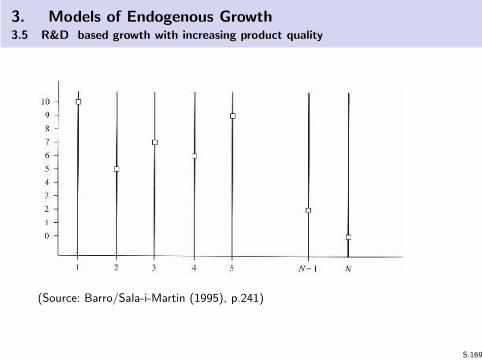
3. Models of Endogenous Growth3.5 R&D based growth with increasing product quality
(Source: Barro/Sala-i-Martin (1995), p.241)
S.169

3. Models of Endogenous Growth3.5 R&D based growth with increasing product quality
(Source: Barro/Sala-i-Martin (1995), p.243)
S.170

3. Models of Endogenous Growth3.5 R&D based growth with increasing product quality
From the quality index to the quality adjusted input of good i :
Index ki = 0, 1, 2, ...
Current quality is qki , that means quality evolves with1, q, q2, ..., qki
A quality adjusted input of an intermediate good i is qkiXi .
S.171

3. Models of Endogenous Growth3.5 R&D based growth with increasing product quality
Final good sector:
Y = N1−αn∑
i=1
[qkiXi ,ki ]α (43)
Firms in the competitive final good sector maximize profits(price normalized to 1):
maxN,Xi
ni=1
π = N1−αn∑
i=1
[qkiXi ,ki ]α − wN −
n∑
i=1
Pi ,kiXi ,ki (44)
where w is the wage and Pi ,ki is the price for input i with qualityki .
S.172

3. Models of Endogenous Growth3.5 R&D based growth with increasing product quality
From FOC we have (similar to the Romer model)
w = (1− α)Y
N(45)
∂Y
∂Xi ,ki
= αN1−αqkiXi ,ki = Pi ,ki (46)
⇒ Xi ,ki = N
(αqki
Pi ,ki
) 11−α
(47)
which is the demand function for intermediate goods. Observe,that without quality improvement (ki = 0) this is the same resultas in the Romer model (equation (41)).
S.173

3. Models of Endogenous Growth3.5 R&D based growth with increasing product quality
Intermediate good sector:
The current quality leader is the monopolist. As in the Romermodel we assume constant marginal cost which are normalized to1. Again, maximization of the profits leads to the optimal price
Pi ,ki =1
α
Employing this price into the demand function yields the optimalinputs of intermediate goods:
Xi ,ki = Nα2
1−α qkiα
1−α
(with ki = 0 this is the same result as in Romer)
S.174

3. Models of Endogenous Growth3.5 R&D based growth with increasing product quality
Substituting Xi ,ki in the production function by its optimal inputlevels leads to
Y = α2α1−αN
n∑
i=1
qkiα
1−α
Let Q be an aggregated quality measure defined as
Q =n∑
i=1
qαki1−α
Then we can write:
Y = α2α1−αNQ
X =n∑
i=1
Xi ,ki = α2
1−αNQ
Since labor force N is constant, it follows
gY = gX = gQS.175

3. Models of Endogenous Growth3.5 R&D based growth with increasing product quality
Profits and present value of the intermediate good firm:
Inserting equilibrium prices and quantities into the profit functionleads to the momentum profits
πi ,ki = N
(1− α
α
)
α2
1−α qkiα
1−α (48)
Recall, that the monopolist earns profits only until a new qualityleader with ki + 1 enters the market. The time duration of themonopoly is therefore
Ti ,ki = tiki+1 − ti ,ki
In equilibrium there will be a constant (= average) interest rate.The present value of the profit flow is then
Vi ,ki =
∫ Ti,ki
0πi ,ki e
−rtdt = πi ,ki ·1− exp(−rTi ,ki )
r
Duration Ti ,ki is unknown and depends on a stochastic innovationprocess! S.176

3. Models of Endogenous Growth3.5 R&D based growth with increasing product quality
Modelling the R&D process:
In this version of the model, the incumbant does not engagein R&D ! He will be replaced by an entrepreneur which is thenew quality leader.
R&D requires a ressource input Zi ,ki (measured in units of Y )of all researchers in sector i .
The probability of achieving a higher quality level ki + 1 (=successful innovation) depends on the input level Zi ,ki :
pi ,ki = Zi ,kiφ(ki ) (49)
where dφ/dki < 0 (since ki is an index number, this is a slightabuse of notation!) denotes that with growing quality =complexity of the product the probability of furtherimprovements decrease.
S.177

3. Models of Endogenous Growth3.5 R&D based growth with increasing product quality
With these assumptions about the stochastic innovationprocess it is possible to determine the expected value of Vi ,ki
(for details see Barro/Sala-i-Martin, chapter 7.2.2):
E [Vi ,ki ] =πi ,ki
r + pi ,ki
The higher the R&D effort of all firms in sector i , the higheris the probability pi ,ki of a successful innovation and the loweris the expected duration of the monopoly (and therefore thepresent value of profits).
We have not yet determined the optimal R&D effort!
S.178

3. Models of Endogenous Growth3.5 R&D based growth with increasing product quality
Incentives for R&D effort:
We assume risk neutrality, i.e. firms respond to the expectedvalue of profits, not to the risk.
There is free market entry. This implies that firms enter themarket as long as there is a positive expected profit. Hence, inequilibrium the zero profit condition must hold true.
pi ,kiE [Vi ,ki+1]− Zi ,ki = 0
pi ,kiπi ,ki+1
r + pi ,ki+1− Zi ,ki = 0 (50)
Rearranging (50) und using (49) leads to
r + pi ,ki+1 = N
(1− α
α
)
α2
1−α · φ(ki ) · qα(ki+1)
1−α (51)
S.179

3. Models of Endogenous Growth3.5 R&D based growth with increasing product quality
To make things more convenient we will now adopt a specificform of φ(·):
φ(ki ) =1
ξ· q
−α(ki+1)
1−α (52)
(Observe the negative dependency on ki ).
Using this specific form of φ(ki ) in the free-entry condition(51) the very last term is cancelled out and we have:
r + p =N
ξ·
(1− α
α
)
α2
1−α (53)
(Observe that p doesn’t depend on ki anymore.)
S.180
3. Models of Endogenous Growth3.5 R&D based growth with increasing product quality
Now we are able to calculate the R&D effort in equilibrium(free-entry condition):
Recall, that the probability of success was defined asp = Zi ,kiφ(ki ).
Solving for Zi ,ki and inserting p from (53) and φ(ki ) from(52) we have
Zi ,ki = qα(ki+1
1−α
(
N
(1− α
α
)
α2
1−α − rξ
)
(54)
and aggregating all R&D expenditures:
Z =n∑
i=1
Zi ,ki = Q · qα
1−α
(
N
(1− α
α
)
α2
1−α − rξ
)
(55)
Hence,gZ = qQ = gY = gX
S.181

3. Models of Endogenous Growth3.5 R&D based growth with increasing product quality
Using (53) for p the expected firm value is
E [Vi ,ki ] = ξ · qαki1−α
and aggregation of all firms leads to
E [V ] = ξ · Q
Therefore, also the expected value of total assets grows with thesame rate:
gV = gQ = gY = gX = gZ
S.182

3. Models of Endogenous Growth3.5 R&D based growth with increasing product quality
Households optimize their present value of utility flow under theintertemporal budget restriction (like in the Romer model).
As we assumed that the intermediate good sector produceswith unit costs, the ressource constraint is given by
C = Y − X − Z
Inserting the calculated expressions for Y ,X ,Z we find thatalso C is proportional to Q, so that gC = gQ .
In absence of population growth the overall growth rate ishence given by the Keynes-Ramsey rule.
S.183

3. Models of Endogenous Growth3.5 R&D based growth with increasing product quality
Optimality:
Since R&D requires patents and monopoly power, the staticefficiency condition price = marginal cost cannot hold true.
Furthermore, there are two externalities: The fact that the entreprenuer’s R&D effort yields an
incremental quality step from ki to ki + 1 implies that healready possess the knowledge how to produce the existingquality ki . This is an external knowledge spillover effect of thepreceeding innovator.
The R&D effort leads to a higher quality index and enhancestherefore the labor productivity in the final good sector.
It is obvious that this creates possibilities of welfare-improvinggovernmental activities (not discussed in this lecture).
S.184

3. Models of Endogenous Growth3.5 R&D based growth with increasing product quality
Extensions (Barro/Sala-i-Martin, chapter 7.4):
Incumbants may also engage in R&D as a monopolyresearcher.
Incumbants as well as outsiders engage in R&D . In this caseit is reasonable to assume that the quality leader has betterinformation about the current quality level and has thereforelower R&D costs.
Further extensions:
Variable (endogenously determined) step size in quality.
Co-existence of quality-leading and older products.
Including imitation as an alternative to innovation.
S.185

3. Models of Endogenous Growth3.6 Technological Progress, Diffusion, and Human Capital
Literature:
Nelson, R.R., Phelps, E.S. (1966), Investment in Humans,Technological Diffusion, and Economic Growth. AmericanEconomic Review 56, 69-75.
Benhabib J., Spiegel, M.M. (2003), Human Capital andTechnology Diffusion. Federal Reserve Bank of San Francisco,Working Paper No. 2003-02.
S.186

3. Models of Endogenous Growth3.6 Technological Progress, Diffusion, and Human Capital
Basic Idea:
Technological progress is exogenous, but diffusion ofinnovation depends on human capital (and may henceendogenously determined).
All previously discussed models assume that new knowledge,new products or better technologies instantanously determinethe production, i.e. there is no diffusion process.
Technology leader = best practice, imitating followers; anincrease in TFP does not neccessarily reflect technologicalprogress, but also improved diffusion of the best practicetechnology.
Regional models of growth (“North-South” models,leader-follower structures)
S.187

3. Models of Endogenous Growth3.6 Technological Progress, Diffusion, and Human Capital
Here: Human Capital plays not a role as a production factor.
HC is needed to absorb the knowledge about newtechnologies, and to employ new technologies in theproduction process.
The diffusion or “catching up” process is therefore notcostless (as in previously discussed models), but it depends onHC investment.
This mechanism could also be applied to an endogenousgrowth framework: Adoption or imitation cost of the followercreate an incentive to innovate (as an alternative mechanismto patenting and monopoly power).
S.188

3. Models of Endogenous Growth3.6 Technological Progress, Diffusion, and Human Capital
The Approach of Nelson/Phelps:
Exogenous Harrod neutral technological progress:
Y (t) = F (K (t),A(t) · N(t))
where A is the “average” TFP index.
Best-practice level of technology (technology frontier) evolvesaccording to
T (t) = T0 · eλt , λ > 0
S.189

3. Models of Endogenous Growth3.6 Technological Progress, Diffusion, and Human Capital
Diffusion process:
A(t) = φ(h)(T (t)− A(t))
gA =A
A= φ(h)
(T (t)− A(t)
A(t)
)
(56)
where the bracket term is the “technology gap”.
The term φ(h) with dφ/dh > 0 denotes the strength of thecatching-up dynmic whch depends on human capital h.
The average TFP grows faster in case of a large technologygap, and becomes zero when the gap declines to zero.
Since the frontier technology T grows with the rate λ, thegap will never be closed.
S.190

3. Models of Endogenous Growth3.6 Technological Progress, Diffusion, and Human Capital
T−AA
λφ(h)
TT
AA
λ
S.191

3. Models of Endogenous Growth3.6 Technological Progress, Diffusion, and Human Capital
In equilibrium the gap is
T − A
A=
λ
φ(h)(57)
In a stagnating economy λ = 0 the gap will be closed in finitetime.
Differentiating (57) with respect to h an rearranging leads to
dA
dh·h
A=
(hφ′(h)
φ(h)
)(λ
φ(h) + λ
)
The effect of an increased education on the TFP is higher themore technologically progressive the economy is (λ)
S.192

3. Models of Endogenous Growth3.6 Technological Progress, Diffusion, and Human Capital
(Source: Benhabib/Spiegel)
S.193

3. Models of Endogenous Growth3.6 Technological Progress, Diffusion, and Human Capital
The Benhabib/Spiegel approach:
Modification of the Nelson/Phelps model.
Innovative country “North” develops the technology frontier,imitating country “South” is catching up.
Variant A:
AN
AN
= g(HN) (58)
AS
AS
= g(HS) + c(HS)
(AN
AS
− 1
)
(59)
with g(·), c(·) as increasing functions.
It is g(Hi ) the base rate of technical progress where the North isendowed with more human capital (HN > HS) and henceforthg(HN) > g(HS). In the starting point there is AN > AS .
c(HS)(AN/AS − 1) like in Nelson/Phelps approach.S.194

3. Models of Endogenous Growth3.6 Technological Progress, Diffusion, and Human Capital
Let HN ,HS be constant (ceteris paribus), and thereforegN = g(HN), gS = g(HS), cS = c(HS).
The solution of the differential equation (59) is given by
AS(t) = (AS(0)− ΩAN(0))e(gS−cS )t +ΩAN(0)e
gN t
withΩ =
cScS − gS + gN
> 0
It can be shown that (similar to the Nelson/Phelps approach)there is a balanced growth path with
limt→∞
AS(t)
AN(t)= Ω
(constant relative distance in TFP)
S.195

3. Models of Endogenous Growth3.6 Technological Progress, Diffusion, and Human Capital
Variant B:
In the economics of innovation a broadly used concept is alogistic diffusion process:
The catching-up dynamic is modest when the technology gapis large, it accelerates with a declining gap, and it slows downagain when the technology gap becomes small: We replace(59) by
AS
AS
= g(HS) + c(HS)
(AS
AN
)(AN
AS
− 1
)
(60)
This damps the dynamic in case of small values of AS .
It may be the case that the South fails to catch up if theSouth is very low endowed with human capital.
S.196

3. Models of Endogenous Growth3.6 Technological Progress, Diffusion, and Human Capital
The following result could be derived:
limt→∞
AS(t)
AN(t)=
cS−gs+gNcS
if cS + gS − gN > 0AS (0)AN(0)
if cS + gS − gN = 0
0 if cS + gS − gN < 0
The last case describes a poorly HC endowed South withcS + gS < gN so that the technology gap becomes infinitelylarge.
⇒ “convergence clubs” or “poverty trap” (see stylized facts)
S.197

3. Models of Endogenous Growth3.6 Technological Progress, Diffusion, and Human Capital
Some empirical evidence:
Teles, V.K. (2005), The Role of Human Capital in EconomicGrowth. Applied Economics Letters 12, 583-587.
The Lucas model “satisfactorily explains” the human capitalbased endogenous growth in rich countries, but cannot explainthe fact of convergence clubs or poverty traps.
Nelson/Phelps type models could explain poverty traps but donot properly describe the growth process in rich countries.
S.198

3. Models of Endogenous Growth3.7 Further Issues
1) North-South models of regional growth(Aghion/Howitt (2009), chapter 7; Barro/Sala-i-Martin (1995), chapter
8)
technological catch-up processes, cross-country convergence
“leapfrogging” processes
2) Growth in open economies(Aghion/Howitt (2009), chapter 15)
Role of trade
Role of factor mobility (capital flow, migration)
Brain Drain
S.199

3. Models of Endogenous Growth3.7 Further Issues
3) The Role of Financial Markets and Financial Institutionsfor Growth(Aghion/Howitt (2009), chapter 6)
Credit constraints for financing investments (marketimperfections)
Financial Intermediates/Institutions as a prerequisite forgrowth
Finance-led growth vs. slow-down by financialisation
S.200

3. Models of Endogenous Growth3.7 Further Issues
4) Implications of Intellectual Property Rights (IPR) regimes(O’Donoghue, T., Zweimuller, J. (2004), Patents in a Model of EndogenousGrowth. Journal of Economic Growth 9, 81-123;Scotchmer, S. (1991), Standing on the Shoulders of Giants: CumulativeResearch and the Patent Law. Journal of Economic Perspectives 5, 29-41;Falvey, R., Foster, N., Greenaway, D. (2006), Intellectual Property Rights andEconomic Growth. Review of Development Economics 10(4), 700–719;Horii R., Iwaisako T.(2007), Economic Growth with Imperfect Protection ofIntellectual Property Rights. Journal of Economics 90(1), 45–85;Papers from Boldrin/Levine, Lerner, and Mokyr in American Economic Review.
Papers and Proceedings 99(2), 2009, 337-355;
Koleda, G. (2008), Promoting innovation and competition with patent policy.
Journal of Evolutionary Economics 18, 433-453.)
IPR are needed to stimulate incentives for R&D On the other hand they constrain knowledge diffusion and
cumulative knowledge creation Optimal design of IPR, depending on technology and
institutions Open Source, Open Access, Open Innovation S.201

3. Models of Endogenous Growth3.7 Further Issues
5) Growth models with directed technological progress andstructural change(Aghion/Howitt (2009), chapter 8)
Innovation activities are heterogeneous, depending on marketsize
6) Growth models with Overlapping GenerationsDiamond, P. (1965), National Debt in a Neoclassical Growth Model.
American Economic Review 55(1), 1126-1150.
7) Stochastic Growth Models(Acemoglu (2008), chapter 5, Aghion/Howitt (2009), chapter 14)
S.202

3. Models of Endogenous Growth3.7 Further Issues
8) Institutions and Growth(Aghion/Howitt (2009), chapter 11, 17)
Role of stable political institutions
Role of corruption
Role of Economic Freedom and Democracy
Cultural Issues
9) Growth and Environment
Ressource constrained growth
Growth and pollution (ecological externalities)
S.203

3. Models of Endogenous Growth3.7 Further Issues
10) Growth and Distribution(Bertola, G., Foellini, R., Zweimuller, J. (2005), Distribution inMacroeconomic Models. Princeton University Press,
Perotti, R. (1996), Growth, Income Distribution, and Democracy: What
the Data Say. Journal of Economic Growth 1, 149-187.
Effects of Growth on Distribution and vice versa
Is inequality “good” or “bad” for growth?
Distribution of Income, distribution of assets
11) Growth Policy (Aghion/Howitt (2009), part III)
Lessons from “New” Endogenous Growth Theory
S.204

3. Models of Endogenous Growth3.7 Further Issues
12) Non-mainstream approaches to growth theory:
(Post-) Keynesian Approaches
Evolutionary Approaches (see section 4)
S.205

4. Critique and an Evolutionary Perspective4.1 Empirical Evidence
Broad empiricial growth literature = growth regressions(see chapter 13. - 1.4)
Growth rates are linked to (“explained by”) severaldeterminants which play a role in modern endogenous growththeories (investment, human capital, R&D etc.).
Some links are more or less robust, others not. Some convergence results are in line with theory, others not.
Especially the emergence of convergence clubs and largeregional disparities are not satisfyingly explained.
Country specific determinants, different policies, andinstitutional issues seem to play a significant role, which is notreflected in most endogenous growth models.
It is a difference whether a “stylized fact” of a model is compatiblewith empirical findings, or if the model itself is econometricallyestimated, and the predictions of the estimated models work well!
S.206
4. Critique and an Evolutionary Perspective4.1 Empirical Evidence
Durlauf, S.N., Kourtellos, A., Tan, C.M. (2008), Are Any GrowthTheories Robust? The Economic Journal 118, 329–346.
“[We] find little evidence that so-called fundamental growththeories play an important role in explaining aggregate growth. Incontrast, we find strong evidence for macroeconomic policy effectsand a role for unexplained regional heterogeneity, as well as someevidence of parameter heterogeneity in the aggregate productionfunction. We conclude that the ability of cross-country growthregressions to adjudicate the relative importance of alternativegrowth theories is limited.”
S.207

4. Critique and an Evolutionary Perspective4.1 Empirical Evidence
Capolupo, R. (2009), The New Growth Theories and TheirEmpirics after Twenty Years Economics: The Open-Access,Open-Assessment E-Journal Vol. 3, 2009-1
“The author [...] argues that: (i) causal inference drawn from theempirical growth literature remains highly questionable, (ii) thereare estimates for a wide range of potential factors but theirmagnitude and robustness are still under debate.”
In order to let endogenous growth theory not to lose out toomuch...
“Her conclusion, however, is that, if properly interpreted, thepredictions of endogenous growth models are gathering increasingempirical support.”
S.208

4. Critique and an Evolutionary Perspective4.1 Empirical Evidence
Parente, S.L. (2000), The Failure of Endogenous Growth.Knowledge, Technology and Policy 13(4), 49-58
“My own assessment is that this line of research has not provenuseful for understanding the most important question faced byeconomists today, namely, why isn’t the whole world rich.Exogenous growth theory, in contrast, is. Endogenous growth mayprove useful for understanding growth in world knowledge overtime, but it is not useful for understanding why some countries areso poor relative to the United States today.”
S.209

4. Critique and an Evolutionary Perspective4.2 Methodological Objections
Endogenous growth theory has a rigorous methodological basewhich is broadly accepted in mainstream economics andsometimes considered as a “prerequisite” for economicreasoning.
representative agents intertemporal optimization perfect markets, existing complete future markets general equilibrium for all t etc.
Without doubt, it has shed light on the determinants andmechanisms of economic growth.
The question arises whether the little plus of explanatorypower compared to exogenous growth models is worth theprice of high artificiality (if not counterfactuality) ofassumptions, and of mathematical effort.
S.210
4. Critique and an Evolutionary Perspective4.2 Methodological Objections
Solow, R.M. (2007), The last 50 years in growth theory and thenext 10. Oxford Review of Economic Policy 23(1), 3–14.
“I suspect that the most valuable contribution of endogenous growththeory has not been the theory itself, but rather the stimulus it hasprovided to thinking about the actual ’production’ of human capital anduseful technological knowledge.”
“Instead, the main argument for this modelling strategy has been a moreaesthetic one: its virtue is said to be that it is compatible with generalequilibrium theory, and thus it is superior to ad hoc descriptive modelsthat are not related to ‘deep’ structural parameters. The preferrednickname for this class of models is ‘DSGE’ (dynamic stochastic generalequilibrium). I think that this argument is fundamentally misconceived.”
“The cover story about ‘micro-foundations’ can in no way justify recourseto the narrow representative-agent construct. Many other versions of theneoclassical growth model can meet the required conditions; it is onlynecessary to impose them directly on the relevant building blocks.”
S.211

4. Critique and an Evolutionary Perspective4.2 Methodological Objections
Some methodological objections in more details:
Perfect Rationality, Intertemporal Optimization
Robust empirical and experimental evidence against“economic model of man” A positive (explanatory) growththeory must have a less rigorous understanding ofmicrofoundation Moreover: Is it really neccessary for amacroeconomic theory to be “microfounded”?
Arrow-Debreu Economy, Walrasian Equilibrium
This is an artificial economy for normative theoreticalinvestigations only (e.g. to prove the existence and stability ofgeneral equilibria). It is not clear why this should be the basisfor an explanatory positive theory.
S.212

4. Critique and an Evolutionary Perspective4.2 Methodological Objections
Equilibrium growth paths rather than disequilibrium motion
Endogenous growth models operate on equilibrium paths only.By principle it is not possible to analyze what happens indisequilibrium situations. This view is in strong contradictionto an evolutionary perspective.
So-called “Schumpetarian” models with “creativedestruction” on an Walrasian equailibrium path is a very highquestionable concept!
Alcouffe A., Kuhn, T. (2004), Schumpeterian endogenousgrowth theory and evolutionary economics. Journal ofEvolutionary Economics 14, 223–236.
“We find endogenous growth theory far from carryingSchumpeter’s idea of an evolutionary approach to change anddevelopment.”
S.213

4. Critique and an Evolutionary Perspective4.3 Evolutionary Approaches: Outline
However, endogenous growth theories claim to describe R&D ,innovation activities, and “Schumpeterian” processes of“creative destruction” – these are features of evolutionarytheorizing!
However, despite such semantic similarities there existfundamentally different styles of economic reasoning:
Castellacci, F. (2007), Evolutionary and New GrowthTheories. Are They Converging? Journal of Economic Surveys21(3), 585-627.
Alcouffe A., Kuhn, T. (2004), Schumpeterian endogenousgrowth theory and evolutionary economics. Journal ofEvolutionary Economics 14, 223–236.
S.214

4. Critique and an Evolutionary Perspective4.3 Evolutionary Approaches: Outline
Very stylized comparison:
orthodox evolutionaryparadigm paradigm
agent representative agent heterogenous agentsrationality unbounded bounded (e.g. heuristic,
adaptive behavior)expectations rational different expectation
hypothesis (e.g. adaptive)dynamic state Walrasian equilibrium generation of disequilibria,
diffusion processes,equilibrating processes
model solution equilibrium analysis simulation analysis
S.215

4. Critique and an Evolutionary Perspective4.4 Evolutionary Approaches: Example
Dosi, G., Fagiolo, G., Roventini, A. (2008), Schumpeter Meeting Keynes:A Policy-Friendly Model of Endogenous Growth and Business Cycles.LEM Working Paper series No.2008/21.
Main issues:
Discrete time concept
Sectors: Capital good production, consumption godd production,households, government
In both production sectors: heterogenous firms, free entry and exit,development of market shares
Capital good sector: Stochastic R&D with innovation and imitation
Consumption good sector: Diffusion of new technologies
Heuristic behavior, adaprtive expectations, imperfect information
Disequilibrium features like unexpected inventory changes, creditrationing, and unemployment
Government activities: Taxing and paying unemployment grants
S.216

4. Critique and an Evolutionary Perspective4.4 Evolutionary Approaches: Example
We will not analyze the model in detail! Only sketch of thestructure.
Many “realistic” features = no analytic solutions, noanalytical results, but numerical simulations
Role of robustness
By numerical experiments it is possible to determine whichfeatures/assumptions are crucially driving the pattern ofevolution.
By numerical experiments it is possible to explore the impactof different policies.
S.217

4. Critique and an Evolutionary Perspective4.4 Evolutionary Approaches: Example
Households
labor supplyconsumption
labor labor
consumptiongoods
entry exitentryexit
Capital good sector Consumption good sector
government
tax taxtax unemployment
grants
capital
goods
S.218

4. Critique and an Evolutionary Perspective4.4 Evolutionary Approaches: Example
Timing of events:
Capital good firms decide on R&D (innovation, costly imitation) tocreate more efficient machines.
Capital good firms advertise their machines to consumption goodfirms.
Consumption good firms decide on investment and production(based on demand expectations). If investment is positive, theychoose their capital good supplier on the basis of advertisementsand order machines.
Both sectors decide on the employed worker (and implicetly aboutunemployment)
Consumption good markets opens. The market shares developaccording to the price competitiveness.
In both sectos entries and exits take place according to marketshares and the amount of liquid assets.
Ordered machines are delivered and are part of the capital stock int + 1 (vintage capital). S.219

4. Critique and an Evolutionary Perspective4.4 Evolutionary Approaches: Example
Capital good industry (firm index i):
Efficiency is measured by labor productivity Bτi for capital
good firms and Aτi for consumption good firms which use the
technology from capital good firm i (it is τ the currenttechnological level).
Unit cost of production : ci (t) = w(t)/Bτi .
Markup pricing: pi (t) = (1 + µ1)ci (t)
S.220

4. Critique and an Evolutionary Perspective4.4 Evolutionary Approaches: Example
R&D activities and innovation:
A constant fraction ν ∈ (0, 1) of past sales is spent for R&D :RDi (t) = νSi (t − 1)
R&D effort is split to innovation and imitation effort:
INi (t) = ξRDi (t)
IMi (t) = (1− ξ)RDi (t)
Probability, that innovation effort has a result:
θINi (t) = 1− exp(−ξ1INi (t))
S.221

4. Critique and an Evolutionary Perspective4.4 Evolutionary Approaches: Example
The result of innovation is captured by its effect on the laborproductivity:
AINi (t) = Ai (t)(1 + xAi (t))
B INi (t) = Bi (t)(1 + xBi (t))
where x ji are random variables taken independently from a Betadistribution over the intervall [−a,+b] (the technologicalopportunities). Only positive values denote a technologicalprogress. Negative values means that the innovation is “worse”and will not be implemented.
S.222

4. Critique and an Evolutionary Perspective4.4 Evolutionary Approaches: Example
Imitation also proceeds in two steps: The probability that a firmhas the chance to imitate is given by
θIMi (t) = 1− exp(−ξ2INi (t))
If a firm imitates, it is more likely that the firm imitates acompetitor with a “similar” technology (measured by a metric oftechnological distance).
S.223

4. Critique and an Evolutionary Perspective4.4 Evolutionary Approaches: Example
Finally, the firm decides whether to produce capital goods(machines) of the current technological level τ , the imitatedtechnology IM or the new technology IN (innovation).
The firm sends “brochures” to the former clients and to arandom sample of new clients from the consumption goodindustry (providing the information of the new technologicallevel imperfectly to the customer market)
S.224

4. Critique and an Evolutionary Perspective4.4 Evolutionary Approaches: Example
The Consumption Good Industry (firm index j)
The firm has extrapolative (“adaptive”) demand expectations
Dj(t)e = f (Dj(t − 1),Dj(t − 2), ...)
The desired level of production is
Qdj (t) = De
j (t) + Ndj (t)− Nj(t − 1)
where N(Nd) is the (desired) level of inventory, and Nd is afraction of De
j .
This desired output level is constrained by the possibility to hireworkers as well as by the capital stock. The desired capital stockK d(t) is a function of the desired output.
Investments are hence
Edj (t) = K d
j (t)− Kj(t)
S.225

4. Critique and an Evolutionary Perspective4.4 Evolutionary Approaches: Example
The capital stock is composed of capital goods from differentvintages (and therefore technological levels τ).
Instead of constant depreciation of a homogenous capital stock, thefirm decides on scrapping machines and replacing them by newmachines of the current vintage. This is done by a routine: Allmachine with Aτ
j which are “technologically obsolescent” arereplaced:
RSj(t) =
Aτj with
p∗
c(Aτt )− c∗
≤ z
where p∗ is the price of the new machine and c∗ as the unit costs ofproduction when using the new machine.
The new machines are chosen from the “brochures” sent by thecapital good firms. From this imperfect knowledge about thecurrent technological state they choose the machines whichbalances machine price and unit cost of production optimally.
Together with the desired investment volume E dj (t) the machine
order is complete and announced to capital good firm i .S.226

4. Critique and an Evolutionary Perspective4.4 Evolutionary Approaches: Example
Firms have to finance the investment expenditures as well asthe employed workers.
They will use internal sources (liquid assets or net worth)NWj(t). If this is not sufficient to finance desired output andinvestment, they will borrow money at the credit market withan interest rate r up to a given debt/sales ratio.
It may be the case that due to credit market imperfections thecredit demand is rationed. Then, of course, the productionand investment plans have to be cut.
S.227

4. Critique and an Evolutionary Perspective4.4 Evolutionary Approaches: Example
Consumption good prices are determined by a variable markuprule:
pj(t) = (1 + µ2(t))cj(t)
where the markup evolves according to the market power(“market shares”):
µj(t) = µj(t − 1)
(
1 + vfj(t − 1)− fj(t − 2)
fj(t − 2)
)
where fj denotes the market power.
The market power depends on the competitiveness which is afunction of the price and the ability to deliver goods whenthey are demanded.
The “market shares” evolve according to the relativecompetitiveness (similar to replicator dynamics).
S.228

4. Critique and an Evolutionary Perspective4.4 Evolutionary Approaches: Example
The resulting profits of the consumption good firm is given by
Πj(t) = pj(t)Dj(t)− cj(t)Qj(t)− r · Debj(t)
where Deb is the “stock debt”
The liquid assets (net wealth) are given by
NWj(t) = NWj(t − 1) + Πj(t)− cIc(t)
where cIc are the internal funds for financing investment.
S.229

4. Critique and an Evolutionary Perspective4.4 Evolutionary Approaches: Example
Entry and Exit Dynamics:
In each t firms with almost zero market shares or negative netassets have to leave the market.
They are replaced by new firms, so that the number of firms isconstant.
The technology of new firms is determined by a probabilitydistribution of “technological draws” from the set of“brochures”.
S.230

4. Critique and an Evolutionary Perspective4.4 Evolutionary Approaches: Example
Labor Market:
The market is not Walrasian, i.e. unemployment may takeplace.
Labor supply LS is unelastic and given.
Labor demand LD is the sum of labor demand in capital goodand consumption good industry, determined by their outputdecisions.
The wages adapt according changes in the price level, theunemployment rates, and the labor productivity.
S.231

4. Critique and an Evolutionary Perspective4.4 Evolutionary Approaches: Example
Consumption, Taxes, and Public Expenditures:
If a worker is unemployed, he receives a grant which is aconstant fraction of the market wage:
wu(t) = φw(t), φ ∈ (0, 1)
We have the “classical saving hypothesis” that household(labor income only) do not save, and savings result fromcapital income where capital is owned by the firms. Hence,
C (t) = w(t)LD(t) + wu(t)(LS − LD(t))
The total income from production of consumption, capitalgoods and inventory change (∆N) ist
∑
i
Qi (t) +∑
j
Qj(t) = Y (t) = C (t) + I (t) + ∆N(t)
S.232

4. Critique and an Evolutionary Perspective4.4 Evolutionary Approaches: Example
It makes no sense to try to construct from these formulas asystem of difference euqations (stochastic, nonlinearities).
Note, that we have heterogenous firms with entry and exitdynamics (a difference equation must then average of thefirms).
The model is analysed by simulation studies.
Before doing that, all parameters have to be calibrated: Thevalues are set in a way that the resulting dynamic is similar tothe empirically observed patterns on a micro and macro level.
Then it is possible to make polcy experiments: How do thedynamic respond to different adjustments of policy variables?
S.233

4. Critique and an Evolutionary Perspective4.4 Evolutionary Approaches: Example
Reproduced stylized facts:
Macro level:
The model produces endogenous self-sustained growth withpersistent fluctuations. Consumption and investmentsfluctuate procyclical while the latter has a larger volatility andconsumption a lower volatility than the output.
Productivity, inflation, and markups are procyclical.
Distribution of growth rates has fat tails.
(Not mentioned in the paper: With constant Ls , growing Yand positive net investments we have per capita growth andgrowing capital intensity)
S.234

4. Critique and an Evolutionary Perspective4.4 Evolutionary Approaches: Example
Micro level:
The distribution of firm (log) sizes is skewed and notlog-normal.
Productivity differentials of firms persists over time.
There is lumpiness in investment (co-existence of firms withalmost zero investment and firm with investment peaks).
S.235

4. Critique and an Evolutionary Perspective4.4 Evolutionary Approaches: Example
Policy experiments:
“Schumpeterian side” of the model is related to the innovation activities.“Keynesian side” of the model is related to governmental acrivities.
Enlargeing the innovation opportunities (the support of the Betadistribution of innovation outcomes): Higher opportunities have apositive impact on growth rate, reduce unemployment, slightincrease in GDP volatility.
Enlarging search capabilities (the ξ1, ξ2 in the Bernoullidistribution): With a higher probability that R&D effort leads to aninnovation (no matter if successful or not) leads to higher growthrates, lower unemployment and lower volatility.
Approprability of Innovation Output: R&D could be invested eitherin innovation or imitation. Better approprability menas lessimitation, i.e. the patent length determines the number of periodswhere imitation could not take place. Increasing patent lengthlowers the growth rate and increases unemployment.
S.236

4. Critique and an Evolutionary Perspective4.4 Evolutionary Approaches: Example
Easyness of entry and exit (entry barriers are captured by theprobability distribution of “technological draws”): If the entryis easier, then the growth rate is higher and unemploymentlower.
Competitiveness: Higher competition is reflected by a moreeffective replicator dynamic. Higher competitiveness has nosignificant effect on the growth rate, but it lowersunemployment and reduces volatility.
If we abandon the Keynesian side (turn off governmentalactivities), the growth rate slows down significantly,unemployment shoots up, and volatility increases. This holdsalso true also in the case of large Schumpetarian dynamics(large innovation opportunities etc.).
It seems to be the case that there can be “too less”governmental economic activities, but not “too much”.
S.237

4. Critique and an Evolutionary Perspective4.4 Evolutionary Approaches: Example
Concluding Remarks:
“Microfoundadtion”: Deriving behavior from a closed calculusvs. heuristic behavioral assumptions with high descriptiverelevance – how to judge the explanatory power?
Steady state analysis vs. simulation experiments – how tojudge the explanatory power?
Equilibrium movements vs. Non-Walrasian adaption – how tojudge the explanatory power?
S.238


![The 5 Levels of Platform Growth [Slides]](https://static.fdocuments.in/doc/165x107/554cf669b4c905ae138b4f50/the-5-levels-of-platform-growth-slides.jpg)

![Week 9 slides growth&business cycle [core]](https://static.fdocuments.in/doc/165x107/54bf9e084a7959d1158b468b/week-9-slides-growthbusiness-cycle-core.jpg)


![[Slides] Keys to Community Readiness and Growth Study](https://static.fdocuments.in/doc/165x107/588310c31a28ab31068b5659/slides-keys-to-community-readiness-and-growth-study.jpg)

