Slides for Chapter 3: The basic closed-economy …markusen/teaching_files/...2 (4) Equilibrium...
86
1 Slides for Chapter 3: The basic closed-economy general- equilibrium model as an MCP Copyright: James R. Markusen University of Colorado, Boulder 1. Introduction to applied general-equilibrium modeling (1) Multiple interacting agents (2) Individual behavior based on optimization (3) Most agent interactions are mediated by markets and prices
Transcript of Slides for Chapter 3: The basic closed-economy …markusen/teaching_files/...2 (4) Equilibrium...
1
Slides for Chapter 3: The basic closed-economy general-equilibrium model as an MCP
Copyright: James R. Markusen University of Colorado, Boulder
1. Introduction to applied general-equilibrium modeling
(1) Multiple interacting agents
(2) Individual behavior based on optimization
(3) Most agent interactions are mediated by markets and prices
2
(4) Equilibrium occurs when endogenous variables (e.g., prices)adjust such that
(a) agents, subject to the constraints they face, cannot dobetter by altering their behavior
(b) markets (generally, not always) clear so, for example,supply equals demand in each market.
2. Steps in Applied General-Equilibrium Modeling
(1) Specify dimensions of the model.• Numbers of goods and factors• Numbers of consumers• Numbers of countries• Numbers of active markets
3
(2) Chose functional forms for production, transformation, and utility functions; specification of side constraints.
• Includes choice of outputs and inputs for each activity• Includes specification of initially slack activities
(3) Construct micro-consistent data set.• Data satisfies zero profits for all activities, or if profits are
positive, assignment of revenues• Data satisfies market clearing for all markets
(4) Calibration – parameters are chosen such that functional formsand data are consistent.
• By “consistent”: data represent a solution to the model
(5) Replication – run model to see if it reproduces the input data.
(6) Counter-factual experiments.
4
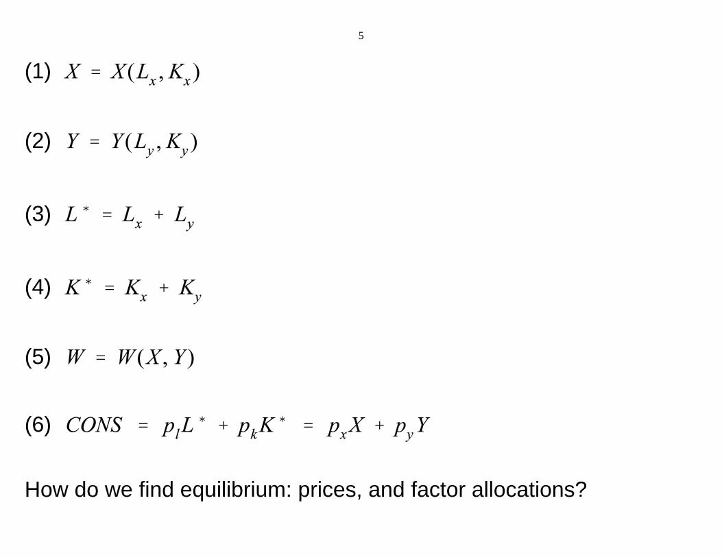
Example M3-4a: 2-good, 2-factor closed economy with fixedfactor endowments, one representativeconsumer.
Simply economy, two sectors (X and Y), two factors (L and K), andone representative consumer (utility function W).
L and K are in inelastic (fixed) supply, but can move freely betweensectors.
px, py, pl, and pk are the prices of X, Y, L and K, respectively.
CONS is consumer’s income and pw will be used later to denote theprice of one unit of W.
5
(1)
(2)
(3)
(4)
(5)
(6)
How do we find equilibrium: prices, and factor allocations?
6
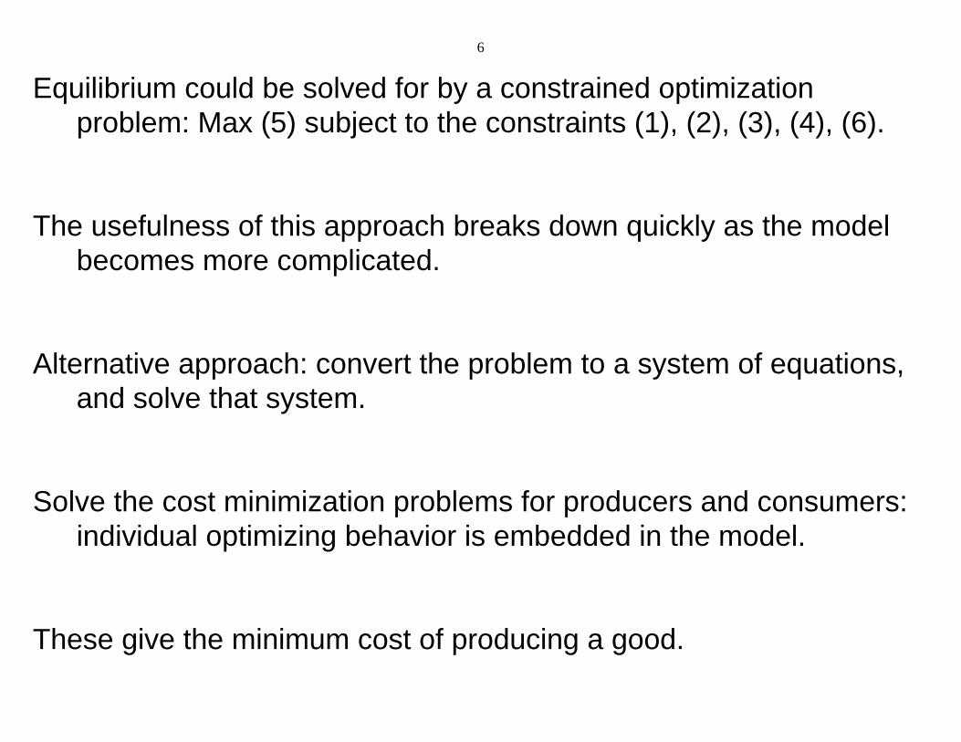
Equilibrium could be solved for by a constrained optimizationproblem: Max (5) subject to the constraints (1), (2), (3), (4), (6).
The usefulness of this approach breaks down quickly as the modelbecomes more complicated.
Alternative approach: convert the problem to a system of equations,and solve that system.
Solve the cost minimization problems for producers and consumers:individual optimizing behavior is embedded in the model.
These give the minimum cost of producing a good.
7
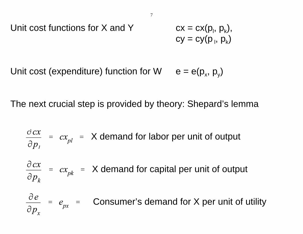
Unit cost functions for X and Y cx = cx(pl, pk), cy = cy(p l, pk)
Unit cost (expenditure) function for W e = e(px, py)
The next crucial step is provided by theory: Shepard’s lemma
X demand for labor per unit of output
X demand for capital per unit of output
Consumer’s demand for X per unit of utility
8
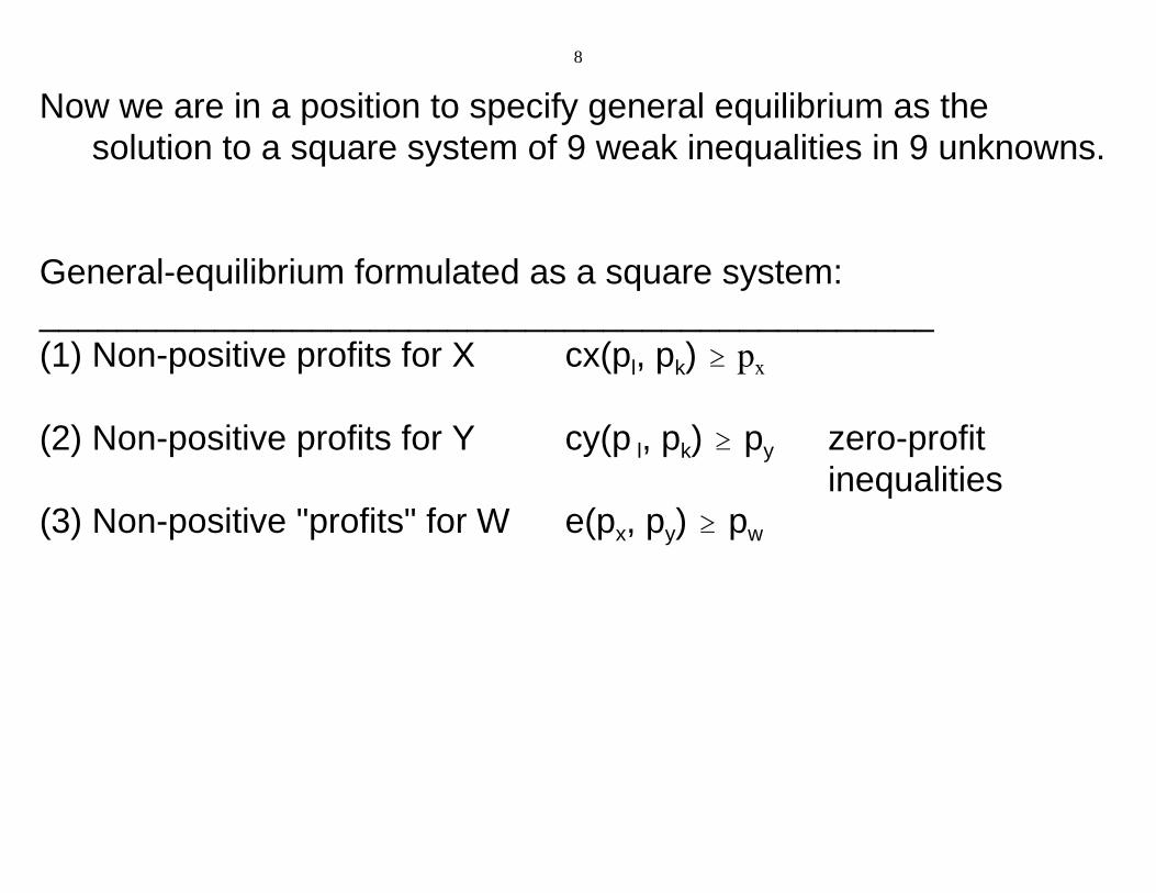
Now we are in a position to specify general equilibrium as thesolution to a square system of 9 weak inequalities in 9 unknowns.
General-equilibrium formulated as a square system:______________________________________________(1) Non-positive profits for X cx(pl, pk) $ px
(2) Non-positive profits for Y cy(p l, pk) $ py zero-profit
inequalities(3) Non-positive "profits" for W e(px, py) $ pw
9
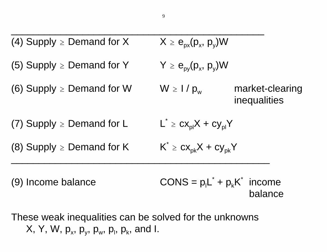
______________________________________________(4) Supply $ Demand for X X $ epx(px, py)W
(5) Supply $ Demand for Y Y $ epy(px, py)W
(6) Supply $ Demand for W W $ I / pw market-clearinginequalities
(7) Supply $ Demand for L L* $ cxplX + cyplY
(8) Supply $ Demand for K K* $ cxpkX + cypkY_______________________________________________
(9) Income balance CONS = plL* + pkK* incomebalance
These weak inequalities can be solved for the unknownsX, Y, W, px, py, pw, pl, pk, and I.
10
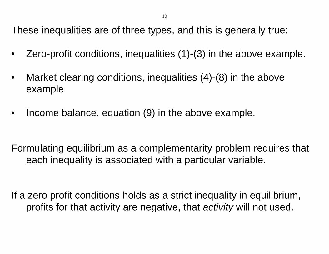
These inequalities are of three types, and this is generally true:
• Zero-profit conditions, inequalities (1)-(3) in the above example.
• Market clearing conditions, inequalities (4)-(8) in the aboveexample
• Income balance, equation (9) in the above example.
Formulating equilibrium as a complementarity problem requires thateach inequality is associated with a particular variable.
If a zero profit conditions holds as a strict inequality in equilibrium,profits for that activity are negative, that activity will not used.
11
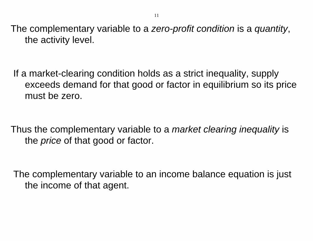
The complementary variable to a zero-profit condition is a quantity,the activity level.
If a market-clearing condition holds as a strict inequality, supplyexceeds demand for that good or factor in equilibrium so its pricemust be zero.
Thus the complementary variable to a market clearing inequality isthe price of that good or factor.
The complementary variable to an income balance equation is justthe income of that agent.
12
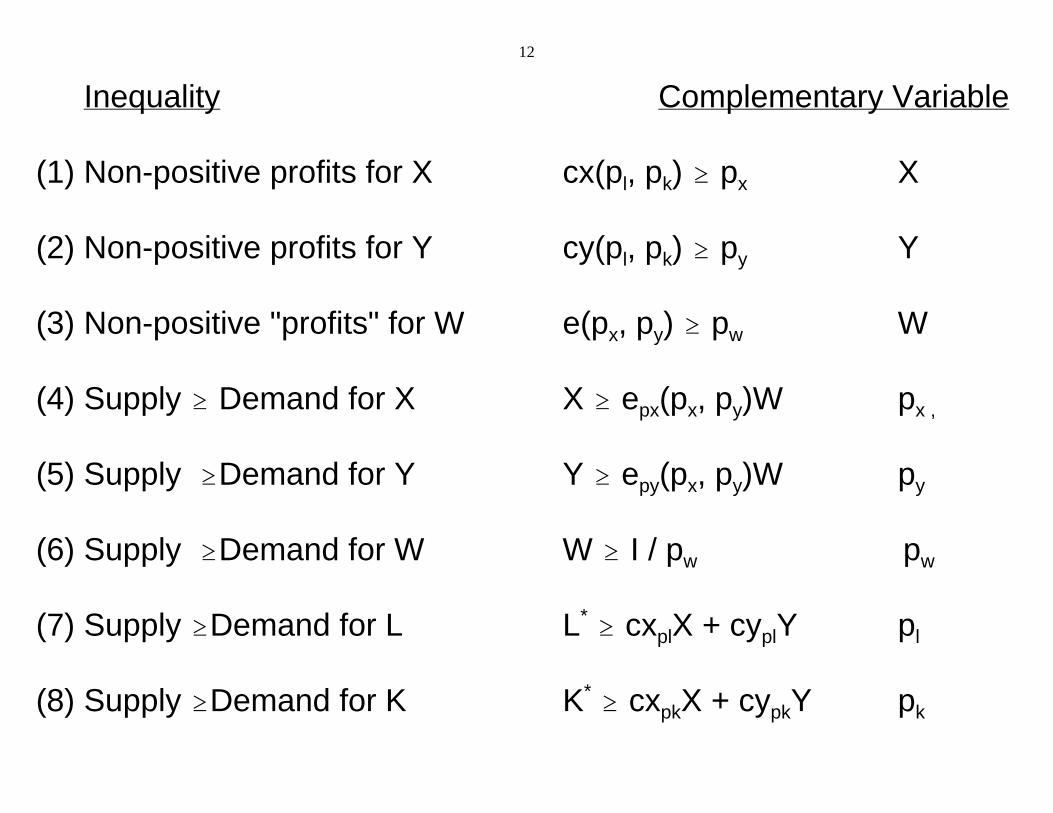
Inequality Complementary Variable
(1) Non-positive profits for X cx(pl, pk) $ px X (2) Non-positive profits for Y cy(pl, pk) $ py Y
(3) Non-positive "profits" for W e(px, py) $ pw W
(4) Supply $ Demand for X X $ epx(px, py)W px ,
(5) Supply $Demand for Y Y $ epy(px, py)W py
(6) Supply $Demand for W W $ I / pw pw
(7) Supply $Demand for L L* $ cxplX + cyplY pl
(8) Supply $Demand for K K* $ cxpkX + cypkY pk
13
(9) Income balance CONS = plL* + pkK* CONS
3.2 Micro consistent data
A data set is micro consistent when it satisfies the conditions foreconomic equilibrium (it could be generated as the solution tosome model).
Data must satisfy zero profits, market clearing, and income balance.
The above problems can be thought of as consisting of three production activities, X, Y, and W, four markets, X, Y, L, and Kincome balance
14
Represent the initial data for this economy by a rectangular matrix. This matrix is related to the concept of a “SAM” – socialaccounting matrix
There are two types of columns in the rectangular matrix,corresponding to production activities(sectors) and consumers.
In the model outlined above, there are three production sectors (X, Yand W) and a single consumer (CONS).
Rows correspond to markets. Complementary variables are prices,so we have listed the price variables on the left to designate rows.
15
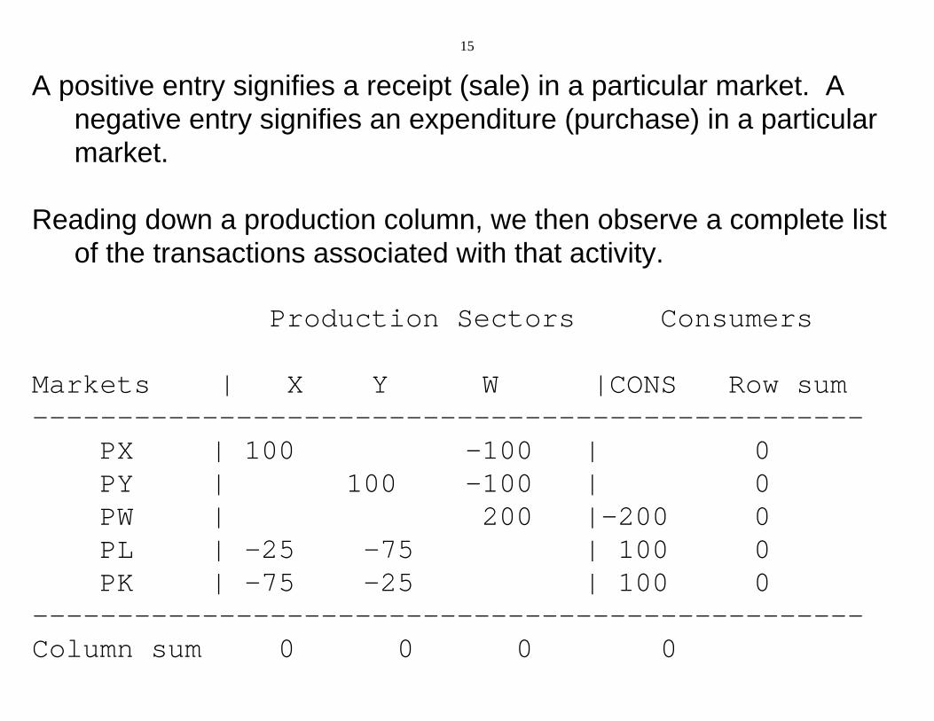
A positive entry signifies a receipt (sale) in a particular market. Anegative entry signifies an expenditure (purchase) in a particularmarket.
Reading down a production column, we then observe a complete listof the transactions associated with that activity.
Production Sectors Consumers
Markets | X Y W |CONS Row sum------------------------------------------------- PX | 100 -100 | 0 PY | 100 -100 | 0 PW | 200 |-200 0 PL | -25 -75 | 100 0 PK | -75 -25 | 100 0-------------------------------------------------Column sum 0 0 0 0
16
A rectangular SAM is balanced or “micro-consistent” when row andcolumn sums are zeros.
Positive numbers represent the value of commodity flows into theeconomy (sales or factor supplies),
Negative numbers represent the value of commodity flows out of theeconomy (factor demands or final demands).
A row sum is zero if the total amount of commodity flowing into theeconomy equals the total amount flowing out of the economy.
Row sum = 0 = market clearance, and one such condition applies foreach commodity in the model.
17
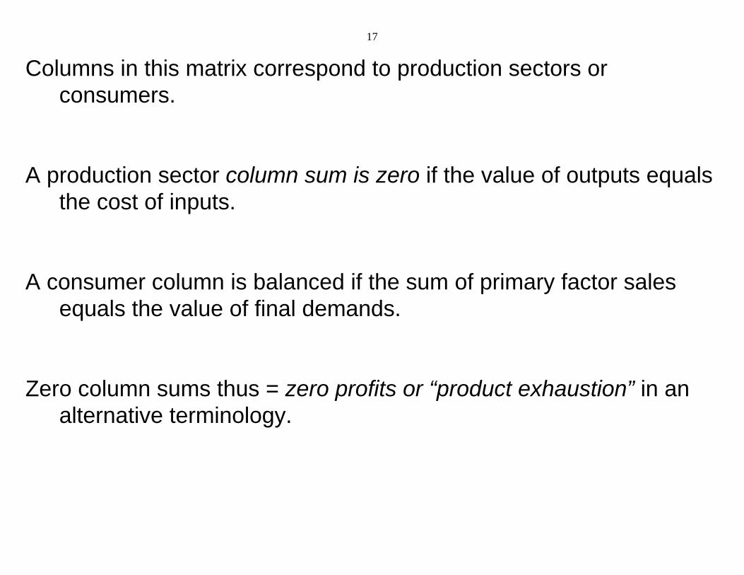
Columns in this matrix correspond to production sectors orconsumers.
A production sector column sum is zero if the value of outputs equalsthe cost of inputs.
A consumer column is balanced if the sum of primary factor salesequals the value of final demands.
Zero column sums thus = zero profits or “product exhaustion” in analternative terminology.
18
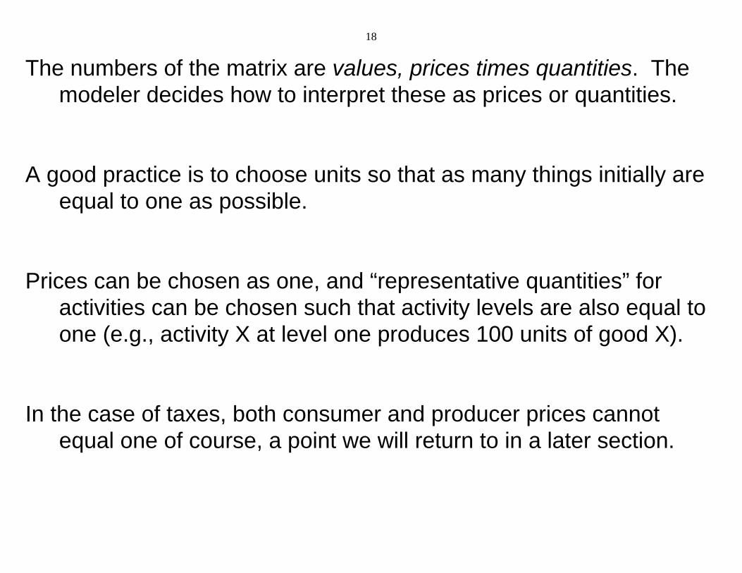
The numbers of the matrix are values, prices times quantities. Themodeler decides how to interpret these as prices or quantities.
A good practice is to choose units so that as many things initially areequal to one as possible.
Prices can be chosen as one, and “representative quantities” foractivities can be chosen such that activity levels are also equal toone (e.g., activity X at level one produces 100 units of good X).
In the case of taxes, both consumer and producer prices cannotequal one of course, a point we will return to in a later section.
19
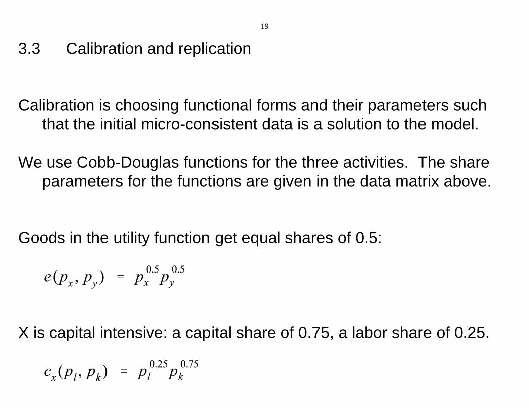
3.3 Calibration and replication
Calibration is choosing functional forms and their parameters suchthat the initial micro-consistent data is a solution to the model.
We use Cobb-Douglas functions for the three activities. The shareparameters for the functions are given in the data matrix above.
Goods in the utility function get equal shares of 0.5:
X is capital intensive: a capital share of 0.75, a labor share of 0.25.
20
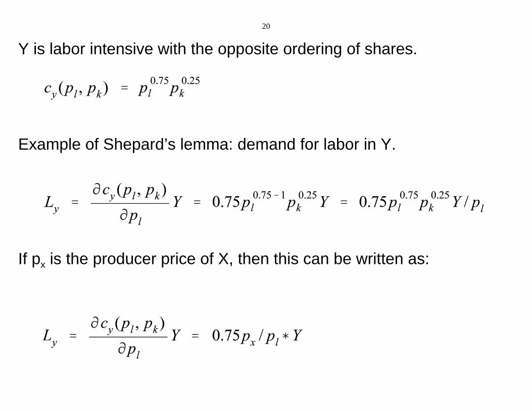
Y is labor intensive with the opposite ordering of shares.
Example of Shepard’s lemma: demand for labor in Y.
If px is the producer price of X, then this can be written as:
21
3.4 Model 3-4a
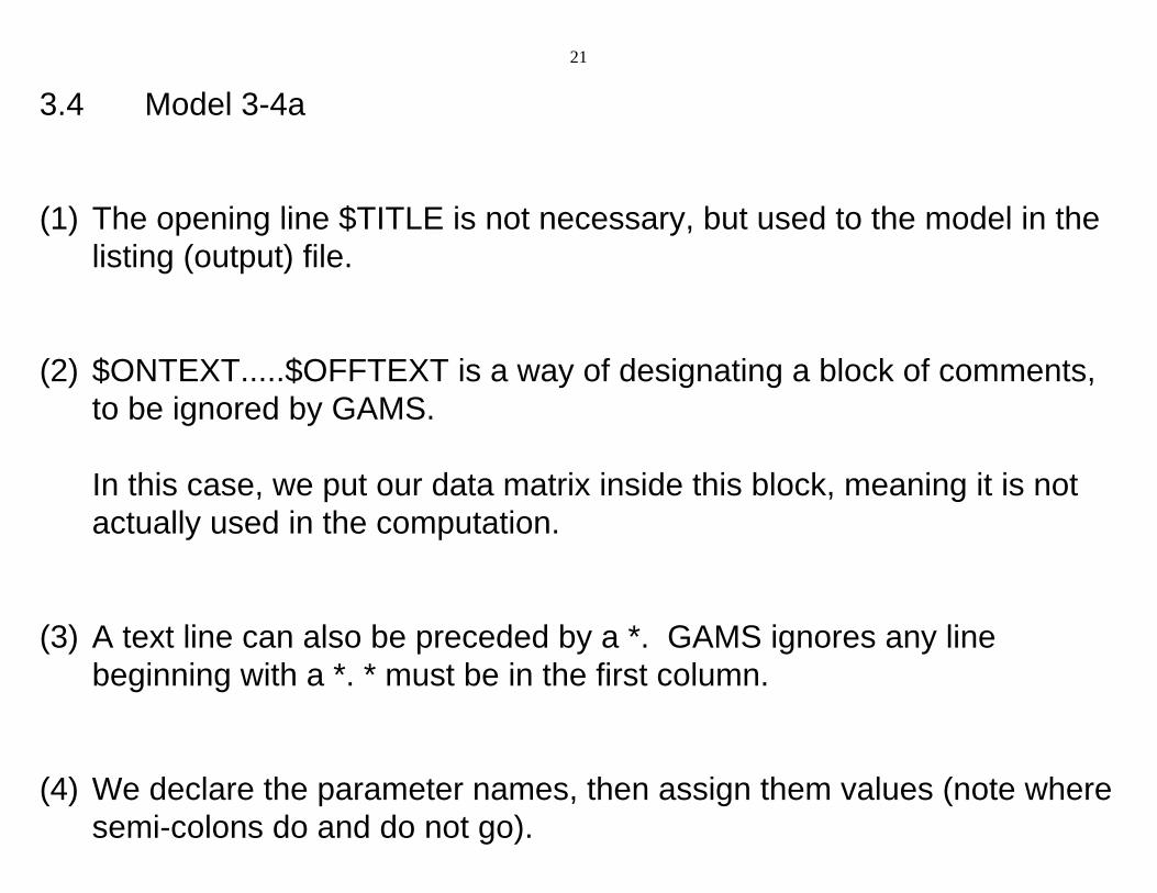
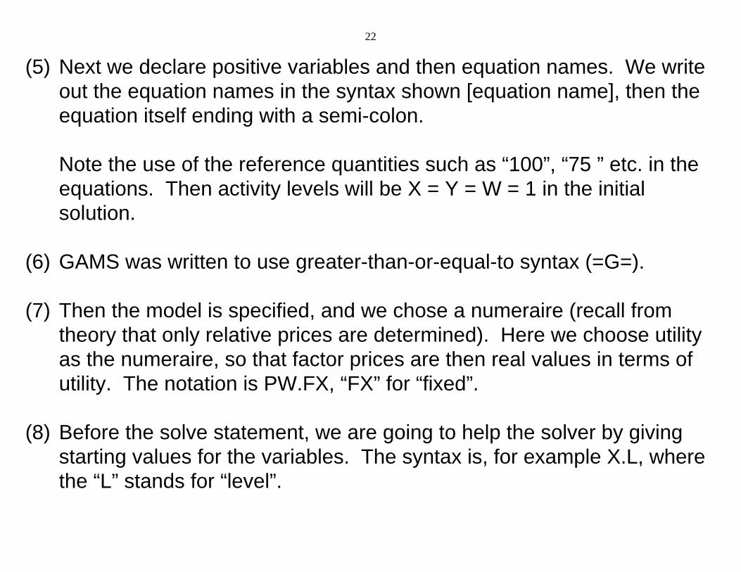
(1) The opening line $TITLE is not necessary, but used to the model in thelisting (output) file.
(2) $ONTEXT.....$OFFTEXT is a way of designating a block of comments,to be ignored by GAMS.
In this case, we put our data matrix inside this block, meaning it is notactually used in the computation.
(3) A text line can also be preceded by a *. GAMS ignores any linebeginning with a *. * must be in the first column.
(4) We declare the parameter names, then assign them values (note wheresemi-colons do and do not go).
22
(5) Next we declare positive variables and then equation names. We writeout the equation names in the syntax shown [equation name], then theequation itself ending with a semi-colon.
Note the use of the reference quantities such as “100”, “75 ” etc. in theequations. Then activity levels will be X = Y = W = 1 in the initialsolution.
(6) GAMS was written to use greater-than-or-equal-to syntax (=G=).
(7) Then the model is specified, and we chose a numeraire (recall fromtheory that only relative prices are determined). Here we choose utilityas the numeraire, so that factor prices are then real values in terms ofutility. The notation is PW.FX, “FX” for “fixed”.
(8) Before the solve statement, we are going to help the solver by givingstarting values for the variables. The syntax is, for example X.L, wherethe “L” stands for “level”.
23
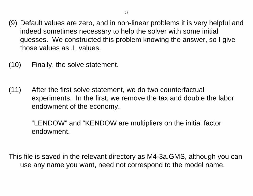
(9) Default values are zero, and in non-linear problems it is very helpful andindeed sometimes necessary to help the solver with some initialguesses. We constructed this problem knowing the answer, so I givethose values as .L values.
(10) Finally, the solve statement.
(11) After the first solve statement, we do two counterfactualexperiments. In the first, we remove the tax and double the laborendowment of the economy.
“LENDOW” and “KENDOW are multipliers on the initial factorendowment.
This file is saved in the relevant directory as M4-3a.GMS, although you canuse any name you want, need not correspond to the model name.
C:\jim\COURSES\8858\code-bk 2012\M3-4a.gms Monday, January 09, 2012 4:17:41 AM Page 1
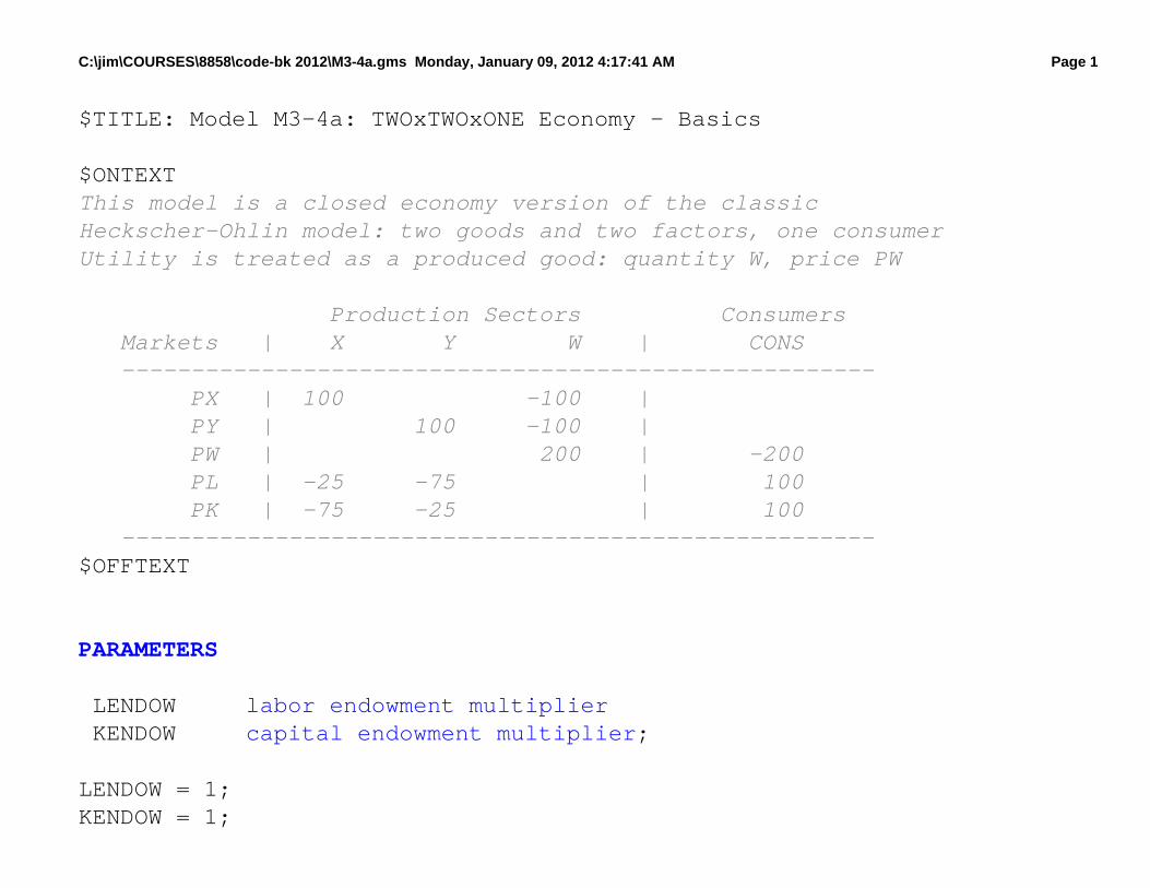
$TITLE: Model M3-4a: TWOxTWOxONE Economy - Basics
$ONTEXTThis model is a closed economy version of the classicHeckscher-Ohlin model: two goods and two factors, one consumerUtility is treated as a produced good: quantity W, price PW
Production Sectors Consumers Markets | X Y W | CONS ------------------------------------------------------ PX | 100 -100 | PY | 100 -100 | PW | 200 | -200 PL | -25 -75 | 100 PK | -75 -25 | 100 ------------------------------------------------------$OFFTEXT
PARAMETERS
L E N D O W labor endowment multiplier K E N D O W capital endowment multiplier;
LENDOW = 1;KENDOW = 1;
C:\jim\COURSES\8858\code-bk 2012\M3-4a.gms Monday, January 09, 2012 4:17:41 AM Page 2
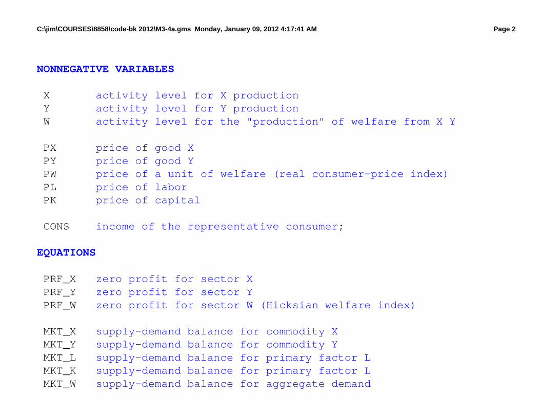
NONNEGATIVE VARIABLES
X activity level for X production Y activity level for Y production W activity level for the "production" of welfare from X Y
P X price of good X P Y price of good Y P W price of a unit of welfare (real consumer-price index) P L price of labor P K price of capital
C O N S income of the representative consumer;
EQUATIONS
P R F _ X zero profit for sector X P R F _ Y zero profit for sector Y P R F _ W zero profit for sector W (Hicksian welfare index)
M K T _ X supply-demand balance for commodity X M K T _ Y supply-demand balance for commodity Y M K T _ L supply-demand balance for primary factor L M K T _ K supply-demand balance for primary factor L M K T _ W supply-demand balance for aggregate demand
C:\jim\COURSES\8858\code-bk 2012\M3-4a.gms Monday, January 09, 2012 4:17:41 AM Page 3
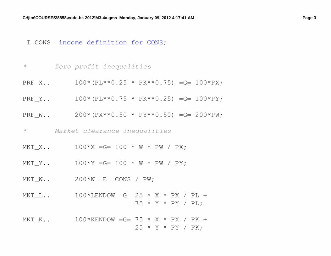
I _ C O N S income definition for CONS;
* Zero profit inequalities
PRF_X.. 100*(PL**0.25 * PK**0.75) =G= 100*PX;
PRF_Y.. 100*(PL**0.75 * PK**0.25) =G= 100*PY;
PRF_W.. 200*(PX**0.50 * PY**0.50) =G= 200*PW;
* Market clearance inequalities
MKT_X.. 100*X =G= 100 * W * PW / PX;
MKT_Y.. 100*Y =G= 100 * W * PW / PY;
MKT_W.. 200*W =E= CONS / PW;
MKT_L.. 100*LENDOW =G= 25 * X * PX / PL + 75 * Y * PY / PL;
MKT_K.. 100*KENDOW =G= 75 * X * PX / PK + 25 * Y * PY / PK;
C:\jim\COURSES\8858\code-bk 2012\M3-4a.gms Monday, January 09, 2012 4:17:41 AM Page 4
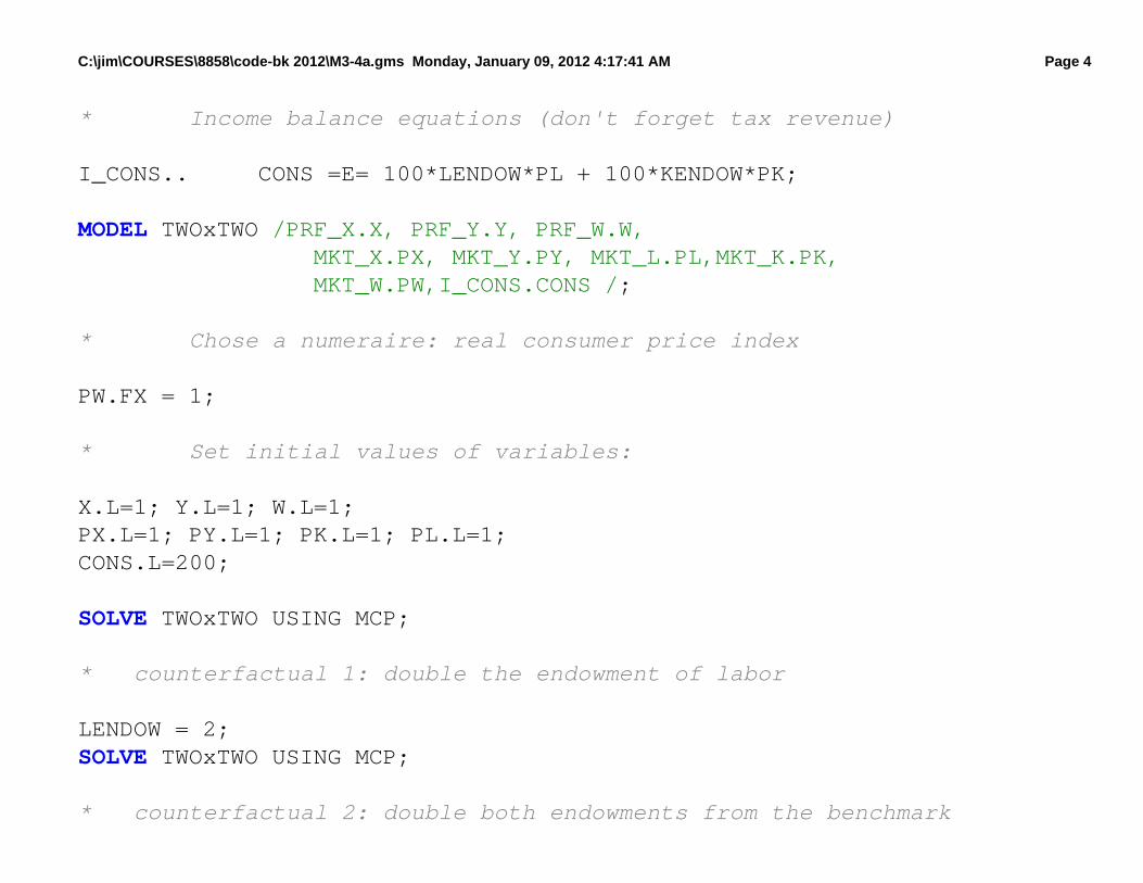
* Income balance equations (don't forget tax revenue)
I_CONS.. CONS =E= 100*LENDOW*PL + 100*KENDOW*PK;
MODEL TWOxTWO /PRF_X.X, PRF_Y.Y, PRF_W.W, MKT_X.PX, MKT_Y.PY, MKT_L.PL,MKT_K.PK, MKT_W.PW,I_CONS.CONS /;
* Chose a numeraire: real consumer price index
PW.FX = 1;
* Set initial values of variables:
X.L=1; Y.L=1; W.L=1;PX.L=1; PY.L=1; PK.L=1; PL.L=1;CONS.L=200;
SOLVE TWOxTWO USING MCP;
* counterfactual 1: double the endowment of labor
LENDOW = 2;SOLVE TWOxTWO USING MCP;
* counterfactual 2: double both endowments from the benchmark
C:\jim\COURSES\8858\code-bk 2012\M3-4a.gms Monday, January 09, 2012 4:17:41 AM Page 5
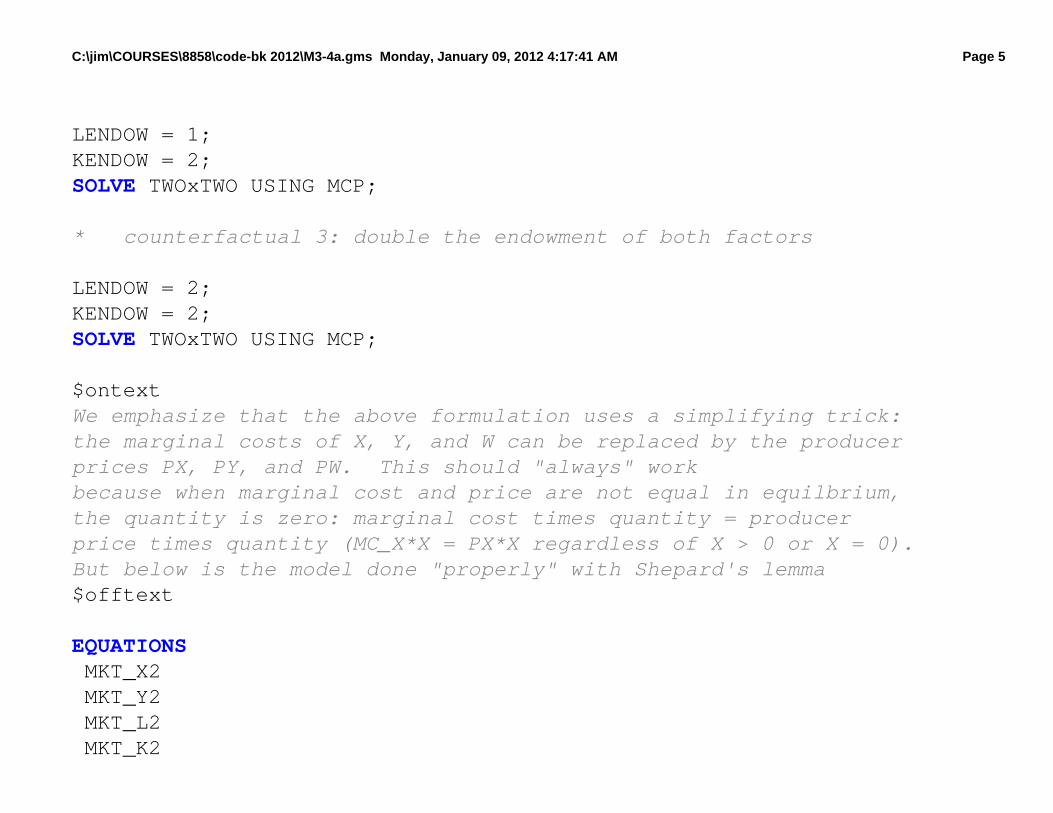
LENDOW = 1;KENDOW = 2;SOLVE TWOxTWO USING MCP;
* counterfactual 3: double the endowment of both factors
LENDOW = 2;KENDOW = 2;SOLVE TWOxTWO USING MCP;
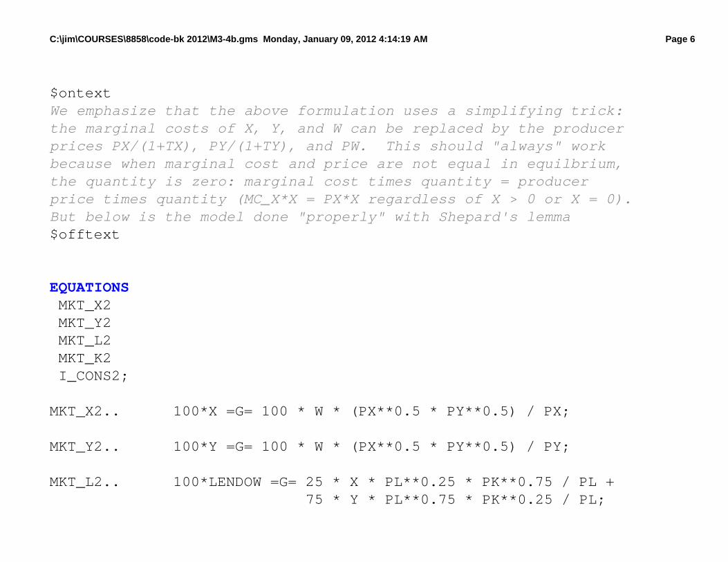
$ontextWe emphasize that the above formulation uses a simplifying trick:the marginal costs of X, Y, and W can be replaced by the producerprices PX, PY, and PW. This should "always" workbecause when marginal cost and price are not equal in equilbrium,the quantity is zero: marginal cost times quantity = producerprice times quantity (MC_X*X = PX*X regardless of X > 0 or X = 0).But below is the model done "properly" with Shepard's lemma$offtext
EQUATIONS MKT_X2 MKT_Y2 MKT_L2 MKT_K2
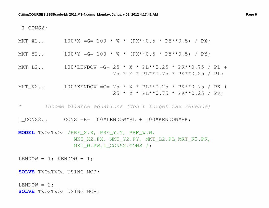
C:\jim\COURSES\8858\code-bk 2012\M3-4a.gms Monday, January 09, 2012 4:17:41 AM Page 6
I_CONS2;
MKT_X2.. 100*X =G= 100 * W * (PX**0.5 * PY**0.5) / PX;
MKT_Y2.. 100*Y =G= 100 * W * (PX**0.5 * PY**0.5) / PY;
MKT_L2.. 100*LENDOW =G= 25 * X * PL**0.25 * PK**0.75 / PL + 75 * Y * PL**0.75 * PK**0.25 / PL;
MKT_K2.. 100*KENDOW =G= 75 * X * PL**0.25 * PK**0.75 / PK + 25 * Y * PL**0.75 * PK**0.25 / PK;
* Income balance equations (don't forget tax revenue)
I_CONS2.. CONS =E= 100*LENDOW*PL + 100*KENDOW*PK;
MODEL TWOxTWOa /PRF_X.X, PRF_Y.Y, PRF_W.W, MKT_X2.PX, MKT_Y2.PY, MKT_L2.PL,MKT_K2.PK, MKT_W.PW,I_CONS2.CONS /;
LENDOW = 1; KENDOW = 1;
SOLVE TWOxTWOa USING MCP;
LENDOW = 2;SOLVE TWOxTWOa USING MCP;
C:\jim\COURSES\8858\code-bk 2012\M3-4a.gms Monday, January 09, 2012 4:17:41 AM Page 7
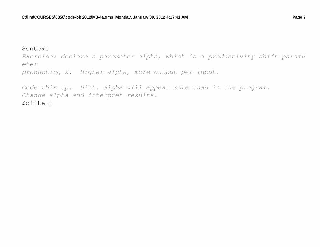
$ontextExercise: declare a parameter alpha, which is a productivity shift param»eterproducting X. Higher alpha, more output per input.
Code this up. Hint: alpha will appear more than in the program.Change alpha and interpret results.$offtext
24
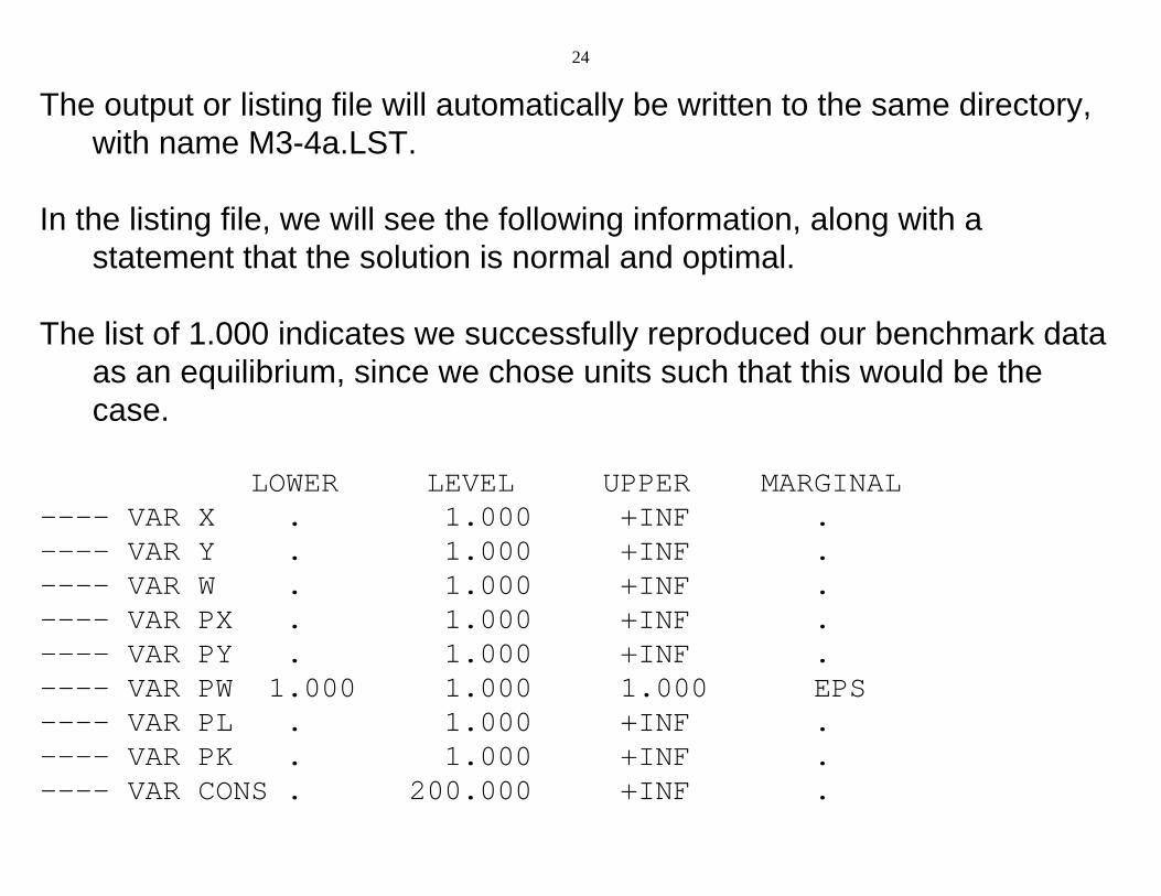
The output or listing file will automatically be written to the same directory,with name M3-4a.LST.
In the listing file, we will see the following information, along with astatement that the solution is normal and optimal.
The list of 1.000 indicates we successfully reproduced our benchmark dataas an equilibrium, since we chose units such that this would be thecase.
LOWER LEVEL UPPER MARGINAL ---- VAR X . 1.000 +INF . ---- VAR Y . 1.000 +INF . ---- VAR W . 1.000 +INF . ---- VAR PX . 1.000 +INF . ---- VAR PY . 1.000 +INF . ---- VAR PW 1.000 1.000 1.000 EPS ---- VAR PL . 1.000 +INF . ---- VAR PK . 1.000 +INF . ---- VAR CONS . 200.000 +INF .
25
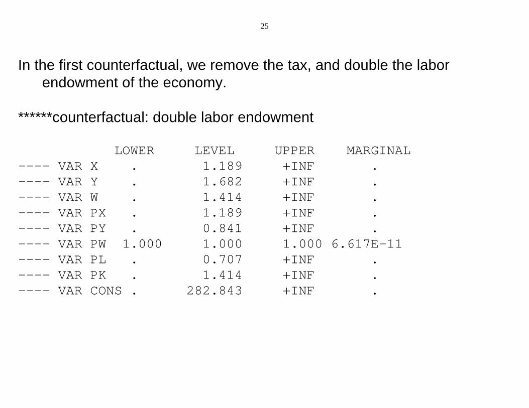
In the first counterfactual, we remove the tax, and double the laborendowment of the economy.
******counterfactual: double labor endowment
LOWER LEVEL UPPER MARGINAL ---- VAR X . 1.189 +INF . ---- VAR Y . 1.682 +INF . ---- VAR W . 1.414 +INF . ---- VAR PX . 1.189 +INF . ---- VAR PY . 0.841 +INF . ---- VAR PW 1.000 1.000 1.000 6.617E-11 ---- VAR PL . 0.707 +INF . ---- VAR PK . 1.414 +INF . ---- VAR CONS . 282.843 +INF .
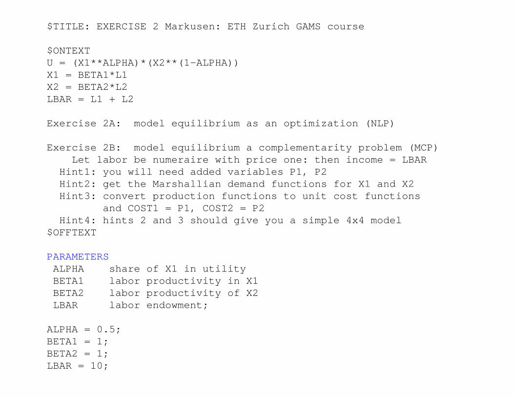
$TITLE: EXERCISE 2 Markusen: ETH Zurich GAMS course
$ONTEXTU = (X1**ALPHA)*(X2**(1-ALPHA))X1 = BETA1*L1X2 = BETA2*L2LBAR = L1 + L2
Exercise 2A: model equilibrium as an optimization (NLP)
Exercise 2B: model equilibrium a complementarity problem (MCP) Let labor be numeraire with price one: then income = LBAR Hint1: you will need added variables P1, P2 Hint2: get the Marshallian demand functions for X1 and X2 Hint3: convert production functions to unit cost functions and COST1 = P1, COST2 = P2 Hint4: hints 2 and 3 should give you a simple 4x4 model$OFFTEXT
PARAMETERS ALPHA share of X1 in utility BETA1 labor productivity in X1 BETA2 labor productivity of X2 LBAR labor endowment;
ALPHA = 0.5;BETA1 = 1;BETA2 = 1;LBAR = 10;
28
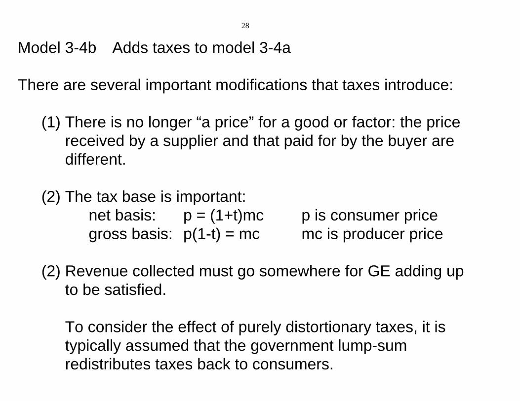
Model 3-4b Adds taxes to model 3-4a
There are several important modifications that taxes introduce:
(1) There is no longer “a price” for a good or factor: the pricereceived by a supplier and that paid for by the buyer aredifferent.
(2) The tax base is important:net basis: p = (1+t)mc p is consumer pricegross basis: p(1-t) = mc mc is producer price
(2) Revenue collected must go somewhere for GE adding upto be satisfied.
To consider the effect of purely distortionary taxes, it istypically assumed that the government lump-sumredistributes taxes back to consumers.
29
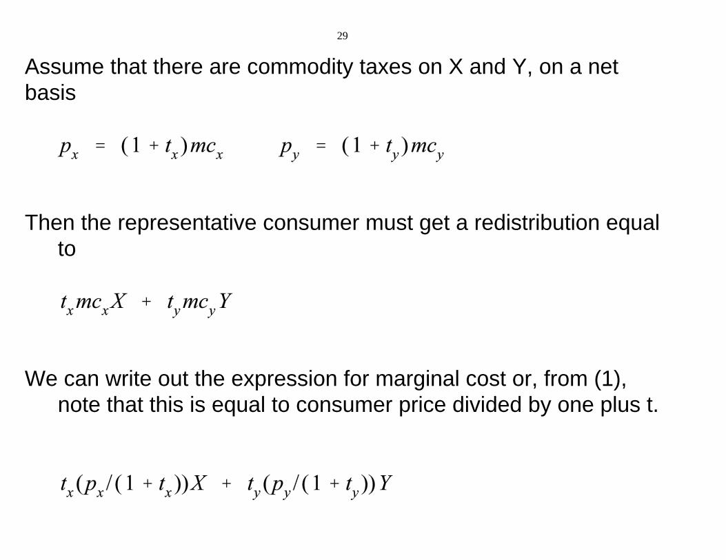
Assume that there are commodity taxes on X and Y, on a netbasis
Then the representative consumer must get a redistribution equalto
We can write out the expression for marginal cost or, from (1),note that this is equal to consumer price divided by one plus t.
C:\jim\COURSES\8858\code-bk 2012\M3-4b.gms Monday, January 09, 2012 4:14:19 AM Page 1
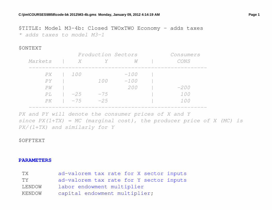
$TITLE: Model M3-4b: Closed TWOxTWO Economy - adds taxes* adds taxes to model M3-1
$ONTEXT Production Sectors Consumers Markets | X Y W | CONS ------------------------------------------------------ PX | 100 -100 | PY | 100 -100 | PW | 200 | -200 PL | -25 -75 | 100 PK | -75 -25 | 100 ------------------------------------------------------PX and PY will denote the consumer prices of X and Ysince PX(1+TX) = MC (marginal cost), the producer price of X (MC) isPX/(1+TX) and similarly for Y
$OFFTEXT
PARAMETERS
T X ad-valorem tax rate for X sector inputs T Y ad-valorem tax rate for Y sector inputs L E N D O W labor endowment multiplier K E N D O W capital endowment multiplier;
C:\jim\COURSES\8858\code-bk 2012\M3-4b.gms Monday, January 09, 2012 4:14:19 AM Page 2
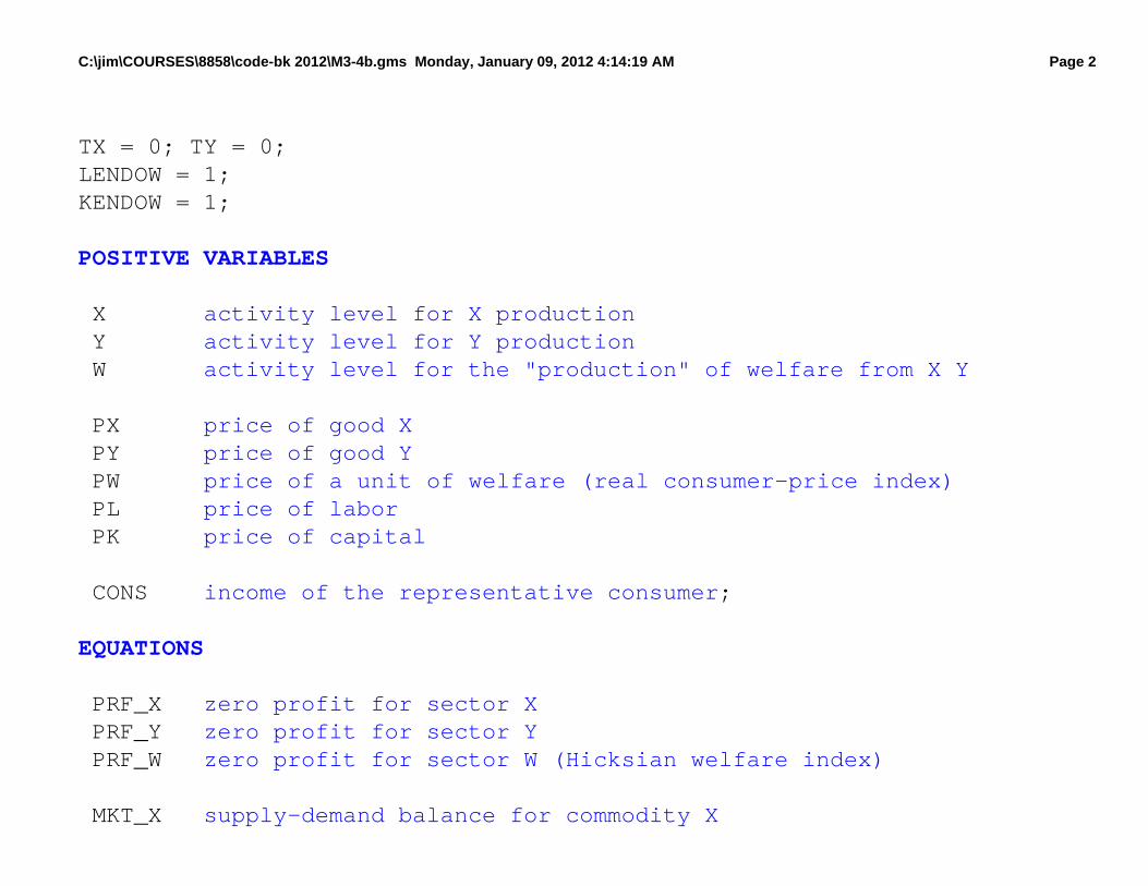
TX = 0; TY = 0;LENDOW = 1;KENDOW = 1;
POSITIVE VARIABLES
X activity level for X production Y activity level for Y production W activity level for the "production" of welfare from X Y
P X price of good X P Y price of good Y P W price of a unit of welfare (real consumer-price index) P L price of labor P K price of capital
C O N S income of the representative consumer;
EQUATIONS
P R F _ X zero profit for sector X P R F _ Y zero profit for sector Y P R F _ W zero profit for sector W (Hicksian welfare index)
M K T _ X supply-demand balance for commodity X
C:\jim\COURSES\8858\code-bk 2012\M3-4b.gms Monday, January 09, 2012 4:14:19 AM Page 3
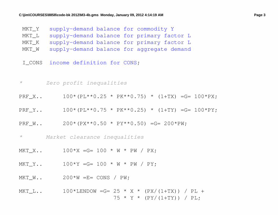
M K T _ Y supply-demand balance for commodity Y M K T _ L supply-demand balance for primary factor L M K T _ K supply-demand balance for primary factor L M K T _ W supply-demand balance for aggregate demand
I _ C O N S income definition for CONS;
* Zero profit inequalities
PRF_X.. 100*(PL**0.25 * PK**0.75) * (1+TX) =G= 100*PX;
PRF_Y.. 100*(PL**0.75 * PK**0.25) * (1+TY) =G= 100*PY;
PRF_W.. 200*(PX**0.50 * PY**0.50) =G= 200*PW;
* Market clearance inequalities
MKT_X.. 100*X =G= 100 * W * PW / PX;
MKT_Y.. 100*Y =G= 100 * W * PW / PY;
MKT_W.. 200*W =E= CONS / PW;
MKT_L.. 100*LENDOW =G= 25 * X * (PX/(1+TX)) / PL + 75 * Y * (PY/(1+TY)) / PL;
C:\jim\COURSES\8858\code-bk 2012\M3-4b.gms Monday, January 09, 2012 4:14:19 AM Page 4
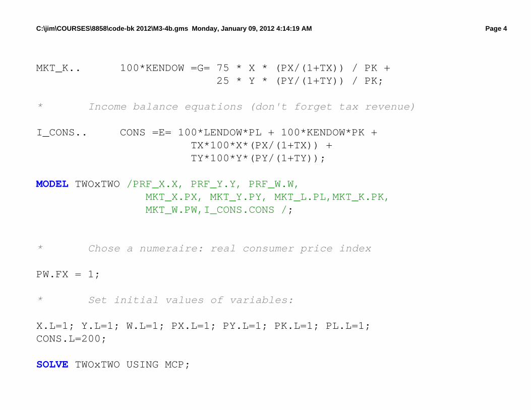
MKT_K.. 100*KENDOW =G= 75 * X * (PX/(1+TX)) / PK + 25 * Y * (PY/(1+TY)) / PK;
* Income balance equations (don't forget tax revenue)
I_CONS.. CONS =E= 100*LENDOW*PL + 100*KENDOW*PK + TX*100*X*(PX/(1+TX)) + TY*100*Y*(PY/(1+TY));
MODEL TWOxTWO /PRF_X.X, PRF_Y.Y, PRF_W.W, MKT_X.PX, MKT_Y.PY, MKT_L.PL,MKT_K.PK, MKT_W.PW,I_CONS.CONS /;
* Chose a numeraire: real consumer price index
PW.FX = 1;
* Set initial values of variables:
X.L=1; Y.L=1; W.L=1; PX.L=1; PY.L=1; PK.L=1; PL.L=1;CONS.L=200;
SOLVE TWOxTWO USING MCP;
C:\jim\COURSES\8858\code-bk 2012\M3-4b.gms Monday, January 09, 2012 4:14:19 AM Page 5
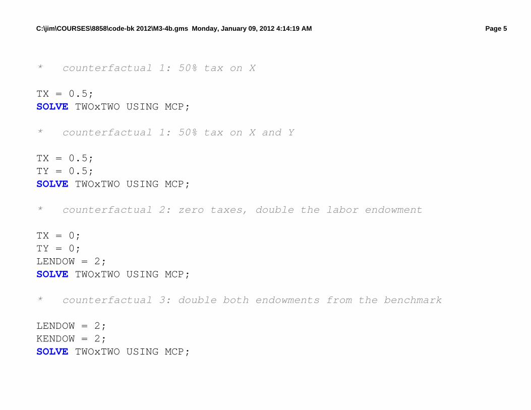
* counterfactual 1: 50% tax on X
TX = 0.5;SOLVE TWOxTWO USING MCP;
* counterfactual 1: 50% tax on X and Y
TX = 0.5;TY = 0.5;SOLVE TWOxTWO USING MCP;
* counterfactual 2: zero taxes, double the labor endowment
TX = 0;TY = 0;LENDOW = 2;SOLVE TWOxTWO USING MCP;
* counterfactual 3: double both endowments from the benchmark
LENDOW = 2;KENDOW = 2;SOLVE TWOxTWO USING MCP;
C:\jim\COURSES\8858\code-bk 2012\M3-4b.gms Monday, January 09, 2012 4:14:19 AM Page 6
$ontextWe emphasize that the above formulation uses a simplifying trick:the marginal costs of X, Y, and W can be replaced by the producerprices PX/(1+TX), PY/(1+TY), and PW. This should "always" workbecause when marginal cost and price are not equal in equilbrium,the quantity is zero: marginal cost times quantity = producerprice times quantity (MC_X*X = PX*X regardless of X > 0 or X = 0).But below is the model done "properly" with Shepard's lemma$offtext
EQUATIONS MKT_X2 MKT_Y2 MKT_L2 MKT_K2 I_CONS2;
MKT_X2.. 100*X =G= 100 * W * (PX**0.5 * PY**0.5) / PX;
MKT_Y2.. 100*Y =G= 100 * W * (PX**0.5 * PY**0.5) / PY;
MKT_L2.. 100*LENDOW =G= 25 * X * PL**0.25 * PK**0.75 / PL + 75 * Y * PL**0.75 * PK**0.25 / PL;
C:\jim\COURSES\8858\code-bk 2012\M3-4b.gms Monday, January 09, 2012 4:14:19 AM Page 7
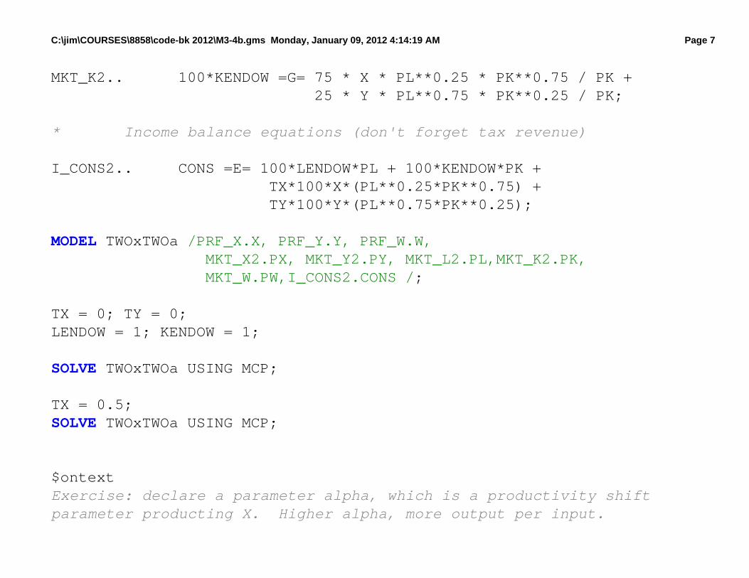
MKT_K2.. 100*KENDOW =G= 75 * X * PL**0.25 * PK**0.75 / PK + 25 * Y * PL**0.75 * PK**0.25 / PK;
* Income balance equations (don't forget tax revenue)
I_CONS2.. CONS =E= 100*LENDOW*PL + 100*KENDOW*PK + TX*100*X*(PL**0.25*PK**0.75) + TY*100*Y*(PL**0.75*PK**0.25);
MODEL TWOxTWOa /PRF_X.X, PRF_Y.Y, PRF_W.W, MKT_X2.PX, MKT_Y2.PY, MKT_L2.PL,MKT_K2.PK, MKT_W.PW,I_CONS2.CONS /;
TX = 0; TY = 0;LENDOW = 1; KENDOW = 1;
SOLVE TWOxTWOa USING MCP;
TX = 0.5;SOLVE TWOxTWOa USING MCP;
$ontextExercise: declare a parameter alpha, which is a productivity shiftparameter producting X. Higher alpha, more output per input.
C:\jim\COURSES\8858\code-bk 2012\M3-4b.gms Monday, January 09, 2012 4:14:19 AM Page 8
Code this up. Hint: alpha will appear more than in the program.Change alpha and interpret results.$offtext
30
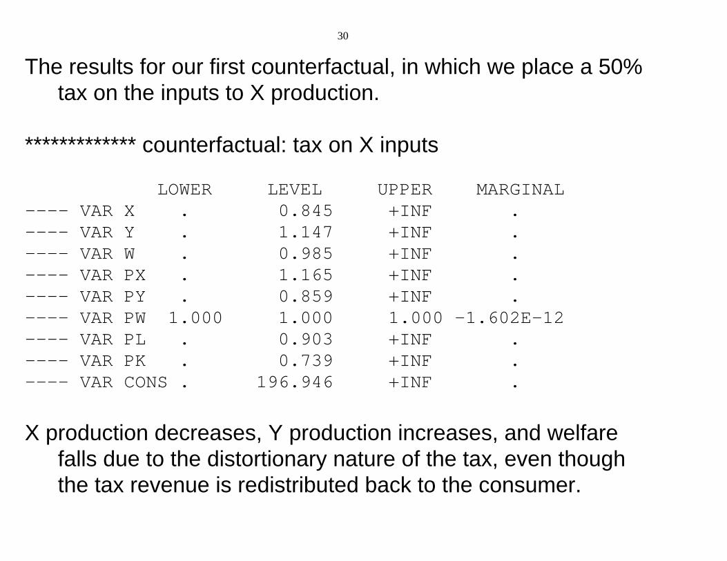
The results for our first counterfactual, in which we place a 50%tax on the inputs to X production.
************* counterfactual: tax on X inputs
LOWER LEVEL UPPER MARGINAL ---- VAR X . 0.845 +INF . ---- VAR Y . 1.147 +INF . ---- VAR W . 0.985 +INF . ---- VAR PX . 1.165 +INF . ---- VAR PY . 0.859 +INF . ---- VAR PW 1.000 1.000 1.000 -1.602E-12 ---- VAR PL . 0.903 +INF . ---- VAR PK . 0.739 +INF . ---- VAR CONS . 196.946 +INF .
X production decreases, Y production increases, and welfarefalls due to the distortionary nature of the tax, even thoughthe tax revenue is redistributed back to the consumer.
31
There is also a redistribution of income between factors.
The relative price of capital, the factor used intensively in X falls,and the relative price of labor rises as resources are shifted toY production.
32
3.5 Initially slack activities
As noted in chapter one, an attractive and powerful feature ofGAMS is that it solves complementarity problems in whichsome production activities can be slack for some values ofparameters and active for others.
This allows researchers to consider a much wider set ofproblems that is allowed using software which can only solvesystems of equations.
There are many uses of this in practice:alternative energy technologies that are unprofitable initiallyillegal activities that are inefficient relative to legal onestrade links that are initially inactive due to high trade costs
33
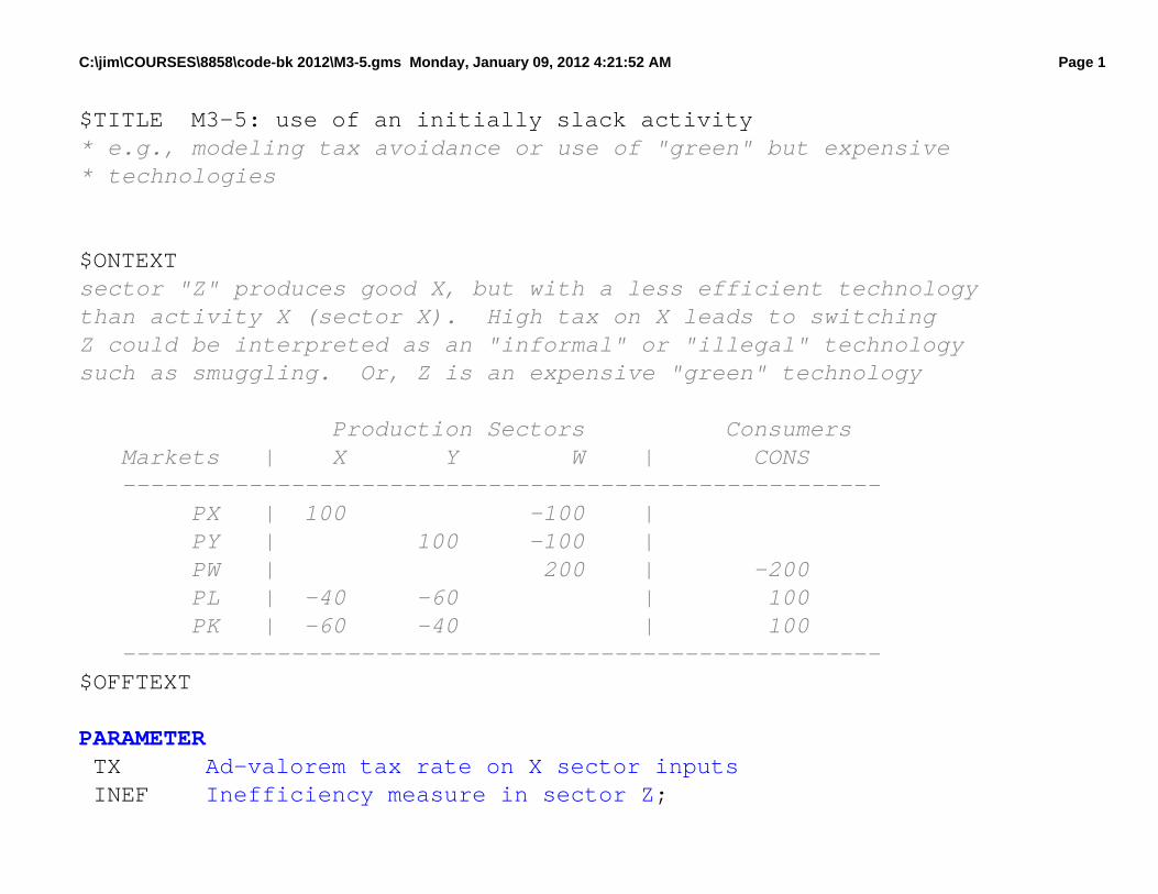
Model 3-5 presents an example, motivated by tax evasionactivities, or a “green” but expensive technology
A third sector, Z, also produces good X but it is 10% lessefficient (10% more costly) than the X activity itself. Soinitially, Z does not operate.
But when a tax of 25% is imposed on X, this activity goes slackand Z begins to operate.
We could think of Z as a tax evasion or “informal” activity that isless efficient but can successfully avoid the tax.
Another counterfactual assesses the effect of a 25% tax whenthe Z technology cannot operate, to assess switching costs.
34
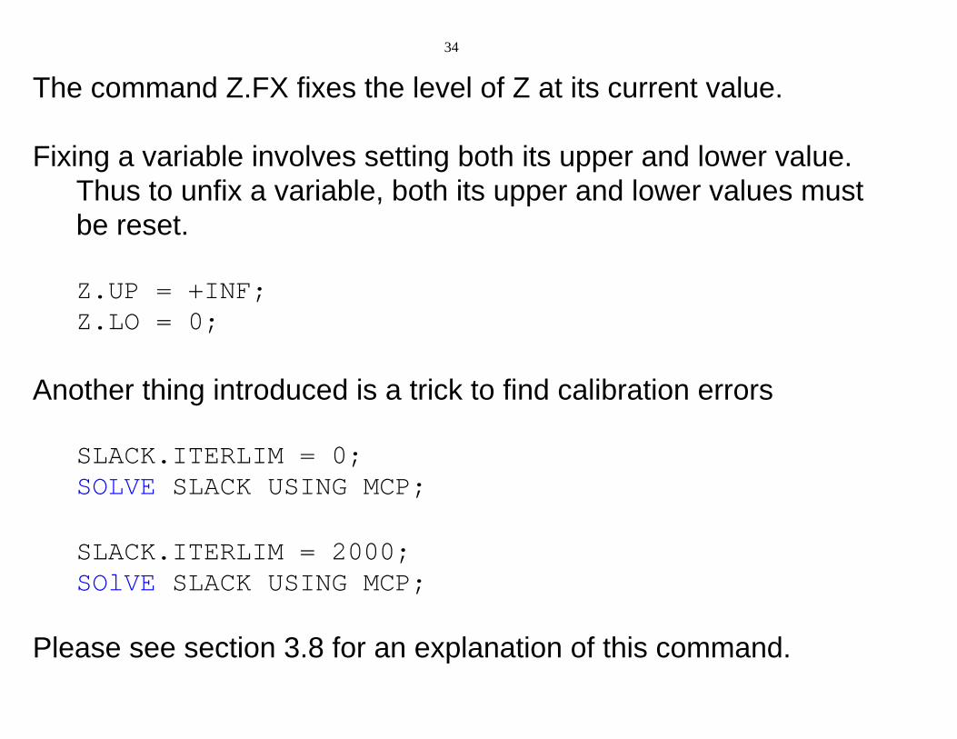
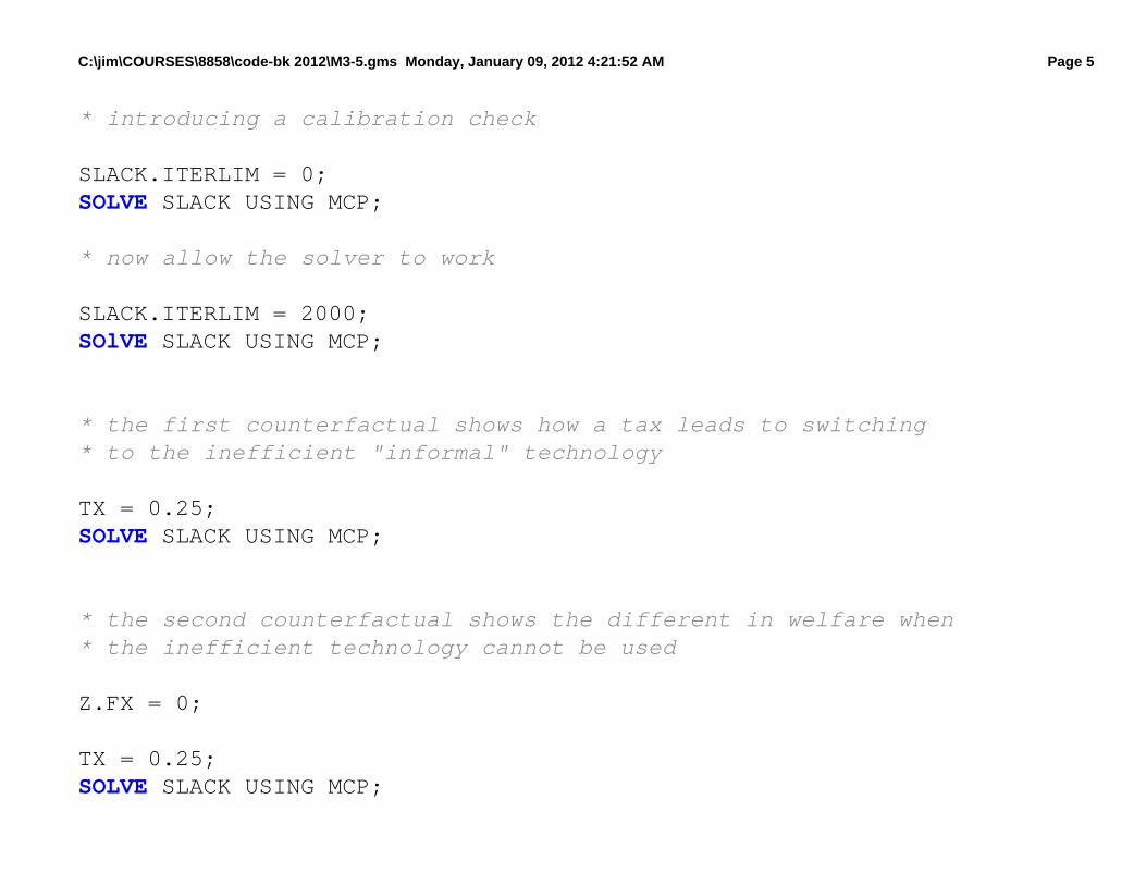
The command Z.FX fixes the level of Z at its current value.
Fixing a variable involves setting both its upper and lower value. Thus to unfix a variable, both its upper and lower values mustbe reset.
Z.UP = +INF;Z.LO = 0;
Another thing introduced is a trick to find calibration errors
SLACK.ITERLIM = 0;SOLVE SLACK USING MCP;
SLACK.ITERLIM = 2000;SOlVE SLACK USING MCP;
Please see section 3.8 for an explanation of this command.
C:\jim\COURSES\8858\code-bk 2012\M3-5.gms Monday, January 09, 2012 4:21:52 AM Page 1
$TITLE M3-5: use of an initially slack activity* e.g., modeling tax avoidance or use of "green" but expensive* technologies
$ONTEXTsector "Z" produces good X, but with a less efficient technologythan activity X (sector X). High tax on X leads to switchingZ could be interpreted as an "informal" or "illegal" technologysuch as smuggling. Or, Z is an expensive "green" technology
Production Sectors Consumers Markets | X Y W | CONS ------------------------------------------------------ PX | 100 -100 | PY | 100 -100 | PW | 200 | -200 PL | -40 -60 | 100 PK | -60 -40 | 100 ------------------------------------------------------$OFFTEXT
PARAMETER T X Ad-valorem tax rate on X sector inputs I N E F Inefficiency measure in sector Z;
C:\jim\COURSES\8858\code-bk 2012\M3-5.gms Monday, January 09, 2012 4:21:52 AM Page 2
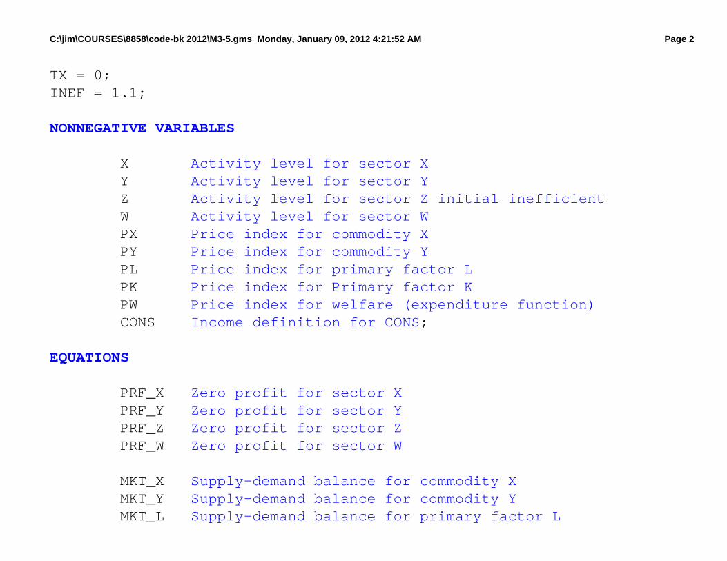
TX = 0;INEF = 1.1;
NONNEGATIVE VARIABLES
X Activity level for sector X Y Activity level for sector Y Z Activity level for sector Z initial inefficient W Activity level for sector W P X Price index for commodity X P Y Price index for commodity Y P L Price index for primary factor L P K Price index for Primary factor K P W Price index for welfare (expenditure function) C O N S Income definition for CONS;
EQUATIONS
P R F _ X Zero profit for sector X P R F _ Y Zero profit for sector Y P R F _ Z Zero profit for sector Z P R F _ W Zero profit for sector W
M K T _ X Supply-demand balance for commodity X M K T _ Y Supply-demand balance for commodity Y M K T _ L Supply-demand balance for primary factor L
C:\jim\COURSES\8858\code-bk 2012\M3-5.gms Monday, January 09, 2012 4:21:52 AM Page 3
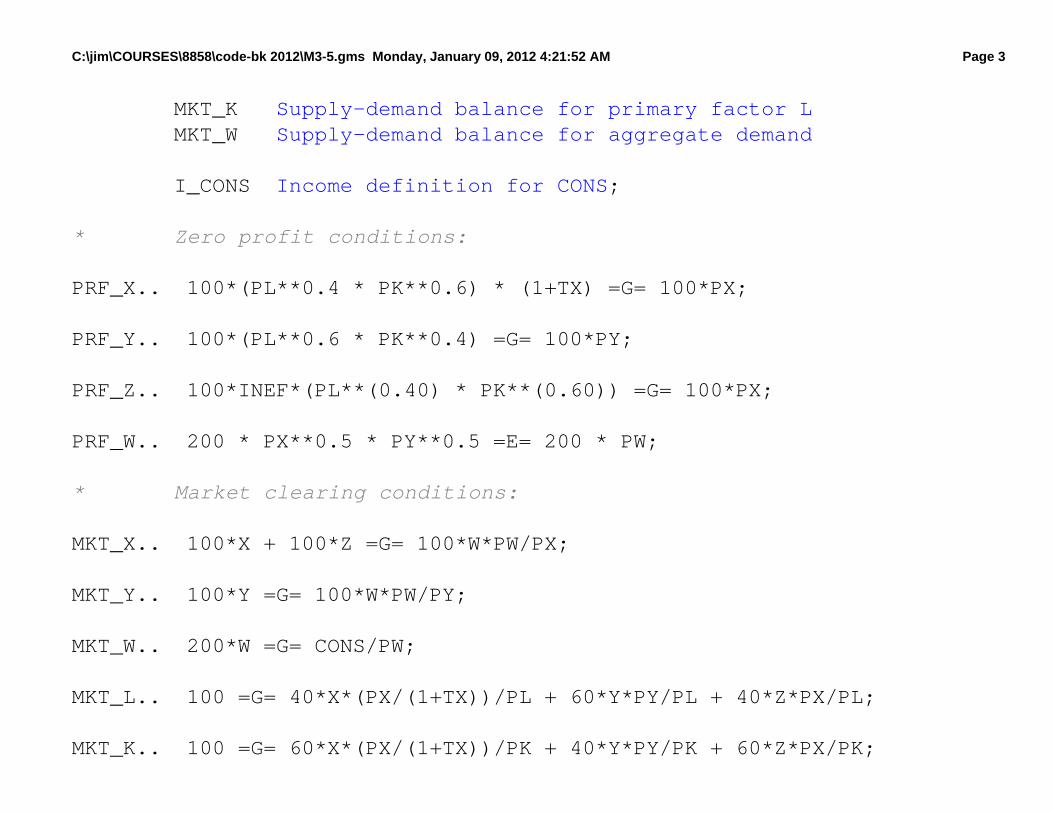
M K T _ K Supply-demand balance for primary factor L M K T _ W Supply-demand balance for aggregate demand
I _ C O N S Income definition for CONS;
* Zero profit conditions:
PRF_X.. 100*(PL**0.4 * PK**0.6) * (1+TX) =G= 100*PX;
PRF_Y.. 100*(PL**0.6 * PK**0.4) =G= 100*PY;
PRF_Z.. 100*INEF*(PL**(0.40) * PK**(0.60)) =G= 100*PX;
PRF_W.. 200 * PX**0.5 * PY**0.5 =E= 200 * PW;
* Market clearing conditions:
MKT_X.. 100*X + 100*Z =G= 100*W*PW/PX;
MKT_Y.. 100*Y =G= 100*W*PW/PY;
MKT_W.. 200*W =G= CONS/PW;
MKT_L.. 100 =G= 40*X*(PX/(1+TX))/PL + 60*Y*PY/PL + 40*Z*PX/PL;
MKT_K.. 100 =G= 60*X*(PX/(1+TX))/PK + 40*Y*PY/PK + 60*Z*PX/PK;
C:\jim\COURSES\8858\code-bk 2012\M3-5.gms Monday, January 09, 2012 4:21:52 AM Page 4
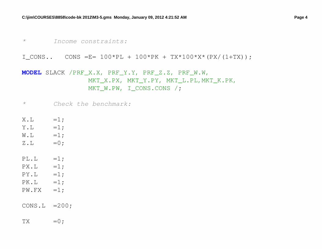
* Income constraints:
I_CONS.. CONS =E= 100*PL + 100*PK + TX*100*X*(PX/(1+TX));
MODEL SLACK /PRF_X.X, PRF_Y.Y, PRF_Z.Z, PRF_W.W, MKT_X.PX, MKT_Y.PY, MKT_L.PL,MKT_K.PK, MKT_W.PW, I_CONS.CONS /;
* Check the benchmark:
X.L =1;Y.L =1;W.L =1;Z.L =0;
PL.L =1;PX.L =1;PY.L =1;PK.L =1;PW.FX =1;
CONS.L =200;
TX =0;
C:\jim\COURSES\8858\code-bk 2012\M3-5.gms Monday, January 09, 2012 4:21:52 AM Page 5
* introducing a calibration check
SLACK.ITERLIM = 0;SOLVE SLACK USING MCP;
* now allow the solver to work
SLACK.ITERLIM = 2000;SOlVE SLACK USING MCP;
* the first counterfactual shows how a tax leads to switching* to the inefficient "informal" technology
TX = 0.25;SOLVE SLACK USING MCP;
* the second counterfactual shows the different in welfare when* the inefficient technology cannot be used
Z.FX = 0;
TX = 0.25;SOLVE SLACK USING MCP;
C:\jim\COURSES\8858\code-bk 2012\M3-5.gms Monday, January 09, 2012 4:21:52 AM Page 6
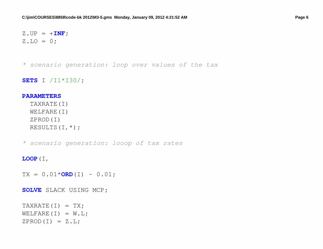
Z.UP = +INF;Z.LO = 0;
* scenario generation: loop over values of the tax
SETS I /I1*I30/;
PARAMETERS TAXRATE(I) WELFARE(I) ZPROD(I) RESULTS(I,*);
* scenario generation: looop of tax rates
LOOP(I,
TX = 0.01*ORD(I) - 0.01;
SOLVE SLACK USING MCP;
TAXRATE(I) = TX;WELFARE(I) = W.L;ZPROD(I) = Z.L;
C:\jim\COURSES\8858\code-bk 2012\M3-5.gms Monday, January 09, 2012 4:21:52 AM Page 7
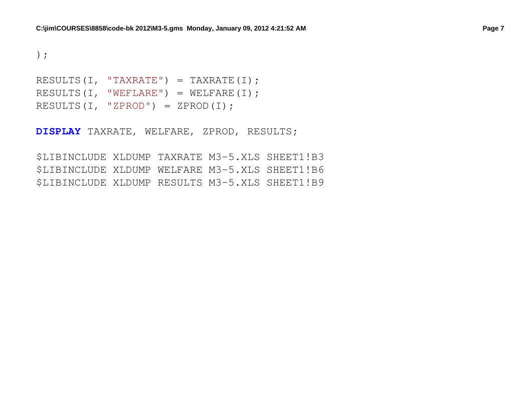
);
RESULTS(I, "TAXRATE") = TAXRATE(I);RESULTS(I, "WEFLARE") = WELFARE(I);RESULTS(I, "ZPROD") = ZPROD(I);
DISPLAY TAXRATE, WELFARE, ZPROD, RESULTS;
$LIBINCLUDE XLDUMP TAXRATE M3-5.XLS SHEET1!B3$LIBINCLUDE XLDUMP WELFARE M3-5.XLS SHEET1!B6$LIBINCLUDE XLDUMP RESULTS M3-5.XLS SHEET1!B9
35
3.6 Labor/leisure decision
Often general-equilibrium models used in international tradeassume that factors of production, especially labor, are infixed and inelastic supply.
But designing tax, welfare, and education systems, endogenizinglabor supply is a crucial part of the story.
Model M3-6 endogenizes labor supply, allowing labor to chosebetween leisure and labor supply with leisure entering into theworkers utility function.
In our formulation, we introduce an additional activity T, whichtransforms leisure (price PL) into labor supplied (price PLS).
36
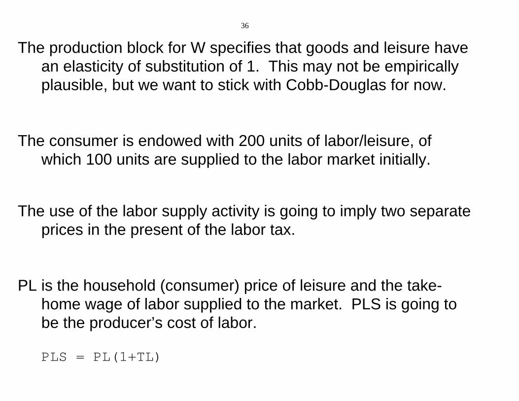
The production block for W specifies that goods and leisure havean elasticity of substitution of 1. This may not be empiricallyplausible, but we want to stick with Cobb-Douglas for now.
The consumer is endowed with 200 units of labor/leisure, ofwhich 100 units are supplied to the labor market initially.
The use of the labor supply activity is going to imply two separateprices in the present of the labor tax.
PL is the household (consumer) price of leisure and the take-home wage of labor supplied to the market. PLS is going tobe the producer’s cost of labor.
PLS = PL(1+TL)
37
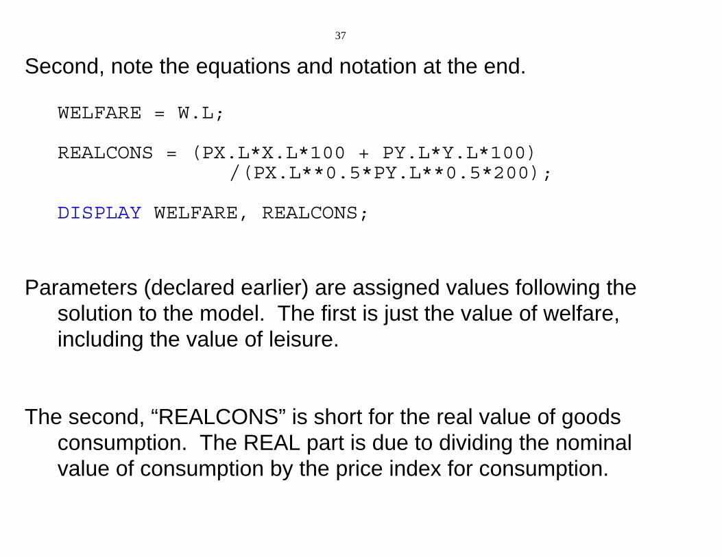
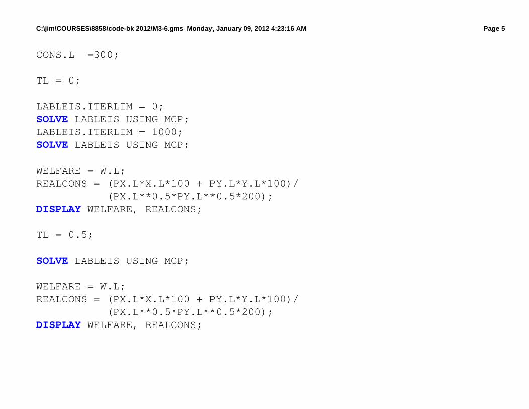
Second, note the equations and notation at the end.
WELFARE = W.L;
REALCONS = (PX.L*X.L*100 + PY.L*Y.L*100) /(PX.L**0.5*PY.L**0.5*200);
DISPLAY WELFARE, REALCONS;
Parameters (declared earlier) are assigned values following thesolution to the model. The first is just the value of welfare,including the value of leisure.
The second, “REALCONS” is short for the real value of goodsconsumption. The REAL part is due to dividing the nominalvalue of consumption by the price index for consumption.
38
As you will see if you run this model, the labor tax leads to areduction in labor supply.
This of course leads to a fall in commodity consumption but alsoto a rise in leisure.
Thus in this case, the usual statistics overstate the burden of thetax and would overstate the benefit of removing the tax iflabor supply increases (leisure falls).
C:\jim\COURSES\8858\code-bk 2012\M3-6.gms Monday, January 09, 2012 4:23:16 AM Page 1
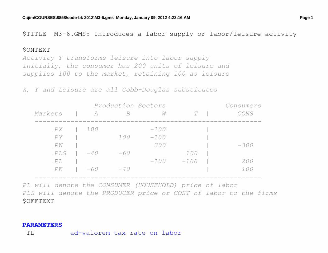
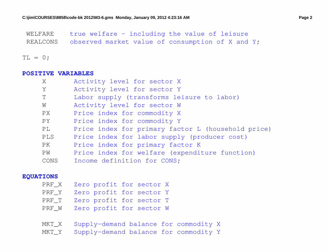
$TITLE M3-6.GMS: Introduces a labor supply or labor/leisure activity
$ONTEXTActivity T transforms leisure into labor supplyInitially, the consumer has 200 units of leisure andsupplies 100 to the market, retaining 100 as leisure
X, Y and Leisure are all Cobb-Douglas substitutes
Production Sectors Consumers Markets | A B W T | CONS --------------------------------------------------------- PX | 100 -100 | PY | 100 -100 | PW | 300 | -300 PLS | -40 -60 100 | PL | -100 -100 | 200 PK | -60 -40 | 100 ---------------------------------------------------------PL will denote the CONSUMER (HOUSEHOLD) price of laborPLS will denote the PRODUCER price or COST of labor to the firms$OFFTEXT
PARAMETERS T L ad-valorem tax rate on labor
C:\jim\COURSES\8858\code-bk 2012\M3-6.gms Monday, January 09, 2012 4:23:16 AM Page 2
W E L F A R E true welfare - including the value of leisure R E A L C O N S observed market value of consumption of X and Y;
TL = 0;
POSITIVE VARIABLES X Activity level for sector X Y Activity level for sector Y T Labor supply (transforms leisure to labor) W Activity level for sector W P X Price index for commodity X P Y Price index for commodity Y P L Price index for primary factor L (household price) P L S Price index for labor supply (producer cost) P K Price index for primary factor K P W Price index for welfare (expenditure function) C O N S Income definition for CONS;
EQUATIONS P R F _ X Zero profit for sector X P R F _ Y Zero profit for sector Y P R F _ T Zero profit for sector T P R F _ W Zero profit for sector W
M K T _ X Supply-demand balance for commodity X M K T _ Y Supply-demand balance for commodity Y
C:\jim\COURSES\8858\code-bk 2012\M3-6.gms Monday, January 09, 2012 4:23:16 AM Page 3
M K T _ L Supply-demand balance for primary factor L M K T _ L S Supply-demand balance for Leisure M K T _ K Supply-demand balance for primary factor K M K T _ W Supply-demand balance for aggregate demand
I _ C O N S Income definition for CONS;
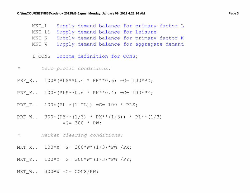
* Zero profit conditions:
PRF_X.. 100*(PLS**0.4 * PK**0.6) =G= 100*PX;
PRF_Y.. 100*(PLS**0.6 * PK**0.4) =G= 100*PY;
PRF_T.. 100*(PL *(1+TL)) =G= 100 * PLS;
PRF_W.. 300*(PY**(1/3) * PX**(1/3)) * PL**(1/3) =G= 300 * PW;
* Market clearing conditions:
MKT_X.. 100*X =G= 300*W*(1/3)*PW /PX;
MKT_Y.. 100*Y =G= 300*W*(1/3)*PW /PY;
MKT_W.. 300*W =G= CONS/PW;
C:\jim\COURSES\8858\code-bk 2012\M3-6.gms Monday, January 09, 2012 4:23:16 AM Page 4
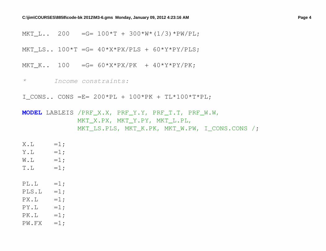
MKT_L.. 200 =G= 100*T + 300*W*(1/3)*PW/PL;
MKT_LS.. 100*T =G= 40*X*PX/PLS + 60*Y*PY/PLS;
MKT_K.. 100 =G= 60*X*PX/PK + 40*Y*PY/PK;
* Income constraints:
I_CONS.. CONS =E= 200*PL + 100*PK + TL*100*T*PL;
MODEL LABLEIS /PRF_X.X, PRF_Y.Y, PRF_T.T, PRF_W.W, MKT_X.PX, MKT_Y.PY, MKT_L.PL, MKT_LS.PLS, MKT_K.PK, MKT_W.PW, I_CONS.CONS /;
X.L =1;Y.L =1;W.L =1;T.L =1;
PL.L =1;PLS.L =1;PX.L =1;PY.L =1;PK.L =1;PW.FX =1;
C:\jim\COURSES\8858\code-bk 2012\M3-6.gms Monday, January 09, 2012 4:23:16 AM Page 5
CONS.L =300;
TL = 0;
LABLEIS.ITERLIM = 0;SOLVE LABLEIS USING MCP;LABLEIS.ITERLIM = 1000;SOLVE LABLEIS USING MCP;
WELFARE = W.L;REALCONS = (PX.L*X.L*100 + PY.L*Y.L*100)/ (PX.L**0.5*PY.L**0.5*200);DISPLAY WELFARE, REALCONS;
TL = 0.5;
SOLVE LABLEIS USING MCP;
WELFARE = W.L;REALCONS = (PX.L*X.L*100 + PY.L*Y.L*100)/ (PX.L**0.5*PY.L**0.5*200);DISPLAY WELFARE, REALCONS;
39
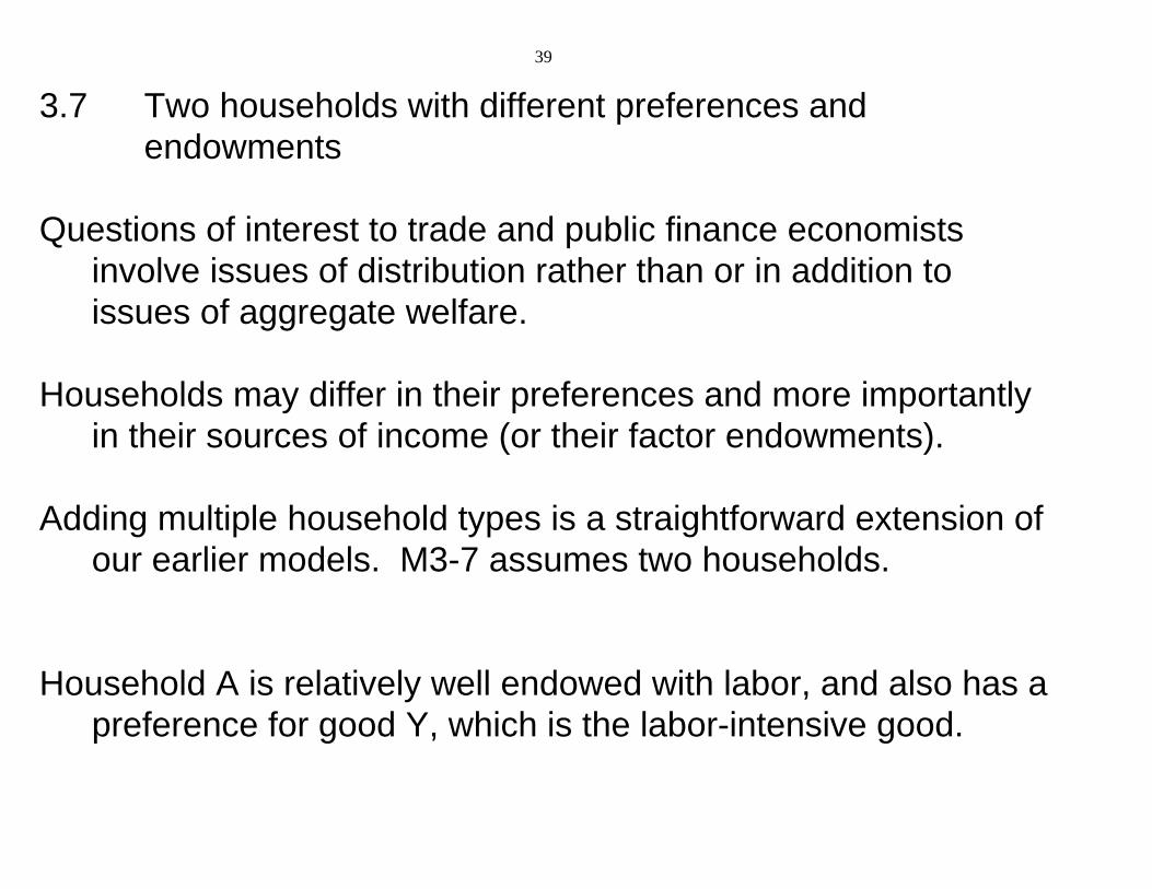
3.7 Two households with different preferences andendowments
Questions of interest to trade and public finance economistsinvolve issues of distribution rather than or in addition toissues of aggregate welfare.
Households may differ in their preferences and more importantlyin their sources of income (or their factor endowments).
Adding multiple household types is a straightforward extension ofour earlier models. M3-7 assumes two households.
Household A is relatively well endowed with labor, and also has apreference for good Y, which is the labor-intensive good.
40
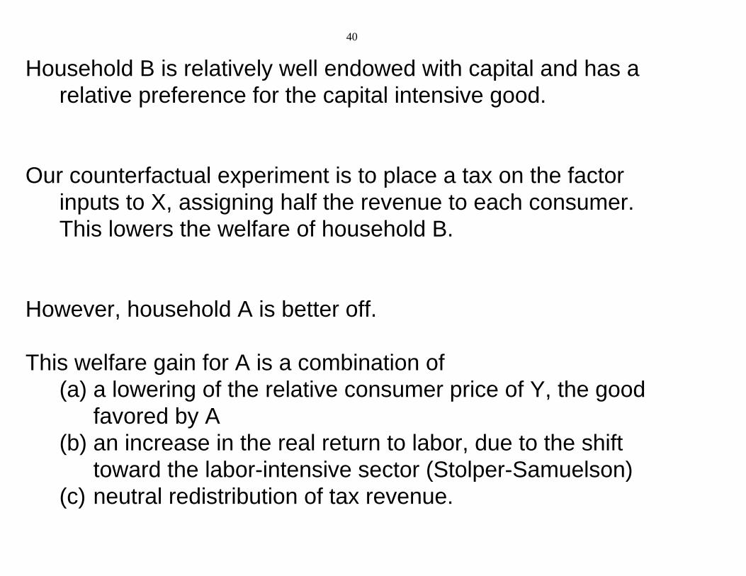
Household B is relatively well endowed with capital and has arelative preference for the capital intensive good.
Our counterfactual experiment is to place a tax on the factorinputs to X, assigning half the revenue to each consumer. This lowers the welfare of household B.
However, household A is better off.
This welfare gain for A is a combination of(a) a lowering of the relative consumer price of Y, the good
favored by A(b) an increase in the real return to labor, due to the shift
toward the labor-intensive sector (Stolper-Samuelson)(c) neutral redistribution of tax revenue.
C:\jim\COURSES\8858\code 2012\M3-7.gms Monday, January 30, 2012 2:12:56 PM Page 1
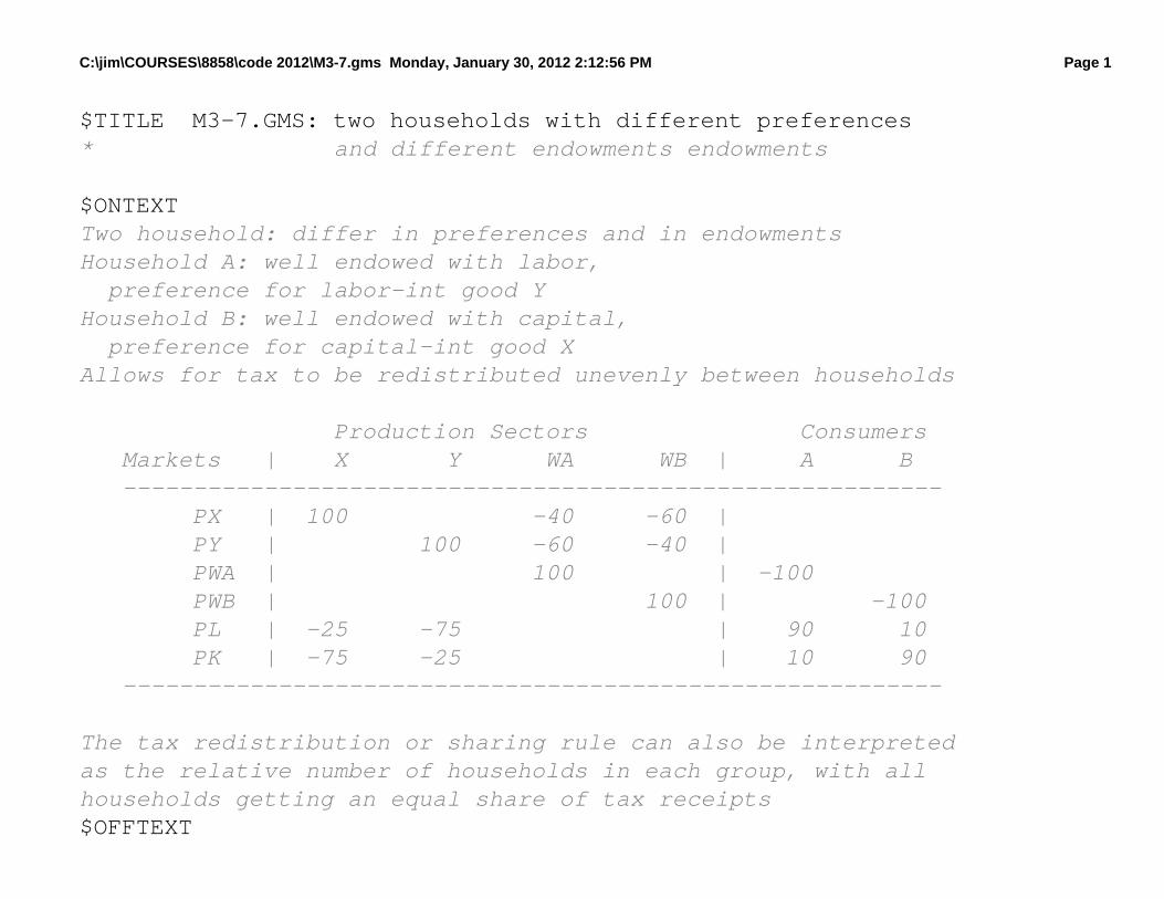
$TITLE M3-7.GMS: two households with different preferences* and different endowments endowments
$ONTEXTTwo household: differ in preferences and in endowmentsHousehold A: well endowed with labor, preference for labor-int good YHousehold B: well endowed with capital, preference for capital-int good XAllows for tax to be redistributed unevenly between households
Production Sectors Consumers Markets | X Y WA WB | A B ---------------------------------------------------------- PX | 100 -40 -60 | PY | 100 -60 -40 | PWA | 100 | -100 PWB | 100 | -100 PL | -25 -75 | 90 10 PK | -75 -25 | 10 90 ----------------------------------------------------------
The tax redistribution or sharing rule can also be interpretedas the relative number of households in each group, with allhouseholds getting an equal share of tax receipts$OFFTEXT
C:\jim\COURSES\8858\code 2012\M3-7.gms Monday, January 30, 2012 2:12:56 PM Page 2
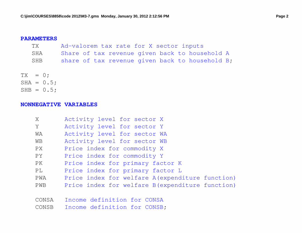
PARAMETERS T X Ad-valorem tax rate for X sector inputs S H A Share of tax revenue given back to household A S H B share of tax revenue given back to household B;
TX = 0;SHA = 0.5;SHB = 0.5;
NONNEGATIVE VARIABLES
X Activity level for sector X Y Activity level for sector Y W A Activity level for sector WA W B Activity level for sector WB P X Price index for commodity X P Y Price index for commodity Y P K Price index for primary factor K P L Price index for primary factor L P W A Price index for welfare A(expenditure function) P W B Price index for welfare B(expenditure function)
C O N S A Income definition for CONSA C O N S B Income definition for CONSB;
C:\jim\COURSES\8858\code 2012\M3-7.gms Monday, January 30, 2012 2:12:56 PM Page 3
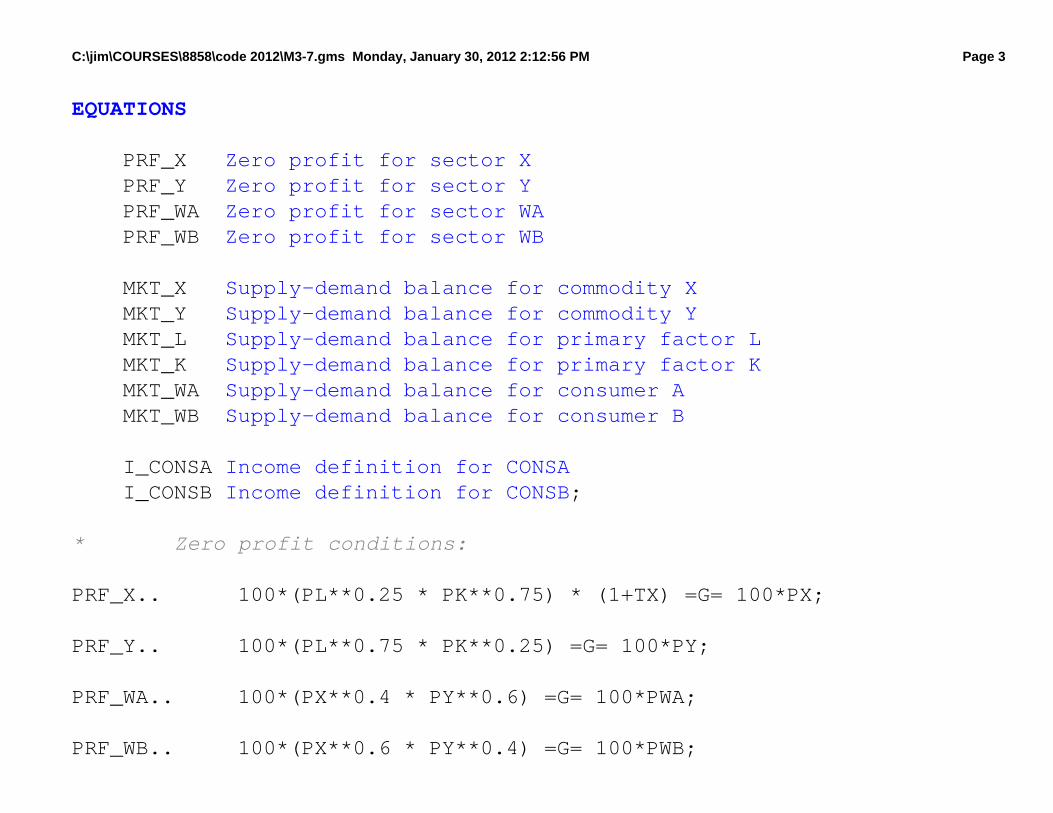
EQUATIONS
P R F _ X Zero profit for sector X P R F _ Y Zero profit for sector Y P R F _ W A Zero profit for sector WA P R F _ W B Zero profit for sector WB
M K T _ X Supply-demand balance for commodity X M K T _ Y Supply-demand balance for commodity Y M K T _ L Supply-demand balance for primary factor L M K T _ K Supply-demand balance for primary factor K M K T _ W A Supply-demand balance for consumer A M K T _ W B Supply-demand balance for consumer B
I _ C O N S A Income definition for CONSA I _ C O N S B Income definition for CONSB;
* Zero profit conditions:
PRF_X.. 100*(PL**0.25 * PK**0.75) * (1+TX) =G= 100*PX;
PRF_Y.. 100*(PL**0.75 * PK**0.25) =G= 100*PY;
PRF_WA.. 100*(PX**0.4 * PY**0.6) =G= 100*PWA;
PRF_WB.. 100*(PX**0.6 * PY**0.4) =G= 100*PWB;
C:\jim\COURSES\8858\code 2012\M3-7.gms Monday, January 30, 2012 2:12:56 PM Page 4
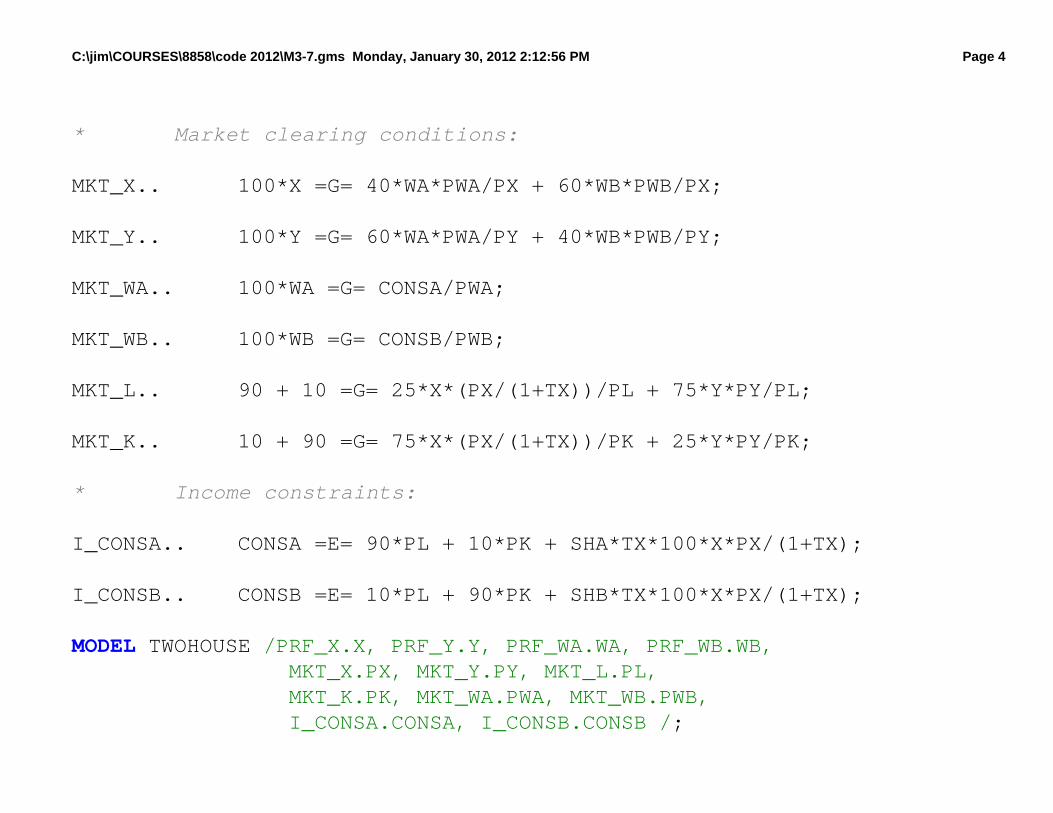
* Market clearing conditions:
MKT_X.. 100*X =G= 40*WA*PWA/PX + 60*WB*PWB/PX;
MKT_Y.. 100*Y =G= 60*WA*PWA/PY + 40*WB*PWB/PY;
MKT_WA.. 100*WA =G= CONSA/PWA;
MKT_WB.. 100*WB =G= CONSB/PWB;
MKT_L.. 90 + 10 =G= 25*X*(PX/(1+TX))/PL + 75*Y*PY/PL;
MKT_K.. 10 + 90 =G= 75*X*(PX/(1+TX))/PK + 25*Y*PY/PK;
* Income constraints:
I_CONSA.. CONSA =E= 90*PL + 10*PK + SHA*TX*100*X*PX/(1+TX);
I_CONSB.. CONSB =E= 10*PL + 90*PK + SHB*TX*100*X*PX/(1+TX);
MODEL TWOHOUSE /PRF_X.X, PRF_Y.Y, PRF_WA.WA, PRF_WB.WB, MKT_X.PX, MKT_Y.PY, MKT_L.PL, MKT_K.PK, MKT_WA.PWA, MKT_WB.PWB, I_CONSA.CONSA, I_CONSB.CONSB /;
C:\jim\COURSES\8858\code 2012\M3-7.gms Monday, January 30, 2012 2:12:56 PM Page 5
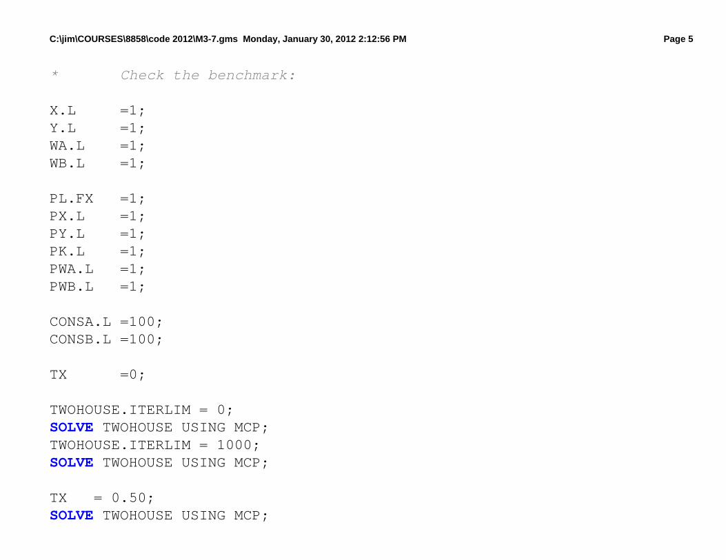
* Check the benchmark:
X.L =1;Y.L =1;WA.L =1;WB.L =1;
PL.FX =1;PX.L =1;PY.L =1;PK.L =1;PWA.L =1;PWB.L =1;
CONSA.L =100;CONSB.L =100;
TX =0;
TWOHOUSE.ITERLIM = 0;SOLVE TWOHOUSE USING MCP;TWOHOUSE.ITERLIM = 1000;SOLVE TWOHOUSE USING MCP;
TX = 0.50;SOLVE TWOHOUSE USING MCP;
C:\jim\COURSES\8858\code 2012\M3-7.gms Monday, January 30, 2012 2:12:56 PM Page 6
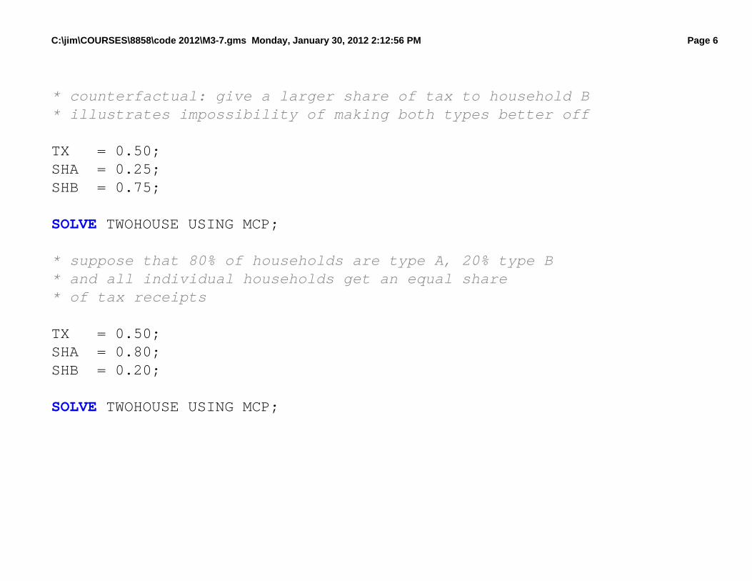
* counterfactual: give a larger share of tax to household B* illustrates impossibility of making both types better off
TX = 0.50;SHA = 0.25;SHB = 0.75;
SOLVE TWOHOUSE USING MCP;
* suppose that 80% of households are type A, 20% type B* and all individual households get an equal share* of tax receipts
TX = 0.50;SHA = 0.80;SHB = 0.20;
SOLVE TWOHOUSE USING MCP;
41
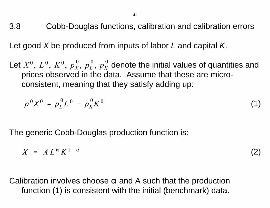
3.8 Cobb-Douglas functions, calibration and calibration errors
Let good X be produced from inputs of labor L and capital K.
Let denote the initial values of quantities andprices observed in the data. Assume that these are micro-consistent, meaning that they satisfy adding up:
(1)
The generic Cobb-Douglas production function is:
(2)
Calibration involves choose " and A such that the productionfunction (1) is consistent with the initial (benchmark) data.
42
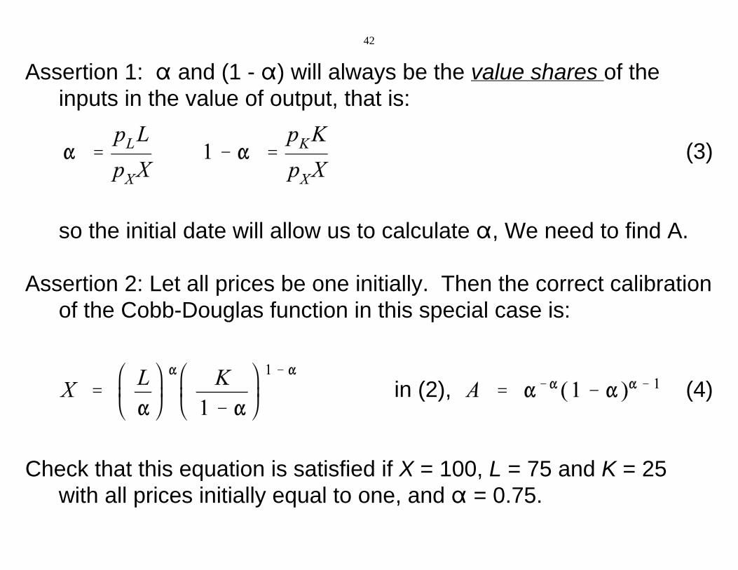
Assertion 1: " and (1 - ") will always be the value shares of theinputs in the value of output, that is:
(3)
so the initial date will allow us to calculate ", We need to find A.
Assertion 2: Let all prices be one initially. Then the correct calibrationof the Cobb-Douglas function in this special case is:
in (2), (4)
Check that this equation is satisfied if X = 100, L = 75 and K = 25with all prices initially equal to one, and " = 0.75.
43
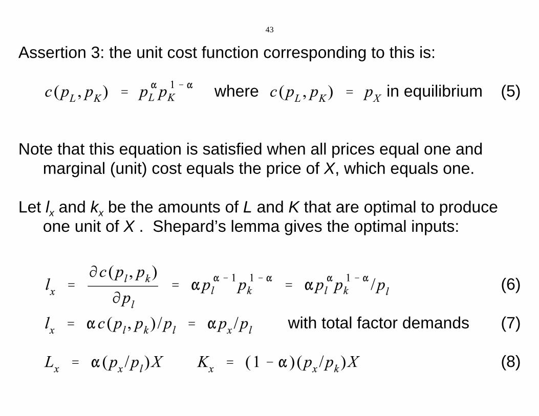
Assertion 3: the unit cost function corresponding to this is:
where in equilibrium (5)
Note that this equation is satisfied when all prices equal one andmarginal (unit) cost equals the price of X, which equals one.
Let lx and kx be the amounts of L and K that are optimal to produceone unit of X . Shepard’s lemma gives the optimal inputs:
(6)
with total factor demands (7)
(8)
44
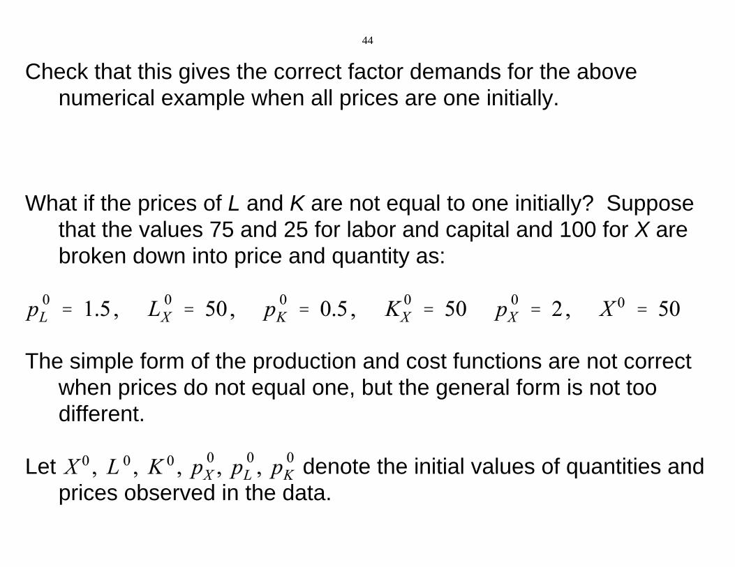
Check that this gives the correct factor demands for the abovenumerical example when all prices are one initially.
What if the prices of L and K are not equal to one initially? Supposethat the values 75 and 25 for labor and capital and 100 for X arebroken down into price and quantity as:
The simple form of the production and cost functions are not correctwhen prices do not equal one, but the general form is not toodifferent.
Let denote the initial values of quantities andprices observed in the data.
45
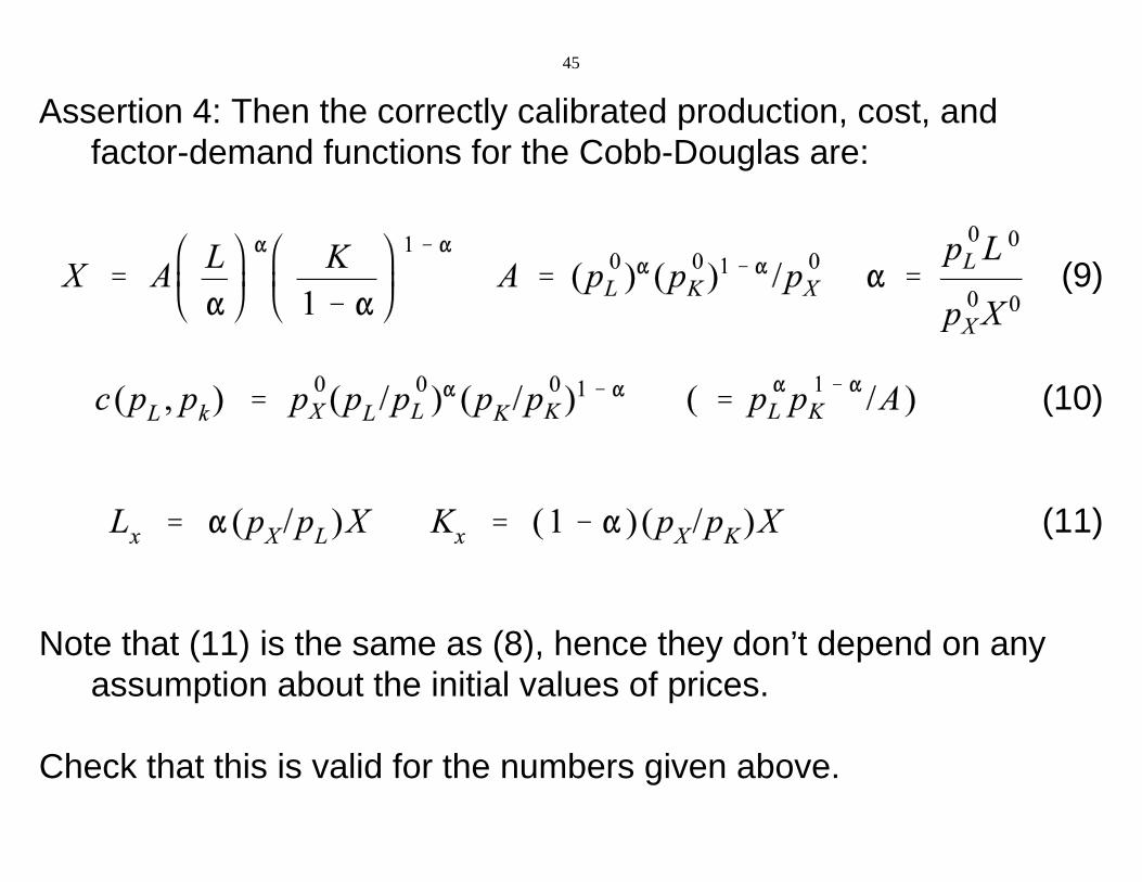
Assertion 4: Then the correctly calibrated production, cost, andfactor-demand functions for the Cobb-Douglas are:
(9)
(10)
(11)
Note that (11) is the same as (8), hence they don’t depend on anyassumption about the initial values of prices.
Check that this is valid for the numbers given above.
46
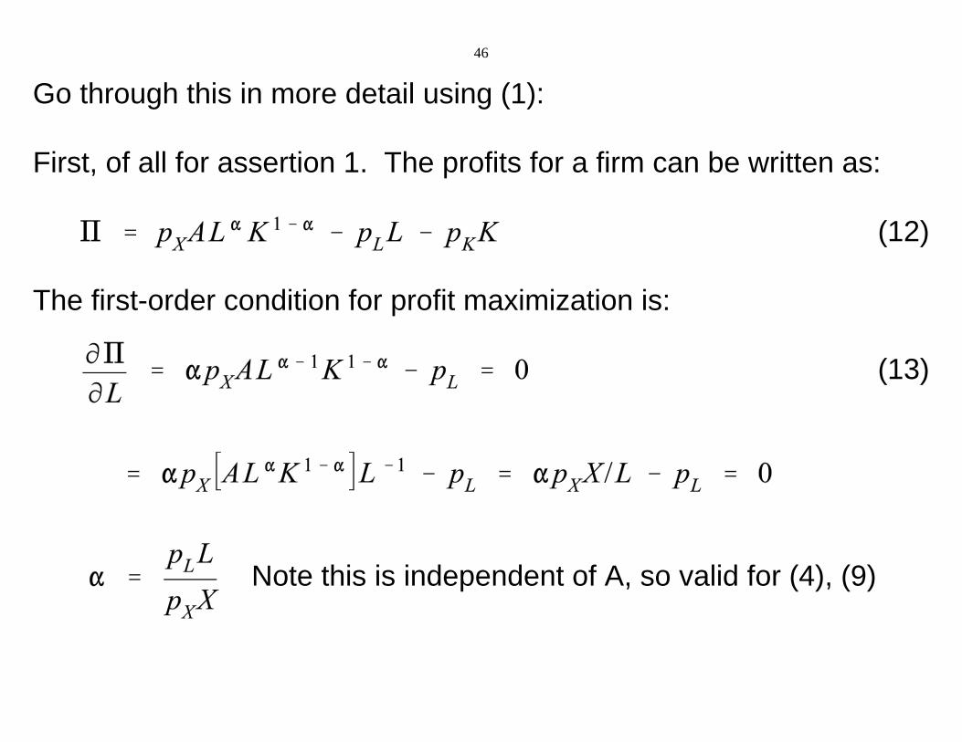
Go through this in more detail using (1):
First, of all for assertion 1. The profits for a firm can be written as:
(12)
The first-order condition for profit maximization is:
(13)
Note this is independent of A, so valid for (4), (9)

47
Assertion 5: For initial, micro-consistent values , the correct production function can be
written as:
where (14)
Check that this is satisfied for the initial values just mentioned.
Some multiplying and dividing will give us:
(15)
(16)
48
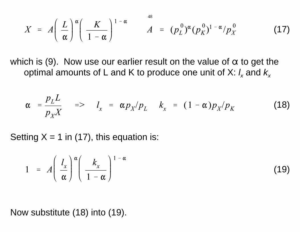
(17)
which is (9). Now use our earlier result on the value of " to get theoptimal amounts of L and K to produce one unit of X: lx and kx
(18)
Setting X = 1 in (17), this equation is:
(19)
Now substitute (18) into (19).
49
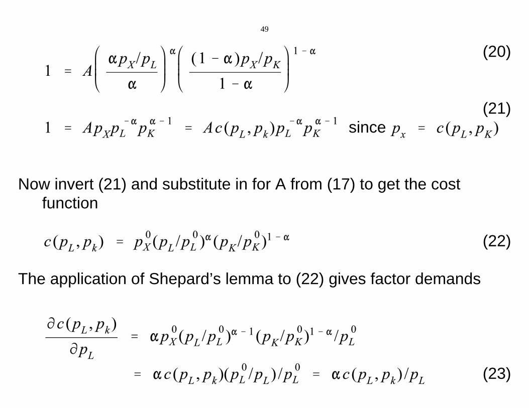
(20)
(21) since
Now invert (21) and substitute in for A from (17) to get the costfunction
(22)
The application of Shepard’s lemma to (22) gives factor demands
(23)
50
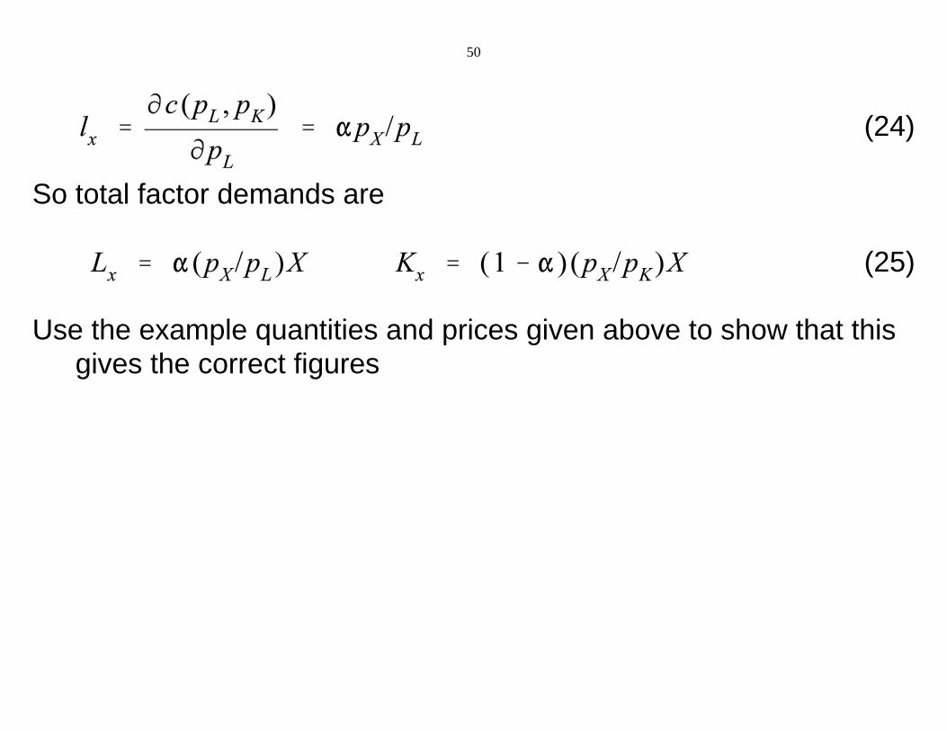
(24)
So total factor demands are
(25)
Use the example quantities and prices given above to show that thisgives the correct figures
51
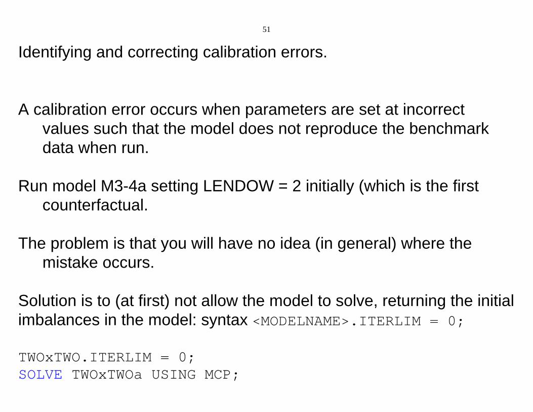
Identifying and correcting calibration errors.
A calibration error occurs when parameters are set at incorrectvalues such that the model does not reproduce the benchmarkdata when run.
Run model M3-4a setting LENDOW = 2 initially (which is the firstcounterfactual.
The problem is that you will have no idea (in general) where themistake occurs.
Solution is to (at first) not allow the model to solve, returning the initialimbalances in the model: syntax <MODELNAME>.ITERLIM = 0;
TWOxTWO.ITERLIM = 0;SOLVE TWOxTWOa USING MCP;
52
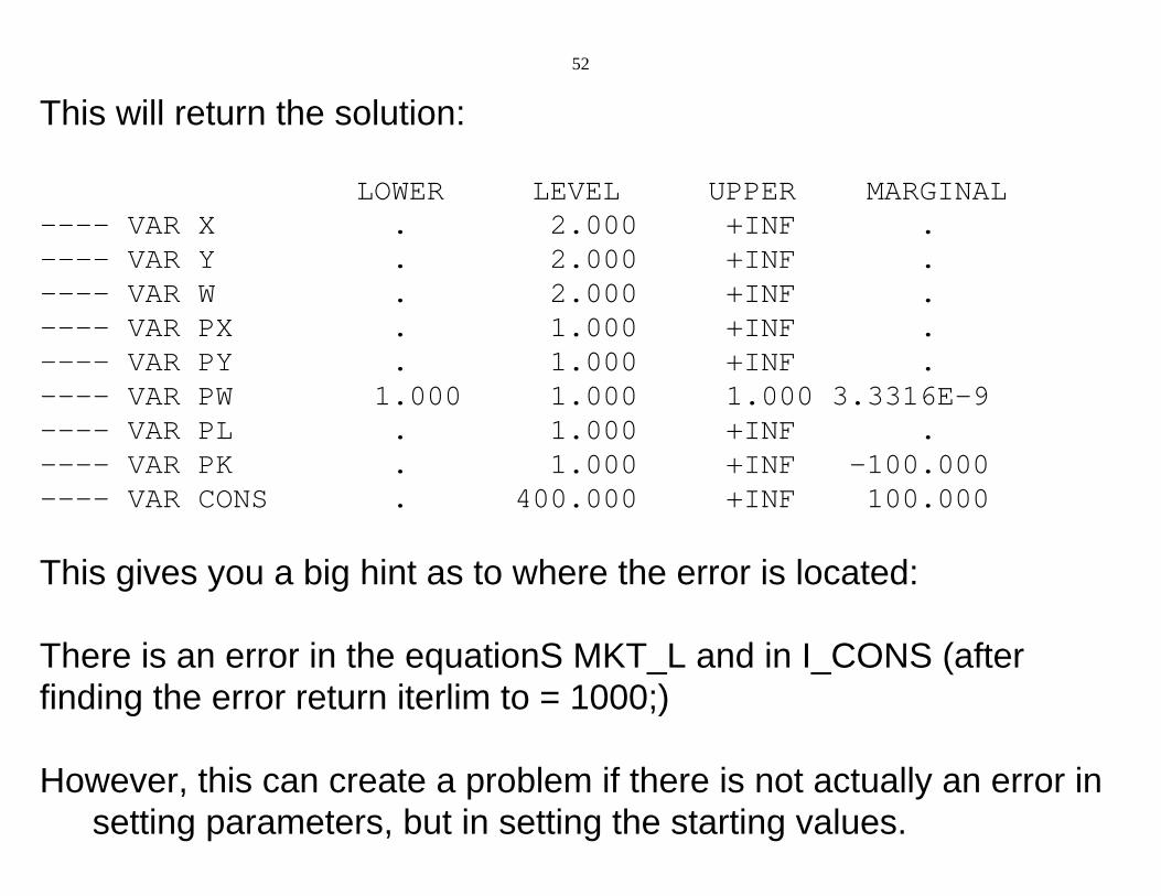
This will return the solution:
LOWER LEVEL UPPER MARGINAL---- VAR X . 2.000 +INF . ---- VAR Y . 2.000 +INF . ---- VAR W . 2.000 +INF . ---- VAR PX . 1.000 +INF . ---- VAR PY . 1.000 +INF . ---- VAR PW 1.000 1.000 1.000 3.3316E-9 ---- VAR PL . 1.000 +INF . ---- VAR PK . 1.000 +INF -100.000 ---- VAR CONS . 400.000 +INF 100.000
This gives you a big hint as to where the error is located:
There is an error in the equationS MKT_L and in I_CONS (afterfinding the error return iterlim to = 1000;)
However, this can create a problem if there is not actually an error insetting parameters, but in setting the starting values.
53
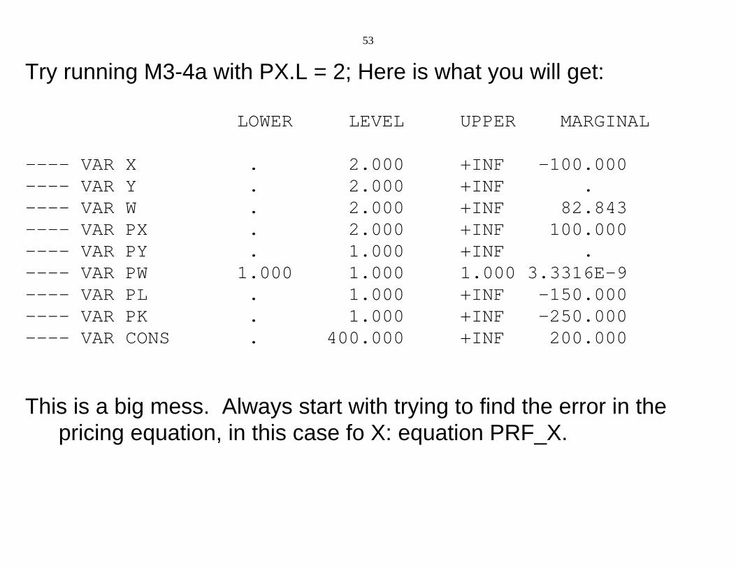
Try running M3-4a with PX.L = 2; Here is what you will get:
LOWER LEVEL UPPER MARGINAL
---- VAR X . 2.000 +INF -100.000 ---- VAR Y . 2.000 +INF . ---- VAR W . 2.000 +INF 82.843 ---- VAR PX . 2.000 +INF 100.000 ---- VAR PY . 1.000 +INF . ---- VAR PW 1.000 1.000 1.000 3.3316E-9 ---- VAR PL . 1.000 +INF -150.000 ---- VAR PK . 1.000 +INF -250.000 ---- VAR CONS . 400.000 +INF 200.000
This is a big mess. Always start with trying to find the error in thepricing equation, in this case fo X: equation PRF_X.
54
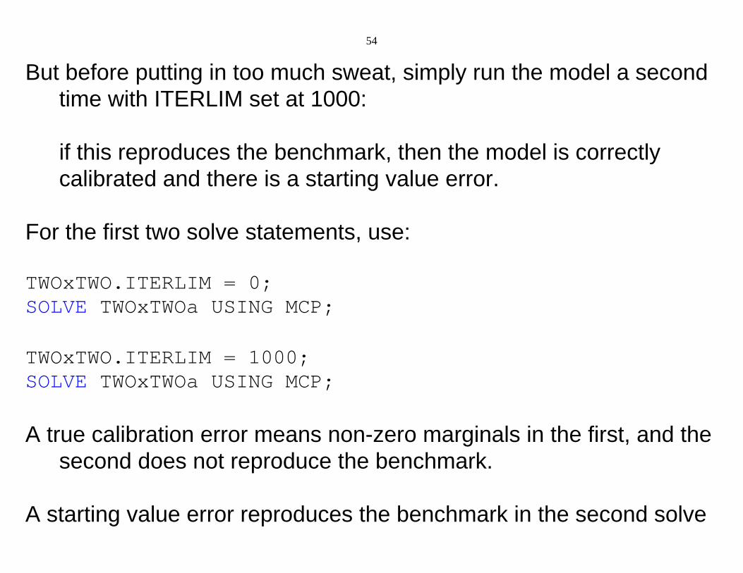
But before putting in too much sweat, simply run the model a secondtime with ITERLIM set at 1000:
if this reproduces the benchmark, then the model is correctlycalibrated and there is a starting value error.
For the first two solve statements, use:
TWOxTWO.ITERLIM = 0;SOLVE TWOxTWOa USING MCP;
TWOxTWO.ITERLIM = 1000;SOLVE TWOxTWOa USING MCP;
A true calibration error means non-zero marginals in the first, and thesecond does not reproduce the benchmark.
A starting value error reproduces the benchmark in the second solve